Extended-range percolation in complex networks

Abstract

Classical percolation theory underlies many processes of information transfer along the links of a network. In these standard situations, the requirement for two nodes to be able to communicate is the presence of at least one uninterrupted path of nodes between them. In a variety of more recent data transmission protocols, such as the communication of noisy data via error-correcting repeaters, both in classical and quantum networks, the requirement of an uninterrupted path is too strict: two nodes may be able to communicate even if all paths between them have interruptions/gaps consisting of nodes that may corrupt the message. In such a case a different approach is needed. We develop the theoretical framework for extended-range percolation in networks, describing the fundamental connectivity properties relevant to such models of information transfer. We obtain exact results, for any range $R$, for infinite random uncorrelated networks and we provide a message-passing formulation that works well in sparse real-world networks. The interplay of the extended range and heterogeneity leads to novel critical behavior in scale-free networks.

I Introduction

Percolation theory investigates how connectivity structures in a network change if some nodes or links are removed/deactivated Stauffer and Aharony (2018). Standard (classical) percolation uses a definition of connectedness whereby two active nodes belong to the same connected component if there is at least one uninterrupted path of active nodes between them newman2010networks; Li et al. (2021). This model setup provides the basis for the mathematical description of a wide range of physical processes, such as flow through porous media Moon and Girvin (1995), forest fires Henley (1993), epidemic spreading Moore and Newman (2000); Newman (2002); Pastor-Satorras et al. (2015) and various types of transport phenomena Barrat et al. (2008); Germano and de Moura (2006); Pei and Makse (2013); Zhang et al. (2016). A more recent, well-studied class of generalizations of standard percolation use connectivity definitions that involve multiple uninterrupted paths between nodes, such as in $k$-core Dorogovtsev et al. (2006) or bootstrap percolation Baxter et al. (2010) and in the mutual connectivity rule of multiplex networks Buldyrev et al. (2010). These models, particularly popular in recent years, are suitable for studying phenomena such as complex contagion Centola and Macy (2007) or multilayer spreading processes de Arruda et al. (2018).

In a variety of information spreading processes, however, connectivity definitions based solely on uninterrupted paths are not appropriate. In the case of noisy data transmission, for example, signals may deteriorate while passing through the nodes of a network, and the presence of well-positioned error-correcting repeaters is required for long-range communication. Quantum networks are particularly affected by such deterioration Coutinho et al. (2022). Similarly to the classical case, the communication range may be extended using well-placed quantum repeaters Zwerger et al. (2018); Pirandola (2019). For the purposes of quantum enhanced secure communication, one can circumvent the need for quantum repeaters using hybrid classical-quantum networks with trusted nodes Chen et al. (2021). In such networks there are some classical repeaters trusted to be secure, and one only needs to create a quantum connection from one of those repeaters to another. In processes of this kind, one may think of repeaters or trusted nodes as active, and long-distance communication may be possible even if there are no uninterrupted paths, provided active nodes along the paths are not too far apart. This calls for a theory of percolation that incorporates a connectivity definition allowing interruptions/gaps (sequences of inactive nodes) in the paths between nodes of the same connected component. We note that similar phenomena are also found in pure state quantum networks Perseguers et al. (2008, 2010); Meng et al. (2021) with non-trivial entanglement distribution that cannot be tackled using standard percolation.

Here we propose a general model of extended-range percolation on complex networks, aiming to provide a mathematical basis for information transmission involving path interruptions. Similar problems have been considered in the literature, although, to our knowledge, exclusively on lattices. In the context of magnetic systems, tunable interaction ranges were studied in the equivalent neighbour model of Domb, Dalton and Sykes Dalton et al. (1964); Domb and Dalton (1966). Numerous results exist on long-range percolation models where distant nodes of a lattice are connected with a decaying probability Schulman (1983); Aizenman and Newman (1986); Biskup and Lin (2019). More recent works include “extended neighbour percolation” Malarz (2015, 2020, 2021); Xun and Ziff (2020); Xun et al. (2021); Zhao et al. (2022); Xun et al. (2022) and the related “range-R” model in mathematics Frei and Perkins (2016); Hong (2023).

Surprisingly, extended-range percolation has not received any attention within the field of complex networks, thus an understanding of such problems on architectures that may realistically represent many modern information networks is lacking.

II Extended-range percolation model

In an arbitrary network, let each node be active independently with probability $\phi$, be inactive otherwise. Each active node $i$ is able to transmit information directly up to a topological distance $R$, that is, to all active nodes at most $R$ steps away from node $i$ in the network. By direct transmission we mean transmission without the help of any other active nodes potentially acting as repeaters. We define the extended-range connected component of node $i$ as the set of active nodes that node $i$ is able to transmit information to or receive information from, either directly or indirectly, via relays of intermediate active nodes. (Note that $R=1$ corresponds to standard nearest neighbour percolation.) Fig. 1(a) shows an example of a small network with two extended-range connected components, where active nodes have a range $R=2$. A perhaps more instructive definition may be given as follows. Two nodes belong to the same extended-range connected component if there is at least one walk between them in which there are at most $R-1$ consecutive inactive nodes. Note that we must use ”walks” instead of ”paths” in the definition. This is because two nodes may be indirectly connected via a third intermediate node which is not on the path between them. As an example, see Fig. 1(f) where two active black nodes are shown on a chain, at a distance of four steps from each other, therefore not being directly connected for range parameter $R=3$. An additional off-path active (bridge) node, however, marked in green, is able to indirectly connect the two nodes, so that they belong to the same extended-range connected component. In contrast [Fig. 1(d),(e)] off-path bridges do not allow indirect connections for $R<3$. This feature introduces a complex combinatorial problem for high values of $R$, as we detail below. Here we derive the exact solution of extended-range percolation on infinite random uncorrelated networks of arbitrary degree distribution. We start with $R=2$, where off-path bridges do not play any role, we then tackle the additional complexity due to off-path bridges for $R=3$ and $4$, then we further generalize to any $R$. We also present an efficient message-passing formulation of the theory that works well in finite real-world networks.

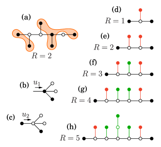
Figure 1: Panel (a): A small network with two distinct extended-range connected components, shaded orange. Active nodes (filled black circles) have a range of $R=2$. Inactive nodes are represented by empty circles. Panels (b) and (c) are schematic representations of Eqs. (1) and (2), respectively. Panels (d)-(h) illustrate the concept of off-path bridge nodes and the increasing complexity of the problem for larger values of the range $R$. Empty nodes are inactive, filled nodes are active. The two active black nodes are not directly connected, being at distance $R+1$. The red nodes, even if active, do not connect the black nodes indirectly. However, for $R>2$, any of the green nodes, which are not on the path connecting the two black nodes, play the role of a bridge, indirectly connecting them.

III Exact solution in uncorrelated networks

Let us consider a random uncorrelated network with an arbitrary degree distribution $p_{k}$, in the infinite size limit. We start by solving the problem of finding the size of the extended-range giant connected component (EGCC) for $R=2$. Let $u_{1}$ be the probability that, following a random link with an active end node, we are not able to reach the EGCC via walks that have gaps of at most one consecutive inactive node. Probability $u_{1}$ is suggestively written as $u_{1}=P_{\rightarrow\newmoon}$. Note that the starting node’s state does not play any role. Let $u_{2}$ be the probability that following a random link with an inactive end node and active starting node, we are not able to reach the EGCC via allowed walks: $u_{2}=P_{\newmoon\rightarrow\fullmoon}$. A simple equation for $u_{1}$ is written by noting that [see Fig. 1(b)] after reaching an active node, the branch is finite only if all $r$ outgoing neighbors are either active but do not lead to the EGCC (prob. $\phi u_{1}$) or inactive and not leading to the EGCC (prob. $(1-\phi)u_{2}$). Exploiting the local treelikeness of the networks, we can write

$$u_{1}=\sum_{r=0}^{\infty}q_{r}\big{(}\phi u_{1}+(1-\phi)u_{2}\big{)}^{r}=g_{1}\big{(}\phi u_{1}+(1-\phi)u_{2}\big{)},$$ (1)

where $q_{r}$ is the excess degree distribution and $g_{1}$ is its probability generating function. The equation for the probability $u_{2}$ is similar, but in this case, having arrived from an active node to an inactive one, any inactive outgoing neighbor surely does not lead to the EGCC (see Fig. 1(c)),

$$u_{2}=g_{1}\big{(}\phi u_{1}+(1-\phi)\big{)}.$$ (2)

The relative size of the EGCC (probability of a randomly chosen node belonging to the EGCC) is

$$S=\phi\Big{[}1-g_{0}\Big{(}\phi u_{1}+(1-\phi)u_{2}\Big{)}\Big{]},$$ (3)

where $g_{0}$ is the generating function for the degree distribution $p_{k}$. Setting $u_{2}=1$ leads back to standard nearest-neighbor percolation.

Extending the theory to $R=3$ and $R=4$ requires the introduction of two other probabilities. Let us define $u_{3}$ as the probability that, following a random link with an inactive end node, and an inactive starting node, but with at least one active neighbor of the starting node, we are not able to reach the EGCC via allowed walks: $u_{3}=P_{\newmoon\relbar\fullmoon\rightarrow\fullmoon}$. Finally, $u_{4}$ is the probability that we are not able to reach the EGCC via allowed walks, by following a link that has an inactive end node, and has at least one active node at a distance 3 in the “reverse direction”, but no active nodes at shorter distances: $u_{4}=P_{\newmoon\relbar\fullmoon\relbar\fullmoon\rightarrow\fullmoon}$. In the case $2<R\leq 4$ the equation for $u_{1}$ remains the same, while the equation for $u_{2}$ is trivially modified, as one has to take into account that the EGCC could be reached, with probability $u_{3}$, even if the neighbor of an inactive node is inactive [see Fig. 1(c)],

$$u_{2}=g_{1}\big{(}\phi u_{1}+(1-\phi)u_{3}\big{)}.$$ (4)

The equation for $u_{3}$ is more complicated because it may happen [see Fig. 1(f) for the case of $R=3$] that two nodes belong to the same component even if there are three inactive nodes along the path between them. The indirect connection is guaranteed by the presence of an active off-path bridge node [the green node in Fig. 1(f)] which is at a distance $3$ from both of them. [The same phenomenon is shown in Fig. 1(g) for $R=4$.] Taking explicitly into account this possibility, for $R=4$ the equations for $u_{3}$ and $u_{4}$ are (see Appendix A for details)

$$u_{3} =g_{1}\big{(}(1-\phi)u_{4}\big{)}+g_{1}\big{(}\phi u_{1}+(1-\phi)u_{3}\big{)}-g_{1}\big{(}(1-\phi)u_{3}\big{)},$$ (5)

$$u_{4} =g_{1}(1-\phi)+g_{1}\big{(}\phi u_{1}+(1-\phi)u_{3}\big{)}-g_{1}\big{(}(1-\phi)u_{3}\big{)}.$$ (6)

For $R=3$, Eq. (6) is simply replaced by $u_{4}=1$.

The extension of the approach to $R>4$ is highly nontrivial, as it requires the introduction of increasingly complex conditional probabilities. Physically, this is due to the fact that bridges involve off-path nodes at increasing distances from the path [Fig. 1(h)]. See the Appendix for a presentation of the framework valid for any $R$ and the explicit equations for $R=5$ and $R=6$.

Our approach is exact for random uncorrelated locally tree-like networks with an arbitrary degree distribution. To find the solution, up to arbitrary precision, the equations for the probabilities $u_{i}$ may be iterated until convergence. Together with Eq. (3) they allow to determine the size of the EGCC. Fig. 2(a) displays the behavior of $S$ calculated using the numerical solutions of the equations for the probabilities $u_{i}$, for an Erdős-Rényi network of mean degree $\langle k\rangle=1.5$, for $R=1,\ldots,4$. Simulation results are also shown and demonstrate perfect agreement with the theoretical predictions. Equally perfect agreement is shown in the Appendix for power-law distributed networks. As expected, the size of the EGCC is zero up to a percolation threshold $\phi_{c}^{(R)}$, which gets smaller as $R$ is increased.

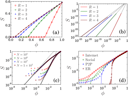
Figure 2: Relative size $S$ of the EGCC as a function of node activation probability $\phi$. (a) Predictions obtained solving numerically the equations for the $u_{i}$ (solid lines) compared with simulation results (symbols) for an Erdős-Rényi network of $\langle k\rangle=1.5$, for $R=1,\ldots,4$. (b) Numerical solutions of the same equations (solid lines) compared with the predicted singular behavior (dashed black lines) for power-law networks [Eqs. (III)] with $\gamma=2.5$ for $R=1,\ldots,4$. (c) Comparison of the numerical solutions of Eqs. (1), (2) and (3) (solid black lines) with simulation results for $\gamma=2.5$, $R=1$ (squares) and $R=2$ (triangles), for different network sizes. The dashed black lines correspond to the predicted singular behaviour [see Eqs. (III) for $R=2$ and Ref. Radicchi and Castellano (2015) for the standard $R=1$ case]. Analogous results for $\gamma>3$ are shown in Appendix D. (d) Solutions of the message-passing equations (10), (11) and (12) (solid lines) compared with simulation results (symbols) for three example real-world networks and an Erdős-Rényi network of $\langle k\rangle=4$.

To determine the critical threshold, let us consider for simplicity the case $R=4$. Eqs. (1), (4), (5) and (6) have the trivial solution $u_{1}=u_{2}=u_{3}=u_{4}=1$ for any value of $\phi$, which corresponds to $S=0$. This solution becomes unstable at the critical threshold $\phi_{c}^{(R=4)}$, above which the only stable solution corresponds to $S>0$. To find this threshold, we study the stability of the trivial solution by linearizing the equations around it, to obtain the Jacobian matrix

$$\hat{J}=b\begin{pmatrix}\phi&1-\phi&0&0\\ \phi&0&1-\phi&0\\ \phi&0&\frac{(1-\phi)[b-g_{1}^{\prime}(1-\phi)]}{b}&\frac{(1-\phi)g_{1}^{\prime}(1-\phi)}{b}\\ \phi&0&\frac{(1-\phi)[b-g_{1}^{\prime}(1-\phi)]}{b}&0\end{pmatrix},$$ (7)

where $b$ is the mean branching, $b=\langle k(k-1)\rangle/\langle k\rangle$. Using the Perron-Frobenius theorem, the critical threshold occurs when $\lambda_{1}$, the largest real eigenvalue of $\hat{J}$ is equal to $1$. Thus the critical condition is $\det[\hat{J}-\hat{I}]=0$, where $\hat{I}$ is the identity matrix. For $R<4$ the same methodology applies, only we must consider the appropriate smaller matrix of dimensions $R\times R$ in the top left corner of matrix $\hat{J}$. In this way we recover the standard percolation threshold ($R=1$) and a simple formula for the threshold in the case of $R=2$,

$$\phi_{c}^{(R=1)}=\frac{1}{b},\quad\quad\phi_{c}^{(R=2)}=\frac{1+b-\sqrt{(1+b)^{2}-4}}{2b}.$$ (8)

Analyzing the asymptotics of $\phi_{c}^{(R=2)}$ we obtain that $\phi_{c}^{(R=2)}\to b^{-2}$ for $b\to\infty$. For $R=3$ and $R=4$ the critical condition does not reduce to an algebraic equation for $\phi_{c}^{(R)}$, but may be solved easily by numerical means.

By expanding the r.h.s. of Eqs. (1), (4), (5), (6) and (3) in powers of $\epsilon_{i}=1-u_{i}$ one can show (see Appendix D) that, close to the threshold, the size of the EGCC behaves as $S\sim(\phi-\phi_{c}^{(R)})^{\beta}$, with $\beta=1$ for non-heterogeneous networks, i.e. networks whose degree distributions have a finite third moment, which includes ER networks and power-law degree-distributed networks, $p_{k}\sim k^{-\gamma}$, with $\gamma>4$. For weakly heterogeneous networks, with $3<\gamma<4$, we find the nontrivial exponent $\beta=1/(\gamma-3)$ as in ordinary percolation Radicchi and Castellano (2015). For strongly heterogeneous networks, with $2<\gamma<3$, we find a non-universal behavior, with a critical exponent depending both on $\gamma$ and $R$. In particular, $S\sim\phi^{\beta}$, with

$$\beta= 1+\frac{\gamma-2}{1-(\gamma-2)^{2}} ~{}~{}~{}~{}\textrm{for }R=2,$$

$$\beta= 1+(\gamma-2)^{R-1} ~{}~{}~{}~{}\textrm{for }R>2.$$ (9)

Panels (b) and (c) of Fig. (2) display the $R$-dependence of the critical behavior of $S$ and show, for $R=2$, that numerical simulations agree with the predicted behavior. The dependence on $R$ may be surprising at first glance, since the present extended-range percolation model is not “long-range” (interaction ranges are finite) as opposed to truly long-range percolation Cirigliano et al. (2022). The nonuniversality stems from the fact that for strongly heterogeneous networks ($\gamma<3$), the average number of second (and third, fourth, etc.) neighbors is infinite, hence each node is able to interact with an infinite number of peers.

IV Message-passing equations

Based on Eqs. (1), (4), (5), (6) and (3), it is straightforward to construct a set of message-passing equations for the case of $R\leq 4$, to allow for an approximate solution of extended-range percolation on non-random networks, specified by a given adjacency matrix. Here we present the special case of $R\leq 2$, the general description may be found in Appendix E. For $R=2$ the message-passing equations corresponding to the self-consistency equations (1) and (2) are written as

$$u^{(i\leftarrow j)}_{1} =\prod_{k\in\partial_{j}\setminus i}\left[\phi u^{(j\leftarrow k)}_{1}+(1-\phi)u^{(j\leftarrow k)}_{2}\right],$$ (10)

$$u^{(i\leftarrow j)}_{2} =\prod_{k\in\partial_{j}\setminus i}\left[\phi u^{(j\leftarrow k)}_{1}+1-\phi\right],$$ (11)

where $\partial_{j}$ denotes the set of neighbors of node $j$. The quantity $u^{(i\leftarrow j)}_{1}$ is the probability that following link $(ij)$, in the direction of $j$, we are not able to reach the EGCC via walks that have gaps of at most one inactive node, given that node $j$ is active. Similarly, $u^{(i\leftarrow j)}_{2}$ is the probability that following link $(ij)$, in the direction of $j$, we are not able to reach the EGCC via walks that have gaps of at most one inactive node, given that node $j$ is inactive and node $i$ is active. Eqs. (10) and (11) are asymptotically exact (in the infinite size limit) in locally treelike networks. The probability that node $i$ belongs to the EGCC can then be expressed as

$$S_{i}=\phi\left[1-\prod_{j\in\partial_{i}}\left(\phi u^{(i\leftarrow j)}_{1}+(1-\phi)u^{(i\leftarrow j)}_{2}\right)\right],$$ (12)

and the relative size of the EGCC as the average $S=N^{-1}\sum_{i=1}^{N}S_{i}$, where $N$ is the number of nodes. Fig. 2(d) shows message-passing results compared with simulation results, for an Erdős-Rényi network and three example real-world networks (see Appendix F for details). The correspondence is perfect in the case of Erdős-Rényi, as expected, and also very good for the real-world networks containing short loops. In the case of the network “Social” the fit is somewhat poorer, due to the very high average clustering coefficient in this network, $C\approx 0.65$.

Within the message-passing approach the critical threshold $\phi_{c}^{(R)}$ may be obtained by following the standard procedure, i.e., linearizing Eqs. (10), (11) around the trivial solution, $u^{(i\leftarrow j)}_{1}=u^{(i\leftarrow j)}_{2}=1$ for all links $(ij)$. We obtain, for $R=2$, the Jacobian matrix

$$\hat{C}=\begin{pmatrix}\phi\hat{B}&(1-\phi)\hat{B}\\ \phi\hat{B}&0\end{pmatrix},$$ (13)

where $\hat{B}$ is the nonbacktracking (or Hashimoto) matrix Krzakala et al. (2013). The largest eigenvalue of matrix $\hat{C}$ must be $1$ at the threshold. The solution may be found numerically; e.g., Ref. Baxter and Timár (2021) provides an adaptation of the Newton-Raphson method for such problems, whereby one can quickly find $\phi_{c}^{(R=2)}$ to arbitrary precision. When $R=1$, we have $\hat{C}=\phi\hat{B}$, and the problem reduces to the message-passing formulation of ordinary percolation Karrer et al. (2014).

V Non-uniform range parameter

One may consider a more general version of the model presented above, where the range parameter of each node is allowed to be different. Specifically, let each active node $i$ be able to transmit information directly up to a topological distance $R_{i}$. We define the extended-range out-component $s_{\textrm{out}}(i)$ of node $i$ as the set of active nodes to which node $i$ is able to transmit information, either directly or indirectly, via relays of intermediate active nodes. Fig. 3(a) shows an example of a small network with the extended-range out-component of node $i$ shaded orange. Note that node $i$ is only able to directly transmit information to one active node, while two further active nodes are reached indirectly. The extended-range in-component $s_{\textrm{in}}(i)$ of node $i$ is the set of all active nodes that are able to transmit information to node $i$, either directly or indirectly [see Fig. 3(b), shaded blue]. In the case of uniform range parameter ($R_{i}=R$) the extended-range out- and in-components of any node coincide and are equivalent to the extended-range connected component, defined in Sec. II.

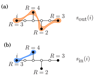
Figure 3: Extended-range out-component (a) and in-component (b) of node $i$. The range of each active node (filled black circles) is indicated near it.

It is interesting to note that the non-uniform extended-range percolation model on any network is equivalent to standard directed percolation on a modified network where we add directed links pointing from all nodes $i$ to all other nodes at most a distance $R_{i}$ from node $i$. (The original links should be considered undirected, or “bidirectional”.) As a result, the concept of strong connectivity, as well as a rich variety of topologically different components emerge, as in standard directed percolation Broder et al. (2000); Timár et al. (2017).

VI Discussion and conclusions

We have presented a framework for solving extended-range percolation exactly on locally tree-like networks. This generalization of ordinary percolation, allowing for gaps in the walks connecting distant nodes, provides a fundamental topological description of connectivity properties in noisy quantum networks, hybrid classical-quantum networks with trusted nodes, or classical data transmission networks using error-correcting repeaters. Our results, combined with existing methods of optimal percolation Morone and Makse (2015); Morone et al. (2016); Braunstein et al. (2016) may suggest possible strategies for the optimal placement of repeaters (or trusted nodes) in such communication networks.

Other interesting perspectives are opened by our work. The approach presented here may be used and extended to further analyze the critical properties of the extended-range percolation transition in networks, beyond the derivation of the exponent $\beta$, including in particular finite-size scaling and the distribution of finite extended-range connected components Cirigliano et al. (a).

Extended-range percolation on a generic undirected graph $\mathcal{G}_{0}^{(u)}$ can actually be seen, if all $R_{i}=R$, as a standard nearest-neighbor percolation process on a different graph $\mathcal{G}_{1}^{(u)}$, obtained from the original one by adding a link from each node $i$ to all other nodes at most $R$ steps away from it. The graph $\mathcal{G}_{1}^{(u)}$ is clearly highly clustered. Hence our approach, which exactly solves extended-range percolation on the original tree-like graph, provides also the exact solution for ordinary percolation on the corresponding graph with many intertwined short loops. This is a rare case of a highly clustered network model whose nontrivial percolation properties are exactly known. The formation of the $\mathcal{G}_{1}^{(u)}$ clustered graph by the addition of links among neighbors at short distances, can be seen as a variant of the triadic closure mechanism, prevalent in many real-world networks Asikainen et al. (2020). Our results may therefore also aid the development of more precise theories of percolation and related processes (e.g., epidemic spreading) in such cases. Exploring the topological properties of $\mathcal{G}_{1}^{(u)}$ Cirigliano et al. (b) and of the directed graphs $\mathcal{G}_{1}^{(d)}$ arising in the case of non-uniform range parameters $R_{i}$, presents an additional interesting avenue for future research.

Another intriguing aspect of extended-range percolation is the question of how site and bond percolation are related in this problem. We have considered site percolation in this work, for which it is true that extended-range percolation on a graph $\mathcal{G}_{0}^{(u)}$ is equivalent to standard percolation on the modified graph $\mathcal{G}_{1}^{(u)}$, defined above. The same does not hold for bond percolation, however. It would be interesting to compare the critical thresholds and critical exponents of the two types of processes, and to find an interpretation of extended-range bond percolation in terms of the modified graph $\mathcal{G}_{1}^{(u)}$.

Appendix A Derivation of the equations in the case $R=4$

In this section we present the derivation of Eqs. $(5)$ and $(6)$ in the main text. We refer to the main text for the definition of the probabilities $u_{1}=P_{\rightarrow\newmoon}$, $u_{2}=P_{\newmoon\rightarrow\fullmoon}$, $u_{3}=P_{\newmoon\relbar\fullmoon\rightarrow\fullmoon}$ and $u_{4}=P_{\newmoon\relbar\fullmoon\relbar\fullmoon\rightarrow\fullmoon}$ and for the derivation of the equations for $u_{1}$ and $u_{2}$. Concerning $u_{3}$, let us look at Fig.4 and consider node $i$, the node at which we arrive following the configuration that corresponds to $u_{3}$. Let the number of outgoing neighbors, i.e., the excess degree at node $i$, be denoted by $r$. If none of the outgoing neighbors of node $i$ are active [Fig. 4(a)], an event occurring with probability $(1-\phi)^{r}$, the EGCC is not reached provided none of them leads to it, an event that occurs with probability $u_{4}$ for each of the independent branches. If instead there are $n>0$ active nodes among the $r$ outgoing neighbors [Fig. 4(b)], the probability of not reaching the EGCC is $(\phi u_{1})^{n}[(1-\phi)u_{3}]^{r-n}$. Note that in this case the branches are no longer independent, as the probability (of not reaching the EGCC) on a branch leading to an inactive node is modified by the presence of an active node in another branch, potentially acting as an off-path bridge node. Since only the number of active neighbors matters, and not where they are placed, ${r\choose n}$ configurations give the same contribution to $u_{3}$. Summing over $n$ we obtain

$$[(1-\phi)u_{4}]^{r}+\sum_{n=1}^{r}{r\choose n}(\phi u_{1})^{n}[(1-\phi)u_{3}]^{r-n}$$

$$=[(1-\phi)u_{4}]^{r}-[(1-\phi)u_{3}]^{r}+\sum_{n=0}^{r}{r\choose n}(\phi u_{1})^{n}[(1-\phi)u_{3}]^{r-n}$$

$$=[(1-\phi)u_{4}]^{r}-[(1-\phi)u_{3}]^{r}+\big{(}\phi u_{1}+(1-\phi)u_{3}\big{)}^{r}.$$

Finally, averaging over the excess degree distribution $q_{r}$ we get

$$u_{3} =\sum_{r}q_{r}\left\{[(1-\phi)u_{4}]^{r}-[(1-\phi)u_{3}]^{r}+\big{(}\phi u_{1}+(1-\phi)u_{3}\big{)}^{r}\right\}$$

$$=g_{1}\big{(}(1-\phi)u_{4}\big{)}-g_{1}\big{(}(1-\phi)u_{3}\big{)}+g_{1}(\phi u_{1}+(1-\phi)u_{3}),$$ (14)

which is Eq. (5) in the main text.

To derive $u_{4}$, the argument is perfectly analogous. If we arrive at node $i$ from a configuration ${\newmoon\relbar\fullmoon\relbar\fullmoon\rightarrow\fullmoon}$, then if none of the outgoing neighbors of node $i$ are active [Fig. 4(c)] the EGCC is not reached. This occurs with probability $(1-\phi)^{r}$. On the contrary, if at least one of the outgoing neighbors is active [Fig. 4(d)] then the probability of not reaching the EGCC on branches leading to inactive nodes is modified. Following the same procedure as above we get

$$u_{4}=g_{1}(1-\phi)-g_{1}\big{(}(1-\phi)u_{3}\big{)}+g_{1}(\phi u_{1}+(1-\phi)u_{3}),$$ (15)

which is Eq. $(6)$ in the main text.

These equations are valid for $R=4$. The equations for $R=3$ are obtained by simply setting $u_{4}=1$.

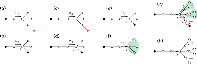
Figure 4: Visual representation of the recursive equations for $u_{3}$, $u_{4}$ and $u_{5}$. Panels (a)-(d) are for the case $R=4$, while panels (e)-(h) are for $R=5$. In (a) and (b) we have the two possible scenarios contributing to $u_{3}$. It is important to note that even if a second neighbor of node $i$ is active [the red node in panel (a)], the probability along the other branches still remains $(1-\phi)u_{4}$. In (c) and (d) the configurations contributing to $u_{4}$ are shown. Panels (e) and (f) show how the equations for $u_{4}$ must be modified for $R=5$ to take into account correlations among branches. Correlations due to off-path bridge nodes at distance $2$ are contained in the probability $u_{5}$. Panels (g) and (h) show the two possible scenarios contributing to $u_{5}$. In particular, from panels (g) and (h) we see that the probability of not reaching the EGCC via the configuration associated with node $l$ is different depending on whether node A, which belongs to another branch, is active or inactive.

Appendix B The equations for $R=5$

In the case $R=5$ the combinatorial difficulty of the problem is strongly increased, because one has to take into account dependencies between different branches arising due to off-path bridge nodes that are at distance 2 from the focal node $i$. A first observation is that the equation for $u_{3}$ remains the same as in the $R=4$ case, Eq. (14). This happens because if none of the outgoing neighbors of node $i$ are active, then even if we can reach an active node at distance $2$ from $i$, this does not change the probability along the other branches, which remains $u_{4}$, as one node at distance $4$ [the leftmost in Fig. 4(a)] is surely active. Hence in this case we can conclude that the branches are independent and the corresponding probability is $[(1-\phi)u_{4}]^{r}$. A similar argument implies that also the equations for $u_{1}$ and $u_{2}$ are unchanged.

Let us consider now the configuration ${\newmoon\relbar\fullmoon\relbar\fullmoon\rightarrow\fullmoon}$ corresponding to $u_{4}$ and let us call again $i$ the node at which we arrive. We must now consider the state of neighbors up to distance $2$, and the presence of an active second-neighbor node along one branch changes the probability of not reaching the EGCC along the others. We can start by distinguishing two complementary scenarios:

1. $n>0$ nodes of $i$’s first neighbors are active [Fig. 4(e)], i.e., there is at least one off-path bridge node at distance 1. In such a case we can repeat the argument presented above to derive Eq. (14) and conclude that the probability of not reaching the EGCC is

   $$v^{(r)}=\big{(}\phi u_{1}+(1-\phi)u_{3}\big{)}^{r}-((1-\phi)u_{3})^{r};$$ (16)

2. none of $i$’s first neighbors are active [Fig.4(f)]. In this case we denote the probability of not reaching the EGCC by $u^{(r)}_{5}$.

Hence we can write, averaging over the excess degree $r$,

$$u_{4}=\sum_{r}q_{r}\left(u^{(r)}_{5}+v^{(r)}\right)=u_{5}+v=u_{5}-g_{1}\big{(}(1-\phi)u_{3}\big{)}+g_{1}(\phi u_{1}+(1-\phi)u_{3}).$$ (17)

We still need an equation for the probability $u_{5}$. We stress that the meaning of $u_{5}$ is conceptually different from the previous $u_{i}$ defined for $i\leq 4$. Due to the possibility of having off-path bridge nodes at distance 2, the branches emanating from the focal point $i$ are not independent and $u_{5}$ is a probability associated with the state of all neighbors of node $i$. In particular, this means that $u_{5}\neq P_{\newmoon\relbar\fullmoon\relbar\fullmoon\relbar\fullmoon\rightarrow\fullmoon}$. Instead $u_{5}$ is defined as the probability of not reaching the EGCC following a link which ends up in a configuration consisting of an inactive node with all the outgoing neighbors inactive, arriving from a branch of the type ${\newmoon\relbar\fullmoon\relbar\fullmoon\rightarrow\fullmoon}$, i.e. knowing that an active node is at distance $3$ in the reverse direction [see Fig. 4(f), where this configuration of only inactive outgoing neighbors is shaded green]. Thus $u_{5}$ is the probability that the configuration in Fig. 4(f) does not lead to the EGCC. If we arrive at the configuration associated with $u^{(r)}_{5}$—that is, with $r$ empty outgoing neighbors—, then we must consider the state of nodes at distance $2$ from $i$ to calculate the probability that the EGCC is not reached.

Again, two complementary scenarios must be considered:

1. $n>0$ of the branches lead to an active second neighbor of node $i$ [Fig.4(g)], i.e., there is at least one off-path bridge node at distance 2.

2. none of the branches lead to an active second neighbor [Fig.4(h)].

Let us analyze the case (a). Consider a first neighbor $k$ of node $i$, with excess degree $\rho_{k}$ and $\tau_{k}\geq 1$ of its outgoing neighbors active. The probability of not reaching the EGCC through it is

$$\sum_{\tau_{k}=1}^{\rho_{k}}{\rho_{k}\choose\tau_{k}}(\phi u_{1})^{\tau_{k}}((1-\phi)u_{3})^{\rho_{k}-\tau_{k}}=v^{(\rho_{k})}.$$ (18)

For a first neighbor $l$ of node $i$ with none of the other neighbors active, the probability of not reaching the EGCC through it is instead $u^{(\rho_{l})}_{5}$. Note that we can use $u^{(\rho_{l})}_{5}$ because node $l$ in Fig.4(g) is at distance $3$ from node $A$, which is active, and no other active nodes at smaller distances are present. Summing over all the possible ways of placing these branches we obtain

$$\sum_{n=1}^{r}{r\choose n}\prod_{k=1}^{n}v^{(\rho_{k})}\prod_{l=1}^{r-n}u^{(\rho_{l})}_{5}.$$

Averaging over the excess degrees of nodes $k$ and $l$ we get

$$\sum_{n=1}^{r}{r\choose n}\prod_{k=1}^{n}v\prod_{l=1}^{r-n}u_{5}=\sum_{n=1}^{r}{r\choose n}v^{n}u_{5}^{r-n}=-u_{5}^{r}+\left(u_{5}+v\right)^{r}.$$ (19)

In the case (b) all second-neighbors of node $i$ are inactive [Fig. 4(h)]. This happens with probability $(1-\phi)^{\sum_{j=1}^{r}\rho_{j}}$, so that averaging over the excess degrees ${\rho_{j}}$ we get a contribution $\big{(}g_{1}(1-\phi)\big{)}^{r}$. Summing this last contribution with the other in Eq. (19), and averaging over the excess degree $r$, considering the overall multiplicative factor of $(1-\phi)^{r}$, we obtain

$$u_{5} =\sum_{r}q_{r}(1-\phi)^{r}\left[\big{(}g_{1}(1-\phi)\big{)}^{r}-u_{5}^{r}+\left(u_{5}+v\right)^{r}\right]$$

$$=g_{1}\big{(}(1-\phi)g_{1}(1-\phi)\big{)}-g_{1}\big{(}(1-\phi)u_{5}\big{)}+g_{1}\big{(}(1-\phi)(u_{5}+v)\big{)}.$$ (20)

Hence we end up with the two equations for $u_{4}$ and $u_{5}$

$$u_{4} =u_{5}-g_{1}\big{(}(1-\phi)u_{3}\big{)}+g_{1}(\phi u_{1}+(1-\phi)u_{3}),$$ (21)

$$u_{5} =g_{1}\big{(}(1-\phi)g_{1}(1-\phi)\big{)}-g_{1}\big{(}(1-\phi)u_{5}\big{)}+g_{1}\big{(}(1-\phi)(u_{5}-g_{1}\big{(}(1-\phi)u_{3}\big{)}+g_{1}(\phi u_{1}+(1-\phi)u_{3}))\big{)}.$$ (22)

Eqs. (21) and (22), together with the equations for $u_{1}$, $u_{2}$ and $u_{3}$ constitute a set of five recursive equations involving the five probabilities, $u_{1},\dots,u_{5}$. Solving them iteratively one can evaluate $S$ using Eq. (3) in the main text.

Appendix C The case $R>5$

Following the same lines of argument as above, it is straightforward to derive the equations for $R=6$ (the equations for $u_{i}$ up to $i=4$ are unchanged)

$$u_{5} =g_{1}\big{(}(1-\phi)u_{6}\big{)}-g_{1}\big{(}(1-\phi)u_{5}\big{)}+g_{1}\big{(}(1-\phi)(u_{5}-g_{1}\big{(}(1-\phi)u_{3}\big{)}+g_{1}(\phi u_{1}+(1-\phi)u_{3}))\big{)},$$ (23)

$$u_{6} =g_{1}\big{(}(1-\phi)g_{1}(1-\phi)\big{)}-g_{1}\big{(}(1-\phi)u_{5}\big{)}+g_{1}\big{(}(1-\phi)(u_{5}-g_{1}\big{(}(1-\phi)u_{3}\big{)}+g_{1}(\phi u_{1}+(1-\phi)u_{3}))\big{)}.$$ (24)

Here the probability $u_{6}$ corresponds to a configuration analogous to $u_{5}$, only in this case we arrive from a configuration where the active node in the reverse direction is one step further away. In other words, $u_{6}$ is the probability of not reaching the EGCC having arrived from a configuration of type ${\newmoon\relbar\fullmoon\relbar\fullmoon\relbar\fullmoon\rightarrow\fullmoon}$, given that all outgoing neighbors (of the node at which we arrive) are inactive. Setting $u_{6}=g_{1}(1-\phi)$ we recover the equations for $R=5$.

A similar scheme may be used also for $R>6$. For any value of $R$ one can set up $R$ equations for $R$ distinct probabilities $u_{1},\ldots,u_{R}$. For increasing $R$, off-path bridge nodes may be situated at larger and larger distances, therefore one must introduce probabilities corresponding to increasingly complex configurations. The probabilities $u_{i}$ for $i>6$ are analogous to $u_{5}$ and $u_{6}$, but are conditioned on all outgoing first, second, third, etc. neighbors being inactive. This would result in increasingly complex equations involving multiply nested generating functions. Note that the complexity of the configurations associated with the probabilities $u_{i}$, and consequently, the complexity of the corresponding equations, increases in steps of two, due to the general observation that off-path bridge nodes at distance $r$ can only play a role for $R\geq 2r+1$.

The theoretical predictions for $R=5$ and $R=6$ are tested in Fig. 5(a) and Fig. 5(b), which display $S(\phi)$ given by Eq. (3) in the main text and using the numerical solution of the equations for the probabilities $u_{i}$, for $R=1,\dots,6$, for power-law degree-distributed networks ($p_{k}\sim k^{-\gamma}$) with (a) $\gamma=3.5$ and (b) $\gamma=4.5$, respectively. In both cases, results of numerical simulations are in agreement with the theoretical predictions.

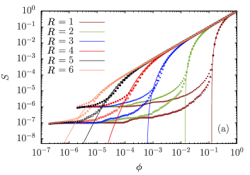
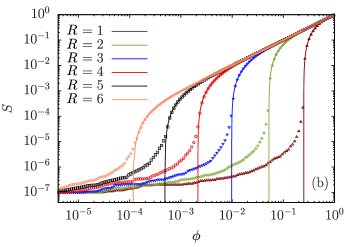
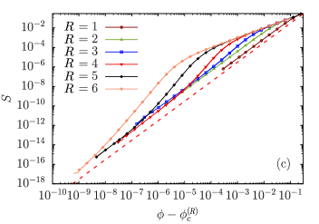
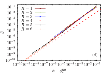
Figure 5: Top: comparison between numerical simulations (symbols), performed using a modification of the Newman-Ziff algorithm Newman and Ziff (2001), and exact solution (lines) obtained solving Eq. (3) in the paper and the recursive equations for the probabilities $u_{i}$ for $R=1,\dots,6$, for (a) $\gamma=3.5$, $N=10^{6}$ (full symbols), $N=10^{7}$ (empty symbols) and (b) $\gamma=4.5$, $N=10^{7}$, respectively. Bottom: scaling of the exact solution for $S$, obtained as before, versus $\delta\phi$, for (c) $\gamma=3.5$ and (d) $\gamma=4.5$, respectively. Dashed lines represent the scaling for $\delta\phi$ small with the exponent $\beta=1/(\gamma-3)$ and $\beta=1$ for figure (c) and (d) respectively, which are the exponents for the short-range ($R=1$) case.

Appendix D Critical properties

D.1 The critical threshold

For a generic extended-range percolation process with range $R$, the size of the EGCC is given by

$$S=\phi\left[1-g_{0}\left(\phi u_{1}+(1-\phi)u_{2}\right)\right],$$ (25)

where $u_{1}$ and $u_{2}$ are, in general, solutions of a nonlinear system of $R$ equations of the form

$$\boldsymbol{u}=\boldsymbol{F}(\boldsymbol{u};\phi),$$ (26)

with $\boldsymbol{u}$ an $R-$component vector $\boldsymbol{u}=(u_{1},u_{2},u_{3},u_{4},u_{5},u_{6},\dots)$ and $\boldsymbol{F}(\boldsymbol{u};\phi)=(F_{1}(\boldsymbol{u};\phi),F_{2}(\boldsymbol{u};\phi),\dots,F_{R}(\boldsymbol{u};\phi))$. Eq. (26) can be solved by iterating the recursive equation $\boldsymbol{u}(t+1)=\boldsymbol{F}(\boldsymbol{u}(t);\phi)$. Note that $\boldsymbol{u}^{\#}(\phi)=(1,1,1,1,g_{1}(1-\phi),g_{1}(1-\phi),\dots)$ is always a solution for any value of $R$ and for any $\phi$. This solution corresponds to $S=0$, the non-percolating phase. The solution $\boldsymbol{u}^{\#}$ is stable until $\phi$ reaches a critical value $\phi_{c}^{(R)}$: at this point, $\boldsymbol{u}^{\#}$ is marginally stable and another fixed point $\boldsymbol{u^{*}}$ appears, which is attractive for $\phi>\phi_{c}^{(R)}$. To analyze the stability of the trivial fixed point, we linearize the equations by setting $\boldsymbol{u}=\boldsymbol{u}^{\#}-\boldsymbol{\epsilon}$, from which it follows, using the fact that $\boldsymbol{u}^{\#}=\boldsymbol{F}(\boldsymbol{u}^{\#};\phi)$

$$\boldsymbol{\epsilon}(t+1)\simeq\hat{J}(\boldsymbol{u}^{\#};\phi)\boldsymbol{\epsilon}(t)$$ (27)

where $\hat{J}(\boldsymbol{u}^{\#};\phi)=D\boldsymbol{F}(\boldsymbol{u}^{\#};\phi)$ is the Jacobian matrix evaluated at the trivial fixed point. It follows that the trivial fixed point $\boldsymbol{u}^{\#}$, corresponding to $\boldsymbol{\epsilon}=0$, is an attractive solution if $\rho(\hat{J})<1$, where $\rho(\hat{J})$ is the spectral radius of $\hat{J}$. Furthermore, the Perron-Frobenius theorem Horn and Johnson (2012) tells us that the $\rho(\hat{J})=\lambda_{1}$, where $\lambda_{1}$ is the largest real eigenvalue of $\hat{J}$. Hence we can conclude that the critical threshold $\phi_{c}^{(R)}$ is the value such that

$$\det\left[\hat{J}(\boldsymbol{u}^{\#},\phi_{c}^{(R)})-\mathbb{1}\right]=0,$$ (28)

that is, when $\lambda_{1}$ equals $1$. At this point, $\boldsymbol{u}^{\#}$ becomes unstable and the other nontrivial fixed point $\boldsymbol{u^{*}}$, corresponding to a percolating phase with $S>0$, appears. Eq. (28) allows us to find the critical point for any $R$. Note that this argument holds if $g_{1}^{\prime}(1)$ exists, which means that the branching factor $b=\langle k(k-1)\rangle/\langle k\rangle$ must be finite. If instead the degree distribution has $b=\infty$, since for $R=1$ the threshold vanishes, we can conclude that $\phi_{c}^{(R)}=0$ for any $R$.

D.2 The exponent $\beta$

In this subsection we derive the value of the critical exponent $\beta$, determining the singularity of the EGCC size at the critical point

$$S\sim(\phi-\phi^{(R)}_{c})^{\beta}$$ (29)

The procedure is as follows:

1. we set $\phi=\phi^{(R)}_{c}+\delta\phi$, and consider small $\delta\phi$:

2. we expand the equations for $u_{i}$ around the trivial fixed point $u_{i}=u^{\#}_{i}-\epsilon_{i}$; it is sufficient to expand up to the two lowest orders in $\epsilon_{i}$;

3. we find the position of the nontrivial fixed point $\boldsymbol{\epsilon^{*}}\neq 0$ up to the lowest order in $\delta\phi$;

4. we expand $S$ above $\phi^{(R)}_{c}$ for small $\epsilon_{i}$ (since $\delta\phi$ is small) and we finally get an expression of the form $S\sim\delta\phi^{\beta}$.

Of particular interest is the case of power-law degree distributed networks with $p(k)\sim k^{-\gamma}\theta(k-k_{\text{min}})$, where $\theta(x)$ is the Heaviside step function, for which the procedure described above must be carried out carefully. The main tool is the asymptotic expansion for the generating functions close to their singular point $z=1$. The generating functions for power-law degree distribution $p(k)$ and excess degree distribution $q(r)=(r+1)p(r+1)/\langle k\rangle$, within the continuous-degree approximation, are

$$g_{0}(z) =\int_{0}^{\infty}dkp(k)z^{k}=(\gamma-1)k_{\text{min}}^{\gamma-1}\int_{k_{\text{min}}}^{\infty}dkk^{-\gamma}z^{k}=(\gamma-1)\frac{\Gamma(1-\gamma,k_{\text{min}}\psi)}{(k_{\text{min}}\psi)^{1-\gamma}},$$ (30)

$$g_{1}(z) =\int_{0}^{\infty}drq(r)z^{r}=(\gamma-2)k_{\text{min}}^{\gamma-2}\int_{k_{\text{min}}}^{\infty}dkk^{-(\gamma-1)}z^{k-1}=\frac{(\gamma-2)}{z}\frac{\Gamma(2-\gamma,k_{\text{min}}\psi)}{(k_{\text{min}}\psi)^{2-\gamma}},$$ (31)

where $\psi=\ln(1/z)$ and $\Gamma(a,x)$ is the Incomplete Gamma function. For $z\simeq 1$ the functions have a singular behavior which depends on the value of $\gamma$. The asymptotic expansion which keeps only the lowest order terms is presented in Appendix G.

D.3 The exponent $\beta$ for $R=2$

Setting $u_{1}=1-\epsilon_{1}$ and $u_{2}=1-\epsilon_{2}$, we have

$$S =\phi(1-g_{0}(\phi u_{1}+(1-\phi)u_{2})=\phi[1-g_{0}(1-(\phi\epsilon_{1}+(1-\phi)\epsilon_{2})],$$ (32)

where $\epsilon_{1}$ and $\epsilon_{2}$ are the solutions of the equations

$$1-\epsilon_{1} =g_{1}(\phi u_{1}+(1-\phi)u_{2})=g_{1}(1-(\phi\epsilon_{1}+(1-\phi)\epsilon_{2}),$$ (33)

$$1-\epsilon_{2} =g_{1}(\phi u_{1}+1-\phi)=g_{1}(1-\phi\epsilon_{1}).$$ (34)

Using Eq. (73) and Eq. (74) we get

$$S\simeq\left<k\right>\phi[\phi\epsilon_{1}+(1-\phi)\epsilon_{2}]$$ (35)

and

$$\epsilon_{1} \simeq B\phi\epsilon_{1}+B(1-\phi)\epsilon_{2}-\frac{D}{2}\left[\phi^{2}\epsilon_{1}^{2}+2\phi(1-\phi)\epsilon_{1}\epsilon_{2}+(1-\phi)^{2}\epsilon_{2}^{2}\right]-C(\gamma-2)(\phi\epsilon_{1}+(1-\phi)\epsilon_{2})^{\gamma-2},$$ (36)

$$\epsilon_{2} \simeq B\phi\epsilon_{1}-\frac{1}{2}D\phi^{2}\epsilon_{1}^{2}-C(\gamma-2)\phi^{\gamma-2}\epsilon_{1}^{\gamma-2}.$$ (37)

See Appendix G for the values of $\langle k\rangle$, $B$, $D$ and $C(\gamma-2)$. The solution of these equations for $\phi\simeq\phi_{c}^{(R=2)}$ depends on the value of $\gamma$.

D.3.1 Non-heterogeneous networks, i.e., $\gamma>4$ or ER networks

The leading terms in the equation for $\epsilon_{2}$ are those of order $\epsilon_{1}$ and $\epsilon_{1}^{2}$. Keeping only these two lowest order terms and inserting them into the equation for $\epsilon_{1}$, we get

$$\Lambda(\phi)\epsilon_{1}+\Omega\epsilon_{1}^{2}=0$$ (38)

where we set

$$\Lambda(\phi) =-(B\phi-1)-B^{2}\phi(1-\phi),$$ (39)

$$\Omega =\frac{D\phi^{2}}{2}\left[(B\large(1-\phi)+1\large)^{2}+B(1-\phi)\right].$$ (40)

which admits a nontrivial solution $\epsilon_{1}^{*}>0$

$$\epsilon_{1}^{*}=\left[\frac{-\Lambda(\phi)}{\Omega}\right]\simeq-\left[\frac{\Lambda(\phi_{c})+\Lambda^{\prime}(\phi_{c})\delta\phi}{\Omega}\right]=\left[-\frac{\Lambda^{\prime}(\phi_{c})\delta\phi}{\Omega}\right]\sim{\delta\phi}$$ (41)

as soon as $\phi>\phi_{c}$. We can conclude that both $\epsilon_{1}$ and $\epsilon_{2}$ are of $\mathcal{O}(\delta\phi)$, hence we get from Eq. (35) $\beta=1$. Notice that the same result holds for any uncorrelated random graph with finite $\langle k^{3}\rangle$, such as ER networks. This result is confirmed in Fig. 5(c).

D.3.2 Weakly-heterogeneous networks, i.e., $3<\gamma<4$

In this case the leading terms in the equation for $\epsilon_{2}$ are those of order $\epsilon_{1}$ and $\epsilon_{1}^{\gamma-2}$. Substituting $\epsilon_{2}$ in the equation for $\epsilon_{1}$ and keeping only lowest order terms gives

$$\Lambda(\phi)\epsilon_{1}+E\epsilon_{1}^{\gamma-2}=0,$$ (42)

where $\Lambda(\phi)$ is defined as before and

$$E=C(\gamma-2)\phi^{\gamma-2}\left[\large(1+B(1-\phi)\large)^{\gamma-2}+B(1-\phi)\right].$$ (43)

Hence the nontrivial solution $\epsilon_{1}^{*}$ is

$$\epsilon_{1}^{*}=\left[\frac{-\Lambda(\phi)}{E}\right]^{1/(\gamma-3)}\simeq\left[-\frac{\Lambda(\phi_{c})+\Lambda^{\prime}(\phi_{c})\delta\phi}{E}\right]^{1/(\gamma-3)}\sim(\delta\phi)^{1/(\gamma-3)}.$$ (44)

We conclude that both $\epsilon_{1}$ and $\epsilon_{2}$ are $\mathcal{O}((\delta\phi)^{1/(\gamma-3)})$. From Eq. (35) it follows that $\beta=1/(\gamma-3)$. This result is confirmed in Fig. 5(d).

D.3.3 Strongly-heterogenous networks: $2<\gamma<3$

In this case $\delta\phi=\phi$, since $\phi_{c}=0$. The leading terms in the equation for $\epsilon_{2}$ are again the ones considered in the case $3<\gamma<4$, but now the leading order is $(\phi\epsilon_{1})^{\gamma-2}$. This implies that, in the equation for $\epsilon_{1}$, the last term gives at leading order a contribution

$$\left[\phi\epsilon_{1}+(1-\phi)\epsilon_{2}\right]^{\gamma-2} \simeq\left[\phi\epsilon_{1}+(1-\phi)\large(B\phi\epsilon_{1}-C(\gamma-2)\phi^{\gamma-2}\epsilon_{1}^{\gamma-2}\large)\right]^{\gamma-2}$$

$$=\left[\phi\epsilon_{1}+B\phi(1-\phi)\epsilon_{1}-(1-\phi)C(\gamma-2)\phi^{\gamma-2}\epsilon_{1}^{\gamma-2}\right]^{\gamma-2}$$

$$=\left[-(1-\phi)C(\gamma-2)\phi^{\gamma-2}\epsilon_{1}^{\gamma-2}\right]^{\gamma-2}\left[1-\frac{1+B(1-\phi)}{(1-\phi)C(\gamma-2)\phi^{\gamma-2}}(\phi\epsilon_{1})^{3-\gamma}\right]^{\gamma-2}$$

$$\simeq\left[-(1-\phi)C(\gamma-2)\phi^{\gamma-2}\epsilon_{1}^{\gamma-2}\right]^{\gamma-2}\left[1-({\gamma-2})\frac{1+B(1-\phi)^{2}}{(1-\phi)C(\gamma-2)\phi^{\gamma-2}}(\phi\epsilon_{1})^{3-\gamma}+\dots\right]$$

$$\simeq\left[-(1-\phi)C(\gamma-2)\phi^{\gamma-2}\epsilon_{1}^{\gamma-2}\right]^{\gamma-2}$$

$$=\left[-(1-\phi)C(\gamma-2)\right]^{\gamma-2}\phi^{(\gamma-2)^{2}}\epsilon_{1}^{(\gamma-2)^{2}}.$$ (45)

Furthermore, since $\gamma-2<1$, the terms of order $\epsilon_{2}^{(\gamma-2)^{2}}$ dominate with respect to those of order $\epsilon_{1}^{\gamma-2}$ appearing in the equation for $\epsilon_{1}$. With this in mind, we get from the equation for $\epsilon_{1}$

$$\epsilon_{1}\simeq B\phi\epsilon_{1}+B^{2}\phi(1-\phi)\epsilon_{1}-B(1-\phi)C(\gamma-2)\phi^{\gamma-2}\epsilon_{1}^{\gamma-2}-C(\gamma-2)\left[-(1-\phi)C(\gamma-2)\phi^{\gamma-2}\epsilon_{1}^{\gamma-2}\right]^{\gamma-2}$$ (46)

which can be rewritten as

$$\epsilon_{1}\simeq\frac{B(1-\phi)C(\gamma-2)}{\Lambda(\phi)}\phi^{\gamma-2}\epsilon_{1}^{\gamma-2}+\left[\frac{-C(\gamma-2)\Large(-(1-\phi)C(\gamma-2)\Large)^{\gamma-2}}{\Lambda(\phi)}\right]\phi^{(\gamma-2)^{2}}\epsilon_{1}^{(\gamma-2)^{2}},$$ (47)

In the last expression, the exponent $(\gamma-2)^{2}$ is smaller than $\gamma-2$. Hence only the last term on the right hand side must be kept

$$\epsilon_{1}\simeq A\epsilon_{1}^{\alpha},$$ (48)

where we set

$$\alpha =(\gamma-2)^{2},$$ (49)

$$A =\left[\frac{-C(\gamma-2)\Large(-(1-\phi)C(\gamma-2)\Large)^{\gamma-2}}{\Lambda(\phi)}\right]\phi^{\alpha}.$$ (50)

As a consequence

$$\epsilon_{1}^{*}=A^{1/(1-\alpha)}\sim\phi^{(\gamma-2)^{2}/[1-(\gamma-2)^{2}]}.$$ (51)

From the equation for $\epsilon_{2}$ we get

$$\epsilon_{2}^{*}\sim\phi^{\gamma-2}\left(\phi^{(\gamma-2)^{2}/[1-(\gamma-2)^{2}]}\right)^{\gamma-2}\sim\phi^{(\gamma-2)/[1-(\gamma-2)^{2}]}.$$ (52)

From Eq. (35) we have

$$S \simeq\left<k\right>\phi^{2}\epsilon_{1}+\left<k\right>\phi\epsilon_{2}\sim\phi^{2+(\gamma-2)^{2}/[1-(\gamma-2)^{2}]}+\phi^{1+(\gamma-2)/[1-(\gamma-2)^{2}]}$$

$$\sim\phi^{1+(\gamma-2)/[1-(\gamma-2)^{2}]},$$ (53)

which implies

$$\beta_{(R=2)}=1+\frac{(\gamma-2)}{[1-(\gamma-2)^{2}]}.$$ (54)

Remarkably, while for $\gamma>3$ we recover the same exponent of standard percolation, for $2<\gamma<3$ we find a new nontrivial dependence of $\beta$ on $\gamma$, different from the one valid for $R=1$.

D.4 The exponent $\beta$ for $R>2$

For $\gamma>3$ the exponent $\beta$ is the same as for standard $R=1$ percolation even for $R>2$. This can be physically understood by considering that for $\gamma>3$ the extended-neighborhood always involves a large but finite number of nodes. Hence the $R$-range process cannot differ in the universal properties, i.e. in the critical exponents, from the $R=1$ case. From a mathematical point of view, one can easily check that all $\epsilon_{i}$ are of the same order, and hence the same scaling of $\epsilon_{1}$ versus $\delta\phi$ holds. As a consequence $S$ scales in the same way for any $R$ (see Fig. 5 (c) and (d)).

In the case $2<\gamma<3$, instead, the extended-neighborhood of a node reaches a diverging number of other nodes and this qualitatively changes the properties of the process.

Let us consider $R=6$. Noticing that $\phi u_{1}\ll u_{3}$ for $\phi\sim 0$, it is easy to see that the equation for $u_{6}=g_{1}(1-\phi)-\epsilon_{6}$, Eq. (24), yields, at lowest order

$$\epsilon_{6}\simeq g_{1}(1-\phi)-g_{1}\big{(}g_{1}(1-\phi)\big{)}\simeq-C(\gamma-2)\big{[}-C(\gamma-2)\phi^{\gamma-2}\big{]}^{\gamma-2}\sim\phi^{(\gamma-2)^{2}}.$$ (55)

From Eq. (23) for $u_{5}=g_{1}(1-\phi)-\epsilon_{5}$, we get

$$\epsilon_{5}\simeq g_{1}(1-\phi)-g_{1}\big{(}(1-\phi)u_{6}\big{)}\sim\phi^{(\gamma-2)^{3}}.$$ (56)

Considering Eq. (21) for $u_{4}=1-\epsilon_{4}$ it is also easy to realize that the leading contribution is provided by the first term on the r.h.s., $u_{5}$, which, expanded for small $\phi$ gives

$$\epsilon_{4}\sim\epsilon_{5}\sim\phi^{(\gamma-2)^{3}}.$$ (57)

In Eq. (14) for $u_{3}$ the leading contribution on the r.h.s. in the limit of small $\phi$, is the first, thus giving

$$\epsilon_{3}\sim\epsilon_{4}^{\gamma-2}\sim\phi^{(\gamma-2)^{4}}.$$ (58)

By the same token, inspection of the equations for $u_{2}$ and $u_{1}$ promptly leads to the conclusion that $\epsilon_{1}\sim\epsilon_{2}^{\gamma-2}\sim\epsilon_{3}^{(\gamma-2)^{2}}$.

From Eq. (35) we get

$$S\sim\phi\epsilon_{2}\sim\phi^{1+(\gamma-2)^{5}},$$ (59)

implying $\beta_{(R=6)}=1+(\gamma-2)^{5}$. Using the same type of argument, it is easy to recognize for $R=5$ that $\epsilon_{4}\sim\epsilon_{5}\sim\phi^{(\gamma-2)^{2}}$ and $\epsilon_{i}\sim\epsilon_{i+1}^{\gamma-2}$ for $i<4$. Similarly, we find that for $R=3$ and $R=4$ the relations $\epsilon_{R}\sim\phi^{(\gamma-2)}$ and $\epsilon_{i}\sim\epsilon_{i+1}^{\gamma-2}$ for $1\leq i<R$ hold. Summing up we find, for $R=3,4,5,6$,

$$\beta_{(R)}=1+(\gamma-2)^{R-1}.$$ (60)

These values of $\beta$ obey the expectation that the larger $R$, the closest $\beta$ is to $1$, which is the pure mean-field value.

We would expect Eq. (60) to hold also for $R>6$. This conjecture can be physically justified by noticing that for small values of $\phi$, the largest contribution to the probabilities of not reaching the EGCC always comes from configurations in which all the outgoing neighbors are inactive, since it is very unlikely to encounter an active node. Hence, even if we don’t know the recursive equations for the probabilities $u_{i}$ for $i>6$, we can argue that scaling relations between $\epsilon_{i}$ and $\epsilon_{i+1}$, similar to the ones we found for $R\leq 6$, hold, leading to Eq. (60).

Appendix E Message-passing equations for $R\leq 4$

Based on Eqs. (1), (2), (4), (5) and (6) of the main text, it is straightforward to write the corresponding message-passing equations for $R=4$,

$$u^{(i\leftarrow j)}_{1} =\prod_{k\in\partial_{j}\setminus i}\left[\phi u^{(j\leftarrow k)}_{1}+(1-\phi)u^{(j\leftarrow k)}_{2}\right],$$ (61)

$$u^{(i\leftarrow j)}_{2} =\prod_{k\in\partial_{j}\setminus i}\left[\phi u^{(j\leftarrow k)}_{1}+(1-\phi)u^{(j\leftarrow k)}_{3}\right],$$ (62)

$$u^{(i\leftarrow j)}_{3} =\prod_{k\in\partial_{j}\setminus i}\left[\phi u^{(j\leftarrow k)}_{1}+(1-\phi)u^{(j\leftarrow k)}_{3}\right]+\prod_{k\in\partial_{j}\setminus i}\left[(1-\phi)u^{(j\leftarrow k)}_{4}\right]-\prod_{k\in\partial_{j}\setminus i}\left[(1-\phi)u^{(j\leftarrow k)}_{3}\right],$$ (63)

$$u^{(i\leftarrow j)}_{4} =\prod_{k\in\partial_{j}\setminus i}\left[\phi u^{(j\leftarrow k)}_{1}+(1-\phi)u^{(j\leftarrow k)}_{3}\right]+\prod_{k\in\partial_{j}\setminus i}\left(1-\phi\right)-\prod_{k\in\partial_{j}\setminus i}\left[(1-\phi)u^{(j\leftarrow k)}_{3}\right].$$ (64)

The expression for the relative size of the EGCC remains the same as for $R=2$,

$$S=\frac{1}{N}\sum_{i=1}^{N}S_{i},$$ (65)

with

$$S_{i}=\phi\left[1-\prod_{j\in\partial_{i}}\left(\phi u^{(i\leftarrow j)}_{1}+(1-\phi)u^{(i\leftarrow j)}_{2}\right)\right].$$ (66)

The critical threshold, $\phi_{c}^{(R=4)}$, may be found using the same procedure outlined in the main text. We must linearize Eqs. (61), (62), (63) and (64) around the trivial solution $u^{(i\leftarrow j)}_{1}=u^{(i\leftarrow j)}_{2}=u^{(i\leftarrow j)}_{3}=u^{(i\leftarrow j)}_{4}=1$, to obtain

$$\epsilon^{(i\leftarrow j)}_{1} =\phi\sum_{k\in\partial_{j}\setminus i}\epsilon^{(j\leftarrow k)}_{1}+(1-\phi)\sum_{k\in\partial_{j}\setminus i}\epsilon^{(j\leftarrow k)}_{2},$$ (67)

$$\epsilon^{(i\leftarrow j)}_{2} =\phi\sum_{k\in\partial_{j}\setminus i}\epsilon^{(j\leftarrow k)}_{1}+(1-\phi)\sum_{k\in\partial_{j}\setminus i}\epsilon^{(j\leftarrow k)}_{3},$$ (68)

$$\epsilon^{(i\leftarrow j)}_{3} =\phi\sum_{k\in\partial_{j}\setminus i}\epsilon^{(j\leftarrow k)}_{1}+(1-\phi)\sum_{k\in\partial_{j}\setminus i}\epsilon^{(j\leftarrow k)}_{3}+(1-\phi)^{q_{j}-1}\sum_{k\in\partial_{j}\setminus i}\epsilon^{(j\leftarrow k)}_{4}-(1-\phi)^{q_{j}-1}\sum_{k\in\partial_{j}\setminus i}\epsilon^{(j\leftarrow k)}_{3},$$ (69)

$$\epsilon^{(i\leftarrow j)}_{4} =\phi\sum_{k\in\partial_{j}\setminus i}\epsilon^{(j\leftarrow k)}_{1}+(1-\phi)\sum_{k\in\partial_{j}\setminus i}\epsilon^{(j\leftarrow k)}_{3}-(1-\phi)^{q_{j}-1}\sum_{k\in\partial_{j}\setminus i}\epsilon^{(j\leftarrow k)}_{3},$$ (70)

where $q_{j}$ denotes the degree of node $j$, and $\epsilon^{(i\leftarrow j)}_{r}=1-u^{(i\leftarrow j)}_{r}\ll 1$ for $r\leq 4$. The Jacobian matrix $\hat{C}$ obtained from these equations can be written as

$$\hat{C}=\begin{pmatrix}\phi\hat{B}&(1-\phi)\hat{B}&0&0\\ \phi\hat{B}&0&(1-\phi)\hat{B}&0\\ \phi\hat{B}&0&(1-\phi)\hat{B}-\hat{M}^{(\phi)}&\hat{M}^{(\phi)}\\ \phi\hat{B}&0&(1-\phi)\hat{B}-\hat{M}^{(\phi)}&0\end{pmatrix},$$ (71)

which is a nonnegative matrix. [The matrix $\hat{M}^{(\phi)}$ is defined as $M^{(\phi)}_{i\leftarrow j,k\leftarrow l}=(1-\phi)^{q_{j}-1}\delta_{jk}(1-\delta_{il})$.] Using the Perron-Frobenius theorem, the largest real eigenvalue of matrix $\hat{C}$ must be $1$ at the critical threshold $\phi=\phi_{c}^{(R=4)}$, which can be found by numerical means. As explained in the main text, for $R<4$ the same procedure may be applied, only one must consider the appropriate $R\times R$ matrix in the top left corner of matrix $\hat{C}$.

Appendix F Real-world networks

In Fig. 2(d) of the main text we compare the solutions of the message-passing equations for $R=2$ in three real-world networks with simulations results. Table I presents the number of nodes $N$, the mean degree $\langle k\rangle$, the mean clustering coefficient $C$ and the critical threshold $\phi_{c}^{(R=2)}$ (as determined by the message-passing equations), as well as the source for each network.

Network	Description	$N$	$\langle k\rangle$	C	$\phi_{c}^{(R=2)}$
Internet	Snapshot of the structure of the Internet at the level of autonomous systems	$22963$	$4.22$	$0.2304$	$2.41\times 10^{-4}$
Social	Condensed matter collaboration network in the period 1995-2003	$27519$	$8.44$	$0.6461$	$6.57\times 10^{-4}$
P2P	Gnutella peer-to-peer network on Aug. 31, 2002	$62561$	$4.73$	$0.0055$	$7.04\times 10^{-3}$

Table 1: Number of nodes $N$, mean degree $\langle k\rangle$, mean clustering coefficient $C$ and the $2$-range percolation threshold $\phi_{c}^{(R=2)}$ of the real-world networks considered in the main text.

Appendix G Asymptotic expansion for the generating functions

The generating functions for power-law degree distributions (within the continuous-degree approximation) can be expressed in terms of the Incomplete Gamma Function as in Eqs.(30) and (31). For $\gamma<4$, we cannot naively Taylor expand the generating functions up to quadratic order, because of the singularity in $z=1$, which is exactly the point in which we need to evaluate the generating function and its derivatives. However, we can use the asymptotic expansion for the Incomplete Gamma Function Bender and Orszag (1999)

$$\frac{\Gamma(a,x)}{x^{a}}=\frac{\Gamma(a)}{x^{a}}-\sum_{k=0}^{\infty}\frac{(-1)^{k}x^{k}}{k!(a+k)}$$ (72)

for $x\sim 0$. Setting $z=1-\varepsilon$, substituting $1/z\simeq 1+\varepsilon+\varepsilon^{2}$ and $\psi\simeq\varepsilon+\varepsilon^{2}/2$, using the expansion above with $x=k_{\text{min}}(\varepsilon+\varepsilon^{2}/2)$, we get from Eq. (30)

$$g_{0}(1-\varepsilon) \simeq(\gamma-1)\left[\frac{\Gamma(1-\gamma)}{[k_{\text{min}}(\varepsilon+\varepsilon^{2}/2)]^{1-\gamma}}-\frac{1}{1-\gamma}+\frac{k_{\text{min}}(\varepsilon+\varepsilon^{2}/2)}{2-\gamma}-\frac{k_{\text{min}}^{2}(\varepsilon+\varepsilon^{2}/2)^{2}}{2(3-\gamma)}\right]$$

$$\simeq(\gamma-1)\left[\Gamma(1-\gamma)(k_{\text{min}}\varepsilon)^{\gamma-1}-\frac{1}{1-\gamma}+\frac{k_{\text{min}}(\varepsilon+\varepsilon^{2}/2)}{2-\gamma}-\frac{k_{\text{min}}^{2}\varepsilon^{2}}{2(3-\gamma)}\right]$$

$$=1+C(\gamma-1)\varepsilon^{\gamma-1}-\frac{\gamma-1}{\gamma-2}k_{\text{min}}\varepsilon+\frac{1}{2}\left[\frac{\gamma-1}{\gamma-3}k_{\text{min}}^{2}-\frac{\gamma-1}{\gamma-2}k_{\text{min}}\right]\varepsilon^{2},$$

where $C(a)=a\Gamma(-a)k_{\text{min}}^{a}$. Following the same computations, from Eq. (31) it follows

$$g_{1}(1-\varepsilon) \simeq(\gamma-2)(1+\varepsilon+\varepsilon^{2})\left[\frac{\Gamma(2-\gamma)}{k_{\text{min}}^{2-\gamma}(\varepsilon+\varepsilon^{2}/2)^{2-\gamma}}-\frac{1}{2-\gamma}+\frac{k_{\text{min}}(\varepsilon+\varepsilon^{2}/2)}{3-\gamma}-\frac{k_{\text{min}}^{2}(\varepsilon+\varepsilon^{2}/2)^{2}}{2(4-\gamma)}\right]$$

$$=(\gamma-2)(1+\varepsilon+\varepsilon^{2})\left[{\Gamma(2-\gamma)}k_{\text{min}}^{\gamma-2}\varepsilon^{\gamma-2}{(1+\varepsilon/2)^{\gamma-2}}-\frac{1}{2-\gamma}+\frac{k_{\text{min}}(\varepsilon+\varepsilon^{2}/2)}{3-\gamma}-\frac{k_{\text{min}}^{2}(\varepsilon+\varepsilon/2)^{2}}{2(4-\gamma)}\right]$$

$$\simeq(\gamma-2)(1+\varepsilon+\varepsilon^{2})\left[{\Gamma(2-\gamma)}(k_{\text{min}}\varepsilon)^{\gamma-2}-\frac{1}{2-\gamma}+\frac{k_{\text{min}}(\varepsilon+\varepsilon^{2}/2)}{3-\gamma}-\frac{k_{\text{min}}^{2}\varepsilon^{2}}{2(4-\gamma)}\right]$$

$$\simeq C(\gamma-2)\varepsilon^{\gamma-2}+1-\frac{\gamma-2}{\gamma-3}k_{\text{min}}(\varepsilon+\varepsilon^{2}/2)+\frac{\gamma-2}{2(\gamma-4)}k_{\text{min}}^{2}\varepsilon^{2}+\varepsilon-\frac{\gamma-2}{\gamma-3}k_{\text{min}}\varepsilon^{2}+{\varepsilon^{2}}$$

$$=1-\left[\frac{\gamma-2}{\gamma-3}k_{\text{min}}-1\right]\varepsilon+\frac{1}{2}\left[\frac{\gamma-2}{\gamma-4}k_{\text{min}}^{2}-3\frac{\gamma-2}{\gamma-3}k_{\text{min}}+2\right]\varepsilon^{2}+C(\gamma-2)\varepsilon^{\gamma-2}.$$

Summing up, we obtained the following expansions

$$g_{0}(1-\varepsilon) \simeq 1-\left<k\right>\varepsilon+\frac{1}{2}\left<k\right>B\varepsilon^{2}+C(\gamma-1)\varepsilon^{\gamma-1},$$ (73)

$$g_{1}(1-\varepsilon) \simeq 1-B\varepsilon+\frac{1}{2}D\varepsilon^{2}+C(\gamma-2)\varepsilon^{\gamma-2},$$ (74)

where we defined

$$C(a) =a\Gamma(-a)k_{\text{min}}^{a}$$ (75)

$$\left<k\right> =\frac{\gamma-1}{\gamma-2}k_{\text{min}},$$ (76)

$$B =\frac{\gamma-2}{\gamma-3}k_{\text{min}}-1,$$ (77)

$$D =\frac{\gamma-2}{\gamma-4}k_{\text{min}}^{2}-3\frac{\gamma-2}{\gamma-3}k_{\text{min}}+2.$$ (78)

Note that $B$ and $D$ correspond to “true averages”, i.e., $B=\langle k(k-1)\rangle/\langle k\rangle$ and $D=\langle k(k-1)(k-2)\rangle/\langle k\rangle$, respectively, only if the value of $\gamma$ is compatible with the requirement for the average to be finite. In particular, $B$ is finite only if $\gamma>3$, and corresponds to the branching factor $b$. Notice that $C(\gamma-2)<0$ for $2<\gamma<3$, since $\Gamma(2-\gamma)<0$ in this range.

References

- Stauffer and Aharony (2018) D. Stauffer and A. Aharony, Introduction to percolation theory (Taylor & Francis, 2018).
- Li et al. (2021) M. Li, R.-R. Liu, L. Lü, M.-B. Hu, S. Xu, and Y.-C. Zhang, “Percolation on complex networks: Theory and application,” Phys. Rep. 907, 1–68 (2021).
- Moon and Girvin (1995) K. Moon and S. M. Girvin, “Critical behavior of superfluid 4 He in aerogel,” Phys. Rev. Lett. 75, 1328 (1995).
- Henley (1993) C. L. Henley, “Statics of a “self-organized”percolation model,” Phys. Rev. Lett. 71, 2741 (1993).
- Moore and Newman (2000) C. Moore and M. E. J. Newman, “Epidemics and percolation in small-world networks,” Phys. Rev. E 61, 5678 (2000).
- Newman (2002) M. E. J. Newman, “Spread of epidemic disease on networks,” Phys. Rev. E 66, 1–11 (2002).
- Pastor-Satorras et al. (2015) R. Pastor-Satorras, C. Castellano, P. Van Mieghem, and A. Vespignani, “Epidemic processes in complex networks,” Rev. Mod. Phys. 87, 925 (2015).
- Barrat et al. (2008) A. Barrat, M. Barthelemy, and A. Vespignani, Dynamical processes on complex networks (Cambridge University Press, 2008).
- Germano and de Moura (2006) R. Germano and A. P. S. de Moura, “Traffic of particles in complex networks,” Phys. Rev. E 74, 036117 (2006).
- Pei and Makse (2013) S. Pei and H. A. Makse, “Spreading dynamics in complex networks,” J. Stat. Mech. Theory Exp. 2013, P12002 (2013).
- Zhang et al. (2016) Z.-K. Zhang, C. Liu, X.-X. Zhan, X. Lu, C.-X. Zhang, and Y.-C. Zhang, “Dynamics of information diffusion and its applications on complex networks,” Phys. Rep. 651, 1–34 (2016).
- Dorogovtsev et al. (2006) S. N. Dorogovtsev, A. V. Goltsev, and J. F. F. Mendes, “-Core organization of complex networks,” Phys. Rev. Lett. 96, 040601 (2006).
- Baxter et al. (2010) G. J. Baxter, S. N. Dorogovtsev, A. V. Goltsev, and J. F. F. Mendes, “Bootstrap percolation on complex networks,” Phys. Rev. E 82, 011103 (2010).
- Buldyrev et al. (2010) S. V. Buldyrev, R. Parshani, G. Paul, H. E. Stanley, and S. Havlin, “Catastrophic cascade of failures in interdependent networks,” Nature 464, 1025–1028 (2010).
- Centola and Macy (2007) D. Centola and M. Macy, “Complex contagions and the weakness of long ties,” Am. J. Sociol. 113, 702–734 (2007).
- de Arruda et al. (2018) G. F. de Arruda, F. A. Rodrigues, and Y. Moreno, “Fundamentals of spreading processes in single and multilayer complex networks,” Phys. Rep. 756, 1–59 (2018).
- Coutinho et al. (2022) B. C. Coutinho, W. J. Munro, K. Nemoto, and Y. Omar, “Robustness of noisy quantum networks,” Commun. Phys. 5, 105 (2022).
- Zwerger et al. (2018) M. Zwerger, A. Pirker, V. Dunjko, H. J. Briegel, and W. Dür, “Long-range big quantum-data transmission,” Phys. Rev. Lett. 120, 030503 (2018).
- Pirandola (2019) Stefano Pirandola, “End-to-end capacities of a quantum communication network,” Commun. Phys. 2, 51 (2019).
- Chen et al. (2021) T.-Y. Chen, X. Jiang, S.-B. Tang, L. Zhou, X. Yuan, H. Zhou, J. Wang, Y. Liu, L.-K. Chen, W.-Y. Liu, H.-F. Zhang, K. Cui, H. Liang, X.-G. Li, Y. Mao, L.-J. Wang, S.-B. Feng, Q. Chen, Q. Zhang, L. Li, N.-L. Liu, C.-Z. Peng, X. Ma, Y. Zhao, and J.-W. Pan, “Implementation of a 46-node quantum metropolitan area network,” Npj Quantum Inf. 7, 134 (2021).
- Perseguers et al. (2008) S. Perseguers, J. I. Cirac, A. Acín, M. Lewenstein, and J. Wehr, “Entanglement distribution in pure-state quantum networks,” Phys. Rev. A 77, 022308 (2008).
- Perseguers et al. (2010) S. Perseguers, M. Lewenstein, A. Acín, and J. I. Cirac, “Quantum random networks,” Nature Physics 6, 539–543 (2010).
- Meng et al. (2021) X. Meng, J. Gao, and S. Havlin, “Concurrence percolation in quantum networks,” Phys. Rev. Lett. 126, 170501 (2021).
- Dalton et al. (1964) N. W. Dalton, C. Domb, and M. F. Sykes, “Dependence of critical concentration of a dilute ferromagnet on the range of interaction,” Proc. Phys. Soc. 83, 496 (1964).
- Domb and Dalton (1966) C. Domb and N. W. Dalton, “Crystal statistics with long-range forces: I. the equivalent neighbour model,” Proc. Phys. Soc. 89, 859 (1966).
- Schulman (1983) L. S. Schulman, “Long range percolation in one dimension,” J. Phys. A Math. Gen. 16, L639 (1983).
- Aizenman and Newman (1986) M. Aizenman and C. M. Newman, “Discontinuity of the percolation density in one dimensional percolation models,” Commun. Math. Phys. 107, 611–647 (1986).
- Biskup and Lin (2019) M. Biskup and J. Lin, “Sharp asymptotic for the chemical distance in long-range percolation,” Random Struct. 55, 560–583 (2019).
- Malarz (2015) K. Malarz, “Simple cubic random-site percolation thresholds for neighborhoods containing fourth-nearest neighbors,” Phys. Rev. E 91, 043301 (2015).
- Malarz (2020) K. Malarz, “Site percolation thresholds on triangular lattice with complex neighborhoods,” Chaos 30, 123123 (2020).
- Malarz (2021) K. Malarz, “Percolation thresholds on a triangular lattice for neighborhoods containing sites up to the fifth coordination zone,” Phys. Rev. E 103, 052107 (2021).
- Xun and Ziff (2020) Z. Xun and R. M. Ziff, “Bond percolation on simple cubic lattices with extended neighborhoods,” Phys. Rev. E 102, 012102 (2020).
- Xun et al. (2021) Z. Xun, D. Hao, and R. M. Ziff, “Site percolation on square and simple cubic lattices with extended neighborhoods and their continuum limit,” Phys. Rev. E 103, 022126 (2021).
- Zhao et al. (2022) P. Zhao, J. Yan, Z. Xun, D. Hao, and R. M. Ziff, “Site and bond percolation on four-dimensional simple hypercubic lattices with extended neighborhoods,” J. Stat. Mech. Theory Exp. 2022, 033202 (2022).
- Xun et al. (2022) Z. Xun, D. Hao, and R. M. Ziff, “Site and bond percolation thresholds on regular lattices with compact extended-range neighborhoods in two and three dimensions,” Phys. Rev. E 105, 024105 (2022).
- Frei and Perkins (2016) S. Frei and E. Perkins, “A lower bound for in range- bond percolation in two and three dimensions,” Electron. J. Probab. 21, 1–22 (2016).
- Hong (2023) Jieliang Hong, “An upper bound for pc in range-r bond percolation in two and three dimensions,” in Annales de l’Institut Henri Poincare (B) Probabilites et statistiques, Vol. 59 (Institut Henri Poincaré, 2023) pp. 1259–1341.
- Radicchi and Castellano (2015) F. Radicchi and C. Castellano, “Breaking of the site-bond percolation universality in networks,” Nat. Commun. 6, 1–7 (2015).
- Cirigliano et al. (2022) L. Cirigliano, G. Cimini, R. Pastor-Satorras, and C. Castellano, “Cumulative merging percolation: A long-range percolation process in networks,” Phys. Rev. E 105, 054310 (2022).
- Krzakala et al. (2013) F. Krzakala, C. Moore, E. Mossel, J. Neeman, A. Sly, L. Zdeborová, and P. Zhang, “Spectral redemption in clustering sparse networks,” PNAS 110, 20935–20940 (2013).
- Baxter and Timár (2021) G. J. Baxter and G. Timár, “Degree dependent transmission rates in epidemic processes,” J. Stat. Mech. Theory Exp. 2021, 103501 (2021).
- Karrer et al. (2014) B. Karrer, M. E. J. Newman, and L. Zdeborová, “Percolation on sparse networks,” Phys. Rev. Lett. 113, 208702 (2014).
- Broder et al. (2000) A. Broder, R. Kumar, F. Maghoul, P. Raghavan, S. Rajagopalan, R. Stata, A. Tomkins, and J. Wiener, “Graph structure in the web,” Comput. Networks 33, 309 (2000).
- Timár et al. (2017) G. Timár, A. V. Goltsev, S. N. Dorogovtsev, and J. F. F. Mendes, “Mapping the structure of directed networks: Beyond the bow-tie diagram,” Phys. Rev. Lett. 118, 078301 (2017).
- Morone and Makse (2015) F. Morone and H. A. Makse, “Influence maximization in complex networks through optimal percolation,” Nature 524, 65–68 (2015).
- Morone et al. (2016) F. Morone, B. Min, L. Bo, R. Mari, and H. A. Makse, “Collective influence algorithm to find influencers via optimal percolation in massively large social media,” Sci. Rep. 6, 1–11 (2016).
- Braunstein et al. (2016) A. Braunstein, L. Dall’Asta, G. Semerjian, and L. Zdeborová, “Network dismantling,” PNAS 113, 12368–12373 (2016).
- Cirigliano et al. (a) L. Cirigliano, C. Castellano, and G. Timár, (a), in preparation.
- Špakulová (2009) Iva Špakulová, “Critical percolation of virtually free groups and other tree-like graphs,” The Annals of Probability 37, 2262–2296 (2009).
- Asikainen et al. (2020) A. Asikainen, G. Iñiguez, J. Ureña-Carrión, K. Kaski, and M. Kivelä, “Cumulative effects of triadic closure and homophily in social networks,” Sci. Adv. 6, eaax7310 (2020).
- Cirigliano et al. (b) L. Cirigliano, C. Castellano, G. J. Baxter, and G. Timár, (b), in preparation.
- Newman and Ziff (2001) M. E. J. Newman and R. M. Ziff, “Fast Monte Carlo algorithm for site or bond percolation,” Phys. Rev. E 64, 016706 (2001).
- Horn and Johnson (2012) R. A. Horn and C. R. Johnson, Matrix analysis (Cambridge University Press, 2012).
- Bender and Orszag (1999) C. M. Bender and S. A. Orszag, Advanced mathematical methods for scientists and engineers I: Asymptotic methods and perturbation theory, Vol. 1 (Springer Science & Business Media, 1999).