SpeckleNN: A unified embedding for real-time speckle pattern classification in X-ray single-particle imaging with limited labeled examples

Abstract

With X-ray free-electron lasers (XFELs), it is possible to determine the three-dimensional structure of noncrystalline nanoscale particles using X-ray single-particle imaging (SPI) techniques at room temperature. Classifying SPI scattering patterns, or “speckles", to extract single hits that are needed for real-time vetoing and three-dimensional reconstruction poses a challenge for high data rate facilities like European XFEL and LCLS-II-HE. Here, we introduce SpeckleNN, a unified embedding model for real-time speckle pattern classification with limited labeled examples that can scale linearly with dataset size. Trained with twin neural networks, SpeckleNN maps speckle patterns to a unified embedding vector space, where similarity is measured by Euclidean distance. We highlight its few-shot classification capability on new never-seen samples and its robust performance despite only tens of labels per classification category even in the presence of substantial missing detector areas. Without the need for excessive manual labeling or even a full detector image, our classification method offers a great solution for real-time high-throughput SPI experiments.

I Introduction

Single-particle imaging (SPI) with X-ray free-electron lasers (XFELs) is a promising method for determining the three-dimensional structure of noncrystalline nanoscale particles at room temperature. In SPI experiments, femtosecond coherent X-ray beams strike biomolecules injected into the beam path, causing radiation damage-free scattering of the samples inflicted by the intense X-rays. This way of collecting scattering datasets is known as diffraction before destruction (Neutze et al., 2000; Chapman et al., 2006; Seibert et al., 2011; Aquila et al., 2015; Reddy et al., 2017). Such scattering patterns are also referred to as “speckles" due to its grainy appearance. A single particle of interest can then be reconstructed by algorithms, such as EMC (Loh and Elser, 2009; Ayyer et al., 2016) and M-TIP (Donatelli et al., 2017; Chang et al., 2021), from hundreds to tens of thousands of speckle patterns.

In today’s SPI experiments, speckle patterns form in four main categories, depending on what interacts with the X-ray pulse at the point of interaction. A large fraction of X-ray pulses may miss the target particle, e.g. (Shi et al., 2019) reported a 98% of the pulses did not interact with the sample, resulting in no scattering pattern defined as a no-hit. In contrast, a speckle pattern is labeled as a single-hit when X-ray photons collide with one and only one sample particle. Similarly, a multi-hit happens when an X-ray pulse intersects with two or more sample particles. In some cases, X-ray pulses might also hit objects that are not the sample of interest in the delivery medium and those speckle patterns are defined as non-sample-hit. The main goal of this work is to provide an efficient solution to identify single-hit speckle patterns in near real-time during data collection.

Real-time speckle pattern classification for SPI experiments is a challenge faced by high data rate facilities like European XFEL and LCLS-II-HE, due to their need for (1) real-time vetoing to better utilize data storage, and (2) to enable near real-time feedback of reconstructed electron densities. Classification algorithm need to scale linearly to handle the vast amount of data they generate in real-time. Some pioneering works addressing the challenge employed unsupervised learning techniques (Yoon et al., 2011; Giannakis et al., 2012; Schwander et al., 2012; Yoon, 2012; Andreasson et al., 2014; Bobkov et al., 2015). Those solutions can reveal underlying clusters of data categories and runs without human labeling, but require post-human interpretation to achieve reasonable classification results, such as specifying the decision boundary of single-hit speckle patterns in some vector space. Also, these algorithms do not scale linearly with the number of speckle patterns needed for real-time classification. On the other hand, supervised learning solutions based on artificial neural network models (Shi et al., 2019; Ignatenko et al., 2021) scale linearly, but requires hundreds of labeled examples of the data being collected during beam time and require additional time for model training which precludes real-time classification. Those models are made of largely two components: (1) Some convolutional neural networks (CNN) for spatial feature extraction; (2) Some fully connected networks (FCN) for compressing CNN features into probability distribution of possible outcomes. These models demonstrated good performance on speckle patterns of one single-particle sample, bacteriophage PR772, which is an important step towards the goal of near real-time particle classification. But when it comes to a different sample, they will have to be retrained on hundreds of labeled speckle patterns. Notably, it is not a lack of computing power that precludes these model from working in near real-time, since we can run deep learning models on supercomputers with modern graphics processing units (GPUs). The bottleneck is speckle pattern labeling. It is by no means a trivial task to label speckle patterns, especially at scale, even for experts in the field. Therefore, we need solutions that enable neural network models to effectively classify speckle patterns without excessive manual labeling.

We aim to address the problem of near real-time speckle pattern classification by converting it into the task of measuring speckle pattern similarities. To accomplish this goal, we propose to train a neural network model to learn an embedding function, capable of mapping speckle patterns into a unified embedding vector space. An important property of this vector space is that similarities can be evaluated by computing the Euclidean distance between any two points in the space. Then, we classify unknown examples by comparing them to a few labeled examples per class in the embedding vector space and assigning the label of the closest class.

A contrastive approach, known as twin neural networks, is used for training the unified embedding model. The main idea is that two identical networks will extract features from a pair of examples, either with the same label or different labels. For two examples with the same label, their Euclidean distance should be small and vice versa. Contrastive approaches based on twin neural networks have achieved early success in computer vision tasks such as signature verification (Bromley et al., 1993) and face verification (Chopra et al., 2005; Schroff et al., 2015). Moreover, two twin neural networks can work together to collectively train the underlying embedding network by minimizing the Euclidean distance between identically labeled examples, while simultaneously maximizing the Euclidean distance between differently labeled examples. This approach is also referred to as triplet networks detailed in the face verification model (Schroff et al., 2015).

In this work, we present SpeckleNN as a unified embedding network for classifying speckle patterns in real-time X-ray single particle imaging. Concretely, two classification solutions are proposed, one with offline training and one with online training:

• First, we show that SpeckleNN accurately classifies speckle patterns with few labeled examples per category (e.g. 5) by learning a unified embedding function from a vast number of distinct samples (e.g. different proteins). The model can be trained entirely offline or prior to data collection, and its classification capability generalizes to new samples.

• Second, we demonstrate that SpeckleNN achieves accurate and robust speckle pattern classification in the presence of missing detector area (e.g. 25% of a pnCCD detector). The model is designed to be trained online or during data collection on a relatively small number of labeled examples per category (around 60). Unlike the offline solution, the online training utilized only the speckle patterns from the sample of interest as opposed to generalize embedding of multiple samples.

II Related work

II-A Speckle pattern classification

The task of single-particle speckle pattern classification often requires expert knowledge and immense manual effort. Human-engineered feature extractor and unsupervised learning came along to tackle this challenge. For instance, spectral clustering (Yoon et al., 2011), principal component analysis (PCA) and support vector machines (SVM) (Bobkov et al., 2015) were used for single-hit classification. Geometric machine learning is a supervised learning solution based on the diffusion map framework that can output a score for how likely a speckle pattern is a single-hit (Cruz-Chú et al., 2021). More recently, artificial neural network models have become a new avenue for exploring classification solutions with the advent of capable infrastructures (GPUs, machine learning frameworks) for model training. (Shi et al., 2019) uses a CNN for feature extraction and couples its last layer with two additional fully connected (FC) layers that perform binary classification, which achieved an accuracy of 83.8% in predicting single-hits. More recently, another neural network based hit classifier is proposed by (Ignatenko et al., 2021). They repurposed YOLO (You only look once) deep learning models (Redmon and Farhadi, 2016, 2018) from detecting objects to classifying speckle patterns. In fact, these YOLO models also consist of a CNN spatial feature extractor and several FC layers to compress features into the probability of classes and location of objects. However, these models cannot be directly used to classify speckle patterns of previously unseen single-particle samples without example relabeling and model retraining. Their performance with missing detector area is also unknown. YOLO models, specifically, come with extra complexities, such as requiring bounding boxes as labels and increasing computational cost for finding the location of a speckle pattern.

II-B Similarity metrics in a unified embedding vector space

To the best of our knowledge, there is currently no solution that directly maps single-particle speckle patterns of distinct samples to a unified vector space, where similarity is characterized by Euclidean distance. However, the idea of introducing similarity metrics in a unified vector space is not new. One of the early examples was signature verification using a twin neural network (Bromley et al., 1993). During training, a twin neural network works on two signatures simultaneously. During verification, only one half of the twin neural network is used to map input signatures into a vector space. The output embedding will be compared with previously stored signature embedding in this unified vector space. The stored embedding that is closer to the input embedding is considered to share the same label as the input, thereby, the label of this stored embedding becomes the predicted label of the input. Similar twin neural networks were later used to train models for face recognition/verification (Chopra et al., 2005). Then, triplet neural networks (Hoffer and Ailon, 2014) were applied to further enhance the unified embedding models (Schroff et al., 2015) by training essentially two twin-neural networks on both positive and negative examples simultaneously instead of only one of them. In addition to twin neural networks and its variants, many embedding models have been explored for few-shot classification. (Vinyals et al., 2017) introduced “matching networks" that map queries and supports to a unified vector space with two independent embedding functions. (Snell et al., 2017) proposed that a unified embedding model can be trained with “prototypical networks" so that the embedding of unseen inputs is more likely to be closer to the correct “prototype", defined as the mean of the embedded supports of the same category.

III Methods

Our speckle pattern classifier uses a unified embedding model to measure pattern similarity through Euclidean distance in the embedding space. This model is trained by two twin neural networks simultaneously. One twin neural network processes two matching examples that share the same label, while the other works on two opposing examples with different labels. Such dual twin neural networks can be further simplified to triplet networks when the matching pair and the opposing pair share a common example. The common example is referred to as anchor, and the matching example and the opposing example are referred to as positive and negative, respectively. The complete triplet network architecture is summarized in Fig. 1. In this section, we present the details in model training with triplet networks, including the embedding model, the loss function and the selection of triplet examples. Additionally, we outline the steps for speckle pattern classification.

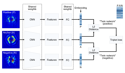
Figure 1: The triplet network architecture for model training. Three input examples (anchor, positive and negative) are propagated through the triplet neural network simultaneously. Anchor and positive share the same label, thus forming a matching pair. In contrast, anchor and negative do not share the same label, thus forming an opposing pair. The three CNNs and FC layers share the same weights in the triplet network. After examples are embedded to a low dimensional vector space, a triplet loss function is used to simultaneously maximize similarities between matching embeddings and minimize those between opposing embeddings. A side-by-side comparison of three embeddings in a triplet are annotated at the upper right corner.

III-A The embedding model (the vision backbone)

Our embedding model consists of two convolutional layers that extract spatial features and two fully connected layers that compress these features into a low dimensional vector, or embedding. The detailed architecture of the embedding model is delineated in Fig. 2. The first convolutional layer uses a $5\times 5$ single channel filter with a stride of one and no padding. The second convolutional layer employs a 32-channel $5\times 5$ filter with a stride of one and no padding. A ReLU (rectified linear activation unit) activation function is applied to the outcome of each convolutional layer, which is followed by a batch normalization layer and a max-pooling operation performed by a $2\times 2$ filter with a stride of two. Then, two fully connected layers are used to generate the final embedding with the size of 128. This way, speckle patterns are encoded into embeddings in a low dimensional vector space, where the similarity of two embeddings can be evaluated by their squared $L2$ distance.

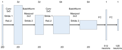
Figure 2: The network architecture of the embedding model. Each shaded rectangle is a volumetric data representation in the neural network pipeline. The channel number of each data representation is marked on the top row. The type of spatial dimension, such as 2D tensors or 1D tensor of neurons, is also annotated for each data representation at the bottom row. Notably, the initial spatial dimension of the input may change if cropping and resizing are applied.

III-B Triplet loss function

We train the embedding model in each twin neural network by using a triplet loss function described in (Schroff et al., 2015). Each input consists of a triplet of training examples, which are called anchor $x^{a}$, positive $x^{p}$ and negative $x^{n}$. Anchor has the same label as positive but not negative. Together, $(x^{a},x^{p})$ forms a matching pair, while $(x^{a},x^{n})$ forms an opposing pair. During training, three embedding models (CNN+FC) $f$ with shared weights map each element in a triplet $(x^{a},x^{p},x^{n})$ into a unified embedding vector space, respectively. The objective of training is to separate the two embeddings in each opposing pair by at least a margin of $\alpha$ from the embeddings in the corresponding matching pair in the vector space. Given $N$ triplets, the training objective can be stated as

$$\begin{array}[]{l}\|f(x_{i}^{a})-f(x_{i}^{p})\|_{2}^{2}+\alpha<\|f(x_{i}^{a})-f(x_{i}^{n})\|_{2}^{2},\,i=1\mathrel{{.}\,{.}}\nobreak N\end{array}$$ (1)

Meanwhile, we enforce that every embedding has a unit length of one in a $d$-dimensional vector space, namely $f(x)\in\mathbb{R}^{d}$ and $\|f(x)\|_{2}=1$. It means that any speckle pattern will be mapped to a single point on a $d$-dimensional hypersphere with the radius of one. The largest value of a possible $\alpha$ is 4 in the squared $L2$ norm sense.

To facilitate the training, the objective in Eq. (1) is turned into the triplet loss function in Eq. (2).

$$\sum_{i=1}^{N}\left[\alpha+\|f(x_{i}^{a})-f(x_{i}^{p})\|_{2}^{2}-\|f(x_{i}^{a})-f(x_{i}^{n})\|_{2}^{2}\right]_{+}$$ (2)

where $[\cdot]_{+}$ returns zero unless the input value is positive.

III-C Selection of semi-hard triplets

A triplet can be randomly selected in three steps: (1) Randomly choose a class; (2) Randomly sample two unique examples from the chosen class; (3) Randomly sample one example from any class other than the chosen class. This method, despite being easy to implement, might not deliver fast convergence when there are too many easy triplets. To explain it in detail, we consider three kinds of triplets that might exist during model training: easy, semi-hard and hard, as shown in Fig. 3(a). In an easy triplet, the negative example is already separated by at least a margin of $\alpha$ than the positive example. In a hard triplet, the negative example is actually closer to the anchor than the positive example. In a semi-hard triplet, the negative example is farther away from the anchor than the positive example with a margin smaller than $\alpha$. The problem with easy triplets is that they contribute to zero in the triplet loss, and thus the model weights will be adjusted only according to other triplets, namely semi-hard and hard triplets. The problem with too many hard examples is that they mostly constitute only a small fraction of the whole population. If the optimization prioritizes separating them from their corresponding anchors, the loss function will more likely get stuck in some bad local minima. Therefore, selecting semi-hard triplets for training is important. This strategy does not mean to ignore hard examples at all. Instead, once a hard example is pulled into the semi-hard zone, optimization can further drive them into the easy zone. This allows majority of the negative examples to stay away from their anchor by a considerable margin $\alpha$. From a practical standpoint, the selection of semi-hard triplets is done at the mini-batch level, where our model randomly selects a triplet that satisfies the following condition.

$$\|f(x_{i}^{a})-f(x_{i}^{p})\|_{2}^{2}\;<\;\|f(x_{i}^{a})-f(x_{i}^{n})\|_{2}^{2}\;<\;\|f(x_{i}^{a})-f(x_{i}^{p})\|_{2}^{2}+\alpha,$$ (3)

$$i=1\mathrel{{.}\,{.}}\nobreak N$$

However, complexity arises with semi-hard selections involving multiple single-particle samples. We choose to select random anchor $x^{a}$ and positive $x^{p}$ from the same sample with the same label, with the negative $x^{n}$ selected from any sample with a different label. Under this selection scheme, we lay out all scenarios for semi-hard selections when two unique single-particle samples (Particle X and Particle Y) are present, as shown in Fig. 3(b).

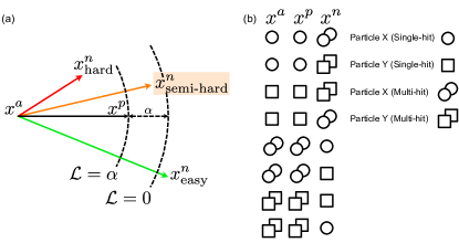
Figure 3: An illustration of the three types of negative examples. (a) $x^{a}$ represents an anchor example and $x^{p}$ is a positive example. Two arcs in dashed lines, both centered at $x^{a}$, are used to divide the embedding space into three areas. The inner arc has a radius of $\|f(x_{i}^{a})-f(x_{i}^{p})\|_{2}^{2}$, whereas the outer arc has a radius that is larger by a margin of $\alpha$. Negative examples will possess three difficulty levels in model training based on the area where they are situated. It is considered hard negative example if it is located within the inner arc, where $\|f(x_{i}^{a})-f(x_{i}^{n})\|_{2}^{2}<\|f(x_{i}^{a})-f(x_{i}^{p})\|_{2}^{2}$. On the contrary, it is considered an easy negative example when it goes outside the outer arc, where $\|f(x_{i}^{a})-f(x_{i}^{n})\|_{2}^{2}-\|f(x_{i}^{a})-f(x_{i}^{p})\|_{2}^{2}>\alpha$. Lastly, it becomes a semi-hard negative example when it resides in the area bound between the two arcs. Moreover, the loss function results in $\mathcal{L}=\alpha$ and $\mathcal{L}=0$ when $x^{n}_{\text{semi-hard}}$ is on the inner arc and outer arc, respectively. Our model training will pull $x^{n}_{\text{semi-hard}}$ close to the outer arc as much as possible, namely minimizing the loss. (b) An illustration of possible semi-hard scenarios when two unique single-particle samples are involved.

III-D Optimization

We trained our neural network models using Adam (Kingma and Ba, 2017) with a learning rate of $10^{-3}$. The model weights are initialized to random values from a Gaussian probability distribution with a mean of $0.0$ and a standard deviation of $0.2$.

III-E Data augmentation

Data augmentation is widely used in many machine learning tasks to address limitations imposed by expensive human-labeling and improve model performance. In essence, “a data-augmentation is worth a thousand samples" (Balestriero et al., 2022). We applied four data augmentation strategies to each speckle pattern in our dataset, including random in-plane rotation, random masking, random zooming and random shifting in both horizontal and vertical directions. Random in-plane rotation mimics the effect of single-particle rotation. Random masking covers some area of a speckle pattern with constant-value pixel intensities to be more robust to bad pixels and parasitic scattering. Random zooming and random shifting enforce the model to learn features independent of detector distance, X-ray wavelength, and X-ray beam center. These data augmentation strategies expand the data distribution for the model without manual labeling.

An important caveat when applying data augmentation is to partition the data into training set and test set before the augmentation. Otherwise, it will lead to “data leakage” as explained in (Kapoor and Narayanan, 2022). One consequence of “data leakage” is the deceptively good model predictive performance measured on a test set that already contains data augmented or “leaked” from the training set. In other words, the “good” performance will be mostly caused by model memorization or overfitting rather than generalization.

III-F Four steps in classification

Our model maps speckle patterns into a unified embedding space, without directly predicting labels. Instead, label prediction is performed in a query-against-support manner, that is, comparing inputs (queries) to labeled examples (supports). This approach is also referred to few-shot classification, often implying novel classes for queries and supports. In an $N$-way $X$-shot classification, $N$ is the number of classes and $X$ is the number of labeled examples per class. The classification takes four steps: (1) We embed an unknown input speckle pattern and all support examples in a unified embedding space. (2) We calculate the Euclidean distances from the input to every support example. (3) We average all distances by class. (4) We rank all classes by average distance and select the class with the shortest distance as the label of the unknown speckle pattern. Fig. 4 demonstrates an example of 2-way 5-shot classification.

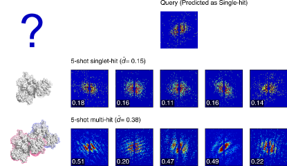
Figure 4: An illustration of a 2-way 5-shot classification. The speckle patterns in this figure are simulated from a type VI secretion system (PDB entry: 6N38). A queried speckle pattern is shown in the first row that has a ground truth label of single-hit. The second and third rows represent the single-hit and multi-hit support sets, respectively. 5 patterns are used in each support set. The query-to-support distance is annotated at the bottom left corner of each speckle pattern. The average query-to-support distance is denoted as $\bar{d}$. The single-hit class has a shorter $\bar{d}$ than the multi-hit class, resulting in a single-hit label for the query pattern. Additionally, a question mark in the first row indicates a to-be-determined label of a queried particle. To illustrate a single-hit example, we use a simple cartoon representation of a 6N38 molecule in the second row. Likewise, a multi-hit example is depicted by a cartoon representation of two 6N38 molecules with distinctly colored outlines.

IV Experiments

The ultimate goal of SpeckleNN is to accurately classify speckle patterns. Our unified embedding model facilitates the conversion of the speckle pattern classification problem into a set of similarity measures. Here we demonstrate two classification solutions, one with offline training and one with online training. Offline training requires past experimental data to train the model, which is then directly applied to classification of speckle patterns in future experiments. However, online training trains the model solely on newly collected data in an ongoing experiment. Both offline and online training are important for SPI experiments in high data rate facilities. Offline training offers a ready-to-use model for a wide range of samples, while online training provides a potentially more accurate experiment-specific model for the sample of interest.

As mentioned, training offline model requires speckle patterns from a variety of distinct samples. To this date, successful 3D reconstructions from single particle datasets are primarily from large viruses, such as mimivirus (Seibert et al., 2011), rice dwarf virus (Hajdu et al., 2016), and bacteriophage PR772 (Li, 2020). Therefore, we elected to demonstrate the offline-trained model on simulated data. Meanwhile, our model is designed to work on one sample of interest when trained online. We chose to use real bacteriophage PR772 data collected at LCLS for demonstration of model training and testing.

IV-A Offline training

IV-A1 Dataset

We randomly selected 100 Protein Data Bank (PDB) entries for model training and validation, and another 345 PDB entries for model testing. The number of atoms in those PDB entries ranges from $10^{4}$ to $10^{5}$. For every PDB entry, we simulated 400 speckle patterns, with 100 per hit category, from randomly oriented particles in the form of single-hit, double-hit, triple-hit and quadruple-hit. For training purposes, we keep the single-hit label but relabel the rest as multi-hit. The beam profile employed in the simulation has a radius of 0.5 $\mu m$ and a photon energy of 1.66 $keV$, and contains $10^{12}$ photons per pulse. We simulated all speckle patterns using skopi (Peck et al., 2022) on a square detector with a dimension of $172\times 172$ pixels. To replicate the conditions similar to real experiments, we firstly applied a $6\times 8$ pixel binary mask mimicking a beam stop at the center and another $172\times 4$ pixel binary mask resembling a gap dividing a detector in the middle. Then, X-ray fluence jitter and shot noise were introduced to the dataset. Specifically, during model training, we introduce fluence jitter by rescaling the intensity of speckle patterns with a multiplier sampled from an experimental photon number distribution shown in Fig. 5. We also added Gaussian noise with zero mean and 0.15 standard deviation. Each speckle pattern is also cropped at the center with a window size of $96\times 96$. Data augmentation described in the method section was applied subsequently.

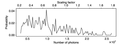
Figure 5: Probability distribution of photon numbers in 332 single-hit speckle patterns, obtained from LCLS experiment of bacteriophage PR772 at the AMO instrument (Experiment ID: amo06156, Run numbers: 90, 91, 94, 96 and 102) (Li, 2020). Dividing by mean photon numbers ($\approx 1.5\times 10^{7}$) produces scaling factors specified in the upper x-axis.

The speckle patterns simulated from the 100 PDB entries are split into $70\%$ for training and $30\%$ for validation. With data augmentation, we obtained $30,000$ speckle patterns for model training and another $10,000$ for model validation. We found applying data augmentation can add significant latency to the training process, so decided to cache all speckle patterns into CPU memory. But it is possible to pack even more data for model training through better practices, such as applying data augmentation to a new batch of data while training on the previous batch is still underway.

The test set was formed by simulating speckle patterns from 345 PDB entries. For model prediction, we generated $1,000$ speckle patterns for each PDB entry through random in-plane rotation as the only data augmentation strategy. The main reason is that speckle patterns aren’t subject to random masking, random shifting or random zooming as long as the experimental setup stays unchanged. We computed a confusion matrix for each PDB entry and reported accuracy and F-1 scores in the following results.

IV-A2 Performance and photon fluence

X-ray photon fluence jitter is often present in SPI speckle patterns. To illustrate how fluence jitter affects our model performance, we scanned a range of fluence scaling factors from $10^{-2}$ to $10^{2}$ by multiplying by $10^{0.5}$ at each step. These scaling factors are then applied to simulated speckle patterns in the test set. Meanwhile, we also measured model performance in three unique few-shot classification scenarios, including 1-shot, 5-shot and 20-shot. At the baseline photon fluence, our model achieves an average accuracy of 84.3%, 89.1% and 89.6% with 1-shot, 5-shot and 20-shot classification, respectively. The corresponding F-1 scores are 82.0%, 87.4% and 87.9%, respectively. Accuracy and F-1 scores both rise in response to the increase of photon fluence, and converge at about $10^{0.6}(\approx 4.0)\times$ the baseline photon fluence.

There are two main lessons we learned from this result. Firstly, the improvement in classification diminishes quickly with increase in support size. For example, 5-shot classification has a much better performance than 1-shot classification, but it delivers a comparable performance as 20-shot classification. If we were to deploy SpeckleNN at an undergoing experiment, it would be more appealing to only label 5 examples per category rather than 1 or 20 examples. Secondly, as free electron laser technology improves in peak brightness(Li et al., 2022), the benefit of having higher photon fluence can directly improve SpeckleNN’s accuracy. Interestingly, a $4\times$ photon fluence improvement is sufficient to maximize model performance.

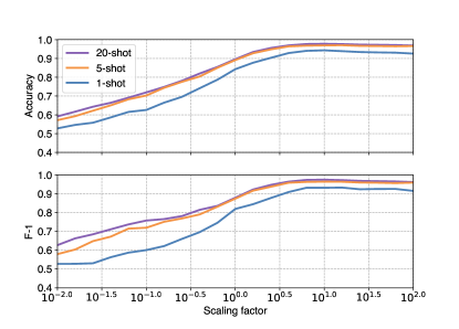
Figure 6: 2-way $X$-shot ($X=1,5,20$) classification performance of our model, as measured by accuracy and F-1 scores under a range of fluence conditions. The baseline fluence is $10^{12}$ photons per X-ray pulse.

IV-A3 Performance and particle size

PDB entries vary significantly in particle size from hundreds to millions of atoms, and their sizes are unevenly distributed. It is not a good practice to form a training dataset by randomly picking PDB entries, which might result in many entries aggregated within a small size range. Models trained on such dataset might perform well only on the highly populated size ranges but less so otherwise. We pick roughly equal number of PDB entries from 20 evenly spaced intervals from $10^{4}$ to $10^{5}$ atoms. The distribution of PDB entries over particle size used in our model training is visualized in Fig. 7(a). The PDB entries used in the test set were also sampled from the same size range.

We pointed out that particle size is a limiting factor in model prediction but conditioned on photon fluence. As shown in Fig. 7 (b), the average test accuracy of our model at the baseline photon fluence ($1\times$ condition) is positively correlated with particle size in the region of $1\times 10^{4}$ to $3\times 10^{4}$ atoms. The average test accuracy becomes stable when particle size is larger than $3\times 10^{4}$ despite the presence of outliers. Likewise, we repeated model prediction at $100\times$ larger photon fluence. No more size dependent correlation is observed across the whole size range, as shown in Fig. 7(c). Similar observation is also present in F-1 scores as shown in Fig. 7(d) and Fig. 7(e).

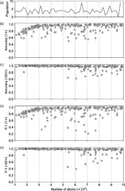
Figure 7: (a) The distribution of particle size, as characterized by the number of atoms, among PDB entries used in training the model. (b-e) 2-way 20-shot classification accuracy (b,c) and F-1 scores (d,e) plotted against number of atoms in each PDB entry under two respective fluence conditions, 1 $\times$ the baseline fluence and 100 $\times$ the baseline fluence. These conditions are labeled on the y-axes.

IV-B Online training

IV-B1 Dataset

We obtained speckle data from an LCLS experiment of bacteriophage PR772 collected at the AMO instrument (Experiment ID: amo06156, Run numbers: 90, 91, 94, 96 and 102) (Li, 2020). We prepared 332 single-hit, 165 multi-hit and 98 non-sample-hit patterns to form our source dataset. Non-sample-hit patterns do not exist in simulated data and are unique to experimental data, which are largely caused by parasitic scattering. We split data into 50% training set, 25% validation set and 25% test set. All speckle patterns were subject to data augmentation, specifically random rotation and random masking, from the source dataset. It is worth noting that we limit only 40 and 20 labeled examples per category for model training and validation, respectively. The purpose of imposing this restriction is to reproduce the shortage of labeled examples in a real experiment. However, we applied data augmentation to boost the number of examples per category. Consequently, there were 1374 non-sample-hit, 1288 single-hit and 1338 multi-hit patterns for model training, while there were 1359 non-sample-hit, 1352 single-hit and 1289 multi-hit patterns for model validation.

IV-B2 Robust classification despite missing detector area

To illustrate robust classification despite missing detector area, we need to choose a baseline model as a reference point for comparison. We decided to use (Shi et al., 2019)’s model for this purpose which we will refer to as Shi19 from here on out. It consists of a CNN vision backbone and a multi-layer perceptron (MLP) that outputs probabilities of each label. It reportedly achieved 83.8% accuracy in predicting single-hits. We reimplemented Shi19 model in PyTorch for measuring its performance. It is worth noting that we need to relabel non-sample-hit and multi-hit as non-single-hit to accommodate the training of Shi19 model, as it was initially designed for binary classification. We still used the original three labels to train our model, and only relabel them when producing compatible confusion matrices.

Performance comparison between models was conducted for two scenarios: (1) 100% detector area is available; (2) 25% detector area is available. The second scenario is more commonly seen in modular detectors, where certain area of the detector needs to be masked out due to spurious noise or damaged panels. Sometimes, data from some detector panels must be completely ignored to reduce computation time and thus allow rapid data collection. If speckle pattern classification can be accurately performed on only a fraction of a detector area, it opens the door to solving the “data reduction" problem that bottlenecks high-throughput single particle imaging experiments. That is to say, it can save a considerable amount of time by eliminating the need for assembling and calibrating all detector panels for the classification process.

Altogether, we randomly selected 345 single-hit and 655 non-single-hit speckle patterns to form the test set, with non-single-hit made up of 331 non-sample-hit and 324 multi-hit. SpeckleNN classifies speckle patterns in a 5-shot manner, whereas Shi19 model uses a probability threshold of 0.9 for the classification task. The model accuracy and F-1 scores are summarized in Table I. It is worth noting that data augmentation enhanced the accuracy of Shi19 model significantly, from 83.8% to 98% when 100% detector area is available. Meanwhile, under the same circumstances, SpeckleNN and Shi19 model have the same accuracy and F-1 scores, respectively. But SpeckleNN outperforms the competing model by a large margin when only 25% detector area is available. Fig. 8 and Fig. 9 are demonstrations of 3-way 5-shot classification with SpeckleNN on speckle patterns with 100% and 25% detector area available, respectively. This result suggests that SpeckleNN is a more robust speckle pattern classifier and thus better suited for high-throughput single particle imaging experiments.

TABLE I: Model accuracy (ACC) and F-1 scores in two scenarios: (1) 100% detector area is available; (2) 25% detector area is available. The percent detector area visibility is annotated as a subscript in the table. In addition, we performed 5-shot classification using SpeckleNN, and the probability threshold used in Shi19 model is 0.9.

Model	ACC100%	F-1100%	ACC25%	F-125%
SpeckleNN	0.98	0.97	0.94	0.92
Shi19 model	0.98	0.97	0.74	0.64

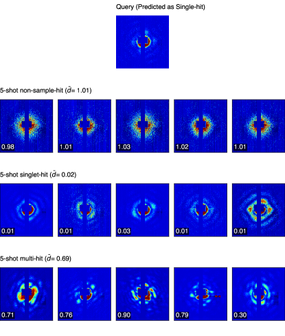
Figure 8: 3-way 5-shot classification on speckle patterns with 100% detector area available.

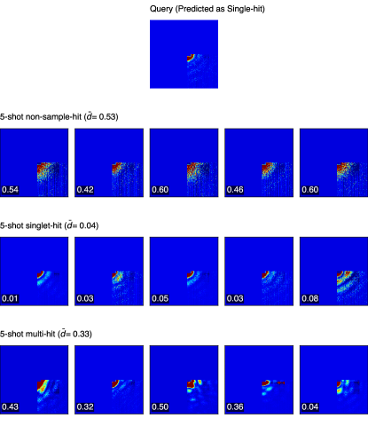
Figure 9: 3-way 5-shot classification on speckle patterns with 25% detector area available.

V Conclusions

In this work, we have introduced SpeckleNN, a unified embedding model for real-time speckle pattern classification in X-ray single particle imaging with limited labeled examples. The embedding model, trained with twin neural networks, can directly map speckle patterns to a unified vector space, where similarity is characterized by Euclidean distance. We have provided two distinct speckle pattern classification solutions. Firstly, the model trained on multiple samples offline allows few-shot classification of new never-seen single-particle samples. While our results show promising progress, future work is needed to transfer the model trained on simulated data to real experimental data. A more realistic simulator (Ledig et al., 2017) can potentially bridge this gap. Secondly, the model trained on one sample of interest online exhibits notably improved performance in the presence of substantial missing detector area, as compared to Shi19 model, a simple yet effective neural network based single-particle classifier. Our model’s ability to classify speckle patterns with partial detector information presents a significant opportunity for the development of a rapid speckle pattern vetoing process. Additionally, data augmentation is crucial in both offline and online training of our model, with a greater impact in online training.

References

- Andreasson et al. [2014] Jakob Andreasson, Andrew V. Martin, Meng Liang, Nicusor Timneanu, Andrew Aquila, Fenglin Wang, Bianca Iwan, Martin Svenda, Tomas Ekeberg, Max Hantke, Johan Bielecki, Daniel Rolles, Artem Rudenko, Lutz Foucar, Robert Hartmann, Benjamin Erk, Benedikt Rudek, Henry N. Chapman, Janos Hajdu, and Anton Barty. Automated identification and classification of single particle serial femtosecond X-ray diffraction data. Optics Express, 22(3):2497, February 2014. ISSN 1094-4087. doi: 10.1364/OE.22.002497.
- Aquila et al. [2015] A. Aquila, A. Barty, C. Bostedt, S. Boutet, G. Carini, D. dePonte, P. Drell, S. Doniach, K. H. Downing, T. Earnest, H. Elmlund, V. Elser, M. Gühr, J. Hajdu, J. Hastings, S. P. Hau-Riege, Z. Huang, E. E. Lattman, F. R. N. C. Maia, S. Marchesini, A. Ourmazd, C. Pellegrini, R. Santra, I. Schlichting, C. Schroer, J. C. H. Spence, I. A. Vartanyants, S. Wakatsuki, W. I. Weis, and G. J. Williams. The linac coherent light source single particle imaging road map. Structural Dynamics, 2(4):041701, July 2015. ISSN 2329-7778. doi: 10.1063/1.4918726.
- Ayyer et al. [2016] Kartik Ayyer, Ti-Yen Lan, Veit Elser, and N. Duane Loh. Dragonfly : An implementation of the expand–maximize–compress algorithm for single-particle imaging. Journal of Applied Crystallography, 49(4):1320–1335, August 2016. ISSN 1600-5767. doi: 10.1107/S1600576716008165.
- Balestriero et al. [2022] Randall Balestriero, Ishan Misra, and Yann LeCun. A Data-Augmentation Is Worth A Thousand Samples: Exact Quantification From Analytical Augmented Sample Moments, February 2022.
- Bobkov et al. [2015] S. A. Bobkov, A. B. Teslyuk, R. P. Kurta, O. Yu. Gorobtsov, O. M. Yefanov, V. A. Ilyin, R. A. Senin, and I. A. Vartanyants. Sorting algorithms for single-particle imaging experiments at X-ray free-electron lasers. Journal of Synchrotron Radiation, 22(6):1345–1352, November 2015. ISSN 1600-5775. doi: 10.1107/S1600577515017348.
- Bromley et al. [1993] Jane Bromley, James W. Bentz, Léon Bottou, Isabelle Guyon, Yann Lecun, Cliff Moore, Eduard Säckinger, and Roopak Shah. SIGNATURE VERIFICATION USING A “SIAMESE” TIME DELAY NEURAL NETWORK. International Journal of Pattern Recognition and Artificial Intelligence, 07(04):669–688, August 1993. ISSN 0218-0014, 1793-6381. doi: 10.1142/S0218001493000339.
- Chang et al. [2021] Hsing-Yin Chang, Elliott Slaughter, Seema Mirchandaney, Jeffrey Donatelli, and Chun Hong Yoon. Scaling and Acceleration of Three-dimensional Structure Determination for Single-Particle Imaging Experiments with SpiniFEL, September 2021.
- Chapman et al. [2006] Henry N. Chapman, Anton Barty, Michael J. Bogan, Sébastien Boutet, Matthias Frank, Stefan P. Hau-Riege, Stefano Marchesini, Bruce W. Woods, Saša Bajt, W. Henry Benner, Richard A. London, Elke Plönjes, Marion Kuhlmann, Rolf Treusch, Stefan Düsterer, Thomas Tschentscher, Jochen R. Schneider, Eberhard Spiller, Thomas Möller, Christoph Bostedt, Matthias Hoener, David A. Shapiro, Keith O. Hodgson, David van der Spoel, Florian Burmeister, Magnus Bergh, Carl Caleman, Gösta Huldt, M. Marvin Seibert, Filipe R. N. C. Maia, Richard W. Lee, Abraham Szöke, Nicusor Timneanu, and Janos Hajdu. Femtosecond diffractive imaging with a soft-X-ray free-electron laser. Nature Physics, 2(12):839–843, December 2006. ISSN 1745-2473, 1745-2481. doi: 10.1038/nphys461.
- Chopra et al. [2005] S. Chopra, R. Hadsell, and Y. LeCun. Learning a Similarity Metric Discriminatively, with Application to Face Verification. In 2005 IEEE Computer Society Conference on Computer Vision and Pattern Recognition (CVPR’05), volume 1, pages 539–546, San Diego, CA, USA, 2005. IEEE. ISBN 978-0-7695-2372-9. doi: 10.1109/CVPR.2005.202.
- Cruz-Chú et al. [2021] Eduardo R. Cruz-Chú, Ahmad Hosseinizadeh, Ghoncheh Mashayekhi, Russell Fung, Abbas Ourmazd, and Peter Schwander. Selecting XFEL single-particle snapshots by geometric machine learning. Structural Dynamics, 8(1):014701, January 2021. ISSN 2329-7778. doi: 10.1063/4.0000060.
- Donatelli et al. [2017] Jeffrey J. Donatelli, James A. Sethian, and Peter H. Zwart. Reconstruction from limited single-particle diffraction data via simultaneous determination of state, orientation, intensity, and phase. Proceedings of the National Academy of Sciences, 114(28):7222–7227, July 2017. ISSN 0027-8424, 1091-6490. doi: 10.1073/pnas.1708217114.
- Giannakis et al. [2012] Dimitrios Giannakis, Peter Schwander, and Abbas Ourmazd. The symmetries of image formation by scattering I Theoretical framework. Optics Express, 20(12):12799, June 2012. ISSN 1094-4087. doi: 10.1364/OE.20.012799.
- Hajdu et al. [2016] Janos Hajdu, Garth J. Williams, Changyong Song, Adrian Mancuso, Sébastien Boutet, Veit Elser, Andrew Aquila, Atsushi Nakagawa, Petra Fromme, Richard Kirian, Duane Loh, Anna Munke, Daniel Westphal, Raymond G. Sierra, Max F. Hantke, Nicusor Timneanu, Johan Bielecki, Kerstin Mühlig, Jakob Andreasson, Benedikt Daurer, Hemanth Kumar, Daniel S. D. Larsson, Filipe R. N. C Maia, Carl Nettelblad, Kenta Okamoto, Marvin Seibert, Martin Svenda, Gijs Van Der Schot, Salah Awel, Kartik Ayyer, Anton Barty, Max O. Wiedorn, Paulraj Lourdu Xavier, Richard J. Bean, Peter Berntsen, Hasan DeMirci, Akifumi Higashiura, Brenda Hogue, Yoonhee Kim, Ti-Yen Lan, Daewoong Nam, Garrett Nelson, Abbas Ourmazd, Max Rose, Peter Schwander, Ivan A. Vartanyants, Chun Hong Yoon, James Zook, Maximilian Bucher, Haiguang Liu, Henry Chapman, Ahmad Hosseinzadeh, and Jonas A. Sellberg. Coherent diffraction of single Rice Dwarf Virus particles using hard X-rays at the Linac Coherent Light Source. 2016. doi: 10.6084/M9.FIGSHARE.C.2342581.
- Hoffer and Ailon [2014] Elad Hoffer and Nir Ailon. Deep metric learning using Triplet network. 2014. doi: 10.48550/ARXIV.1412.6622.
- Ignatenko et al. [2021] Alexandr Ignatenko, Dameli Assalauova, Sergey A Bobkov, Luca Gelisio, Anton B Teslyuk, Viacheslav A Ilyin, and Ivan A Vartanyants. Classification of diffraction patterns in single particle imaging experiments performed at x-ray free-electron lasers using a convolutional neural network. Machine Learning: Science and Technology, 2(2):025014, June 2021. ISSN 2632-2153. doi: 10.1088/2632-2153/abd916.
- Kapoor and Narayanan [2022] Sayash Kapoor and Arvind Narayanan. Leakage and the Reproducibility Crisis in ML-based Science. arXiv, 2022. doi: 10.48550/ARXIV.2207.07048.
- Kingma and Ba [2017] Diederik P. Kingma and Jimmy Ba. Adam: A Method for Stochastic Optimization. arXiv:1412.6980 [cs], January 2017.
- Ledig et al. [2017] Christian Ledig, Lucas Theis, Ferenc Huszar, Jose Caballero, Andrew Cunningham, Alejandro Acosta, Andrew Aitken, Alykhan Tejani, Johannes Totz, Zehan Wang, and Wenzhe Shi. Photo-Realistic Single Image Super-Resolution Using a Generative Adversarial Network, May 2017.
- Li [2020] Haoyuan Li. Diffraction data from aerosolized Coliphage PR772 virus particles imaged with the Linac Coherent Light Source, 2020.
- Li et al. [2022] Haoyuan Li, James MacArthur, Sean Littleton, Mike Dunne, Zhirong Huang, and Diling Zhu. Femtosecond-Terawatt Hard X-Ray Pulse Generation with Chirped Pulse Amplification on a Free Electron Laser. Physical Review Letters, 129(21):213901, November 2022. ISSN 0031-9007, 1079-7114. doi: 10.1103/PhysRevLett.129.213901.
- Loh and Elser [2009] Ne-Te Duane Loh and Veit Elser. Reconstruction algorithm for single-particle diffraction imaging experiments. Physical Review E, 80(2):026705, August 2009. ISSN 1539-3755, 1550-2376. doi: 10.1103/PhysRevE.80.026705.
- Neutze et al. [2000] Richard Neutze, Remco Wouts, David van der Spoel, Edgar Weckert, and Janos Hajdu. Potential for biomolecular imaging with femtosecond X-ray pulses. Nature, 406(6797):752–757, August 2000. ISSN 0028-0836, 1476-4687. doi: 10.1038/35021099.
- Peck et al. [2022] Ariana Peck, Hsing-Yin Chang, Antoine Dujardin, Deeban Ramalingam, Monarin Uervirojnangkoorn, Zhaoyou Wang, Adrian Mancuso, Frédéric Poitevin, and Chun Hong Yoon. Skopi : A simulation package for diffractive imaging of noncrystalline biomolecules. Journal of Applied Crystallography, 55(4), August 2022. ISSN 1600-5767. doi: 10.1107/S1600576722005994.
- Reddy et al. [2017] Hemanth K.N. Reddy, Chun Hong Yoon, Andrew Aquila, Salah Awel, Kartik Ayyer, Anton Barty, Peter Berntsen, Johan Bielecki, Sergey Bobkov, Maximilian Bucher, Gabriella A. Carini, Sebastian Carron, Henry Chapman, Benedikt Daurer, Hasan DeMirci, Tomas Ekeberg, Petra Fromme, Janos Hajdu, Max Felix Hanke, Philip Hart, Brenda G. Hogue, Ahmad Hosseinizadeh, Yoonhee Kim, Richard A. Kirian, Ruslan P. Kurta, Daniel S.D. Larsson, N. Duane Loh, Filipe R.N.C. Maia, Adrian P. Mancuso, Kerstin Mühlig, Anna Munke, Daewoong Nam, Carl Nettelblad, Abbas Ourmazd, Max Rose, Peter Schwander, Marvin Seibert, Jonas A. Sellberg, Changyong Song, John C.H. Spence, Martin Svenda, Gijs Van der Schot, Ivan A. Vartanyants, Garth J. Williams, and P. Lourdu Xavier. Coherent soft X-ray diffraction imaging of coliphage PR772 at the Linac coherent light source. Scientific Data, 4(1):170079, December 2017. ISSN 2052-4463. doi: 10.1038/sdata.2017.79.
- Redmon and Farhadi [2016] Joseph Redmon and Ali Farhadi. YOLO9000: Better, Faster, Stronger. arXiv:1612.08242 [cs], December 2016.
- Redmon and Farhadi [2018] Joseph Redmon and Ali Farhadi. YOLOv3: An Incremental Improvement. arXiv, page 6, 2018.
- Schroff et al. [2015] Florian Schroff, Dmitry Kalenichenko, and James Philbin. FaceNet: A unified embedding for face recognition and clustering. In 2015 IEEE Conference on Computer Vision and Pattern Recognition (CVPR), pages 815–823, Boston, MA, USA, June 2015. IEEE. ISBN 978-1-4673-6964-0. doi: 10.1109/CVPR.2015.7298682.
- Schwander et al. [2012] Peter Schwander, Dimitrios Giannakis, Chun Hong Yoon, and Abbas Ourmazd. The symmetries of image formation by scattering II Applications. Optics Express, 20(12):12827, June 2012. ISSN 1094-4087. doi: 10.1364/OE.20.012827.
- Seibert et al. [2011] M. Marvin Seibert, Tomas Ekeberg, Filipe R. N. C. Maia, Martin Svenda, Jakob Andreasson, Olof Jönsson, Duško Odić, Bianca Iwan, Andrea Rocker, Daniel Westphal, Max Hantke, Daniel P. DePonte, Anton Barty, Joachim Schulz, Lars Gumprecht, Nicola Coppola, Andrew Aquila, Mengning Liang, Thomas A. White, Andrew Martin, Carl Caleman, Stephan Stern, Chantal Abergel, Virginie Seltzer, Jean-Michel Claverie, Christoph Bostedt, John D. Bozek, Sébastien Boutet, A. Alan Miahnahri, Marc Messerschmidt, Jacek Krzywinski, Garth Williams, Keith O. Hodgson, Michael J. Bogan, Christina Y. Hampton, Raymond G. Sierra, Dmitri Starodub, Inger Andersson, Saša Bajt, Miriam Barthelmess, John C. H. Spence, Petra Fromme, Uwe Weierstall, Richard Kirian, Mark Hunter, R. Bruce Doak, Stefano Marchesini, Stefan P. Hau-Riege, Matthias Frank, Robert L. Shoeman, Lukas Lomb, Sascha W. Epp, Robert Hartmann, Daniel Rolles, Artem Rudenko, Carlo Schmidt, Lutz Foucar, Nils Kimmel, Peter Holl, Benedikt Rudek, Benjamin Erk, André Hömke, Christian Reich, Daniel Pietschner, Georg Weidenspointner, Lothar Strüder, Günter Hauser, Hubert Gorke, Joachim Ullrich, Ilme Schlichting, Sven Herrmann, Gerhard Schaller, Florian Schopper, Heike Soltau, Kai-Uwe Kühnel, Robert Andritschke, Claus-Dieter Schröter, Faton Krasniqi, Mario Bott, Sebastian Schorb, Daniela Rupp, Marcus Adolph, Tais Gorkhover, Helmut Hirsemann, Guillaume Potdevin, Heinz Graafsma, Björn Nilsson, Henry N. Chapman, and Janos Hajdu. Single mimivirus particles intercepted and imaged with an X-ray laser. Nature, 470(7332):78–81, February 2011. ISSN 0028-0836, 1476-4687. doi: 10.1038/nature09748.
- Shi et al. [2019] Yingchen Shi, Ke Yin, Xuecheng Tai, Hasan DeMirci, Ahmad Hosseinizadeh, Brenda G. Hogue, Haoyuan Li, Abbas Ourmazd, Peter Schwander, Ivan A. Vartanyants, Chun Hong Yoon, Andrew Aquila, and Haiguang Liu. Evaluation of the performance of classification algorithms for XFEL single-particle imaging data. IUCrJ, 6(2):331–340, March 2019. ISSN 2052-2525. doi: 10.1107/S2052252519001854.
- Snell et al. [2017] Jake Snell, Kevin Swersky, and Richard S. Zemel. Prototypical Networks for Few-shot Learning. arXiv:1703.05175 [cs, stat], June 2017.
- Vinyals et al. [2017] Oriol Vinyals, Charles Blundell, Timothy Lillicrap, Koray Kavukcuoglu, and Daan Wierstra. Matching Networks for One Shot Learning, December 2017.
- Yoon et al. [2011] Chun Hong Yoon, Peter Schwander, Chantal Abergel, Inger Andersson, Jakob Andreasson, Andrew Aquila, Saša Bajt, Miriam Barthelmess, Anton Barty, Michael J. Bogan, Christoph Bostedt, John Bozek, Henry N. Chapman, Jean-Michel Claverie, Nicola Coppola, Daniel P. DePonte, Tomas Ekeberg, Sascha W. Epp, Benjamin Erk, Holger Fleckenstein, Lutz Foucar, Heinz Graafsma, Lars Gumprecht, Janos Hajdu, Christina Y. Hampton, Andreas Hartmann, Elisabeth Hartmann, Robert Hartmann, Gunter Hauser, Helmut Hirsemann, Peter Holl, Stephan Kassemeyer, Nils Kimmel, Maya Kiskinova, Mengning Liang, Ne-Te Duane Loh, Lukas Lomb, Filipe R. N. C. Maia, Andrew V. Martin, Karol Nass, Emanuele Pedersoli, Christian Reich, Daniel Rolles, Benedikt Rudek, Artem Rudenko, Ilme Schlichting, Joachim Schulz, Marvin Seibert, Virginie Seltzer, Robert L. Shoeman, Raymond G. Sierra, Heike Soltau, Dmitri Starodub, Jan Steinbrener, Gunter Stier, Lothar Strüder, Martin Svenda, Joachim Ullrich, Georg Weidenspointner, Thomas A. White, Cornelia Wunderer, and Abbas Ourmazd. Unsupervised classification of single-particle X-ray diffraction snapshots by spectral clustering. Optics Express, 19(17):16542, August 2011. ISSN 1094-4087. doi: 10.1364/OE.19.016542.
- Yoon [2012] Chunhong Yoon. Novel algorithms in coherent diffraction imaging using x-ray free-electron lasers. In Philip J. Bones, Michael A. Fiddy, and Rick P. Millane, editors, SPIE Optical Engineering + Applications, page 85000H, San Diego, California, USA, October 2012. doi: 10.1117/12.953634.