Robust Unsupervised StyleGAN Image Restoration

Abstract

GAN-based image restoration inverts the generative process to repair images corrupted by known degradations. Existing unsupervised methods must be carefully tuned for each task and degradation level. In this work, we make StyleGAN image restoration robust: a single set of hyperparameters works across a wide range of degradation levels. This makes it possible to handle combinations of several degradations, without the need to retune. Our proposed approach relies on a 3-phase progressive latent space extension and a conservative optimizer, which avoids the need for any additional regularization terms. Extensive experiments demonstrate robustness on inpainting, upsampling, denoising, and deartifacting at varying degradations levels, outperforming other StyleGAN-based inversion techniques. Our approach also favorably compares to diffusion-based restoration by yielding much more realistic inversion results. Code is available at the above URL.

1 Introduction

Image restoration, the task of recovering a high quality image from a degraded input, is a long-standing problem in image processing and computer vision. Since different restoration tasks—such as denoising, upsampling, deartifacting, etc.—can be quite distinct, many recent approaches [9, 10, 37, 61, 62, 54] propose to solve them in a supervised learning paradigm by leveraging curated datasets specifically designed for the task at hand. Unfortunately, designing task-specific approaches requires retraining large networks on each task separately.

In parallel, the advent of powerful generative models has enabled the emergence of unsupervised restoration methods [42], which do not require task-specific training. The idea is to invert the generative process to recover a clean image. Assuming a known (or approximate) degradation model, the optimization procedure therefore attempts to recover an image that both: 1) closely matches the target degraded image after undergoing a similar degradation model (fidelity); and 2) lies in the space of realistic images learned by the GAN (realism).

In the recent literature, StyleGAN [30, 31, 29] has been found to be particularly effective for unsupervised image restoration [40, 39, 15, 13, 14] because of the elegant design of its latent space. Indeed, these approaches leverage style inversion techniques [3, 4] to solve for a latent vector that, when given to the generator, creates an image close to the degraded target. Unfortunately, this only works when such a match actually exists in the model distribution, which is rarely the case in practice. Hence, effective methods extend the learned latent space to create additional degrees of freedom to admit more images; this creates the need for additional regularization losses. Hyperparameters must therefore carefully be tuned for each specific task and degradation level.

In this work, we make unsupervised StyleGAN image restoration-by-inversion robust to the type and intensity of degradations. Our proposed method employs the same hyperparameters across all tasks and levels and does not rely on any regularization loss. Our approach leans on two key ideas. First, we rely on a 3-phase progressive latent space extension: we begin by optimizing over the learned (global) latent space, then expand it across individual layers of the generator, and finally expand it further across individual filters—where optimization at each phase is initialized with the result of the previous one. Second, we rely on a conservative, normalized gradient descent (NGD) [58] optimizer which is naturally constrained to stay close to its initial point compared to more sophisticated approaches such as Adam [33]. This combination of prudent optimization over a progressively richer latent space avoids additional regularization terms altogether and keep the overall procedure simple and constant across all tasks. We evaluate our method on upsampling, inpainting, denoising and deartifacting on a wide range of degradation levels, achieving state-of-the-art results on most scenarios even when baselines are optimized on each independently. We also show that our approach outperforms existing techniques on compositions of these tasks without changing hyperparameters.

• We propose a robust 3-phase StyleGAN image restoration framework. Our optimization technique maintains: 1) strong realism when degradations level are high; and 2) high fidelity when they are low. Our method is fully unsupervised, requires no per-task training, and can handle different tasks at different levels without having to adjust hyperparameters.

• We demonstrate the effectiveness of the proposed method under diverse and composed degradations. We develop a benchmark of synthetic image restoration tasks—making their degradation levels easy to control—with care taken to avoid unrealistic assumptions. Our method outperforms existing unsupervised [40, 13] and diffusion-based [32] approaches.

2 Related work

This section covers previous work on StyleGAN inversion by optimization and its use for image restoration, and discusses related works on generative priors. Because the literature on general purpose image restoration is so extensive, we do not attempt to review it here and instead refer the reader to recent surveys [57, 35, 18, 19].

GANs and StyleGAN inversion

Generative adversarial networks [20] (GANs) are a popular technique for generative modeling. In particular, the StyleGAN family [30, 31, 28, 29] learns a highly compressed latent representation of its domain and stands out for its popularity and generation quality. Great progress has been made in StyleGAN inversion: reversing the generation process to infer latent parameters that generate a given image [59].

Thanks to inversion, StyleGAN has found use in many image editing [51, 23, 43] and restoration [40, 15, 14, 39, 13] tasks. Purely optimization-based techniques were studied extensively [3, 4, 26, 44, 66, 46] in the context of image editing. These methods extend the learned latent space of a pretrained StyleGAN model (commonly named $\mathcal{W}$) by adding additional parameters to optimize over it. The most common approach consists of using a different latent code for each layer [3] (dubbed $\mathcal{W}^{+}$). Going beyond $\mathcal{W}^{+}$ has also been explored in [46] who propose to fine-tune generator parameters, and [44] which uses different latent codes for each convolution filter. We build on these techniques by developing an inversion method designed specifically for robust image restoration.

Generative priors for unsupervised image restoration

Since the initial work of Bora et al. [6], multiple papers have used generative priors for unsupervised image restoration [25, 21]. Pan et al. [42] obtained high-resolution results with BigGAN [7]. They relax their latent inversion method by introducing a coarse-to-fine, layer-by-layer generator fine-tuning. Our method differs in that it addresses robustness and compositionality.

StyleGAN image restoration

Inversion methods designed for editing cannot be applied directly for restoration because loss functions are applied to degraded targets rather than clean images. Previous works address this with additional regularization terms and/or optimizer constraints. Of note, PULSE [40] proposed StyleGAN inversion for image upsampling, using a regularizer minimizing the latent extension to $\mathcal{W}^{+}$ and a spherical optimization technique on a Gaussian approximation of $\mathcal{W}$. While PULSE succeeds in preserving high realism, it obtains low fidelity when the downsampling factor is small. ILO [15] uses similar regularization techniques, and further extends the latent space by optimizing intermediate feature maps in a progressive fashion (layer-by-layer) while constraining the solutions to sparse deviations from the range. More recently, SGILO [14] proposes to replace this sparsity constraint and instead trains a score-based model to learn the distribution of the outputs of an intermediate layer in the StyleGAN generator. BRGM [39] frames GAN inversion as Bayesian inference and estimates the maximum a-posteriori over the input latent vector that generated the reconstructed image given different regularization constraints. Its followup, L-BRGM [13], jointly optimizes the $\mathcal{Z}$ (before the mapping network) and $\mathcal{W}$ spaces, further improving quality. In contrast, our work achieves robustness by avoiding any such regularization losses.

Other similar works

StyleGAN inversion was used to restore old photographs in [38]. Their method also restores a mixture of degradations, but is designed for real degradations (not robustness) and uses a task-specific encoder, while ours method is fully unsupervised. Multiple supervised methods [36, 34, 65, 56, 64, 22] focus on faces only, whereas our method does not use face-specific loss functions [16], is fully unsupervised, and works across a variety of image domains.

Diffusion models

Denoising diffusion probabilistic models (DDPMs) [53], trained on extremely large datasets (e.g., billions of images for [45, 49, 47]), have recently been shown to outclass GANs when it comes to image generation quality [17]. New approaches have been proposed to tackle image restoration using DDPMs, e.g., Palette [48] obtains excellent results by training the same model for several different tasks. Denoising diffusion restoration models (DDRM) [32] show that pretrained DDPMs can be used for unsupervised restoration tasks, but are limited to linear inverse problems with additive Gaussian noise. In contrast, our method is more flexible since it only requires a differentiable approximation of the degradation function, which can be non-linear.

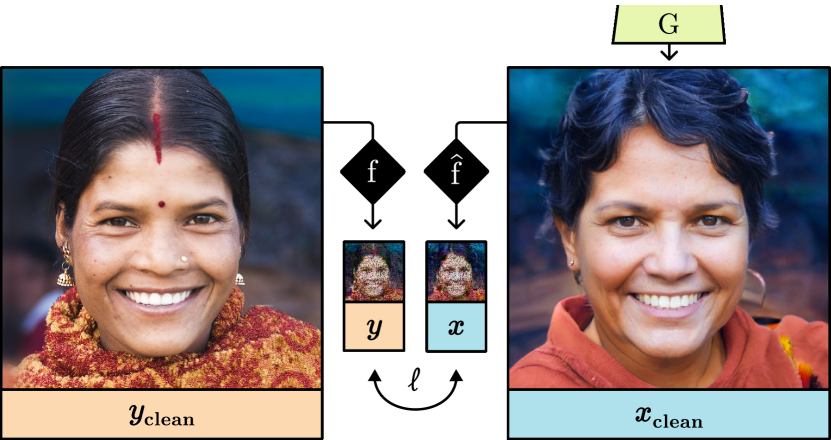
Figure 2: Unsupervised image restoration with StyleGAN attempts to restore a degraded target image $\boldsymbol{y}=f(\boldsymbol{y}_{\mathrm{clean}})$ by finding a generated image $\boldsymbol{x}_{\mathrm{clean}}$ that matches this target once also degraded $\boldsymbol{x}=\hat{f}(\boldsymbol{x}_{\mathrm{clean}})$ (sec. 3); here, $\hat{f}$ is a differentiable approximation to the degradation function $f$ and $\boldsymbol{y}_{\mathrm{clean}}$ is the (unknown) ground truth image.

3 Image restoration with StyleGAN

As illustrated in fig. 2, StyleGAN inversion attemps to recover an image $\boldsymbol{x}_{\mathrm{clean}}$ that best matches an (unknown) ground truth image $\boldsymbol{y}_{\mathrm{clean}}$. To this end, we aim to search for a latent code $\boldsymbol{w}\in\mathcal{W}$ such that $\boldsymbol{x}_{\mathrm{clean}}=G(\boldsymbol{w})$ best matches $\boldsymbol{y}_{\mathrm{clean}}$ under some image distance function $\ell$. The resulting minimization problem,

$$\boldsymbol{w}=\operatorname*{arg\,min}_{\tilde{\boldsymbol{w}}\in\mathcal{W}}\ell\big{(}G(\tilde{\boldsymbol{w}}),\boldsymbol{y}_{\mathrm{clean}}\big{)}\,,$$ (1)

can be solved by gradient descent. In image restoration, the ground truth image $\boldsymbol{y}_{\mathrm{clean}}$ is unknown: we are instead given a target image $\boldsymbol{y}=f(\boldsymbol{y}_{\mathrm{clean}})$, the result of a (non-injective, potentially non-differentiable) degradation function $f$. Assuming that a differentiable approximation $\hat{f}\approx f$ can be constructed, restoration is performed by solving for

$$\boldsymbol{w}=\operatorname*{arg\,min}_{\tilde{\boldsymbol{w}}\in\mathcal{W}}\ell\big{(}\hat{f}(G(\tilde{\boldsymbol{w}})),\boldsymbol{y}\big{)}\,.$$ (2)

This can be generalized to compositions of $k$ different degradations, i.e., $\{f_{i}\}_{i=1}^{k}$, by solving for

$$\boldsymbol{w}=\operatorname*{arg\,min}_{\tilde{\boldsymbol{w}}\in\mathcal{W}}\ell\big{(}[\hat{f}_{k}\circ...\circ\hat{f}_{2}\circ\hat{f}_{1}](G(\tilde{\boldsymbol{w}})),\boldsymbol{y}\big{)}\,,$$ (3)

where $\circ$ is the composition operator. Here, it is assumed that each subfunction $f_{i}$ has a differentiable approximation $\hat{f}_{i}$, and that the order of composition is known.

As described in sec. 2, this naïve approach finds solutions that have high realism (look like real faces), but low fidelity (do not match the degraded target). Fidelity is most commonly improved by 1) performing latent extension [3], that is, solving for $\boldsymbol{w}^{+}\in\mathcal{W}^{+}$ which has many more degrees of freedom; and 2) using a better performing optimizer like Adam [33]. These techniques both improve fidelity but also damage realism, motivating the use of regularization losses which must carefully be adjusted for different tasks [40, 39, 13]. In the next section, we show how the choice of latent extension and optimizer avoids the need for these regularizers.

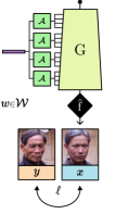
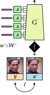
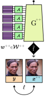
(a) Phase I	(b) Phase II	(c) Phase III

Figure 3: Our 3-phase latent extension (sec. 4.1) approach. (a) Phase I uses a global latent code $\boldsymbol{w}$, resulting in a prediction $\boldsymbol{x}$. (b) Phase II performs layer-wise latent expansion, resulting in matrix $\boldsymbol{w}^{+}$ and in a prediction $\boldsymbol{x}^{+}$. (c) Phase III performs filter-wise latent expansion, resulting in tensor $\boldsymbol{w}^{++}$ and the final prediction $\boldsymbol{x}^{++}$.

4 Robust StyleGAN inversion

We propose an inversion method designed specifically for robust image restoration, which revisits each aspect of the unsupervised StyleGAN optimization pipeline, namely latent extension, optimization, and loss functions.

4.1 Robust latent extension

Inspired by the intuition that initialization is the best regularization [46], we propose a three-phase latent extension, where each phase is initialized by the outcome of the previous one, see fig. 3. Given a pretrained StyleGAN2 [31] model with $N_{L}$ layers in the generator, we denote style vectors $\boldsymbol{s}^{l}_{i}\in\mathbb{R}^{512}$ at layer $l\in[1,N_{L}]$ used to modulate convolution weights $\boldsymbol{\theta}^{l}\in\mathbb{R}^{512\times 512}$. Assuming $1\times 1$ filters to simplify notation, each feature map pixel $\boldsymbol{p}^{l}\in\mathbb{R}^{512}$ is processed by

$$p^{l+1}_{i}=(\boldsymbol{\theta}^{l}_{i}\odot\boldsymbol{s}_{i}^{l})\boldsymbol{p}^{l}\,,$$ (4)

producing output feature $p^{l+1}_{i}\in\mathbb{R}$ where $i\in[0,512]$.

Phase I

performs global style modulation (fig. 3-(a)), and solves for a single latent vector $\boldsymbol{w}\in\mathcal{W}=\mathbb{R}^{512}$ shared across all layers as in eq. 3. Prior to optimization, $\boldsymbol{w}$ is initialized to the mean of $\mathcal{W}$ over the training set, i.e., $\mathbb{E}_{\tilde{\boldsymbol{w}}\in\mathcal{W}}[\tilde{\boldsymbol{w}}]$. Here, the style modulation vector $\boldsymbol{s}_{i}^{l}$ in eq. 4 can be written as

$$\boldsymbol{s}_{i}^{l}=\mathcal{A}^{l}(\boldsymbol{w})\,,$$ (5)

where $\mathcal{A}^{l}$ is the corresponding affine projection layer (which multiplies by a weight matrix and adds a bias).

Phase II

performs layer-wise latent extension [3] (fig. 3-(b)), and solves for a latent matrix $\boldsymbol{w}^{+}\in\mathcal{W}^{+}=\mathbb{R}^{N_{L}\times 512}$. Each row of $\boldsymbol{w}^{+}$ is initialized to $\boldsymbol{w}$. Style modulation for this phase becomes

$$\boldsymbol{s}_{i}^{l}=\mathcal{A}^{l}(\boldsymbol{w}^{+}_{l})\,.$$ (6)

Phase III

performs filter-wise latent extension (fig. 3-(c)), and solves for a latent tensor $\boldsymbol{w}^{++}\in\mathcal{W}^{++}=\mathbb{R}^{N_{F}\times N_{L}\times 512}$, where a different latent code is used for each convolution filter and where $N_{F}$ is the number of such filters. Each submatrix of $\boldsymbol{w}^{++}$ is initialized to $\boldsymbol{w}^{+}$. Style modulation for this phase becomes

$$\boldsymbol{s}_{i}^{l}=\mathcal{A}^{l}(\boldsymbol{w}_{i,l}^{++})\,.$$ (7)

Output: restored image $\boldsymbol{x}^{++}$

# Phase I

1 $\boldsymbol{w}=\mathbb{E}_{\tilde{\boldsymbol{w}}\in\mathcal{W}}[\tilde{\boldsymbol{w}}]$

2 for 1 to 150 do

3       $\boldsymbol{x}\leftarrow G(\boldsymbol{w})$

4       $\boldsymbol{w}\leftarrow 0.08\bar{\nabla}_{\boldsymbol{w}}\ell(\hat{f}(\boldsymbol{x}),\boldsymbol{y})$

5      

# Phase II

6 $\boldsymbol{w}^{+}=\mathrm{repeat}(\boldsymbol{w},N_{L})$

7 for 1 to 150 do

8       $\boldsymbol{x}^{+}\leftarrow G^{+}(\boldsymbol{w}^{+})$

9       $\boldsymbol{w}^{+}\leftarrow 0.02\bar{\nabla}_{\boldsymbol{w}}\ell(\hat{f}(\boldsymbol{x}^{+}),\boldsymbol{y})$

10      

# Phase III

11 $\boldsymbol{w}^{++}=\mathrm{repeat}(\boldsymbol{w}^{+},N_{F})$

12 for 1 to 150 do

13       $\boldsymbol{x}^{++}\leftarrow G^{++}(\boldsymbol{w}^{++})$

14       $\boldsymbol{w}^{++}\leftarrow 0.005\bar{\nabla}_{\boldsymbol{w}^{++}}\ell(\hat{f}(\boldsymbol{x}^{++}),\boldsymbol{y})$

15      

return $\boldsymbol{x}^{++}$

Algorithm 1 Robust StyleGAN inversion.

4.2 Robust optimization

While most inversion approaches use the Adam [33] optimizer to solve eq. 3, we instead propose coupling our 3-phase latent extension with a weaker optimizer, normalized gradient decent (NGD) [58], a simple variant of SGD that normalizes the gradient before each step:

$$\bar{\nabla}_{\boldsymbol{w}}\ell(\boldsymbol{w})=\frac{\nabla_{\boldsymbol{w}}\ell(\boldsymbol{w})}{||\nabla_{\boldsymbol{w}}\ell(\boldsymbol{w})||_{2}}\,,$$ (8)

Here, the gradient $\bar{\nabla}_{\boldsymbol{w}}\ell(\boldsymbol{w})$ is explicitly set to 0 when $||\nabla_{\boldsymbol{w}}\ell(\boldsymbol{w})||_{2}=0$. Following latent extension, we normalize each latent code separately (i.e. each row of $\boldsymbol{w}^{+}$ and $\boldsymbol{w}^{++}$). NGD conserves loss scale invariance, a key property of Adam that avoids learning rate adjustments following loss function changes.

4.3 Robust loss function

The staple loss function in StyleGAN inversion is the LPIPS [63] perceptual loss combined with a L2 or L1 [4] pixel-wise loss. We found a multiresolution loss function to be much more robust, and use:

$$\ell_{\mathrm{MR}}(\boldsymbol{x},\boldsymbol{y})=\sum_{i=1}^{k}\ell_{\mathrm{LPIPS}}(\phi(\boldsymbol{x},2^{i}),\phi(\boldsymbol{y},2^{i}))\,,$$ (9)

where $\phi(\cdot,2^{i})$ downsamples by a factor of $2^{i}$ using average pooling, and we set $k=6$ for image resolution of $1024^{2}$. All resolutions are weighted equally, giving our final loss function $\ell=\lambda_{\mathrm{L1}}\ell_{\mathrm{L1}}+\ell_{\mathrm{MR}}$ with $\lambda_{\mathrm{L1}}=0.1$.

4.4 Overall algorithm

Alg. 1 provides a detailed pseudo-code of our method. $G^{+}$ and $G^{++}$ denote the synthesis network $G$ after modification to accept $\boldsymbol{w}^{+}\in\mathcal{W}^{+}$ and $\boldsymbol{w}^{++}\in\mathcal{W}^{++}$, respectively. Hyperparameters like learning rates and number of steps are explicitly provided since they are held constant across all tasks. Their values were found by cross-validation on a subset of the FFHQ training set.

5 Benchmarking restoration robustness

This section first describes the proposed degradation models used in all experiments as well as their respective differentiable approximations. It then explains how compositions of tasks were formed.

5.1 Individual degradations

Experiments are performed on four common sources of image degradation: upsampling, inpainting, denoising, and deartifacting. Synthetic models are used to facilitate comparison at different degradation levels. Each degradation is tested at five levels, which are referred to as extra-small (XS), small (S), medium (M), large (L), and extra-large (XL). Parameters for each degradation level will be provided below for each task in that same order. Fig. 4 shows examples of all four degradations at the XS and XL levels, see supp.

Upsampling

targets $\boldsymbol{y}$ are produced by downsampling ground truth images $\boldsymbol{y}_{\mathrm{clean}}$ by integer factors $k_{\mathrm{down}}\in\{2,4,8,16,32\}$. Downsampling filters are uniformly sampled from the commonly used bilinear, bicubic, and Lanczos filters, which provides a coarse but broad range of aliasing profiles. During inversion, average pooling is used as the approximation $\hat{f}$ in all cases.

Inpainting

aims to predict missing regions in an image. To test a variety of masking conditions, random masks are generated by drawing $k_{\mathrm{strokes}}\in\{1,5,9,13,17\}$ random strokes of width $0.08r$ where $r$ is the image resolution, each stroke connecting two random points situated in the outer thirds of the image. In this task, $\hat{f}=f$ i.e. we assume that the mask is known. To avoid the bias introduced by black pixels when evaluating the LPIPS loss, identical noise of distribution $\mathcal{N}(0.5,1)$ is added to the masked region of both the prediction and the target before computing LPIPS.

Denoising

targets are generated by using a mixture of Poisson and Bernouilli noise, simulating common sources of noise in cameras, namely shot noise and dead (or hot) pixels respectively. This is a challenging scenario because unlike Gaussian noise, Poisson noise is non-additive and signal-dependent, while Bernouilli noise is biased. Additionally, both are non-differentiable. We used the parameters $k_{\mathrm{p}}\in\{96,48,24,12,6\}$ and $k_{\mathrm{b}}\in\{0.04,0.08,0.16,0.32,0.64\}$ where $k_{\mathrm{p}}$ gives the most likely value added to a pixel (independently for each channel) according to a Poisson distribution, and $k_{\mathrm{b}}$ the probability that all channels of a pixel are replaced with black. We also account for clamping during image serialization, resulting in the overall noise model:

$$\frac{\mathrm{clamp}(p^{\prime}\cdot m)}{255},\text{where}\,p^{\prime}\sim\mathcal{P}(k_{\mathrm{p}}p),m\sim\mathcal{B}(k_{\mathrm{b}})\,,$$ (10)

for a ground truth image pixel value $p\in[0.0,1.0]$ and where $\mathrm{clamp}(\cdot)$ saturates all values outside of $[0,255]$. Note that $p^{\prime}$ can only take discrete values. For the differentiable approximation $\hat{f}$, we replace the (non-differentiable, discrete) Poisson noise with a Gaussian approximation $\mathcal{N}(k_{\mathrm{p}}p-0.5,\sqrt{k_{\mathrm{p}}p})$ and treat the Bernoulli noise as an unknown mask. We also use a surrogate gradient for $\mathrm{clamp}$:

$$\frac{d}{dp}\mathrm{clamp}(p)\approx\frac{d}{dp}\mathrm{sigmoid}(2\cdot(p-0.5))\,.$$ (11)

Deartifacting

is performed on JPEG images compressed with libjpeg [2, 12] at quality levels $k_{\mathrm{jpeg}}\in\{18,15,12,9,6\}$. The lossy part of JPEG compression can be expressed as

$$\mathrm{quantize}\circ\mathrm{DCT}\circ\mathrm{to\_blocks}\circ\mathrm{chroma\_subsample}\,.$$ (12)

Here, 4:2:2 chroma subsampling is used. This final quantization step rounds each DCT component $c^{(k)}_{i,j}$ positioned in the $k^{\text{th}}$ block at indices $i,j$ with

$$\mathrm{quantize}(c^{(k)}_{i,j})=\lfloor c^{(k)}_{i,j}/Q_{i,j}\rceil\,,$$ (13)

where $Q_{i,j}\in[1,255]\subset\mathbb{N}$ is the corresponding value from the quantization table. Rounding is the only non-differentiable part of this chain (the lossless part of JPEG compression does not need to be differentiated). We read the quantization tables from file headers and use Lomnitz’s implementation [1] of [52], which proposes differentiable rounding:

$$\lfloor p\rceil\approx\lfloor p\rceil+(p-\lfloor p\rceil)^{3}\,.$$ (14)

We use this approximation to define a surrogate gradient (keeping the forward pass exact), and interpolate with a straight-through gradient estimator at $\alpha=0.8$:

$$\frac{d}{dp}\lfloor p\rceil\approx\frac{d}{dp}\Big{[}(1-\alpha)p+\alpha(p-\lfloor p\rceil)^{3}\Big{]}\,.$$ (15)

5.2 Composed degradations

Eq. 3 assumes knowledge of the order in which degradations are applied. In this work, the following restoration order is used:

$$\mathrm{inpaint}\circ\mathrm{deartifact}\circ\mathrm{denoise}\circ\mathrm{upsample}\,.$$ (16)

Task compositions are created with (subsequences of) this ordering. For example, upsampling and deartifacting form a composition of length 2. All compositions were formed with tasks at degradation level medium (M).

6 Comparison to StyleGAN-based methods

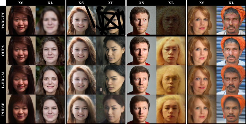
Figure 4: Randomly selected qualitative restoration results on each independent task, for both extra-small and extra-large levels of degradation. Top to bottom: (degraded) target, ours, L-BRGM [13], and PULSE [40]. Left to right: upsampling, inpainting, denoising, and deartifacting. Our method shows better robustness to variations in levels of degradation. See supp. for more results.

	Accur. (LPIPS) $\downarrow$				Fidelity (LPIPS) $\downarrow$				Realism (pFID) $\downarrow$
	PULS	L-BRG	OURS		PULS	L-BRG	OURS		PULS	L-BRG	OURS
Upsampling (bilinear, bicubic or Lanczos)
XS	.493	.407	.414		.432	.295	.313		44.5	23.6	17.0
S	.492	.412	.449		.353	.140	.239		34.3	25.5	22.0
M	.495	.458	.472		.261	.124	.172		29.3	35.4	22.3
L	.501	.487	.490		.185	.129	.127		21.9	26.0	20.9
XL	.512	.506	.514		.083	.095	.090		24.9	21.3	21.3
Denoising (clamped Poisson and Bernoulli mixture)
XS	.501	.440	.425		.275	.152	.156		56.1	27.2	18.5
S	.499	.450	.434		.252	.138	.140		53.7	28.6	19.1
M	.500	.465	.446		.224	.155	.130		54.5	22.1	19.8
L	.501	.481	.457		.185	.138	.110		56.4	24.6	19.2
XL	.504	.511	.474		.134	.110	.084		49.4	25.1	17.9
Deartifacting (JPEG compression)
XS	.498	.442	.432		.404	.341	.349		52.3	26.3	14.8
S	.497	.448	.437		.398	.352	.350		49.6	22.4	15.4
M	.498	.461	.445		.413	.357	.357		33.2	24.1	15.4
L	.500	.475	.460		.395	.367	.374		46.9	25.2	16.0
XL	.508	.503	.490		.427	.418	.412		30.8	22.1	18.7
Inpainting (random strokes)
XS	.498	.409	.378		.464	.374	.348		46.9	24.4	12.9
S	.501	.425	.387		.356	.287	.264		42.3	27.2	14.2
M	.509	.438	.396		.283	.227	.206		38.5	30.1	14.5
L	.513	.452	.409		.231	.184	.163		32.6	33.1	15.3
XL	.524	.460	.422		.187	.157	.132		36.2	25.2	15.9

Table 1: Quantitative comparison on individual tasks against baselines (“PULS” [40] and “L-BRG” [13]). Baselines are optimized for accuracy on each row separately, while ours uses the same set of hyperparameters across all. Despite this clear handicap, our method is either on par or outperforms baselines. Results color-coded as best and second best.

	Accur. (LPIPS) $\downarrow$				Fidelity (LPIPS) $\downarrow$				Realism (pFID) $\downarrow$
	PULS	L-BRG	OURS		PULS	L-BRG	OURS		PULS	L-BRG	OURS
2 degradations
NA	.517	.485	.459		.328	.301	.290		43.4	24.2	17.3
AP	.511	.478	.457		.270	.231	.204		29.7	17.6	17.0
UA	.510	.518	.508		.307	.348	.287		23.7	20.5	19.7
NP	.511	.480	.458		.125	.079	.062		47.0	20.9	19.2
UN	.501	.519	.511		.178	.149	.153		33.4	26.2	21.1
UP	.510	.478	.485		.140	.061	.089		23.9	35.3	20.7
3 degradations
UNP	.510	.526	.507		.086	.062	.051		28.5	22.1	20.1
UAP	.525	.523	.513		.205	.154	.119		23.0	18.4	20.5
UNA	.521	.535	.533		.265	.310	.290		26.2	20.7	22.8
NAP	.526	.502	.470		.210	.197	.160		38.7	18.4	18.5
4 degradations
UNAP	.533	.546	.525		.192	.177	.131		25.5	21.1	21.8

Table 2: Quantitative comparison on composed tasks (at medium levels) against baselines (“PULS” [40] and “L-BRG” [13]). Baselines are optimized for accuracy on each row separately, while ours uses the same set of hyperparameters across all. Despite this clear handicap, our method is either on par or outperforms baselines. Acronyms indicate restorations: Upsampling, deNoising, deArtifacting, and/or inPainting. Results color-coded as best and second best.

6.1 Models, datasets, and metrics

The PyTorch implementation [41] of StyleGAN2-ADA [28] is used in all experiments. In particular, we use the model pretrained on the FFHQ dataset [30] at $1024\times 1024$ resolution. Since the model is trained on the entire FFHQ dataset, we gathered an additional 100 test images, dubbed “FFHQ extras” (FFHQ-X), using the same alignment script. Overlap with FFHQ was avoided by filtering by date (see supp.).

Performance was measured via accuracy, realism, and fidelity metrics. Accuracy was measured with the LPIPS [63] between the predictions and the ground truth images. Realism was measured using the PatchFID [8] (pFID): FID [24] measured on image patches. More specifically, we extracted 1000 random crops of size $128\times 128$ per image, computing the FID of all crops from predictions to all crops from our FFHQ-X dataset. Finally, fidelity between degraded predictions and targets was measured using the LPIPS; this was done by degrading predictions with the true degradation to ignore the effect of differentiable approximations.

6.2 Baselines

Our method is compared on FFHQ-X against two unsupervised StyleGAN image restoration techniques, PULSE [40] and the current state of the art L-BRGM [13]. The same pretrained network is used for all approaches.

PULSE [40]

We adapted PULSE to use StyleGAN2-ADA and to tasks other than upsampling by increasing the number of steps from $100$ to $250$ and adjusting the learning rate to $0.8$ (manual inspection on validation data) to increase its robustness to novel tasks.

L-BRGM [13]

We adjust its learning rate $\lambda_{\mathrm{lr}}=0.05$ by manual inspection. L-BRGM uses best-of-$k$ random initialization; because initialization is difficult under high degradations, we doubled the number of samples from $100$ to $200$ and added a 0.8 truncation [30] to avoid outliers. L-BRGM also performs early stopping by inspecting the ground truth; for a fair comparison, we instead fixed the number of steps to $500$ as in BRGM [39].

Hyperparameter optimization for baselines

We optimize the accuracy metric for the baselines hyperparameters for each (task, level) pair individually directly on the FFHQ-X test set (see supp. for more details). In addition, baselines employ the ground truth Bernouilli mask (see sec. 5.1) in their differentiable approximation of eq. 10. Doing so was necessary for good performance.

Our method

We adjust hyperameters (learning rate and number of iterations, see alg. 1) once on validation data, then run our benchmark on the test set with no per-task or per-level hyperparameter adjustment: our method uses the same hyperparameters across all tasks and levels. Our method is not provided the Bernouilli mask. The total number of steps (450) is less than the 500 used for L-BRGM.

6.3 Experimental results

Robustness to degradation levels

Our benchmark is run on our FFQH-X test set (sec. 6.1) on all five levels of degradation for each individual task, and quantitative results are presented in tab. 1. Recall from sec. 6.2 that our method, which employs a single set of hyperparameters across all experiments, is pitted against baselines with hyperparameters optimized for each task and level individually. Despite this obvious impediment, our proposed method outperforms baselines in the vast majority of scenarios. In particular, it reaches better accuracy in the majority of tasks against baselines optimized for accuracy, and realism is strictly better. Fig. 4 illustrates the improved visual quality obtained with our method.

Robustness to compositions

Robustness to compositions of degradations was evaluated by forming all possible subsequences of degradations (order in eq. 16) at medium level. Quantitative results are aggregated in tab. 2, while fig. 5 presents qualitative examples. Our results show that both high fidelity and high realism are maintained with our method, while the baselines struggle under varied degradations.

Figure 5: Qualitative comparisons on all possible compositions of the four tasks given medium levels of degradation. Samples are chosen randomly, and acronyms indicate the degradations: Upsampling, inPainting, deNoising and/or deArtifacting (sec. 6.3).

Accur. (LPIPS) $\downarrow$			Realism (pFID) $\downarrow$
DDRM	OURS		DDRM	OURS
Exact Upsampling (known average pooling)
0.412	0.443		44.75	18.92
Inexact Upsampling (unknown nearest-neighbor)
0.559	0.539		67.06	32.81
Linear Denoising (additive Gaussian noise)
0.336	0.452		43.28	19.25
Nonlinear Denoising (clamped additive Gaussian noise)
0.530	0.450		156.1	19.06
Inpainting (masking random strokes)
0.289	0.301		26.12	25.71
Uncropping (top left corner unmasked)
0.468	0.418		34.33	17.645

Table 3: Quantitative comparison to DDRM [32] on accuracy and realism (see sec. 7). Results are color-coded as best.

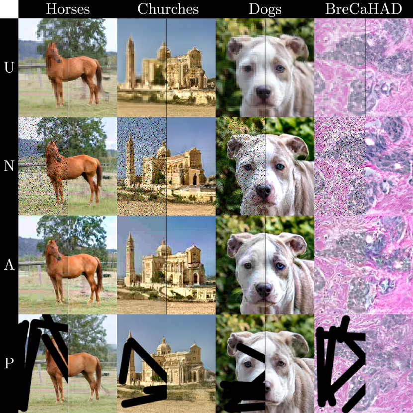
Figure 6: Results on LSUN horses and churches [60], AFHQ-v2 Dogs [11] and BreCaHAD [5] at resolution $256\times 256$ for small upsampling (U), small denoising (N), medium deartifacting (A), and medium inpainting (P); the left/right halves are the target/restored images. See supp. for details and more results.

7 Comparison to diffusion models

We compare our approach to the recent “Denoising diffusion restoration model” (DDRM) [32], which also does not require problem-specific supervised training and leverages a pre-trained (DDPM [53]) model. Importantly, DDRM is designed only for linear inverse problems with additive Gaussian noise, where the degradation model is perfectly known. Therefore, for each of the upsampling, denoising and inpainting tasks, we experiment with both: 1) a linear inverse problem with known parameters; and 2) an adjusted version which is either non-linear, where the extract degradation model is unknown, or a more extreme version of the problem. Specifically, we test: average pooling (known, linear) vs nearest-neighbor (unknown) $32\times$ (XL) upsampling; additive Gaussian noise (linear) vs clamped (to $[0,255]$) additive Gaussian noise (non-linear) with $\sigma^{2}=0.8$ (XL) for both; and masking strokes (at XL level) vs uncropping the top-left corner (XXL). DDRM is available on CelebA (not FFHQ) at $256\times 256$, so we use the corresponding StyleGAN2-ADA pretrained model. Due to the reduced resolution, pFID is measured on 250 patches of size $64\times 64$.

Interestingly, we find that DDRM reproduces the targets almost perfectly (fidelity is near zero, see supp. for details and qualitative results), to the point where it overfits to any deviation between its degradation model and the true degradation. Tab. 3 presents the accuracy and realism metrics for all the aforementioned tasks. While the accuracy favors DDRM for the tasks which perfectly match its assumptions, our approach outperforms it when this is not the case. In addition, our method provides significantly better realism across all scenarios. Overall, our approach yields high resolution results with more detail, can adapt to non-linear tasks, and it can also cope with larger degradations.

8 Discussion

Limitations

Our method is not restricted to faces and works with any pretrained StyleGAN, as demonstrated in fig. 6. However, it is inherently limited to the domain learned by the GAN. Training StyleGAN on a large unstructured dataset like ImageNet is difficult but recent papers [55, 50, 27] have attained some success—applying our method on some of these large-scale models is a promising research avenue. Our method also faces the same ethical considerations as the GAN it relies on. Finally, as with other methods [40, 13, 32], we also require knowledge of an (approximate) degradation function.

Conclusion

This paper presents a method which makes StyleGAN-based image restoration robust to both variability in degradation levels and to compositions of different degradations. Our proposed method relies on a conservative optimization procedure over a progressively richer latent space and avoids regularization terms altogether. Using a single set of hyperparameters, we obtain competitive and even state-of-the-art results on several challenging scenarios when compared to baselines that are optimized for each task/level individually.

Acknowledgements

This research was supported by NSERC grant RGPIN-2020-04799, a MITACS Globalink internship to Y. Poirier-Ginter, and by the Digital Research Alliance Canada.

References

- [1] Diffjpeg. https://github.com/mlomnitz/DiffJPEG.
- [2] Libjpeg. https://libjpeg-turbo.org.
- [3] Rameen Abdal, Yipeng Qin, and Peter Wonka. Image2StyleGAN: How to embed images into the StyleGAN latent space? In Int. Conf. Comput. Vis., 2019.
- [4] Rameen Abdal, Yipeng Qin, and Peter Wonka. Image2stylegan++: How to edit the embedded images? In IEEE Conf. Comput. Vis. Pattern Recog., 2020.
- [5] Alper Aksac, Douglas J Demetrick, Tansel Ozyer, and Reda Alhajj. Brecahad: a dataset for breast cancer histopathological annotation and diagnosis. BMC research notes, 12(1):1–3, 2019.
- [6] Ashish Bora, Ajil Jalal, Eric Price, and Alexandros G Dimakis. Compressed sensing using generative models. In Int. Conf. Mach. Learn., 2017.
- [7] Andrew Brock, Jeff Donahue, and Karen Simonyan. Large scale GAN training for high fidelity natural image synthesis. In Int. Conf. Learn. Represent., 2019.
- [8] Lucy Chai, Michael Gharbi, Eli Shechtman, Phillip Isola, and Richard Zhang. Any-resolution training for high-resolution image synthesis. In Eur. Conf. Comput. Vis., 2022.
- [9] Hanting Chen, Yunhe Wang, Tianyu Guo, Chang Xu, Yiping Deng, Zhenhua Liu, Siwei Ma, Chunjing Xu, Chao Xu, and Wen Gao. Pre-trained image processing transformer. In IEEE Conf. Comput. Vis. Pattern Recog., 2021.
- [10] Li-Heng Chen, Christos G Bampis, Zhi Li, Andrey Norkin, and Alan C Bovik. Proxiqa: A proxy approach to perceptual optimization of learned image compression. IEEE Trans. Image Process., 30:360–373, 2020.
- [11] Yunjey Choi, Youngjung Uh, Jaejun Yoo, and Jung-Woo Ha. Stargan v2: Diverse image synthesis for multiple domains. In IEEE Conf. Comput. Vis. Pattern Recog., 2020.
- [12] Alex Clark. Pillow (pil fork) documentation, 2015.
- [13] Arthur Conmy, Subhadip Mukherjee, and Carola-Bibiane Schönlieb. Stylegan-induced data-driven regularization for inverse problems. In Int. Conf. Acous. Sp. Sig. Proc., 2022.
- [14] Giannis Daras, Yuval Dagan, Alexandros G Dimakis, and Constantinos Daskalakis. Score-guided intermediate layer optimization: Fast Langevin mixing for inverse problems. In Int. Conf. Mach. Learn., 2022.
- [15] Giannis Daras, Joseph Dean, Ajil Jalal, and Alexandros G Dimakis. Intermediate layer optimization for inverse problems using deep generative models. In Int. Conf. Mach. Learn., 2021.
- [16] Jiankang Deng, Jia Guo, Niannan Xue, and Stefanos Zafeiriou. Arcface: Additive angular margin loss for deep face recognition. In IEEE Conf. Comput. Vis. Pattern Recog., 2019.
- [17] Prafulla Dhariwal and Alexander Nichol. Diffusion models beat gans on image synthesis. In Adv. Neural Inform. Process. Syst., 2021.
- [18] Omar Elharrouss, Noor Almaadeed, Somaya Ali Al-Maadeed, and Younes Akbari. Image inpainting: A review. Neural Processing Letters, 51:2007–2028, 2019.
- [19] Linwei Fan, Fan Zhang, Hui Fan, and Cai ming Zhang. Brief review of image denoising techniques. Visual Computing for Industry, Biomedicine and Art, 2, 2019.
- [20] Ian Goodfellow, Jean Pouget-Abadie, Mehdi Mirza, Bing Xu, David Warde-Farley, Sherjil Ozair, Aaron Courville, and Yoshua Bengio. Generative adversarial nets. In Adv. Neural Inform. Process. Syst., 2014.
- [21] Jinjin Gu, Yujun Shen, and Bolei Zhou. Image processing using multi-code gan prior. In IEEE Conf. Comput. Vis. Pattern Recog., 2020.
- [22] Yuchao Gu, Xintao Wang, Liangbin Xie, Chao Dong, Gen Li, Ying Shan, and Ming-Ming Cheng. Vqfr: Blind face restoration with vector-quantized dictionary and parallel decoder. In Eur. Conf. Comput. Vis., 2022.
- [23] Erik Härkönen, Aaron Hertzmann, Jaakko Lehtinen, and Sylvain Paris. Ganspace: Discovering interpretable gan controls. In Adv. Neural Inform. Process. Syst., 2020.
- [24] Martin Heusel, Hubert Ramsauer, Thomas Unterthiner, Bernhard Nessler, and Sepp Hochreiter. GANs trained by a two time-scale update rule converge to a local nash equilibrium. In Adv. Neural Inform. Process. Syst., 2017.
- [25] Shady Abu Hussein, Tom Tirer, and Raja Giryes. Image-adaptive gan based reconstruction. In Ass. Adv. Artif. Intel., 2020.
- [26] Kyoungkook Kang, Seongtae Kim, and Sunghyun Cho. Gan inversion for out-of-range images with geometric transformations. In Int. Conf. Comput. Vis., 2021.
- [27] Minguk Kang, Jun-Yan Zhu, Richard Zhang, Jaesik Park, Eli Shechtman, Sylvain Paris, and Taesung Park. Scaling up GANs for text-to-image synthesis. In IEEE Conf. Comput. Vis. Pattern Recog., 2023.
- [28] Tero Karras, Miika Aittala, Janne Hellsten, Samuli Laine, Jaakko Lehtinen, and Timo Aila. Training generative adversarial networks with limited data. In Adv. Neural Inform. Process. Syst., 2020.
- [29] Tero Karras, Miika Aittala, Samuli Laine, Erik Härkönen, Janne Hellsten, Jaakko Lehtinen, and Timo Aila. Alias-free generative adversarial networks. In Adv. Neural Inform. Process. Syst., 2021.
- [30] Tero Karras, Samuli Laine, and Timo Aila. A style-based generator architecture for generative adversarial networks. In IEEE Conf. Comput. Vis. Pattern Recog., 2019.
- [31] Tero Karras, Samuli Laine, Miika Aittala, Janne Hellsten, Jaakko Lehtinen, and Timo Aila. Analyzing and improving the image quality of StyleGAN. In IEEE Conf. Comput. Vis. Pattern Recog., 2020.
- [32] Bahjat Kawar, Michael Elad, Stefano Ermon, and Jiaming Song. Denoising diffusion restoration models. In Adv. Neural Inform. Process. Syst., 2022.
- [33] Diederik P Kingma and Jimmy Ba. Adam: A method for stochastic optimization. arXiv preprint arXiv:1412.6980, 2014.
- [34] Aijin Li, Gengyan Li, Lei Sun, and Xintao Wang. Faceformer: Scale-aware blind face restoration with transformers. ArXiv, abs/2207.09790, 2022.
- [35] Juncheng Li, Zehua Pei, and Tieyong Zeng. From beginner to master: A survey for deep learning-based single-image super-resolution. arXiv preprint arXiv:2109.14335, 2021.
- [36] Xiaoming Li, Wenyu Li, Dongwei Ren, Hongzhi Zhang, Meng Wang, and Wangmeng Zuo. Enhanced blind face restoration with multi-exemplar images and adaptive spatial feature fusion. In IEEE Conf. Comput. Vis. Pattern Recog., 2020.
- [37] Jingyun Liang, Jiezhang Cao, Guolei Sun, Kai Zhang, Luc Van Gool, and Radu Timofte. Swinir: Image restoration using swin transformer. In Int. Conf. Comput. Vis., 2021.
- [38] Xuan Luo, Xuaner Zhang, Paul Yoo, Ricardo Martin-Brualla, Jason Lawrence, and Steven M Seitz. Time-travel rephotography. ACM Trans. Graph., 40(6):1–12, 2021.
- [39] Razvan V Marinescu, Daniel Moyer, and Polina Golland. Bayesian image reconstruction using deep generative models. arXiv preprint arXiv:2012.04567, 2020.
- [40] Sachit Menon, Alexandru Damian, Shijia Hu, Nikhil Ravi, and Cynthia Rudin. Pulse: Self-supervised photo upsampling via latent space exploration of generative models. In IEEE Conf. Comput. Vis. Pattern Recog., 2020.
- [41] NVlabs. Stylegan2 ada - pytorch. https://github.com/NVlabs/stylegan2-ada-pytorch.
- [42] Xingang Pan, Xiaohang Zhan, Bo Dai, Dahua Lin, Chen Change Loy, and Ping Luo. Exploiting deep generative prior for versatile image restoration and manipulation. IEEE Trans. Pattern Anal. Mach. Intell., 2021.
- [43] Or Patashnik, Zongze Wu, Eli Shechtman, Daniel Cohen-Or, and Dani Lischinski. Styleclip: Text-driven manipulation of stylegan imagery. In Int. Conf. Comput. Vis., 2021.
- [44] Yohan Poirier-Ginter, Alexandre Lessard, Ryan Smith, and Jean-François Lalonde. Overparameterization improves StyleGAN inversion. In IEEE Conf. Comput. Vis. Pattern Recog., 2022.
- [45] Aditya Ramesh, Prafulla Dhariwal, Alex Nichol, Casey Chu, and Mark Chen. Hierarchical text-conditional image generation with clip latents. arXiv preprint arXiv:2204.06125, 2022.
- [46] Daniel Roich, Ron Mokady, Amit H Bermano, and Daniel Cohen-Or. Pivotal tuning for latent-based editing of real images. ACM Trans. Graph., 42(1), Feb. 2023.
- [47] Robin Rombach, Andreas Blattmann, Dominik Lorenz, Patrick Esser, and Björn Ommer. High-resolution image synthesis with latent diffusion models. In IEEE Conf. Comput. Vis. Pattern Recog., 2022.
- [48] Chitwan Saharia, William Chan, Huiwen Chang, Chris Lee, Jonathan Ho, Tim Salimans, David Fleet, and Mohammad Norouzi. Palette: Image-to-image diffusion models. ACM Trans. Graph., pages 1–10, 2022.
- [49] Chitwan Saharia, William Chan, Saurabh Saxena, Lala Li, Jay Whang, Emily Denton, Seyed Kamyar Seyed Ghasemipour, Burcu Karagol Ayan, S Sara Mahdavi, Rapha Gontijo Lopes, et al. Photorealistic text-to-image diffusion models with deep language understanding. arXiv preprint arXiv:2205.11487, 2022.
- [50] Axel Sauer, Katja Schwarz, and Andreas Geiger. StyleGAN-XL: Scaling stylegan to large diverse datasets. ACM Trans. Graph., 1, 2022.
- [51] Yujun Shen, Ceyuan Yang, Xiaoou Tang, and Bolei Zhou. Interfacegan: Interpreting the disentangled face representation learned by gans. IEEE Trans. Pattern Anal. Mach. Intell., 2020.
- [52] Richard Shin and Dawn Song. Jpeg-resistant adversarial images. In NeurIPS Workshop Mach. Learn. Comp. Sec., 2017.
- [53] Jascha Sohl-Dickstein, Eric Weiss, Niru Maheswaranathan, and Surya Ganguli. Deep unsupervised learning using nonequilibrium thermodynamics. In Int. Conf. Mach. Learn., 2015.
- [54] Zhengzhong Tu, Hossein Talebi, Han Zhang, Feng Yang, Peyman Milanfar, Alan Bovik, and Yinxiao Li. Maxim: Multi-axis MLP for image processing. In IEEE Conf. Comput. Vis. Pattern Recog., 2022.
- [55] Yuri Viazovetskyi, Vladimir Ivashkin, and Evgeny Kashin. Stylegan2 distillation for feed-forward image manipulation. In Eur. Conf. Comput. Vis., 2020.
- [56] Xintao Wang, Yu Li, Honglun Zhang, and Ying Shan. Towards real-world blind face restoration with generative facial prior. In IEEE Conf. Comput. Vis. Pattern Recog., 2021.
- [57] Zhihao Wang, Jian Chen, and Steven CH Hoi. Deep learning for image super-resolution: A survey. IEEE Trans. Pattern Anal. Mach. Intell., 43(10):3365–3387, 2020.
- [58] Jeremy Watt, Reza Borhani, and Aggelos K. Katsaggelos. Machine Learning Refined: Foundations, Algorithms, and Applications. Cambridge University Press, 2016.
- [59] Weihao Xia, Yulun Zhang, Yujiu Yang, Jing-Hao Xue, Bolei Zhou, and Ming-Hsuan Yang. GAN inversion: A survey. IEEE Trans. Pattern Anal. Mach. Intell., 2022.
- [60] Fisher Yu, Yinda Zhang, Shuran Song, Ari Seff, and Jianxiong Xiao. Lsun: Construction of a large-scale image dataset using deep learning with humans in the loop. arXiv preprint arXiv:1506.03365, 2015.
- [61] Syed Waqas Zamir, Aditya Arora, Salman Khan, Munawar Hayat, Fahad Shahbaz Khan, Ming-Hsuan Yang, and Ling Shao. Learning enriched features for real image restoration and enhancement. In Eur. Conf. Comput. Vis., 2020.
- [62] Syed Waqas Zamir, Aditya Arora, Salman Khan, Munawar Hayat, Fahad Shahbaz Khan, Ming-Hsuan Yang, and Ling Shao. Multi-stage progressive image restoration. In IEEE Conf. Comput. Vis. Pattern Recog., 2021.
- [63] Richard Zhang, Phillip Isola, Alexei A Efros, Eli Shechtman, and Oliver Wang. The unreasonable effectiveness of deep features as a perceptual metric. In IEEE Conf. Comput. Vis. Pattern Recog., 2018.
- [64] Shangchen Zhou, Kelvin CK Chan, Chongyi Li, and Chen Change Loy. Towards robust blind face restoration with codebook lookup transformer, 2022.
- [65] Feida Zhu, Junwei Zhu, Wenqing Chu, Xinyi Zhang, Xiaozhong Ji, Chengjie Wang, and Ying Tai. Blind face restoration via integrating face shape and generative priors. In IEEE Conf. Comput. Vis. Pattern Recog., 2022.
- [66] Peihao Zhu, Rameen Abdal, Yipeng Qin, John Femiani, and Peter Wonka. Improved stylegan embedding: Where are the good latents? arXiv preprint arXiv:2012.09036, 2020.