Parametric Differential Machine Learning for Pricing and Calibration

Abstract

Differential machine learning (DML) is a recently proposed technique that uses samplewise state derivatives to regularize least square fits to learn conditional expectations of functionals of stochastic processes as functions of state variables. Exploiting the derivative information leads to fewer samples than a vanilla ML approach for the same level of precision. This paper extends the methodology to parametric problems where the processes and functionals also depend on model and contract parameters, respectively. In addition, we propose adaptive parameter sampling to improve relative accuracy when the functionals have different magnitudes for different parameter sets. For calibration, we construct pricing surrogates for calibration instruments and optimize over them globally. We discuss strategies for robust calibration. We demonstrate the usefulness of our methodology on one-factor Cheyette models with benchmark rate volatility specification with an extra stochastic volatility factor on (two-curve) caplet prices at different strikes and maturities, first for parametric pricing, and then by calibrating to a given caplet volatility surface. To allow convenient and efficient simulation of processes and functionals and in particular the corresponding computation of samplewise derivatives, we propose to specify the processes and functionals in a low-code way close to mathematical notation which is then used to generate efficient computation of the functionals and derivatives in TensorFlow.

1 Introduction

In many financial applications, the goal is to compute the conditional expectation $E[Y|X]$, given $N_{S}$ joint samples $\{\left(X^{i},Y^{i}\right),i=1,...,N_{S}\}$ with $X^{i}=\left(X^{i}_{j},j=1,...,N_{X}\right)$ and $Y^{i}=\left(Y^{i}_{j},j=1,...,N_{Y}\right)$ where $N_{X}$ and $N_{Y}$ are the dimensions of $X$ and $Y$, respectively. Often, $X$ is a random input to some stochastic computation (or a random intermediate result of such computation) and $Y$ is the output of that computation. In particular, $X$ could be the initial (or intermediate) value of a stochastic process $S$ while $Y$ is a function of the final state of that process (or a functional of the full trajectory of that process).

Recently, machine learning techniques have been used to approximate $e(X)=E[Y|X]$ given enough joint samples of $X$ and $Y$. Let $N(X;\Theta_{N})$ denote a deep neural network (DNN) trained to approximate $e(X)$. Here, $\Theta_{N}$ denotes the trainable DNN parameters (typically weights and biases). The standard approach to train the best DNN is to minimize least squares as follows:

$$\Theta_{N}^{*,ML}=\underset{\Theta_{N}}{\arg\min}E\left[\left|Y-N(X;\Theta_{N})\right|^{2}\right],$$ (1)

resulting in $e^{*,ML}(X):=N\left(X;\Theta_{N}^{*,ML}\right)$. The standard approach is usually referred as vanilla ML approach in the literature. Recently, Huge and Savine [HS20a, HS20b] proposed a technique called Differential Machine Learning (DML) that uses information from sample-wise differentials to improve on the vanilla ML approach. Specifically, it minimizes least squares subject to regularization by derivatives as follows:

$$\Theta_{N}^{*,DML}=\underset{\Theta_{N}}{\arg\min}E\left[\left|Y-N(X;\Theta_{N})\right|^{2}+\sum_{i,j}\lambda_{ij}\left|DY_{ij}-\frac{\partial N(X;\Theta_{N})_{i}}{\partial X_{j}}\right|^{2}\right],$$ (2)

resulting in $e^{*,DML}(X):=N\left(X;\Theta_{N}^{*,DML}\right)$, where $DY_{ij}=\frac{\partial Y_{i}}{\partial X_{j}}$. In the case where conditional expectation and partial derivatives commute, the DML approach has the same optimal parameter sets as vanilla ML approach but can be learned more sample efficiently. In [HS20a, HS20b], Huge and Savine considered initial or intermediate states as input vector $X$ and final payoffs as output vector $Y$, and showed that for various financial instruments, the DML approach was more sample efficient than vanilla ML approach, especially with respect to approximation of derivatives.

We extend the DML technique to settings with parameters and call the technique Parametric Differential Machine Learning (PDML). The “parametric” in PDML comes from including parameters of the stochastic computation in $X$. When we consider functionals of stochastic processes, these could be model parameters for the stochastic process (for example, Heston parameters) or parameters related to the functional (for example, strike of (call) option) which we also call “contract parameters”. Using PDML technique we can learn efficient DNN surrogates to approximate conditional expectation (aka price of a financial instrument) as a function of model and/or contract parameters which can be used to either price several financial instruments simultaneously or to calibrate model parameters against market data of financial instruments. Here, note that efficient application of PDML requires efficient computation of partial derivatives of DNN surrogate $N(X;.)$ and output vector $Y$ wrt input vector $X$. In Section 2, we review how we obtain partial derivatives of DNN surrogate $N(X;.)$ wrt input vector $X$ via twin networks. This leaves the efficient computation of $\frac{\partial Y}{\partial X}$. Existing approaches typically involve the use of algorithmic differentiation or adjoint algorithmic differentiation (AD/AAD) techniques. Such AD/AAD approaches typically involve specifically prepared AD/AAD enabled source code which is then compiled and run in various modes, with the AAD system extracting and recording computational graphs, which are then used to compute derivatives. However, working with such approaches is often cumbersome and involved. A limited application domain such as simulation of a class of general stochastic processes and computation of functionals allows one to describe the computations to be performed (and differentiated) directly without executing them at first, to automatically generate the computations to be performed for any needed derivatives, and to run these computations for values and derivatives efficiently.

In Section 3, we describe a general set-up for these stochastic processes and functionals, how these stochastic prccesses and functionals can be specified by text input close to mathematical notation, and how the Python parser and TensorFlow 1 can be used to generate computational graphs for the computation of $Y$ and of $\frac{\partial Y}{\partial X}$. These computational graphs can be executed efficiently on CPU and GPU. In this way, we can efficiently and conveniently generate $Y$ and $\frac{\partial Y}{\partial X}$ for a large set of stochastic processes and functionals.

In Section 4, we describe the set-up for the PDML, the learning of surrogates, and parametric pricing. We will discuss in particular how to achieve good enough relative accuracy if magnitudes of prices for different parameter sets differ.

In Section 5, we introduce the model - Cheyette Model with benchmark rate volatility specification with an additional stochastic volatility factor, the instruments - two curve caplets, the parametric pricing setup, and parametric pricing results both for uniform and adaptive parameter sampling approaches. In Section 6, we discuss how to calibrate by optimizing on DNN surrogates for single maturity and multi-maturity settings with global optimization methods. We also discuss how random numbers in various parts of the pipeline impact the quality of the surrogates and the optimized parameters obtained from those surrogates. Finally, we discuss how to use that randomness, multiple seeds, and comparison to some ground truth indicators to obtain more robust calibration methods. In Section 7, we apply these calibration approaches and report promising results for both simple and robustified calibration methods for single maturity and multi-maturity settings. In Section 8, we conclude.

The parametric pricer developed by the PDML technique can compute prices and greeks for different financial instruments with different parmeter sets simultaneously, efficiently, and quickly. These parametric pricers allow much faster risk analytics computations of a portfolio of financial instruments and can be used as fast solvers inside a calibration approach.

Often, parametric pricing starts with specialized fast implementations of often simplified models reduced to a small number of factors since that parametric pricer will be called very often in the pricing and calibration setting, in particular repeatedly for each evaluation of the calibration objective function. Those specialized solvers and formulations for those models as well as appropriate simplifications need to be derived and implemented and are problem-specific. In the PDML demonstrated here, one only needs a differentiable implementation of the MC simulation and pricing under the original model. Instead of having to derive and implement each solver so that it fits within a particular API, we can construct such solvers based on input that looks very close to mathematical notation. The PDML technique results in DNN surrogates that can be very efficiently evaluated within the optimization and calibration loop so that now combining several surrogates and runs become feasible and the calibration can be further robustified. The proposed PDML technique gives promising results even as some of the components have not been separately optimized or adapted and thus further improvements are likely possible from future work.

2 Using DNNs to Represent Functions and Compute Derivatives

Deep neural networks (DNN) with nonlinear activation functions are universal function approximators, for a variety of architectures and some condition on the activation function. Modern deep learning frameworks, as for example TensorFlow and PyTorch, allow one to easily create and train DNNs of various architectures. One generally proceeds by specifying how one or several objective (“loss”) function(s) can be computed by (nontrainable) computations involving trainable DNNs and variables. In these frameworks, these computations are captured, either explicitly (as in TensorFlow 1 or TensorFlow 2’s TensorFlow 1 compatibility mode) or implicitly (by decorating and/or analyzing Python operations and functions), as computational graphs. The operations allowed in computations in these frameworks have efficiently implemented derivatives (both forward and adjoint) with respect to their arguments. Using these derivatives of the operations, these frameworks implement well known algorithmic differentiation techniques [Nau11] so that given the original computation, computations of appropriate derivatives can be easily added to the explicit or implicit computational graph.

Given these convenient and readily available frameworks, practioners have found that DNNs as parts of computational graphs are not only useful as theoretical constructs but show impressive results and efficient representations for a wide range of applications. The frameworks have implemented highly optimized computational infrastructure that can train on and evaluate such computational graphs and neural networks very efficiently on a wide range of computers and processors, from laptops over browsers running Google Colab notebooks on shared Google Colab resources to on-premises high-end multi-GPU and multi-core multi-CPU servers.

As an example, a fully connected feedforward DNN can be described by the equations [HS20a, Section 1.1.1], [HS20b]:

$$z_{0} = x$$

$$z_{l} = W_{l}\rho_{l-1}\left(z_{l-1}\right)+b_{l}=:\mathbf{FwdLayer}_{l}(z_{l-1},W_{l},b_{l})\quad,l=1,\ldots,L$$ (3)

$$y = z_{L}$$

where the $\rho$ are the activation functions, the $W$ are the (matrices with) weights, and the $b$ are the (vectors of) biases. The activation function of the first layer or the last layer or for the final result $y=\rho_{L}(z_{L})$ can be chosen differently than the ones for the middle layers. Typically, the same activation function is used for all middle layers. If there are constraints on the final output (such as that $y$ is supposed to be within a particular domain, such as positive, with a value between zero and one as for probabilities, or with components nonnegative and summing to one), these constraints can be enforced by a particular choice of activation function to be applied after the last layer, $y=\rho_{L}(z_{L})$, or in the last layer, $\rho_{L-1}$. If there are no such constraints, identity is a common choice for the last two activation functions.

We note that it is best practice to scale the inputs $x$ to DNNs and otherwise preprocess the input [HS20a]. Once determined, scaling can be implemented either before input is provided to the network, or as a particular first layer of the network with no or only some trainable elements. In particular cases, this can be implemented as a first layer with an identity activation function $\rho_{0}(x)=x$.

To demonstrate, Figure 1 shows the corresponding computational graph. Green circle nodes are inputs, gray circle nodes are outputs, pink circle nodes are trainable parameters (matrices and vectors), unfilled boxes are computations, and unfilled circle nodes are intermediate results.

Figure 1: Computational Graph for Feedforward Network

Neural networks are typically trained through back-propagation, a version of adjoint algorithmic differentiation adapted to the form of the networks, by proceeding backwards through the layers, as in:

$$\bar{z}_{L} = \bar{y}=1$$

$$\bar{z}_{l-1} = \left(\bar{z}_{l}W_{l}^{T}\right)\circ\rho_{l-1}^{\prime}\left(z_{l-1}\right)=:\mathbf{BwdLayer}_{l}({\bar{z}_{l}},z_{l-1},W_{l})\quad,l=L,\ldots,1$$ (4)

$$\bar{x} = \bar{z}_{0}$$

where the adjoint notation is used: $\bar{x}=\partial y/\partial x,\bar{z}_{l}=\partial y/\partial z_{l},\bar{y}=\partial y/\partial y=1$, $\circ$ is the elementwise product, and $\rho_{l}^{\prime}$ is the derivative of the activation function [HS20a, Section 1.1.2]. For this derivative to be smooth and make computational sense, the activation functions $\rho_{l}$ have to be differentiable, excluding the often used ReLU. However, there is a rather large variety of such activation functions including sigmoid, ELU, softplus, or swish.

At the end of the backward pass, $\bar{x}$ will contain the derivative of $y$ with respect to the input $x$. Just like the original network could be created easily in the framework, the second network computing the derivative of the network with respect to its input(s), can be created similarly, and one obtains a network that computes both the output and its derivative with respect to the input, in which the weights $W$ are shared between forward and backward network. This combined network is called “twin network” by Huge and Savine. We show in Figure 2 what nodes and computations are added to the forward network to also compute $\frac{\partial y}{\partial x}$ by adjoint algorithmic differentiation.

Figure 2: Computational Graph for Feedforward Network with Added Adjoint Computation of Derivative (“Twin network”)

Instead of explicitly implementing the backward network, one can also use the built-in functionalities of the framework to make the framework generate the computational graph for the and/or compute the specified derivatives. In TensorFlow, this is called tensorflow.gradient and adds operations to the computational graph to also compute the specified derivative, with respect to any input, parameter, or intermediate result specified.

In this way, we can easily obtain efficient implementations of the DNNs and of needed derivatives with respect to inputs and parameters.

To implement the forward mode of AD, one can extend the vectors so that they record both value and derivative of value with respect to input(s) and extend the operators so that they also correctly propagate the derivatives.

3 Differentiable Computation of Functionals of Simulated Stochastic Processes

3.1 General Setup

In quantitative finance applications, one very often has a description (model) that describes the dynamics of a number of risk factors or variables over time, say $S_{t}$ (vector, for a range of $t$), being started at $S_{0}$ (vector). This dynamics has parameters called model parameters ($\Theta_{S}$). Then, one or several payoffs - or other quantities of financial interest - are defined as functionals $F(S_{[0,T]})$ that in general can take the entire path between time 0 and time $T$ (the “maturity” or “computing time” of the payoff or quantity) as input and return one output. This functional can have parameters as well (“contract parameters”, $\Theta_{F}$). For example, consider an Asian call option in Black-Scholes model set-up:

$$dS_{t} = \mu S_{t}dt+\sigma S_{t}dW_{t},$$ (5)

$$F(S_{[0,T]}) = \left(\int_{0}^{T}S_{t}dt-K\right)^{+}.$$ (6)

Here, $\mu,\sigma$ are model parameters from $\Theta_{S}$ and $K$ is a contract parameter from $\Theta_{F}$.

In case of path-dependent functionals the entire path needs to be saved and processed which is considerably harder than working with functionals that depend on the state at one or several given ”fixing” times. So, for path-dependent functionals, one often looks for an exact or approximate markovianization by introducing an additional vector $U_{t}$ of “extra state” which turns the functional into a markovian functional $F^{U}$, i.e., $F^{U}(S_{T},U_{T}):=F(S_{[0,T]})$. For example, for an Asian call option, one possibility would be:

$$U_{t} = \int_{0}^{t}S_{s}ds,$$ (7)

$$F(S_{[0,T]}) = \left(U_{T}-K\right)^{+},$$ (8)

$$= F^{U}(S_{T},U_{T}).$$ (9)

Finally, $F(S_{[0,T]})$ respectively $F^{U}(S_{T},U_{T})$ is sampled and used for instance to estimate expectations or conditional expectations.

The further set-up now depends on the particular application. For instance, we are interested in parametric pricing of a fixed instrument assuming a given fixed starting state $S_{0}$. Under those circumstances, the input vector $X$ in the PDML setup from the introduction would be only the model parameters $\Theta_{S}$. Alternatively, one could try to learn a pricer across contract parameters also (varying strikes $K$, for instance, and then these contract parameters would be added as elements to $X$) and then use this to price a set of contracts of interest, such as calibration contracts. This is the parametric pricing set up that we will discuss here (including appropriate sensitivities).

Alternatively, for other applications, one could be interested in future values or pricing or exposures as of a certain time $T_{1}$, where $X$ would contain the future state $S_{T_{1}}$ (or $\left(S_{T_{1}},U_{T_{1}}\right)$ for the markovianized case). Here one could potential simulate the process up to time $T_{1}$ according to the same or some other dynamics or sample the $S_{T_{1}}$ (or $\left(S_{T_{1}},U_{T_{1}}\right)$ appropriately) and start the simulation at time $T_{1}$. This is the setting that Savine and Huge concentrate on. We will discuss such applications in future papers, but concentrate on parametric pricing here.

3.2 A General Class of Stochastic Processes and Functionals

In this section, we discuss the setup of system dynamics and its simulation. We begin with an assumption that we have specifications for a to-be-simulated/analyzed system as follows: Each component of the system is simulated or computed on some given time discretization grid either as

• A (presumably time-discretized) SDE/ODE with drift term (which can depend on all components and time) and volatility term(s) (which can depend on all components and time) associated with certain potentially correlated Brownian increments, with specified initial values (which could be fixed or generated according to some random distribution) OR

• A deterministic function of time and only already computed components at the same time OR

• A deterministic update function with specified initial values, whose next value is given as a function of its value at the previous time step, time corresponding to current time step, size of the current time step, potentially values of all other components at the previous time step, and values of only already computed components at the current time step.

The specification requires a set of potentially correlated Brownian increments. Correlations between any two (groups of) Brownian increments can be given as any functions of any components at the beginning of the corresponding time step.

With formulas, this looks as follows: Denoting component $i$ by $x^{i}$, allowing $K_{i}=0$ (in which case the sum is defined to be zero), allowing the drift functions to be zero, denoting ${\cal I}_{S}$ the indices for components given by SDEs or ODEs, ${\cal I}_{F}$ the indices for components given by functions, and $\mathsf{ind}(i,k)$ giving the index of the associated Brownian increment for the $k$th volterm for the $i$th component (volterms for different components can share the same Brownian increment), we have for the SDEs/ODEs, functions, and correlations of Brownians:

$$dx_{t}^{i} = \mathsf{drift}_{i}(t,(x_{t}^{j})^{M}_{j=1})dt+\sum_{k=1}^{K_{i}}\mathsf{vol}_{ik}(t,(x_{t}^{j})^{M}_{j=1})dW_{t}^{\mathsf{ind}(i,k)}\qquad(i\in{\cal I}_{S})$$ (10)

$$x_{t}^{i} = f_{i}(t,(x_{t}^{j})^{i-1}_{j=1})\qquad(i\in{\cal I}_{F})$$ (11)

$$\mathsf{corr}(dW_{t}^{i},dW_{t}^{j}) = \mathsf{correl}_{i,j}(t,(x^{k}_{t})^{M}_{k=1})$$ (12)

For any $i,j$ without given $\mathsf{correl}_{i,j}$ function, we use $\mathsf{correl}_{i,j}={1}_{i==j}$ (diagonal entries are one, off-diagonal entries are zero) to complete the specification so that trivial entries do not need to be given.

Update functions are defined on a discrete time grid with $t_{new}=t+\Delta t$ and ${\cal I}_{U}$ are the indices for components given by update functions:

$$x^{i}_{t_{new}}=\mathsf{upd}_{i}(t,\Delta t,(x^{j}_{t})^{M}_{j=1},(x^{j}_{t_{new}})^{i-1}_{j=1})\qquad(i\in{\cal I}_{U})$$ (13)

The sets of indices ${\cal I}_{S}$, ${\cal I}_{F}$, and ${\cal I}_{U}$ specify whether a given component is given as SDE (including ODE), markovian function, or update function.

Using Euler-Maruyama time-stepping, $\Sigma$ and $\Delta W$ being appropriate matrices and vectors, respectively, $N(.,.)$ being the normal distribution with a given mean vector and correlation matrix, we obtain:

$$\Sigma^{ij} = \mathsf{correl}_{i,j}(t,(x^{k}_{t})^{M}_{k=1})$$ (14)

$$\Delta W_{t} = \sqrt{\Delta t}N(0,\Sigma)$$ (15)

$$x^{i}_{t_{new}} = x_{t}^{i}+\mathsf{drift}_{i}(t,(x_{t}^{j})^{M}_{j=1})\Delta t+\sum_{k=1}^{K_{i}}\mathsf{vol}_{ik}(t,(x_{t}^{j})^{M}_{j=1})\Delta W_{t}^{\mathsf{ind}(i,k)}\qquad(i\in{\cal I}_{S})$$ (16)

$$x^{i}_{t_{new}} = f_{i}(t,(x^{j}_{t_{new}})^{i-1}_{j=1})\qquad(i\in{\cal I}_{F})$$ (17)

$$x^{i}_{t_{new}} = \mathsf{upd}_{i}(t,\Delta t,((x_{t}^{j})^{M}_{j=1},(x^{j}_{t_{new}})^{i-1}_{j=1})\qquad(i\in{\cal I}_{U})$$ (18)

This can also be interpreted by replacing differentials by differences (for $dx^{i}_{t}$ and $dt$) and by replacing Brownian increments $dW_{t}^{\mathsf{ind}(i,k)}$ by appropriately correlated normal random numbers $\Delta W_{t}^{\mathsf{ind}(i,k)}$ in the SDE/ODE expressions.

Finally, we intend to compute or estimate conditional expectations, which could be fully path-dependent and include a payoff $P$, a numeraire $\mathsf{Num}$, and/or a discount factor $\mathsf{DF}$

$$E\left[F(x_{[0:T]})|\cdot\right]=E\left[\frac{P(x_{[0:T]})}{\mathsf{Num}(x_{[0:T]})}|\cdot\right]=E\left[{P(x_{[0:T]})}{\mathsf{DF}(x_{[0:T]})}|\cdot\right],$$ (19)

or depend only on components at certain sampling times

$$E\left[\frac{P^{S}((x_{T_{k}})^{K}_{k=1})}{\mathsf{Num}^{S}((x_{T_{k}})^{K}_{k=1})}|\cdot\right]=E\left[{P^{S}((x_{T_{k}})^{K}_{k=1})}{\mathsf{DF}^{S}((x_{T_{k}})^{K}_{k=1})}|\cdot\right],$$ (20)

or could be completely markovian

$$E\left[\frac{P^{U}(x_{T})}{\mathsf{Num}^{U}(x_{T})}|\cdot\right]=E\left[{P^{U}(x_{T})}{\mathsf{DF}^{U}(x_{T})}|\cdot\right].$$ (21)

Our script framework discussed in Section 3.4 allows simple specification of the sampling times settings and markovian setting for the conditional expectations, with a syntax inspired by [SA21].

3.3 Conventional Approaches for Simulating Stochastic Processes and Computing Functionals and Their Derivatives

In most quantitative finance implementations of Monte-Carlo pricers, often models are implemented ad-hoc and one-off, with specialized implementations for each model, typically in C++, and then combined with appropriate payoffs for pricers, see [JJ04] for an introduction. To obtain differentiable implementations, one needs to write appropriately structured and prepared C++ code so that it can be combined with some Algorithmic (Adjoint) Differentiation (AD/AAD) framework or one’s own implementation of AAD, as discussed very well in [Sav18], including the modern use of Expression Templates.

Industry leading implementations have started to allow the user to describe payoffs in a script-like form, see [SA21], and process these scripts into object representations that can be used for simulation and pricing but also for more advanced applications such as computing CVA from the same script input.

However, we are not aware of any implementations in which the models (i.e., the stochastic processes) can be scripted and still be simulated efficiently.

Also, the preparation and maintenance of such appropriately structured C++ places a substantial burden on quantitative developers. Developers also need to use this instrumented code appropriately to extract, record, and process computational graphs (“tapes”) through their AAD frameworks. The framework is then used to compute needed derivatives based on those processed graphs, which requires additional care and burden. In the next subsection, we will discuss a much more convenient and automatic way to do so for the class of processes and functonals that we just described.

3.4 Script Framework for Simulating Stochastic Processes and Functionals

To the best of our knowledge, we are the first to implement model scripting. We started with a C++ framework and examined its usefulness for standard and hybrid models (see [Öge20, ÖGH20, ÖGH22, ÖH22]). This C++ framework allows the user to freely combine separately implemented sub-SDE systems, markovian updates, some functions and formulas, and payoffs. It was driven from Python input and enhanced by the Python interface. While very powerful, implementing completely new models required implementations of new classes. The use of AD/AAD frameworks allowed the computation of derivatives (albeit sometimes memory bound), but added complexity and maintenance burden, as discussed above.

For our current work, we are using a framework in which the system to be simulated is described in close-to-mathematical formulation, the Python parser is selectively used to generate appropriate abstract syntax trees and generate efficient implementations for TensorFlow and Numpy. Any necessary derivatives can be added in the TensorFlow implementation by standard TensorFlow capabilities.

As a first example, the input in Figure 3 specifies a log-Euler full truncation scheme for the Heston model to price a call option.

⬇

#system

d_logstock = (shortrate-0.5*variance)*d_t+volatility*d_Z

d_variance = kappa * (longtermvariance-positivepart(variance))*d_t \

+volofvol*volatility*d_W

volatility = sqrt(positivepart(variance))

#correlations

d_W*d_Z=rho

#initial values

init: logstock = initiallogspot

init: variance = initialvariance

#payoff

maturity: calloption pays (positivepart(exp(logstock[t])- strike)) \

discountby exp(-shortrate*t)

Figure 3: Script Input for Log-Euler Full Truncation Scheme for Call Option under Heston Model

The next listing in Figure 4 shows pricing of three call options: one on a continuous Asian average, one on a discrete Asian average, and an up-and-out barrier one with observation at each time step. The model is still Heston, but now treated with an Euler full truncation scheme. This listing also demonstrates some features including markovian updates for time-integral and maximum across time.

⬇

#system

d_stock = stock*(shortrate*d_t+volatility*d_Z)

d_stockint = stock * d_t

stockmax = max(stockmax,stock_new)

d_variance = kappa * (longtermvariance-positivepart(variance))*d_t \

+volofvol*volatility*d_W

volatility = sqrt(positivepart(variance))

#correlations

d_W*d_Z=rho

#initial values

init: stock = initialspot

init: stockmax = initialspot

init: variance = initialvariance

#payoff

maturity: asiancalloption pays (positivepart(stockint[t]- asianstrike)) \

discountby exp(-shortrate*t)

maturity: asiancalloption1 pays (positivepart(0.25*(stock[0.25*t]+\

stock[0.5*t]+\

stock[0.75*t]+\

stock[t])-asianstrike) \

discountby exp(-shortrate*t)

maturity: uocalloption pays (positivepart(stock[t]-strike) \

if (stockmax[t]<barrier) \

else zeroslike(stock[t])) \

discountby exp(-shortrate*t)

Figure 4: Script for Euler Full Truncation Scheme under Heston for Call Option on Continuous Asian Average, Call Option on Discrete Asian Average, and Up-and-Out Call Option with Barrier Observation at Each Time Step, Demonstrating Markovian Updates for Time-integral and Maximum.

As mentioned above, our Tensorflow backend is able to generate fully differentiable TensorFlow computational graphs from this input for the simulation of the system and the payoffs. For debugging, tests, and demonstrations, we also provide a Numpy backend for direct simulation of the system and payoffs under Numpy.

This framework has enabled us to very quickly and efficiently work with a wide range of models and payoffs based on relatively minimal input in a form close to mathematical notation.

4 Using PDML for Computing Conditional Expectations

4.1 Training of PDML Network Using Differentials wrt Parameters

As discussed in the introduction, there are various approaches to train DNNs for conditional expectations based on samples.

Without differential regularization, we obtain the “Vanilla ML” regression with loss function (see equation (1)):

$$\Theta_{N}^{*,ML}=\underset{\Theta_{N}}{\arg\min}E\left[\left|Y-N(X;\Theta_{N})\right|^{2}\right].$$

With complete differential regularization as in the introduction, we obtain the (P)DML regression with loss fuction (see equation (2)):

$$\Theta_{N}^{*,DML}=\underset{\Theta_{N}}{\arg\min}E\left[\left|Y-N(X;\Theta_{N})\right|^{2}+\sum_{i,j}\lambda_{ij}\left|DY_{ij}-\frac{\partial N(X;\Theta_{N})_{i}}{\partial X_{j}}\right|^{2}\right].$$

This regularization with the sample-wise differentials significantly improves the training and typically much fewer samples are needed for the same accuracy, even more so if a certain accuracy in derivative approximation is required. We use sample-wise differentials with respect to parameters (model, contract) and/or to state vector in training.

Sometimes, it is not necessary to include regularization with respect to all parameters or state features to achieve such improvement. Thus, we are using a setting where we allow partial differential regularization in the loss function:

$$\Theta_{N}^{*,PDML}=\underset{\Theta_{N}}{\arg\min}E\left[\left|Y-N(X;\Theta_{N})\right|^{2}+\sum_{i,j}\lambda_{ij}\left|DY_{ij}-\frac{\partial N(X;\Theta_{N})_{I(i)}}{\partial X_{J(j)}}\right|^{2}\right].$$ (22)

Here, $DY_{ij}=\frac{\partial Y_{I(i)}}{\partial X_{J(j)}}$. The mappings $I$ and $J$ specify which partial derivatives are used in the regularization.

The output $Y$ and sample-wise differentials $DY_{ij}$ are obtained from the script framework discussed in Section 3.4, which implements convenient derivatives with respect to parameters and initial or immediate state.

We then learn DNN with appropriate deep learning approaches according to the corresponding loss functions by minimization.

4.2 Learning the Surrogate

As discussed above, $X$ could contain varying parameters, initial values, intermediate values, or other inputs or outputs, coming from some simulated dynamics that could be started from fixed or varying initial values. $Y$ in general is a random variate – typically some output of a given computation – for which we want to compute a conditional expectation. For parameters and initial values, we are typically given ranges or domains, and we would pick particular values for the different realizations either by some deterministic scheme, quasi-random sampling, or random sampling according to some distributions.

For intermediate values and outputs, appropriate ranges and domains can sometimes only be determined from simulating and sampling, and it might be difficult to make sure that the simulated intermediate values and outputs appropriately cover the domain of interest. If the system can be markovianized and all state in $X$ is intermediate state at $t$, one could instead start simulation from an appropriately described and constrained markovian state $M_{t}$ at the intermediate time $t$ in question. Since in the setting in this paper, we do not condition on intermediate states, we will not discuss this further.

In case components of $X$ are parameters, initial values, or intermediate values which in the computational graph are connected with the output $Y$ and come before $Y$, adjoint algorithmic differentiation and appropriately prepared forward algorithmic differentiation can generate sample-wise derivatives of $Y$ with respect to those components of $X$. (If components of $X$ are outputs, one would need a reformulation or alternative approaches to compute partial derivatives of $Y$ with respect to those components of $X$. Since we are not handling this setting in this paper, we will not discuss this case further.)

We consider the case where components of $X$ are (dynamics or contract) parameters or potentially initial values. We generate computational graphs for the simulation and the computation of the functional(s). We will add nodes to the computational graph to compute derivatives with respect to some or all components of $X$ with the TensorFlow backend.

We will then generate vectors/tensors of appropriately deterministically or randomly sampled parameters and potentially initial values and we will then use the computational graph to generate simulations of system trajectories from appropriately randomly generated Brownian increments for the SDEs and compute samples of $Y$ and $DY$ for these trajectories. We typically generate all needed realizations in one run, but one could generate more realizations as needed, potentially adaptively.

We will specify the architecture of the surrogate DML network, such as a feedforward fully connected neural network with a certain number of hidden layers with a certain number of neurons each (but could use any other architecture that can be specified, initialized, and efficiently trained). Then, the weights, biases, or other trainable variables in the DML network have to be appropriately (randomly) initialized.

Then, we will use an appropriate optimization method to implement (2) (or (1) for VML). This could be a stochastic gradient method with momentum or other features, such as mini-batch ADAM [KB14], could be a more conventional gradient-based optimization with inexact or exact gradients such as L-BFGS, or could be optimization methods that treat the last layer explicitly by least-square methods as in [CGP⁺20, CGP⁺19]. In our work reported here, mini-batch SGD with ADAM with standard parameters seems to work well enough and so we leave more advanced methods to future work. Many of these optimization methods use random numbers.

Then, the optimization method is stoppped according to some stopping criterion, such as defined on changes to the parameters in the last optimization step, value of the objective function, or other considerations, and the resulting DML network is taken as surrogate. Given that we are using random numbers in several parts of the process, the final surrogate might vary with those random numbers and might be different and of different quality depending on the seed and other details of the random number generations.

This entire process can be wrapped into an appropriate module and pipeline.

4.3 Addressing Different Magnitudes for $Y$ for Different Parameters - Adaptive Sampling

If the $Y$ have all similar magnitude regardless of the parameter set, the above process will learn surrogates that fit the conditional expectation similarly well for parameters from different parts of the parameter domains. If the $Y$ vary in magnitude depending on the dynamics parameters, it turns out that DML surrogate will approximate the conditional expectations well for parameter settings for which the conditional expectations have the largest magnitude but not for parameters where the conditional expectations have smaller magnitudes. This is often not desirable.

There are many approaches to address this issue. For instance, one can sample the parameter regions resulting in smaller magnitude more intensively than others. To do this, one can first parametrically or nonparametrically estimate the magnitude of the $Y$ samples over the parameters and then construct marginal (or bivariate) parameter distributions resulting in approximately constant expectation of $Y$ across the parameter domain. This approach seems to work well in our implementations and tests and its results are reported below.

5 Pricing Setting and Results

We examine pricing of caplets under Cheyette models with one interest rate factor $x$ (and thus one auxiliary factor $y$) and with an additional stochastic volatility factor $z$. Furthermore, we consider benchmark rate volatility specifications for the “local” volatility. Floorlets can be priced very similarly. Caps and floors can be priced as sums of caplets and floorlets, respectively. In our future work, we will consider European swaptions and also Cheyette models with several interest rate factors.

5.1 Pricing Model: Cheyette Model

Here, we consider Cheyette models with a single interest rate factor with benchmark rate volatility specification [And01, AP10, Sch16]. Our benchmark forward rate is the forward rate for tenor $\delta$. In this type of Cheyette model, the benchmark instantaneous forward rate is given as:

$$f(t,t+\delta)=f(0,t)+h(\delta)\left(x_{t}+y_{t}G(\delta)\right),$$ (23)

where $h(\delta)=e^{-\kappa\delta}$ and $G(\delta)=\frac{1-h(\delta)}{\kappa}$ with $\kappa$ a given mean reversion.

The interest rate state $x_{t}$ and the auxiliary factor $y_{t}$ follow the following SDEs and ODEs under the risk neutral (bank account) measure:

$$dx_{t} = \left[y_{t}-\kappa x_{t}\right]dt+\sigma_{r}\left(t,x_{t},y_{t}\right)dW^{Q}_{t},$$ (24)

$$dy_{t} = \left[\sigma_{r}^{2}\left(t,x_{t},y_{t}\right)-2\kappa y_{t}\right]dt.$$ (25)

Both $x$ and $y$ start at 0 at $t=0$, $x_{0}\equiv 0$ and $y_{0}\equiv 0$.

Under the $T$-Forward measure, the SDE for $x(t)$ acquires an additional drift adjustment:

$$dx_{t}=\left[y_{t}-\kappa x_{t}-\sigma_{r}^{2}\left(t,x_{t},y_{t}\right)G(T-t)\right]dt+\sigma_{r}\left(t,x_{t},y_{t}\right)dW^{T}_{t}.$$ (26)

The “local” volatility term is given by

$$\textbf{(no SV)}:\sigma_{r}\left(t,x_{t},y_{t}\right) = h(\delta)\left[a(t)f(t,t+\delta)+b(t)\right],$$ (27)

$$\textbf{(SV)}:\sigma_{r}\left(t,x_{t},y_{t}\right) = \sqrt{z_{t}}h(\delta)\left[a(t)f(t,t+\delta)+b(t)\right],$$ (28)

which depends on $x_{t}$ and $y_{t}$ through (23).

In case of SV (stochastic volatility) setting, the dynamics of $z(t)$ is given by

$$dz_{t}=\theta\left[z_{0}-z_{t}\right]dt+\eta(t)\sqrt{z_{t}}dZ_{t},\hskip 5.69054ptz(0)\equiv z_{0}\equiv 1,\hskip 5.69054ptdZ_{t}dW^{Q(orT)}_{t}\equiv 0.$$ (29)

Under the Cheyette models under consideration, the discount factor curve as seen from time $t$ is given as:

$$P(t,T;x_{t},y_{t})=\frac{P(0,T)}{P(0,t)}\exp\left(-G(T-t)x_{t}-\frac{1}{2}G^{2}(T-t)y_{t}\right).$$ (30)

5.2 Instruments: (Two-Curve) Caplets

A caplet is an European style interest rate derivative. Let $T_{1}<T_{2}$, then the payoff of the caplet at $T_{2}$ for notional amount $N$ is

$$N\delta^{C}(T_{1},T_{2})\left(F_{T_{1}}^{F}\left(T_{1},T_{2}\right)-K\right)^{+},$$ (31)

where $K$ is the strike price, $F_{.}^{F}\left(T_{1},T_{2}\right)$ is the forward rate for the time period $\left[T_{1},T_{2}\right]$, $T_{1}$ is the reset date, $T_{2}$ is the payment date and $\delta^{C}$ is an appropriate day count fraction between $T_{1}$ and $T_{2}$ for the caplet payoff.

The forward rate can be computed from the discount factor for the forward/forecasting curve $P^{F}(t,T)$ - which represents the discount factor for $T$ as seen from $t$.

$$F_{t}^{F}\left(t^{S},t^{E}\right)=\frac{1}{\delta^{F}\left(t^{S},t^{E}\right)}\left(\frac{P^{F}\left(t,t^{S}\right)}{P^{F}\left(t,t^{E}\right)}-1\right),$$ (32)

with $\delta^{F}$ being the appropriate day count fraction for the forecasting forward rate.

We have given stochastic models for the two curves (forecasting and discounting curves) in the form of discount factor functions $P^{.}(t,T;\mathsf{state}_{t})$ where the $\mathsf{state}_{t}$ follows some stochastic process. In the Cheyette model under consideration, $\mathsf{state}_{t}=(x_{t},y_{t})$ (no SV) or $\mathsf{state}_{t}=(x_{t},y_{t},z_{t})$ (SV), but $P^{.}$ depends only on $(x_{t},y_{t})$ in both cases. We are using models such as the Cheyette model that reproduce the original curves so that $P^{.}(0,T;\mathsf{state}_{0})$ is equal to the curve $P^{.}(0,T)$ given as input.

5.2.1 Rewriting Two-Curve Payoffs into One-Curve Payoffs

Below, we will rewrite two-curve payoffs, in particular caplet payoffs, into one-curve payoffs. In the two-curve setting, forecasting curve $P^{F}$ and the discounting curve $P^{D}$ will be different. To be able to rewrite two-curve payoffs into one-curve payoffs, we will need to make sufficient assumptions about the relationship between the forecasting curve $P^{F}$ and the discounting curve $P^{D}$. One common such assumption is that these two curves have a deterministic multiplicative spread that does not change from the spread at time 0. This corresponds to hypothesis (S0) mentioned in [Hen10].

Define

$$\beta_{t}^{F}(u,v):=\frac{P^{F}(t,u)}{P^{F}(t,v)}\frac{P^{D}(t,v)}{P^{D}(t,u)}.$$ (33)

The deterministic multiplicative spread assumption corresponding to hypothesis S0 assumes $\beta_{t}^{F}(u,v)=\beta_{0}^{F}(u,v)$. This implies

$$\frac{P^{F}(t,u)}{P^{F}(t,v)}=\beta_{0}^{F}(u,v)\frac{P^{D}(t,u)}{P^{D}(t,v)}.$$ (34)

By setting $u=t$, we also have

$$P^{D}(t,v)=\beta_{0}^{F}(t,v)P^{F}(t,v).$$ (35)

We assume that $P^{D}$ and $P^{F}$ are using the same time convention and using hypothesis S0 we rewrite the forward rate based on the forecasting curve as an affine function of the forward rate based on the discounting curve.

$$F_{t}^{F}\left(t^{S},t^{E}\right) = \frac{1}{\delta(t^{S},t^{E})}\left(\frac{P^{F}\left(t,t^{S}\right)}{P^{F}\left(t,t^{E}\right)}-1\right)$$ (36)

$$= \frac{1}{\delta(t^{S},t^{E})}\left(\beta_{0}^{F}\left(t^{S},t^{E}\right).\frac{P^{D}\left(t,t^{S}\right)}{P^{D}\left(t,t^{E}\right)}-1\right)$$ (37)

$$= \frac{1}{\delta(t^{S},t^{E})}\left(\beta_{0}^{F}\left(t^{S},t^{E}\right)\left(\frac{P^{D}\left(t,t^{S}\right)}{P^{D}\left(t,t^{E}\right)}-1\right)+\left(\beta_{0}^{F}\left(t^{S},t^{E}\right)-1\right)\right)$$ (38)

$$= \beta_{0}^{F}\left(t^{S},t^{E}\right)\frac{1}{\delta(t^{S},t^{E})}.\left(\frac{P^{D}\left(t,t^{S}\right)}{P^{D}\left(t,t^{E}\right)}-1\right)+\frac{\beta_{0}^{F}\left(t^{S},t^{E}\right)-1}{\delta(t^{S},t^{E})}$$ (39)

$$= \beta_{0}^{F}\left(t^{S},t^{E}\right)F_{t}^{D}\left(t^{S},t^{E}\right)+\frac{\beta_{0}^{F}\left(t^{S},t^{E}\right)-1}{\delta(t^{S},t^{E})}$$ (40)

$$= mF_{t}^{D}\left(t^{S},t^{E}\right)+s,$$ (41)

with

$$m = \beta_{0}^{F}\left(t^{S},t^{E}\right)$$ (42)

$$s = \frac{\beta_{0}^{F}\left(t^{S},t^{E}\right)-1}{\delta(t^{S},t^{E})}.$$ (43)

If the two curves respective forward rates do not use the same time convention, $m$ will also contain the ratio of the day counts under the two different conventions.

5.2.2 Two-Curve Caplet as One-Curve Payoff

The caplet payoff given in (31) at $T_{2}$ can be re-written, assuming that the day count for the caplet is the same as for forecasting forward rate and the same as for discounting forward rate (and thus denoted uniformly $\delta$):

$$N\delta\left(F_{T_{1}}^{F}\left(T_{1},T_{2}\right)-K\right)^{+} = N\delta\left(mF_{T_{1}}^{D}\left(T_{1},T_{2}\right)+s-K\right)^{+}$$ (45)

$$= N\delta\left(\frac{m}{\delta}\left(\frac{1}{P^{D}(T_{1},T_{2})}-1\right)+s-K\right)^{+}$$ (46)

$$= N\left(\frac{m}{P^{D}(T_{1},T_{2})}-m+(s-K)\delta\right)^{+}$$ (47)

$$=: N\left(\frac{m}{P^{D}(T_{1},T_{2})}-\hat{K}\right)^{+},$$ (48)

with

$$\hat{K} = m-s\delta+K\delta$$

$$= \beta_{0}^{F}\left(T_{1},T_{2}\right)-\frac{\beta_{0}^{F}\left(T_{1},T_{2}\right)-1}{\delta}\delta+K\delta$$

$$= \beta_{0}^{F}\left(T_{1},T_{2}\right)-\left(\beta_{0}^{F}\left(T_{1},T_{2}\right)-1\right)+K\delta$$

$$= 1+K\delta.$$

We now simplify the first term in the parenthesis for the Cheyette Model:

$$\frac{m}{P^{D}(T_{1},T_{2})} = \frac{m}{\frac{P^{D}(0,T_{2})}{P^{D}(0,T_{1})}\exp\left(-G(T_{2}-T_{1})x_{T_{1}}-\frac{1}{2}G^{2}(T_{2}-T_{1})y_{T_{1}}\right)}$$

$$= \frac{mP^{D}(0,T_{1})}{P^{D}(0,T_{2})}\exp\left(G(T_{2}-T_{1})x_{T_{1}}+\frac{1}{2}G^{2}(T_{2}-T_{1})y_{T_{1}}\right).$$

The coefficient in front of the exponential function simplifies as follows:

$$\frac{mP^{D}(0,T_{1})}{P^{D}(0,T_{2})} = \frac{\beta_{0}^{F}\left(T_{1},T_{2}\right)P^{D}(0,T_{1})}{P^{D}(0,T_{2})}$$

$$= \frac{\left[\frac{P^{F}(0,T_{1})}{P^{F}(0,T_{2})}\frac{P^{D}(0,T_{2})}{P^{D}(0,T_{1})}\right]P^{D}(0,T_{1})}{P^{D}(0,T_{2})}$$

$$= \frac{P^{F}(0,T_{1})}{P^{F}(0,T_{2})}.$$

Thus, (48) simplifies to:

$$N\left(\frac{m}{P^{D}(T_{1},T_{2})}-\hat{K}\right)^{+} = N\left(\frac{P^{F}(0,T_{1})}{P^{F}(0,T_{2})}\exp\left(G(T_{2}-T_{1})x_{T_{1}}+\frac{1}{2}G^{2}(T_{2}-T_{1})y_{T_{1}}\right)-\hat{K}\right)^{+}$$ (49)

$$=: N\left(p_{F}\exp\left(c_{x}x_{T_{1}}+c_{y}y_{T_{1}}\right)-\hat{K}\right)^{+},$$

for appropriate coefficients $p_{F}$, $c_{x}$, and $c_{y}$.

The expectation of (49) under the $T_{2}$-forward measure is then equal to the undiscounted caplet price (to obtain the discounted caplet price, one would need to multiply by $P^{D}(0,T_{2})$).

If the day counts for caplet, forecasting forward rate, and discounting forward rate are different, the expressions for $\hat{K}$ and $p_{F}$ change correspondingly but the form of (49) stays the same.

5.3 Parametric Pricing setting

We set up caplet pricing with given discount and forecasting curves for caplets for one fixed maturity and tenor, either over a range of strikes and/or over a range of model parameters. We used discount curve and forecasting curve as used for a particular day for a particular deal in USD.

We use PDML and VML to learn the prices of these caplets as a function of contract and/or model parameters with uniform and adaptive parameter sampling. The script framework is used to generate samples of caplet prices and sample-wise derivatives with respect to chosen parameters for the training of the PDML and VML networks.

We used the Cheyette-SV script in Figure 5 in this paper.

⬇

# function definition

g(x) = (1/mr)*(oneslike(x)-exp(-mr*x))

# system

d_ratevariance=vartheta*(1.0-positivepart(ratevariance))*d_t+\

volofvar*ratevolatility*d_Z

ratevolatility=sqrt(positivepart(ratevariance))

d_ratex = (ratey-mr*ratex-g(measT-t)*ratevariance*volterm*volterm)*d_t+\

ratevolatility*volterm*d_W

d_ratey = (ratevariance*volterm*volterm-2.0*mr*ratey)*d_t

deltafwd = initfwd + hkd*(ratex+gkd*ratey)

volterm = volaterm*deltafwd+volbterm

# inital values

init: ratevariance = ones([batchsize])

init: ratex=zeros([batchsize])

init: ratey=zeros([batchsize])

# payoff

maturity: caplet pays positivepart(pf*exp(cx*ratex[fixingtime]+\

cy*ratey[fixingtime])-khat) \

nodiscount

Figure 5: Script for Caplet Pricing for Cheyette Model with SV (Euler for Cheyette, Euler Full Truncation for CIR)

5.4 Pricing Results - Uniform Parameter Sampling

We demonstrate the application of PDML with uniform parameter sampling for caplets in two settings. In the first setting, we vary a contract parameter (caplet strike) while keeping the model parameters fixed and learn a network that computes caplet price as a function of strike, for both VML and PDML. We regularize with sample-wise derivatives with respect to strike and also learn the derivative with respect to strike for PDML. In the second setting, we fix the contract parameter strike to ATM but we vary two model parameters $a$ and $b$ and learn a network that computes ATM caplet price as a function of those two model parameters, for both VML and PDML. We regularize with sample-wise derivatives with respect to both model parameters and also learn the derivatives with respect to both for PDML. In both settings, we price caplets with one year maturity and 3 month (0.25 year) tenor.

Setting 1: Here we are using fixed time-constant model parameters $a(t)\equiv-0.15873,b(t)\equiv 0.00788,\eta(t)\equiv 0.54224$. The parameter vector consists of only the contract parameter caplet strike. We generate samples $X_{i}=(K)\sim U(0.01,0.04)$. The prices and greeks obtained using 10M MC samples are considered as ground truth.

Figure 6: Comparison of Caplet Prices from VML vs PDML Across Various Sample Sizes

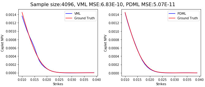
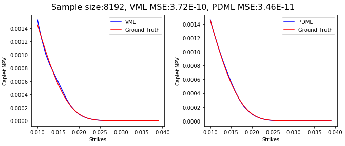
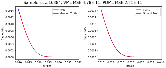
In Figure 6, we can see that PDML prices caplets more accurately than VML for a given sample size. In terms of sample efficiency, VML took $\sim 16K$ samples to achieve comparable accuracy obtained by PDML with $\sim 4K$ samples, thus PDML is about four times more sample efficient than VML.

Figure 7: Comparison of Derivative of Caplet Price wrt Strike from VML vs PDML Across Various Sample Sizes

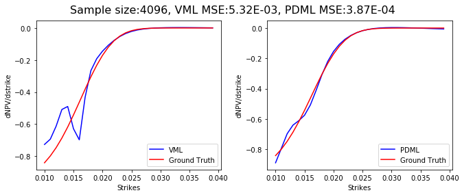
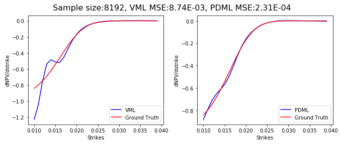
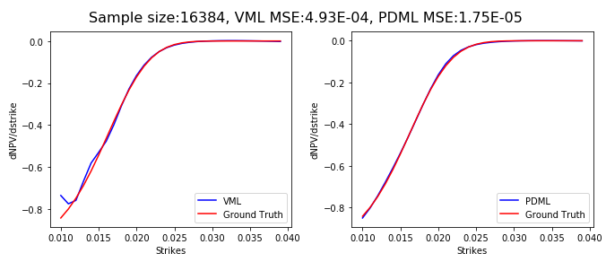
In Figure 7, we can see that for a given sample size, PDML predict derivatives with respect to strike better than VML. Furthermore, if the sample size is increased, the derivative with respect to strike as computed by PDML approximates the ground truth very closely whereas VML only approximates the price well but not the derivative with respect to strike. This can be seen from Figure 8 which uses large MC sample size $\sim 250K$. Both VML and PDML produce caplet prices close to ground truth. For the derivative with respect to strike, PDML gives values close to ground truth while the VML results differ appreciably from the ground truth for small caplet strikes.

Figure 8: Prediction of Price and Derivative by VML and DML with Large Sample Sizes

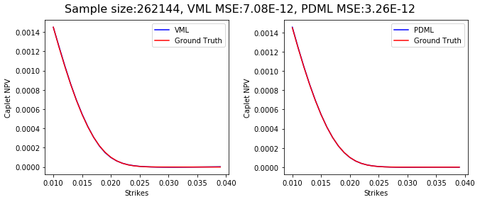
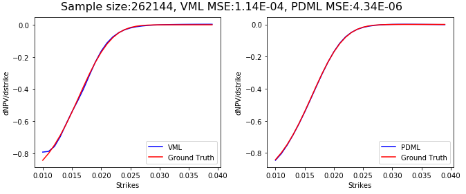
Thus, from the numerical results observed in this setting, we can conclude that regularizing the training with differentials with respect to the varied contract parameter yield faster convergence to ground truth for both the price and the derivative of the price with respect to the contract parameter.

Setting 2: In this setting, we consider varying model parameters and we fix the contract parameter (caplet strike) to ATM. We are using time-constant model parameters $a(t)\equiv a,b(t)\equiv b,\eta(t)\equiv 0.54224$. We generate varying model parameters $X_{i}=(a,b)\sim U(-0.15,-0.18)\times U(0.0065,0.0085)$. We use $2^{16}$ MC samples to train PDML & VML networks and compare caplet prices and derivatives of them with respect to model parameters computed with those networks against ground truth prices and derivatives computed with $10M$ MC samples for each parameter set.

Figure 9: Comparison of PDML vs VML for Prices and for Risk Sensitivities wrt Model Parameters

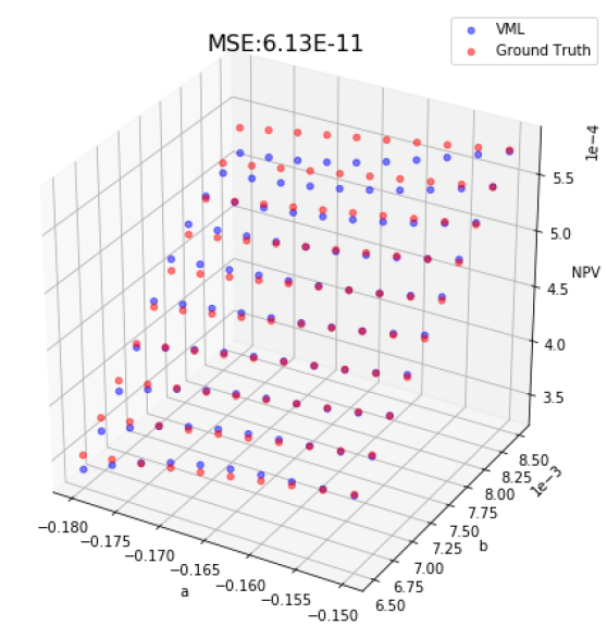
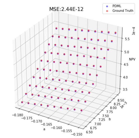
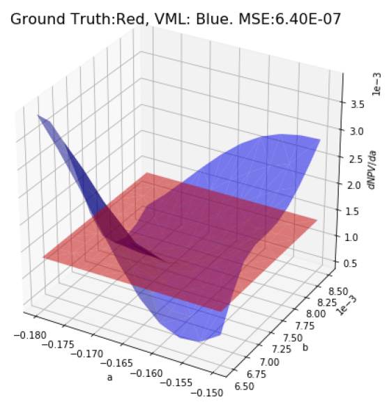
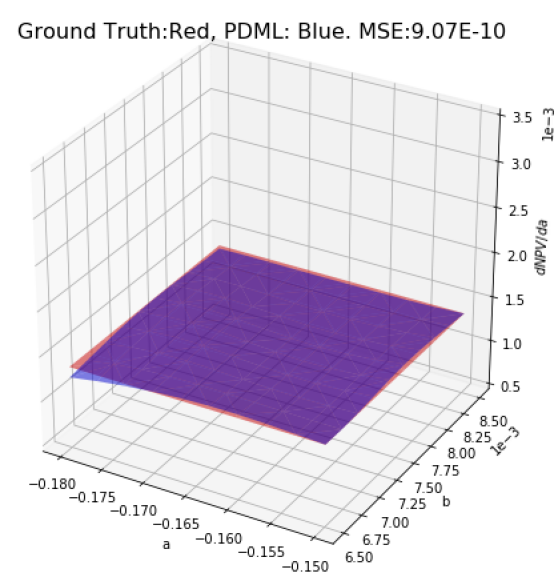
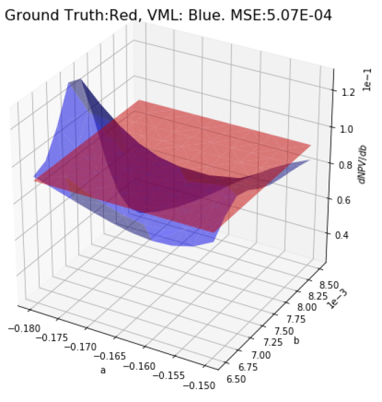
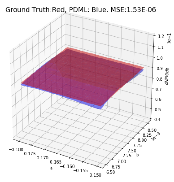
In Figure 9, we can see that PDML network is more accurate than VML network in computing caplet derivative price. We also see that VML network approximates risk sensitivities $\left(\frac{dNPV}{da},\frac{dNPV}{db}\right)$ very poorly while PDML network approximates the risk sensitivities quite well for this given sample size.

5.5 Pricing Results - Adaptive Parameter Sampling

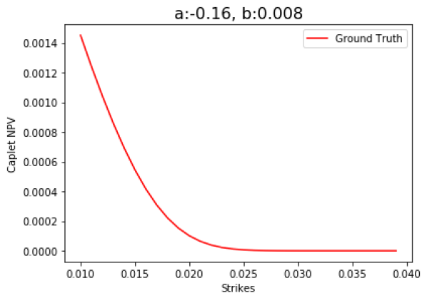
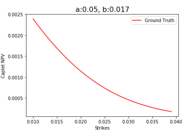
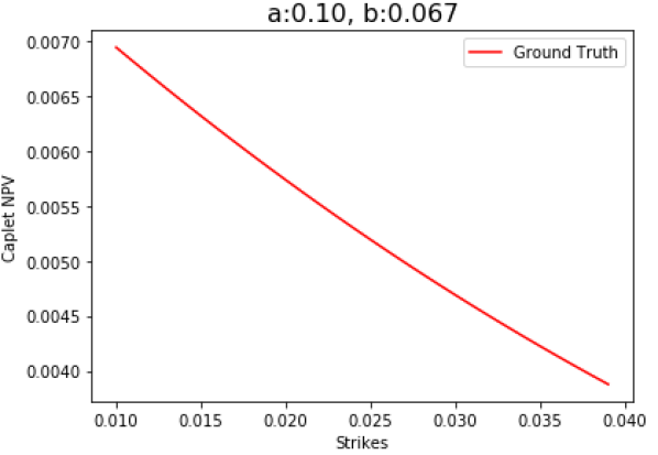
In Figure 10, we show that different model parameter values (here three example parameter sets on model parameter space $\left(a(t),b(t)\right)\equiv\left(a,b\right)\equiv[-0.16,0.1]\times[0.008,0.067]$) lead to conditional expectations (caplet prices) of different magnitude across strike range $[0.01,0.04]$, in particular for different $b$.

In calibration and other parametric pricing settings, it is important to achieve a certain relative accuracy for model parameters across the parameter range.

Figure 10: Ground Truth Prices for Different Parameter Sets Viewed Across Strikes. MC Prices with 10M Simulations are Considered as Ground Truth Prices.

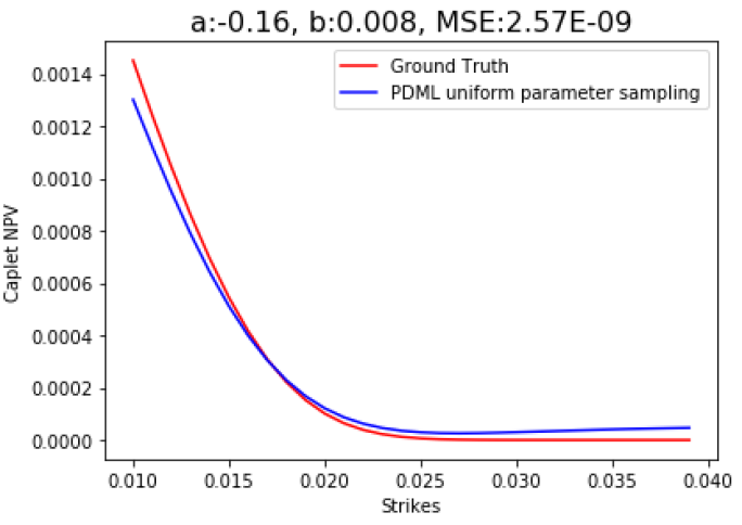
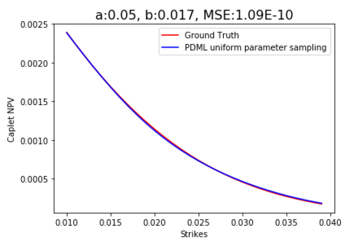
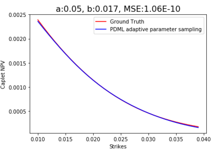
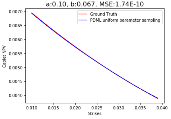
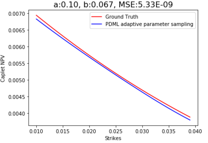
In Figure 11, we compare PDML network trained under uniform parameter sampling ( $X=(a,b,k)\sim U[-0.16,0.1]\times U[0.008,0.067]\times U[0.01,0.04]$) on the left with a PDML network trained under adaptive parameter sampling ( $X=(a,b,k)\sim U[-0.16,0.1]\times P[0.008,0.067]\times U[0.01,0.04]$) on the right. We can see on the left that for the top parameter set which results in conditional expectations smaller in magnitude, the PDML surrogate network does not approximate the ground truth well, while it does so in the lower two parameter sets for which the conditional expectations is larger in magnitude.

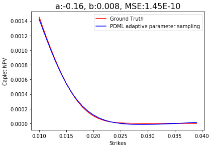
We can see on the right that using an adaptive sampling $P[0.008,0.067]$ for the $b$ parameter leads to better approximation for the top two parameter sets and to a slightly worse approximation which mostly preserves shape.

The adaptive sampling distribution P for parameter b is such that $P(b)\propto\frac{1}{E\left[.|b\right]}$. These marginal expectations $E\left[.|b\right]$ can be approximated by binning the samples by the $b$ parameter and computing bin averages. Using these averages, we compute a cubic spline fit to get a smooth approximation of $\frac{1}{E\left[.|b\right]}$. Finally, we scale the cubic spline fit appropriately so that it integrates to one and can be used as sampling distribution.

In this way, we sample parameter sets leading to smaller conditional expectations more often so that we will approximate those parameters regions better than with an uniform distribution. This will also lead to fewer samples in those parameter regions leading to larger conditional expectations, leading to some degradation of approximation quality there. If we want to approximate all regions as well as before, we will need to learn on a somewhat increased number of samples.

If we sample parameter ranges adaptively, MSE in regions with smaller magnitude of conditional expectation will decrease and in regions with higher magnitude of conditional expectation, MSE will increase. But, in a relative sense, adaptive parameter sampling provides better results than uniform sampling distribution, as $\left(MSE_{adaptive}/MSE_{uniform}\right)$ increases by a factor of about 10 in the lower magnitude region while it decreases by only $1/2$ in higher magnitude region.

Figure 11: Comparison of PDML Approximation Accuracy with Uniform vs Adaptive Parameter Sampling. Both PDML Surrogates Were Trained on MC Sample Sizes of $2^{16}$.

6 Calibration Based on Parametric Pricing DNN Surrogates

Calibration is a very important step in many quantitative finance applications and a key step in pricing and risk management of vanilla and exotic options. In calibration, one tries to find a set of model parameters that fits the market data for calibration instruments best in a certain way. There might be additional constraints and regularizations beyond best fit to calibration instrument market data. Typically what is considered best is expressed as an objective function parametrized over model parameters that compares pricing under the model with given model parameters against prices given by market data. Least squares or weighted least squares is a common form of objective function.

6.1 Calibration by Optimization

Calibration by optimization tries to find parameter sets that minimize that given objective function with appropriate optimization methods starting from appropriate initial guessses. Objective functions might have several local minima (which would be found by local optimization methods) and often one tries to find the global minimum or a good enough local minimum, thus favoring global or globalized optimizers. Typical calibration processes by optimization require calibration instruments repriced for each term in the objective function. The calibration through optimization is typically run until some stopping criterion is satisfied which could be a certain level of objective function to achieve, a certain maximum number of optimization steps or generations to perform, or to stop once the parameters change less than a certain amount as measured in some metric or the objective function changes less than a certain number over the last step and/or generation, or a combination of such criteria. We assume that the optimization method identifies and returns one parameter set as the “best” result, and we will call that parameter set the optimized parameter set.

The standard approach generally involves the development of analytical or semi-analytical pricers for a simplified model and/or analytical or semi-analytical approximative pricers for the original problem. This means a major theoretical and implementation effort to first identify appropriate simplifications, approximations, and assumptions and then implement both the simplification and approximation process and the (approximate) pricer for the (approximate) problem. These simplifications, approximations, and assumptions often introduce errors and biases so that close-to-optimal parameter sets for the approximate set-up are no longer close-to-optimal for the original model.

Alternatively, one could use a possibly parallelized MC pricer for the vanilla calibration instruments insider of the global optimizer (such as differential evolution - DE). While this avoids the need of deriving approximations and simplifications and implementing special solvers, it is typically very compute intensive and the number of MC paths or samples used in the pricer has to be kept small so that the calibration process can be run with the available computing power. Often, this requires finding and implementing sufficiently good control variates or other variance reduction techniques, forcing the derivation and implementation of good enough control variates or the introduction of uncontrollable and unmonitored bias and/or variance due to the use of approximate MC sampling on a small number of paths.

We propose the use of PDML techniques to obtain one or several DNN surrogates for the pricing function derived from differentiable simulation of the underlying model with apppropriately sampled parameters, to optimize with global optimizers (and potentially to refine with local optimizers) over these surrogates, and to return a parameter set that performs well enough in a ground truth or reference pricer.

If calibrating to calibration instruments of different maturities, one can either proceed with a time-global calibration—where model parameters across all time intervals are calibrated at the same time, allowing time-homogenous models or models with almost any kind of term structure—or a piecewise calibration, where constant model parameters are determined for each time interval between maturities. Often piecewise calibration (“bootstrapping”) is preferred. For multiple maturities, we will discuss and use piecewise calibration.

Thus, the calibration approaches that we will be using are the following:

Calibration Approach: Single Maturity. To calibrate the model parameters from given caplet prices for maturity $T$, we assume the model parameters $\Theta_{S}$ are constant over the time period $[0,T]$, i.e., $a(t)\equiv a,b(t)\equiv b,$ and $\eta(t)\equiv\eta$ for the Cheyette model. Next, we set the interval bounds for input space and generate the training data set $\left\{X_{i},Y_{i}\right\}_{i=1}^{m}$ respectively $\left\{X_{i},Y_{i},DY_{i}\right\}_{i=1}^{m}$ where $X_{i}=\left(a^{i},b^{i},\eta^{i},k^{i}\right)$ is sampled using adaptive parameter sampling, with model parameters $\Theta^{i}_{S}=\left(a^{i},b^{i},\eta^{i}\right)$ and contract parameters $\Theta^{i}_{F}=\left(k^{i}\right)$. The output $Y_{i}$ is obtained as one MC sample and here it denotes the pathwise payoff of the caplet with strike price $k^{i}$, maturity $T$, and appropriate tenor (0.25/3M with the appropriate daycount). The output $DY_{i}$ (full set of derivatives of $Y_{i}$ with respect to the model parameters and the contract parameter (strike)) can be obtained by algorithmic differentiation from the computational graph for the MC sampling and is computed in TensorFlow as needed.

We use PDML technique with this training data to learn a surrogate $\hat{f}\left(X\right)\approx E\left[Y|X\right]$ where $Y$ is the caplet payoff. Then, finally we use $\hat{f}$ inside a (global) optimization method (such as ICDE) where different calibration contracts correspond to varying $\Theta_{F}$ and find the optimized model parameters $\Theta_{S}$ under calibration (here, for the Cheyette model, $\Theta_{S}=\left(\underline{a},\underline{b},\underline{\eta}\right)$.

Calibration Approach: Multiple Maturities. We perform piecewise-time constant model parameter calibration based on given caplet prices and/or caplet volatility surface of different maturities and appropriate 3M tenor. Organize the maturities $\left\{T_{i}\right\}_{i=1}^{N}$ so that $0=T_{0}<T_{1}<\dots<T_{N}$. We assume $a(t)\equiv a_{i},b(t)\equiv b_{i},$ and $\eta(t)\equiv\eta_{i}$ for $t\in[T_{i-1},T_{i})$, $i=1,\dots,N$ for this Cheyette model calibration or $\Theta_{S}(t)\equiv\Theta_{S,i}$ in the general case. The calibration procedure is as follows: First, we calibrate the model parameters of the left most time interval $[0,T_{1})$ as described in the calibration approach for single maturity and obtain optimized parameters $\underline{\Theta}_{S,1}=\underline{a}_{1},\underline{b}_{1},\underline{\eta}_{1}$. We then fix these model parameters $\underline{\Theta}_{S,1}=\underline{a}_{1},\underline{b}_{1},\underline{\eta}_{1}$ for time interval $[0,T_{1})$ and repeat for the next consecutive time interval $[T_{1},T_{2})$ to obtain optimized parameters $\underline{\Theta}_{S,2}=\underline{a}_{2},\underline{b}_{2},\underline{\eta}_{2}$. We repeat until we calibrate the model parameters of right most interval $[T_{N-1},T_{N}]$ and obtain $\underline{\Theta}_{S,N}=\underline{a}_{N},\underline{b}_{N},\underline{\eta}_{N}$.

6.2 Global Optimization Methods

To perform the optimization for the calibration, appropriate optimization methods are needed. We will at first use generic global or globalized optimization methods that can reliably handle optimization problems of various kinds, even though any particular optimization problem that we apply it to might be such that simpler or more specialized optimization methods might work. Even though PDML provides parameter derivatives, the chosen optimization method might not take (full) advantage of it. While PDML surrogates are in general at least as accurate as VML and more accurate than MC pricers with small number of paths, they might be of limited and not specified accuracy, and thus trying to solve the optimization problems more accurately than the surrogates are might not be advisable. At least some of the models typically calibrated in quantitative finance (such as Heston) are known to have involved topology and geometry and allow several local minima, thus we are lead to consider global or globalized optimization methods.

There are many global and globalized optimizers described in the literature. To name a few: for global approches, there are a variety of differential evolution (DE) variants and particle swarm optimization (PSO) variants, simulated annealing (SA), and other genetic algorithms (GA) or evolutionary algorithms (EA). Globalized approaches include the usual local optimization methods such as Gauss-Newton, Newton-Raphson, L-BFGS etc. but started from random or otherwise widely sampled parameter sets. One can also start these local methods with populations or sets of parameter intervals determined by some first stage algorithm.

We had previously implemented an improved constrained differential evolution (ICDE) global optimization routine in Python and in C++ [JWCJ13] which performs well and can be easily parallelized while also being able to handle equality and inequality constraints. Besides the equality and inequality constraints, one is also given a (hyper-)rectangular search space defined by intervals for each component of the parameter vector under minimization. ICDE is a further developed variant of differential evolution [PSL05]. Differential evolution is a simple yet efficient evolutionary algorithm starting from some initial population that is typically randomly sampled from the given intervals; and then undergoes crossover, mutation, selection, enforcement of boundary constraints etc. to produce a number of generations. ICDE [JWCJ13] uses crossover strategies rand/1, rand/2, current to rand/1, and current to best/1 and improved breeder genetic algorithm (IBGA). Constraints are treated by minimizing the degree of constraint violation as defined appropriately. All the parameter sets to be evaluated for the next generation are collected and then evaluated in parallel with several backends to allow parallel processing through Python’s multiprocessing or joblib facilities or similar.

In our tests, this ICDE implementation performed well enough. In future work, we intend to test other global and/or globalized optimization methods that potentially could take advantage of derivative information, and possibly lead to faster and/or more robust methods.

6.3 Impact of Randomness on Surrogates: Making Optimization More Robust

When calibrating with surrogates obtained by PDML, we are using random numbers at several points during the process. First, we consume random numbers during the parameter and MC sampling to generate $X$, $Y$, and $DY$. Then, the DNN for PDML are initialized according to some random initializations (in our DNN architecture, these would be the weights and biases).

Then, the DNN in the PDML step are trained by stochastic gradient descent methods with Adam Momentum, which might consume additional random numbers. Once the surrogates have been constructed, the global optimization method (such as ICDE) might also consume random numbers (in fact, ICDE uses random numbers to construct a new population of parameter sets from the old one). All these random numbers could be generated from either a single stream or from several streams with their own seed(s). Different choice of such seeds will in general lead to variation in results and thus training several surrogates in parallel and optimizing against them will lead in general to different surrogates and different optimized parameter sets. These parameter sets associated to different seeds might correspond to differently accurate DNN networks that lead to optimized parameter sets of different accuracies.

Running independent constructions of PDML surrogates and optimizing over them starting with different seeds on different instances is perfectly parallel. Given the multi-core nature of common commodity CPU, one can obtain 5-10 replications at essentially the same running time as one replication; and on elastic compute units or larger server farms, this scales to even higher number of replications.

Once we have constructed several replications in parallel in this way, we quantify the variation in the results of those replications through two metrics: ‘PDML fit error’ and ‘Model error’ as follows:

PDML fit error $$= \sum_{\text{instruments}}\left(\text{PDMLapproximation}-\text{MC estimate}\right)^{2}$$ (50)

Model error $$= \sum_{\text{instruments}}\left(\text{MC estimate}-\text{target price}\right)^{2}$$ (51)

Here, PDMLapproximation stands for the pricing with the PDML surrogate in that replication with the optimized parameter set from that replication, MC estimate stands for the MC pricing with the optimized parameter set from that replication with enough samples (to estimate ground truth), and target price stands for the price of the calibration instruments as provided by market data or market data objects (such as caplet volatility surfaces together with appropriate Black or Bachelier formulas).

For the $i^{th}$ step in the multi-maturity calibration procedure, these metrics can be re-written as follows:

PDML fit error $$= \sum_{\Theta_{F}}\left(\hat{f}\left(\underline{\Theta}_{S,i},\Theta_{F}\right)-MC\left(\underline{\Theta}_{S,i},\Theta_{F}\right)\right)^{2}$$ (52)

Model error $$= \sum_{\Theta_{F}}\left(MC\left(\underline{\Theta}_{S,i},\Theta_{F}\right)-MKT(\Theta_{F})\right)^{2}$$ (53)

where $\Theta_{F}=(k)$ denotes the contract parameter(s) (caplet strike in our example), $MC(.)$ denotes the MC price obtained by enough samples (to estimate ground truth) with $\underline{\Theta}_{S,i}=\left(\underline{a}_{i},\underline{b}_{i},\underline{\eta}_{i}\right)$ as model parameters and $MKT(\Theta_{F})$ denotes the market or target price.

Based on these metrics, we can select a best seed or set of best seeds to define some robustification to the optimization. That robustification will have results less dependent on any particular seed and likely perform better than an optimization run with only one particular seed. We propose two robust calibration approaches, namely, best seed approach and ensemble approach.

The best seed approach is as follows:

1. Set seed for NN weight initialization, optimization algorithm, MC sample generation and run calibration. Repeat the process with several seeds.

2. Select the best seed based on two metrics as follows:

   $$\text{bestseed}=\min_{\text{seed}}\max\left(\text{PDML fit error},\text{Model error}\right)$$ (54)

3. The optimal model parameters corresponding to the best seed are selected.

The ensemble approach is as follows:

1. Set seed for NN weight initialization, optimization algorithm, MC sample generation and run calibration. Repeat the process with several seeds.

2. Pick a set of seeds with least $\max\left(\text{PDML fit error},\text{Model error}\right)$.

3. Use the PDML networks corresponding to the selected seeds from the previous step to form an ensemble network. This ensemble network can be formed by averaging the results from individual component networks.

4. Finally, run the calibration part again but use the ensemble network as surrogate and obtained optimized parameters.

We have observed that the seed for the global optimization in the calibration has a relatively small impact on the results and thus we pick the seed corresponding to the best replication in the final calibration against the ensemble.

7 Calibration Setting and Results

7.1 Calibration Setting

We calibrate Cheyette models from caplet prices for maturities from 1 year to 6 years, all for tenor 3M, with the PDML technique. We show calibrations to single maturity data and settings and multi-maturity data and settings. We demonstrate both single-seed as well as robustified optimizations.

As is common when calibrating Cheyette models and other similar interest rate models, mean reversion speed $\kappa$ for the Cheyette SDEs and ODEs and mean reversion speed $\theta$ for the stochastic volatility process are chosen according to other considerations and instruments before calibrating to caplets or swaptions (see [AP10] for a discussion). In this calibration section, we fix them to the values $\kappa=0.03$ and $\theta=0.2$ for our numerical tests.

7.2 Single Seed Calibration Approach: Single Maturity

In single seed calibration approach, we use one single seed for NN weight initialization, DE optimization algorithm, and MC sample generation. In this section, we report numerical results when we calibrate models with constant model parameters against single-maturity data corresponding to different maturities. In particular, we work with six yearly maturities starting from 1 year to 6 years. We repeat the calibration with two different seeds.

Figure 12: Single Seed Calibration Approach: Single Maturity. Prices From PDML Network Trained Using Seed:2476 and MC for Optimized Parameter Sets Compared to Market Prices. (a) 1yr Maturity (b) 2yr Maturity (c) 3yr Maturity (d) 4yr Maturity (e) 5yr Maturity (f) 6yr Maturity.

Figure 13: Single Seed Calibration Approach: Single Maturity. Prices From PDML Network Trained Using Seed:5670 and MC at Optimized Parameter Sets Compared to Market Prices. (a) 1yr Maturity (b) 2yr Maturity (c) 3yr Maturity (d) 4yr Maturity (e) 5yr Maturity (f) 6yr Maturity.

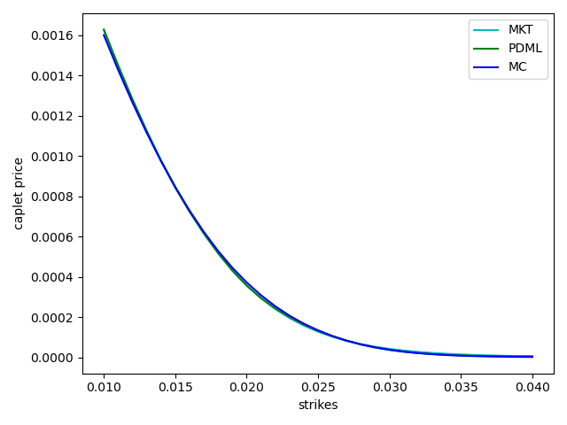
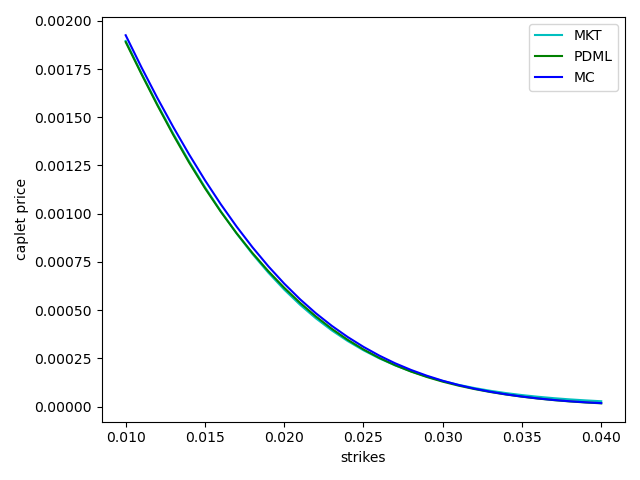
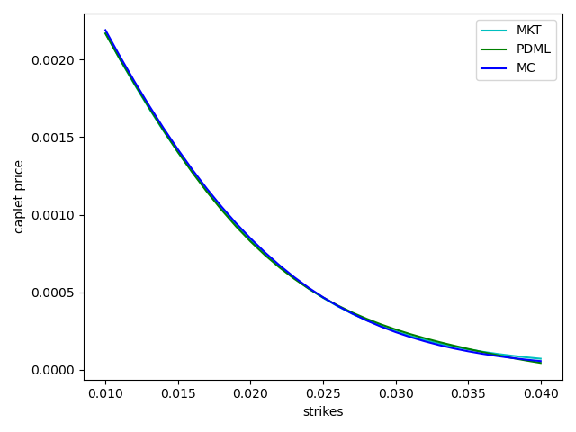
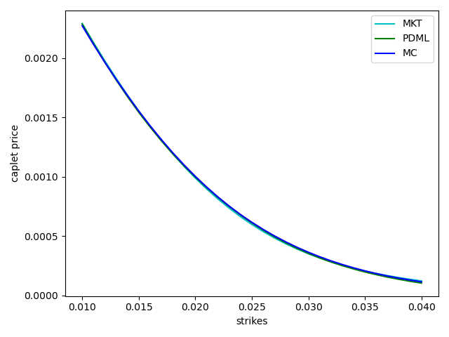
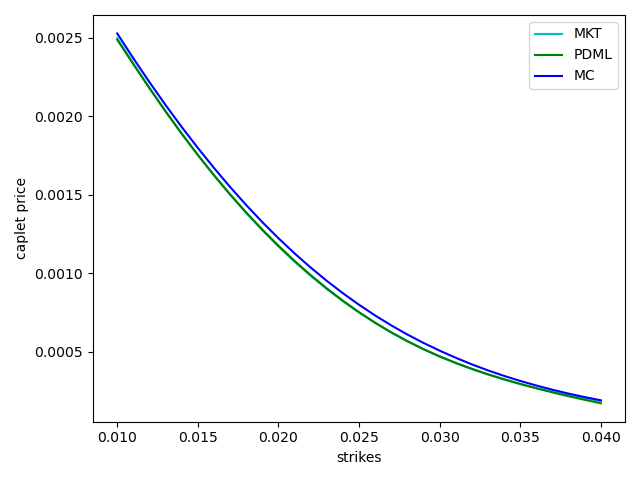
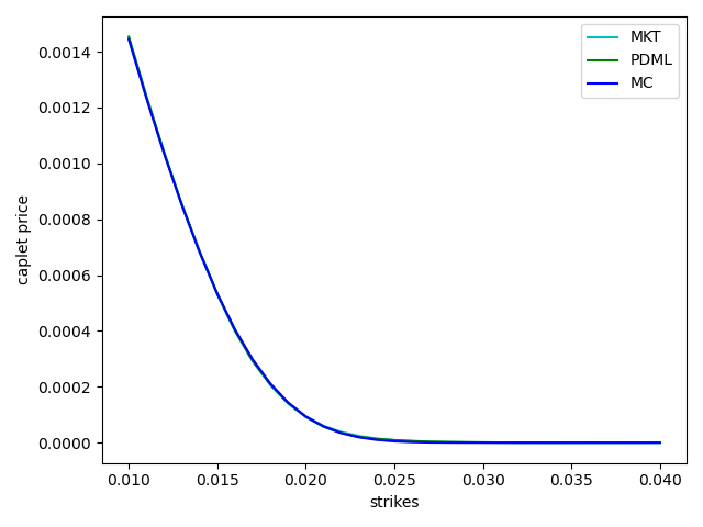
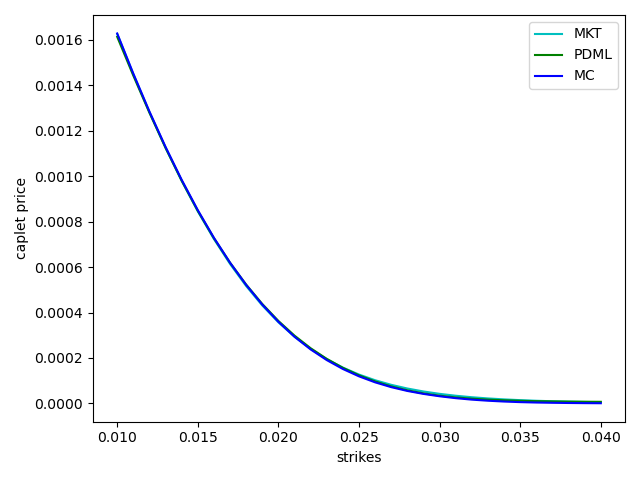
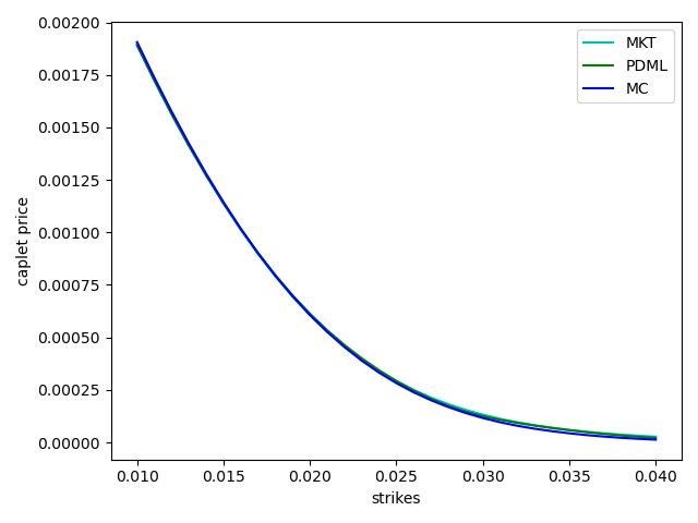
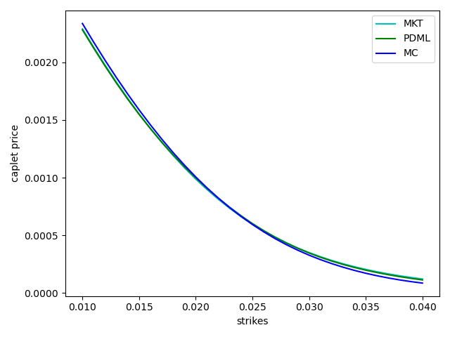
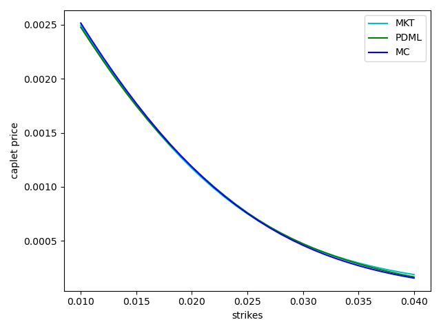
Figures 12 and 13 depict the results corresponding to the two different seeds. In both figures, results are reasonably accurate except 3 year and 6 year maturities in Figure 12 and except 4 year and 5 year maturities in Figure 12. Thus, using any single seed may or may not yield optimized parameter sets with reasonable accuracy for all maturities. Therefore, we are interested in more robust calibration approaches that are less sensitive to particular seeds and give accurate enough results for tests at all maturities.

7.3 Single Seed Calibration Approach: Multiple Maturities

In Table 1, we consider five different set of seeds and for each seed we report the two metrics when calibrating against multiple maturities. We can see that using one single seed may or may not lead to uniformly good or comparable accuracy for all maturities. If by chance that single seed is “bad” for some or most maturities, results will be less accurate and calibration will be less reliable.

Maturity	Metric	Seed:2476	Seed:4548	Seed:5670	Seed:5818	Seed:8642
1 yr	PDML fit error	9.13E-11	6.49E-12	8.71E-12	1.11E-11	2.40E-12
	Model error	8.90E-11	9.53E-12	1.42E-11	1.92E-11	9.62E-12
2 yr	PDML fit error	5.14E-10	3.18E-11	2.34E-11	8.62E-11	2.20E-11
	Model error	5.17E-10	2.91E-11	4.62E-11	1.15E-10	3.43E-11
3 yr	PDML fit error	3.03E-10	1.92E-11	1.65E-11	2.49E-10	8.98E-12
	Model error	2.96E-10	3.32E-11	6.52E-11	2.83E-10	1.81E-11
4 yr	PDML fit error	1.02E-09	5.83E-11	3.47E-11	2.78E-11	8.54E-11
	Model error	1.02E-09	7.02E-11	1.14E-10	1.10E-10	8.65E-11
5 yr	PDML fit error	1.24E-09	1.76E-10	9.42E-11	2.48E-10	8.97E-11
	Model error	1.23E-09	2.12E-10	2.09E-10	3.33E-10	8.21E-11
6 yr	PDML fit error	1.61E-09	1.46E-10	1.34E-10	3.87E-10	5.62E-11
	Model error	1.62E-09	1.99E-10	3.03E-10	5.00E-10	8.17E-11

Table 1: Single Seed Calibration Approach: Multiple Maturities. Calibration Results for Multiple Maturities Calibrations for Five Different Seeds.

7.4 More Robust Calibration Approach: Single Maturity

In this section, we test the more robust calibration approaches that we proposed for the single maturity case. In both of these robust calibration approaches, we run the calibration with five different seeds. For the best seed approach, we pick the best seed. For the ensemble, we form an ensemble network based on the best three seeds.

Figure 14: More Robust Calibration Approach: Single Maturity. Prices From Best Seed PDML Network and MC at Optimized Parameter Sets Compared to Market Prices. (a) 1yr Maturity (b) 2yr Maturity (c) 3yr Maturity (d) 4yr Maturity (e) 5yr Maturity (f) 6yr Maturity.

Figure 15: More Robust Calibration Approach: Single Maturity. Prices From Ensemble PDML Network and MC at Optimized Parameter Sets Compared to Market Prices. (a) 1yr Maturity (b) 2yr Maturity (c) 3yr Maturity (d) 4yr Maturity (e) 5yr Maturity (f) 6yr Maturity.

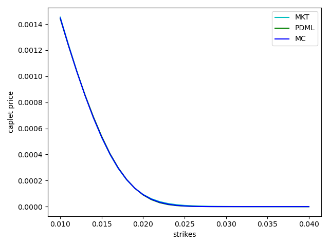
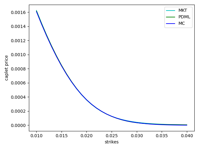
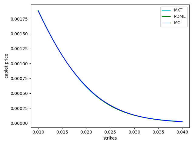
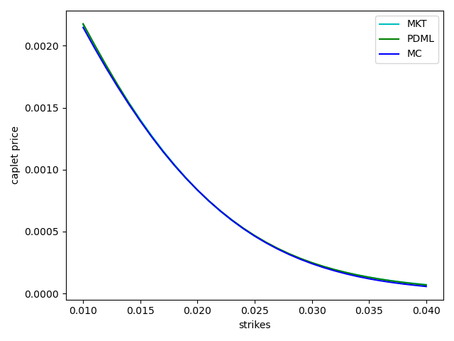
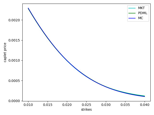
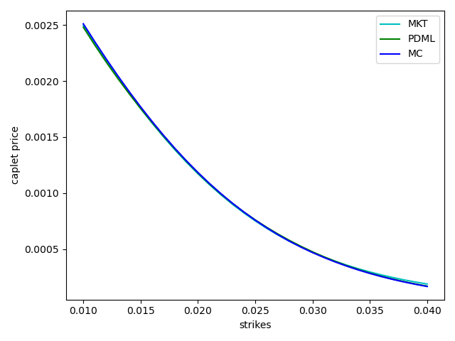
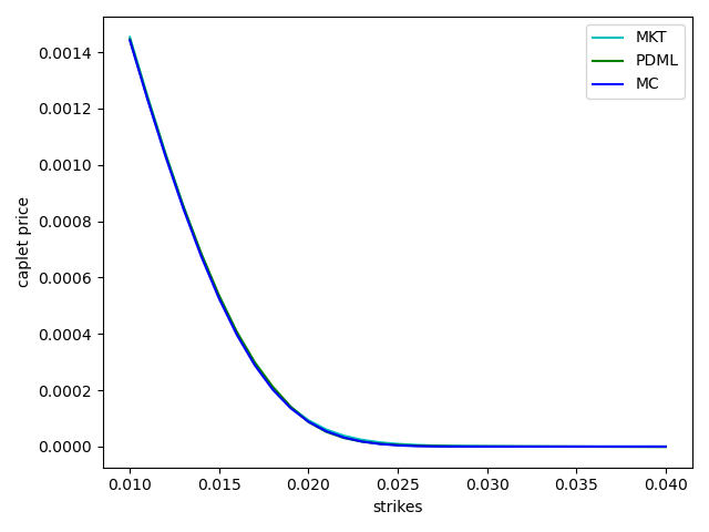
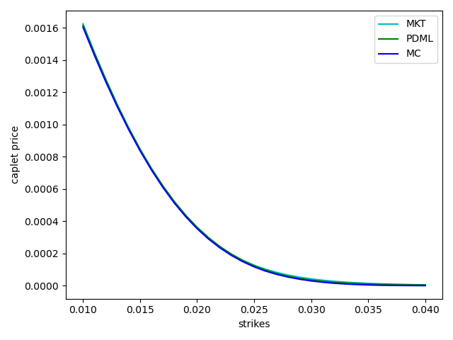
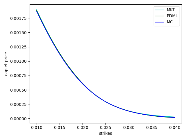
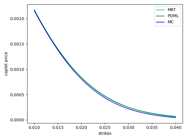
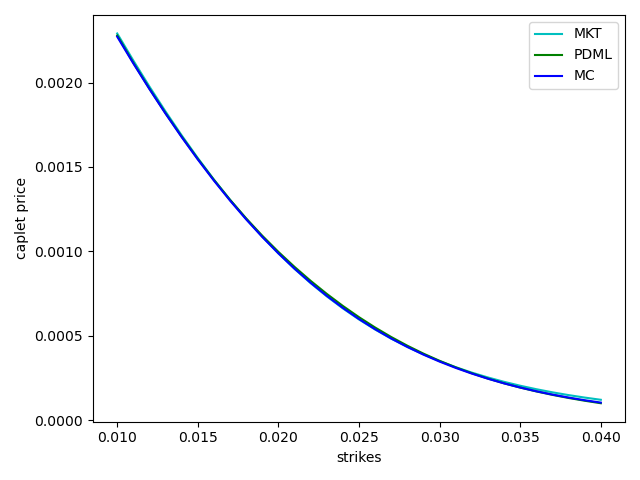
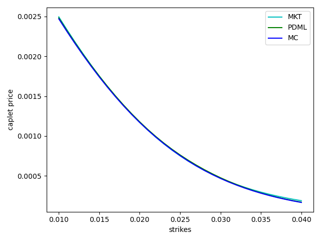
In Figure 14, we see that the best seed calibration approach yielded sufficiently accurate results for all the maturities considered. In Figure 15, we present the results corresponding to an ensemble PDML network corresponding to an ensemble made from the PDML networks corresponding to the best three seeds. Except for 4 year maturity, all maturities are calibrated sufficiently accurate with the ensemble approach also. In further testing, we observed that for the 4 year maturity case, the best two seeds produced quite accurate networks while the third best performed quite a bit worse in terms of metrics and affected the quality of the ensemble network. One could either consider some adaptive selection of seeds or form ensembles starting from more seeds and selecting the best three seeds from those (say, ensemble best 2 out of 5 or best 3 out of 8). In this particular case, a best 2 out of 5 ensemble would have given sufficiently accurate results for all maturities.

7.5 More Robust Calibration Approach: Multiple Maturities

In Table 2, we report results from the best seed approach. The best seed is chosen such that it has least max error (highlighted in bold). We can see that the best seed approach resulted in lower PDML fit error and Model error across all maturities.

Maturity	Metric	Seed:2476	Seed:4548	Seed:5670	Seed:5818	Seed:8642
1 yr	PDML fit error	9.13E-11	6.49E-12	8.71E-12	1.11E-11	2.40E-12
	Model error	8.90E-11	9.53E-12	1.42E-11	1.92E-11	9.62E-12
	max error	9.13E-11	9.53E-12	1.42E-11	1.92E-11	9.62E-12
2 yr	PDML fit error	1.81E-10	2.30E-11	1.17E-11	8.40E-12	8.77E-11
	Model error	1.84E-10	3.17E-11	2.47E-11	2.78E-11	9.73E-11
	max error	1.84E-10	3.17E-11	2.47E-11	2.78E-11	9.73E-11
3 yr	PDML fit error	9.69E-10	1.82E-11	1.26E-10	2.44E-11	6.72E-11
	Model error	9.73E-10	2.80E-11	1.27E-10	2.38E-11	8.92E-11
	max error	9.73E-10	2.80E-11	1.27E-10	2.44E-11	8.92E-11
4 yr	PDML fit error	1.44E-10	2.01E-11	2.39E-10	4.40E-11	3.24E-10
	Model error	1.21E-10	3.79E-11	2.62E-10	6.00E-11	3.16E-10
	max error	1.44E-10	3.79E-11	2.62E-10	6.00E-11	3.24E-10
5 yr	PDML fit error	1.02E-09	3.46E-12	6.20E-11	3.22E-11	2.35E-10
	Model error	1.02E-09	4.09E-11	6.20E-11	6.37E-11	2.25E-10
	max error	1.02E-09	4.09E-11	6.20E-11	6.37E-11	2.35E-10
6 yr	PDML fit error	2.14E-09	1.35E-10	2.27E-10	4.32E-11	1.26E-10
	Model error	2.12E-09	1.90E-10	2.65E-10	1.09E-10	1.49E-10
	max error	2.14E-09	1.90E-10	2.65E-10	1.09E-10	1.49E-10

Table 2: More Robust Calibration Approach: Multiple Maturities. Calibration Results for Multiple Maturities From Best Seed Approach.

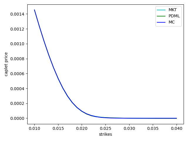
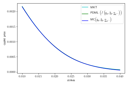
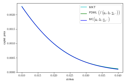
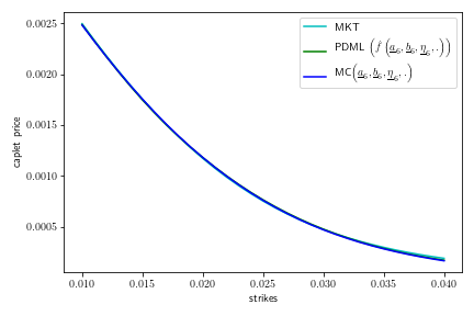
In Figure 16, we compare the price graphs of best seed PDML network and MC at optimized parameter sets $\left(\underline{a}_{i},\underline{b}_{i},\underline{\eta}_{i}\right)$ against market prices across a range of strikes for $i=1,\dots,6$. We can see that the optimized parameter sets from the best seed calibration approach reproduced market prices very well across range of strikes for all maturities considered.

Figure 16: More Robust Calibration Approach: Multiple Maturities. Prices From Best Seed PDML Network and MC at Optimized Parameter Sets Compared to Market Prices. (a) 1yr Maturity (b) 2yr Maturity (c) 3yr Maturity (d) 4yr Maturity (e) 5yr Maturity (f) 6yr Maturity.

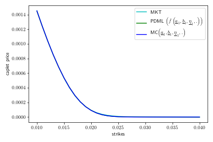
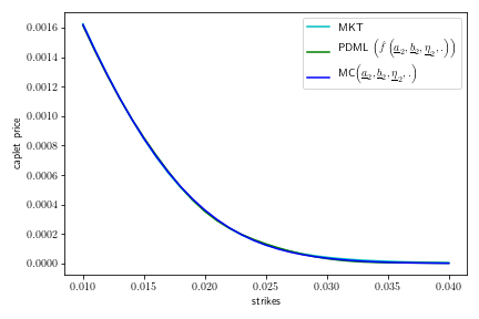
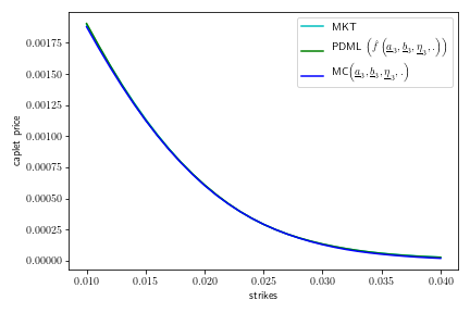
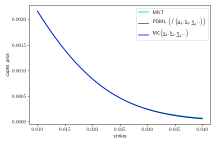
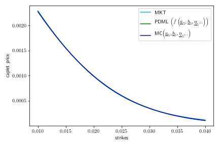
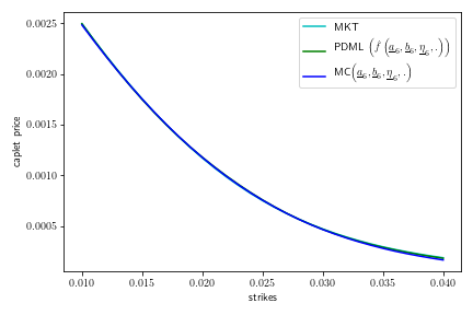
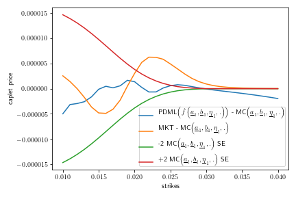
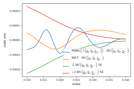
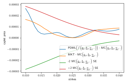
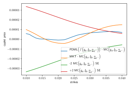
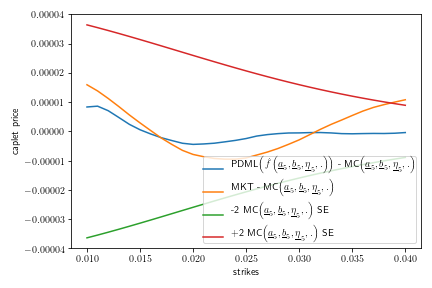
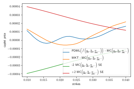
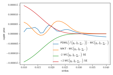
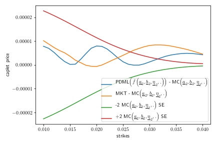
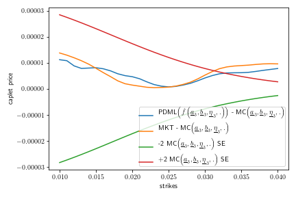
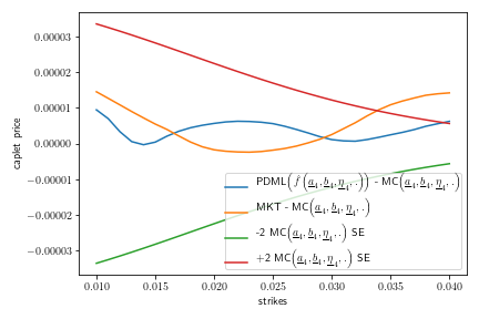
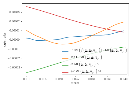
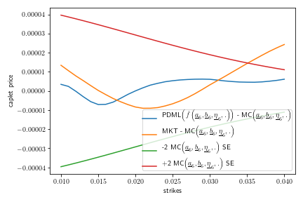
In Figure 17, we analyze prices more closely by looking at differences with respect to approximate ground truth, here represented by MC with enough samples. PDML$\left(\hat{f}\left(\underline{a}_{i},\underline{b}_{i},\underline{\eta}_{i},.\right)\right)$ - MC$\left(\underline{a}_{i},\underline{b}_{i},\underline{\eta}_{i},.\right)$ shows how well the PDML network replicated MC at the optimized parameter set $\left(\underline{a}_{i},\underline{b}_{i},\underline{\eta}_{i}\right)$. MKT - MC$\left(\underline{a}_{i},\underline{b}_{i},\underline{\eta}_{i},.\right)$ shows how well the optimized parameter set approximates calibration target prices (MKT) by considering MC with enough samples as approximate ground truth. $\pm 2$MC$\left(\underline{a}_{i},\underline{b}_{i},\underline{\eta}_{i},.\right)$ SE standard error bars are provided as base line to assist in comparing differences. Except for 1 year maturity, the differences are well within 2 standard error bars for most of the strikes, indicating that optimized parameter sets reproduced market prices very well and that the best seed PDML network agrees well with MC approximation of ground truth at those parameter sets.

For the 1 year maturity, the PDML network is close to MC with enough samples and thus ground truth. Both are somewhat away from the target prices within the middle and right of the strike range. To be able to reprice those target prices in that region very well, one cannot assume that the model parameters are constant across the first year; one would need to calibrate to shorter maturities also, say 3M, 6M, and 9M, and calibrate model parameters for each quarter, or one would need to introduce a different and richer parametrization for the volatility term rather than the linear one used here. Thus, this corresponds to a model parametrization limitation rather than a limitation of the calibration and would be seen regardless of calibration method.

Figure 17: More Robust Calibration Approach: Multiple Maturities. Comparing Price Differences: Best Seed PDML Network Prices vs MC Prices and vs Market Prices for Optimized Parameter Sets. (a) 1yr Maturity (b) 2yr Maturity (c) 3yr Maturity (d) 4yr Maturity (e) 5yr Maturity (f) 6yr Maturity.

In Table 3, we present calibration results from the ensemble calibration approach. The blue color highlights the least max error and the red color highlights the highest max error among the five different seeds. We can see that ensemble results are close to least max error (blue) and sometimes better, for instance for 2 year maturity (highlighted in bold).

Maturity	Metric	Seed:2476	Seed:4548	Seed:5670	Seed:5818	Seed:8642	Ensemble
1 yr	PDML fit error	9.13E-11	6.49E-12	8.71E-12	1.11E-11	2.40E-12	4.28E-12
	Model error	8.90E-11	9.53E-12	1.42E-11	1.92E-11	9.62E-12	1.07E-11
	max error	9.13E-11	9.53E-12	1.42E-11	1.92E-11	9.62E-12	1.07E-11
2 yr	PDML fit error	2.56E-10	6.09E-11	1.70E-10	9.40E-12	5.28E-11	1.44E-11
	Model error	2.35E-10	5.92E-11	1.80E-10	3.35E-11	5.77E-11	3.16E-11
	max error	2.56E-10	6.09E-11	1.80E-10	3.35E-11	5.77E-11	3.16E-11
3 yr	PDML fit error	2.94E-10	2.78E-11	9.89E-12	3.08E-11	6.48E-11	2.22E-11
	Model error	3.05E-10	6.07E-11	4.20E-11	6.48E-11	1.22E-10	5.17E-11
	max error	3.05E-10	6.07E-11	4.20E-11	6.48E-11	1.22E-10	5.17E-11
4 yr	PDML fit error	1.46E-09	4.97E-11	1.55E-10	2.00E-11	7.78E-12	1.50E-11
	Model error	1.52E-09	9.27E-11	2.02E-10	7.40E-11	6.09E-11	6.47E-11
	max error	1.52E-09	9.27E-11	2.02E-10	7.40E-11	6.09E-11	6.47E-11
5 yr	PDML fit error	3.30E-10	1.46E-10	2.50E-10	5.48E-11	3.86E-11	3.28E-11
	Model error	3.51E-10	1.94E-10	2.98E-10	8.17E-11	8.00E-11	8.45E-11
	max error	3.51E-10	1.94E-10	2.98E-10	8.17E-11	8.00E-11	8.45E-11
6 yr	PDML fit error	7.33E-10	1.17E-11	9.20E-11	3.07E-10	9.35E-10	3.88E-12
	Model error	7.73E-10	8.99E-11	1.77E-10	3.78E-10	1.02E-09	9.78E-11
	max error	7.73E-10	8.99E-11	1.77E-10	3.78E-10	1.02E-09	9.78E-11

Table 3: More Robust Calibration Approach: Multiple Maturities. Calibration Results With Ensemble Approach for Multiple Maturities.

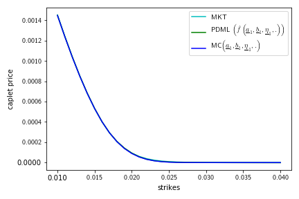
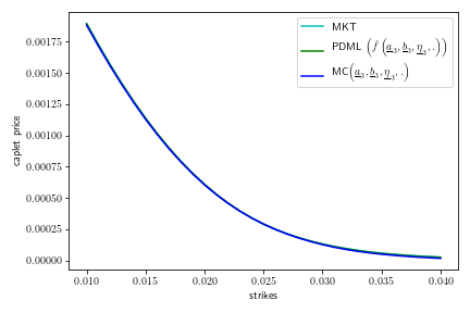
In Figures 18 and 19, we can see that ensemble approach has similar results as best seed approach in Figures 16 and 17. In Table 4, we can see that the accuracy of best seed and ensemble approaches is similar. As both approaches have similar accuracy, we chose the best seed approach for our calibration application as best seed approach has smaller computational cost than the ensemble approach. Nonetheless, we believe ensemble approach could be a good alternative approach for calibration with PDML technique, in particular also for other models and set-ups.

Figure 18: More Robust Calibration Approach: Multiple Maturities. Comparing Ensemble PDML Network Prices vs MC Prices and vs Market Prices for Optimized Parameter Sets. (a) 1yr Maturity (b) 2yr Maturity (c) 3yr Maturity (d) 4yr Maturity (e) 5yr Maturity (f) 6yr Maturity.

Figure 19: More Robust Calibration Approach: Multiple Maturities. Comparing Price Differences: Ensemble PDML Network Prices vs MC Prices and vs Market Prices for Optimized Parameter Sets. (a) 1yr Maturity (b) 2yr Maturity (c) 3yr Maturity (d) 4yr Maturity (e) 5yr Maturity (f) 6yr Maturity.

Maturity \Approach	Best seed	Ensemble
1yr	9.53E-12	1.07E-11
2yr	2.47E-11	3.16E-11
3yr	2.44E-11	5.17E-11
4yr	3.79E-11	6.47E-11
5yr	4.09E-11	8.45E-11
6yr	1.09E-10	9.78E-11

Table 4: More Robust Calibration Approach: Multiple Maturities. Comparison of Max Error of Best Seed and Ensemble Approaches.

8 Conclusion

In this paper, we demonstrated how Parametric Differential Machine Learning (PDML) can produce accurate enough parametric pricing surrogates for conditional expectations of functionals from samples of the functional and sample-wise derivatives of samples with respect to parameters for appopriately sampled parameters as generated by differentiable simulation and computation from text input close to mathematical notation. If different model parameters lead to prices of different magnitudes, adaptive parameter sampling is used to improve relative approximation for parameter ranges for which the magnitude of the price is smaller, leading to better approximation and calibration in such parameter ranges. These parametric pricing surrogates can stand in for specialized solvers for purposes such as calibration and speed up the calibration. Since the sampling, the construction of surrogates, and the optimization for calibration is impacted by randomness; one can generate different surrogates and different optimized parameter sets from different seeds. Once a ground truth indicator has been implemented, one can then pick surrogates that approximate ground truth well and approximate calibration target prices, at least close to the optimized parameter sets. Such surrogates and optimization methods will be more accurate and more reliable than what would be obtained with a single seed.

We demonstrated parametric pricing and calibration for interest rate caplets for Cheyette Models with benchmark rate volatility specification with an additional stochastic volatility factor and obtain good results.

As such, the demonstrated parametric differential machine learning approach to parameteric pricing and calibration gives promising results without the need to implement simplified and/or specialized solvers for the calibration instruments or the need to implement specialized simulation methodologies. We believe that PDML is thus a good choice for parametric pricing and calibration. Due to its speed, it will allow tests and computations that have been so far impossible with other techniques. In particular, with PDML one can now find several parameter sets that calibrate equally well to given calibration targets and consider the model risk impact of picking just one calibrated parameter set for pricing and risk management versus comparing robustness of pricing and risk management over all these alternative optimized parameter sets.

Acknowledgments:

The authors thank Vijayan Nair for his comments and suggestions regarding this research. Bernhard Hientzsch thanks Todd Story for prior discussions and collaboration on calibration of Cheyette Models with short rate volatility specifications with Monte Carlo pricers. Any opinions, findings and conclusions or recommendations expressed in this material are those of the authors and do not necessarily reflect the views of Wells Fargo Bank, N.A., its parent company, affiliates and subsidiaries.

References

- [And01] Jesper Andreasen. Turbo charging the Cheyette model. Available at SSRN 1719142, 2001.
- [AP10] L Andersen and V Piterbarg. Interest Rate Modeling. Atlantic Financial Press: London, 2010.
- [CGP+19] Eric C. Cyr, Mamikon A. Gulian, Ravi G. Patel, Mauro Perego, and Nathaniel A. Trask. Robust training and initialization of deep neural networks: An adaptive basis viewpoint. arXiv preprint arXiv:1912.04862, 2019.
- [CGP+20] Eric C Cyr, Mamikon A Gulian, Ravi G Patel, Mauro Perego, and Nathaniel A Trask. Robust training and initialization of deep neural networks: An adaptive basis viewpoint. In Mathematical and Scientific Machine Learning, pages 512–536. PMLR, 2020.
- [Hen10] Marc P.A. Henrard. The irony in the derivatives discounting, Part II: The crisis. Wilmott Journal, 2:301–316, 2010. Also available at SSRN.
- [HS20a] Brian Huge and Antoine Savine. Differential machine learning. arXiv preprint arXiv:2005.02347, 2020.
- [HS20b] Brian Huge and Antoine Savine. Differential machine learning: The shape of things to come. Risk Magazine, 2020.
- [JJ04] Mark S Joshi and Mark Suresh Joshi. C++ design patterns and derivatives pricing, volume 1. Cambridge University Press, 2004.
- [JWCJ13] Guanbo Jia, Yong Wang, Zixing Cai, and Yaochu Jin. An improved (+ )-constrained differential evolution for constrained optimization. Information Sciences, 222:302–322, 2013.
- [KB14] Diederik P Kingma and Jimmy Ba. Adam: A method for stochastic optimization. arXiv preprint arXiv:1412.6980, 2014.
- [Nau11] Uwe Naumann. The art of differentiating computer programs: An introduction to algorithmic differentiation. SIAM, 2011.
- [Öge20] Orcan Ögetbil. Extensions of dupire formula: Stochastic interest rates and stochastic local volatility. arXiv preprint arXiv:2005.05530, 2020.
- [ÖGH20] Orcan Ögetbil, Narayan Ganesan, and Bernhard Hientzsch. Calibrating local volatility models with stochastic drift and diffusion. arXiv preprint arXiv:2009.14764, 2020.
- [ÖGH22] Orcan Ögetbil, Narayan Ganesan, and Bernhard Hientzsch. Calibrating local volatility models with stochastic drift and diffusion. International Journal of Theoretical and Applied Finance, 25(02):2250011, 2022.
- [ÖH22] Orcan Ögetbil and Bernhard Hientzsch. A flexible commodity skew model with maturity effects. arXiv preprint arXiv:2212.07972, 2022.
- [PSL05] Kenneth Price, Rainer M Storn, and Jouni A Lampinen. Differential Evolution: A Practical Approach to Global Optimization (Natural Computing Series). Springer-Verlag, 2005.
- [SA21] Antoine Savine and Jesper Andreasen. Modern Computational Finance: Scripting for Derivatives and xVA. John Wiley & Sons, 2021.
- [Sav18] Antoine Savine. Modern computational finance: AAD and parallel simulations. John Wiley & Sons, 2018.
- [Sch16] Sebastian Schlenkrich. Quasi-Gaussian model in Quantlib. https://www.quantlib.org/slides/qlum16d/schlenkrich.pdf, 2016.