Simple Hardware-Efficient Long Convolutions for Sequence Modeling

Abstract

State space models (SSMs) have high performance on long sequence modeling but require sophisticated initialization techniques and specialized implementations for high quality and runtime performance. We study whether a simple alternative can match SSMs in performance and efficiency: directly learning long convolutions over the sequence. We find that a key requirement to achieving high performance is keeping the convolution kernels smooth. We find that simple interventions—such as squashing the kernel weights—result in smooth kernels and recover SSM performance on a range of tasks including the long range arena, image classification, language modeling, and brain data modeling. Next, we develop FlashButterfly, an IO-aware algorithm to improve the runtime performance of long convolutions. FlashButterfly appeals to classic Butterfly decompositions of the convolution to reduce GPU memory IO and increase FLOP utilization. FlashButterfly speeds up convolutions by 2.2$\times$, and allows us to train on Path256, a challenging task with sequence length 64K, where we set state-of-the-art by 29.1 points while training 7.2$\times$ faster than prior work. Lastly, we introduce an extension to FlashButterfly that learns the coefficients of the Butterfly decomposition, increasing expressivity without increasing runtime. Using this extension, we outperform a Transformer on WikiText103 by 0.2 PPL with 30% fewer parameters.

1 Introduction

Recently, a new class of sequence models based on state space models (SSMs) [30, 46, 37, 34] has emerged as a powerful general-purpose sequence modeling framework. SSMs scale nearly linearly in sequence length and have shown state-of-the-art performance on a range of sequence modeling tasks, from long range modeling [68] to language modeling [17, 50], computer vision [39, 53], and medical analysis [70].

However, SSMs rely on sophisticated mathematical structures to train effectively in deep networks [30]. These structures generate a convolution kernel as long as the input sequence by repeatedly multiplying a hidden state matrix. This process may be unstable [27] and requires careful hand-crafted initializations [32], leaving practitioners with a dizzying array of choices and hyperparameters. This begs the question, why not parameterize the long convolution kernel directly?

There are two challenges that long convolutions face for sequence modeling. The first is quality: previous attempts at directly parameterizing the convolution kernel have underperformed SSMs [65, 46]. The second is runtime performance: long convolutions can be computed in $O(N\log N)$ FLOPS in sequence length $N$ using the Fast Fourier transform (FFT), but systems constraints often make them slower than quadratic algorithms, such as attention. In this paper, we show that simple regularization techniques and an IO-aware convolution algorithm can address these challenges. The simplicity of the long convolution formulation further allows for connections to block-sparse matrix multiplication that increase expressivity beyond convolutions or SSMs.

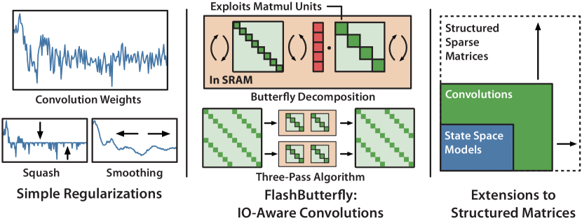
Figure 1: Left: Simple regularization techniques allow long convolutions to match state space models in sequence modeling. Middle: FlashButterfly is an IO-aware algorithm for long convolutions that improves runtime performance and scales to long sequences. Right: We show deep connections to advances in block-sparse matrix multiplication and structured matrices.

Closing the Quality Gap

First, to understand the quality gap, we study the performance of long convolutions compared to SSMs on Long Range Arena (LRA) [71], a key benchmark designed to test long sequence models. Long convolutions underperform SSMs by up to 16.6 points on average (Table 4). Visualizing the convolution kernels identifies a potential culprit: the long convolution kernels are non-smooth, whereas SSM kernels are smooth (Figure 2).

We explore two simple regularization techniques from the signal processing literature that alleviate this problem. The first technique uses a Squash operator to reduce the magnitude kernel weights in the time domain, enforcing sparsity that translates to smoothness in the frequency domain. The second technique applies a Smooth operator to the kernel weights in the time domain, which we find also promotes smoothness in the frequency domain. With regularization, long convolutions recover the performance of SSMs—and appear more robust to initialization than SSMs, matching S4 on LRA even with completely random initialization.

Motivated by the success of these simple regularizations on LRA, we further evaluate the performance of long convolutions on other complex sequence modeling tasks from diverse modalities. On image classification, we find that long convolutions can be an effective drop-in replacement for SSM layers. Replacing the SSM layer in S4 models with long convolutions yields a lift of 0.3 accuracy points on sequential CIFAR and comes within 0.8 points of S4ND-ISO on 2D CIFAR. On text modeling, long convolutions are competitive with the recent SSM-based H3 model [17]—coming within 0.3 PPL of H3 on OpenWebText [28] and matching H3 on the PILE [26]. Finally, long convolutions outperform both Transformers and SSMs in brain data modeling—by 0.14 and 0.16 MAE points, respectively—which suggests that the simpler architecture can even outperform SSMs for some applications.

Improving Runtime Performance

However, long convolutions are inefficient on modern hardware, since the FFT convolution incurs expensive GPU memory IO and cannot utilize matrix multiply units—even when using optimized implementations like cuFFT [56]. SSM convolution formulations rely on specialized GPU Cauchy kernels and Vandermonde kernels, as well as special recurrent message passing structure, to overcome these challenges.

In response, we develop FlashButterfly, a simple IO-aware algorithm for long convolutions, which does not require ad hoc hand engineering. FlashButterfly appeals to classic Butterfly decompositions of the FFT to rewrite the FFT convolution as a series of block-sparse Butterfly matrices. This decomposition reduces the number of passes over the input sequence—reducing the GPU memory requirements—and utilizes matrix multiply units on the GPU, which increases FLOP utilization.

FlashButterfly speeds up convolutions by 2.2$\times$ over cuFFT, and outperforms the fastest SSM implementations, since it does not incur the cost of generating the SSM convolution kernel. To demonstrate FlashButterfly’s scaling ability, we train a long convolution model on Path256, a task with sequence length 64K. We set state-of-the-art by 29.1 points and train 7.2$\times$ faster than the previous best model.

Deeper Connections and Learned Butterfly Extension

The Butterfly decomposition in FlashButterfly forms deep connections to recent work in block-sparse matrix multiplication [8]. Butterfly matrices are a special case of Monarch matrices, which capture a large class of structured matrices [15]. The block size $r$ interpolates between the fixed FFT for small block sizes to fully dense matrix multiplication for large matrices. This connection suggests a natural learned Butterfly extension that goes beyond convolutions in expressivity.

Our learned Butterfly extension simply learns the parameters in the Butterfly matrices from the data, instead of using the fixed matrices that corresopnd to the FFT and inverse FFT. Learning the Butterfly matrices while keeping the block size fixed yields additional parameters without additional FLOPS—yielding 0.8 additional points of lift on sequential CIFAR. Increasing the block size of the Butterfly matrices approaches the expressivity of fully dense matrices—including those used in linear layers and MLPs. As a proof of concept, we use this property to replace the MLPs in a Transformer language model—and outperform a GPT-2 model on WikiText103 by 0.2 PPL with 30% fewer parameters.

Summary

In summary, we show that long convolutions are an effective model for long sequence modeling. They match or exceed SSMs across an array of diverse sequence domains while requiring less hand-crafted initializations and showing improved stability. Additionally, by leveraging connections to Butterfly matrices, long convolutions can be trained up to 1.8$\times$ faster than SSMs.

2 Background

Deep State Space Models

A continuous-time state space model (SSM) maps an input signal $u(t)\in\mathbb{R}^{N}$, over time $t$, to an output signal $y(t)\in\mathbb{R}^{N}$ as

$$\dot{x}(t)= \mathbf{A}x(t)+\mathbf{B}u(t)$$

$$y(t)= \mathbf{C}x(t)+\mathbf{D}u(t),$$

by the use of hidden state $x(t)\in\mathbb{R}^{d}$ and some set of matrices $\mathbf{A}\in\mathbb{R}^{d\times d}$, $\mathbf{D}\in\mathbb{R}^{1\times 1}$, $\mathbf{B}\in\mathbb{R}^{d\times 1}$, $\mathbf{C}\in\mathbb{R}^{1\times d}$. Discretizing the SSM yields a recursion $x_{t}=\mathbf{A}x_{t-1}+\mathbf{B}u_{t}$, $y_{t}=\mathbf{C}x_{t}+\mathbf{D}u_{t}$. By unrolling the recursion, $y$ can be written as a convolution between $u$ and a kernel $\mathbf{K}$ that depends on $\mathbf{A}$, $\mathbf{B}$, $\mathbf{C}$:

$$y=\mathbf{K}\ast u+\mathbf{D}u.$$ (1)

A key ingredient to training deep SSM models is proper initialization of the learnable matrices $\mathbf{A}$, $\mathbf{B}$, $\mathbf{C}$, and $\mathbf{D}$. Initialization strategies often draw upon the HiPPO theory [29] on orthogonal polynomials, and involve the selection of measures and discretization strategies. The parameters may also be unstable to learn, which can require custom learning rate schedules [32].

FFT Convolution

Computing the convolution in Equation 1 can be costly for long sequences. A standard approach is to compute the convolution using the FFT convolution theorem. Then, the convolution can be computed as:

$$y=u\ast\mathbf{K}=\mathbf{F}_{N}^{-1}\mathbf{D}_{\mathbf{K}}\mathbf{F}_{N}u,$$ (2)

where $\mathbf{F}_{N}$ denotes the DFT matrix of size $N$, and $\mathbf{D}_{\mathbf{K}}=\text{diag}(\mathbf{F}_{N}\mathbf{K})$. This so-called FFT convolution scales in $O(N\log N)$ in sequence length $N$, but is often unoptimized on modern hardware (most optimized convolution operators focus on short convolutions, e.g., 3$\times$3).

Runtime Performance Characteristics

We provide a brief discussion of relevant factors affecting runtime performance. Depending on the balance of computation and memory accesses, operations can be classified as either compute-bound or memory-bound. In compute-bound operations, the time accessing GPU memory is relatively small compared to the time spent doing arithmetic operations. Typical examples are matrix multiply with large inner dimension, and short convolution kernels with a large number of channels. In memory-bound operations, the time taken by the operation is determined by the number of memory accesses, while time spent in computation is much smaller. Examples include most other operations: elementwise (e.g., activation, dropout) and reduction (e.g., sum, softmax, batch norm, layer norm).

Our Approach

Rather than parameterizing $\mathbf{K}$ with carefully initialized SSM matrices, we seek to directly parameterize the convolution $\mathbf{K}$ in Equation 1. Our goal is to replace the SSM layer with a learned convolution kernel as a drop-in replacement, while keeping the stacking and multi-head structure of SSM models (which can be thought of as multiple convolutional filters). We also aim to make the FFT convolution runtime-performant on modern hardware.

3 Method

Table 1: Accuracy on the ListOps task in LRA.

Model	Accuracy
S4-LegS	59.6
Long Convs	53.4
Long Convs, +Smooth	59.8
Long Convs, +Squash	60.3
Long Convs, +Squash, +Smooth	59.7

In Section 3.1, we conduct an initial investigation into long convolutions for sequence modeling, and develop two simple regularization strategies based on our findings. Then, in Section 3.2, we present FlashButterfly, an IO-aware algorithm for speeding up convolutions modeled after block-sparse matrix multiplication. Finally, we present an extension of FlashButterfly that leverages the block-sparse connection for additional expressivity.

3.1 Long Convolutions for Sequence Modeling

First, we conduct a brief investigation into the performance of vanilla long convolutions on sequence modeling, and we find a gap in quality. We then propose two simple regularization techniques for closing this gap.

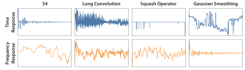
Figure 2: Visualizations of kernels trained on the ListOps task in LRA. Left to right, top to bottom: S4, long convolutions without regularization, long convolutions with the Squash operator, and long convolutions with the Smooth operator. Time response on top, frequency response on the bottom.

Motivation for Regularization: Non-Smooth Kernels

We begin by directly replacing the SSM layers in an S4 model with long convolutions, with random initialization. We train a model on the ListOps task from the long range arena (LRA) benchmark [71], with element-wise dropout on the convolution kernel weights. Table 1 shows that long convolutions underperform SSMs with 6.2 points on ListOps.

To understand the gap in performance, we visualize one head of the convolution kernel $\mathbf{K}$, compared to an SSM kernel in Figure 2. Compared to well-initialized SSM kernels, we find that directly learning convolution weights results in convolution kernels that are non-smooth and appear noisy. We hypothesize that these properties are responsible for the performance gap.

Table 2: Convolution- and SSM-specific hyperparameters.

Model	Hyperparameters	Initializations
SSM	$d$, $lr_{A}$, $lr_{B}$, $lr_{C}$	LegS, FouT, LegS/FouT
	dropout, discretization	Inv, Lin
Long Convs	$\lambda$, kernel LR,	Random, Geometric
	k, dropout

Regularizing the Kernel

We propose two simple techniques for regularizing the convolution kernel to alleviate these issues: Squash and Smooth. The Squash operator is applied element-wise to the convolution kernel, and reduces the magnitude of all weights: $\overline{\mathbf{K}}=\text{sign}(\mathbf{K})\odot\text{max}(|\mathbf{K}|-\lambda,0)$. As an aside, we note that Squash is equivalent to taking one step of an L1 proximal operator: $\overline{\mathbf{K}}=\operatorname{Prox}_{\lambda\|.\|}(\mathbf{K})=\operatorname{argmin}_{x}\{\lambda\lVert x\rVert_{1}+\lVert x-\mathbf{K}\rVert_{2}^{2}\}$ and thus may have principled connections to proximal gradient techniques. The Smooth operator applies simple average pooling, with width $p$, to the convolution kernel: $\overline{\mathbf{K}}_{k}=(2p+1)^{-1}\sum_{j=1}^{2p+1}\mathbf{K}_{k+j-p}.$

Training long convolutions with these regularizations matches SSMs in performance on the ListOps task (Table 1). Additionally, Figure 2 right shows that these regularizations improve smoothness in the frequency domain as well. In Appendix B, we evaluate directly smoothing in frequency domain.

Initialization

We seek to understand how sensitive long convolutions are to initialization. We note that since $\mathbf{K}$ directly parameterizes the convolution kernel, we can also leverage advances in initialization in SSMs such as HiPPO [29] and S4-LegS [32]—simply by converting the initialized SSM model to a convolution kernel, and initializing $\mathbf{K}$ to the convolution weights.

While complex initialization strategies can be powerful, they require careful tuning to configure. To understand the impact of initialization on long convolutions, we evaluate two simple intialization techniques: random initialization, and a geometric decay initialization. The random initialization initializes the weights to be randomly distributed from a Normal distribution: $\mathbf{K}_{i}\sim\mathcal{N}$. The geometric decay initialization additionally scales kernel weights to decay across the sequence, as well as across the heads. For the kernel $\mathbf{K}^{(h)}$, $1\leq h\leq H$, we initialize the weights as: $\mathbf{K}^{(h)}_{k}=x\exp{(-kN^{-1}\left(H/2\right)^{hH^{-1}})},$ for $1\leq k\leq N$, where $x\sim\mathcal{N}$ is drawn from a Normal distribution.

Summary

The full method is written in Algorithm 1, with a forward reference to our fast convolution solution FlashButterfly. In Algorithm 1, all operators ($\operatorname{max}$, $\operatorname{sign}$, and absolute value) are applied entry-wise, FlashButterfly is taken over the sequence dimension and the skip connection is taken over the head dimension.

Algorithm 1 Regularized Long Convolution

0:  Input $u\in\mathbb{R}^{B\times H\times N}$, $\mathbf{K}\in\mathbb{R}^{H\times N}$, $\mathbf{D}\in\mathbb{R}^{H}$, where $N$ is the sequence length, $H$ is the head dimension, and $B$ is the batch size.

1:  $\mathbf{K}\leftarrow\operatorname{dropout}(\mathbf{K})$.

2:  $\mathbf{K}_{k}\leftarrow(2p+1)^{-1}\sum_{j=1}^{2p+1}\mathbf{K}_{k+j-p}$.

3:  ${\mathbf{K}}\leftarrow\text{sign}(\mathbf{K})\odot\text{max}(|\mathbf{K}|-\lambda,0)$.

4:  $y\leftarrow\textsc{FlashButterfly}(\mathbf{K},u)+\mathbf{D}\odot u.$

5:  Return $y\in\mathbb{R}^{B\times H\times N}$

Convolution-specific hyperparameters are shown in Table 2. Compared to the hyperparameters necessary to train S4, our regularization approaches have fewer hyperparameters and choices than S4.

3.2 FlashButterfly

In addition to improving the quality of long convolutions, it is also critical to improve runtime performance. We present FlashButterfly, an IO-aware algorithm for speeding up general convolutions on modern hardware. We use kernel fusion to reduce GPU memory IO requirements, and use a Butterfly decomposition to rewrite the FFT as a series of block-sparse matrix multiplications. To scale to long sequences, we use an alternate Butterfly decomposition to construct a three-pass FFT convolution algorithm to further reduce IO requirements.

Kernel Fusion

Naive implementations of the FFT convolution incur expensive GPU memory IO. The FFT, inverse FFT, and pointwise multiplication in Equation 2 each require at least one read and write of the input sequence from GPU memory. For long sequences, the IO costs may be even worse: the entire input sequence cannot fit into SRAM, so optimized implementations such as cuFFT [56] must take multiple passes over the input sequence using the Cooley-Tukey decomposition of the FFT [11]. Following FlashAttention [16], FlashButterfly’s first fuses the entire FFT convolution into a single kernel to compute the entire convolution in GPU SRAM and avoid this overhead.

Butterfly Decomposition

Kernel fusion reduces the IO requirements, but the fused FFT operations still cannot take full advantage of specialized matrix multiply units on modern GPUs, such as Tensor Cores on Nvidia GPUs, which perform fast 16 $\times$ 16 matrix multiplication. We appeal to a classical result, known as the four-step or six-step FFT algorithm [4], that rewrites the FFT as a series of block-diagonal Butterfly matrices [61] interleaved with permutation.

The Butterfly decomposition states that we can decompose an $N$-point FFT into a series of FFTs of sizes $N_{1}$ and $N_{2}$, where $N=N_{1}N_{2}$. Conceptually, the algorithm reshapes the input as an $N_{1}\times N_{2}$ matrix, applies $N_{1}$ FFTs of size $N_{2}$ to the columns, multiplies each element by a twiddle factor, and then applies $N_{2}$ FFTs of size $N_{1}$ to the rows.

More precisely, let $\mathbf{F}_{N}$ denote the DFT matrix corresponding to taking the $N$-point FFT. Then, there exist permutation matrices $\mathbf{P}$, and a diagonal matrix $\mathbf{D}$, such that $\mathbf{F}_{N}=\mathbf{P}(\mathbf{I}_{N_{2}}\otimes\mathbf{F}_{N_{1}})\mathbf{P}^{T}\mathbf{D}(\mathbf{I}_{N_{1}}\otimes\mathbf{F}_{N_{2}})\mathbf{P}$. $\mathbf{P}$ denotes a permutation matrix that reshapes the input to $N_{1}\times N_{2}$ and takes the transpose, $\mathbf{D}$ denotes a diagonal matrix with the twiddle factors along the diagonal, $\otimes$ denotes the Kronecker product, and $vI_{N_{i}}$ and $\mathbf{F}_{N_{i}}$ are the identity and DFT matrices of size $N_{i}\times N_{i}$. Precise values for $\mathbf{F}_{N_{i}}$, $\mathbf{D}$, and $\mathbf{P}$ are given in Appendix C.

The Butterfly decomposition incurs $O(Nr\log N/\log r)$ FLOPS for a sequence length $N=r^{p}$, with block size $r$. In general FFT implementations, $N$ is typically padded to a power of two, so that the block size can be set to $2$ to minimize the total number of FLOPS. However, on GPUs with a specialized $b\times b$ matrix multiply unit, the FLOP cost of computing an $r\times r$ matrix multiply with $r<b$ is equivalent to performing a single $b\times b$ matrix multiply. Thus, the actual FLOP count scales as $O(Nb\log N/\log r)$ for $r<b$. Increasing the block size up to $b$ actually reduces the FLOP cost.

Table 3 demonstrates this tradeoff on an A100 GPU, which has specialized matrix multiply units up to 16 $\times$ 32. Runtime decreases as $r$ increases from 2, even though theoretical FLOPS increase. Once $r>b$, runtime begins increasing as actual FLOPS increase as well.

Table 3: Runtime, GLOPs, and FLOP util for the Butterfly decomposition with different block sizes $r$ for sequence length 4096, on A100 with batch size $128$, head dimension $32$.

Block Size	Runtime (ms)	GLOPs	FLOP Util
2	0.52	2.0	1.3%
16	0.43	8.1	6.0%
64	0.53	21.5	13.0%
256	0.68	64.5	30.4%

Three-Pass Algorithm

Kernel fusion and the Butterfly decomposition improve runtime performance, but only for convolutions short enough to fit into SRAM (length 8K or shorter on A100). For longer sequences, we again appeal to the Butterfly decomposition, but using an alternate formulation that eliminates permutations over the input sequence. This formulation allows us to decompose the convolution into three passes over the data: a Butterfly matrix multiplication that can be computed with a single IO, FFT convolutions that we can compute in parallel, and a final Butterfly matrix multiplication that can also be computed with a single IO.

In particular, we rewrite the DFT matrix $\mathbf{F}_{N}$ of size $N$ as $N\mathbf{P}^{-1}(\mathbf{I}_{m}\otimes(l\mathbf{F}_{l}))\overline{\mathbf{B}}^{-1},$ and its inverse matrix $\mathbf{F}_{N}^{-1}$ as $N^{-1}\overline{\mathbf{B}}(\mathbf{I}_{m}\otimes\overline{\mathbf{F}}_{l})\mathbf{P}$, where $\mathbf{B}$ is an $N\times N$ block matrix with $m^{2}$ blocks of size $l\times l$, each of which is diagonal (see Appendix C for the exact derivation). Critically, matrix-vector multiply $\mathbf{B}u$ can be computed in a single pass over the input vector $u$. Substituting these into Equation 2 and simplifying yields the following:

$$y=u\ast\mathbf{K}=\overline{\mathbf{B}}(\mathbf{I}_{m}\otimes\overline{\mathbf{F}}_{l})\mathbf{D}^{\prime}_{\mathbf{K}}(\mathbf{I}_{m}\otimes\mathbf{F}_{l})\overline{\mathbf{B}}^{-1},$$ (3)

where $\mathbf{D}^{\prime}_{\mathbf{K}}=l\mathbf{P}\mathbf{D}_{\mathbf{K}}\mathbf{P}^{-1}$ is another diagonal matrix. The middle terms can now be computed as $m$ independent FFT convolutions of size $l$, with a different convolution kernel. These parallel convolutions collectively require one pass over $N$ input elements, so the entire convolution can be computed with three passes over the input.

The full algorithm for FlashButterfly for $N>l$ is shown in Algorithm 2.

Algorithm 2 FlashButterfly

0:  Input $u\in\mathbb{R}^{B\times H\times N}$, $\mathbf{K}\in\mathbb{R}^{H\times N}$, $\mathbf{D}\in\mathbb{R}^{H}$, where $N=lm$ is the sequence length, $H$ is the head dimension, and $B$ is the batch size.

1:  $\hat{\mathbf{K}}\leftarrow FFT(\mathbf{K})$

2:  $\mathbf{D}^{\prime}_{\mathbf{K}}\leftarrow\mathbf{P}(\hat{\mathbf{K}})\mathbf{P}^{-1}$

3:  $u\leftarrow\overline{\mathbf{B}}^{-1}u$

4:  Compute $u\leftarrow(\mathbf{I}_{m}\otimes\overline{\mathbf{F}}_{l})\mathbf{D}^{\prime}_{\mathbf{K}}(\mathbf{I}_{m}\otimes\mathbf{F}_{l})u$ in parallel across $m$ streaming multiprocessors

5:  Return $\overline{\mathbf{B}}u\in\mathbb{R}^{B\times H\times N}$

We show that Algorithm 2 is correct, and that it can be computed in three passes over the input sequence. The proof is given in Appendix D.

Proposition 1.

Algorithm 2 computes the convolution $u\ast\mathbf{K}$ with at most three passes over the input sequence $u$.

3.2.1 Learned Butterfly Extension

The Butterfly decomposition in FlashButterfly suggests a natural extension: learning the values of the Butterfly matrices $\mathbf{F}_{r}$ in the Butterfly decomposition, instead of using the fixed matrices corresponding to the FFT. If we keep the block size $r$ fixed, then the number of parameters in the Butterfly matrices increases by $O(Hr^{2})$, but the total FLOPS in the model stay the same. Increasing the block size allows us to further increase expressivity, but at additional compute cost. As $r$ approaches $N$, the Butterfly decomposition approaches the compute cost and expressivity of a full dense matrix multiply: $O(N^{2})$.

4 Evaluation

We evaluate how well long convolutions perform in a variety of challenging sequence modeling tasks from diverse modalities and benchmarks, including the long range arena benchmark, image classification, text modeling, and brain data modeling (Section 4.1). We find that long convolutions are strong sequence modelers across these tasks. Next, we evaluate the runtime performance of long convolutions under FlashButterfly and evaluate how well it scales to very long sequences (Section 4.2). Finally, we evaluate the quality improvements from learned Butterfly extension (Section 4.3).

Table 4: Validation accuracy of different models on the LRA benchmark. Best in bold, second best underlined.

Model	ListOps	Text	Retrieval	Image	Pathfinder	Path-X	Avg
Transformer	36.4	64.3	57.5	42.4	71.4	✗	53.7
Nyströmformer	37.2	65.5	79.6	41.6	70.9	✗	57.5
Reformer	37.3	56.1	53.4	38.1	68.5	✗	50.6
BigBird	36.1	64.0	59.3	40.8	74.9	✗	54.2
Linear Trans.	16.1	65.9	53.1	42.3	75.3	✗	50.5
Performer	18.0	65.4	53.8	42.8	77.1	✗	51.2
S4-LegS	59.6	86.8	90.9	88.7	94.2	96.4	86.1
S4-FouT	57.9	86.2	89.7	89.1	94.5	✗	77.9
S4-LegS/FouT	60.5	86.8	90.3	89.0	94.4	✗	78.5
S4D-LegS	60.5	86.2	89.5	88.2	93.1	92.0	84.9
S4D-Inv	60.2	87.3	91.1	87.8	93.8	92.8	85.5
S4D-Lin	60.5	87.0	91.0	87.9	94.0	✗	78.4
S4 (Original)	58.4	76.0	87.1	87.3	86.1	88.1	80.5
Long Conv, Rand	53.4	64.4	83.0	81.4	85.0	✗	69.5
Long Conv, Rand + Smooth	59.8	68.7	86.6	79.3	86.1	✗	71.8
Long Conv, Rand + Squash	60.3	87.1	90.0	88.3	94.0	96.9	86.1
Long Conv, Rand + Squash + Smooth	59.7	72.8	88.6	80.8	90.1	✗	73.7
Long Conv, Exp + Squash	62.2	89.6	91.3	87.0	93.2	96.0	86.6

Table 5: Image classification on flattened images.

Model	sCIFAR
Transformer	62.2
LSTM	63.0
r-LSTM	72.2
UR-LSTM	71.0
UR-GRU	74.4
HIPPO-RNN	61.1
LipschitzRNN	64.2
CKConv	64.2
S4-LegS	91.8
S4-FouT	91.2
S4D-LegS	89.9
S4D-Inv	90.7
S4D-Lin	90.4
Long Conv, Random	91.0
Long Conv, Geom Init	92.1

Table 6: Image classification on 2D images.

Model	CIFAR
S4ND-ISO	89.9
Long Conv 2D-ISO, Rand init	88.1
Long Conv 2D-ISO, Geom init	89.1

Table 7: Test PPL of models trained on OpenWebText.

Model	Test PPL
Transformer	20.6
S4D	24.9
GSS	24.0
H3	19.6
H3 + Long-Conv, Rand Init	20.1
H3 + Long-Conv, Geom Init	19.9

Table 8: Test PPL on the Pile for models trained with various tokens.

Train Tokens	5B	10B	15B
Transformer	12.7	11.3	10.7
H3	11.8	10.7	10.2
H3 + Long Convs, Geom Init	11.9	10.7	10.3

Table 9: Evaluation on brain fMRI data.

Model	MAE
Transformer	0.68
H3	0.70
H3 + Long Convs, Rand Init	0.58
H3 + Long Convs, Geom Init	0.54

4.1 Quality on Sequence Modeling

In this section, we evaluate the performance of long convolutions in sequence modeling in terms of quality. We begin by evaluating various regularization and initialization techniques on the long range arena benchmark, a suite of general-purpose sequence modeling tasks designed to stress test long sequences [71]. We take the best-performing variants and move on to two challenging and diverse modalities that have been used to evaluate sequence models, including SSMs: image classification (both one-dimensional and two-dimensional) and text modeling. We conclude the section with a real-world application of long convolutions to brain data modeling.

We find that long convolutions perform well across all of these diverse tasks and modalities—and are generally more robust to choice of initialization than SSMs. Our results suggest that long convolutions may be a compelling simpler alternative to SSMs for sequence modeling. Experimental details for the tasks are given in Appendix F, and additional experiments are provided in Appendix B.

4.1.1 Long Sequence Modeling: Long Range Arena

We first evaluate long convolutions on Long Range Arena (LRA), a benchmark suite used to test general-purpose sequence modeling over long contexts. LRA consists of six long-range sequence modeling tasks, with sequence lengths between 1K and 16K tokens. The tasks have modalities including text, natural and synthetic images, and mathematical expressions. We take the state-of-the-art S4 architecture [32], and replace the SSM layers with long convolutions.

We present five variants of long convolutions: random intialization and no regularization, random initialization with the Smooth operator, random initialization with the Squash operator, random initialization with both operators, and the geometric initialization with the Squash operator. We compare the long convolution methods against variants of Transformers presented in the original Long Range Arena paper [71], as well as variants of S4 with different parameterizations and initializations [32]. These initializations are important for S4 to achieve high quality.

Table 4 shows the results for long convolutions on the LRA benchmark. An ✗ in the Path-X column indicates that the model never achieved better classification accuracy than random guessing. Long convolutions appear to be robust to initialization: there is only a 0.5 point spread in the average score between long convolutions with a geometric initialization and long convolutions with a random initialization—though individual tasks may have more spread. This stands in contrast to the S4 methods, which are sensitive to initialization choices and the parameterization—with a spread of 7.6 points between S4-LegS and S4-LegS/FouT.

Regularization is critical for achieving strong performance; without it, long convolutions lose 17.1 points on average across the six LRA tasks. Using the Squash operator on its own appears to perform better than using the Smooth operator, or using both together. For the rest of the experiments, we focus on the two best-performing variants of long convolutions: random initialization with the Squash operator, and geometric initialization with the Squash operator.

4.1.2 Image Classification

Next, we evaluate long convolutions on image classification. We evaluate two settings which have been used to evaluate SSMs and sequence models: 1D pixel-by-pixel image classification, and 2D image classification. These settings are challenging for sequence modeling, as they require modeling complex spatial relationships between image pixels in a continuous space. For the 1D case, we again use long convolutions as a drop-in replacement for the SSM layer in the state-of-the-art S4 architecture. For the 2D case, we replace the S4 layers in S4ND [53] with 2D long convolution filters.

Tables 6 and 6 show the results. On 1D image classification, long convolutions again match the performance of S4, even with random initializations, while their performance improves further by 1.1 points when using the geometric initialization. On 2D image classification, long convolutions come within 0.8 points of the state-of-the-art S4ND model. Further regularization or inductive bias may be helpful for long convolutions to recover the performance of SSMs in higher dimensions.

4.1.3 Text Modeling: OpenWebText and the PILE

We evaluate long convolutions on text modeling. Text has been a challenging modality for state space models and non-attention sequence models, since it requires comparing and copying elements across the input sequence [17, 58]. We build off of the H3 model [17]—the state-of-the-art SSM model for text modeling—which stacks two SSMs and multiplies their outputs together as a gating mechanism. We use long convolutions as a drop-in replacement for the SSMs in the H3 layer.

Following the H3 paper, we keep two attention layers in the overall language model and evaluate on two datasets: OpenWebText [28] and the Pile [26]. We use OpenWebText to evaluate the role of initialization: we train models to completion at 100B tokens, and evaluate both random and geometric initializations. For the Pile, we evaluate how well long convolutions scale with data: we use the geometric initialization, and evaluate the performance of models trained with 5B, 10B, and 15B tokens.

Tables 8 and 8 show the results. On OpenWebText, long convolutions with random initialization come within 0.5 PPL points of H3, and the geometric decay initialization comes within 0.3 PPL. Both models outperform the Transformer. On the Pile, long convolutions with geometric decay initialization nearly match H3 everywhere along the data scaling curve, and outperform Transformers. These initial results suggests that convolutions—with some multiplicative gating mechanism—may be a promising candidate for language modeling.

4.1.4 Brain fMRI Analysis

Finally, we evaluate long convolutions on a real-world sequence modeling modality: analysis of brain functional Magnetic Resonance Imaging (fMRI) sequence data. To this end, we replicate the self-supervised pre-training task proposed by Thomas et al. [72]: training models to predict whole-brain activity for the next time step of an fMRI sequence (using a large-scale upstream dataset, spanning fMRI data from $11,980$ experimental runs of $1,726$ individuals). We compare long convolutions against Transformers and H3, architectures that achieve state-of-the-art performance in this task [72, 17], by adapting the H3 model and replacing the SSM kernel with long convolutions. Long convolutions outperform the other models in accurately predicting brain activity in this task (see Table 9). Full details of this analysis are provided in Appendix F.1, where we also show that long convolutions perform on par with the other models in accurately classifying new fMRI sequences in a downstream adaptation.

4.2 Efficiency: FlashButterfly

Table 10: LRA Speed Benchmark.

Model	Speedup
Transformer	1$\times$
FlashAttention	2.4$\times$
SSM + FlashConv	5.8$\times$
FlashButterfly	7.0$\times$

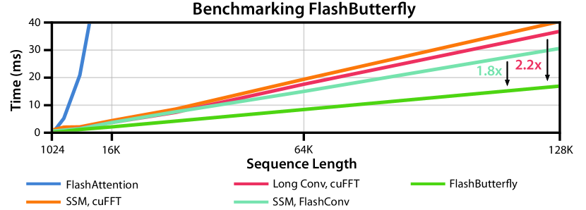
Figure 3: We compare the performance of FlashButterfly to attention, SSMs with cuFFT, long convolutions with cuFFT, and SSMs with FlashConv, the most optimized SSM algorithm [17]. Speedups shown for sequence length 128K.

Table 11: Runtime and accuracy on Path256 (sequence length 64K).

Model	Accuracy	Training Time
Transformer	✗	✗
FlashAttention	✗	✗
Block-Sparse FlashAttention	63.1	3 days
FlashButterfly	92.2	10 hours

We now turn towards evaluating the runtime performance of FlashButterfly. We focus on two questions: whether FlashButterfly can outperform SSMs in terms of runtime performance, and how well FlashButterfly can scale to long sequences. First, we evaluate FlashButterfly’s runtime on the Long Range Arena speed benchmark [71], which measures runtime on a byte-level text classification benchmark that is representative of standard sequence modeling loads. FlashButterfly outperforms SSMs and baselines from the original LRA speed benchmark. Next, we evaluate how well FlashButterfly scales to longer sequences. Across many sequence lengths, FlashButterfly outperforms the fastest SSM implementation. Finally, we demonstrate FlashButterfly’s sequence scaling capabilities on an extremely long sequence task: Path256, which has sequence length 64K.

4.2.1 Runtime on Long Range Arena

We begin by evaluating runtime on the Long Range Arena speed benchmark [71]. The benchmark measures runtime on a byte-level text classification task. This task, which has sequence length 4K, is representative of typical sequence modeling training workloads, and is a standard evaluation benchmark for Transformers and SSMs [71]. The benchmark is measured in terms of speedup against vanilla Transformers using a HuggingFace implementation. We additionally compare against two more baselines: a) Transformers using FlashAttention [16], the fastest attention algorithm, and b) SSMs using FlashConv [17], the fastest SSM implementation.

Table 10 shows the results. FlashButterfly achieves 7.0$\times$ speedup over the Transformer baseline. It outperforms FlashAttention, since its compute scales nearly linearly with sequence length instead of quadratically. It also outperforms FlashConv, the fastest SSM implementation, since it does not require kernel generation. These results show that FlashButterfly outperforms SSMs and Transformers in terms of runtime efficiency in standard sequence modeling workloads.

4.2.2 Scaling to Longer Sequences

Next, we evaluate how well FlashButterfly scales to longer sequence lengths. We compare FlashButterfly against a) convolutions using cuFFT, the standard implementation in PyTorch, and b) SSMs using FlashConv. We measure the runtime for sequence lengths ranging from 1K to 128K. Following [17], we measure the runtime of a single layer using batch size 32 and 128 model dimension. We also provide attention runtime, as well as SSMs using a standard PyTorch implementation, for context.

Figure 3 shows the results. FlashButterfly yields up to 2.2$\times$ speedup against baseline cuFFT-based convolutions. FlashButterfly outperforms FlashConv for all sequence lengths, since it does not require the kernel generation step of SSMs. These results show that FlashButterfly outperforms SSMs and Transformers across all sequence lengths—even very long sequences.

We demonstrate the utility of FlashButterfly by training models on a task with extremely long sequences: Path256, which has sequence length 64K. Table 11 shows that long convolutions achieve state-of-the-art performance on Path256, outperforming block-sparse FlashAttention from [16], the only prior work to report non-trivial performance ($>$50% accuracy) on Path256. Long convolutions with FlashButterfly exceed state-of-the-art performance by 29.1 points, and train 7.2$\times$ faster.

4.3 Learned Butterfly Extension

Table 12: Performance with learnable Butterfly of different sizes

Block Size	sCIFAR	Speedup
Fixed Butterfly	91.0	1$\times$
16	91.8	1$\times$
32	92.4	0.9$\times$
256	92.5	0.6$\times$

Table 13: Performance of replacing MLPs with the long conv extension in a Transformer on WikiText103.

Model	PPL	Params
GPT-2-Small	20.6	124M
Monarch-GPT-2-Small	20.7	72M
FlashButterfly-GPT-2-Small	20.4	86M

Finally, we experimentally evaluate how well the learned Butterfly extension can improve quality on two tasks: sequential CIFAR and WikiText103.

First, on sequential CIFAR, we use the same architecture as in Section 4.1, except with learned Butterfly matrices. Table 13 shows the results for sequential CIFAR, with varying block sizes. Block size 16 yields lift over the baseline with fixed Butterfly matrices, without sacrificing runtime. Larger block sizes yield further lift, but at the cost of additional runtime.

Next, on WikiText103, we evaluate the learned Butterfly extension in an alternate setting: replacing MLPs in a Transformer, following [15]. In this setting, we leverage the fact that a Butterfly matrix with large block size (256) approximates a dense matrix multiplication, but has fewer parameters. We compare our learned Butterfly extension against a Transformer with dense MLPs, and against Transformers where the MLPs have been replaced with Monarch matrices [15]. The metric is whether we can achieve the same performance as a Transformer with dense MLPs, but with fewer parameters.

Table 13 shows the results. Our extension outperforms both the baseline Transformer and Monarch, outperforming the Transformer with a 30% reduction in parameters. This result validates the connection between our learned Butterfly extension and structured sparse matrices.

5 Conclusion

We find that regularizing the kernel weights with a squash operator allows long convolutions to achieve strong performance on a variety of long sequence modeling tasks. We develop FlashButterfly to improve the runtime efficiency of long convolutions, using Butterfly decompositions, and we connect convolutions to recent advances in block-sparse matrix multiplication.

Appendix A Related Work

State space models

Following S4 [30], deep state space models have been demonstrating promise in sequence modeling. These models have been especially promising for long sequences, which are challenging for architectures such as Transformers [75], and has required custom approaches to adapt to higher-dimensional data [20, 47] or long sequences [13, 76]. Deep SSMs have shown state-of-the-art performance on a number of domains, including time series data [77, 30, 79], audio [27], visual data [53], text [50, 51, 17], and medical data [70]. A number of methods have also been proposed to simplify the S4 architecture in parameterization [34, 31, 68], make the parameterization more numerically stable [27], or improve the initialization [32]. Some of these approaches have also combined SSMs with other sequence modeling primitives [37], including attention [50, 51, 17], and Goel et al. [27] have used SSMs as a drop-in replacement in audio generation models. Our work is complementary to these approaches. For example, one way to leverage principled initialization techniques is to apply them directly to the long convolutions. Our work also suggests that long convolutions may be promising architectures for the downstream applications where SSMs have shown strong performance.

Convolutions

Convolutions have a long history in signal processing [69] and machine learning, especially in computer vision [38, 42, 43]. Most models are based on short, localized convolutions [73], and most libraries are optimized for short convolutions [62]. Recently, in conjunction with the development of state space models, there has been growing interesting in models that use long convolutions [64, 65, 74], often with implicit representations [46, 33, 44]. Approaches such as CKConv [65] and SGConv [46] have shown that convolutions can be effective for sequence modeling, but require parameter counts that grow sub-linearly in sequence length and build in explicit biases into the parameterization [46]. Our work provides additional support for the use of long convolutions for sequence modeling, and suggest that—with the right regularization—long convolutions can be used successfully for sequence modeling without controlling for parameter counts.

FFT Algorithms

The computational feasibility of long convolution models depends on the Fast Fourier Transform (FFT). The Cooley-Tukey FFT algorithm, published in 1965 [11], enabled convolution and Fourier transforms to scale in the length dimension from $O(N\log N)$ instead of $O(N^{2})$. Subsequently, many alternative algorithms for efficiently computing the Fourier transform have emerged, including algorithms for computing the FFT in parallel [2]. These algorithms have enabled fundamental progress in a range of disciplines, including control theory [7, 6] and signal processing [59, 60]. A survey of methods is included in Chu & George, Bahn et al..

As FFTs prove more useful for modern deep learning workloads—e.g., through long convolutions—new techniques are required to run them efficiently. Of particular interest to our work is making FFTs run efficiently on GPUs with specialized matrix multiplication units, such as tensor cores. For example, an A100 GPU has a maximum of 312 TFLOPs/s of FP16 with tensor cores, but only 20 TFLOPs/s of FP32 (and 40 TFLOPs/s of FP16) without tensor cores [55]. This trend started with the V100 GPUs [54] and has continued with the H100 GPUs [57]. Our work is related to and draws from efforts in the high-performance computing community to accelerate FFTs given these new hardware primitives [45], but focuses specifically on using them in convolutions. In the convolution workload, it is important to mitigate IO costs and increase FLOP utilization in concert.

Sparse Structured Matrices

Sparse structured matrices have recently received a great deal of attention as a promising research topic in making machine learning models more runtime- and parameter-efficient. Sparse training has a long history in machine learning, including work in pruning neural networks [35, 36, 66, 48, 19] and finding lottery tickets [23, 24, 25]. Structured matrices are another approach to making models more efficient. Structured matrices have subquadratic ($o(n^{2})$ for dimension $n\times n$) parameters and runtime, such as sparse and low-rank matrices, and fast transforms (Fourier, Chebyshev, sine/cosine, orthogonal polynomials) [15]. Critically, simple divide-and-conquer schemes can lead to fast algorithms for many structured matrices [18], and structured matrices can be used to represent many commonly used fast transforms [67, 40, 21]. Our connection to these matrices comes through butterfly matrices [14, 8, 61], which have been shown to be expressive and hardware-efficient [15]. Butterfly matrices have also been used in kernel methods [9, 52] and deep learning methods [63, 49, 1], which may suggest other fruitful avenues of future work for long convolutions with a learned Butterfly formulation. Our work suggests that using long convolution models may offer an inroads to utilizing structured matrices in deep learning.

Appendix B Additional Experiments

B.1 Regularization in Frequency Domain

Table 14: Validation accuracy of different models on the LRA benchmark. This table includes extra experiments where we run the Smooth operator over the frequency domain. Best in bold, second best underlined.

Model	ListOps	Text	Retrieval	Image	Pathfinder	Path-X	Avg
Transformer	36.4	64.3	57.5	42.4	71.4	✗	53.7
Nyströmformer	37.2	65.5	79.6	41.6	70.9	✗	57.5
Reformer	37.3	56.1	53.4	38.1	68.5	✗	50.6
BigBird	36.1	64.0	59.3	40.8	74.9	✗	54.2
Linear Trans.	16.1	65.9	53.1	42.3	75.3	✗	50.5
Performer	18.0	65.4	53.8	42.8	77.1	✗	51.2
S4-LegS	59.6	86.8	90.9	88.7	94.2	96.4	86.1
S4-FouT	57.9	86.2	89.7	89.1	94.5	✗	77.9
S4-LegS/FouT	60.5	86.8	90.3	89.0	94.4	✗	78.5
S4D-LegS	60.5	86.2	89.5	88.2	93.1	92.0	84.9
S4D-Inv	60.2	87.3	91.1	87.8	93.8	92.8	85.5
S4D-Lin	60.5	87.0	91.0	87.9	94.0	✗	78.4
S4 (Original)	58.4	76.0	87.1	87.3	86.1	88.1	80.5
Long Conv, Rand	53.4	64.4	83.0	81.4	85.0	✗	69.5
Long Conv, Rand + Smooth	59.8	68.7	86.6	79.3	86.1	✗	71.8
Long Conv, Rand + Smooth, Freq	56.1	67.9	86.8	85.2	88.3	✗	72.4
Long Conv, Rand + Squash	60.3	87.1	90.0	88.3	94.0	96.9	86.1
Long Conv, Rand + Squash + Smooth	59.7	72.8	88.6	80.8	90.1	✗	73.7
Long Conv, Rand + Squash + Smooth, Freq	59.7	72.8	88.6	85.7	88.3	84.9	78.8
Long Conv, Exp + Squash	62.2	89.6	91.3	87.0	93.2	96.0	86.6

In earlier experiments, we also experimented with smoothing convolutions directly in the frequency domain. We convert the convolution kernel $\mathbf{K}$ to frequency domain with an FFT, apply the smoothing operator Smooth, and then convert it back to the time domain with an inverse FFT. Table 14 shows the results on LRA, with the convolutions smoothed in frequency domain denoted by “Smooth, Freq.” The performance is similar to smoothing in time domain, but underperforms using the Squash operator on its own, so we elected to just use the Squash operator in the remaining experiments.

B.2 Time Series Forecasting

Table 15: Univariate long sequence time-series forecasting results on ETTh1 Informer benchmark. Comparisons across five horizon prediction settings. Best mean squared error (MSE) and mean absolute error (MAE) in bold. Numbers reported from [30]. Long Convs outperforms S4 and obtains best MSE and MAE in four out of five evaluation settings.

Methods	Long Convs	S4	Informer	LogTrans	Reformer	LSTMa	DeepAR	ARIMA	Prophet
Metric	MSE MAE	MSE MAE	MSE MAE	MSE MAE	MSE MAE	MSE MAE	MSE MAE	MSE MAE	MSE MAE
24	0.06 0.20	0.06 0.19	0.10 0.25	0.10 0.26	0.22 0.39	0.11 0.27	0.11 0.28	0.11 0.28	0.12 0.28
48	0.07 0.21	0.08 0.22	0.16 0.32	0.17 0.33	0.28 0.45	0.19 0.36	0.16 0.33	0.18 0.42	0.17 0.33
168	0.07 0.21	0.10 0.26	0.18 0.35	0.21 0.38	1.52 1.19	0.24 0.39	0.24 0.42	0.40 0.50	1.22 0.76
336	0.08 0.23	0.08 0.23	0.22 0.39	0.23 0.40	1.86 1.12	0.59 0.70	0.45 0.55	0.47 0.59	1.55 1.82
720	0.09 0.24	0.12 0.27	0.27 0.44	0.27 0.46	2.11 1.44	0.68 0.77	0.66 0.71	0.66 0.77	2.74 3.25

Time series forecasting is another challenging modality for sequence modeling, which requires reasoning over multiple time contexts. We evaluate the performance of long convolutions on different future horizon prediction windows in ETTh₁, a real-world long sequence time series forecasting task from the Informer benchmark [78]. Following the original S4 paper, we evaluate on the univariate ETTh₁ task, which involves predicting electricity transformer temperature at hour-long granularities (i.e., 24, 48, 168, 336, and 720 hours in the future). For each prediction task, we use the same number of hours before as a look-back window to input to the model. As LongConvs can be a drop-in replacement for the S4 kernel, we also follow the approach taken in S4 that simply masks out the future time steps in the input sequence and treat the task as a masked sequence-to-sequence transformation. Table 15 shows the results. Long convolutions match or outperform S4 on all context windows, and outperforms custom hand-crafted architectures designed specifically for time series forecasting.

B.3 Brain fMRI Downstream Adaptation

Table 16: Downstream performance on brain fMRI data.

Dataset	Model	F1
MDTB	Transformer	91.8
	H3	92.0
	H3 + Long Convs, Rand Init	92.1
	H3 + Long Convs, Exp Init	91.6
HCP	Transformer	83.4
	H3	82.6
	H3 + Long Convs, Rand Init	82.3
	H3 + Long Convs, Exp Init	83.6

We further evaluate the performance of the pre-trained models in two benchmark mental state decoding datasets from the Human Connectome Project [HCP; 5] and multi-domain task battery [MDTB; 41], spanning $20$ and $26$ distinct mental states respectively. To adapt the pre-trained models to the mental state decoding (i.e., classification) task, we add a learnable classification embedding $E^{cls}\in\mathbb{R}^{n}$ to the end of input sequences $X$ and forward the model’s corresponding prediction to a decoding head $p(\cdot)$, composed of a dense hidden layer with $e$ model units (one for each embedding dimension, with $tanh$ activation) as well as a $softmax$ output layer (with one model unit $i$ for each considered mental state in the data). Accordingly, we adapt models by optimizing a standard cross entropy loss objective: $-\sum_{i}y_{i}\log\ {p(f(E^{X}))_{i}}$, where $y_{i}$ indicates a binary variable that is $1$ if $i$ is the correct mental state and $0$ otherwise. We always begin downstream adaptation with the pre-trained model parameters and allow all parameters to change freely during training. We randomly split each of the two downstream datasets into distinct training ($90\%$ of fMRI runs) and test ($10\%$ of fMRI runs) datasets and adapt models for $1,000$ training steps at a mini-batch size of $256$ and a learning rate of $5e^{-5}$ (otherwise using the same learning parameters as for upstream training). During training, we sample sequences from the fMRI datasets according to the accompanying event files, which specify the beginning and end of each experimental trial underlying a mental state [when accounting for the temporal delay of the haemodynamic response function; for details, see 72].

The adapted H3 variants with long convolutions perform on par with the other models in accurately identifying the mental states of the downstream evaluation datasets (see Table 16: F1-scores are macro-averaged).

Appendix C Methods Details

We discuss details of our methods.

C.1 Butterfly Decompositions

We describe how to construct $\mathbf{D}$ in the Butterfly decomposition, and $\mathbf{B}$ in the three pass algorithm.

Twiddle Matrices

We describe how to construct $N_{1}\times N_{2}$ Twiddle matrices.

Let $M\in\mathbb{C}^{N_{1}\times N_{2}}$. Then $M_{j,k}=\exp(-2\pi ijk/N)$. The twiddle factors $\mathbf{D}$ can be constructed by flattening $M$ and using them along the diagonal of $\mathbf{D}$.

Butterfly Matrix

We construct $\mathbf{B}$ in the three pass algorithm.

Let $\mathbf{B}^{(m)}$ denote the Butterfly matrix that needs to be constructed for a three pass algorithm with $N=lm$, and assume that $m$ is a power of 2. $\mathbf{B}^{(m)}$ is a block matrix, where each block is a diagonal matrix. In particular, we have:

$$\mathbf{B}=\begin{bmatrix}\mathbf{D}_{1,1}&\dots&\mathbf{D}_{1,m}\\ \vdots&\ddots&\vdots\\ \mathbf{D}_{m,1}&\dots&\mathbf{D}_{m,m},\end{bmatrix}.$$

We show how to construct $\mathbf{D}_{j,k}$. $\mathbf{D}_{j,k}$ is a diagonal matrix of size $l\times l$. The entries of $\mathbf{D}_{j,k}$ are given by the following:

$$\mathbf{D}_{j,k}[\tau]=\exp(-2i\pi k(jl+\tau)/N).$$

C.2 Additional details about the three pass algorithm

We share a few additional details about the three pass algorithm that allow for efficient training.

The butterfly matrices $\mathbf{B}$ have complex coefficients. Typically, we train models over real time series. This mismatch has the potential to increase the amount of GPU memory IO: it is necessary to read $N$ real numbers, but write $N$ complex numbers.

We can alleviate this problem by using a well-known transformation between a real FFT of length $2L$ and a complex FFT of length $L$ [7]. In essense, a real FFT of length $2L$ can be converted into a complex FFT of length $L$. In our algorithm, we exploit this as follows:

• Given an input of real points $N$, reshape the input to be a complex input of length $N/2$.

• Compute the complex FFT convolution over the input of length $N/2$ using the three pass algorithm.

• Convert the output to be a real output of length $N$.

The first and last steps can be fused with a Butterfly matrix multiplication kernel, thereby keeping the total IO cost the same as the original algorithm.

Appendix D Theory

D.1 Three-Pass Algorithm

We prove Proposition 1.

Convolution

Recall that a convolution between two vectors $u$ and $k$ of length $N$ is given by the following:

$$u\ast k=\bar{\mathbf{F}}_{L}\text{Diag}(\mathbf{F}_{L}k)\mathbf{F}_{L}u.$$

We can precompute $\bar{\mathbf{F}}_{L}k$, since it is shared across all inputs in a batch. Let $\mathbf{D}=\bar{\mathbf{F}}_{L}k$. Then, the above is given by:

$$u\ast k=\bar{\mathbf{F}}_{L}\mathbf{D}\mathbf{F}_{L}u.$$

Decomposition

One property of $\mathbf{F}_{L}$ is that it can be decomposed. For example, if $L=2l$, then we can write the following:

$$\mathbf{F}_{2l}=\mathbf{B}\begin{bmatrix}\mathbf{F}_{l}&0\\ 0&\mathbf{F}_{l}\end{bmatrix}\mathbf{P},$$

where $\mathbf{P}$ is a permutation matrix (in this case, an even-odd permutation), and $\mathbf{B}$ is a Butterfly matrix.

We can leverage this to re-write a convolution of length $2l$. Let $u$ and $k$ be vectors of length $2l$. Then, we can write the following:

$$u\ast k =\bar{\mathbf{F}}_{2l}\mathbf{D}\mathbf{F}_{2l}u$$

$$=\bar{\mathbf{F}}_{2l}\mathbf{D}\bar{\mathbf{F}}_{2l}^{-1}u$$

$$=\bar{\mathbf{B}}\begin{bmatrix}\bar{\mathbf{F}}_{l}&0\\ 0&\bar{\mathbf{F}}_{l}\end{bmatrix}\mathbf{P}\mathbf{D}\mathbf{P}^{-1}\begin{bmatrix}\bar{\mathbf{F}}_{l}^{-1}&0\\ 0&\bar{\mathbf{F}}_{l}^{-1}\\ \end{bmatrix}\bar{\mathbf{B}}^{-1}u$$

$$=\bar{\mathbf{B}}\begin{bmatrix}\bar{\mathbf{F}}_{l}&0\\ 0&\bar{\mathbf{F}}_{l}\end{bmatrix}\mathbf{D}^{\prime}\begin{bmatrix}\bar{\mathbf{F}}_{l}^{-1}&0\\ 0&\bar{\mathbf{F}}_{l}^{-1}\\ \end{bmatrix}\bar{\mathbf{B}}^{-1}u,$$

for some diagonal matrix $\mathbf{D}^{\prime}$. Note that the three terms in the middle can be computed in parallel.

This pattern extends to $L=2^{m}l$, and yields $2^{m}$ parallelism in the product.

It remains to show that each of the Butterfly matrices can be computed with a single read/write over the input sequence.

Recall that the Butterfly matrices have the following form:

$$\mathbf{B}=\begin{bmatrix}\mathbf{D}_{1,1}&\dots&\mathbf{D}_{1,m}\\ \vdots&\ddots&\vdots\\ \mathbf{D}_{m,1}&\dots&\mathbf{D}_{m,m},\end{bmatrix}$$

where the $\mathbf{D}_{i,j}$ are diagonal matrices of size $l\times l$.

A matrix-vector multiply $y=\mathbf{B}u$ can be partitioned on a GPU as follows. Suppose that each SM has enough shared memory to store $l$ elements of the input. Let there be $m$ SMs processing this input. Each SM will read $l$ input and write $l$ output, for $ml=N$ total reads and writes.

Specifically, SM i will read

$$u[(l/m)i:(l/m)(i+1)],$$

$$u[l+(l/m)i:l+(l/m)(i+1)],\dots,$$

$$u[(m-1)l+(l/m)i:(m-1)l+(l/m)(i+1)].$$

These inputs are exactly the inputs needed to compute:

$$y[(l/m)i:(l/m)(i+1)],$$

$$y[l+(l/m)i:l+(l/m)(i+1)],\dots,$$

$$y[(m-1)l+(l/m)i:(m-1)l+(l/m)(i+1)].$$

The SM can then distribute these portions of the matrix-vector multiply to the independent threads of the SM.

This completes the proof.

D.2 Expressivity of Long Convolutions

We show that long convolutions and SSMs are equivalent in expressivity (the subset relation in Figure 1 right is actually set equality).

Proposition 2.

Let $M$ be a positive integer that evenly divides $N$. Any convolution kernel of length $N$ can be written as the sum of $N/M$ diagonal SSMs with hidden state $M$.

Proof.

For the case $M=1$, consider a diagonal SSM with $\mathbf{A}\in\mathbb{R}^{N\times N}$ diagonal with entries $a_{1},\dots,a_{N}$, and $\mathbf{B}\in\mathbb{R}^{N\times 1}$. For simplicity, we will roll $\mathbf{C}$ into $\mathbf{B}$ and set $\mathbf{D}=0$.

This SSM gives rise to the following kernel $\mathbf{K}$ with entries:

$$\mathbf{K}_{i}=A^{i}\mathbf{B}=\sum_{j=1}^{N}a_{j}^{i}b_{j}.$$

This is equivalent to

$$\mathbf{K}=\mathbf{V}\mathbf{B},$$

where $\mathbf{V}$ is the transpose of a Vandermonde matrix

$$\mathbf{V}=\begin{bmatrix}1&a_{1}&a_{1}^{2}&\dots&a_{1}^{N-1}\\ 1&a_{2}&a_{2}^{2}&\dots&a_{2}^{N-1}\\ {5}\\ 1&a_{N}&a_{N}^{2}&\dots&a_{N}^{N-1}\end{bmatrix}^{T}.$$

Vandermonde matrices have a determinant that is nonzero if and only if $a_{1},...,a_{N}$ are all distinct. Thus $\mathbf{V}^{T}$ is invertible if $a_{1},...,a_{N}$ are distinct and hence $\mathbf{V}$ is also invertible if $a_{1},...,a_{N}$ are distinct. Given a kernel $\hat{\mathbf{K}}$, we can thus express that kernel by picking any $a_{1},...,a_{N}$ that are distinct and then picking $\mathbf{B}=\mathbf{V}^{-1}\hat{\mathbf{K}}$, then $\mathbf{V}\mathbf{B}=\mathbf{V}\mathbf{V}^{-1}\hat{\mathbf{K}}=\hat{\mathbf{K}}$, finishing the proof.

In the case where $M>1$ we have consider a diagonal SSM with $\mathbf{A}\in\mathbb{R}^{N\times N}$ diagonal with entries $a_{1},\dots,a_{N}$, and $\mathbf{B}\in\mathbb{R}^{N\times 1}$. Partition, the state $N$ into $N/M$ partitions of size $M$. Let $\sigma(i,j)$ denote the partition function that bijectively maps $(i,j)$ pairs to $[1,\dots,N]$ for $1\leq i\leq N/M,1\leq j\leq M$.

Then the convolution kernel has the following entries $\mathbf{K}_{i}$:

$$\mathbf{K}_{l}=\sum_{i=1}^{N}a_{i}^{l}b_{i}=\sum_{i=1}^{N/M}\sum_{j=1}^{M}a_{\sigma(i,j)}^{l}b_{\sigma(i,j)}.$$

Consider the inner sum $\sum_{j=1}^{M}a_{\sigma(i,j)}^{l}b_{\sigma(i,j)}$. This defines a convolution kernel given by a diagonal SSM with hidden state $M$, $\mathbf{A}$ with diagonal entries $[a_{\sigma(i,1)},\dots,a_{\sigma(i,M)}]$, and $\mathbf{B}=[b_{\sigma(i,1)},\dots,b_{\sigma(i,M)}]^{T}$.

Thus, this diagonal SSM with hidden state $N$ is the sum of $N/M$ diagonal SSMs with hidden state $M$. ∎

Proposition 2 suggests that long convolutions and SSMs have fundamentally the same expressive power, especially when SSMs are used in a deep architecture that stacks multiple independent SSMs in layers. The significance of this result is that this allows us to view SSMs and general long convolutions as the same construct.

Appendix E Additional Methods

We discuss some additional methods that we tried but did not include in the main body of the paper.

E.1 Constant-Recursive Kernels

In early explorations, we explored a constant-recursive formulation of convolution kernels as a mechanism for hardware efficiency. We ultimately did not go with this route due to the development of FlashButterfly.

We wish to develop kernels such that the output of convolving the kernels with a signal can be computed recurrently. The goal is to develop long convolution kernels that can be computed efficiently.

We show that constant-recursive kernels satisfy our requirements. In particular, the output of convolving a constant-recursive kernel with a signal results in an output that is also constant-recursive. We show that our formulation of constant-recursive kernels is expressive enough to capture S4D kernels—and by corollary by Proposition 2, any kernel.

E.1.1 Background: Constant-Recursive Sequence

We define constant-recursive sequences.

Constant-Recursive Sequence

A constant-recursive sequence is a sequence of numbers $s_{1},s_{2},\dots$ that satisfies the following recursive function:

$$s_{n}=a_{1}s_{n-1}+a_{2}s_{n-2}+\dots+a_{p}s_{n-p}=\Sigma_{j}^{p}a_{j}s_{n-j},$$

for all $n>p$, where $a_{1},\dots,a_{p}$ are constants. We will call $p$ the power of the constant-recursive sequence (this terminology may not be standard).

E.1.2 Constant-Recursive Kernel

We use the idea of constant-recursive sequences to define a constant-recursive kernel. Our key insight is that the convolution of a constant-recursive sequence with a signal is itself a constant-recursive sequence. We will define our kernel as the sum of $d$ constant-recursive kernels, where $d$ is a hidden state dimension (equivalent to the state dimension $d$ in a state space model). We will show that our formulation is expressive enough to capture S4D.

We will define the convolution kernel $\bar{K}$ through a recurrence relation with dimension $d$, and power $p$:

$$\bar{K}_{i} =\Sigma_{r=1}^{d}K_{i,r}$$

$$K_{i,r} =\begin{cases}k_{i,r}&\text{for }1\leq i\leq p\\ \Sigma_{j=1}^{\text{min}(p,i-p)}a_{j,r}K_{i-p-j+1,r}&\text{otherwise}\end{cases}$$

Note that each $K_{i,r}$ is a form of constant-recursive sequence, with a form of delay in the sequence. In particular, we have that $K_{i,r}$ depends on $K_{i-2p+1,r},\dots,K_{i-p,r}$. We make this choice for computational reasons—it means we can compute $K_{p+1,r},\dots,K_{2p,r}$ at once, then $K_{2p+1,r},\dots,K_{3p,r}$, etc each in one go. Formally, it is equivalent to a constant-recursive sequence with twice the power, but where the first $p$ constants are all zeros.

The special cases $d=1,p>1$ and $d>1,p=1$ are worth analyzing separately to develop some intuition about what this convolution does.

E.1.3 Case $d=1,p>1$:

We first analyze the case when $d=1$ to develop some intuition about what this kernel is expressing. We will see that using this kernel in a convolution yields a constant-recursive output.

When $d=1$, the kernel expression becomes

$$\bar{K}_{i,1} =\begin{cases}k_{i,1}&\text{for }1\leq i\leq p\\ \Sigma_{j=1}^{\text{min}(p,i-p)}a_{j,1}\bar{K}_{i-p-j+1,1}&\text{otherwise}\end{cases}$$ (4)

We show that using this kernel in a convolution results in a constant-recursive output sequence:

Proposition 3.

Let $\bar{K}\in\mathbb{R}^{L}$ be a kernel defined by Equation 4, and let $u\in\mathbb{R}^{L}$. Then $y=u\ast\bar{K}\in\mathbb{R}^{L}$ is given by the following:

$$y_{i}=\Sigma_{j=1}^{\text{min}(i,p)}k_{j}u_{i-j+1}+\Sigma_{j=1}^{\text{min}(p,i-p)}a_{j}y_{i-d-j+1}$$ (5)

The significance of Proposition 3 is that $y_{i}$ has the exact same constant-recursive structure as $K_{i,r}$ – and can thus be computed as a recurrently.

Equivalent SSM

We construct the $\mathbf{A}$, $\mathbf{B}$, $\mathbf{C}$ matrices for an SSM that produces this kernel. Let $\mathbf{B}=[k_{1,1},\dots,k_{1,p}]^{T}$, $\mathbf{C}=[1,0,\dots,0]^{T}$, and $\mathbf{A}\in\mathcal{R}^{p\times p}$ be the following (inverted companion) matrix:

$$\mathbf{A}=\begin{bmatrix}0&1&0&\dots&0\\ 0&0&1&\dots&0\\ \vdots\\ 0&0&0&\dots&1\\ a_{1,1}&a_{1,2}&a_{1,3}&\dots&a_{1,p}\end{bmatrix}$$

then $\bar{K}_{i}=\mathbf{C}^{T}\mathbf{A}^{i-1}\mathbf{B}$, which reveals that this constant-recursive matrix is equivalent to an SSM.

E.1.4 Case $d>1,p=1$:

This case, where the constant-recursive sequence as power $p=1$, recovers S4D with $d>1$.

The kernel definition simplifies to:

$$\bar{K}_{i} =\Sigma_{r=1}^{d}K_{i,r}$$

$$K_{i,r} =\begin{cases}k_{i,r}&\text{for }1=i\\ a_{1,r}K_{i-1,r}&\text{otherwise}\end{cases}$$

This ensures that

$$\bar{K}_{i}=\Sigma_{r=1}^{d}k_{1,r}a_{1,r}^{i}.$$

Now let $\mathbf{B}=[k_{1,1},...,k_{1,d}]^{T}$, $\mathbf{C}=[1,...,1]^{T}$, and $\mathbf{A}=\text{diag}(a_{1,1},...,a_{1,d})$. This ensures that $\bar{K}_{i}=\mathbf{C}^{T}\mathbf{A}^{i}\mathbf{B}$, showing that diagonal SSMs can be recovered by constant-recursive kernels.

E.2 Wavelet Basis

In our initial explorations, we parameterized a Haar wavelet basis as a mechanism for producing convolution kernels. We ultimately did not go with this route, since we found that a simpler solution (direct parameterization) was sufficient.

Appendix F Experiment Details

We discuss all the details of our experiments.

Table 17: The values of the best hyperparameters found; LRA, images, language, and time series, and brain fMRI. LR is learning rate and WD is weight decay. BN and LN refer to Batch Normalization and Layer Normalization. We use random weight initialization in all runs.

	Depth	Features $H$	Norm	kernel LR	Dropout	$\lambda$	Batch Size	WD	Epochs	LR
ListOps	8	128	BN	0.0005	0.2	0.002	50	0.05	40	0.01
Text (IMDB)	6	256	BN	0.001	0.2	0.003	16	0.05	32	0.01
Retrieval (AAN)	6	256	BN	0.0001	0.1	0.004	32	0.05	20	0.01
Image	6	512	LN	0.001	0.2	0.003	25	0.05	200	0.01
Pathfinder	6	256	BN	0.001	0.3	0.001	64	0.03	200	0.004
Path-X	6	256	BN	0.0005	0.3	0.001	4	0.05	50	0.0005
sCIFAR	6	512	LN	0.001	0.2	0.001	50	0.05	300	0.01
2D CIFAR	4	128	LN	0.001	0	0.001	50	0.01	100	0.01
OpenWebText	12	768	LN	0.001	0	0.001	32	0.1	100B tokens	0.0003
Time Series	3	128	BN	0.001	0.2	0.003	50	0.01	50	1e-5
Brain Upstream	4	768	LN	0.001	0.2	0.0005	512	0.1	5000 steps	0.01
Brain Downstream	4	768	LN	0.001	0.2	0.00005	256	0.1	1000 steps	0.01

Hyperparameter Sweeps

For all methods, we swept the following parameters:

• Kernel Dropout: [0.1, 0.2, 0.3, 0.4, 0.5]

• Kernel LR: [0.0001, 0.0005, 0.001]

• $\lambda$: [0.001, 0.002, 0.003, 0.004, 0.005]

Compute Infrastructure

The experiments in this paper were run on a mixture of different compute platforms. The LRA experiments, except for Path-X, were swept on a heterogeneous cluster of 1xV100 and 2xV100 nodes. Path-X and sequential CIFAR were run on single 8xA100 nodes. The language modeling experiments were run on a single 8xA100 node. The time series experiments were run on a cluster with 1xP100 nodes. The brain fMRI experiments were run on a cluster of 2xV100 nodes.

Final Hyperparameters

Final hyperparameters for reported results are given in Table 17.

F.1 Functional Magnetic Resonance Imaging Data

Neuroimaging research can be considered as recently entering a big data era, as individual researchers publicly share their collected datasets more frequently. This development opens up new opportunities for pre-training at scale in neuroimaging research, as recently demonstrated by Thomas et al. [72]. In their work, the authors show that Transformers, pre-trained to predict brain activity for the next time point of input fMRI sequences, outperform other models in learning to identify the mental states (e.g., happiness or fear) underlying new fMRI data. Recently, Dao et al. [17] have shown that H3 performs on par with Transformers in this transfer learning paradigm.

To test whether long convolutions also perform on par with SSMs, as implemented in H3, and Transformers in this paradigm, we replicate the analyses of  Thomas et al. [72], using their published fMRI datasets. Conventionally, functional Magnetic Resonance Imaging (fMRI) data are represented in four dimensions, describing the measured blood-oxygen-level-dependent (BOLD) signal as a sequence $S=\{V_{1},...,V_{t}\}$ of 3-dimensional volumes $V\in\mathbb{R}^{x\times y\times z}$, which show the BOLD signal for each spatial location of the brain (as indicated by the three spatial dimensions $x$, $y$, and $z$). Yet, due to the strong spatial spatial correlation of brain activity, fMRI data can also be represented differently, by representing individual sequences as a set $\Theta\in{\theta_{1},...,\theta_{n}}$ of $n$ functionally-independent brain networks $\theta$, where each network describes the BOLD signal for some subset of voxels $v_{x,y,z}\in V$ [e.g., 12]. The resulting sequences $X\in\mathbb{R}^{t\times n}$ indicate whole-brain activity as a set of $n$ brain networks for $t$ time points .

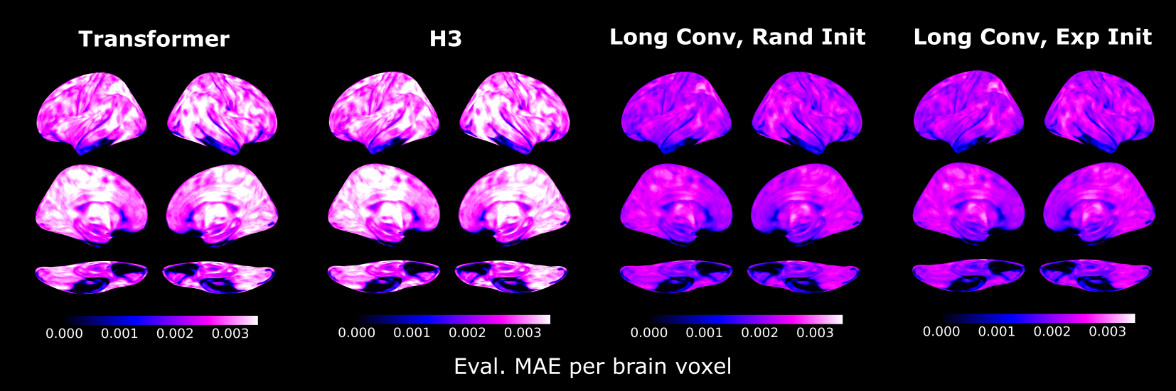
Figure 4: Mean absolute error of pre-trained models in upstream evaluation data for each location of the brain. Brain maps are projected onto the inflated cortical surface of the FsAverage template [22].

Upstream learning:

In line with Thomas et al. [72], we pre-train models $f(\cdot)$ to predict whole-brain activity for the next time point $j$ of an fMRI sequence $X$, using a mean absolute error (MAE) training objective, given the model’s prediction $\hat{X}\in\mathbb{R}^{t\times n}$: MAE $=\frac{1}{n}\sum_{i=1}^{n}|X_{j,i}-\hat{X}_{j,i}|$; $\hat{X}_{t,n}=b_{n}+\sum_{n}f(E^{X})_{t,e}w_{e,n}$; $E^{X}_{t,e}=E^{TR}+E^{pos}+b_{e}+\sum_{n}X_{t,n}w_{n,e}$. Here, $E^{TR}\in\mathbb{R}^{e}$ and $E^{pos}\in\mathbb{R}^{e}$ represent learnable embeddings for each possible time point and position of an input sequence [for details, see 72]. Note that $f(\cdot)$ processes the input in a lower-dimensional representation $E^{X}\in\mathbb{R}^{t\times e}$, where $e=768$, obtained through linear projection.

In line with Thomas et al. [72] and Dao et al. [16], we pre-train a Transformer decoder (based on GPT) with $4$ hidden layers and $12$ attention heads and a H3 model with $4$ hidden layers [with $H=64$ and $m=1$; see 17] in this task. For both models, the sequence of hidden-states outputs of the last model layer are used to determine $\hat{X}$ (scaled to the original input dimension with linear projection). We also pre-train variants of H3 that replace its SSM kernel with long convolutions.

We randomly divide the upstream data, which spans fMRI data from $11,980$ experimental runs of $1,726$ individuals, into distinct training and validation datasets by randomly designating $5\%$ of the fMRI runs as validation data and using the rest of the runs for training. During training, we randomly sample sequences of $100$ time points from the fMRI runs and train models with the ADAM optimizer (with $\beta_{1}=0.9$, $\beta_{2}=0.999$, and $\epsilon=1e^{-8}$ ) for $5,000$ steps at a mini-batch size of $512$ and a learning rate of $5e^{-4}$. We also apply a linear learning rate decay schedule (with a warm-up phase of $10\%$ of the total number of training steps), gradient norm clipping at $1.0$, $L2$-regularisation (weighted by $0.1$), and dropout at a rate of $0.2$ (throughout all models). The adapted H3 variants clearly outperform the other models in accurately predicting brain activity for the next time point of input sequences (Table 9 of the main text). We also find that the pre-trained models exhibit similar evaluation $MAE$ error distributions throughout the brain, with relatively higher errors in the posterior parietal, occipital, and cingulate cortices as well parts of the limbic system (Fig. 4).

References

- Ailon et al. [2021] Ailon, N., Leibovitch, O., and Nair, V. Sparse linear networks with a fixed butterfly structure: theory and practice. In Uncertainty in Artificial Intelligence, pp. 1174–1184. PMLR, 2021.
- Ayinala et al. [2011] Ayinala, M., Brown, M., and Parhi, K. K. Pipelined parallel fft architectures via folding transformation. IEEE Transactions on Very Large Scale Integration (VLSI) Systems, 20(6):1068–1081, 2011.
- Bahn et al. [2009] Bahn, J. H., Yang, J. S., Hu, W.-H., and Bagherzadeh, N. Parallel fft algorithms on network-on-chips. Journal of Circuits, Systems, and Computers, 18(02):255–269, 2009.
- Bailey [1990] Bailey, D. H. FFTs in external or hierarchical memory. The journal of Supercomputing, 4(1):23–35, 1990.
- Barch et al. [2013] Barch, D. M., Burgess, G. C., Harms, M. P., Petersen, S. E., Schlaggar, B. L., Corbetta, M., Glasser, M. F., Curtiss, S., Dixit, S., Feldt, C., et al. Function in the human connectome: task-fmri and individual differences in behavior. Neuroimage, 80:169–189, 2013.
- Bekele [2016] Bekele, A. Cooley-tukey fft algorithms. Advanced algorithms, 2016.
- Brigham [1988] Brigham, E. O. The fast Fourier transform and its applications. Prentice-Hall, Inc., 1988.
- Chen et al. [2021] Chen, B., Dao, T., Liang, K., Yang, J., Song, Z., Rudra, A., and Re, C. Pixelated butterfly: Simple and efficient sparse training for neural network models. In International Conference on Learning Representations, 2021.
- Choromanski et al. [2019] Choromanski, K., Rowland, M., Chen, W., and Weller, A. Unifying orthogonal monte carlo methods. In International Conference on Machine Learning, pp. 1203–1212. PMLR, 2019.
- Chu & George [1999] Chu, E. and George, A. Inside the FFT black box: serial and parallel fast Fourier transform algorithms. CRC press, 1999.
- Cooley & Tukey [1965] Cooley, J. W. and Tukey, J. W. An algorithm for the machine calculation of complex fourier series. Mathematics of Computation, 19(90):297–301, 1965. ISSN 00255718, 10886842. URL http://www.jstor.org/stable/2003354.
- Dadi et al. [2020] Dadi, K., Varoquaux, G., Machlouzarides-Shalit, A., Gorgolewski, K. J., Wassermann, D., Thirion, B., and Mensch, A. Fine-grain atlases of functional modes for fmri analysis. NeuroImage, 221:117126, 2020.
- Dai et al. [2019] Dai, Z., Yang, Z., Yang, Y., Carbonell, J. G., Le, Q., and Salakhutdinov, R. Transformer-xl: Attentive language models beyond a fixed-length context. In Proceedings of the 57th Annual Meeting of the Association for Computational Linguistics, pp. 2978–2988, 2019.
- Dao et al. [2019] Dao, T., Gu, A., Eichhorn, M., Rudra, A., and Ré, C. Learning fast algorithms for linear transforms using butterfly factorizations. In International conference on machine learning, pp. 1517–1527. PMLR, 2019.
- Dao et al. [2022a] Dao, T., Chen, B., Sohoni, N. S., Desai, A., Poli, M., Grogan, J., Liu, A., Rao, A., Rudra, A., and Ré, C. Monarch: Expressive structured matrices for efficient and accurate training. In International Conference on Machine Learning, pp. 4690–4721. PMLR, 2022a.
- Dao et al. [2022b] Dao, T., Fu, D. Y., Ermon, S., Rudra, A., and Ré, C. FlashAttention: Fast and memory-efficient exact attention with IO-awareness. In Advances in Neural Information Processing Systems, 2022b.
- Dao et al. [2022c] Dao, T., Fu, D. Y., Saab, K. K., Thomas, A. W., Rudra, A., and Ré, C. Hungry hungry hippos: Towards language modeling with state space models. arXiv preprint arXiv:2212.14052, 2022c.
- De Sa et al. [2018] De Sa, C., Cu, A., Puttagunta, R., Ré, C., and Rudra, A. A two-pronged progress in structured dense matrix vector multiplication. In Proceedings of the Twenty-Ninth Annual ACM-SIAM Symposium on Discrete Algorithms, pp. 1060–1079. SIAM, 2018.
- Dong et al. [2017] Dong, X., Chen, S., and Pan, S. Learning to prune deep neural networks via layer-wise optimal brain surgeon. Advances in Neural Information Processing Systems, 30, 2017.
- Dosovitskiy et al. [2020] Dosovitskiy, A., Beyer, L., Kolesnikov, A., Weissenborn, D., Zhai, X., Unterthiner, T., Dehghani, M., Minderer, M., Heigold, G., Gelly, S., et al. An image is worth 16x16 words: Transformers for image recognition at scale. In International Conference on Learning Representations, 2020.
- Eidelman & Gohberg [1999] Eidelman, Y. and Gohberg, I. On a new class of structured matrices. Integral Equations and Operator Theory, 34(3):293–324, 1999.
- Fischl [2012] Fischl, B. Freesurfer. Neuroimage, 62(2):774–781, 2012.
- Frankle & Carbin [2018] Frankle, J. and Carbin, M. The lottery ticket hypothesis: Finding sparse, trainable neural networks. arXiv preprint arXiv:1803.03635, 2018.
- Frankle et al. [2019] Frankle, J., Dziugaite, G. K., Roy, D. M., and Carbin, M. Stabilizing the lottery ticket hypothesis. arXiv preprint arXiv:1903.01611, 2019.
- Frankle et al. [2020] Frankle, J., Dziugaite, G. K., Roy, D., and Carbin, M. Linear mode connectivity and the lottery ticket hypothesis. In International Conference on Machine Learning, pp. 3259–3269. PMLR, 2020.
- Gao et al. [2020] Gao, L., Biderman, S., Black, S., Golding, L., Hoppe, T., Foster, C., Phang, J., He, H., Thite, A., Nabeshima, N., et al. The pile: An 800gb dataset of diverse text for language modeling. arXiv preprint arXiv:2101.00027, 2020.
- Goel et al. [2022] Goel, K., Gu, A., Donahue, C., and Ré, C. It’s raw! audio generation with state-space models. arXiv preprint arXiv:2202.09729, 2022.
- Gokaslan et al. [2019] Gokaslan, A., Cohen, V., Pavlick, E., and Tellex, S. Openwebtext corpus, 2019.
- Gu et al. [2020] Gu, A., Dao, T., Ermon, S., Rudra, A., and Ré, C. Hippo: Recurrent memory with optimal polynomial projections. Advances in Neural Information Processing Systems, 33:1474–1487, 2020.
- Gu et al. [2022a] Gu, A., Goel, K., and Ré, C. Efficiently modeling long sequences with structured state spaces. In The International Conference on Learning Representations (ICLR), 2022a.
- Gu et al. [2022b] Gu, A., Gupta, A., Goel, K., and Ré, C. On the parameterization and initialization of diagonal state space models. In Advances in Neural Information Processing Systems, 2022b.
- Gu et al. [2022c] Gu, A., Johnson, I., Timalsina, A., Rudra, A., and Ré, C. How to train your hippo: State space models with generalized orthogonal basis projections. arXiv preprint arXiv:2206.12037, 2022c.
- Guibas et al. [2021] Guibas, J., Mardani, M., Li, Z., Tao, A., Anandkumar, A., and Catanzaro, B. Adaptive fourier neural operators: Efficient token mixers for transformers. arXiv preprint arXiv:2111.13587, 2021.
- Gupta et al. [2022] Gupta, A., Gu, A., and Berant, J. Diagonal state spaces are as effective as structured state spaces. In Advances in Neural Information Processing Systems, 2022.
- Han et al. [2015a] Han, S., Mao, H., and Dally, W. J. Deep compression: Compressing deep neural networks with pruning, trained quantization and huffman coding. arXiv preprint arXiv:1510.00149, 2015a.
- Han et al. [2015b] Han, S., Pool, J., Tran, J., and Dally, W. Learning both weights and connections for efficient neural network. Advances in neural information processing systems, 28, 2015b.
- Hasani et al. [2022] Hasani, R., Lechner, M., Wang, T.-H., Chahine, M., Amini, A., and Rus, D. Liquid structural state-space models. arXiv preprint arXiv:2209.12951, 2022.
- He et al. [2016] He, K., Zhang, X., Ren, S., and Sun, J. Deep residual learning for image recognition. In Proceedings of the IEEE conference on computer vision and pattern recognition, pp. 770–778, 2016.
- Islam & Bertasius [2022] Islam, M. M. and Bertasius, G. Long movie clip classification with state-space video models. arXiv preprint arXiv:2204.01692, 2022.
- Kailath et al. [1979] Kailath, T., Kung, S.-Y., and Morf, M. Displacement ranks of matrices and linear equations. Journal of Mathematical Analysis and Applications, 68(2):395–407, 1979.
- King et al. [2019] King, M., Hernandez-Castillo, C. R., Poldrack, R. A., Ivry, R. B., and Diedrichsen, J. Functional boundaries in the human cerebellum revealed by a multi-domain task battery. Nature neuroscience, 22(8):1371–1378, 2019.
- Krizhevsky et al. [2017] Krizhevsky, A., Sutskever, I., and Hinton, G. E. Imagenet classification with deep convolutional neural networks. Communications of the ACM, 60(6):84–90, 2017.
- LeCun et al. [1998] LeCun, Y., Bottou, L., Bengio, Y., and Haffner, P. Gradient-based learning applied to document recognition. Proceedings of the IEEE, 86(11):2278–2324, 1998.
- Lee-Thorp et al. [2021] Lee-Thorp, J., Ainslie, J., Eckstein, I., and Ontanon, S. Fnet: Mixing tokens with fourier transforms. arXiv preprint arXiv:2105.03824, 2021.
- Li et al. [2021] Li, B., Cheng, S., and Lin, J. tcfft: Accelerating half-precision fft through tensor cores. arXiv preprint arXiv:2104.11471, 2021.
- Li et al. [2022] Li, Y., Cai, T., Zhang, Y., Chen, D., and Dey, D. What makes convolutional models great on long sequence modeling? arXiv preprint arXiv:2210.09298, 2022.
- Liang et al. [2021] Liang, Y., Chongjian, G., Tong, Z., Song, Y., Wang, J., and Xie, P. Evit: Expediting vision transformers via token reorganizations. In International Conference on Learning Representations, 2021.
- Lin et al. [2017] Lin, J., Rao, Y., Lu, J., and Zhou, J. Runtime neural pruning. Advances in neural information processing systems, 30, 2017.
- Lin et al. [2021] Lin, R., Ran, J., Chiu, K. H., Chesi, G., and Wong, N. Deformable butterfly: A highly structured and sparse linear transform. Advances in Neural Information Processing Systems, 34:16145–16157, 2021.
- Ma et al. [2022] Ma, X., Zhou, C., Kong, X., He, J., Gui, L., Neubig, G., May, J., and Zettlemoyer, L. Mega: moving average equipped gated attention. arXiv preprint arXiv:2209.10655, 2022.
- Mehta et al. [2022] Mehta, H., Gupta, A., Cutkosky, A., and Neyshabur, B. Long range language modeling via gated state spaces. arXiv preprint arXiv:2206.13947, 2022.
- Munkhoeva et al. [2018] Munkhoeva, M., Kapushev, Y., Burnaev, E., and Oseledets, I. Quadrature-based features for kernel approximation. Advances in neural information processing systems, 31, 2018.
- Nguyen et al. [2022] Nguyen, E., Goel, K., Gu, A., Downs, G., Shah, P., Dao, T., Baccus, S., and Ré, C. S4nd: Modeling images and videos as multidimensional signals with state spaces. In Advances in Neural Information Processing Systems, 2022.
- NVIDIA [2017] NVIDIA. Nvidia Tesla V100 GPU architecture, 2017.
- NVIDIA [2020] NVIDIA. Nvidia A100 tensor core GPU architecture, 2020.
- NVIDIA [2022a] NVIDIA. cufft v11.7.1 documentation, 2022a. https://docs.nvidia.com/cuda/cufft/index.html.
- NVIDIA [2022b] NVIDIA. Nvidia H100 tensor core GPU architecture, 2022b.
- Olsson et al. [2022] Olsson, C., Elhage, N., Nanda, N., Joseph, N., DasSarma, N., Henighan, T., Mann, B., Askell, A., Bai, Y., Chen, A., Conerly, T., Drain, D., Ganguli, D., Hatfield-Dodds, Z., Hernandez, D., Johnston, S., Jones, A., Kernion, J., Lovitt, L., Ndousse, K., Amodei, D., Brown, T., Clark, J., Kaplan, J., McCandlish, S., and Olah, C. In-context learning and induction heads. Transformer Circuits Thread, 2022. https://transformer-circuits.pub/2022/in-context-learning-and-induction-heads/index.html.
- Oppenheim [1978] Oppenheim, A. V. Applications of digital signal processing. Englewood Cliffs, 1978.
- Oppenheim et al. [2001] Oppenheim, A. V., Buck, J. R., and Schafer, R. W. Discrete-time signal processing. Vol. 2. Upper Saddle River, NJ: Prentice Hall, 2001.
- Parker [1995] Parker, D. Random Butterfly Transformations with Applications in Computational Linear Algebra. CSD (Series). UCLA Computer Science Department, 1995.
- Paszke et al. [2019] Paszke, A., Gross, S., Massa, F., Lerer, A., Bradbury, J., Chanan, G., Killeen, T., Lin, Z., Gimelshein, N., Antiga, L., et al. Pytorch: An imperative style, high-performance deep learning library. Advances in neural information processing systems, 32, 2019.
- Prabhu et al. [2020] Prabhu, A., Farhadi, A., Rastegari, M., et al. Butterfly transform: An efficient fft based neural architecture design. In Proceedings of the IEEE/CVF Conference on Computer Vision and Pattern Recognition, pp. 12024–12033, 2020.
- Romero et al. [2021a] Romero, D. W., Bruintjes, R.-J., Tomczak, J. M., Bekkers, E. J., Hoogendoorn, M., and van Gemert, J. C. Flexconv: Continuous kernel convolutions with differentiable kernel sizes. arXiv preprint arXiv:2110.08059, 2021a.
- Romero et al. [2021b] Romero, D. W., Kuzina, A., Bekkers, E. J., Tomczak, J. M., and Hoogendoorn, M. Ckconv: Continuous kernel convolution for sequential data. In International Conference on Learning Representations, 2021b.
- Sanh et al. [2020] Sanh, V., Wolf, T., and Rush, A. Movement pruning: Adaptive sparsity by fine-tuning. Advances in Neural Information Processing Systems, 33:20378–20389, 2020.
- Sindhwani et al. [2015] Sindhwani, V., Sainath, T., and Kumar, S. Structured transforms for small-footprint deep learning. Advances in Neural Information Processing Systems, 28, 2015.
- Smith et al. [2022] Smith, J. T., Warrington, A., and Linderman, S. W. Simplified state space layers for sequence modeling. arXiv preprint arXiv:2208.04933, 2022.
- Smith et al. [1997] Smith, S. W. et al. The scientist and engineer’s guide to digital signal processing, 1997.
- Tang et al. [2022] Tang, S., Dunnmon, J. A., Qu, L., Saab, K. K., Lee-Messer, C., and Rubin, D. L. Spatiotemporal modeling of multivariate signals with graph neural networks and structured state space models. arXiv preprint arXiv:2211.11176, 2022.
- Tay et al. [2020] Tay, Y., Dehghani, M., Abnar, S., Shen, Y., Bahri, D., Pham, P., Rao, J., Yang, L., Ruder, S., and Metzler, D. Long range arena: A benchmark for efficient transformers. In International Conference on Learning Representations, 2020.
- Thomas et al. [2022] Thomas, A. W., Ré, C., and Poldrack, R. A. Self-supervised learning of brain dynamics from broad neuroimaging data. arXiv preprint arXiv:2206.11417, 2022.
- Trockman & Kolter [2022] Trockman, A. and Kolter, J. Z. Patches are all you need? arXiv preprint arXiv:2201.09792, 2022.
- Varol et al. [2017] Varol, G., Laptev, I., and Schmid, C. Long-term temporal convolutions for action recognition. IEEE transactions on pattern analysis and machine intelligence, 40(6):1510–1517, 2017.
- Vaswani et al. [2017] Vaswani, A., Shazeer, N., Parmar, N., Uszkoreit, J., Jones, L., Gomez, A. N., Kaiser, Ł., and Polosukhin, I. Attention is all you need. Advances in neural information processing systems, 30, 2017.
- Wu et al. [2022] Wu, Y., Rabe, M. N., Hutchins, D., and Szegedy, C. Memorizing transformers. In International Conference on Learning Representations, 2022.
- Zhang et al. [2023] Zhang, M., Saab, K. K., Poli, M., Goel, K., Dao, T., and Ré, C. Effectively modeling time series with simple discrete state spaces. In International Conference on Learning Representations, 2023.
- Zhou et al. [2021] Zhou, H., Zhang, S., Peng, J., Zhang, S., Li, J., Xiong, H., and Zhang, W. Informer: Beyond efficient transformer for long sequence time-series forecasting. In Proceedings of the AAAI conference on artificial intelligence, volume 35, pp. 11106–11115, 2021.
- Zhou et al. [2022] Zhou, L., Poli, M., Xu, W., Massaroli, S., and Ermon, S. Deep latent state space models for time-series generation. arXiv preprint arXiv:2212.12749, 2022.