PerAda: Parameter-Efficient and Generalizable Federated Learning Personalization with Guarantees

Abstract

Personalized Federated Learning (pFL) has emerged as a promising solution to tackle data heterogeneity across clients in FL. However, existing pFL methods either (1) introduce high communication and computation costs or (2) overfit to local data, which can be limited in scope, and are vulnerable to evolved test samples with natural shifts. In this paper, we propose PerAda, a parameter-efficient pFL framework that reduces communication and computational costs and exhibits superior generalization performance, especially under test-time distribution shifts. PerAda reduces the costs by leveraging the power of pretrained models and only updates and communicates a small number of additional parameters from adapters. PerAda has good generalization since it regularizes each client’s personalized adapter with a global adapter, while the global adapter uses knowledge distillation to aggregate generalized information from all clients. Theoretically, we provide generalization bounds to explain why PerAda improves generalization, and we prove its convergence to stationary points under non-convex settings. Empirically, PerAda demonstrates competitive personalized performance (+4.85% on CheXpert) and enables better out-of-distribution generalization (+5.23% on CIFAR-10-C) on different datasets across natural and medical domains compared with baselines, while only updating 12.6% of parameters per model based on the adapter.

1 Introduction

Federated Learning (FL) allows clients to collaboratively train machine learning models without direct access to their data, especially for privacy-sensitive tasks (McMahan et al., 2017). FL was initially designed to train a single global model for all clients. However, such a one-model-fits-all paradigm is not effective when there is client heterogeneity, i.e., the local data are non-IID across clients with heterogeneous features or label distributions (Li et al., 2020b). Personalized Federated Learning (pFL) (Mansour et al., 2020) has emerged as an effective solution to tackle client heterogeneity. In pFL, each client trains a personalized model on its local data to ensure personalized performance, while leveraging the aggregated knowledge from other clients to improve its generalization.

Existing works in pFL commonly use full model personalization, where each client trains a personalized model as well as a copy of the global model from the server for regularization (Li et al., 2021a; T Dinh et al., 2020). However, these methods are parameter-expensive, leading to high computational and communicational costs, which is impractical for clients with limited computation resources and network bandwidth (Kairouz et al., 2021). Later on, partial model personalization alleviates this issue by splitting each client’s one model into personalized parameters and shared parameters, where only the set of shared parameters would be communicated with the server (Pillutla et al., 2022). Nonetheless, these methods tend to overfit more to the local training samples since the set of shared parameters does not encode generalized knowledge well compared to a full global model. This hurts the performance of partially personalized models in real-world FL deployment, where the incoming local test samples are evolving with natural shifts from the local training distribution (Jiang & Lin, 2022).

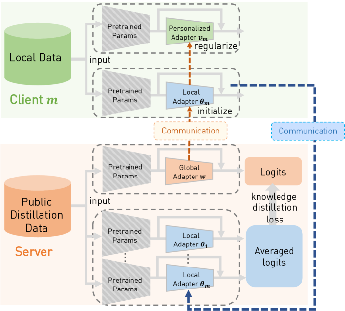
Figure 1: Overview of PerAda. To reduce computation and communication costs, each client only finetunes a personalized adapter and a local adapter based on a pretrained model, and uploads the local adapter. The server aggregates local adapters into a global adapter via knowledge distillation, and sends the global adapter to clients to initialize their local adapters and regularize the training of personalized adapters to improve generalization.

Our Approach. In this work, we aim to design a pFL framework that reduces communication and computation costs while personalizing the model and maintaining its generalization to test-time distribution shifts. We propose PerAda, a parameter-efficient personalized FL framework based on Adapter and Knowledge Distillation (KD). The overview of PerAda is shown in Figure 1.

Each client has a pretrained model, a personalized adapter, and a local adapter, where each adapter consists of a small number of additional parameters planted in the pretrained model with skip connections. At each training round, to reduce the computation and communication costs, PerAda leverages the power of the pretrained model, and only updates the personalized adapter and the local adapter using local data, and sends the local adapter to the server. In this way, it limits the number of trainable parameters and only communicates a smaller number of parameters, the local adapter, instead of the full model to the server.

Then, to improve the generalization, the server aggregates clients’ local adapters (i.e., teachers) via knowledge distillation and trains the global adapter (i.e., student). Specifically, it uses the averaged logits from teachers on an unlabeled public distillation dataset as the pseudo-labels to train the student. This avoids directly averaging clients’ models trained on heterogeneous local data, while enriching the global adapter with the ensemble knowledge from clients’ models and mitigating the model drifts caused by heterogeneity. After that, the server sends the distillated global adapter back to the clients, which is used to initialize the local adapter and regularize the training of the personalized adapter to prevent overfitting and improve the generalization. During the testing phase, each client uses the personalized adapter for inference.

To explain why PerAda is effective at improving generalization, we theoretically derive its generalization bounds under FL covariate (or feature) shift non-IID setting (Marfoq et al., 2022). We are the first to show that the generalization can be enhanced for the global model and personalized models by KD when the distillation error is small, and the distribution of the unlabeled distillation dataset is close to the FL global distribution. We also characterize the role of different components in PerAda on generalization, such as client heterogeneity, pretrained model, and the prediction distance between the global and personalized models.

In addition, we establish convergence guarantees for PerAda in general nonconvex settings to provide theoretical support for practical deep learning model training. The analysis of PerAda is challenging due to the alternative optimization between server distillation training and local client training. We consider a relaxed distillation objective to overcome the challenges. We obtain an ${\mathcal{O}}(1/\sqrt{T})$ convergence rate for the global model and personalized models to stationary points and demonstrate the effects of KD and client heterogeneity on the convergence. These are the first-known results for FL convergence under server distillation.

Empirically, we conduct extensive evaluations on different datasets, including natural and medical images (CIFAR-10, Office-Home, and CheXpert) under both FL covariate-shift and label-shift non-IID settings. We show that PerAda achieves competitive personalized accuracy over state-of-the-art pFL methods with only 12.6% of trainable parameters while obtaining higher generalization, especially when evaluated on out-of-distribution data. We further show that the benefits of PerAda extend to differentially private FL settings and improve the privacy-utility trade-offs compared to full model personalization.

Our contributions are summarized below:

• We propose PerAda, a lightweight pFL framework with personalized adapters that provides personalization while reducing computation/communication costs. We improve the generalization of PerAda with server-side KD.

• We theoretically support the effectiveness of PerAda by generalization bounds and also show an ${\mathcal{O}}(1/\sqrt{T})$ convergence rate for both the global model and personalized models.

• Through extensive experiments we show that PerAda achieves higher personalized performance and better generalization than state-of-the-art pFL methods with smaller computation and communication costs. Moreover, PerAda retains its benifits under differential privacy.

2 Related Work

Full Model Personalization usually requires each client to train a personalized model and a global model, where the global model is used to prevent the personalized model from overfitting to its local data. It includes methods based on meta learning (Fallah et al., 2020), model mixture  (Hanzely & Richtárik, 2020; Deng et al., 2020; Mansour et al., 2020), global reguarlization (Li et al., 2021a), mean regularization (T Dinh et al., 2020; Hanzely & Richtárik, 2020; Hanzely et al., 2020) and clustering (Sattler et al., 2020; Ghosh et al., 2020). However, these methods induce high costs by training two full models in each client and communicating the full model.

Partial Model Personalization trains one model at each client to reduce the costs, which is partitioned into shared parameters and personalized parameters, such as personalized feature extractors (Collins et al., 2021), prediction head (Arivazhagan et al., 2019; Liang et al., 2020; Chen & Chao, 2022), batch normalization (Li et al., 2021b), adapters (Pillutla et al., 2022), and adaptively selected parameters (Sun et al., 2021). Nevertheless, the shared parameters may not learn generalized information well compared to a full global model, so the partially personalized models can have inferior generalization ability.

Knowledge Distillation (KD) in FL. KD is a technique that transfers the knowledge from one or multiple teacher models to a student model (Hinton et al., 2015). Ensemble distillation has been used to tackle data heterogeneity in generic FL, by refining the server model with ensemble knowledge from clients, rather than directly aggregating their model parameters. Specifically, the ensemble predictions from clients’ models on an unlabeled dataset are used to guide the training of the server model, where the unlabeled dataset can be public data (Lin et al., 2020; Chen & Chao, 2020; Li & Wang, 2019) or generated data (Zhang et al., 2022). Another line of work leverages client-side local distillation to transfer global knowledge to local models in generic FL  (Zhu et al., 2021; Lee et al., 2021) or personalized models in pFL (Zhang et al., 2021; Ozkara et al., 2021). To reduce the load for clients, we focus on parameter-efficient adapter-based ensemble distillation in the server with public data to train a better global model, and study its effects on personalized models with novel convergence guarantees and generalization bounds.

3 Preliminaries and Challenges

We consider a typical setting of FL with $M$ clients where each client $m$ has a training dataset ${\mathbb{D}}_{m}=\{\left(x_{m,j},y_{m,j}\right),j\in[n_{m}]\}$ with $n_{m}$ data samples dawn from its local distribution $\mu_{m}$. Let $f(W,x)$ represents a model that outputs the logit vector given input $x$, where $W$ denotes its model parameters. Let the loss function be $\ell(f(W,x),y)$, and the empirical loss on local data ${\mathbb{D}}_{m}$ associated with client $m$ be ${\mathcal{L}}_{m}(W):=\frac{1}{n_{m}}\sum_{j=1}^{n_{m}}\ell\left(f\left(W,x_{m,j}\right),y_{m,j}\right)$.

Personalized FL aims to learn a personalized model for each client to perform well on its local data while preventing overfitting by leveraging the knowledge from other clients. However, achieving the goal is non-trivial due to the following challenges: (1) Communication and computational costs: most full model personalization (Li et al., 2021a; T Dinh et al., 2020), which optimizes ${\min_{W,\{V_{m}\}}\frac{1}{M}\sum_{m=1}^{M}({\mathcal{L}}_{m}(V_{m})+\frac{\lambda}{2}\|V_{m}-W\|^{2})}$, requires twice the memory footprint of the full model at each client by locally updating personalized model $V_{m}\in{\mathbb{R}}^{d}$ and global model $W\in{\mathbb{R}}^{d}$ where $\lambda$ is the $\ell_{2}$ regularization weight controlling the extent of personalization. (2) Limited generalization: partial model personalization (Collins et al., 2021; Liang et al., 2020; Chen & Chao, 2022; Pillutla et al., 2022) is more efficient by training one full model $V_{m}=(u,v_{m})$ at each client and communicating a subset of parameters, where $u\in{\mathbb{R}}^{d_{u}}$ are shared parameters and $v_{m}\in{\mathbb{R}}^{d_{v}}$ are personal parameters: ${\min_{u,\{v_{m}\}}\frac{1}{M}\sum_{m=1}^{M}{\mathcal{L}}_{m}((u,v_{m}))}.$ However, such a partially personalized model can be dominated by personal knowledge with $v_{m}$ and poor at encoding generalized knowledge with the remaining $u$ from FL global distribution, leading to inferior performance under test-time distribution shifts.

4 Method

Here we will introduce the detailed personalized and global objectives of PerAda, as well as its training process.

4.1 Personalized and Global Objectives of PerAda

We address the challenges discussed in Section 3 by proposing PerAda, which improves the efficiency with personalized adapters and enhances their generalization with regularization and KD. Specifically, we train the personalized adapter $\{v_{m}\}$ regularized towards a global adapter $w$ to optimize a personalized objective (Personal Obj), and train a well-generalized $w$ via KD to optimize a global objective (Global Obj) under non-IID data, where we use alternative optimization between client local training of local adapter $\{\theta_{m}\}$ and server KD training of $w$.

Concretely, we improve the efficiency of partial model personalization with a pretrained model and personalized adapters. Here the personalized adapter consists of a small number of additional parameters with skip connections (in Figure 1), which can reduce to the identity function when its parameters are zero (Rebuffi et al., 2017; Zhang et al., 2021). Our personalized adapter is trained with regularization to prevent overfitting, yielding the personal objective:

$$\medmath{\min_{\{v_{m}\}}\frac{1}{M}\sum_{m=1}^{M}P_{m}(v_{m},w),}$$ (Personal Obj)

$$\text{\small with \quad}\medmath{P_{m}(v_{m},w):={\mathcal{L}}_{m}((u,v_{m}))+\frac{\lambda}{2}\|v_{m}-w\|^{2}}$$ (1)

where $u\in{\mathbb{R}}^{d_{u}}$ denotes the fixed pretrained parameters, and $v_{m},w\in{\mathbb{R}}^{d_{a}}$ are personalized adapter and global adapter, respectively, with $d_{a}\ll d_{u}$.

Since the generalization improvement for the personalized adapter $v_{m}$ comes from the $\ell_{2}$ regularization with $w$ in (Personal Obj), it is crucial to enhance the generalization of $w$. Instead of using FedAvg (McMahan et al., 2017) to learn $w$ (i.e., $\min_{w}\frac{1}{M}\sum_{m=1}^{M}{\mathcal{L}}_{m}(w)$) as in regularization-based pFL method (Li et al., 2021a), we leverage server-side ensemble distillation to alleviate model drifts induced by client heterogeneity and enrich the global adapter with ensemble knowledge from clients’ models, yielding the global objective:

$$\medmath{\min_{w,\{\theta_{m}\}}\frac{1}{M}\sum_{m=1}^{M}{\mathcal{L}}_{m}((u,\theta_{m}))+\beta\mathcal{R}_{\mathtt{KD}}(u,\{\theta_{m}\}_{m=1}^{M},w),}$$ (Global Obj)

where $\beta$ is the weight of KD loss and $\theta_{m}\in{\mathbb{R}}^{d_{a}}$ is client $m$’s locally updated global adapter, and we call it as local adapter for distinguishment. The KD loss is defined as:

$$\medmath{\mathcal{R}_{\mathtt{KD}}(u,\{\theta_{m}\}_{m=1}^{M},w):=\sum_{j=1}^{n_{\mathtt{aux}}}\ell_{\mathtt{KD}}(\sum_{m=1}^{M}\frac{f((u,{\theta}_{m}),x_{j})}{M},f((u,w),x_{j})),}$$

i.e., the averaged distillation loss (between the averaged logits of local adapters and logits of the global adapter) on an auxiliary (unlabeled) dataset ${\mathbb{D}}_{\mathtt{aux}}=\{x_{j}\}_{j=1}^{n_{\mathtt{aux}}}$. Here $\ell_{\mathtt{KD}}(a,b)=\mathtt{KL}(\sigma(a/\tau),\sigma(b/\tau))$ is Kullback-Leibler divergence loss where $\sigma$ is softmax function and $\tau$ is tempature (Hinton et al., 2015). Compared to server-side KD in generic FL (Lin et al., 2020; Chen & Chao, 2020; Zhang et al., 2022), we only update adapters instead of full models, which is more efficient for training/communication.

4.2 PerAda Algorithm

Algorithm 1 PerAda with client and server training

1:  Input:$M$ clients, pretrained model $u$, initialized adapters $w^{0}$, $\{v_{m}^{0}\}$, local dataset ${\mathbb{D}}_{m},\forall m\in[M]$, an unlabled dataset ${\mathbb{D}}_{\mathtt{aux}}$

2:  Output: Personalized adapters $v_{1}^{T},\ldots,v_{M}^{T}$  

3:  for communication round $t\in[T]$ do

4:     ${\mathcal{S}}_{t}\leftarrow$ Server samples $C$ clients from $M$ clients

5:     Server sends global adapter ${w}^{t}$ to the selected clients

6:     for client $m\in{\mathcal{S}}_{t}$ do

7:        Client initializes personalized adapter ${v}_{m}^{t,0}$ as ${v}_{m}^{t}$

8:        for step $s\in[S]$ do

9:           /* update personal adapter with batch $\xi_{m}^{t,s}$$\sim$${\mathbb{D}}_{m}$*/

10:           ${v}_{m}^{t,s+1}\leftarrow$ ${v}_{m}^{t,s}-\eta_{p}\nabla\left({\mathcal{L}}_{m}\left((u,{v}_{m}^{t,s}),\xi_{m}^{t,s}\right)+\lambda\left({v}_{m}^{t,s}-{w}^{t}\right)\right)$

11:        end for

12:        Client sets ${v}_{m}^{t+1}\leftarrow{v}_{m}^{t,S}$

13:        Client initializes local adapter ${\theta}_{m}^{t,0}$ as ${w}^{t}$

14:        for step $e\in[E]$ do

15:           /* update local adapter with batch $\xi_{m}^{t,e}$$\sim$${\mathbb{D}}_{m}$*/

16:           ${\theta}_{m}^{t,e+1}\leftarrow{\theta}_{m}^{t,e}-\eta_{l}\nabla{\mathcal{L}}_{m}((u,{\theta}_{m}^{t,e}),\xi_{m}^{t,e})$

17:        end for

18:        Client sends local adapter ${\theta}_{m}^{t+1}\leftarrow{\theta}_{m}^{t,E}$ to server

19:     end for

20:     Server initializes the global adapter $w^{t,0}$ by averaging

21:     $w^{t,0}\leftarrow\sum_{m\in{\mathcal{S}}_{t}}\frac{1}{|{\mathcal{S}}_{t}|}{\theta}_{m}^{t+1}$

22:     for step $r\in[R]$ do

23:        /* update global adapter ${w}^{t+1}$ with batch $\xi^{t,r}$$\sim$${\mathbb{D}}_{\mathtt{aux}}$ */

24:        $w^{t,r+1}\leftarrow$$w^{t,r}-\eta_{g}\beta\nabla_{w}{\mathcal{R}}_{\mathtt{KD}}(u,\{\theta^{t+1}_{m}\}_{m\in{\mathcal{S}}^{t}},w^{t,r},\xi^{t,r})$

25:     end for

26:     Server sets ${w}^{t+1}\leftarrow{w}^{t,R}$

27:  end for

Now we will delve into the details of iteratively optimizing the personalized objective and the global objective introduced in Section 4.1. Algorithm 1 presents our workflow. At each communication round $t\in[T]$, the server selects $C$ clients ${\mathcal{S}}_{t}$ and broadcasts the current global adapter $w^{t}$. To optimize personalized objective, each selected client $m\in{\mathcal{S}}_{t}$ initializes personalized adapter as ${v}_{m}^{t,0}\leftarrow v_{m}^{t}$, and updates it for $S$ steps with learning rate $\eta_{p}$ and mini-batches $\{\xi_{m}^{t,s}\}_{s=0}^{S-1}$ sampled from ${\mathbb{D}}_{m}$ (Line 10). The client sets personalized adapter ${v}_{m}^{t+1}\leftarrow{v}_{m}^{t,S}$ after training. To optimize global objective, each selected client $m$ initializes local adapter as the received global adapter ${\theta}_{m}^{t,0}\leftarrow w^{t}$, and makes local updates for $E$ steps with learning rate $\eta_{l}$ and mini-batches $\{\xi_{m}^{t,e}\}_{e=0}^{E-1}$ sampled from ${\mathbb{D}}_{m}$ (Line 16). Then client $m$ sends the updated local adapter ${\theta}_{m}^{t+1}\leftarrow{\theta}_{m}^{t,E}$ to server. After receiving local adapters, the server first initializes the global adapter by parameter-averaging $w^{t,0}\leftarrow\sum_{m\in{\mathcal{S}}_{t}}\frac{1}{|{\mathcal{S}}_{t}|}{\theta}_{m}^{t+1}$. Then, the server updates global adapter for $R$ steps with learning rate $\eta_{g}$ via knowledge distillation from local adapters (Line  24) where the batches $\{\xi^{t,r}\}_{r=1}^{R}$ are sampled from ${\mathbb{D}}_{\mathtt{aux}}$. The server will send the updated global adapter as $w^{t+1}\leftarrow w^{t,R}$ to clients at the next communication round.

5 Convergence Guarantees of PerAda

In this section, we first introduce a relaxed global objective to theoretically analyze the KD loss, then provide the convergence guarantees for PerAda.

Challenges of Ensemble Distillation and a Relaxed Objective. To the best of our knowledge, there is no convergence guarantee under server-side ensemble distillation (Lin et al., 2020; Chen & Chao, 2020; Li & Wang, 2019; Zhang et al., 2022), and only two works study the convergence under client-side local distillation (Bistritz et al., 2020; Ozkara et al., 2021). This lack of research is likely because: ensemble distillation loss (e.g., $\mathcal{R}_{\mathtt{KD}}$ in (Global Obj)) is calculated upon local models’ averaged logits (ensemble of teachers), so the loss w.r.t each local model (individual teacher) is not directly reflected. However, in standard federated optimization, the “global objective” can usually be “decomposed” into “local objectives” (Li et al., 2020b, a; T Dinh et al., 2020; Fallah et al., 2020), and it is easier to first measure the optimization error on each local objective (i.e., individual teacher) and then derive its implications on the global objective (i.e., ensemble of teachers). Therefore, to make KD loss mathematically tractable for convergence analysis, we focus on its upper bound, i.e., the average of individual distillation loss calculated upon each teacher model. To show this, we introduce a proposition below (see proofs in Appendix A):

Proposition 1.

With $\ell_{\mathtt{KD}}(a,b)=\mathtt{KL}(\sigma(a/\tau),\sigma(b/\tau))$, we have $\ell_{\mathtt{KD}}(\sum_{m=1}^{M}\frac{1}{M}a_{m},b)\leq\frac{1}{M}\sum_{m=1}^{M}\ell_{\mathtt{KD}}(a_{m},b)$.

Let ${\mathcal{R}}(u,\theta_{m},w):=\sum_{j=1}^{n_{\mathtt{aux}}}\ell_{\mathtt{KD}}(f((u,{\theta}_{m}),x_{j}),f((u,w),x_{j}))$, by Proposition 1, we have

$$\medmath{\mathcal{R}_{\mathtt{KD}}(u,\{\theta_{m}\}_{m=1}^{M},w)\leq\frac{1}{M}\sum_{m=1}^{M}{\mathcal{R}}(u,\theta_{m},w)}$$ (2)

Therefore, the (Global Obj) can be relaxed to:

$$\medmath{\min_{w,\{\theta_{m}\}}=\frac{1}{M}\sum_{m=1}^{M}F_{m}(\theta_{m},w)}$$ (Relaxed Global Obj)

$$\medmath{F_{m}(\theta_{m},w):={\mathcal{L}}_{m}\left((u,\theta_{m})\right)+\beta{\mathcal{R}}(u,\theta_{m},w)}$$ (3)

Due to the relaxation in Eq. 2, optimizing (Relaxed Global Obj) also minimizes (Global Obj). We slightly modify the server’s updating rule as below to fit the (Relaxed Global Obj), which is only used in Section 5.2 for theoretical analysis:

(4)

Overview of Analysis. To convey the salient ideas, we consider full client participation (i.e., $|{\mathcal{S}}_{t}|=M$) for convergence analysis following (Reddi et al., 2021; Ozkara et al., 2021); thus, the stochasticity comes from mini-batch samplings during client and server training. The rest of the section is devoted to the convergence analysis w.r.t the (Relaxed Global Obj) and (Personal Obj) for PerAda with the server updating rule (Line 24) replaced by Eq. 4. We start with the assumptions in Section 5.1 and present the convergence guarantees with rates of ${\mathcal{O}}(1/\sqrt{T})$ in Section 5.2. For notation simplicity, we will omit the frozen parameters $u$ and use $w/\theta_{m}/v_{m}$ to represent corresponding models.

5.1 Assumptions

To show convergence, we introduce basic assumptions:

Assumption 1.

(Smoothness) Each ${\mathcal{L}}_{m}(\theta)$ is $L$-Lipschitz smooth, and ${\mathcal{R}}(\theta,w)$ is $L_{R}$-Lipschitz smooth w.r.t $\theta$ and $w$.

Assumption 2.

(Unbiased stochastic gradients and bounded variance) The stochastic gradients are unbiased and their variance is bounded: $\mathbb{E}\left\|\nabla{\mathcal{L}}_{m}\left(\theta,\xi\right)-\nabla{\mathcal{L}}_{m}\left(\theta\right)\right\|^{2}\leq\sigma^{2}$, $\mathbb{E}\left\|\nabla_{w}{\mathcal{R}}(\theta,w,\xi)-\nabla_{w}{\mathcal{R}}(\theta,w)\right\|^{2}\leq\sigma_{R}^{2}$, $\mathbb{E}\left\|\nabla_{\theta}{\mathcal{R}}(\theta,w,\xi)-\nabla_{\theta}{\mathcal{R}}(\theta,w)\right\|^{2}\leq\sigma_{R}^{2}$, $\forall m\in[M]$.

Assumption 3.

(Bounded gradients) The expected squared norm of stochastic gradients is uniformly bounded, i.e., $\mathbb{E}\left\|\nabla{\mathcal{L}}_{m}\left(\theta,\xi\right)\right\|^{2}\leq G^{2}$, $\mathbb{E}\left\|\nabla_{w}{\mathcal{R}}\left(\theta,w,\xi\right)\right\|^{2}\leq G_{R}^{2}$ , $\mathbb{E}\left\|\nabla_{\theta}{\mathcal{R}}\left(\theta,w,\xi\right)\right\|^{2}\leq G_{R}^{2}$. For personalized models, $\mathbb{E}\left\|v_{m}^{t,s}-w^{t}\right\|^{2}\leq G_{\text{reg}}^{2}$ at all clients and all local iterations.

Assumption 4.

(Bounded diversity) The variance of local gradient w.r.t. global gradient is bounded $\left\|\nabla{\mathcal{L}}_{m}({\theta})-\frac{1}{M}\sum_{i=1}^{M}\nabla{\mathcal{L}}_{i}({\theta})\right\|^{2}\leq\gamma_{m}$. At all server iterations, the variance of individual distillation gradient w.r.t. the overall distillation gradient is bounded, $\medmath{\left\|\nabla_{w}{\mathcal{R}}(\theta^{t+1}_{m},w^{t,r})-\frac{1}{M}\sum_{i=1}^{M}\nabla_{w}{\mathcal{R}}(\theta^{t+1}_{i},w^{t,r})\right\|^{2}}$ $\leq\kappa_{m}$. We denote $\bar{\gamma}:=\frac{1}{M}\sum_{m=1}^{M}\gamma_{m}$ and $\bar{\kappa}:=\frac{1}{M}\sum_{m=1}^{M}\kappa_{m}$.

These are common assumptions used when proving the convergence for non-convex FL optimization (Reddi et al., 2021; Li et al., 2020b, 2021a; Ozkara et al., 2021), and we refer the readers to Section A.1 for detailed discussions.

5.2 Convergence Guarantees

We present the main results, and all proofs are relegated to Appendix A due to space constraints.

Theorem 1.

(Convergence of PerAda global model) Let Assumptions 1 to 4 hold, and let $\eta_{g}=\frac{1}{2\beta L_{R}R\sqrt{T}}$, $\eta_{l}=\frac{1}{2(L+\beta L_{R})E\sqrt{T}}$, then for $T\geq 2$, the algorithm satisfies

$$\medmath{\frac{1}{T}\sum_{t=0}^{T-1}\frac{1}{M}\sum_{m=1}^{M}\mathbb{E}\left(\left\|\nabla_{\theta_{m}^{t}}F_{m}(\theta_{m}^{t},w^{t})\right\|^{2}+\left\|\nabla_{w^{t}}F_{m}(\theta_{m}^{t+1},w^{t})\right\|^{2}\right)}$$

$$\medmath{\leq\frac{4\left(L+\beta L_{R}\right)\Delta\overline{F}}{\sqrt{T}-1}+\left(1+\frac{2}{\sqrt{T}-1}\right)\Psi_{1}+\left(\frac{1}{T}+\frac{2}{T(\sqrt{T}-1)}\right)\Psi_{2}}$$

where we define $\medmath{\Delta\overline{F}=\frac{1}{M}\sum_{m=1}^{M}\left(F_{m}(\theta_{m}^{0},w^{0})-F_{m}(\theta_{m}^{T},w^{T})\right)}$, $\medmath{\Psi_{1}}\medmath{=\underbrace{5\bar{\gamma}+3\beta^{2}\bar{\kappa}}_{\text{client heterogeneity}}+\underbrace{9\sigma^{2}+\beta^{2}\sigma_{R}^{2}}_{\text{stochastic gradients}}+\underbrace{5\beta^{2}(G_{R}^{2}-\sigma_{R}^{2})}_{\text{increased distillation loss during local updates}}}$ $\medmath{+\frac{5(L+\beta L_{R})^{2}G_{R}^{2}}{L_{R}^{2}}+\frac{3\beta^{2}L_{R}^{2}G^{2}}{(L+\beta L_{R})^{2}},}$ and $\medmath{\Psi_{2}=\frac{20L^{2}G^{2}}{(L+\beta L_{R})^{2}}+\frac{5L^{2}G_{R}^{2}}{L_{R}^{2}}+\frac{3\beta^{2}G_{R}^{2}}{2}+\frac{3\beta^{2}L_{R}^{2}G^{2}}{2(L+\beta L_{R})^{2}}}$

Remark 1.

We briefly discuss our theoretical analysis. (i) Convergence rate is ${\mathcal{O}}(1/\sqrt{T})$ as it is the dominant term, which matches the rate of the general FL non-convex settings of our interest (Reddi et al., 2021; Karimireddy et al., 2020). (ii) Client heterogeneity is reflected in $\Psi_{1}$, whose effect can be reduced by larger $T$ but would not be completely removed, matching the results in  (Reddi et al., 2021; Ozkara et al., 2021). (iii) Alternative optimization. The error terms with $G^{2},G_{R}^{2}$ in $\Psi_{1},\Psi_{2}$ are due to client drifts with multiple local updates and server distillation updates. The fifth term in $\Psi_{1}$ is due to the increase of distillation loss during clients’ local updates since we do not use local distillation to update local models. To demonstrate the tightness of our analysis for alternative optimization, we remove server KD steps, and Corollary 1 (Section A.1) shows that Theorem 1 directly reduces to FedAvg convergence guarantee. The bound in Corollary 1 is tight as the constant error floor only consists of heterogeneity $\bar{\gamma}$ and stochasticity $\sigma^{2}$. Notably, in the IID setting considered in (Wang & Joshi, 2019), i.e., $\bar{\gamma}=0$, Corollary 1 matches their convergence rates. We further discuss learning rates in Section A.1.

Theorem 2.

(Convergence of PerAda personalized models) Let Assumptions 1 to 4 hold, and let $\eta_{p}=\frac{1}{2(L+\lambda)S\sqrt{T}}$, $\eta_{l}=\frac{1}{2(L+\beta L_{R})E\sqrt{T}}$,$\eta_{g}=\frac{1}{2\zeta\sqrt{T}}$ where $\zeta:=\max\{\beta L_{R}R,\lambda\}$, then for $T\geq 2$, the algorithm satisfies

$$\medmath{\frac{1}{T}\sum_{t=0}^{T-1}\frac{1}{M}\sum_{m=1}^{M}\mathbb{E}\left(\left\|\nabla_{v_{m}^{t}}P_{m}(v_{m}^{t},w^{t})\right\|^{2}+\left\|\nabla_{w^{t}}P_{m}(v_{m}^{t+1},w^{t})\right\|^{2}\right)}$$

$$\medmath{\leq\frac{4\Delta\overline{P}}{\min\{(\zeta\sqrt{T}-\lambda)/\zeta^{2},(\sqrt{T}-1)/(L+\lambda)\}}+\left(1+\frac{2}{\sqrt{T}-1}\right)\sigma^{2}}$$

$$\medmath{\quad\quad+\left(1+\frac{2}{\zeta\sqrt{T}/\lambda-1}\right)\Psi_{3}+\left(\frac{1}{T}+\frac{2}{T(\sqrt{T}-1)}\right)\Psi_{4}}$$

where we define $\medmath{\Delta\overline{P}:=\frac{1}{M}\sum_{m=1}^{M}\left(P_{m}(v_{m}^{0},w^{0})-P_{m}(v_{m}^{T},w^{T})\right)}$, $\medmath{\Psi_{3}=\frac{3\zeta^{2}G^{2}}{(L+\beta L_{R})^{2}}+3\beta^{2}R^{2}G_{R}^{2}+3\lambda^{2}G_{\text{reg}}^{2},\quad\Psi_{4}=\frac{G^{2}+\lambda^{2}G_{\text{reg}}^{2}}{2}}.$

Remark 2.

We also obtain a convergence rate of ${\mathcal{O}}(1/\sqrt{T})$ for personalized models. We show that properly choosing the weight of distillation loss $\beta$ can reduce the error floor $\Psi_{3}$. Increasing regularization strength $\lambda$ does not reduce $\Psi_{3}$ and $\Psi_{4}$, which is because we have not made any assumptions for the distribution of distillation datasets, and current results generally hold for any (out-of-domain) distillation datasets.

6 Generalization Bounds of PerAda

Now we analyze the generalization bounds for PerAda. For notation simplicity, we define $p_{1},\cdots,p_{M}$ as the personalized hypothesis, where each hypothesis $p_{m}\in{\mathcal{P}}_{m}:{\mathcal{X}}\rightarrow[0,1]^{k}$ maps the input $x\in{\mathcal{X}}$ to a probability vector over the $k$ classes (i.e., softmax outputs ${\mathcal{P}}_{m}(x)=\sigma(f((u,v_{m}),x))$). Similarly, we define global hypothesis $g\in{\mathcal{G}}$ and local hypothesis $h_{m}(x)\in\mathcal{H}_{m},\forall m\in[M]$. We also call “hypothesis” as “model” in this section. The local dataset ${\mathbb{D}}_{m}$ of each client $m$ is drawn from the local distribution $\mu_{m}$ and the distillation dataset ${\mathbb{D}}_{\mathtt{aux}}$ of the server is drawn $\mu_{\mathtt{aux}}$. We are interested in the generalization of the global model and personalized models on the FL global distribution $\mu$, by analyzing the effect of local distributions $\{\mu_{m}\}$ and distillation distribution $\mu_{\mathtt{aux}}$. We will present generalization bounds under FL covariate-shift non-IID following  (Marfoq et al., 2022) and defer all proofs to Appendix B.

Global Model. Previous KD-based FL generalization bounds  (Lin et al., 2020; Zhu et al., 2021) simply assume a perfect distillation (i.e., the global model is the ensemble of local models) which neglects the actual distillation error and the choice of distillation distribution. To take them into account, we define the ensemble distillation distance on $n$ points $\{x_{i}\}_{i=1}^{n}$ drawn from the marginal distribution $\mu_{\mathcal{X}}$ as: $\Phi_{\mu,n}(h_{1},\ldots,h_{M};g):=\frac{1}{n}\sum_{i=1}^{n}\|g(x_{i})-\frac{1}{M}\sum_{m=1}^{M}h_{m}(x_{i})\|_{1}$ which measures the output difference between the global model and the ensemble of local models. Here we aim to show $g$ can have good generalization bounds on $\mu$ with KD. Our main idea is to bound error probabilities of $g$ with the expected distillation distances and errors of local models (i.e., teachers), and then bound the errors on $\mu$ with $\mu_{m}$ via prior arts from domain adaptation (Ben-David et al., 2010)

Theorem 3 (Generalization bound of global model).

Let $d_{m}$ be the VC dimension of ${\mathcal{H}}_{m}$, $\operatorname{Rad}_{n}$ be the empirical Rademacher complexity measured on $n$ samples, and the distillation data size and local data size $n_{\mathtt{aux}}=n_{m}=n,\forall m\in[M]$. Then with probability at least $1-\delta$, for every $h_{m}\in{\mathcal{H}}_{m},\forall m\in[M]$ and $g\in{\mathcal{G}}$, we have

$$\medmath{\operatorname{Pr}_{(x,y)\sim\mu}\left[\underset{y^{\prime}}{\arg\max}g(x)_{y^{\prime}}\neq y\right]\leq 2\mathbb{E}_{(x,y)\sim\mu}(1-g(x)_{y})}$$

$$\medmath{\leq\frac{1}{M}\sum_{m=1}^{M}\left[2\underbrace{\mathbb{E}_{(x,y)\sim\mu_{m}}(1-h_{m}(x)_{y})}_{\text{local model's population risk on local distribution}}\right]}$$

$$\medmath{+\frac{1}{M}\sum_{m=1}^{M}\left(\underbrace{{\hat{d}}_{{\mathcal{H}}\Delta{\mathcal{H}}}({\mathbb{D}}_{m},{\mathbb{D}})}_{\text{distribution divergence}}+\lambda_{m}+8\sqrt{\frac{2d_{m}\log(2n)+\log(4M/\delta)}{n}}\right)}$$

$$\medmath{+2\underbrace{\Phi_{\mu_{\mathtt{aux}},n}(h_{1},\ldots,h_{M};g)}_{\text{ensemble distillation distance}}+4\underbrace{\mathbb{TV}(\mu,\mu_{\mathtt{aux}})}_{\text{TV divergence}}+6\sqrt{\frac{\log(4/\delta)}{2n}}}$$

$$\medmath{+\widetilde{\mathcal{O}}\left({k^{3/2}}\left[\max_{j}\left(\frac{1}{M}\sum_{m=1}^{M}\operatorname{Rad}_{n}(\mathcal{H}_{m}|_{j})\right)+\max_{j}\operatorname{Rad}_{n}(\mathcal{G}|_{j})\right]\right)}$$

where $\medmath{\lambda_{m}=\varepsilon_{\mu_{m}}(h^{*})+\varepsilon_{\mu}(h^{*}),h^{*}:=\arg\min_{h\in{\mathcal{H}}}\varepsilon_{\mu_{m}}(h)+\varepsilon_{\mu}(h)}$.

Remark 3.

We briefly discuss key implications of Theorem 3. (i) Quality of local models. The first term shows that reducing the population risk of local models w.r.t local distributions $\mu_{m}$ improves the generalization of the global model. We verify in Section 7.1 that a more powerful pretrained model, which results in higher quality local models, leads to better generalization. (ii) Ensemble distillation. $\Phi_{\mu_{\mathtt{aux}},n}$ captures the distillation error measured on the distillation dataset ${\mathbb{D}}_{\mathtt{aux}}$ as minimized in Line 24. When $\mu_{\mathtt{aux}}=\mu$, e.g., using public validation data as the distillation dataset, KD improves the generalization of $g$ during training by directly minimizing $\Phi_{\mu_{\mathtt{aux}},n}$. The smaller the distillation distance, the better the generalization. When $\mu_{\mathtt{aux}}\neq\mu$, KD on $\mu_{\mathtt{aux}}$ decreases $\Phi_{\mu_{\mathtt{aux}},n}$ while causing additional generalization gap measured by TV divergence $\mathbb{TV}(\mu_{\mathtt{aux}},\mu)$. Compared to without KD, using a distillation dataset from a domain close to $\mu$ with small $\mathbb{TV}(\mu_{\mathtt{aux}},\mu)$ and reducing $\Phi_{\mu_{\mathtt{aux}},n}$ during KD can also improve the generalization (e.g., $\Phi_{\mu_{\mathtt{aux}},n}+2\mathbb{TV}(\mu_{\mathtt{aux}},\mu)$ evaluated on KD-trained-models is smaller than $\Phi_{\mu,n}$ evaluated on non-KD-trained-models). We empirically verify it in Section 7.1. (iii) Sample complexity. More empirical samples $n$ improve the generalization. We further discuss client heterogeneity ${\hat{d}}_{{\mathcal{H}}\Delta{\mathcal{H}}}({\mathbb{D}}_{m},{\mathbb{D}})$ and number of classes $k$ in Section B.1.

Table 1: Parameter-efficiency and averaged test accuracy across clients’ personalized models. PerAda achieves higher personalized performance and generalization with a smallest $\#$ of trainable parameters. Underline/bold fonts highlight the best baseline/our approach.

Algorithm

Personalized Params

$\#$ Trained Params

$\#$ Comm. Params

CIFAR-10

Office-Home

CheXpert

$\operatorname{Local-test}$

$\operatorname{Global-test}$

CIFAR-10.1

CIFAR-10-C

$\operatorname{Local-test}$

$\operatorname{Global-test}$

$\operatorname{Local-test}$

$\operatorname{Global-test}$

Standalone

Full model

11.18$M$

0$M$

$85.94$${}\pm{}$

$8.82$

$29.77$${}\pm{}$

$8.09$

$25.82$${}\pm{}$

$6.27$

$26.67$${}\pm{}$

$7.07$

$81.64$${}\pm{}$

$6.08$

$59.15$${}\pm{}$

$3.32$

$65.06$${}\pm{}$

$1.88$

$65.45$${}\pm{}$

$2.3$

MTL

Full model

11.18$M$

11.18$M$

$86.24$${}\pm{}$

$8.45$

$29.46$${}\pm{}$

$8.33$

$25.64$${}\pm{}$

$6.42$

$26.4$${}\pm{}$

$7.29$

$81.82$${}\pm{}$

$5.53$

$59.25$${}\pm{}$

$2.84$

$65.15$${}\pm{}$

$1.95$

$65.48$${}\pm{}$

$2.3$

pFedMe

Full model

22.36$M$

11.18$M$

$90.73$${}\pm{}$

$4.67$

$45.06$${}\pm{}$

$8.65$

$36.51$${}\pm{}$

$7.2$

$37.65$${}\pm{}$

$7.6$

$80.21$${}\pm{}$

$5.32$

$75.69$${}\pm{}$

$0.69$

$65.07$${}\pm{}$

$1.2$

$64.86$${}\pm{}$

$1.22$

APFL

Full model

22.36$M$

11.18$M$

90.74${}\pm{}$

$4.75$

$43.92$${}\pm{}$

$9.18$

$35.83$${}\pm{}$

$7.5$

$36.51$${}\pm{}$

$7.94$

$81.24$${}\pm{}$

$4.51$

76.98${}\pm{}$

$1.39$

$68.98$${}\pm{}$

$1.04$

$68.96$${}\pm{}$

$1.1$

Ditto

Full model

22.36$M$

11.18$M$

$90.21$${}\pm{}$

$4.61$

53.82${}\pm{}$

$6.35$

42.72${}\pm{}$

$5.68$

44.32${}\pm{}$

$5.73$

$81.77$${}\pm{}$

$4.31$

$75.66$${}\pm{}$

$1.01$

$68.79$${}\pm{}$

$1.4$

$68.86$${}\pm{}$

$1.22$

FedBN

Batch norm.

11.18$M$

11.17$M$

$90.37$${}\pm{}$

$5.19$

$43.18$${}\pm{}$

$8.67$

$35.01$${}\pm{}$

$7.24$

$36.29$${}\pm{}$

$7.43$

$81.86$${}\pm{}$

$5.13$

$74.26$${}\pm{}$

$0.52$

$68.74$${}\pm{}$

$1.17$

$68.83$${}\pm{}$

$1.08$

FedAlt

Input layer

11.18$M$

6.45$M$

$87.07$${}\pm{}$

$6.54$

$32.23$${}\pm{}$

$8.23$

$27.49$${}\pm{}$

$6.41$

$28.51$${}\pm{}$

$7.11$

$81.07$${}\pm{}$

$5.59$

$65.85$${}\pm{}$

$0.9$

$67.63$${}\pm{}$

$1.18$

$67.74$${}\pm{}$

$1.1$

FedSim

Input layer

11.18$M$

6.45$M$

$87.93$${}\pm{}$

$6.25$

$33.07$${}\pm{}$

$8.16$

$28.21$${}\pm{}$

$6.41$

$29.15$${}\pm{}$

$7.16$

$82.45$${}\pm{}$

$5.03$

$67.66$${}\pm{}$

$0.82$

$67.49$${}\pm{}$

$1.32$

$67.54$${}\pm{}$

$1.24$

LG-FedAvg

Feat. extractor

11.18$M$

0.005$M$

$86.7$${}\pm{}$

$8.01$

$29.96$${}\pm{}$

$8$

$25.97$${}\pm{}$

$6.21$

$26.83$${}\pm{}$

$6.95$

$82.04$${}\pm{}$

$5.96$

$63.57$${}\pm{}$

$2.32$

$65.78$${}\pm{}$

$1.62$

$66.23$${}\pm{}$

$1.75$

FedRep

Output layer

11.18$M$

11.17$M$

$87.76$${}\pm{}$

$6.46$

$35.19$${}\pm{}$

$6.97$

$30.15$${}\pm{}$

$5.89$

$30.68$${}\pm{}$

$6.31$

$79.05$${}\pm{}$

$5.88$

$74.17$${}\pm{}$

$2.02$

$66.66$${}\pm{}$

$1.82$

$66.52$${}\pm{}$

$1.47$

FedAlt

Output layer

11.18$M$

11.17$M$

$89.68$${}\pm{}$

$5.4$

$40.68$${}\pm{}$

$7.3$

$33.61$${}\pm{}$

$6.12$

$34.3$${}\pm{}$

$6.5$

83.24${}\pm{}$

$3.96$

$70.62$${}\pm{}$

$1.46$

$68.27$${}\pm{}$

$1.3$

$68.36$${}\pm{}$

$1.31$

FedSim

Output layer

11.18$M$

11.17$M$

$89.75$${}\pm{}$

$5.51$

$41.98$${}\pm{}$

$7.66$

$34.21$${}\pm{}$

$6.22$

$35.31$${}\pm{}$

$6.79$

$82.91$${}\pm{}$

$4.46$

$72.34$${}\pm{}$

$0.51$

$68.22$${}\pm{}$

$1.34$

$68.12$${}\pm{}$

$1.24$

FedAlt

Adapter

12.59$M$

11.18$M$

$87.26$${}\pm{}$

$7.78$

$31.51$${}\pm{}$

$8.55$

$27.38$${}\pm{}$

$6.65$

$27.77$${}\pm{}$

$7.19$

$81.41$${}\pm{}$

$6.5$

$57.88$${}\pm{}$

$3.57$

72.13${}\pm{}$

$1.34$

74.67${}\pm{}$

$1.57$

FedSim

Adapter

12.59$M$

11.18$M$

$87.76$${}\pm{}$

$7.57$

$31.97$${}\pm{}$

$7.44$

$27.76$${}\pm{}$

$5.78$

$28.1$${}\pm{}$

$6.46$

$82.14$${}\pm{}$

$5.46$

$58.62$${}\pm{}$

$3.24$

$71.75$${}\pm{}$

$1.4$

$74.09$${}\pm{}$

$1.55$

PerAda-

Adapter

2.82$M$

1.41$M$

$91.27$${}\pm{}$

$5.15$

$53.81$${}\pm{}$

$6.27$

$42.5$${}\pm{}$

$5.06$

$44.45$${}\pm{}$

$5.48$

$83.31$${}\pm{}$

$5.54$

$76.55$${}\pm{}$

$2.47$

$76.77$${}\pm{}$

$2.24$

$77.59$${}\pm{}$

$2.18$

PerAda

Adapter

2.82$M$

1.41$M$

91.82${}\pm{}$

$4.43$

59.05${}\pm{}$

$5.24$

47.25${}\pm{}$

$4.48$

48.53${}\pm{}$

$4.74$

83.58${}\pm{}$

$4.74$

77.2${}\pm{}$

$1.63$

76.98${}\pm{}$

$3.87$

77.88${}\pm{}$

$1.55$

Personalized Models. We show that personalized model $p_{m}$ can generalize well on $\mu$ if global model $g$ generalizes well on $\mu$ and $p_{m}$ has small prediction distance with $g$.

Theorem 4 (Generalization bound of personalized model).

With probability at least $1-\delta$, for every $p_{m}\in{\mathcal{P}}_{m},\forall m\in[M]$, and for every $g\in{\mathcal{G}}$, we have

$$\medmath{\operatorname{Pr}_{(x,y)\sim\mu}\left[\underset{y^{\prime}}{\arg\max}p_{m}(x)_{y^{\prime}}\neq y\right]\leq{2\mathbb{E}_{(x,y)\sim\mu}(1-g(x)_{y})}}$$

$$\medmath{+2\frac{1}{n}\sum_{i=1}^{n}\min\left\{1,\|p_{m}(x)-g(x)\|_{1}\right\}+6\sqrt{\frac{\log(2/\delta)}{2n}}}$$

$$\medmath{+\widetilde{\mathcal{O}}\left({k^{3/2}}\left[\max_{j}\operatorname{Rad}_{n}(\mathcal{P}|_{j})+\max_{j}\operatorname{Rad}_{n}(\mathcal{G}|_{j})\right]\right)}$$

Remark 4.

The first term is the population risk of $g$ on $\mu$, which has been upper bounded by Theorem 3. Therefore the personalized model can inherit the generalization ability of global model discussed in Remark 3. The second term is the prediction difference between $g$ and personalized models. In Section 7.1, we empirically show that moderately increasing the regularization strength $\lambda$ in (Personal Obj) could improve the generalization of $p_{m}$, by reducing such prediction distance.

7 Experiments

We empirically compare PerAda to existing pFL methods. We defer the details of experiments and hyperparameter as well as the additional experimental results to Appendix C.

Data and Model. We use CIFAR-10 (Krizhevsky et al., 2009), Office-Home (Venkateswara et al., 2017), and medical image data CheXpert (Irvin et al., 2019). We simulate pFL setting for (1) label Non-IID using Dirichlet distribution $\operatorname{Dir}(\alpha)$ (Hsu et al., 2019) with $\alpha=0.1/0.3$ on CIFAR-10/CheXpert, creating different local data size and label distributions for $M$ clients; and (2) feature Non-IID on Office-Home by distributing the data from 4 domains (Art, Clipart, Product, and Real Word) to 4 clients respectively (Sun et al., 2021). We use $M=20$ for CIFAR-10/CheXpert, and sample 40% clients at every round following (Chen & Chao, 2022; Lin et al., 2020), and use full client participation for Office-Home following (Sun et al., 2021). For all datasets, we train every FL algorithm on a ResNet-18 model pretrained on ImageNet-1K (Russakovsky et al., 2015). For PerAda, we use out-of-domain distillation dataset CIFAR-100 for CIFAR-10, and use CIFAR-10 for Office-Home/CheXpert.

Baselines. We evaluate full model pFL methods Ditto (Li et al., 2021a), APFL (Deng et al., 2020), MTL (Smith et al., 2017), pFedMe (T Dinh et al., 2020), and partial model pFL methods LG-FedAvg (Liang et al., 2020), FedRep (Collins et al., 2021), FedSim (Pillutla et al., 2022), FedAlt (Pillutla et al., 2022), as well as our PerAda^-, which is PerAda without KD (w/o Line 24).

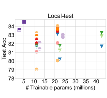
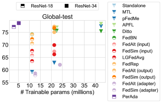
Figure 2: Accuracy of pFL on ResNet-18/34 with Office-Home. PerAda achieves the highest personalized performance and generalization with the smallest # trainable parameters.

Evaluation Metrics. We report the averaged test accuracy (pFL accuracy) and standard deviation over all clients’ personalized models. For CheXpert, we report the AUC score since it is a multi-label classification task. We evaluate pFL accuracy mainly under two metrics: $\operatorname{Local-test}$ (i.e., clients’ corresponding local test data) and $\operatorname{Global-test}$ (i.e., the union of clients’ local test data), to study the personalized performance and generalization (against label or covariate shifts), respectively. In addition, for CIFAR-10, we evaluate pFL generalization against distribution shifts on CIFAR-10.1 (Recht et al., 2018) and common image corruptions (e.g. Blur, Gaussian Noise) on CIFAR-10-C (Hendrycks & Dietterich, 2019).

7.1 Evaluation Results

PerAda is parameter-efficient. The ResNet-18 model consists of 11.18 million (M) parameters, and the adapter has 1.41M (12.6%) parameters. Table 1 reports each client’s # trainable parameters and # communicated parameters to the server. We see that PerAda is most parameter-efficient by locally training two adapters and communicating one adapter. Most full model pFL requires training two full models (pFedMe, APFL, Ditto), and sends one full model to the server. Partial model pFL requires training one full model and communicating its shared parameter. Note that adapter-based partial model pFL in FedAlt and FedSim are more expensive than PerAda because they still need to train both a personalized adapter plus a shared full model (12.59M), and communicate the full model. Additional comparison under the ResNet-34 model architecture shows similar conclusions in Figure 2.

PerAda achieves competitive personalized performance and better generalization than baselines. Table 1 shows that even with the smallest number of trainable parameters, PerAda achieves the comparable personalized performance (+1.08%, 0.34%, 4.85% on CIFAR-10, Office-Home, CheXpert) and better generalization (+5.23%, 4.53%, 4.21%, 0.22%, 3.21% on CIFAR-10, CIFAR-10.1, CIFAR-10-C, Office-Home, CheXpert). Specifically, (a) PerAda^- already achieves favorable performance compared to the best baseline, which shows that the plug-in module adapter can adapt the pretrained model to FL data distributions, and personalized adapter can successfully encode both local knowledge (with local empirical risk) and generalized knowledge (with regularization). (b) PerAda outperforms PerAda^-, which shows that KD improves the generalization of personalized models (Theorem 4). To verify that such improvement is due to improved global adapter (Theorem 3), we compare the performance of the global model of PerAda to the global model in pFL methods (pFedMe, APFL, Ditto) and generic FL methods (FedProx (Li et al., 2020a), FedDyn (Acar et al., 2020), FedDF (Lin et al., 2020)) on CIFAR-10. Additional results in Table 8 (Appendix D) shows that the generalization of PerAda global model outperforms baselines, and KD indeed improves our global model.

Existing partial model pFL can have poor generalization to out-of-distribution shifts. Table 1 shows that although existing partial model pFL methods have favorable personalized performance on CIFAR-10 and sometimes outperform full model pFL on Office-Home and CheXpert by personalizing the right “component”, they can be significantly worse than full model pFL to test-time distribution shifts. We attribute this to the smaller number of shared parameters to learn global information and the fact that personalized parameters can predominately encode local information for the model. PerAda circumvents such issue by KD and regularization, which enforce personalized adapter to learn both local and global information.

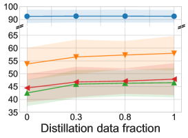
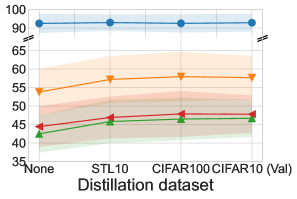
Figure 3: Effect of KD on PerAda evaluated on CIFAR-10. More distillation steps and data lead to better generalization, and the out-of-domain distillation datasets (STL-10, CIFAR-100) achieve similar performance as CIFAR-10 validation data.

Adapter-based personalization methods are generally effective on CheXpert. In Table 1, we observe that adapter-based personalization including FedAlt, FedSim, PerAda are especially effective on the X-ray data CheXpert. This conclusion holds under different FL data heterogeneity degrees ($\operatorname{Dir}(0.3)$ and $\operatorname{Dir}(1)$) in Table 7 (Appendix D). It indicates that when adapting to FL domains that have a large domain gap for ImageNet pre-trained models, e.g., medical domains, adapter personalization may be preferable to input/output/batch norm personalization.

Effects of KD. We use CIFAR-100 as the distillation dataset on CIFAR-10, and Figure 3 shows that more distillation steps and distillation data samples are better for pFL generalization. These results echo our theoretical analysis in Theorem 3 that smaller KD optimization error $\Phi_{\mu_{\mathtt{aux}},n_{\mathtt{aux}}}$ and a larger number of samples can tighten the generalization bounds. We also evaluate different distillation datasets, and Figure 3 shows that out-of-domain datasets (STL-10, CIFAR100) can improve generalization compared to the one without KD (None) by a margin, and achieve comparable performance compared to in-domain CIFAR10 validation data. The flexibility of choosing distillation datasets makes it practical for the server to leverage public data for KD.

Another potential way to improve generalization is by moderately increasing regularization strength $\lambda$ for less personalization. However, additional results in Figure 5 (Appendix D) show that an overly large $\lambda$ degrades the personalized performance, which matches the observation for $\ell_{2}$ regularization-based pFL methods in (Pillutla et al., 2022). Notably, KD does not have such a negative impact on personalized performance (in Figure 3).

Table 2: Utility under DP guarantees on CIFAR-10 with ViT-S/16-224 model. PerAda achieves high personalized accuracy under the same DP guarantee.

Algorithm	$\epsilon=\infty$	$\epsilon=5.99\pm 3.03$	$\epsilon=3.7\pm 2.12$	$\epsilon=1.81\pm 1.12$
Ditto	98.59 $\pm$ 1.63	76.76 $\pm$ 24.14	76.75 $\pm$ 24.13	76.67 $\pm$ 24.12
PerAda-	97.69 $\pm$ 1.79	77.49 $\pm$ 21.21	77.32 $\pm$ 21.16	76.68 $\pm$ 21
PerAda	98.08 $\pm$ 1.28	80.33$\pm$ 20.76	79.79 $\pm$20.45	77.83$\pm$ 19.58

Effects of pretrained models. Starting personalization from a pretrained model, such as FedAvg model (Pillutla et al., 2022; Marfoq et al., 2022), is common in pFL, so we report the results with FedAvg pretrained model (on FL data from scratch) for all methods on CIFAR-10. Figure 4 (Appendix D) shows that PerAda also achieves comparable personalized performance and higher generalization than baselines with FedAvg pretrained model. Moreover, Theorem 3 shows that high-quality local models (enabled by good pretrained model) can further improve generalization. Here, we use ImageNet as an example of high-quality pretrained models, which leads to even higher personalized performance and generalization for PerAda. We defer more discussions to Appendix D.

Utility under differential privacy guarantees. To further protect local data privacy, we train our method under sample-level $(\epsilon,\delta)$ -differential privacy (DP) (Dwork et al., 2014) on CIFAR-10 with a ViT-S/16-224 model. Following (Liu et al., 2022), we consider full client participation and perform local training with DP-SGD (Abadi et al., 2016) for both personalized models and the global model (see experimental details in Appendix C); We set $\delta=10^{-5}$ and report averaged $\epsilon$ across all clients and averaged pFL accuracy under $\operatorname{Local-test}$. Table 2 shows that (1) PerAda^- (without KD) retains higher utility than full model personalization Ditto under reasonable privacy guarantees due to a smaller number of trainable parameters and the whole model is less impacted by DP noise. (2) KD with unlabeled public data in PerAda can further improve the utility without consuming additional privacy budgets.

8 Conclusion

We propose a pFL framework PerAda based on adapter and knowledge distillation. We provide convergence and generalization guarantees and show that PerAda reduces computation and communication costs and achieves higher personalized performance and generalization.

Appendix

The Appendix is organized as follows:

• Appendix A provides the convergence analysis of PerAda and the full proofs for Theorem 1 and Theorem 2.

• Appendix B provides the generalization analysis of PerAda and the full proofs for Theorem 3 and Theorem 4.

• Appendix C provides detailed setup and hyperparameters for experiments.

• Appendix D provides additional experiment results.

Appendix A Convergence Analysis

In this section, we present the discussions and analysis for our convergence guarantees. The outline of this section is as follows:

• Section A.1 provides more discussions on our assumption as well as Theorem 1, and then present Corollary 1.

• Section A.2 provides the proofs for relaxed distillation loss in Proposition 1.

• Section A.3 provides the proofs for the global model convergence guarantee in Theorem 1.

• Section A.4 provides the proofs for the personalized model convergence guarantee in Theorem 2.

A.1 Additional Discussions and Theoretical Results

More Discussions for Our Assumptions.

Assumptions 1, 2, 3 are standard in nonconvex optimization (Reddi et al., 2016) and FL optimization (Reddi et al., 2021; Li et al., 2020b, 2021a) literature. In 3, $\left\|v_{m}^{t,s}-w^{t}\right\|^{2}$ is part of $\left\|\nabla_{{v}_{m}^{t,s}}P_{m}({v}_{m}^{t,s},w^{t},\xi_{m}^{t,s})\right\|^{2}$, so by combining $G_{\text{reg}}^{2}$ with the bound for the gradient of local loss $G^{2}$ (i.e., bound of $\left\|\nabla{\mathcal{L}}_{m}\left(v_{m}^{t,s},\xi\right)\right\|^{2}$), it is equivalent to directly assume $\mathbb{E}\left\|\nabla_{{v}_{m}^{t,s}}P_{m}({v}_{m}^{t,s},w^{t},\xi_{m}^{t,s})\right\|^{2}$ is bounded as used in (Li et al., 2021a). In 4, the bounded diversity for local gradients is widely used in FL to characterize the client data heterogeneity. We assume the bounded diversity for each client $\gamma_{m}$ so that the averaged diversity is bounded by $\gamma$. Previous work usually assumes the averaged bounded diversity $\gamma$ directly (Reddi et al., 2021; T Dinh et al., 2020; Fallah et al., 2020; Pillutla et al., 2022). Our assumption for $\gamma_{m}$ is used to tackle the client’s local drifts during the alternative updating, while previous work does not consider such alternative optimization between server and clients in FL. Similarly, we assume bounded diversity for the distillation gradients, which is similar to the assumption in  (Ozkara et al., 2021), which focuses on local distillation (rather than server-side distillation). Note that  (Reddi et al., 2021; Li et al., 2021a) also assume both bounded gradients and bounded diversity.

More Discussions for Theorem 1.

In Theorem 1, we choose learning rates $\eta_{l},\eta_{g}$ of $1/\sqrt{T}$ following  (Reddi et al., 2021; Ozkara et al., 2021). This is because the client drifts introduced by local updates and server distillation updates do not vanish as $T\rightarrow\infty$ when $\eta_{l},\eta_{g}$ are constant.

Connection to FedAvg Convergence.

We present the Corollary 1 below and discuss its implications in FL:

Corollary 1.

(Connection to the convergence of FedAvg global model) Without server KD, by setting $\eta_{g}=\eta_{l}=\frac{1}{2LE\sqrt{T}}$, $\beta=0,G_{R}^{2}=0$, and let Assumptions 1 to 4 hold, Theorem 1 can be reduced to FedAvg convergence:

$$\medmath{\frac{1}{T}\sum_{t=0}^{T-1}\frac{1}{M}\sum_{m=1}^{M}\mathbb{E}\left\|\nabla_{w^{t}}F_{m}(w^{t})\right\|^{2}\leq\frac{4L\Delta\overline{F}}{\sqrt{T}-1}+}\medmath{\left(1+\frac{2}{\sqrt{T}-1}\right)\left(5\bar{\gamma}+9\sigma^{2}\right)+\left(\frac{1}{T}+\frac{2}{T(\sqrt{T}-1)}\right)20G^{2}}.$$

Remark 5.

Corollary 1 verifies the tightness of the bounds in Theorem 1 because there are no terms related to server optimization, and the constant error floor only consists of client heterogeneity $\bar{\gamma}$ and local gradients stochasticity $\sigma^{2}$. We also note that in the i.i.d setting considered in (Wang & Joshi, 2019), i.e., $\bar{\gamma}=0$, we match their convergence rates.

A.2 Proof for Proposition 1

Here we provide the proof for Proposition 1, which are used to derive our relaxed objective of knowledge distillation.

Proof for Proposition 1.

Due to the convexity of Kullback-Leibler divergence $\mathtt{KL}(\cdot,\cdot)$ and softmax function $\sigma(\cdot)$, for any $\Lambda\in[0,1]$, we have

$$\mathtt{KL}\left(\left(\sigma\left(\Lambda a_{1}+(1-\Lambda)a_{2}\right)/\tau\right),\sigma(b/\tau)\right)$$

$$\leq\mathtt{KL}(\Lambda\sigma(a_{1}/\tau)+(1-\Lambda)\sigma(a_{2}/\tau),\sigma(b/\tau))$$

$$\leq\Lambda\mathtt{KL}(\sigma(a_{1}/\tau),\sigma(b/\tau))+(1-\Lambda)\mathtt{KL}(\sigma(a_{2}/\tau),\sigma(b/\tau)).$$

Therefore, $\ell_{\mathtt{KD}}(a,b)$ is a convex function. Then, since $\sum_{m=1}^{M}\frac{1}{M}=1$, by interatively using the convex property for $M$ times for $a_{1},\cdots,a_{M}$ respectively, we have $\ell_{\mathtt{KD}}(\sum_{m=1}^{M}\frac{1}{M}a_{m},b)\leq\frac{1}{M}\sum_{m=1}^{M}\ell_{\mathtt{KD}}(a_{m},b)$. ∎

A.3 Proofs for the Global Model Convergence Guarantee in Theorem 1

For notation simplicity, we define the parameter-averaged model as $\bar{\theta}^{t+1}=\frac{1}{M}\sum_{m=1}^{M}{\theta}_{m}^{t+1}$, which is used to initialize the server global model at round $t$ before the KD training.

Based on the update rules, we define $g^{t}$ and $g_{m}^{t}$ as

$$g^{t}:=-\frac{1}{\eta_{g}}(w^{t+1}-\bar{\theta}^{t+1})=\beta\sum_{r=0}^{R-1}\frac{1}{M}\sum_{m=1}^{M}\nabla_{w}{\mathcal{R}}(\theta^{t+1}_{m},w^{t,r},\xi^{t,r}),\quad g_{m}^{t}:=-\frac{1}{\eta_{l}}(\theta_{m}^{t+1}-w^{t})=\sum_{e=0}^{E-1}\nabla{\mathcal{L}}_{m}({\theta}_{m}^{t,e},\xi_{m}^{t,e})$$ (5)

According to server update rule $w^{t+1}-w^{t}=\bar{\theta}^{t+1}-w^{t}-\eta_{g}g^{t}$. Note that $\bar{\theta}^{t+1}-w^{t}=\frac{1}{M}\sum_{m=1}^{M}{\theta}_{m}^{t+1}-w^{t}=-\frac{1}{M}\sum_{m=1}^{M}\eta_{l}g_{m}^{t}$ based on Eq. 5. Then we define,

$$\delta_{w}^{t}:=\frac{1}{M}\sum_{m=1}^{M}\frac{\eta_{l}}{\eta_{g}}g_{m}^{t}+g^{t},\text{\quad which indicates $w^{t+1}-w^{t}=-\eta_{g}\delta_{w}^{t}$}$$ (6)

According to client update rule $\theta_{m}^{t+1}-\theta_{m}^{t}=(w^{t}-\eta_{l}g_{m}^{t})-(w^{t-1}-\eta_{l}g_{m}^{t-1})$. Note that $w^{t}-w^{t-1}=-\eta_{l}\frac{1}{M}\sum_{m=1}^{M}g_{m}^{t}-\eta_{g}g^{t}$ based on Eq. 5. Then we define,

$$\delta_{\theta_{m}}^{t}:=\frac{\eta_{g}}{\eta_{l}}g^{t-1}+\frac{1}{M}\sum_{i=1}^{M}g_{i}^{t-1}-g_{m}^{t-1}+g_{m}^{t},\text{\quad which indicates $\theta_{m}^{t+1}-\theta_{m}^{t}=-\eta_{l}\delta_{\theta_{m}}^{t}$}$$ (7)

Proof Outline

The goal is to bound the gradients of local models and global model w.r.t the (Global Obj), which is used to show that the trained models can converge to the stationary points:

$$\frac{1}{T}\sum_{t=0}^{T-1}\frac{1}{M}\sum_{m=1}^{M}\left(\left\|\nabla_{\theta_{m}^{t}}F_{m}(\theta_{m}^{t},w^{t})\right\|^{2}+\left\|\nabla_{w^{t}}F_{m}(\theta_{m}^{t+1},w^{t})\right\|^{2}\right)$$

We use the smoothness assumptions 1 for $w$ and $\theta_{m}$ at each round $t$:

$$F_{m}(\theta_{m}^{t+1},w^{t})\leq F_{m}(\theta_{m}^{t},w^{t})+\left\langle\nabla_{\theta_{m}^{t}}F_{m}(\theta_{m}^{t},w^{t}),\theta_{m}^{t+1}-\theta_{m}^{t}\right\rangle+\frac{L+\beta L_{R}}{2}\left\|\theta_{m}^{t+1}-\theta_{m}^{t}\right\|^{2},$$ (8)

$$F_{m}(\theta_{m}^{t+1},w^{t+1})\leq F_{m}(\theta_{m}^{t+1},w^{t})+\left\langle\nabla_{w^{t}}F_{m}(\theta_{m}^{t+1},w^{t}),w^{t+1}-w^{t}\right\rangle+\frac{\beta L_{R}}{2}\left\|w^{t+1}-w^{t}\right\|^{2},$$ (9)

Note that by combining the above two inequalities together, $F_{m}(\theta_{m}^{t+1},w^{t})$ can be canceled out. Thus we can derive the upper bound for gradient w.r.t $w$ (i.e., $\left\|\nabla_{w^{t}}F_{m}(\theta_{m}^{t+1},w^{t})\right\|^{2}$) and gradient w.r.t $\theta$ (i.e., $\left\|\nabla_{\theta_{m}^{t}}F_{m}(\theta_{m}^{t},w^{t})\right\|^{2}$) with $F_{m}(\theta_{m}^{t},w^{t})-F_{m}(\theta_{m}^{t+1},w^{t+1})$. Iterating over $T$ rounds and $M$ clients, we can derive the final bound.

Challenges

The challenges of convergence analysis include:

(1) Alternative optimization. The server optimization of $w$ will be influenced by the drift of client optimization of $\theta_{m}$, as shown in Eq. 6 (i.e., additional deviation with the term $\frac{1}{M}\sum_{m=1}^{M}\frac{\eta_{l}}{\eta_{g}}g_{m}^{t}$). Moreover, client optimization is also influenced by the drift of server optimization, as shown in Eq. 7 (i.e., additional deviation with the terms $\frac{\eta_{g}}{\eta_{l}}g^{t-1}+\frac{1}{M}\sum_{i=1}^{M}g_{i}^{t-1}-g_{m}^{t-1}$).

(2) The actual local update of $\theta$ does not consider the distillation loss. Therefore, $m$-th client’s local update does not minimize the corresponding objective $F_{m}$, which includes both local empirical risk and the distillation loss, bringing the error floor.

Before we start, we introduce a useful existing result by Jensen’s inequality in Proposition 2:

Proposition 2.

For any vector $x_{i}\in\mathbb{R}^{d},i=1,\ldots,M$, by Jensen’s inequality, we have

$$\left\|\sum_{i=1}^{M}x_{i}\right\|^{2}\leq M\sum_{i=1}^{M}\left\|x_{i}\right\|^{2}$$

A.3.1 Analysis of Client Update for $\theta_{m}$.

We present the key lemma for the gradients w.r.t $\theta_{m}$ here and then delve into its proofs.

Lemma 1 (Bounding the gradients w.r.t $\theta_{m}$).

Let Assumptions 1 to 4 hold, then we have,

$$\left(\frac{\eta_{l}E}{2}-\left(L+\beta L_{R}\right)\eta_{l}^{2}E^{2}\right)\left\|\nabla_{\theta_{m}^{t}}F_{m}(\theta_{m}^{t},w^{t})\right\|^{2}\leq F_{m}(\theta_{m}^{t},w^{t})-F_{m}(\theta_{m}^{t+1},w^{t})$$

$$\quad+\left(\frac{\eta_{l}}{2E}+\left(L+\beta L_{R}\right)\eta_{l}^{2}\right)\left(5\frac{\eta_{g}^{2}}{\eta_{l}^{2}}\beta^{2}R^{2}G_{R}^{2}+80E^{4}L^{2}G^{2}\eta_{l}^{2}+20E^{2}L^{2}\beta^{2}R^{2}G_{R}^{2}\eta_{g}^{2}+5E^{2}\beta^{2}(G_{R}^{2}-\sigma_{R}^{2})+5E^{2}\gamma_{m}+9E^{2}\sigma^{2}\right)$$ (10)

Proof.

By the smoothness of $F_{m}(\theta,w)$ w.r.t to $\theta$ in 1, we have

$$F_{m}(\theta_{m}^{t+1},w^{t})\leq F_{m}(\theta_{m}^{t},w^{t})+\left\langle\nabla_{\theta_{m}^{t}}F_{m}(\theta_{m}^{t},w^{t}),\theta_{m}^{t+1}-\theta_{m}^{t}\right\rangle+\frac{L+\beta L_{R}}{2}\left\|\theta_{m}^{t+1}-\theta_{m}^{t}\right\|^{2}$$ (11)

$$\left\langle\nabla_{\theta_{m}^{t}}F_{m}(\theta_{m}^{t},w^{t}),\theta_{m}^{t+1}-\theta_{m}^{t}\right\rangle+\frac{L+\beta L_{R}}{2}\left\|\theta_{m}^{t+1}-\theta_{m}^{t}\right\|^{2}$$

$$=-\eta_{l}\left\langle\nabla_{\theta_{m}^{t}}F_{m}(\theta_{m}^{t},w^{t}),\delta_{\theta_{m}}^{t}\right\rangle+\frac{L+\beta L_{R}}{2}\eta_{l}^{2}\left\|\delta_{\theta_{m}}^{t}\right\|^{2}$$ (By Eq. 7)

$$=-\eta_{l}\left\langle\nabla_{\theta_{m}^{t}}F_{m}(\theta_{m}^{t},w^{t}),\delta_{\theta_{m}}^{t}-E\nabla_{\theta_{m}^{t}}F_{m}(\theta_{m}^{t},w^{t})+E\nabla_{\theta_{m}^{t}}F_{m}(\theta_{m}^{t},w^{t})\right\rangle$$

$$\quad\quad+\frac{L+\beta L_{R}}{2}\eta_{l}^{2}\left\|\delta_{\theta_{m}}^{t}-E\nabla_{\theta_{m}^{t}}F_{m}(\theta_{m}^{t},w^{t})+E\nabla_{\theta_{m}^{t}}F_{m}(\theta_{m}^{t},w^{t})\right\|^{2}$$

$$\leq-\eta_{l}\left\langle\nabla_{\theta_{m}^{t}}F_{m}(\theta_{m}^{t},w^{t}),\delta_{\theta_{m}}^{t}-E\nabla_{\theta_{m}^{t}}F_{m}(\theta_{m}^{t},w^{t})\right\rangle-\eta_{l}E\|\nabla_{\theta_{m}^{t}}F_{m}(\theta_{m}^{t},w^{t})\|^{2}$$

$$\quad\quad+\left(L+\beta L_{R}\right)\eta_{l}^{2}\left\|\delta_{\theta_{m}}^{t}-E\nabla_{\theta_{m}^{t}}F_{m}(\theta_{m}^{t},w^{t})\right\|^{2}+\left(L+\beta L_{R}\right)\eta_{l}^{2}E^{2}\left\|\nabla_{\theta_{m}^{t}}F_{m}(\theta_{m}^{t},w^{t})\right\|^{2}$$ (By Proposition 2)

$$\leq\frac{\eta_{l}E}{2}\left\|\nabla_{\theta_{m}^{t}}F_{m}(\theta_{m}^{t},w^{t})\right\|^{2}+\frac{\eta_{l}}{2E}\left\|\delta_{\theta_{m}}^{t}-E\nabla_{\theta_{m}^{t}}F_{m}(\theta_{m}^{t},w^{t})\right\|^{2}-\eta_{l}E\|\nabla_{\theta_{m}^{t}}F_{m}(\theta_{m}^{t},w^{t})\|^{2}$$ (By Cauchy-Schwarz inequality and AM-GM inequality)

$$\quad\quad+\left(L+\beta L_{R}\right)\eta_{l}^{2}\left\|\delta_{\theta_{m}}^{t}-E\nabla_{\theta_{m}^{t}}F_{m}(\theta_{m}^{t},w^{t})\right\|^{2}+\left(L+\beta L_{R}\right)\eta_{l}^{2}E^{2}\left\|\nabla_{\theta_{m}^{t}}F_{m}(\theta_{m}^{t},w^{t})\right\|^{2}$$

$$=-\left(\frac{\eta_{l}E}{2}-\left(L+\beta L_{R}\right)\eta_{l}^{2}E^{2}\right)\left\|\nabla_{\theta_{m}^{t}}F_{m}(\theta_{m}^{t},w^{t})\right\|^{2}+\left(\frac{\eta_{l}}{2E}+\left(L+\beta L_{R}\right)\eta_{l}^{2}\right)\left\|\delta_{\theta_{m}}^{t}-E\nabla_{\theta_{m}^{t}}F_{m}(\theta_{m}^{t},w^{t})\right\|^{2}$$

Then we bound $\left\|\delta_{\theta_{m}}^{t}-E\nabla_{\theta_{m}^{t}}F_{m}(\theta_{m}^{t},w^{t})\right\|^{2}$ as below

$$\mathbb{E}\left\|\delta_{\theta_{m}}^{t}-E\nabla_{\theta_{m}^{t}}F_{m}(\theta_{m}^{t},w^{t})\right\|^{2}$$

$$=\mathbb{E}\left\|\frac{\eta_{g}}{\eta_{l}}g^{t-1}+\frac{1}{M}\sum_{i=1}^{M}g_{i}^{t-1}-g_{m}^{t-1}+g_{m}^{t}-E\nabla_{\theta_{m}^{t}}F_{m}(\theta_{m}^{t},w^{t})\right\|^{2}$$

$$=\mathbb{E}\left\|\frac{\eta_{g}}{\eta_{l}}g^{t-1}+\frac{1}{M}\sum_{i=1}^{M}\sum_{e=0}^{E-1}\nabla{\mathcal{L}}_{i}({\theta}_{i}^{t-1,e},\xi_{m}^{t-1,e})-\sum_{e=0}^{E-1}\nabla{\mathcal{L}}_{m}({\theta}_{m}^{t-1,e},\xi_{m}^{t-1,e})+\sum_{e=0}^{E-1}\nabla{\mathcal{L}}_{m}({\theta}_{m}^{t,e},\xi_{m}^{t,e})\right.$$

$$\quad\quad\left.-E\left(\nabla{\mathcal{L}}_{m}(\theta_{m}^{t})+\beta\nabla_{\theta_{m}^{t}}{\mathcal{R}}(\theta_{m}^{t},w^{t})\right)\right\|^{2}$$ (By definitions in Eq. 5 and Eq. 3)

$$\leq\mathbb{E}\left\|\frac{\eta_{g}}{\eta_{l}}g^{t-1}-E\beta\nabla_{\theta_{m}^{t}}{\mathcal{R}}(\theta_{m}^{t},w^{t})+\frac{1}{M}\sum_{i=1}^{M}\sum_{e=0}^{E-1}\nabla{\mathcal{L}}_{i}({\theta}_{i}^{t-1,e})-\sum_{e=0}^{E-1}\nabla{\mathcal{L}}_{m}({\theta}_{m}^{t-1,e})+\sum_{e=0}^{E-1}\nabla{\mathcal{L}}_{m}({\theta}_{m}^{t,e})-E\nabla{\mathcal{L}}_{m}(\theta_{m}^{t})\right\|^{2}+9E^{2}\sigma^{2} \mathbb{E}\|X\|^{2}=\|\mathbb{E}X\|^{2}+\mathbb{E}\|X-\mathbb{E}X\|^{2}$$ (by , Proposition 2, and 2)

$$=\mathbb{E}\left\|\frac{\eta_{g}}{\eta_{l}}g^{t-1}-E\beta\nabla_{\theta_{m}^{t}}{\mathcal{R}}(\theta_{m}^{t},w^{t})+\sum_{e=0}^{E-1}\frac{1}{M}\sum_{i=1}^{M}\nabla{\mathcal{L}}_{i}({\theta}_{i}^{t-1,e})-\sum_{e=0}^{E-1}\frac{1}{M}\sum_{i=1}^{M}\nabla{\mathcal{L}}_{i}({\theta}_{m}^{t-1,e})+\sum_{e=0}^{E-1}\frac{1}{M}\sum_{i=1}^{M}\nabla{\mathcal{L}}_{i}({\theta}_{m}^{t-1,e})\right.$$

$$\quad\quad\left.-\sum_{e=0}^{E-1}\nabla{\mathcal{L}}_{m}({\theta}_{m}^{t-1,e})+\sum_{e=0}^{E-1}\left(\nabla{\mathcal{L}}_{m}({\theta}_{m}^{t,e})-\nabla{\mathcal{L}}_{m}(\theta_{m}^{t}))\right)\right\|^{2}+9E^{2}\sigma^{2}$$

$$=\mathbb{E}\left\|\frac{\eta_{g}}{\eta_{l}}g^{t-1}-E\beta\nabla_{\theta_{m}^{t}}{\mathcal{R}}(\theta_{m}^{t},w^{t})+\sum_{e=0}^{E-1}\frac{1}{M}\sum_{i=1}^{M}\left(\nabla{\mathcal{L}}_{i}({\theta}_{i}^{t-1,e})-\nabla{\mathcal{L}}_{i}({\theta}_{m}^{t-1,e})\right)+\sum_{e=0}^{E-1}\left(\frac{1}{M}\sum_{i=1}^{M}\nabla{\mathcal{L}}_{i}({\theta}_{m}^{t-1,e})-\nabla{\mathcal{L}}_{m}({\theta}_{m}^{t-1,e})\right)\right.$$

$$\quad\quad\left.+\sum_{e=0}^{E-1}\left(\nabla{\mathcal{L}}_{m}({\theta}_{m}^{t,e})-\nabla{\mathcal{L}}_{m}(\theta_{m}^{t})\right)\right\|^{2}+9E^{2}\sigma^{2}$$

$$\leq 5\mathbb{E}\left\|\frac{\eta_{g}}{\eta_{l}}g^{t-1}\right\|^{2}+5\mathbb{E}\left\|E\beta\nabla_{\theta_{m}^{t}}{\mathcal{R}}(\theta_{m}^{t},w^{t})\right\|^{2}+5\left\|\sum_{e=0}^{E-1}\frac{1}{M}\sum_{i=1}^{M}\left(\nabla{\mathcal{L}}_{i}({\theta}_{i}^{t-1,e})-\nabla{\mathcal{L}}_{i}({\theta}_{m}^{t-1,e})\right)\right\|^{2}+$$

$$\quad\quad 5\mathbb{E}\left\|\sum_{e=0}^{E-1}\left(\frac{1}{M}\sum_{i=1}^{M}\nabla{\mathcal{L}}_{i}({\theta}_{m}^{t-1,e})-\nabla{\mathcal{L}}_{m}({\theta}_{m}^{t-1,e})\right)\right\|^{2}+5\mathbb{E}\left\|\sum_{e=0}^{E-1}\left(\nabla{\mathcal{L}}_{m}({\theta}_{m}^{t,e})-\nabla{\mathcal{L}}_{m}(\theta_{m}^{t})\right)\right\|^{2}+9E^{2}\sigma^{2}$$ (By Proposition 2)

$$\leq 5\frac{\eta_{g}^{2}}{\eta_{l}^{2}}\mathbb{E}\left\|g^{t-1}\right\|^{2}+5E^{2}\beta^{2}\mathbb{E}\left\|\nabla_{\theta_{m}^{t}}{\mathcal{R}}(\theta_{m}^{t},w^{t})\right\|^{2}+5EL^{2}\sum_{e=0}^{E-1}\frac{1}{M}\sum_{i=1}^{M}\mathbb{E}\left\|{\theta}_{i}^{t-1,e}-{\theta}_{m}^{t-1,e}\right\|^{2}+5E^{2}\gamma_{m}$$

$$\quad\quad+5EL^{2}\sum_{e=0}^{E-1}\mathbb{E}\left\|{\theta}_{m}^{t,e}-\theta_{m}^{t}\right\|^{2}+9E^{2}\sigma^{2}$$ (By 4 and 1)

We bound each term in the RHS as below. For $\mathbb{E}\left\|g^{t-1}\right\|^{2}$, we have,

$$\mathbb{E}\left\|g^{t-1}\right\|^{2}=\mathbb{E}\left\|\beta\sum_{r=0}^{R-1}\frac{1}{M}\sum_{m=1}^{M}\nabla_{w}{\mathcal{R}}(\theta^{t}_{m},w^{t-1,r},\xi^{t-1,r})\right\|^{2} \leq\beta^{2}R\sum_{r=0}^{R-1}\frac{1}{M}\sum_{m=1}^{M}\mathbb{E}\left\|\nabla_{w}{\mathcal{R}}(\theta^{t}_{m},w^{t-1,r},\xi^{t-1,r})\right\|^{2}$$ (by Proposition 2)

$$\leq\beta^{2}R^{2}G_{R}^{2}$$ (by 3)

For $\left\|\nabla_{\theta_{m}^{t}}{\mathcal{R}}(\theta_{m}^{t},w^{t})\right\|^{2}$, we have,

$$\left\|\nabla_{\theta_{m}^{t}}{\mathcal{R}}(\theta_{m}^{t},w^{t})\right\|^{2} =\mathbb{E}\left\|\nabla_{\theta_{m}^{t}}{\mathcal{R}}(\theta_{m}^{t},w^{t},\xi_{m}^{t})\right\|^{2}-\mathbb{E}\left\|\nabla_{\theta_{m}^{t}}{\mathcal{R}}(\theta_{m}^{t},w^{t})-\nabla_{\theta_{m}^{t}}{\mathcal{R}}(\theta_{m}^{t},w^{t},\xi_{m}^{t})\right\|^{2} \|\mathbb{E}X\|^{2}=\mathbb{E}\|X\|^{2}-\mathbb{E}\|X-\mathbb{E}X\|^{2}$$ (by )

$$\leq G_{R}^{2}-\sigma_{R}^{2}$$ (by 3 and 2)

For $\mathbb{E}\left\|{\theta}_{i}^{t-1,e}-{\theta}_{m}^{t-1,e}\right\|^{2}$, we have,

$$\mathbb{E}\left\|{\theta}_{i}^{t-1,e}-{\theta}_{m}^{t-1,e}\right\|^{2} =\left\|w^{t-1}-\eta_{l}\sum_{j=0}^{e-1}\nabla{\mathcal{L}}_{i}({\theta}_{i}^{t-1,j},\xi_{i}^{t-1,j})-w^{t-1}+\eta_{l}\sum_{j=0}^{e-1}\nabla{\mathcal{L}}_{m}({\theta}_{m}^{t-1,j},\xi_{m}^{t-1,j})\right\|^{2}$$

$$=\eta_{l}^{2}\mathbb{E}\left\|\sum_{j=0}^{e-1}\left(\nabla{\mathcal{L}}_{i}({\theta}_{i}^{t-1,j},\xi_{i}^{t-1,j})-\nabla{\mathcal{L}}_{m}({\theta}_{m}^{t-1,j},\xi_{m}^{t-1,j})\right)\right\|^{2}$$

$$\leq\eta_{l}^{2}e\sum_{j=0}^{e-1}\mathbb{E}\left\|\nabla{\mathcal{L}}_{i}({\theta}_{i}^{t-1,j},\xi_{i}^{t-1,j})-\nabla{\mathcal{L}}_{m}({\theta}_{m}^{t-1,j},\xi_{m}^{t-1,j})\right\|^{2}$$ (by Proposition 2)

$$\leq\eta_{l}^{2}e\sum_{j=0}^{e-1}\left(2\mathbb{E}\left\|\nabla{\mathcal{L}}_{i}({\theta}_{i}^{t-1,j},\xi_{i}^{t-1,j})\right\|^{2}+2\mathbb{E}\left\|\nabla{\mathcal{L}}_{m}({\theta}_{m}^{t-1,j},\xi_{m}^{t-1,j})\right\|^{2}\right)$$ (by Proposition 2)

$$\leq 4\eta_{l}^{2}e^{2}G^{2}$$ (by 3)

For $\mathbb{E}\left\|{\theta}_{m}^{t,e}-{\theta}_{m}^{t}\right\|^{2}$, we have,

$$\mathbb{E}\left\|{\theta}_{m}^{t,e}-{\theta}_{m}^{t}\right\|^{2} =\mathbb{E}\left\|({\theta}_{m}^{t,e}-w^{t})-({\theta}_{m}^{t}-w^{t-1})+(w^{t}-w^{t-1})\right\|^{2}$$

$$=\mathbb{E}\left\|({\theta}_{m}^{t-1,E}-w^{t})-({\theta}_{m}^{t}-w^{t-1})+(w^{t}-\bar{\theta}^{t})+(\bar{\theta}^{t}-w^{t-1})\right\|^{2}$$

$$=\mathbb{E}\left\|-\eta_{l}\sum_{j=0}^{e-1}\nabla{\mathcal{L}}_{m}({\theta}_{m}^{t,j},\xi_{m}^{t,j})+\eta_{l}\sum_{j=0}^{E-1}\nabla{\mathcal{L}}_{m}({\theta}_{m}^{t-1,j},\xi_{m}^{t-1,j})\right.$$

$$\quad\quad\left.-\eta_{g}\beta\sum_{r=0}^{R-1}\frac{1}{M}\sum_{i=1}^{M}\nabla_{w^{t-1,r}}{\mathcal{R}}({\theta}_{i}^{t,e},w^{t-1,r},\xi^{t-1,r})-\eta_{l}\frac{1}{M}\sum_{i=1}^{M}\sum_{j=0}^{E-1}\nabla{\mathcal{L}}_{i}({\theta}_{i}^{t-1,j},\xi_{i}^{t-1,j})\right\|^{2}$$

$$\leq 4\mathbb{E}\left\|\eta_{l}\sum_{j=0}^{e-1}\nabla{\mathcal{L}}_{m}({\theta}_{m}^{t,j},\xi_{m}^{t,j})\right\|^{2}+4\mathbb{E}\left\|\eta_{l}\sum_{j=0}^{E-1}\nabla{\mathcal{L}}_{m}({\theta}_{m}^{t-1,j},\xi_{m}^{t-1,j})\right\|^{2}$$

$$\quad\quad+4\mathbb{E}\left\|\eta_{g}\beta\sum_{r=0}^{R-1}\frac{1}{M}\sum_{i=1}^{M}\nabla_{w^{t-1,r}}{\mathcal{R}}({\theta}_{i}^{t,e},w^{t-1,r},\xi^{t-1,r})\right\|^{2}+4\mathbb{E}\left\|\eta_{l}\frac{1}{M}\sum_{i=1}^{M}\sum_{j=0}^{E-1}\nabla{\mathcal{L}}_{i}({\theta}_{i}^{t-1,j},\xi_{i}^{t-1,j})\right\|^{2}$$ (by Proposition 2)

$$\leq 4\eta_{l}^{2}e\sum_{j=0}^{e-1}\mathbb{E}\left\|\nabla{\mathcal{L}}_{m}({\theta}_{m}^{t,j},\xi_{m}^{t,j})\right\|^{2}+4\eta_{l}^{2}E\sum_{j=0}^{E-1}\mathbb{E}\left\|\nabla{\mathcal{L}}_{m}({\theta}_{m}^{t-1,j},\xi_{m}^{t-1,j})\right\|^{2}$$

$$\quad\quad+4\eta_{g}^{2}\beta^{2}R\sum_{r=0}^{R-1}\frac{1}{M}\sum_{i=1}^{M}\mathbb{E}\left\|\eta_{g}\beta\nabla_{w^{t-1,r}}{\mathcal{R}}({\theta}_{i}^{t,e},w^{t-1,r},\xi^{t-1,r})\right\|^{2}+4\eta_{l}^{2}E\sum_{j=0}^{E-1}\frac{1}{M}\sum_{i=1}^{M}\mathbb{E}\left\|\nabla{\mathcal{L}}_{i}({\theta}_{i}^{t-1,j},\xi_{i}^{t-1,j})\right\|^{2}$$ (by Proposition 2)

$$\leq 4\eta_{l}^{2}e^{2}G^{2}+4\eta_{l}^{2}E^{2}G^{2}+4\eta_{g}^{2}\beta^{2}R^{2}G_{R}^{2}+4\eta_{l}^{2}E^{2}G^{2}$$ (By 3)

$$\leq 4\eta_{l}^{2}e^{2}G^{2}+8\eta_{l}^{2}E^{2}G^{2}+4\eta_{g}^{2}\beta^{2}R^{2}G_{R}^{2}$$

Combining the above results together, we have

$$\left\|\delta_{\theta_{m}}^{t}-E\nabla_{\theta_{m}^{t}}F_{m}(\theta_{m}^{t},w^{t})\right\|^{2}$$

$$\leq 5\frac{\eta_{g}^{2}}{\eta_{l}^{2}}\mathbb{E}\left\|g^{t-1}\right\|^{2}+5E^{2}\beta^{2}\mathbb{E}\left\|\nabla_{\theta_{m}^{t}}{\mathcal{R}}(\theta_{m}^{t},w^{t})\right\|^{2}+5EL^{2}\sum_{e=0}^{E-1}\frac{1}{M}\sum_{i=1}^{M}\mathbb{E}\left\|{\theta}_{i}^{t-1,e}-{\theta}_{m}^{t-1,e}\right\|^{2}+5E^{2}\gamma_{m}$$

$$\quad\quad+5EL^{2}\sum_{e=0}^{E-1}\mathbb{E}\left\|{\theta}_{m}^{t,e}-\theta_{m}^{t}\right\|^{2}+9E^{2}\sigma^{2}$$

$$\leq 5\frac{\eta_{g}^{2}}{\eta_{l}^{2}}\beta^{2}R^{2}G_{R}^{2}+5E^{2}\beta^{2}(G_{R}^{2}-\sigma_{R}^{2})+20EL^{2}\sum_{e=0}^{E-1}\eta_{l}^{2}e^{2}G^{2}+5E^{2}\gamma_{m}$$

$$\quad\quad+5EL^{2}\sum_{e=0}^{E-1}\left(4\eta_{l}^{2}e^{2}G^{2}+8\eta_{l}^{2}E^{2}G^{2}+4\eta_{g}^{2}\beta^{2}R^{2}G_{R}^{2}\right)+9E^{2}\sigma^{2}$$

$$\leq 5\frac{\eta_{g}^{2}}{\eta_{l}^{2}}\beta^{2}R^{2}G_{R}^{2}+80E^{4}L^{2}G^{2}\eta_{l}^{2}+20E^{2}L^{2}\beta^{2}R^{2}G_{R}^{2}\eta_{g}^{2}+5E^{2}\beta^{2}(G_{R}^{2}-\sigma_{R}^{2})+5E^{2}\gamma_{m}+9E^{2}\sigma^{2} e\leq E$$ (By )

∎

A.3.2 Analysis of Server Update for $w$.

We present the below key lemma for the gradients w.r.t $w$ and then give its proofs.

Lemma 2 (Bounding the gradients w.r.t $w$).

Let Assumptions 1 to 4 hold, then we have,

$$\left(\frac{\eta_{g}R}{2}-\beta L_{R}\eta_{g}^{2}R^{2}\right)\left\|\nabla_{w^{t}}F_{m}(\theta_{m}^{t+1},w^{t})\right\|^{2}\leq\quad F_{m}(\theta_{m}^{t+1},w^{t})-F_{m}(\theta_{m}^{t+1},w^{t+1})$$

$$\quad+\left(\frac{\eta_{g}}{2R}+\beta L_{R}\eta_{g}^{2}\right)\left(3\frac{\eta_{l}^{2}}{\eta_{g}^{2}}E^{2}G^{2}+6\beta^{4}L_{R}^{2}R^{4}G_{R}^{2}\eta_{g}^{2}+6\beta^{2}L_{R}^{2}R^{2}E^{2}G^{2}\eta_{l}^{2}+3\beta^{2}R^{2}\kappa_{m}+R^{2}\beta^{2}\sigma_{R}^{2}\right)$$ (12)

Proof.

By the smoothness of $F_{m}(\theta,w)$ w.r.t to $w$ in 1, we have

$$F_{m}(\theta_{m}^{t+1},w^{t+1})\leq F_{m}(\theta_{m}^{t+1},w^{t})+\left\langle\nabla_{w^{t}}F_{m}(\theta_{m}^{t+1},w^{t}),w^{t+1}-w^{t}\right\rangle+\frac{\beta L_{R}}{2}\left\|w^{t+1}-w^{t}\right\|^{2}$$ (13)

$$\left\langle\nabla_{w^{t}}F_{m}(\theta_{m}^{t+1},w^{t}),w^{t+1}-w^{t}\right\rangle+\frac{\beta L_{R}}{2}\left\|w^{t+1}-w^{t}\right\|^{2}$$

$$=\left\langle\nabla_{w^{t}}F_{m}(\theta_{m}^{t+1},w^{t}),-\eta_{g}\delta_{w}^{t}\right\rangle+\frac{\beta L_{R}}{2}\left\|-\eta_{g}\delta_{w}^{t}\right\|^{2}$$ (By Eq. 6)

$$=-\eta_{g}\left\langle\nabla_{w^{t}}F_{m}(\theta_{m}^{t+1},w^{t}),\delta_{w}^{t}\right\rangle+\frac{\beta L_{R}\eta_{g}^{2}}{2}\left\|\delta_{w}^{t}\right\|^{2}$$

$$=-\eta_{g}\left\langle\nabla_{w^{t}}F_{m}(\theta_{m}^{t+1},w^{t}),\delta_{w}^{t}-R\nabla_{w^{t}}F_{m}(\theta_{m}^{t+1},w^{t})+R\nabla_{w^{t}}F_{m}(\theta_{m}^{t+1},w^{t})\right\rangle+$$

$$\quad\quad\frac{\beta L_{R}\eta_{g}^{2}}{2}\left\|\delta_{w}^{t}-R\nabla_{w^{t}}F_{m}(\theta_{m}^{t+1},w^{t})+R\nabla_{w^{t}}F_{m}(\theta_{m}^{t+1},w^{t})\right\|^{2}$$

$$\leq-\eta_{g}\left\langle\nabla_{w^{t}}F_{m}(\theta_{m}^{t+1},w^{t}),\delta_{w}^{t}-R\nabla_{w^{t}}F_{m}(\theta_{m}^{t+1},w^{t})\right\rangle-\eta_{g}R\left\|\nabla_{w^{t}}F_{m}(\theta_{m}^{t+1},w^{t}\right)\|^{2}$$

$$\quad\quad+\beta L_{R}\eta_{g}^{2}\left\|\delta_{w}^{t}-R\nabla_{w^{t}}F_{m}(\theta_{m}^{t+1},w^{t})\right\|^{2}+\beta L_{R}\eta_{g}^{2}R^{2}\left\|\nabla_{w^{t}}F_{m}(\theta_{m}^{t+1},w^{t})\right\|^{2}$$ (By Proposition 2)

$$\leq\frac{\eta_{g}R}{2}\left\|\nabla_{w^{t}}F_{m}(\theta_{m}^{t+1},w^{t})\right\|^{2}+\frac{\eta_{g}}{2R}\left\|\delta_{w}^{t}-R\nabla_{w^{t}}F_{m}(\theta_{m}^{t+1},w^{t})\right\|^{2}$$ (By Cauchy-Schwarz inequality and AM-GM inequality)

$$\quad\quad-\eta_{g}R\left\|\nabla_{w^{t}}F_{m}(\theta_{m}^{t+1},w^{t})\right\|^{2}+\beta L_{R}\eta_{g}^{2}\left\|\delta_{w}^{t}-R\nabla_{w^{t}}F_{m}(\theta_{m}^{t+1},w^{t})\right\|^{2}+\beta L_{R}\eta_{g}^{2}R^{2}\left\|\nabla_{w^{t}}F_{m}(\theta_{m}^{t+1},w^{t})\right\|^{2}$$

$$=-\left(\frac{\eta_{g}R}{2}-\beta L_{R}\eta_{g}^{2}R^{2}\right)\left\|\nabla_{w^{t}}F_{m}(\theta_{m}^{t+1},w^{t})\right\|^{2}+\left(\frac{\eta_{g}}{2R}+\beta L_{R}\eta_{g}^{2}\right)\left\|\delta_{w}^{t}-R\nabla_{w^{t}}F_{m}(\theta_{m}^{t+1},w^{t})\right\|^{2}$$

Then we bound $\left\|\delta_{w}^{t}-R\nabla_{w^{t}}F_{m}(\theta_{m}^{t+1},w^{t})\right\|^{2}$ as below:

$$\mathbb{E}\left\|\delta_{w}^{t}-R\nabla_{w^{t}}F_{m}(\theta_{m}^{t+1},w^{t})\right\|^{2}$$

$$=\mathbb{E}\left\|\frac{1}{M}\sum_{m=1}^{M}\frac{\eta_{l}}{\eta_{g}}g_{m}^{t}+g^{t}-R\nabla_{w^{t}}F_{m}(\theta_{m}^{t+1},w^{t})\right\|^{2}$$

$$=\mathbb{E}\left\|\frac{1}{M}\sum_{m=1}^{M}\frac{\eta_{l}}{\eta_{g}}g_{m}^{t}+\beta\sum_{r=0}^{R-1}\frac{1}{M}\sum_{i=1}^{M}\nabla_{w}{\mathcal{R}}(\theta^{t+1}_{i},w^{t,r},\xi^{t,r})-\beta R\nabla_{w}{\mathcal{R}}(\theta_{m}^{t+1},w^{t})\right\|^{2}$$ (By definitions in Eq. 5 and Eq. 3)

$$=\mathbb{E}\left\|\frac{1}{M}\sum_{m=1}^{M}\frac{\eta_{l}}{\eta_{g}}g_{m}^{t}+\beta\sum_{r=0}^{R-1}\frac{1}{M}\sum_{i=1}^{M}\nabla_{w}{\mathcal{R}}(\theta^{t+1}_{i},w^{t,r})-\beta R\nabla_{w}{\mathcal{R}}(\theta_{m}^{t+1},w^{t})\right\|^{2}+R^{2}\beta^{2}\sigma_{R}^{2} \mathbb{E}\|X\|^{2}=\|\mathbb{E}X\|^{2}+\mathbb{E}\|X-\mathbb{E}X\|^{2}$$ (by )

$$=\mathbb{E}\left\|\frac{1}{M}\sum_{m=1}^{M}\frac{\eta_{l}}{\eta_{g}}g_{m}^{t}+\beta\sum_{r=0}^{R-1}\left(\frac{1}{M}\sum_{i=1}^{M}\nabla_{w}{\mathcal{R}}(\theta^{t+1}_{i},w^{t,r})-\nabla_{w}{\mathcal{R}}(\theta^{t+1}_{m},w^{t,r})\right)+\beta\sum_{r=0}^{R-1}\nabla_{w}{\mathcal{R}}(\theta^{t+1}_{m},w^{t,r})\right.$$

$$\quad\quad\left.-\beta R\nabla_{w}{\mathcal{R}}(\theta_{m}^{t+1},\bar{\theta}^{t+1})+\beta R\nabla_{w}{\mathcal{R}}(\theta_{m}^{t+1},\bar{\theta}^{t+1})-\beta R\nabla_{w}{\mathcal{R}}(\theta_{m}^{t+1},w^{t})\right\|^{2}+R^{2}\beta^{2}\sigma_{R}^{2}$$

$$=\mathbb{E}\left\|\frac{1}{M}\sum_{m=1}^{M}\frac{\eta_{l}}{\eta_{g}}g_{m}^{t}+\beta\sum_{r=0}^{R-1}\left(\frac{1}{M}\sum_{i=1}^{M}\nabla_{w}{\mathcal{R}}(\theta^{t+1}_{i},w^{t,r})-\nabla_{w}{\mathcal{R}}(\theta^{t+1}_{m},w^{t,r})\right)+\beta\sum_{r=0}^{R-1}\left(\nabla_{w}{\mathcal{R}}(\theta^{t+1}_{m},w^{t,r})-\nabla_{w}{\mathcal{R}}(\theta_{m}^{t+1},w^{t})\right)\right\|^{2}$$

$$\quad\quad+R^{2}\beta^{2}\sigma_{R}^{2}$$

$$\leq 3\mathbb{E}\left\|\frac{1}{M}\sum_{m=1}^{M}\frac{\eta_{l}}{\eta_{g}}g_{m}^{t}\right\|^{2}+3\beta^{2}R\sum_{r=0}^{R-1}\mathbb{E}\left\|\frac{1}{M}\sum_{i=1}^{M}\nabla_{w}{\mathcal{R}}(\theta^{t+1}_{i},w^{t,r})-\nabla_{w}{\mathcal{R}}(\theta^{t+1}_{m},w^{t,r})\right\|^{2}$$

$$\quad\quad+3\beta^{2}R\sum_{r=0}^{R-1}\mathbb{E}\left\|\nabla_{w}{\mathcal{R}}(\theta^{t+1}_{m},w^{t,r})-\nabla_{w}{\mathcal{R}}(\theta_{m}^{t+1},w^{t})\right\|^{2}+R^{2}\beta^{2}\sigma_{R}^{2}$$

$$\leq 3\mathbb{E}\left\|\frac{1}{M}\sum_{m=1}^{M}\frac{\eta_{l}}{\eta_{g}}g_{m}^{t}\right\|^{2}+3\beta^{2}R^{2}\kappa_{m}+3\beta^{2}L_{R}^{2}R\sum_{r=0}^{R-1}\mathbb{E}\left\|w^{t,r}-w^{t}\right\|^{2}+R^{2}\beta^{2}\sigma_{R}^{2}$$ (by 4 and 1)

We bound each term in the RHS as below. For $\mathbb{E}\left\|\frac{1}{M}\sum_{m=1}^{M}\frac{\eta_{l}}{\eta_{g}}g_{m}^{t}\right\|^{2}$, we have,

$$\mathbb{E}\left\|\frac{1}{M}\sum_{m=1}^{M}\frac{\eta_{l}}{\eta_{g}}g_{m}^{t}\right\|^{2} =\left\|\frac{1}{M}\sum_{m=1}^{M}\frac{\eta_{l}}{\eta_{g}}\sum_{e=0}^{E-1}\nabla{\mathcal{L}}_{m}({\theta}_{m}^{t,e},\xi_{m}^{t,e})\right\|^{2}$$

$$\leq\frac{1}{M}\sum_{m=1}^{M}\frac{\eta_{l}^{2}}{\eta_{g}^{2}}E\sum_{e=0}^{E-1}\left\|\nabla{\mathcal{L}}_{m}({\theta}_{m}^{t,e},\xi_{m}^{t,e})\right\|^{2}$$ (By Proposition 2)

$$\leq\frac{\eta_{l}^{2}}{\eta_{g}^{2}}E^{2}G^{2}$$ (By 3)

For $\mathbb{E}\left\|w^{t,r}-w^{t}\right\|^{2}$, we have,

$$\mathbb{E}\left\|w^{t,r}-w^{t}\right\|^{2} =\mathbb{E}\left\|(w^{t,r}-\bar{\theta}^{t+1})-(\bar{\theta}^{t+1}-w^{t})\right\|^{2}$$

$$=\left\|-\eta_{g}\beta\sum_{j=0}^{r-1}\frac{1}{M}\sum_{m=1}^{M}\nabla_{w}{\mathcal{R}}(\theta^{t+1}_{m},w^{t,j},\xi^{t,j})-\eta_{l}\frac{1}{M}\sum_{m=1}^{M}\sum_{e=0}^{E-1}\nabla{\mathcal{L}}_{m}({\theta}_{m}^{t,e},\xi_{m}^{t,e})\right\|^{2}$$

$$\leq 2\left\|\eta_{g}\beta\sum_{j=0}^{r-1}\frac{1}{M}\sum_{m=1}^{M}\nabla_{w}{\mathcal{R}}(\theta^{t+1}_{m},w^{t,j},\xi^{t,j})\right\|^{2}+2\left\|\eta_{l}\frac{1}{M}\sum_{m=1}^{M}\sum_{e=0}^{E-1}\nabla{\mathcal{L}}_{m}({\theta}_{m}^{t,e},\xi_{m}^{t,e})\right\|^{2}$$

$$\leq 2\eta_{g}^{2}\beta^{2}\frac{1}{M}\sum_{m=1}^{M}r\sum_{j=0}^{r-1}\left\|\nabla_{w}{\mathcal{R}}(\theta^{t+1}_{m},w^{t,j},\xi^{t,j})\right\|^{2}+2\eta_{l}^{2}\frac{1}{M}\sum_{m=1}^{M}E\sum_{e=0}^{E-1}\left\|\nabla{\mathcal{L}}_{m}({\theta}_{m}^{t,e},\xi_{m}^{t,e})\right\|^{2}$$

$$\leq 2\beta^{2}r^{2}G_{R}^{2}\eta_{g}^{2}+2\eta_{l}^{2}E^{2}G^{2}$$ (By 3)

Combining the above results, we have

$$\mathbb{E}\left\|\delta_{w}^{t}-R\nabla_{w^{t}}F_{m}(\theta_{m}^{t+1},w^{t})\right\|^{2}$$

$$\leq 3\mathbb{E}\left\|\frac{1}{M}\sum_{m=1}^{M}\frac{\eta_{l}}{\eta_{g}}g_{m}^{t}\right\|^{2}+3\beta^{2}R^{2}\kappa_{m}+3\beta^{2}L_{R}^{2}R\sum_{r=0}^{R-1}\mathbb{E}\left\|w^{t,r}-w^{t}\right\|^{2}+R^{2}\beta^{2}\sigma_{R}^{2}$$

$$\leq 3\frac{\eta_{l}^{2}}{\eta_{g}^{2}}E^{2}G^{2}+3\beta^{2}R^{2}\kappa_{m}+3\beta^{2}L_{R}^{2}R\sum_{r=0}^{R-1}(2\beta^{2}r^{2}G_{R}^{2}\eta_{g}^{2}+2\eta_{l}^{2}E^{2}G^{2})+R^{2}\beta^{2}\sigma_{R}^{2}$$

$$\leq 3\frac{\eta_{l}^{2}}{\eta_{g}^{2}}E^{2}G^{2}+6\beta^{4}L_{R}^{2}R^{4}G_{R}^{2}\eta_{g}^{2}+6\beta^{2}L_{R}^{2}R^{2}E^{2}G^{2}\eta_{l}^{2}+3\beta^{2}R^{2}\kappa_{m}+R^{2}\beta^{2}\sigma_{R}^{2} r\leq R$$ (By )

∎

A.3.3 Obtaining the Final Bound

Here we provide the final bounds by leveraging the results of bounded gradients w.r.t $\theta_{m}$ and bounded gradients w.r.t $w$ that we just derived.

Proof of Theorem 1.

According to Lemma 1 and Lemma 2, we have:

$$\left(\frac{\eta_{l}E}{2}-\left(L+\beta L_{R}\right)\eta_{l}^{2}E^{2}\right)\left\|\nabla_{\theta_{m}^{t}}F_{m}(\theta_{m}^{t},w^{t})\right\|^{2}$$

$$\leq F_{m}(\theta_{m}^{t},w^{t})-F_{m}(\theta_{m}^{t+1},w^{t})$$

$$\quad+\left(\frac{\eta_{l}}{2E}+\left(L+\beta L_{R}\right)\eta_{l}^{2}\right)\left(5\frac{\eta_{g}^{2}}{\eta_{l}^{2}}\beta^{2}R^{2}G_{R}^{2}+80E^{4}L^{2}G^{2}\eta_{l}^{2}+20E^{2}L^{2}\beta^{2}R^{2}G_{R}^{2}\eta_{g}^{2}+5E^{2}\beta^{2}(G_{R}^{2}-\sigma_{R}^{2})+5E^{2}\gamma_{m}+9E^{2}\sigma^{2}\right)$$ (14)

and

$$\left(\frac{\eta_{g}R}{2}-\beta L_{R}\eta_{g}^{2}R^{2}\right)\left\|\nabla_{w^{t}}F_{m}(\theta_{m}^{t+1},w^{t})\right\|^{2}$$

$$\leq\quad F_{m}(\theta_{m}^{t+1},w^{t})-F_{m}(\theta_{m}^{t+1},w^{t+1})+$$

$$\quad\left(\frac{\eta_{g}}{2R}+\beta L_{R}\eta_{g}^{2}\right)\left(3\frac{\eta_{l}^{2}}{\eta_{g}^{2}}E^{2}G^{2}+6\beta^{4}L_{R}^{2}R^{4}G_{R}^{2}\eta_{g}^{2}+6\beta^{2}L_{R}^{2}R^{2}E^{2}G^{2}\eta_{l}^{2}+3\beta^{2}R^{2}\kappa_{m}+R^{2}\beta^{2}\sigma_{R}^{2}\right)$$ (15)

We define

$$\Delta F_{m}:=F_{m}(\theta_{m}^{0},w^{0})-F_{m}(\theta_{m}^{T},w^{T})\text{\quad and \quad}\Delta\overline{F}:=\frac{1}{M}\sum_{m=1}^{M}\Delta F_{m}$$ (16)

We denote $L_{\min}=\min\{\frac{\eta_{l}E}{2}-\left(L+\beta L_{R}\right)\eta_{l}^{2}E^{2},\frac{\eta_{g}R}{2}-\beta L_{R}\eta_{g}^{2}R^{2}\}$ with the constraint $L_{\min}>0$

$$\frac{1}{T}\sum_{t=0}^{T-1}\frac{1}{M}\sum_{m=1}^{M}\left(\left\|\nabla_{\theta_{m}^{t}}F_{m}(\theta_{m}^{t},w^{t})\right\|^{2}+\left\|\nabla_{w^{t}}F_{m}(\theta_{m}^{t+1},w^{t})\right\|^{2}\right)$$

$$\leq\frac{\Delta\overline{F}}{TL_{\min}}+\frac{1}{T}\sum_{t=0}^{T-1}\frac{1}{M}\sum_{m=1}^{M}\left(\frac{1+2\left(L+\beta L_{R}\right)\eta_{l}E}{E^{2}-2\left(L+\beta L_{R}\right)\eta_{l}E^{3}}\right)\left(5\frac{\eta_{g}^{2}}{\eta_{l}^{2}}\beta^{2}R^{2}G_{R}^{2}+80E^{4}L^{2}G^{2}\eta_{l}^{2}+20E^{2}L^{2}\beta^{2}R^{2}G_{R}^{2}\eta_{g}^{2}\right.$$

$$\quad\quad\quad\quad\quad\quad\left.+5E^{2}\beta^{2}(G_{R}^{2}-\sigma_{R}^{2})+5E^{2}\gamma_{m}+9E^{2}\sigma^{2}\right)$$

$$\quad+\frac{1}{T}\sum_{t=0}^{T-1}\frac{1}{M}\sum_{m=1}^{M}\left(\frac{1+2\beta L_{R}\eta_{g}R}{R^{2}-2\beta L_{R}\eta_{g}R^{3}}\right)\left(3\frac{\eta_{l}^{2}}{\eta_{g}^{2}}E^{2}G^{2}+6\beta^{4}L_{R}^{2}R^{4}G_{R}^{2}\eta_{g}^{2}+6\beta^{2}L_{R}^{2}R^{2}E^{2}G^{2}\eta_{l}^{2}+3\beta^{2}R^{2}\kappa_{m}+R^{2}\beta^{2}\sigma_{R}^{2}\right)$$

Set $\eta_{l}=\frac{1}{2(L+\beta L_{R})E\sqrt{T}}$ and $\eta_{g}=\frac{1}{2\beta L_{R}R\sqrt{T}}$, which satisfy the constraint $L_{\min}=\{\frac{\sqrt{T}-1}{4\left(L+\beta L_{R}\right)T},\frac{\sqrt{T}-1}{4\beta L_{R}T}\}=\frac{\sqrt{T}-1}{4\left(L+\beta L_{R}\right)T}>0$. Also, note that $\frac{1+2\left(L+\beta L_{R}\right)\eta_{l}E}{E^{2}-2\left(L+\beta L_{R}\right)\eta_{l}E^{3}}=\frac{1}{E^{2}}\left(1+\frac{2}{\sqrt{T}-1}\right)$ and $\frac{1+2\beta L_{R}\eta_{g}R}{R^{2}-2\beta L_{R}\eta_{g}R^{3}}=\frac{1}{R^{2}}\left(1+\frac{2}{\sqrt{T}-1}\right)$. Moreover, note that $\frac{\eta_{l}}{\eta_{g}}=\frac{\beta L_{R}R}{(L+\beta L_{R})E}$. We note that $\frac{1}{M}\sum_{m=1}^{M}\gamma_{m}=\bar{\gamma}$ and $\frac{1}{M}\sum_{m=1}^{M}\kappa_{m}=\bar{\kappa}$ by 4. Then

$$\frac{1}{T}\sum_{t=0}^{T-1}\frac{1}{M}\sum_{m=1}^{M}\left(\left\|\nabla_{\theta_{m}^{t}}F_{m}(\theta_{m}^{t},w^{t})\right\|^{2}+\left\|\nabla_{w^{t}}F_{m}(\theta_{m}^{t+1},w^{t})\right\|^{2}\right)$$

$$\leq\frac{4\left(L+\beta L_{R}\right)\Delta\overline{F}}{\sqrt{T}-1}+\left(1+\frac{2}{\sqrt{T}-1}\right)\frac{1}{E^{2}}\left(\frac{5(L+\beta L_{R})^{2}E^{2}G_{R}^{2}}{L_{R}^{2}}+\frac{20E^{2}L^{2}G^{2}}{(L+\beta L_{R})^{2}T}+\frac{5E^{2}L^{2}G_{R}^{2}}{L_{R}^{2}T}\right.$$

$$\quad\quad\quad\quad\quad\quad\left.+5E^{2}\beta^{2}(G_{R}^{2}-\sigma_{R}^{2})+5E^{2}\bar{\gamma}+9E^{2}\sigma^{2}\right)$$

$$\quad\quad+\left(1+\frac{2}{\sqrt{T}-1}\right)\frac{1}{R^{2}}\left(\frac{3\beta^{2}L_{R}^{2}R^{2}G^{2}}{(L+\beta L_{R})^{2}}+\frac{3\beta^{2}R^{2}G_{R}^{2}}{2T}+\frac{3\beta^{2}L_{R}^{2}R^{2}G^{2}}{2(L+\beta L_{R})^{2}T}+3\beta^{2}R^{2}\bar{\kappa}+R^{2}\beta^{2}\sigma_{R}^{2}\right)$$

$$=\frac{4\left(L+\beta L_{R}\right)\Delta\overline{F}}{\sqrt{T}-1}+\left(1+\frac{2}{\sqrt{T}-1}\right)\left(\frac{5(L+\beta L_{R})^{2}G_{R}^{2}}{L_{R}^{2}}+\frac{3\beta^{2}L_{R}^{2}G^{2}}{(L+\beta L_{R})^{2}}+5\beta^{2}(G_{R}^{2}-\sigma_{R}^{2})+5\bar{\gamma}+3\beta^{2}\bar{\kappa}+9\sigma^{2}+\beta^{2}\sigma_{R}^{2}\right)$$

$$\quad\quad+\left(\frac{1}{T}+\frac{2}{T(\sqrt{T}-1)}\right)\left(\frac{20L^{2}G^{2}}{(L+\beta L_{R})^{2}}+\frac{5L^{2}G_{R}^{2}}{L_{R}^{2}}+\frac{3\beta^{2}G_{R}^{2}}{2}+\frac{3\beta^{2}L_{R}^{2}G^{2}}{2(L+\beta L_{R})^{2}}\right)$$

$$\leq\frac{4\left(L+\beta L_{R}\right)\Delta\overline{F}}{\sqrt{T}-1}+\left(1+\frac{2}{\sqrt{T}-1}\right)\Psi_{1}+\left(\frac{1}{T}+\frac{2}{T(\sqrt{T}-1)}\right)\Psi_{2}$$

where

$$\medmath{\Psi_{1}}:=5\bar{\gamma}+3\beta^{2}\bar{\kappa}+9\sigma^{2}+\beta^{2}\sigma_{R}^{2}+5\beta^{2}(G_{R}^{2}-\sigma_{R}^{2})+\frac{5(L+\beta L_{R})^{2}G_{R}^{2}}{L_{R}^{2}}+\frac{3\beta^{2}L_{R}^{2}G^{2}}{(L+\beta L_{R})^{2}}$$

and

$$\Psi_{2}:=\frac{20L^{2}G^{2}}{(L+\beta L_{R})^{2}}+\frac{5L^{2}G_{R}^{2}}{L_{R}^{2}}+\frac{3\beta^{2}G_{R}^{2}}{2}+\frac{3\beta^{2}L_{R}^{2}G^{2}}{2(L+\beta L_{R})^{2}}$$

This completes the proof.

∎

A.4 Proofs for Personalized Model Convergence Guarantee in Theorem 2

Based on the update rules, we define $\delta_{v_{m}}^{t}$ as

$$\delta_{v_{m}}^{t}:=-\frac{1}{\eta_{p}}(v_{m}^{t+1}-v^{t})=\sum_{s=0}^{S-1}\left(\nabla{\mathcal{L}}_{m}({v}_{m}^{t,s},\xi_{m}^{t,s})+\lambda\left({v}_{m}^{t,s}-w^{t}\right)\right)$$ (17)

Proof Outline

The goal is to bound the gradients of personalized models and global model w.r.t the (Personal Obj), which is used to show that the trained models can converge to the stationary points:

$$\frac{1}{T}\sum_{t=0}^{T-1}\frac{1}{M}\sum_{m=1}^{M}\left(\left\|\nabla_{v_{m}^{t}}P_{m}(v_{m}^{t},w^{t})\right\|^{2}+\left\|\nabla_{w^{t}}P_{m}(v_{m}^{t+1},w^{t})\right\|^{2}\right)$$

We use the smoothness assumptions 1 for $w$ and $v_{m}$ at each round $t$:

$$P_{m}(v_{m}^{t+1},w^{t})\leq P_{m}(v_{m}^{t},w^{t})+\left\langle\nabla_{v_{m}^{t}}P_{m}(v_{m}^{t},w^{t}),v_{m}^{t+1}-v_{m}^{t}\right\rangle+\frac{L+\lambda}{2}\left\|v_{m}^{t+1}-v_{m}^{t}\right\|^{2},$$ (18)

$$P_{m}(v_{m}^{t+1},w^{t+1})\leq P_{m}(v_{m}^{t+1},w^{t})+\left\langle\nabla_{w^{t}}P_{m}(v_{m}^{t+1},w^{t}),w^{t+1}-w^{t}\right\rangle+\frac{\lambda}{2}\left\|w^{t+1}-w^{t}\right\|^{2},$$ (19)

Similar to the proofs for Theorem 1, we will combine the above two inequalities together to cancel out $P_{m}(v_{m}^{t+1},w^{t})$. Thus we can derive the upper bound for gradient w.r.t $v_{m}$ (i.e., $\left\|\nabla_{v_{m}^{t}}P_{m}(v_{m}^{t},w^{t})\right\|^{2}$) and gradient w.r.t $w$ (i.e., $\left\|\nabla_{w^{t}}P_{m}(v_{m}^{t+1},w^{t})\right\|^{2}$) with $P_{m}(v_{m}^{t},w^{t})-P_{m}(v_{m}^{t+1},w^{t+1})$. Iterating over $T$ rounds and $M$ clients, we can derive the final bound.

A.4.1 Analysis of Client Update for $v_{m}$.

We present the key lemma for the gradients of $v_{m}$ w.r.t the personalized objective, and then give its proofs.

Lemma 3 (Bounding the gradients w.r.t $v_{m}$).

Let Assumptions 1 to 4 hold, then we have,

$$\left(\frac{\eta_{p}S}{2}-\left(L+\lambda\right)\eta_{p}^{2}S^{2}\right)\left\|\nabla_{v_{m}^{t}}P_{m}(v_{m}^{t},w^{t})\right\|^{2}\leq P_{m}(v_{m}^{t},w^{t})-P_{m}(v_{m}^{t+1},w^{t})$$

$$\quad+\left(\frac{\eta_{p}}{2S}+\left(L+\lambda\right)\eta_{p}^{2}\right)\left(2S^{4}(L+\lambda)^{2}(G^{2}+\lambda^{2}G_{\text{reg}}^{2})\eta_{p}^{2}+S^{2}\sigma^{2}\right)$$ (20)

Proof.

By the smoothness of $L_{m}$ in 1, we have $P_{m}(v_{m},w)$ be $(L+\lambda)$-smooth w.r.t $v_{m}$.

$$P_{m}(v_{m}^{t+1},w^{t})\leq P_{m}(v_{m}^{t},w^{t})+\left\langle\nabla_{v_{m}^{t}}P_{m}(v_{m}^{t},w^{t}),v_{m}^{t+1}-v_{m}^{t}\right\rangle+\frac{L+\lambda}{2}\left\|v_{m}^{t+1}-v_{m}^{t}\right\|^{2}$$ (21)

$$\left\langle\nabla_{v_{m}^{t}}P_{m}(v_{m}^{t},w^{t}),v_{m}^{t+1}-v_{m}^{t}\right\rangle+\frac{L+\lambda}{2}\left\|v_{m}^{t+1}-v_{m}^{t}\right\|^{2}$$

$$=-\eta_{p}\left\langle\nabla_{v_{m}^{t}}P_{m}(v_{m}^{t},w^{t}),\delta_{v_{m}}^{t}\right\rangle+\frac{L+\lambda}{2}\eta_{p}^{2}\left\|\delta_{v_{m}}^{t}\right\|^{2}$$ (By Eq. 17)

$$=-\eta_{p}\left\langle\nabla_{v_{m}^{t}}P_{m}(v_{m}^{t},w^{t}),\delta_{v_{m}}^{t}-S\nabla_{v_{m}^{t}}P_{m}(v_{m}^{t},w^{t})+S\nabla_{v_{m}^{t}}P_{m}(v_{m}^{t},w^{t})\right\rangle$$

$$\quad\quad+\frac{L+\lambda}{2}\eta_{p}^{2}\left\|\delta_{v_{m}}^{t}-S\nabla_{v_{m}^{t}}P_{m}(v_{m}^{t},w^{t})+S\nabla_{v_{m}^{t}}P_{m}(v_{m}^{t},w^{t})\right\|^{2}$$

$$\leq-\eta_{p}\left\langle\nabla_{v_{m}^{t}}P_{m}(v_{m}^{t},w^{t}),\delta_{v_{m}}^{t}-S\nabla_{v_{m}^{t}}P_{m}(v_{m}^{t},w^{t})\right\rangle-\eta_{p}S\|\nabla_{v_{m}^{t}}P_{m}(v_{m}^{t},w^{t})\|^{2}$$

$$\quad\quad+\left(L+\lambda\right)\eta_{p}^{2}\left\|\delta_{v_{m}}^{t}-S\nabla_{v_{m}^{t}}P_{m}(v_{m}^{t},w^{t})\right\|^{2}+\left(L+\lambda\right)\eta_{p}^{2}S^{2}\left\|\nabla_{v_{m}^{t}}P_{m}(v_{m}^{t},w^{t})\right\|^{2}$$ (By Proposition 2)

$$\leq\frac{\eta_{p}S}{2}\left\|\nabla_{v_{m}^{t}}P_{m}(v_{m}^{t},w^{t})\right\|^{2}+\frac{\eta_{p}}{2S}\left\|\delta_{v_{m}}^{t}-S\nabla_{v_{m}^{t}}P_{m}(v_{m}^{t},w^{t})\right\|^{2}-\eta_{p}E\|\nabla_{v_{m}^{t}}P_{m}(v_{m}^{t},w^{t})\|^{2}$$ (By Cauchy-Schwarz inequality and AM-GM inequality)

$$\quad\quad+\left(L+\lambda\right)\eta_{p}^{2}\left\|\delta_{v_{m}}^{t}-S\nabla_{v_{m}^{t}}P_{m}(v_{m}^{t},w^{t})\right\|^{2}+\left(L+\lambda\right)\eta_{p}^{2}S^{2}\left\|\nabla_{v_{m}^{t}}P_{m}(v_{m}^{t},w^{t})\right\|^{2}$$

$$=-\left(\frac{\eta_{p}S}{2}-\left(L+\lambda\right)\eta_{p}^{2}S^{2}\right)\left\|\nabla_{v_{m}^{t}}P_{m}(v_{m}^{t},w^{t})\right\|^{2}+\left(\frac{\eta_{p}}{2S}+\left(L+\lambda\right)\eta_{p}^{2}\right)\left\|\delta_{v_{m}}^{t}-S\nabla_{v_{m}^{t}}P_{m}(v_{m}^{t},w^{t})\right\|^{2}$$

Then we bound $\left\|\delta_{v_{m}}^{t}-S\nabla_{v_{m}^{t}}P_{m}(v_{m}^{t},w^{t})\right\|^{2}$ as below

$$\mathbb{E}\left\|\delta_{\theta_{m}}^{t}-S\nabla_{v_{m}^{t}}P_{m}(v_{m}^{t},w^{t})\right\|^{2}$$

$$=\mathbb{E}\left\|\sum_{s=0}^{S-1}\nabla_{{v}_{m}^{t,s}}P_{m}({v}_{m}^{t,s},w^{t},\xi_{m}^{t,s})-S\nabla_{v_{m}^{t}}P_{m}(v_{m}^{t},w^{t})\right\|^{2}$$

$$\leq\mathbb{E}\left\|\sum_{s=0}^{S-1}\nabla_{{v}_{m}^{t,s}}P_{m}({v}_{m}^{t,s},w^{t})-S\nabla_{v_{m}^{t}}P_{m}(v_{m}^{t},w^{t})\right\|^{2}+S^{2}\sigma^{2}$$ (By 2)

$$=S\sum_{s=0}^{S-1}\mathbb{E}\left\|\nabla_{{v}_{m}^{t,s}}P_{m}({v}_{m}^{t,s},w^{t})-\nabla_{v_{m}^{t}}P_{m}(v_{m}^{t},w^{t})\right\|^{2}+S^{2}\sigma^{2}$$

$$\leq S\sum_{s=0}^{S-1}(L+\lambda)^{2}\mathbb{E}\left\|{v}_{m}^{t,s}-v_{m}^{t}\right\|^{2}+S^{2}\sigma^{2}$$

$$=S\sum_{s=0}^{S-1}(L+\lambda)^{2}\mathbb{E}\left\|-\eta_{p}\sum_{j=0}^{s-1}\nabla_{{v}_{m}^{t,j}}P_{m}({v}_{m}^{t,j},w^{t},\xi_{m}^{t,j})\right\|^{2}+S^{2}\sigma^{2}$$

$$=S\sum_{s=0}^{S-1}(L+\lambda)^{2}\eta_{p}^{2}s\sum_{j=0}^{s-1}\mathbb{E}\left\|\nabla_{{v}_{m}^{t,j}}P_{m}({v}_{m}^{t,j},w^{t},\xi_{m}^{t,j})\right\|^{2}+S^{2}\sigma^{2}$$

$$\leq S\sum_{s=0}^{S-1}(L+\lambda)^{2}\eta_{p}^{2}s^{2}2(G^{2}+\lambda^{2}G_{\text{reg}}^{2})+S^{2}\sigma^{2}$$ (By 3)

$$\leq 2S^{4}(L+\lambda)^{2}(G^{2}+\lambda^{2}G_{\text{reg}}^{2})\eta_{p}^{2}+S^{2}\sigma^{2}$$

∎

A.4.2 Analysis of $w$ w.r.t. Personalized Objective.

We analyze the gradients of $v_{m}$ w.r.t the personalized objective, though $w$ is updated according to the global objective in the server. The main results are presented in the below lemma, followed by its proofs.

Lemma 4.

Let Assumptions 1 to 4 hold, then we have,

$$\left(\frac{\eta_{g}}{2}-\lambda\eta_{g}^{2}\right)\left\|\nabla_{w^{t}}P_{m}(v_{m}^{t+1},w^{t})\right\|^{2}\leq P_{m}(v_{m}^{t+1},w^{t})-P_{m}(v_{m}^{t+1},w^{t+1})+\left(\frac{\eta_{g}}{2}+\lambda\eta_{g}^{2}\right)\left(3\frac{\eta_{l}^{2}}{\eta_{g}^{2}}E^{2}G^{2}+3\beta^{2}R^{2}G_{R}^{2}+3\lambda^{2}G_{\text{reg}}^{2}\right)$$ (22)

Proof.

By the smoothness of $L_{m}$ in 1, we have $P_{m}(v_{m},w)$ be $\lambda$-smooth w.r.t $w$.

$$P_{m}(v_{m}^{t+1},w^{t+1})\leq P_{m}(v_{m}^{t+1},w^{t})+\left\langle\nabla_{w^{t}}P_{m}(v_{m}^{t+1},w^{t}),w^{t+1}-w^{t}\right\rangle+\frac{\lambda}{2}\left\|w^{t+1}-w^{t}\right\|^{2},$$ (23)

$$\left\langle\nabla_{w^{t}}P_{m}(v_{m}^{t+1},w^{t}),w^{t+1}-w^{t}\right\rangle+\frac{\lambda}{2}\left\|w^{t+1}-w^{t}\right\|^{2}$$

$$\leq-\left(\frac{\eta_{g}}{2}-\lambda\eta_{g}^{2}\right)\left\|\nabla_{w^{t}}P_{m}(v_{m}^{t+1},w^{t})\right\|^{2}+\left(\frac{\eta_{g}}{2}+\lambda\eta_{g}^{2}\right)\left\|\delta_{w}^{t}-\nabla_{w^{t}}P_{m}(v_{m}^{t+1},w^{t})\right\|^{2}$$

where

$$\mathbb{E}\left\|\delta_{w}^{t}-\nabla_{w^{t}}P_{m}(v_{m}^{t+1},w^{t})\right\|^{2}\leq\mathbb{E}\left\|\frac{1}{M}\sum_{m=1}^{M}\frac{\eta_{l}}{\eta_{g}}g_{m}^{t}+g^{t}-\nabla_{w^{t}}P_{m}(v_{m}^{t+1},w^{t})\right\|^{2}$$

$$\leq\mathbb{E}\left\|\frac{1}{M}\sum_{m=1}^{M}\frac{\eta_{l}}{\eta_{g}}\sum_{e=0}^{E-1}\nabla{\mathcal{L}}_{m}({\theta}_{m}^{t,e},\xi_{m}^{t,e})+\beta\sum_{r=0}^{R-1}\frac{1}{M}\sum_{m=1}^{M}\nabla_{w}{\mathcal{R}}(\theta^{t+1}_{m},w^{t,r},\xi^{t,r})-\nabla_{w^{t}}P_{m}(v_{m}^{t+1},w^{t})\right\|^{2}$$

$$\leq 3\frac{\eta_{l}^{2}}{\eta_{g}^{2}}E^{2}G^{2}+3\beta^{2}R^{2}G_{R}^{2}+3\lambda^{2}G_{\text{reg}}^{2}$$

∎

A.4.3 Obtaining the Final Bound.

Here, we leverage the results of bounded gradients of $v_{m}$ and bounded gradients of $w$ w.r.t the personalized objectives that we introduced above to derive the final bounds.

Proof of Theorem 2.

According to Lemma 4 and Lemma 3, we have:

$$\left(\frac{\eta_{g}}{2}-\lambda\eta_{g}^{2}\right)\left\|\nabla_{w^{t}}P_{m}(v_{m}^{t+1},w^{t})\right\|^{2}\leq P_{m}(v_{m}^{t+1},w^{t})-P_{m}(v_{m}^{t+1},w^{t+1})+\left(\frac{\eta_{g}}{2}+\lambda\eta_{g}^{2}\right)\left(3\frac{\eta_{l}^{2}}{\eta_{g}^{2}}E^{2}G^{2}+\beta^{2}R^{2}G_{R}^{2}+3\lambda^{2}G_{\text{reg}}^{2}\right)$$ (24)

and

$$\left(\frac{\eta_{p}S}{2}-\left(L+\lambda\right)\eta_{p}^{2}S^{2}\right)\left\|\nabla_{v_{m}^{t}}P_{m}(v_{m}^{t},w^{t})\right\|^{2}\leq P_{m}(v_{m}^{t},w^{t})-P_{m}(v_{m}^{t+1},w^{t})$$

$$\quad+\left(\frac{\eta_{p}}{2S}+\left(L+\lambda\right)\eta_{p}^{2}\right)\left(2S^{4}(L+\lambda)^{2}(G^{2}+\lambda^{2}G_{\text{reg}}^{2})\eta_{p}^{2}+S^{2}\sigma^{2}\right)$$ (25)

We define

$$\Delta P_{m}:=P_{m}(v_{m}^{0},w^{0})-P_{m}(v_{m}^{T},w^{T})\text{\quad and \quad}\Delta\overline{P}:=\frac{1}{M}\sum_{m=1}^{M}\Delta P_{m},$$ (26)

and define $\zeta:=\max\{\beta L_{R}R,\lambda\}$.

Set $\eta_{p}=\frac{1}{2(L+\lambda)S\sqrt{T}}$,$\eta_{g}=\min\{\frac{1}{2\beta L_{R}R\sqrt{T}},\frac{1}{2\lambda\sqrt{T}}\}=\frac{1}{2\zeta\sqrt{T}}$ and $\eta_{l}=\frac{1}{2(L+\beta L_{R})E\sqrt{T}}$. so that $\frac{\eta_{g}}{2}-\lambda\eta_{g}^{2}=\frac{\zeta\sqrt{T}-\lambda}{4\zeta^{2}T}$ and $\frac{\eta_{p}S}{2}-\left(L+\lambda\right)\eta_{p}^{2}S^{2}=\frac{\sqrt{T}-1}{4(L+\lambda)T}$

Then, we have

$$\frac{1}{T}\sum_{t=0}^{T-1}\frac{1}{M}\sum_{m=1}^{M}\left(\left\|\nabla_{v_{m}^{t}}P_{m}(v_{m}^{t},w^{t})\right\|^{2}+\left\|\nabla_{w^{t}}P_{m}(v_{m}^{t+1},w^{t})\right\|^{2}\right)$$

$$\leq\frac{1}{T}\sum_{t=0}^{T-1}\frac{1}{M}\sum_{m=1}^{M}\frac{P_{m}(v_{m}^{t},w^{t})-P_{m}(v_{m}^{t+1},w^{t+1})}{\min\{\frac{\eta_{g}}{2}-\lambda\eta_{g}^{2},\frac{\eta_{p}S}{2}-\left(L+\lambda\right)\eta_{p}^{2}S^{2}\}}+\frac{1}{T}\sum_{t=0}^{T-1}\frac{1}{M}\sum_{m=1}^{M}\left(\frac{\frac{\eta_{g}}{2}+\lambda\eta_{g}^{2}}{\frac{\eta_{g}}{2}-\lambda\eta_{g}^{2}}\right)\left(3\frac{\eta_{l}^{2}}{\eta_{g}^{2}}E^{2}G^{2}+3\beta^{2}R^{2}G_{R}^{2}+3\lambda^{2}G_{\text{reg}}^{2}\right)$$

$$\quad\quad+\frac{1}{T}\sum_{t=0}^{T-1}\frac{1}{M}\sum_{m=1}^{M}\left(\frac{\frac{\eta_{p}}{2S}+\left(L+\lambda\right)\eta_{p}^{2}}{\frac{\eta_{p}S}{2}-\left(L+\lambda\right)\eta_{p}^{2}S^{2}}\right)\left(2S^{4}(L+\lambda)^{2}(G^{2}+\lambda^{2}G_{\text{reg}}^{2})\eta_{p}^{2}+S^{2}\sigma^{2}\right)$$

$$\leq\frac{\Delta\overline{P}}{T\min\{\frac{\zeta\sqrt{T}-\lambda}{4\zeta^{2}T},\frac{\sqrt{T}-1}{4(L+\lambda)T}\}}+\left(1+\frac{2}{\frac{\zeta\sqrt{T}}{\lambda}-1}\right)\left(\frac{3\zeta^{2}G^{2}}{(L+\beta L_{R})^{2}}+3\beta^{2}R^{2}G_{R}^{2}+3\lambda^{2}G_{\text{reg}}^{2}\right)+\left(1+\frac{2}{\sqrt{T}-1}\right)\left(\frac{G^{2}+\lambda^{2}G_{\text{reg}}^{2}}{2T}+\sigma^{2}\right)$$

$$\leq\frac{4\Delta\overline{P}}{\min\{\frac{\zeta\sqrt{T}-\lambda}{\zeta^{2}},\frac{\sqrt{T}-1}{L+\lambda}\}}+\left(1+\frac{2}{\frac{\zeta\sqrt{T}}{\lambda}-1}\right)\left(\frac{3\zeta^{2}G^{2}}{(L+\beta L_{R})^{2}}+3\beta^{2}R^{2}G_{R}^{2}+3\lambda^{2}G_{\text{reg}}^{2}\right)$$

$$\quad\quad+\left(\frac{1}{T}+\frac{2}{T(\sqrt{T}-1)}\right)\frac{G^{2}+\lambda^{2}G_{\text{reg}}^{2}}{2}+\left(1+\frac{2}{\sqrt{T}-1}\right)\sigma^{2}$$

$$=\frac{4\Delta\overline{P}}{\min\{(\zeta\sqrt{T}-\lambda)/\zeta^{2},(\sqrt{T}-1)/(L+\lambda)\}}+\left(1+\frac{2}{\sqrt{T}-1}\right)\sigma^{2}\quad\quad+\left(1+\frac{2}{\zeta\sqrt{T}/\lambda-1}\right)\Psi_{3}+\left(\frac{1}{T}+\frac{2}{T(\sqrt{T}-1)}\right)\Psi_{4}$$

where we define $\Psi_{3}=\frac{3\zeta^{2}G^{2}}{(L+\beta L_{R})^{2}}+3\beta^{2}R^{2}G_{R}^{2}+3\lambda^{2}G_{\text{reg}}^{2},\quad\Psi_{4}=\frac{G^{2}+\lambda^{2}G_{\text{reg}}^{2}}{2}.$.

This completes the proof.

∎

Appendix B Generalization Analysis

We give the discussions and analysis for our generalization bounds. The outline of this section is as follows:

• Section B.1 provides more discussions on Theorem 3.

• Section B.2 provides the peliminaries for generalization bounds.

• Section B.3 provides the proofs for generalization bounds of global model in Theorem 3.

• Section B.4 provides the proofs for generalization bounds of personalized model in Theorem 4.

• Section B.5 provides the deferred lemmas and their proofs.

B.1 Additional Discussion

Additional Discussion on Theorem 3.

From Theorem 3, we can have the additional observations: (i) Client heterogeneity. Larger heterogeneity, i.e., higher distribution divergence ${\hat{d}}_{{\mathcal{H}}\Delta{\mathcal{H}}}({\mathbb{D}}_{m},{\mathbb{D}})$ between local and global datasets, could undermine the generalization of $g$, echoing the implications in (Lin et al., 2020; Zhu et al., 2021) (ii) Number of classes. The smaller number of classes $k$ is favorable to generalization, as the classification task with fewer classes is easier to learn. We note that previous FL generalization bounds (Lin et al., 2020; Zhu et al., 2021; Marfoq et al., 2022) are limited to binary classification cases.

B.2 Peliminaries for Generalization Bounds

Here we introduce several existing definitions and lemmas from learning theory.

Lemma 5 ((Scott, 2014)).

${\mathcal{G}}$ be a set of functions ${\mathcal{Z}}\rightarrow[a,b]$, $\forall\delta>0$. Let $Z_{1},\ldots,Z_{n}$ be i.i.d. random variables on ${\mathcal{Z}}$ following some distribution $P$. The empirical Rademacher complexity of ${\mathcal{G}}$ with respect to the sample $(Z_{1},\ldots,Z_{n})$ is

$$\widehat{\Re}_{S}({\mathcal{G}}):=\mathbb{E}_{\sigma}\left[\sup_{g\in{\mathcal{G}}}\frac{1}{n}\sum_{i=1}^{n}\sigma_{i}g(x_{i})\right]$$ (27)

where $\sigma=(\sigma_{1},\ldots,\sigma_{n})^{\top}$ with $\sigma_{i}\sim\operatorname{unif}\{-1,1\}$, which is are known as Rademacher random variables.

Moreover, with probability at least $1-\delta$, we have w.r.t the draw of $S$ that

$$\forall g\in{\mathcal{G}},\mathbb{E}[g({\mathcal{Z}})]\leq\frac{1}{n}\sum_{i=1}^{n}g(x_{i})+2\widehat{\Re}_{S}({\mathcal{G}})+3(b-a)\sqrt{\frac{\log(2/\delta)}{2n}}$$ (28)

Definition 1 (Risk (Ben-David et al., 2010)).

We define a domain as a pair consisting of a distribution $\mu_{S}$ on inputs ${\mathcal{X}}$ and a labeling function $h_{S}^{*}:{\mathcal{X}}\to\Delta^{k}$. The probability according to the distribution $\mu_{S}$ that a hypothesis h disagrees with a labeling function $h_{S}^{*}$ (which can also be a hypothesis) is defined as

$$\varepsilon_{\mu_{S}}(h)=\varepsilon_{\mu_{S}}(h,h_{S}^{*})=\mathbb{E}_{(x,y)\sim\mu_{S}}|h(x)_{y}-h_{S}^{*}(x)_{y}|$$ (29)

Definition 2 (${\mathcal{H}}$ -divergence (Ben-David et al., 2010)).

Given a domain ${\mathcal{X}}$ with $\mu$ and $\mu^{\prime}$ probability distributions over ${\mathcal{X}}$, let ${\mathcal{H}}$ be a hypothesis class on ${\mathcal{X}}$ and denote by $I(h)$ the set for which $h\in{\mathcal{H}}$ is the characteristic function; that is, where $(x,y)\in I(h)\Leftrightarrow h(x)_{y}=1$. The ${\mathcal{H}}$ -divergence between $\mu$ and $\mu^{\prime}$ is

$$d_{{\mathcal{H}}\Delta{\mathcal{H}}}(\mu,\mu^{\prime})=2\sup_{h\in{\mathcal{H}}}|\Pr_{\mu}(I(h))-\Pr_{\mu^{\prime}}(I(h))|$$ (30)

Lemma 6 (Domain adaptation (Ben-David et al., 2010)).

Let ${\mathcal{H}}$ be a hypothesis space on ${\mathcal{X}}$ with VC dimension $d$. Considering the distributions $\mu_{S}$ and $\mu_{T}$. If $\mathcal{D}_{S}^{\prime}$ and $\mathcal{D}_{T}^{\prime}$ are samples of size $n$ from $\mu_{S}$ and $\mu_{T}$ respectively and ${\hat{d}}_{{\mathcal{H}}\Delta{\mathcal{H}}}(\mathcal{D}_{S}^{\prime},\mathcal{D}_{T}^{\prime})$ is the empirical ${\mathcal{H}}$ -divergence between samples, then for every $h\in{\mathcal{H}}$ and any $\delta\in(0,1)$, with probability at least $1-\delta$ (over the choice of samples) , there exists,

$$\varepsilon_{\mu_{T}}(h)\leq\varepsilon_{\mu_{S}}(h)+\frac{1}{2}{\hat{d}}_{{\mathcal{H}}\Delta{\mathcal{H}}}(\mathcal{D}_{S}^{\prime},\mathcal{D}_{T}^{\prime})+4\sqrt{\frac{2d\log(2n)+\log(2/\delta)}{n}}+\lambda$$

where $\lambda=\varepsilon_{\mu_{T}}(h^{*})+\varepsilon_{\mu_{S}}(h^{*})$ and $h^{*}:=\arg\min_{h\in{\mathcal{H}}}\varepsilon_{\mu_{T}}(h)+\varepsilon_{\mu_{S}}(h)$ corresponds to ideal joint hypothesis that minimizes the combined error.

B.3 Proofs for Generalization Bounds of Global Model Theorem 3

Overview

Recall the definition of distillation distance:

$$\Phi_{\mu,n}(h_{1},\ldots,h_{M};g):=\frac{1}{n}\sum_{i=1}^{n}\|g(x_{i})-\frac{1}{M}\sum_{m=1}^{M}h_{m}(x_{i})\|_{1}$$ (31)

which measures the output difference between the global model and the ensemble of local models. The server distillation (Line 24 in Algorithm 1) essentially finds the global model $g$ with a small distillation distance $\Phi_{\mu_{\mathtt{aux}},n_{\mathtt{aux}}}$, meaning that its outputs are close to the ensemble outputs of local models $f_{1},\ldots,f_{M}$ on the out-of-domain distillation dataset ${\mathbb{D}}_{\mathtt{aux}}$.

For the generalization bounds of the global model, we aim to show $g$ can have good generalization bounds on $\mu$ with KD if it (1) distills knowledge accurately from teachers $\{f_{m}\}$ and (2) the teachers $\{f_{m}\}$ performs well on their local distributions $\{\mu_{m}\}$. To sketch the idea, by Lemma 11, we can upper bound error probabilities of $g$ with the expected distillation distances and errors of local models (i.e., teachers) on $\mu$:

$${\operatorname{Pr}_{(x,y)\sim\mu}\left[\underset{y^{\prime}}{\arg\max}g(x)_{y^{\prime}}\neq y\right]=\mathbb{E}_{(x,y)\sim\mu}\mathds{1}\left[\underset{y^{\prime}}{\arg\max}g(x)_{y^{\prime}}\neq y\right]}$$ (32)

$$\leq{2\underbrace{\underset{x\sim\mu}{\mathbb{E}}\left\|g(x)-\frac{1}{M}\sum_{m=1}^{M}h_{m}(x)\right\|_{1}}_{\text{ensemble distillation distance}}+2\underbrace{\underset{(x,y)\sim\mu}{\mathbb{E}}\left(1-\frac{1}{M}\sum_{m=1}^{M}h_{m}(x)_{y}\right)}_{\text{errors of teacher models}}}$$ (33)

Then, we can relate the errors of local models $h_{m}$ on $\mu$ to $\mu_{m}$ with prior arts from domain adaptation (Ben-David et al., 2010).

To simply our notations, we define “virtual hypothesis” $h\in{\mathcal{H}}:{\mathcal{X}}\rightarrow[0,1]^{k}$ , whose outputs are the ensemble outputs from all local models:

$$h(x):=\frac{1}{M}\sum_{m=1}^{M}h_{m}(x).$$

Main Analysis

To prove the generalization bounds of the global model Theorem 3, we use Lemma 7 as a bridge.

Lemma 7.

Let classes of bounded functions ${\mathcal{H}}$ and ${\mathcal{G}}$ be given with $h\in{\mathcal{H}}:{\mathcal{X}}\rightarrow[0,1]^{k}$ and $g\in{\mathcal{G}}:{\mathcal{X}}\rightarrow[0,1]^{k}$. Suppose $\{x_{i}\}_{i=1}^{n}$ is sampled from a distribution $\mu_{\mathtt{aux}}$. For every $h\in{\mathcal{H}}$ and every $g\in{\mathcal{G}}$, with probability at least $1-\delta$,

$$\mathbb{E}_{(x,y)\sim\mu}g(x)_{y} \leq\mathbb{E}_{(x,y)\sim\mu}h(x)_{y}+\frac{1}{n}\sum_{i=1}^{n}\min\left\{1,\|g(x_{i})-h(x_{i})\|_{1}\right\}+2\mathbb{TV}(\mu,\mu_{\mathtt{aux}})+3\sqrt{\frac{\log(2/\delta)}{2n}}$$

$$+2\sum_{y^{\prime}=1}^{k}\left(\operatorname{Rad}_{n}\left(\left\{x\mapsto h(x)_{y^{\prime}}:h\in\mathcal{H}\right\}\right)+\operatorname{Rad}_{n}\left(\left\{x\mapsto g(x)_{y^{\prime}}:g\in\mathcal{G}\right\}\right)\right)$$

Proof.

To start, for any $h\in{\mathcal{H}},g\in{\mathcal{G}}$, write

$$\mathbb{E}_{x,y}g(x)_{y}=\mathbb{E}_{x,y}(g(x)-h(x))_{y}+\mathbb{E}_{x,y}h(x)_{y}$$

For the first term, since $h:{\mathcal{X}}\rightarrow[0,1]^{k}$ and $g:{\mathcal{X}}\rightarrow[0,1]^{k}$, by Holder’s inequality

$$\mathbb{E}_{x,y}(g(x)-h(x))_{y} =\int\min\left\{1,(g(x)-h(x))_{y}\right\}\mathrm{d}\mu(x,y)$$

$$\leq\int\min\left\{1,\|g(x)-h(x)\|_{1}\right\}\mathrm{d}\mu_{\mathcal{X}}(x)$$

Here we need $1$ in $\min\left\{1,(g(x)-h(x))_{y}\right\}$ to make the upper bound tighter, since $(g(x)-h(x))_{y}\leq 1$ always hold.

Once again invoking standard Rademacher complexity arguments Lemma 5, with probability at least $1-\delta$, every mapping $x\mapsto\min\left\{1,\|g(x)-h(x)\|_{1}\right\}$ where $h\in{\mathcal{H}}$ and $g\in{\mathcal{G}}$ satisfies

$$\int\min\left\{1,\|g(x)-h(x)\|_{1}\right\}\mathrm{d}\mu_{\mathcal{X}}(x) \leq\int\min\{1,\|g(x)-h(x)\|_{1}\}\mathrm{d}\mu_{\mathtt{aux}}(x)+\int\min\{1,\|g(x)-h(x)\|_{1}\}\mathrm{(}\mu^{\prime}(x)-\mu^{\prime}_{\mathtt{aux}}(x))\mathrm{d}x$$

$$\leq\int\min\{1,\|g(x)-h(x)\|_{1}\}\mathrm{d}\mu_{\mathtt{aux}}(x)+2\mathbb{TV}(\mu,\mu_{aux})$$

$$\leq\frac{1}{n}\sum_{i=1}^{n}\min\left\{1,\|g(x_{i})-h(x_{i})\|_{1}\right\}+2\mathbb{TV}(\mu,\mu_{\mathtt{aux}})+3\sqrt{\frac{\log(2/\delta)}{2n}}$$

$$+2\operatorname{Rad}_{n}\left(\left\{x\mapsto\min\left\{1,\|g(x)-h(x)\|_{1}\right\}:h\in\mathcal{H},g\in{\mathcal{G}}\right\}\right)$$

For the final Rademacher complexity estimate, first note $r\mapsto\min\{1,r\}$ is $1$-Lipschitz and can be peeled off, and we use the definition of the empirical Rademacher complexity (Lemma 5), thus

$$\operatorname{Rad}_{n}\left(\left\{x\mapsto\min\left\{1,\|g(x)-h(x)\|_{1}\right\}:h\in\mathcal{H},g\in{\mathcal{G}}\right\}\right)$$

$$\leq\operatorname{Rad}_{n}\left(\left\{x\mapsto\|g(x)-h(x)\|_{1}:h\in\mathcal{H},g\in{\mathcal{G}}\right\}\right)$$

$$=\mathbb{E}_{\epsilon}\sup_{\begin{subarray}{c}h\in\mathcal{H}\\ g\in\mathcal{G}\end{subarray}}\frac{1}{n}\sum_{i=1}^{n}\epsilon_{i}\left\|g\left(x_{i}\right)-h\left(x_{i}\right)\right\|_{1}$$

$$\leq\sum_{y^{\prime}=1}^{k}\mathbb{E}_{\epsilon}\sup_{\begin{subarray}{c}h\in\mathcal{H}\\ g\in\mathcal{G}\end{subarray}}\frac{1}{n}\sum_{i=1}^{n}\epsilon_{i}\left|g\left(x_{i}\right)-h\left(x_{i}\right)\right|_{y^{\prime}}$$

$$=\sum_{y^{\prime}=1}^{k}\operatorname{Rad}_{n}\left(\left\{x\mapsto|g(x)-h(x)|_{y^{\prime}}:h\in\mathcal{H},g\in\mathcal{G}\right\}\right).$$

Since $h$ and $g$ have range $[0,1]^{k}$, then $(h-g)_{y^{\prime}}$ has range $[-1,1]$ for every $y^{\prime}$, and since $r\mapsto|r|$ is $1$-Lipschitz over $[-1,1]$, combining this with the Lipschitz composition rule for Rademacher complexity and also the fact that a Rademacher random vector $\epsilon\in\{\pm 1\}^{n}$ is distributionally equivalent to its coordinate-wise negation $-\epsilon$, then, for every $y^{\prime}\in[k]$

$$\operatorname{Rad}_{n}\left(\left\{x\mapsto|g(x)-h(x)|_{y^{\prime}}:h\in\mathcal{H},g\in\mathcal{G}\right\}\right)$$

$$\leq\operatorname{Rad}_{n}\left(\left\{x\mapsto(g(x)-h(x))_{y^{\prime}}:h\in\mathcal{H},g\in\mathcal{G}\right\}\right)$$

$$=\frac{1}{n}\mathbb{E}_{\epsilon}\sup_{h\in\mathcal{H}}\sup_{g\in\mathcal{G}}\sum_{i=1}^{n}\epsilon_{i}\left(h\left(x_{i}\right)-g\left(x_{i}\right)\right)_{y^{\prime}}$$

$$=\frac{1}{n}\mathbb{E}_{\epsilon}\sup_{h\in\mathcal{H}}\sum_{i=1}^{n}\epsilon_{i}h\left(x_{i}\right)_{y^{\prime}}+\frac{1}{n}\mathbb{E}_{\epsilon}\sup_{g\in\mathcal{G}}\sum_{i=1}^{n}-\epsilon_{i}g\left(x_{i}\right)_{y^{\prime}}$$

$$=\operatorname{Rad}_{n}\left(\left\{x\mapsto h(x)_{y^{\prime}}:h\in\mathcal{H}\right\}\right)+\operatorname{Rad}_{n}\left(\left\{x\mapsto g(x)_{y^{\prime}}:g\in\mathcal{G}\right\}\right)$$

∎

Inspired by  (Hsu et al., 2021), we introduce Lemma 11 to tackle the error probability $\operatorname{Pr}_{(x,y)\sim\mu}\left[\underset{y^{\prime}}{\arg\max}g(x)_{y^{\prime}}\neq y\right]$.

Let us define $\psi(v)=1-v$. According to Lemma 11, we can derive the upper bound for $\operatorname{Pr}_{x,y}\left[\underset{y^{\prime}}{\arg\max}g(x)_{y^{\prime}}\neq y\right]$ in Theorem 3 as below

$$\mathbb{E}_{x,y}\psi(g(x))_{y} =\mathbb{E}_{x,y}\left(1-g(x)_{y}\right)$$

$$\geq\frac{1}{2}\mathbb{E}_{x,y}\left[\mathds{1}\left[\underset{y^{\prime}}{\arg\max}g(x)_{y^{\prime}}\neq y\right]\right]$$

$$=\frac{1}{2}\operatorname{Pr}_{x,y}\left[\underset{y^{\prime}}{\arg\max}g(x)_{y^{\prime}}\neq y\right]$$ (34)

Then we will study the upper bound for $\mathbb{E}_{x,y}\psi(g(x))_{y}$ in Lemma 8.

Lemma 8.

Let classes of bounded functions ${\mathcal{H}}$ and ${\mathcal{G}}$ be given with $h\in{\mathcal{H}}:{\mathcal{X}}\rightarrow[0,1]^{k}$ and $g\in{\mathcal{G}}:{\mathcal{X}}\rightarrow[0,1]^{k}$. Let classes of bounded functions ${\mathcal{H}}_{m}$ be given with $h_{m}\in{\mathcal{H}}_{m}:{\mathcal{X}}\rightarrow[0,1]^{k}$, $\forall m\in[M]$. For every $h_{m}\in{\mathcal{H}}_{m},\forall m\in[M]$, and for every $g\in{\mathcal{G}}$, with probability at least $1-\delta$,

$$\mathbb{E}_{(x,y)\sim\mu}[1-g(x)_{y})]\leq \mathbb{E}_{(x,y)\sim\mu}[1-h(x)_{y}]+\Phi_{\mu_{\mathtt{aux}},n}(h_{1},\ldots,h_{M};g)+2\mathbb{T}V(\mu,\mu_{\mathtt{aux}})+3\sqrt{\frac{\log(2/\delta)}{2n}}$$

$$+\widetilde{\mathcal{O}}\left({k^{3/2}}\left[\max_{j}\left(\frac{1}{M}\sum_{m=1}^{M}\operatorname{Rad}_{n}(\mathcal{H}_{m}|_{j})\right)+\max_{j}\operatorname{Rad}_{n}(\mathcal{G}|_{j})\right]\right)$$

Proof.

We define two function classes

$$\mathcal{Q}_{\mathcal{H}}:=\left\{(x,y)\mapsto\psi\left(h(x)_{y}\right):h\in\mathcal{H}\right\}\quad\text{ and }\quad\mathcal{Q}_{\mathcal{G}}:=\left\{(x,y)\mapsto\psi\left(g(x)_{y}\right):g\in\mathcal{G}\right\},$$

and use the fact that:

$$\frac{1}{n}\sum_{i=1}^{n}\left\|\psi\left(g\left(x_{i}\right)\right)-\psi\left(h\left(x_{i}\right)\right)\right\|_{1}=\frac{1}{n}\sum_{i=1}^{n}\left\|1-g\left(x_{i}\right)-1+h\left(x_{i}\right)\right\|_{1}=\Phi_{\mu_{\mathtt{aux}},n}(h_{1},\ldots,h_{M};g).$$

We use $\mathcal{Q}_{\mathcal{H}}$ and $\mathcal{Q}_{\mathcal{G}}$ in Lemma 7, and use Lemma 12 and Lemma 13 to estimate $\operatorname{Rad}_{n}\left(\mathcal{Q}_{\mathcal{H}}\right)$ and $\operatorname{Rad}_{n}\left(\mathcal{Q}_{\mathcal{G}}\right)$, with probability $1-\delta$, yielding

$$\mathbb{E}_{(x,y)\sim\mu}[\psi(g(x))_{y})]$$

$$\leq\mathbb{E}_{(x,y)\sim\mu}[\psi(h(x))_{y})]+\frac{1}{n}\sum_{i=1}^{n}\min\left\{1,\|\psi(g(x_{i}))-\psi(h(x_{i}))\|_{1}\right\}+2\mathbb{TV}(\mu_{\mathtt{aux},\mu})+3\sqrt{\frac{\log(2/\delta)}{2n}}$$

$$\quad+2\sum_{y^{\prime}=1}^{k}\left(\operatorname{Rad}_{n}\left(\left\{x\mapsto\psi(h(x))_{y^{\prime}}:h\in\mathcal{H}\right\}\right)+\operatorname{Rad}_{n}\left(\left\{x\mapsto\psi(g(x))_{y^{\prime}}:g\in\mathcal{G}\right\}\right)\right)$$

$$\leq\mathbb{E}_{(x,y)\sim\mu}[1-h(x)_{y})]+\Phi_{\mu_{\mathtt{aux}},n}(h_{1},\ldots,h_{M};g)+2\mathbb{TV}(\mu_{\mathtt{aux}},\mu)+3\sqrt{\frac{\log(2/\delta)}{2n}}+\widetilde{\mathcal{O}}\left({k^{3/2}}\left[\max_{j}\operatorname{Rad}_{n}(\mathcal{H}|_{j})+\max_{j}\operatorname{Rad}_{n}(\mathcal{G}|_{j})\right]\right)$$ (Due to Eq. 31 and Lemma 12)

$$=\mathbb{E}_{(x,y)\sim\mu}[1-h(x)_{y}]+\Phi_{\mu_{\mathtt{aux}},n}(h_{1},\ldots,h_{M};g)+2\mathbb{TV}(\mu_{\mathtt{aux}},\mu)+3\sqrt{\frac{\log(2/\delta)}{2n}}$$

$$\quad+\widetilde{\mathcal{O}}\left({k^{3/2}}\left[\max_{j}\left(\frac{1}{M}\sum_{m=1}^{M}\operatorname{Rad}_{n}(\mathcal{H}_{m}|_{j})\right)+\max_{j}\operatorname{Rad}_{n}(\mathcal{G}|_{j})\right]\right)$$ (Due to Lemma 13)

∎

To show our generalization bounds in Theorem 3, it remains to bound $\mathbb{E}_{(x,y)\sim\mu}[1-h(x)_{y}]$ in Lemma 8.

Lemma 9.

Let classes of bounded functions ${\mathcal{H}}_{m}$ be given with $h_{m}\in{\mathcal{H}}_{m}:{\mathcal{X}}\rightarrow[0,1]^{k}$, $\forall m\in[M]$, and $d_{m}$ be the VC dimension of ${\mathcal{H}}_{m}$. Then with probability at least $1-\delta$ over the draw of $\mathcal{D}^{\prime}=\{(x_{i},y_{i})\}_{i=1}^{n}$ from distribution $\mu$, and $\mathcal{D}_{m}^{\prime}$ from distribution $\mu_{m}$ with size $n$ , for every $h_{m}\in{\mathcal{H}}_{m},\forall m\in[M]$,

$$\mathbb{E}_{(x,y)\sim\mu}\left[1-h(x)_{y}\right]\leq\frac{1}{M}\sum_{m=1}^{M}\left(\mathbb{E}_{(x,y)\sim\mu_{m}}\left[1-{h_{m}(x)}_{y}\right]+\frac{1}{2}{\hat{d}}_{{\mathcal{H}}\Delta{\mathcal{H}}}(\mathcal{D}_{m}^{\prime},\mathcal{D}^{\prime})+\lambda_{m}+4\sqrt{\frac{2d_{m}\log(2n)+\log(2M/\delta)}{n}}\right)$$

where $\lambda_{m}=\varepsilon_{\mu_{m}}(h^{*})+\varepsilon_{\mu}(h^{*})$ and $h^{*}:=\arg\min_{h\in{\mathcal{H}}}\varepsilon_{\mu_{m}}(h)+\varepsilon_{\mu}(h)$.

Proof.

Since the predictions from different local models ${h_{m}}$ are independent, we can expand $h(x)$ as below:

$$\mathbb{E}_{(x,y)\sim\mu}\left[1-h(x)_{y}\right] =\mathbb{E}_{(x,y)\sim\mu}\left[1-\left(\frac{1}{M}\sum_{m=1}^{M}{h_{m}(x)}_{y}\right)\right]=\frac{1}{M}\sum_{m=1}^{M}\mathbb{E}_{(x,y)\sim\mu}\left[1-{h_{m}(x)}_{y}\right]$$

We apply Lemma 6 for the global distribution $\mu$ and each local distribution $\mu_{m}$. Concretely, with probability $1-\delta/M$,

$$\mathbb{E}_{(x,y)\sim\mu}\left[1-h_{m}(x)_{y}\right]$$

$$= \mathbb{E}_{(x,y)\sim\mu}|h_{m}(x)_{y}-h_{\mu}^{*}(x)_{y}| h_{\mu}^{*}(x)_{y}=1,(x,y)\sim\mu$$ (use the fact of labeling function that )

$$= \varepsilon_{\mu}(h_{m})$$ (use the labeling function as in Definition 1)

$$\leq \varepsilon_{\mu_{m}}(h_{m})+\frac{1}{2}{\hat{d}}_{{\mathcal{H}}\Delta{\mathcal{H}}}(\mathcal{D}_{m}^{\prime},\mathcal{D}^{\prime})+4\sqrt{\frac{2d_{m}\log(2n)+\log(2M/\delta)}{n}}+\lambda_{m}$$

$$= \mathbb{E}_{(x,y)\sim\mu_{m}}|h_{m}(x)_{y}-h_{\mu_{m}}^{*}(x)_{y}|+\frac{1}{2}{\hat{d}}_{{\mathcal{H}}\Delta{\mathcal{H}}}(\mathcal{D}_{m}^{\prime},\mathcal{D}^{\prime})+4\sqrt{\frac{2d_{m}\log(2n)+\log(2M/\delta)}{n}}+\lambda_{m}$$

$$= \mathbb{E}_{(x,y)\sim\mu_{m}}\left[1-h_{m}(x)_{y}\right]+\frac{1}{2}{\hat{d}}_{{\mathcal{H}}\Delta{\mathcal{H}}}(\mathcal{D}_{m}^{\prime},\mathcal{D}^{\prime})+4\sqrt{\frac{2d_{m}\log(2n)+\log(2M/\delta)}{n}}+\lambda_{m} h_{\mu_{m}}^{*}(x)_{y}=1,(x,y)\sim\mu_{m}$$ (use the fact of labeling functions that )

where $\lambda_{m}=\varepsilon_{\mu_{m}}(h^{*})+\varepsilon_{\mu}(h^{*})$ and $h^{*}:=\arg\min_{h\in{\mathcal{H}}}\varepsilon_{\mu_{m}}(h)+\varepsilon_{\mu}(h)$.

Combing all $m\in[M]$ together, with with probability $1-\delta$, we have

$$\mathbb{E}_{(x,y)\sim\mu}\left[1-h(x)_{y}\right]$$

$$=\frac{1}{M}\sum_{m=1}^{M}\mathbb{E}_{(x,y)\sim\mu}\left[1-{h_{m}(x)}_{y}\right]$$

$$\leq\frac{1}{M}\sum_{m=1}^{M}\left(\mathbb{E}_{(x,y)\sim\mu_{m}}\left[1-{h_{m}(x)}_{y}\right]+\frac{1}{2}{\hat{d}}_{{\mathcal{H}}\Delta{\mathcal{H}}}(\mathcal{D}_{m}^{\prime},\mathcal{D}^{\prime})+\lambda_{m}+4\sqrt{\frac{2d_{m}\log(2n)+\log(2M/\delta)}{n}}\right)$$

∎

Given Lemma 8 and Lemma 9 with at least $1-\delta/2$ probability for each event, we can bound $\mathbb{E}_{x,y}\psi(g(x))_{y}$ in Section B.3, which proves the main result Theorem 3.

B.4 Proof for Generalization Bounds of Personalized Models in Theorem 4

Overview

For the generalization bounds of the personalized models, we will upper bound error probabilities of $p_{m}$ with the expected prediction distances between the global model and personalized model on $\mu$ as well as errors of the global model on $\mu$.

Main Analysis

The proofs for Theorem 4 are similar to Lemma 7 and Lemma 8. We first introduce Lemma 10 as below.

Lemma 10.

Let classes of bounded functions ${\mathcal{P}}_{m}$ and ${\mathcal{G}}$ be given with $p_{m}\in{\mathcal{P}}_{m}:{\mathcal{X}}\rightarrow[0,1]^{k}$ and $g\in{\mathcal{G}}:{\mathcal{X}}\rightarrow[0,1]^{k}$. Suppose $\{x_{i}\}_{i=1}^{n}$ is sampled from a distribution $\mu$. For every $p_{m}\in{\mathcal{P}}_{m}$ and every $g\in{\mathcal{G}}$, with probability at least $1-\delta$,

$$\mathbb{E}_{(x,y)\sim\mu}p_{m}(x)_{y} \leq\mathbb{E}_{(x,y)\sim\mu}g(x)_{y}+\frac{1}{n}\sum_{i=1}^{n}\min\left\{1,\|p_{m}(x_{i})-g(x_{i})\|_{1}\right\}+3\sqrt{\frac{\log(2/\delta)}{2n}}$$

$$+2\sum_{y^{\prime}=1}^{k}\left(\operatorname{Rad}_{n}\left(\left\{x\mapsto p_{m}(x)_{y^{\prime}}:p_{m}\in\mathcal{P}_{m}\right\}\right)+\operatorname{Rad}_{n}\left(\left\{x\mapsto g(x)_{y^{\prime}}:g\in\mathcal{G}\right\}\right)\right)$$

Proof.

To start, for any $p_{m}\in{\mathcal{P}}_{m},g\in{\mathcal{G}}$, write

$$\mathbb{E}_{x,y}p_{m}(x)_{y}=\mathbb{E}_{x,y}(p_{m}(x)-g(x))_{y}+\mathbb{E}_{x,y}g(x)_{y}$$

For the first term, since $p_{m}:{\mathcal{X}}\rightarrow[0,1]^{k}$ and $g:{\mathcal{X}}\rightarrow[0,1]^{k}$, by Holder’s inequality

$$\mathbb{E}_{x,y}(p_{m}(x)-g(x))_{y} =\int\min\left\{1,(p_{m}(x)-g(x))_{y}\right\}\mathrm{d}\mu(x,y)\leq\int\min\left\{1,\|p_{m}(x)-g(x)\|_{1}\right\}\mathrm{d}\mu_{\mathcal{X}}(x)$$

Once again invoking standard Rademacher complexity arguments Lemma 5, with probability at least $1-\delta$, every mapping $x\mapsto\min\left\{1,\|p_{m}(x)-g(x)\|_{1}\right\}$ where $p_{m}\in{\mathcal{P}}_{m}$ and $g\in{\mathcal{G}}$ satisfies

$$\int\min\left\{1,\|p_{m}(x_{i})-g(x_{i})\|_{1}\right\}\mathrm{d}\mu_{\mathcal{X}}(x)$$

$$\leq\int\min\{1,\|p_{m}(x_{i})-g(x_{i})\|_{1}\}\mathrm{d}\mu(x)$$

$$\leq\frac{1}{n}\sum_{i=1}^{n}\min\left\{1,\|p_{m}(x_{i})-g(x_{i})\|_{1}\right\}+3\sqrt{\frac{\log(2/\delta)}{2n}}+2\operatorname{Rad}_{n}\left(\left\{x\mapsto\min\left\{1,\|p_{m}(x_{i})-g(x_{i})\|_{1}\right\}:p_{m}\in\mathcal{P}_{m},g\in{\mathcal{G}}\right\}\right)$$

For the final Rademacher complexity estimate, we follow the proofs in our previous  Lemma 7 and have

$$\operatorname{Rad}_{n}\left(\left\{x\mapsto\min\left\{1,\|p_{m}(x)-g(x)\|_{1}\right\}:p_{m}\in\mathcal{P}_{m},g\in{\mathcal{G}}\right\}\right)\leq\sum_{y^{\prime}=1}^{k}\operatorname{Rad}_{n}\left(\left\{x\mapsto|p_{m}(x)-g(x)|_{y^{\prime}}:p_{m}\in\mathcal{P}_{m},g\in\mathcal{G}\right\}\right).$$

Also following the proof steps in our Lemma 7, we have for every $y^{\prime}\in[k]$

$$\operatorname{Rad}_{n}\left(\left\{x\mapsto|p_{m}(x)-g(x)|_{y^{\prime}}:p_{m}\in\mathcal{P}_{m},g\in\mathcal{G}\right\}\right)\leq\operatorname{Rad}_{n}\left(\left\{x\mapsto p_{m}(x)_{y^{\prime}}:p_{m}\in\mathcal{P}_{m}\right\}\right)+\operatorname{Rad}_{n}\left(\left\{x\mapsto g(x)_{y^{\prime}}:g\in\mathcal{G}\right\}\right)$$

Combining the above results together, we complete the proof. ∎

Then we prove Theorem 4 as below:

Proof for Theorem 4.

Following the proofs in our previous Lemma 8, we define two function classes

$$\mathcal{Q}_{\mathcal{P}_{m}}:=\left\{(x,y)\mapsto\psi\left(p_{m}(x)_{y}\right):p_{m}\in\mathcal{P}_{m}\right\}\quad\text{ and }\quad\mathcal{Q}_{\mathcal{G}}:=\left\{(x,y)\mapsto\psi\left(g(x)_{y}\right):g\in\mathcal{G}\right\},$$

and use the fact that:

$$\frac{1}{n}\sum_{i=1}^{n}\left\|\psi\left(p_{m}\left(x_{i}\right)\right)-\psi\left(g\left(x_{i}\right)\right)\right\|_{1}=\frac{1}{n}\sum_{i=1}^{n}\left\|1-p_{m}\left(x_{i}\right)-1+g\left(x_{i}\right)\right\|_{1}=\frac{1}{n}\sum_{i=1}^{n}\left\|p_{m}\left(x_{i}\right)-g\left(x_{i}\right)\right\|_{1}$$

We use $\mathcal{Q}_{\mathcal{P}_{m}}$ and $\mathcal{Q}_{\mathcal{G}}$ in Lemma 10, and use Lemma 12 and Lemma 13 to estimate $\operatorname{Rad}_{n}\left(\mathcal{Q}_{\mathcal{P}_{m}}\right)$ and $\operatorname{Rad}_{n}\left(\mathcal{Q}_{\mathcal{G}}\right)$, with probability $1-\delta$, yielding

$$\mathbb{E}_{(x,y)\sim\mu}[1-p_{m}(x)_{y})]=\mathbb{E}_{(x,y)\sim\mu}[\psi(p_{m}(x))_{y})]$$

$$\leq\mathbb{E}_{(x,y)\sim\mu}[\psi(g(x))_{y})]+\frac{1}{n}\sum_{i=1}^{n}\min\left\{1,\|\psi(p_{m}(x_{i}))-\psi(g(x_{i}))\|_{1}\right\}+3\sqrt{\frac{\log(2/\delta)}{2n}}$$

$$\quad+2\sum_{y^{\prime}=1}^{k}\left(\operatorname{Rad}_{n}\left(\left\{x\mapsto\psi(p_{m}(x))_{y^{\prime}}:p_{m}\in\mathcal{P}_{m}\right\}\right)+\operatorname{Rad}_{n}\left(\left\{x\mapsto\psi(g(x))_{y^{\prime}}:g\in\mathcal{G}\right\}\right)\right)$$

$$\leq\mathbb{E}_{(x,y)\sim\mu}[1-g(x)_{y}]+\frac{1}{n}\sum_{i=1}^{n}\min\left\{1,\|p_{m}(x_{i})-g(x_{i})\|_{1}\right\}+3\sqrt{\frac{\log(2/\delta)}{2n}}$$

$$\quad+\widetilde{\mathcal{O}}\left({k^{3/2}}\left[\max_{j}\operatorname{Rad}_{n}(\mathcal{P}_{m}|_{j})+\max_{j}\operatorname{Rad}_{n}(\mathcal{G}|_{j})\right]\right)$$ (Due to Lemma 12)

Finally, we use Lemma 11 to show that

$$\mathbb{E}_{x,y}\left(1-p_{m}(x)_{y}\right)\geq\frac{1}{2}\mathbb{E}_{x,y}\left[\mathds{1}\left[\underset{y^{\prime}}{\arg\max}p_{m}(x)_{y^{\prime}}\neq y\right]\right]=\frac{1}{2}\operatorname{Pr}_{x,y}\left[\underset{y^{\prime}}{\arg\max}p_{m}(x)_{y^{\prime}}\neq y\right]$$

Combining all results together, with probability at least $1-\delta$, we have,

$$\operatorname{Pr}_{x,y}\left[\underset{y^{\prime}}{\arg\max}p_{m}(x)_{y^{\prime}}\neq y\right] \leq 2\mathbb{E}_{(x,y)\sim\mu}[1-g(x)_{y}]+2\frac{1}{n}\sum_{i=1}^{n}\min\left\{1,\|p_{m}(x_{i})-g(x_{i})\|_{1}\right\}+6\sqrt{\frac{\log(2/\delta)}{2n}}$$

$$\quad+\widetilde{\mathcal{O}}\left({k^{3/2}}\left[\max_{j}\operatorname{Rad}_{n}(\mathcal{P}_{m}|_{j})+\max_{j}\operatorname{Rad}_{n}(\mathcal{G}|_{j})\right]\right)$$

This completes the proof.

∎

B.5 Deferred Lemmas and the Proofs

Lemma 11.

(Hsu et al., 2021) For any $v\in\mathbb{R}^{k}$ and $y\in[k]$,

$$2\left(1-v\right)_{y}\geq\mathds{1}\left[y\neq\underset{i}{\arg\max}v_{i}\right].$$

Proof.

Let $v\in\mathbb{R}^{k}$ be given, and consider two cases. For the first case, if $y=\underset{i}{\arg\max}v_{i}$, then $v\in[0,1]^{k}$ implies $2(1-v)\geq 0=\mathds{1}\left[y\neq\underset{i}{\arg\max}v_{i}\right]$. For the second case, if $y\neq\underset{i}{\arg\max}v_{i}$, then $v_{y}\leq 1/2$ and $2(1-v)\geq 1=\mathds{1}\left[y\neq\underset{i}{\arg\max}v_{i}\right]$. Combining the two cases together, we prove the lemma. ∎

Lemma 12.

For any functions $\mathcal{H}$ with $\mathcal{H}\ni h:\mathcal{X}\rightarrow\mathbb{R}^{k}$, since ${\mathcal{H}}$ takes values in $\mathbb{R}^{k}$, let $H|_{j}$ denote the Rademacher complexity of each class $j$,

$$\operatorname{Rad}_{n}\left(\left\{(x,y)\mapsto 1-h(x)_{y}:h\in\mathcal{H}\right\}\right)=\widetilde{\mathcal{O}}\left(\sqrt{k}\max_{j}\operatorname{Rad}_{n}(\mathcal{H}|_{j})\right)$$

where $\max_{k}\operatorname{Rad}_{n}(\mathcal{H}|_{k})$ is the worst-case per class Rademacher complexity.

Proof.

The proof follows from a multivariate Lipschitz composition lemma for Rademacher complexity due to (Foster & Rakhlin, 2019, Theorem 1); it remains to prove that $v\mapsto\psi(v)_{y}$ is $1$-Lipschitz with respect to the $\ell_{\infty}$ norm for any $v\in\mathbb{R}^{k}$ and $y\in[k]$.

$$\frac{\mathrm{d}}{\mathrm{d}v_{y}}\psi(v)_{y}=\frac{\mathrm{d}}{\mathrm{d}v_{y}}(1-v_{y})=-1,\quad\frac{\mathrm{d}}{\mathrm{d}v_{i\neq y}}\psi(v)_{y}=\frac{\mathrm{d}}{\mathrm{d}v_{i\neq y}}(1-v_{y})=0$$

and therefore $\|\nabla\psi(v)_{y}\|_{1}=1$ and thus, by the mean value theorem, for any $u\in\mathbb{R}^{k}$ and $v\in\mathbb{R}^{k}$, there exists $z\in[u,v]$ such that

$$|\psi(v)_{y}-\psi(u)_{y}|=|\left\langle\nabla\psi(z)_{y},v-u\right\rangle\leq\|v-u\|_{\infty}\|\nabla\psi(v)_{y}\|_{1}\leq\|v-u\|_{\infty}.$$

In particular, $v\mapsto\psi(v)_{y}$ is 1-Lipschitz with respect to the $\ell_{\infty}$ norm. Applying the aforementioned Lipschitz composition rule (Foster & Rakhlin, 2019, Theorem 1),

$$\operatorname{Rad}_{n}\left(\left\{(x,y)\mapsto 1-h(x)_{y}:h\in\mathcal{H}\right\}\right)=\operatorname{Rad}_{n}\left(\left\{(x,y)\mapsto\psi(h(x))_{y}:h\in\mathcal{H}\right\}\right)=\widetilde{\mathcal{O}}\left(\sqrt{k}\max_{j}\operatorname{Rad}_{n}(\mathcal{F}|_{j})\right)$$

∎

Lemma 13.

For any functions $\mathcal{H}_{m}$ with $\mathcal{H}_{m}\ni h_{m}:\mathcal{X}\rightarrow\mathbb{R}^{k}$ with any $m\in[M]$, and $h\in{\mathcal{H}}$ where $h(x):=\frac{1}{M}\sum_{m=1}^{M}h_{m}(x)$ for any $x\in\mathcal{X}$

$$\operatorname{Rad}_{n}(\mathcal{H}|_{j})=\frac{1}{M}\sum_{m=1}^{M}\operatorname{Rad}_{n}(\mathcal{H}_{m}|_{j})$$ (35)

Proof.

$$\operatorname{Rad}_{n}(\mathcal{H}|_{j}) =\frac{1}{n}\mathbb{E}_{\epsilon}\sup_{h\in\mathcal{H}}\sum_{i=1}^{n}\epsilon_{i}h\left(x_{i}\right)_{j}$$

$$=\frac{1}{n}\mathbb{E}_{\epsilon}\sup_{h_{1},\ldots,h_{M}\in\mathcal{H}}\sum_{i=1}^{n}\epsilon_{i}\left(\frac{1}{M}\sum_{m=1}^{M}h_{m}(x_{i})\right)_{j}$$

$$=\frac{1}{M}\sum_{m=1}^{M}\frac{1}{n}\mathbb{E}_{\epsilon}\sup_{h_{m}\in\mathcal{H}}\sum_{i=1}^{n}\epsilon_{i}h_{m}(x_{i})_{j}$$

$$=\frac{1}{M}\sum_{m=1}^{M}\operatorname{Rad}_{n}(\mathcal{H}_{m}|_{j})$$

∎

Appendix C Experimental Details

C.1 Datasets and Model

Table 3: Summary of datasets.

Dataset	Task	$\#$ Training Samples	$\#$ Test Samples	$\#$ Validation Samples	$\#$ Clients	Data Partition	$\#$ Classes
CIFAR-10	image classification	45000	10000	5000	20	label-shift non-IID (synthetic)	10
Office-Home	image classification	12541	1656	1391	4	covariate-shift non-IID (nature)	65
CheXpert	multi-label image classification	180973	20099	22342	20	label-shift non-IID (synthetic)	5

FL datasets

We summarize our FL datasets in Table 3.

• CIFAR-10 (Krizhevsky et al., 2009) contains nature images for 10 classes, such as cat, bird, dog. We simulate label non-IID on CIFAR-10 using Dirichlet distribution $\operatorname{Dir}(\alpha)$ (Hsu et al., 2019) with $\alpha=0.1$, creating different local data size and label distributions for $M=20$ clients.

• Office-Home (Venkateswara et al., 2017) contains images from four domains, i.e., Art, Clipart, Product, and Real Word. All domains share the same 65 typical classes in office and home. We simulate the feature non-IID by distributing the data from 4 domains to 4 clients, respectively (Sun et al., 2021).

• CheXpert (Irvin et al., 2019) is a dataset of chest X-rays that contains 224k chest radiographs of 65,240 patients, and each radiograph is labeled for the presence of 14 diseases as positive, negative, and uncertain. We map all uncertainty labels to positive ($\operatorname{U-Ones}$ (Irvin et al., 2019)). We follow the original CheXpert paper to report the AUC score as a utility metric on five selected diseases, i.e., Cardiomegaly, Edema, Consolidation, Atelectasis, Pleural Effusion. To create the label-shift non-IID on CheXpert, we view each possible multi-class combination as a “meta-category” and group all combinations that have less than 2000 training samples into a new meta-category, which results in a total of 19 meta-categories. Then we use Dirichlet distribution $\operatorname{Dir}(\alpha)$ with $\alpha=0.3$ to create label-shift non-IID based on the 19 meta-categories for $M=20$ clients. The physical meaning of such FL data partition could be that different hospitals (clients) may have different majority diseases among their patients. Note that such meta-categories are only used to create FL non-IID data partition, and our utility metric AUC score is always calculated based on the five diseases, i.e., a 5-label image classification task.

The number of samples for each dataset is shown in Table 3, where we use a ratio of 9:1 to split the original training data into training data and validation data for each dataset.

Distillation datasets

We summarize our out-of-domain distillation dataset as below:

• CIFAR-10: we use 50k (unlabeled) samples from the CIFAR-100 training dataset.

• Office-Home and CheXpert: we use 50k (unlabeled) samples from the CIFAR-10 training dataset.

In Figure 3, we conduct the ablation study of distillation on CIFAR-10.

• Distillation steps: we fix the distillation data fraction as 1 and increase steps.

• Distillation data fraction: we fix the distillation steps as 100 and increase the data fraction.

• Distillation datasets: we fix the distillation steps as 100, data fraction as 1, and use different distillation datasets. Specifically, we use 100.5k samples from the STL-10 unlabeled+training dataset, 50k samples from the CIFAR-100 training dataset, and 5k samples from the CIFAR-10 validation dataset.

Evaluation datasets

As mentioned in Section 7.1, we evaluate pFL accuracy mainly under two metrics: $\operatorname{Local-test}$ (i.e., clients’ corresponding local test data) and $\operatorname{Global-test}$ (i.e., the union of clients’ local test data), to study the personalized performance and generalization (against label or covariate shifts), respectively. In addition, for CIFAR-10, we evaluate pFL generalization against distribution shifts on CIFAR-10.1 (Recht et al., 2018) and CIFAR-10-C (Hendrycks & Dietterich, 2019). CIFAR-10.1 contains roughly 2,000 new test images that share the same categories as CIFAR-10, and the samples in CIFAR-10.1 are a subset of the TinyImages dataset (Torralba et al., 2008). CIFAR-10-C (Hendrycks & Dietterich, 2019) is natural corruption benchmark for test-time distribution shits, containing common image corruptions such as Blur, Gaussian Noise, and Pixelate. It is generated by adding 15 common corruptions plus 4 extra corruptions to the test images in the CIFAR-10 dataset.

Model

We use a ResNet-18 (He et al., 2016) pretrained on ImageNet-1K (Russakovsky et al., 2015) for all tasks. We additionally evaluate Office-Home on ResNet-34 (He et al., 2016) pretrained on ImageNet-1K. The pretrained models are downloaded from PyTorch (Paszke et al., 2019).

Table 4 and Table 5 show the detailed model architectures of ResNet-18 and ResNet-34 model used for personalization on Office-Home, respectively. We use the number of parameters in the corresponding layers and the number of parameters in the full model to calculate the total number of $\#$ trainable parameters for different full model pFL and partial model pFL in Figure 2.

Since we use ResNet-18 for all datasets, the number of parameters of different kinds of layers for CIFAR-10 and CheXpert are the same, except for the output layer. This is because different datasets have different numbers of classes, which decide the size of the output layer. In Table 1, we report the parameters of the ResNet-18 model on CIFAR-10, where the output layer consists of 0.0051M parameters.

Table 4: Summary of model architectures of ResNet-18 model used for personalization on Office-Home.

Type	Detailed layers	$\#$ Params. in the layers
Full model	full model	11.21 M
Input layer	1st Conv. layer	4.73 M
Feature extractor	the model except last fully connected layer	11.16 M
Batch norm	batch normalization layers	0.0078M
Output layer	last fully connected layer	0.033 M
Adapter	residual adapter modules	1.44 M

Table 5: Summary of model architectures of ResNet-34 model used for personalization on Office-Home.

Type	Detailed layers	$\#$ Params. in the layers
Full model	full model	21.32 M
Input layer	1st Conv. layer	9.78 M
Feature extractor	the model except last fully connected layer	11.16 M
Batch norm	batch normalization layers	0.015 M
Output layer	last fully connected layer	0.033 M
Adapter	residual adapter modules	2.57 M

C.2 Training Details

We tuned the hyperparameters according to the personalized performance evaluated on the local validation data. We use SGD as the client optimizer. For each baseline method as well as our method, we tuned the (client) learning rate via grid search on the values {5e-4,1e-3, 5e-3, 1e-2} for CIFAR-10 and CheXpert, and {5e-4, 1e-3, 5e-3, 1e-2, 5e-2} for Office-Home. For PerAda, we use Adam as the server optimizer and set the weight of KD loss $\beta$ as the default value $1$ (since KD loss is the only loss used to train the server model). We tuned the server learning rate via grid search on the values {1e-5,1e-4, 1e-3, 1e-2} for all datasets. The strength of regularization $\lambda$ is selected from {0.1, 1} following (Li et al., 2021a) and we use the same $\lambda$ for PerAda, Ditto, pFedMe. For pFedMe, we use the inner step of $K=3$ as suggested in (T Dinh et al., 2020). For APFL, the mixing parameter $\alpha$ is selected from {0.1, 0.3, 0.5, 0.7}. The final hyperparameters we used for PerAda are given in Table 6.

Table 6: Hyperparameters of PerAda for each dataset.

Hyperparameter	CIFAR-10	Office-Home	CheXpert
Batch size	64	128	256
Clients per round	8	4	8
Local epochs	10	1	1
$\#$ training rounds	200	100	30
Regularization strength $\lambda$	1	0.1	1
Client learning rate	0.01	0.05	0.01
Server learning rate	1e-3	1e-4	1e-5
Distillation step	500	100	50
Distillation batch size	2048	256	128

C.3 Experimental Setups for DP Experiments

Since the batch normalization layer in ResNet-18 requires computing the mean and variance of inputs in each mini-batch, creating dependencies between training samples and violating the DP guarantees, it is not supported in differentially private models. Thus, we turn to conduct DP experiments with a ViT-S/16-224 model (Wu et al., 2020), which is pretrained on ImageNet-21k (Russakovsky et al., 2015). We download the pretrained model from Hugging Face (Wolf et al., 2020).

Following (Liu et al., 2022), we consider full client participation and perform local training with DP-SGD (Abadi et al., 2016) for personalized models and the global model. On CIFAR-10, the local epoch is 1, and we run all methods for 10 communication rounds. We tuned the (client) learning rate via grid search on the values {0.01, 0.05,0.1, 0.2, 0.3 } for Ditto, PerAda^-, and PerAda. The optimal learning rate for Ditto, PerAda^-, and PerAda are 0.05, 0.1, and 0.2, respectively. For PerAda, we set the distillation batch size as 32. We select the sever learning rate from {0.005, 0.003, 0.001}, and the optimal server learning rate is 0.005.

We set the DP parameter $\delta=10^{-5}$ and evaluate the averaged pFL accuracy under $\operatorname{Local-test}$. We set the noise level $\sigma$ as $0.8,1,1.5$ for DP-SGD training to obtain the privacy budgets $\epsilon=5.99\pm 3.03,3.7\pm 2.12,1.81\pm 1.12$ used in Table 2, respectively. Under each privacy budget, we tuned the clipping threshold via grid search from {1, 2, …, 10 } for each method.

Appendix D Additional Experimental Results and Analysis

In this section, we provide additional experimental results and analysis, including (1) analysis of pFL performance under different model architectures Office-Home; (2) pFL performance under different data heterogeneity degrees on CheXpert; (3) generalization comparison of the global model of different pFL methods; (4) effect of the pretrained model; (5) effect of regularization strength $\lambda$.

Performance under different model architectures (ResNet-18 and ResNet-34) on Office-Home.

Figure 2 shows the performance of different pFL under ResNet-18 and ResNet-34. Cross different network architecture, PerAda is able to achieve the best personalized performance and generalization with the fewest number of trainable parameters. For larger model, the number of updated parameters difference between full model personalization and our adapter personalization will be larger, reflecting our efficiency.

Performance under different data heterogeneity degrees on CheXpert.

Table 7 shows under different data heterogeneity degrees $\operatorname{Dir}(1)$ and $\operatorname{Dir}(0.3)$ on CheXpert, PerAda achieves the best personalized performance and generalization. It also verifies that adapter-based personalization methods, including FedAlt, FedSim, PerAda are especially effective on the X-ray data CheXpert.

Table 7: Averaged test accuracy across clients’ personalized models with different data heterogeneity degrees $\operatorname{Dir}(1)$ and $\operatorname{Dir}(0.3)$ on CheXpert. PerAda achieves the best personalized performance and generalization.

Algorithm	Personalization	$\operatorname{Local-test}$				$\operatorname{Global-test}$
		$\operatorname{Dir}(1)$		$\operatorname{Dir}(0.3)$		$\operatorname{Dir}(1)$		$\operatorname{Dir}(0.3)$
Standalone	Full	$64.69$${}\pm{}$	$1.63$	$65.06$${}\pm{}$	$1.88$	$65.32$${}\pm{}$	$1.7$	$65.45$${}\pm{}$	$2.3$
MTL	Full	$65.18$${}\pm{}$	$1.95$	$65.15$${}\pm{}$	$1.95$	$65.67$${}\pm{}$	$1.72$	$65.48$${}\pm{}$	$2.3$
pFedMe	Full	$64.8$${}\pm{}$	$1.4$	$65.07$${}\pm{}$	$1.2$	$64.85$${}\pm{}$	$1.25$	$64.86$${}\pm{}$	$1.22$
APFL	Full	$69.21$${}\pm{}$	$1.23$	$68.98$${}\pm{}$	$1.04$	$69.21$${}\pm{}$	$1.05$	$68.96$${}\pm{}$	$1.1$
Ditto	Full	$68.65$${}\pm{}$	$0.82$	$68.79$${}\pm{}$	$1.4$	$68.72$${}\pm{}$	$0.58$	$75.55$${}\pm{}$	$0.34$
FedBN	BN	$69.09$${}\pm{}$	$0.79$	$68.74$${}\pm{}$	$1.17$	$69.03$${}\pm{}$	$0.57$	$68.83$${}\pm{}$	$1.08$
FedAlt	Input	$67.74$${}\pm{}$	$0.85$	$67.63$${}\pm{}$	$1.18$	$67.88$${}\pm{}$	$0.6$	$67.74$${}\pm{}$	$1.1$
FedSim	Input	$67.65$${}\pm{}$	$0.88$	$67.49$${}\pm{}$	$1.32$	$67.82$${}\pm{}$	$0.61$	$67.54$${}\pm{}$	$1.24$
LG-FedAvg	Feat. extractor	$65.77$${}\pm{}$	$1.48$	$65.78$${}\pm{}$	$1.62$	$66.33$${}\pm{}$	$1.38$	$66.23$${}\pm{}$	$1.75$
FedRep	Output	$66.42$${}\pm{}$	$1.62$	$66.66$${}\pm{}$	$1.82$	$66.49$${}\pm{}$	$1.53$	$66.52$${}\pm{}$	$1.47$
FedAlt	Output	$68.31$${}\pm{}$	$0.79$	$68.27$${}\pm{}$	$1.3$	$68.41$${}\pm{}$	$0.47$	$68.36$${}\pm{}$	$1.31$
FedSim	Output	$68.51$${}\pm{}$	$0.82$	$68.22$${}\pm{}$	$1.34$	$68.63$${}\pm{}$	$0.57$	$68.12$${}\pm{}$	$1.24$
FedAlt	Adapter	$72.52$${}\pm{}$	$0.99$	$72.13$${}\pm{}$	$1.34$	$74.79$${}\pm{}$	$1.21$	$74.67$${}\pm{}$	$1.57$
FedSim	Adapter	$72$${}\pm{}$	$1.26$	$71.75$${}\pm{}$	$1.4$	$74.3$${}\pm{}$	$1.51$	$74.09$${}\pm{}$	$1.55$
PerAda-	Adapter	77.45${}\pm{}$	$1.21$	$76.77$${}\pm{}$	$2.24$	78.02${}\pm{}$	$1.36$	$77.59$${}\pm{}$	$2.18$
PerAda	Adapter	77.47${}\pm{}$	$1.54$	76.98${}\pm{}$	$1.81$	78.02${}\pm{}$	$1.55$	77.88${}\pm{}$	$1.55$

Generalization comparison of the global model of different pFL methods.

Table 8 compare the generalization performance of the global model in our method to the global model in other full model pFL methods (pFedMe, APFL, Ditto) and generic FL methods (FedAvg, FedProx (Li et al., 2020a), FedDyn (Acar et al., 2020), FedDF (Lin et al., 2020)) on CIFAR-10. MTL and partial model pFL methods are excluded from the compression because they do not train a complete global model. We use the same distillation dataset and distillation steps and data size for FedDF and PerAda to ensure a fair comparison.

The results show that the global model of PerAda outperforms these baselines, which verifies that KD improves our global model, and the improved performance of personalized models is due to a well-generalized global model.

Table 8: Generalization comparison of the global model from different pFL methods and generic FL method on CIFAR-10.

Algorithm	Personalized Params	$\operatorname{Global-test}$	CIFAR-10.1	CIFAR-10-C
FedAvg (McMahan et al., 2017)	/	69.34	54.95	57.07
FedProx (Li et al., 2020a)	/	69.64	54.75	56.84
FedDyn (Acar et al., 2020)	/	70.36	56.3	55.91
FedDF (Lin et al., 2020)	/	74.83	60.95	61.23
pFedMe (T Dinh et al., 2020)	Full	68.25	52.55	56.33
APFL (Deng et al., 2020)	Full	69.79	53.6	57.06
Ditto (Li et al., 2021a)	Full	69.95	55.25	57.33
PerAda-	Adapter	74.22	57.6	61.40
PerAda	Adapter	76.77	62.5	64.47

Effect of pretrained models.

Starting personalization from a pretrained model, such as FedAvg model (Pillutla et al., 2022; Marfoq et al., 2022), is common in pFL, so we report the results with FedAvg pretrained model (on FL data from scratch) for all methods on CIFAR-10. The results in Figure 4 show that PerAda also achieves comparable personalized performance and higher generalization than baselines with FedAvg pretrained model. Moreover, Theorem 3 shows that high-quality local models (enabled by good pretrained model) can further improve generalization. Here, we use ImageNet as an example of high-quality pretrained models, which leads to even higher personalized performance and generalization for PerAda. Additionally, pretrained models lead to significantly higher pFL accuracy than random initialization for all existing methods; therefore, leveraging a pretrained model, which is often available for modern deep neural networks (Bommasani et al., 2021), is practical and beneficial not only for PerAda but also for existing pFL methods.

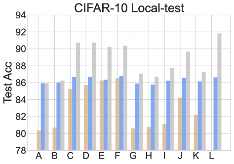
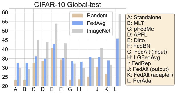
Figure 4: Effect of different initializations (Random, FedAvg model, and ImageNet pretrained model) on CIFAR-10.

Effect of $\lambda$.

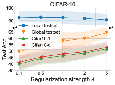
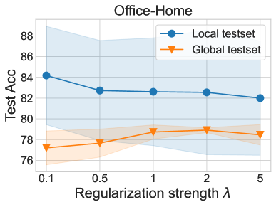
Figure 5: Effect of $\lambda$ on PerAda on CIFAR-10 and Office-Home.

Results on CIFAR-10 and Office-Home in Figure 5 shows that moderately increasing regularization strength $\lambda$ can improve generalization, but it also degrades the personalized performance, which matches the observation for $\ell_{2}$ regularization-based pFL methods in (Pillutla et al., 2022).

References

- Abadi et al. (2016) Abadi, M., Chu, A., Goodfellow, I., McMahan, H. B., Mironov, I., Talwar, K., and Zhang, L. Deep learning with differential privacy. In Proceedings of the 2016 ACM SIGSAC conference on computer and communications security, pp. 308–318, 2016.
- Acar et al. (2020) Acar, D. A. E., Zhao, Y., Matas, R., Mattina, M., Whatmough, P., and Saligrama, V. Federated learning based on dynamic regularization. In International Conference on Learning Representations, 2020.
- Arivazhagan et al. (2019) Arivazhagan, M. G., Aggarwal, V., Singh, A. K., and Choudhary, S. Federated learning with personalization layers. arXiv preprint arXiv:1912.00818, 2019.
- Ben-David et al. (2010) Ben-David, S., Blitzer, J., Crammer, K., Kulesza, A., Pereira, F., and Vaughan, J. W. A theory of learning from different domains. Machine learning, 79(1):151–175, 2010.
- Bistritz et al. (2020) Bistritz, I., Mann, A., and Bambos, N. Distributed distillation for on-device learning. Advances in Neural Information Processing Systems, 33:22593–22604, 2020.
- Bommasani et al. (2021) Bommasani, R., Hudson, D. A., Adeli, E., Altman, R., Arora, S., von Arx, S., Bernstein, M. S., Bohg, J., Bosselut, A., Brunskill, E., et al. On the opportunities and risks of foundation models. arXiv preprint arXiv:2108.07258, 2021.
- Chen & Chao (2020) Chen, H.-Y. and Chao, W.-L. Fedbe: Making bayesian model ensemble applicable to federated learning. In International Conference on Learning Representations, 2020.
- Chen & Chao (2022) Chen, H.-Y. and Chao, W.-L. On bridging generic and personalized federated learning for image classification. In International Conference on Learning Representations, 2022.
- Collins et al. (2021) Collins, L., Hassani, H., Mokhtari, A., and Shakkottai, S. Exploiting shared representations for personalized federated learning. In International Conference on Machine Learning, pp. 2089–2099. PMLR, 2021.
- Deng et al. (2020) Deng, Y., Kamani, M. M., and Mahdavi, M. Adaptive personalized federated learning. arXiv preprint arXiv:2003.13461, 2020.
- Dwork et al. (2014) Dwork, C., Roth, A., et al. The algorithmic foundations of differential privacy. Foundations and Trends® in Theoretical Computer Science, 9(3–4):211–407, 2014.
- Fallah et al. (2020) Fallah, A., Mokhtari, A., and Ozdaglar, A. Personalized federated learning: A meta-learning approach. NeurIPS, 2020.
- Foster & Rakhlin (2019) Foster, D. J. and Rakhlin, A. vector contraction for rademacher complexity. arXiv preprint arXiv:1911.06468, 6, 2019.
- Ghosh et al. (2020) Ghosh, A., Chung, J., Yin, D., and Ramchandran, K. An efficient framework for clustered federated learning. Advances in Neural Information Processing Systems, 33:19586–19597, 2020.
- Hanzely & Richtárik (2020) Hanzely, F. and Richtárik, P. Federated learning of a mixture of global and local models. arXiv preprint arXiv:2002.05516, 2020.
- Hanzely et al. (2020) Hanzely, F., Hanzely, S., Horváth, S., and Richtárik, P. Lower bounds and optimal algorithms for personalized federated learning. Advances in Neural Information Processing Systems, 33:2304–2315, 2020.
- He et al. (2016) He, K., Zhang, X., Ren, S., and Sun, J. Deep residual learning for image recognition. In Proceedings of the IEEE conference on computer vision and pattern recognition, pp. 770–778, 2016.
- Hendrycks & Dietterich (2019) Hendrycks, D. and Dietterich, T. Benchmarking neural network robustness to common corruptions and perturbations. Proceedings of the International Conference on Learning Representations, 2019.
- Hinton et al. (2015) Hinton, G., Vinyals, O., Dean, J., et al. Distilling the knowledge in a neural network. arXiv preprint arXiv:1503.02531, 2(7), 2015.
- Hsu et al. (2021) Hsu, D., Ji, Z., Telgarsky, M., and Wang, L. Generalization bounds via distillation. In International Conference on Learning Representations, 2021. URL https://openreview.net/forum?id=EGdFhBzmAwB.
- Hsu et al. (2019) Hsu, T.-M. H., Qi, H., and Brown, M. Measuring the effects of non-identical data distribution for federated visual classification. arXiv preprint arXiv:1909.06335, 2019.
- Irvin et al. (2019) Irvin, J., Rajpurkar, P., Ko, M., Yu, Y., Ciurea-Ilcus, S., Chute, C., Marklund, H., Haghgoo, B., Ball, R., Shpanskaya, K., et al. Chexpert: A large chest radiograph dataset with uncertainty labels and expert comparison. In Proceedings of the AAAI conference on artificial intelligence, volume 33, pp. 590–597, 2019.
- Jiang & Lin (2022) Jiang, L. and Lin, T. Test-time robust personalization for federated learning. arXiv preprint arXiv:2205.10920, 2022.
- Kairouz et al. (2021) Kairouz, P., McMahan, H. B., Avent, B., Bellet, A., Bennis, M., Bhagoji, A. N., Bonawitz, K., Charles, Z., Cormode, G., Cummings, R., et al. Advances and open problems in federated learning. Foundations and Trends® in Machine Learning, 14(1–2):1–210, 2021.
- Karimireddy et al. (2020) Karimireddy, S. P., Kale, S., Mohri, M., Reddi, S., Stich, S., and Suresh, A. T. Scaffold: Stochastic controlled averaging for federated learning. In International Conference on Machine Learning, pp. 5132–5143. PMLR, 2020.
- Krizhevsky et al. (2009) Krizhevsky, A., Hinton, G., et al. Learning multiple layers of features from tiny images. 2009.
- Lee et al. (2021) Lee, G., Shin, Y., Jeong, M., and Yun, S.-Y. Preservation of the global knowledge by not-true self knowledge distillation in federated learning. arXiv preprint arXiv:2106.03097, 2021.
- Li & Wang (2019) Li, D. and Wang, J. Fedmd: Heterogenous federated learning via model distillation. arXiv preprint arXiv:1910.03581, 2019.
- Li et al. (2020a) Li, T., Sahu, A. K., Zaheer, M., Sanjabi, M., Talwalkar, A., and Smith, V. Federated optimization in heterogeneous networks. Proceedings of Machine Learning and Systems, 2:429–450, 2020a.
- Li et al. (2021a) Li, T., Hu, S., Beirami, A., and Smith, V. Ditto: Fair and robust federated learning through personalization. In International Conference on Machine Learning, pp. 6357–6368. PMLR, 2021a.
- Li et al. (2020b) Li, X., Huang, K., Yang, W., Wang, S., and Zhang, Z. On the convergence of fedavg on non-iid data. In International Conference on Learning Representations, 2020b. URL https://openreview.net/forum?id=HJxNAnVtDS.
- Li et al. (2021b) Li, X., Jiang, M., Zhang, X., Kamp, M., and Dou, Q. Fedbn: Federated learning on non-iid features via local batch normalization. arXiv preprint arXiv:2102.07623, 2021b.
- Liang et al. (2020) Liang, P. P., Liu, T., Ziyin, L., Allen, N. B., Auerbach, R. P., Brent, D., Salakhutdinov, R., and Morency, L.-P. Think locally, act globally: Federated learning with local and global representations. arXiv preprint arXiv:2001.01523, 2020.
- Lin et al. (2020) Lin, T., Kong, L., Stich, S. U., and Jaggi, M. Ensemble distillation for robust model fusion in federated learning. Advances in Neural Information Processing Systems, 33:2351–2363, 2020.
- Liu et al. (2022) Liu, Z., Hu, S., Wu, Z. S., and Smith, V. On privacy and personalization in cross-silo federated learning. Advances in Neural Information Processing Systems, 2022.
- Mansour et al. (2020) Mansour, Y., Mohri, M., Ro, J., and Suresh, A. T. Three approaches for personalization with applications to federated learning. arXiv preprint arXiv:2002.10619, 2020.
- Marfoq et al. (2022) Marfoq, O., Neglia, G., Vidal, R., and Kameni, L. Personalized federated learning through local memorization. In International Conference on Machine Learning, pp. 15070–15092. PMLR, 2022.
- McMahan et al. (2017) McMahan, B., Moore, E., Ramage, D., Hampson, S., and y Arcas, B. A. Communication-Efficient Learning of Deep Networks from Decentralized Data. In Proceedings of the 20th International Conference on Artificial Intelligence and Statistics, volume 54 of Proceedings of Machine Learning Research, pp. 1273–1282. PMLR, 20–22 Apr 2017.
- Ozkara et al. (2021) Ozkara, K., Singh, N., Data, D., and Diggavi, S. Quped: Quantized personalization via distillation with applications to federated learning. Advances in Neural Information Processing Systems, 34, 2021.
- Paszke et al. (2019) Paszke, A., Gross, S., Massa, F., Lerer, A., Bradbury, J., Chanan, G., Killeen, T., Lin, Z., Gimelshein, N., Antiga, L., et al. Pytorch: An imperative style, high-performance deep learning library. Advances in neural information processing systems, 32, 2019.
- Pillutla et al. (2022) Pillutla, K., Malik, K., Mohamed, A., Rabbat, M., Sanjabi, M., and Xiao, L. Federated learning with partial model personalization. ICML, 2022.
- Rebuffi et al. (2017) Rebuffi, S.-A., Bilen, H., and Vedaldi, A. Learning multiple visual domains with residual adapters. Advances in neural information processing systems, 30, 2017.
- Recht et al. (2018) Recht, B., Roelofs, R., Schmidt, L., and Shankar, V. Do cifar-10 classifiers generalize to cifar-10? arXiv preprint arXiv:1806.00451, 2018.
- Reddi et al. (2016) Reddi, S. J., Hefny, A., Sra, S., Póczos, B., and Smola, A. Stochastic variance reduction for nonconvex optimization. In International conference on machine learning, pp. 314–323. PMLR, 2016.
- Reddi et al. (2021) Reddi, S. J., Charles, Z., Zaheer, M., Garrett, Z., Rush, K., Konečný, J., Kumar, S., and McMahan, H. B. Adaptive federated optimization. In International Conference on Learning Representations, 2021. URL https://openreview.net/forum?id=LkFG3lB13U5.
- Russakovsky et al. (2015) Russakovsky, O., Deng, J., Su, H., Krause, J., Satheesh, S., Ma, S., Huang, Z., Karpathy, A., Khosla, A., Bernstein, M., et al. Imagenet large scale visual recognition challenge. International journal of computer vision, 115(3):211–252, 2015.
- Sattler et al. (2020) Sattler, F., Müller, K.-R., and Samek, W. Clustered federated learning: Model-agnostic distributed multitask optimization under privacy constraints. IEEE transactions on neural networks and learning systems, 32(8):3710–3722, 2020.
- Scott (2014) Scott, C. Rademacher complexity. 2014. URL https://web.eecs.umich.edu/~cscott/past_courses/eecs598w14/notes/10_rademacher.pdf.
- Smith et al. (2017) Smith, V., Chiang, C.-K., Sanjabi, M., and Talwalkar, A. S. Federated multi-task learning. Advances in neural information processing systems, 30, 2017.
- Sun et al. (2021) Sun, B., Huo, H., Yang, Y., and Bai, B. Partialfed: Cross-domain personalized federated learning via partial initialization. Advances in Neural Information Processing Systems, 34, 2021.
- T Dinh et al. (2020) T Dinh, C., Tran, N., and Nguyen, J. Personalized federated learning with moreau envelopes. Advances in Neural Information Processing Systems, 33:21394–21405, 2020.
- Torralba et al. (2008) Torralba, A., Fergus, R., and Freeman, W. T. 80 million tiny images: A large data set for nonparametric object and scene recognition. IEEE transactions on pattern analysis and machine intelligence, 30(11):1958–1970, 2008.
- Venkateswara et al. (2017) Venkateswara, H., Eusebio, J., Chakraborty, S., and Panchanathan, S. Deep hashing network for unsupervised domain adaptation. In Proceedings of the IEEE conference on computer vision and pattern recognition, pp. 5018–5027, 2017.
- Wang & Joshi (2019) Wang, J. and Joshi, G. Cooperative sgd: A unified framework for the design and analysis of communication-efficient sgd algorithms. In ICML Workshop on Coding Theory for Machine Learning, 2019.
- Wolf et al. (2020) Wolf, T., Debut, L., Sanh, V., Chaumond, J., Delangue, C., Moi, A., Cistac, P., Rault, T., Louf, R., Funtowicz, M., Davison, J., Shleifer, S., von Platen, P., Ma, C., Jernite, Y., Plu, J., Xu, C., Scao, T. L., Gugger, S., Drame, M., Lhoest, Q., and Rush, A. M. Transformers: State-of-the-art natural language processing. In Proceedings of the 2020 Conference on Empirical Methods in Natural Language Processing: System Demonstrations, pp. 38–45, Online, October 2020. Association for Computational Linguistics. URL https://www.aclweb.org/anthology/2020.emnlp-demos.6.
- Wu et al. (2020) Wu, B., Xu, C., Dai, X., Wan, A., Zhang, P., Yan, Z., Tomizuka, M., Gonzalez, J., Keutzer, K., and Vajda, P. Visual transformers: Token-based image representation and processing for computer vision, 2020.
- Zhang et al. (2021) Zhang, J., Guo, S., Ma, X., Wang, H., Xu, W., and Wu, F. Parameterized knowledge transfer for personalized federated learning. Advances in Neural Information Processing Systems, 34:10092–10104, 2021.
- Zhang et al. (2022) Zhang, L., Shen, L., Ding, L., Tao, D., and Duan, L.-Y. Fine-tuning global model via data-free knowledge distillation for non-iid federated learning. In Proceedings of the IEEE/CVF Conference on Computer Vision and Pattern Recognition, pp. 10174–10183, 2022.
- Zhu et al. (2021) Zhu, Z., Hong, J., and Zhou, J. Data-free knowledge distillation for heterogeneous federated learning. In International Conference on Machine Learning, pp. 12878–12889. PMLR, 2021.