Multiple Instance Learning with Trainable Decision Tree Ensembles

Abstract

A new random forest based model for solving the Multiple Instance Learning (MIL) problem under small tabular data, called Soft Tree Ensemble MIL (STE-MIL), is proposed. A new type of soft decision trees is considered, which is similar to the well-known soft oblique trees, but with a smaller number of trainable parameters. In order to train the trees, it is proposed to convert them into neural networks of a specific form, which approximate the tree functions. It is also proposed to aggregate the instance and bag embeddings (output vectors) by using the attention mechanism. The whole STE-MIL model, including soft decision trees, neural networks, the attention mechanism and a classifier, is trained in an end-to-end manner. Numerical experiments with tabular datasets illustrate STE-MIL. The corresponding code implementing the model is publicly available.

Keywords: multiple instance learning, decision tree, oblique tree, random forest, attention mechanism, neural network

1 Introduction

Many machine learning real-life applications deal with labeled objects called bags, which consist of several instances such that individual labels of the instances contained in the bags are not provided, for example, in histopathology, the histology images can be viewed as bags and its patches (cells) as instances of the bag [1, 2, 3]. One can find many similar application examples, for example, the drug activity prediction [4], detecting the lung cancer [5], the protein function annotation [6]. A useful frameworks for modeling the applications is the Multiple Instance Learning (MIL) which can be regarded as a type of weakly supervised learning [7, 8, 9, 10, 11, 12, 13]. A goal of MIL is to classify new bags based on training data consisting of a set of labeled bag and to assign labels to unlabeled instances in the bags. In order to achieve the goal, assumptions or rules are introduced to establish relationship between labels of instances and the corresponding bag. Most MIL models assume that all negative bags contain only negative instances, and that positive bags contain at least one positive instance. However, there are also other rules of the bag label definitions [14].

There are many MIL models which try to solve the problem under different conditions and for different types of datasets [15, 16, 17, 18, 19, 20]. Most above models use such methods as SVM, K nearest neighbors, convolutional neural networks, decision trees. An interesting and efficient class of the MIL models applies the attention mechanism [21, 22, 23, 24, 25, 26, 27].

However, there are some disadvantages of the above approaches to MIL. First, simple models based on such methods as SVM, decision trees, etc. do not use neural network and cannot have several advantages of the network models, for example, the end-to-end training and the attention mechanism. On the other hand, the MIL models based on neural networks cannot be accurately trained on small tabular datasets.

Therefore, the MIL model which simultaneously has properties of the random forest (RF) and neural network can provide better results in comparison with the available model. RF directly fit a MIL model because it is robust to noise in target variables. At the same time, its structure is suboptimal, therefore, it does not minimize the MIL loss in some cases. One of the ways to construct decision trees, which can be retrained, is a concept of soft oblique trees [28] whose trainable parameters can be updated and optimize by using the gradient algorithms. Oblique trees and RFs composed from oblique trees use linear and non-linear classifiers at each split in the decision trees and allow us to combine more than one feature at a time. However, when we deal with small tabular data, soft oblique trees may overfit due to a large number of parameters.

Therefore, we propose to represent soft oblique trees in the form of classic decision trees and to convert the decision trees, which comprise RF, into the trainable neural networks of a special way. The corresponding neural networks implement approximately the same functions as the decision trees, but they can be effectively trained jointly with the attention mechanism and can simultaneously take into account data from all bags, i.e., they successfully solve the MIL problem.

In sum, we propose an attention MIL model called Soft Tree Ensemble (STE-MIL). On the one hand, STE-MIL is based on decision trees and successfully deals with small tabular data. On the other hand, after converting trees into neural networks and applying the attention mechanism to aggregate embedding of instances and bags, STE-MIL is trained by using gradient descent algorithms in an end-to-end manner.

Our contributions can be summarized as follows:

1. A new RF-based MIL model, which outperforms many MIL models when dealing with small tabular data, is proposed.

2. A new type of soft decision trees similar to the soft oblique trees is proposed. In contrast to the soft oblique trees, the proposed trees have a smaller number of trainable parameters. Nevertheless, it can be trained in the same way as the soft oblique trees. Outputs of each soft decision tree are viewed as a set of vectors (embedding) which are formed from the class probability distributions in a specific way.

3. An original algorithm for converting the decision trees into neural networks of a specific form for efficient training parameters of the trees is proposed.

4. The attention is proposed to aggregate the instance and bag embeddings with aim to minimize the corresponding loss function.

5. The whole MIL model, including soft decision trees, neural networks, the attention mechanism and a classifier, is trained in an end-to-end manner.

6. Numerical experiments with well-known datasets Musk1, Musk2 [4], Fox, Tiger, Elephant [15] illustrate STE-MIL. The above datasets have numerical features that are used to perform tabular data. The corresponding code implementing the model is publicly available at https://github.com/andruekonst/ste_mil.

The paper is organized as follows. Related work can be found in Section 2. A brief introduction to MIL and the oblique binary soft trees is given in Section 3. A specific representation of the decision tree function, which allows us to convert the decision tree to a neural network, is proposed in Section 4. A soft tree ensemble for solving the MIL problem is considered in Section 5. An algorithm for converting the decision trees into neural networks are studied in the same section. The attention mechanism applied to the proposed MIL models is studied in Section 6. Numerical experiments are provided in Section 7. Concluding remarks can be found in Section 8.

2 Related work

MIL. The MIL can be regarded as an important tool for dealing with different types of data. In particular, tabular data of a specific structure can be also classified by means of the MIL models. Therefore, if to consider tabular data, then several available MIL models are based on the applying such models as SVM, decision trees, AdaBoost, RFs [15, 16, 29, 19, 20].

However, most MIL models are based on applying neural networks or convolutional neural network, especially, when image datasets are classified [30, 31, 17, 32, 18, 19, 33].

In spite of various available MIL models, there are no models which could combine the tabular data oriented models like RFs and neural networks, including the attention mechanism, in order to use the gradient-based algorithm for updating training parameters of RFs as well as neural networks and to improve accuracy of the MIL predictions.

MIL and attention. Several MIL models using the attention mechanism have been proposed in order to enhance the classification accuracy. Examples of the models are SA-AbMILP (Self-Attention Attention-based MIL Pooling) [34], ProtoMIL (Multiple Instance Learning with Prototypical Parts) [26], MHAttnSurv (Multi-Head Attention for Survival Prediction) [24], AbDMIL [23], MILL (Multiple Instance Learning–based Landslide classification) [35], DSMIL (Dual-Stream Multiple Instance Learning) [36]. The attention-based MIL models can be also found in [22, 21, 37, 38, 27]. The main peculiarity of the above mentioned models is that they use neural networks and mainly deal with the image data, but not with small tabular data.

Oblique trees and neural networks. Many studies have demonstrated that trees with oblique splits produce smaller trees with better accuracy compared with axis parallel trees in many cases [39, 40]. One of the important advantages of oblique trees is that they can be trained by using optimization algorithms, for example, the gradient descent algorithm. On the other hand, some obstacles of training the oblique trees can be met. In particular, the training procedure is computationally expensive. Moreover, the corresponding model may be overfitted. Several approaches have been proposed to partially solve the above problems. Wickramarachchi et al. [40] present a new decision tree algorithm, called HHCART. In order to simplify oblique trees, Carreira-Perpinan and Tavallali [41] propose an algorithm called sparse oblique trees, which produces a new tree from the initial oblique tree having the same or smaller structure, but new parameter values leading to a lower or unchanged misclassification error. One-Stage Tree as a soft tree to build and prune the decision tree jointly through a bi-level optimization problem is presented in [42]. Menze at al. [43] focus on trees with task optimal recursive partitioning. Katuwal et al. [44] propose a random forest of heterogeneous oblique decision trees that employ several linear classifiers at each non-leaf node on some top ranked partitions. An application of evolutionary algorithms to the problem of oblique decision tree induction is considered in [45]. An algorithm improving learning of trees through end-to-end training with backpropagation was presented in [46].

An interesting direction of using the oblique trees is to represent neural networks as the trees or trees in the form of neural networks. Lee at al. [47] show how neural models can be used to realize piece-wise constant functions such as decision trees. Hazimeh et al. [48] propose to combine advantages of neural networks and tree ensembles by designing a hybrid model by considering the so-called tree ensemble layer for neural networks, which is an additive model of differentiable decision trees. The layer can be inserted anywhere in a neural network, and is trained along with the rest of the network using gradient-based algorithms. Frosst and Hinton [49] take the knowledge acquired by a neural net and express the same knowledge in a model that relies on hierarchical decisions instead, explaining a particular decision would be much easier. A way of using a trained neural net to create a type of soft decision tree that generalizes better than one learned directly from the training data is also provided in [49]. Karthikeyan et al. [50] proposed a unified method that enables accurate end-to-end gradient based tree training and can be deployed in a variety of settings. Madaan et al. [51] presented dense gradient trees and an transformer based on the trees, which is called Treeformer.

In contrast to the above work, we consider how to apply decision trees to the MIL problem by converting the trees into neural networks of a special form and by training them jointly with the attention mechanism in the end-to-end manner.

3 Preliminary

3.1 Multiple Instance Learning

First, we formulate the MIL classification problem. It differs from the standard classification by the data structure. Namely, in the MIL problem, bags have class labels, but instances, which compose each bags, are usually unlabeled. This problem can be regarded as a kind of the weakly supervised learning problem. Due to the availability of labels only for bags, the following tasks can be stated in the framework of the MIL. The first task concerns with annotation of instances from a bag. The second task aims to classify new bags by having a training set of bags. The above tasks can be solved by introducing special rules which establish the relationship between the instance and bag class labels.

Let us formally state the MIL problem taking into account the rules connecting different levels of the MIL data consideration. Suppose that each bag is defined by a set of $m$ feature vectors $\mathbf{X}=\{\mathbf{x}_{1},...,\mathbf{x}_{n}\}$, where $\mathbf{x}_{i}\in\mathbb{R}^{m}$ is a feature vector representing the $i$-th instance. Each instance $\mathbf{x}_{i}$ has a label $y_{i}\in\{0,1\}$ taking two values: $0$ (negative class) and $1$ (positive class). We do not know labels $y_{i}$ during training as it follows from the MIL problem statement. According to the first task, we have to construct a function $g$ which maps each vector $\mathbf{x}_{i}$ into label $y_{i}$.

There are various rules establishing the relationship between labels of bags and instances. One of the most common rules can be rewritten as follows [9]:

$$f(\mathbf{X})=\left\{\begin{array}[c]{cc}1,&\exists\mathbf{x}\in\mathbf{X}:g(\mathbf{x})=1,\\ 0,&\text{otherwise,}\end{array}\right.$$ (1)

where $f(\mathbf{X})$ is a bag classifier.

It follows from (1) that at least one positive instance makes the bag positive, and negative bags contain only negative instances. Function $f(\mathbf{X})$ can be defined in another way taking into account a threshold $\theta$ as

$$f(\mathbf{X})=\left\{\begin{array}[c]{cc}1,&\theta\leq\sum_{\mathbf{x}\in\mathbf{X}}g(\mathbf{x}),\\ 0,&\text{otherwise.}\end{array}\right.$$ (2)

We will use the rule defined in (1).

The dataset can be represented as

$$\mathcal{D}=\left\{\left(\{\mathbf{x}_{k}^{(i)}\}_{k=1}^{n_{i}},y_{i}\right)\right\}_{i=1}^{N},$$ (3)

where $\mathbf{x}_{k}^{(i)}$ is the $k$-th instance vector belonging to the $i$-th bag; $n_{i}$ is the number of instances in the $i$-th bag; $N$ is the number of labelled bags in the training set.

Rule (1) defining the function $f$ can be represented through the MIL maximal pooling operator as follows:

$$f(\{\mathbf{x}_{k}^{(i)}\}_{k=1}^{n_{i}})=\max\left\{g(\mathbf{x}_{k}^{(i)})\right\}_{k=1}^{n_{i}}.$$ (4)

Hence, the binary classification loss, which is minimized, can be written as

$$\mathcal{L}=\frac{1}{N}\sum_{i=1}^{N}l(y_{i},f(\{\mathbf{x}_{k}^{(i)}\}_{k=1}^{n_{i}}))=\frac{1}{N}\sum_{i=1}^{N}l(y_{i},\max\{g(\mathbf{x}_{k}^{(i)})\}_{k=1}^{n_{i}}).$$ (5)

3.2 Oblique binary soft trees

One of the important procedures to build oblique decision trees is optimization of their parameters. There are various decision rules for building trees. The so-called hard decision rules have been successfully implemented in [50] and [51]. The rules are applied to the oblique decision trees which may be improper when we deal with small tabular datasets, because large degrees of freedom in this case would lead to overfitting.

According to [50], an oblique binary tree of height $h$ represents a piece-wise constant function $f(\mathbf{x};\mathbf{W},\mathbf{b}):\mathbb{R}^{m}\rightarrow\mathbb{R}^{K}$ parameterized by weights $\mathbf{w}_{I(d,l)}\in\mathbb{R}^{m}$, $b_{I(d,l)}\in\mathbb{R}$ at a node on the path from the tree root to its leaf $l$ at depth $d$. Here $I(d,l)$ is the index of a node on the path from the tree root to its leaf $l$ with depth $d$. Function $f$ computes decision functions of the form $\mathbf{w}_{j}^{\mathrm{T}}\mathbf{x}-b_{j}>0$, that define whether $\mathbf{x}$ must traverse the left or right child next. Here $\mathbf{W}$ is the parameter matrix consisting of all parameter vectors $\mathbf{w}_{j}$; $\mathbf{b}$ is the parameter vector consisting of parameters $b_{j}$. The tree output is represented as $2^{h}$ vectors $\theta_{1},...,\theta_{2^{h}}$ such that vector $\theta_{j}$ $\in\Delta^{K}$ at the $j$-th leaf is associated with probabilities of $K$ classes, where $\mathbb{\Delta}^{K}$ is the unit simplex of dimension $K$. One of the ways for learning parameters $\mathbf{w}_{ij}$ and $b_{ij}$ for all nodes is to minimize the expected loss $l$ of the form:

$$\min_{\mathbf{W},\mathbf{b}}\sum_{i=1}^{n}l(y_{i},f(\mathbf{x};\mathbf{W},\mathbf{b})).$$ (6)

Karthikeyan et al. [50] propose the following function $f(\mathbf{x};\mathbf{W},\mathbf{b})$:

$$f_{\theta}(\mathbf{x};\mathbf{W},\mathbf{b})=\sum_{l=1}^{2^{h}}q_{l}(\mathbf{x},\mathbf{W},\mathbf{b})\theta_{l},$$ (7)

where the tree path indicators $q_{l}(\mathbf{x},\mathbf{W},\mathbf{b})$ are represented as the following indicator function:

$$q_{l}(\mathbf{x},\mathbf{W},\mathbf{b})=\mathbb{I}\left[\bigwedge\limits_{d=1}^{h}([\mathbf{w}_{I(d,l)}^{\mathrm{T}}\mathbf{x}\leq b_{I(d,l)}]\oplus s(d,l))\right],$$ (8)

Here $\mathbb{I}(\cdot)$ is the indicator function taking the value $1$ of its argument is non-negative, otherwise it is $0$; $\oplus$ is the operator XOR; $s(d,l)$ determines whether the predicate of a node on the path to the leaf $l$ at the depth $d$ should be evaluated to be true or false, i.e., $s(d,l)=1$ if the $l$-th leaf belongs to the left subtree of node $I(d,l)$, otherwise $s(d,l)=0$. It is well known that the conjunction in (8) can be replaced with the product as follows:

$$q_{l}(\mathbf{x},\mathbf{W},\mathbf{b})=\prod_{d=1}^{h}\mathbb{I}\left[[\mathbf{w}_{I(d,l)}^{\mathrm{T}}\mathbf{x}\leq b_{I(d,l)}]\oplus s(d,l)\right].$$ (9)

However, this representation significantly complicates the optimization of the model by using the gradient descent algorithm due to the vanishing gradient problem. Another representation of $q_{l}(\mathbf{x},\mathbf{W},\mathbf{b})$ is proposed in [50]. It is of the form:

$$q_{l}(\mathbf{x},\mathbf{W},\mathbf{b})=\sigma\left(\sum_{d=1}^{h}\sigma\left[[\mathbf{w}_{I(d,l)}^{\mathrm{T}}\mathbf{x}\leq b_{I(d,l)}]\oplus s(d,l)\right]-h\right),$$ (10)

where the indicator functions are replaced with the so-called $\sigma$-hard indicator approximations [50] which apply quantized functions in the forward pass, but uses a smooth activation function in the backward pass to propagate. This specific representation of the sigmoid function is called the straight-through operator and proposed in [52].

This representation allows us to effectively apply the gradient descent algorithm to compute optimal parameters of the tree in accordance with the loss function (6).

The soft tree concept proposed in [50] and [51] is an interesting approach to deal with small tabular data. However, our experiments with soft trees have demonstrated that it is difficult to train the oblique soft trees for some datasets. Therefore, we propose to modify the standard decision trees to implement them in the form of neural networks.

4 A softmax representation of the decision tree function

In order to overcome difficulties of training the oblique decision tree, we propose another its representation which allows us to effectively update it. Let us consider a complete binary decision tree $f_{\theta}$ of depth $h$:

• the tree has $(2^{h}-1)$ non-leaf nodes parametrized by $(\mathbf{w}_{j},b_{j})$, where

  • $\mathbf{w}_{j}$ is an one-hot vector having $1$ at the position corresponding to the node feature;

  • $b_{j}$ is a threshold;

• the tree has also $2^{h}$ leaves with values $\mathbf{v}_{l}$, where $\mathbf{v}_{l}$ is an output vector corresponding to the $j$-th leaf.

In contrast to representation (10) of function $q_{l}$, we propose to avoid the direct comparison with the height of a tree, because this representation requires the indicator approximation to return integer values, otherwise the $q_{l}$ will always be evaluated to be zero. If we would use (10) instead of the softmax function, then (7) will provide the sum of the leaf vectors in place of selecting one of them. We use the softmax function to guarantee a convex combination of the leaf vectors. We replace the outer indicator with the softmax function having the trainable temperature parameter $\tau$:

$$q_{l}(\mathbf{x},\mathbf{W},\mathbf{b},\tau,\omega)=\mathrm{softmax}_{\tau}\left(\sum_{d=1}^{h}\sigma_{\omega}\left[[-\mathbf{w}_{I(d,l)}^{\mathrm{T}}\mathbf{x}+b_{I(d,k)}]\cdot\hat{s}(d,k)\right]\right)_{k=1}^{2^{h}},$$ (11)

where $\hat{s}(d,k)\in\{-1,1\}$ is the node sign; $\sigma$ is the sigmoid with the trainable temperature or scaling parameter $\omega$.

The proposed representation could be interpreted as selecting the most appropriate path among all candidate paths. Neural trees defined by using the above representation can be optimized by means of the stochastic gradient descent algorithm with the fixed node weights $\mathbf{w}_{j}$, i.e., by updating only thresholds, the softmax temperature parameters $\tau$, the sigmoid temperature parameters $\omega$ and leaf values.

5 Soft Tree Ensemble for MIL

One of the possible ways for solving the MIL classification problem, i.e., for constructing the instance model $\tilde{g}$, is to assign a bag label to all instances belonging to the bag. In this case, we get a new instance-level dataset with the repeated instance labels, which is of the form:

$$\tilde{\mathcal{D}}=\{\left(\mathbf{x}_{k}^{(i)},y_{i}\right)~{}|~{}k=1,...,n_{i}\}_{i=1}^{N}.$$ (12)

According to [53], RF can be regarded as a desirable MIL classifier even if it is trained on artificially made instance-level datasets like (12) because RF is inherently robust to noise in the target variable. After training on dataset (12), parameters of the built RF can be seen as a suboptimal solution to the optimization problem defined by the bag-level loss (5). In the extremely worst case, RF is totally overfitted, i.e. it just remembers the bag label for each instance.

There are approaches that try to repeatedly infer the instance labels by using a trained RF, and then retrain the RF on obtained instance labels. One of the approaches is implemented in the so-called MIForests [53]. The main problem of the results is that the methods rebuild decision trees instead of updating them, partially losing useful tree structures obtained at different steps.

5.1 Soft Tree Ensemble

A key idea behind STE-MIL can be represented in the form of the following schematic algorithm:

1. Let us assign incorrect labels to instances of a bag, for example, the same as a label of the corresponding bag. The instance labels may be incorrect because we do not know true labels and their determination is our task. However, these labels are needed to build an initial RF. This is a kind of the initialization procedure for the whole model which is trained in the end-to-end manner.

2. The next step is to convert the initial RF to a neural network having a specific architecture. To implement this step, non-leaf nodes of each tree in RF are parametrized by trainable parameters $\mathbf{b}$, $\tau$, $\omega$, and non-trainable parameters $\mathbf{W}$.

3. Parameters of the tree nodes $\mathbf{b}$, $\tau$, $\omega$ are updated by using the stochastic gradient descend algorithm to minimize the bag loss defined in (5). To implement the updating algorithm, we propose to approximate the tree path indicators $q_{l}(\mathbf{x},\mathbf{W},\mathbf{b},\tau,\omega)$ by using a specific softmax representation (11). This is a key step of the algorithm which allows us to update trees by updating neural networks and incorporate the trees or RF in the whole scheme of modules, including the attention mechanism and a classifier.

Suppose that RF consisting of $T$ decision trees has been trained on repeated instance labels (12). We convert its trees to a set of $T$ neural networks which implement functions $f^{(1)}(\mathbf{x}),\dots,f^{(T)}(\mathbf{x})$ such that the $i$-th tree corresponds to the $i$-th network implementing function $f^{(i)}(\mathbf{x})$. After converting trees to neural networks, we can update their parameters to minimize the bag-level loss (5). The ensemble prediction for a new instance $\mathbf{x}$ is defined as follows:

$$f(\mathbf{x})=\frac{1}{T}\sum_{i=1}^{T}f^{(i)}(\mathbf{x}).$$ (13)

The bag prediction can be obtained by applying any aggregation function $G$:

$$f(\{\mathbf{x}_{k}^{(i)}\}_{i=1}^{N})=G(f(\mathbf{x}_{1}^{(i)}),\dots,f(\mathbf{x}_{n_{i}}^{(i)})).$$ (14)

The next questions is how to convert the decision trees into neural networks.

5.2 Trees to Neural Networks

Suppose that RF is trained on artificial dataset (12). Then it can be converted to a neural network with a specific structure. A tree with $M$ internal decision nodes and $L$ leaves is represented as a neural network with three layers:

1. The first layer aims to approximate the node predicates. It is a fully connected layer with $m$ inputs (dimensionality of $\mathbf{x}$) and $M$ outputs, i.e., there holds:

   $$f^{(1)}(\mathbf{x})=\sigma\left(\mathbf{Wx}+\mathbf{b}~{}|~{}\omega\right),$$ (15)

   where $\mathbf{W}\in\mathbb{R}^{r\times m}$ is a matrix of non-trainable parameters consisting of $r$ vectors $\mathbf{w}_{i}\in\mathbb{R}^{m}$; $r$ is the total number of the tree nodes; $\mathbf{b}\in\mathbb{R}^{r}$ is the trainable bias vector; $\omega$ is the trainable temperature parameter of the sigmoid $\sigma$.

   In sum, the first layer has only trainable parameters $\mathbf{b}$ and $\omega$. The matrix $\mathbf{W}$ consists of the one-hot vectors having $1$ at positions corresponding to the node features.

2. The second layer aims to estimate the leaf indices. It is fully connected layer with $M$ inputs and $L$ outputs having one trainable parameter $\tau$:

   $$f^{(2)}(\xi)=\text{softmax}(\mathbf{R\xi}+\mathbf{s}~{}|~{}\tau),$$ (16)

   where $\mathbf{R}\in\mathbb{R}^{L\times M}$ is a non-trainable routing matrix that encodes decision paths such that one path forms one row of $\mathbf{R}$; $\mathbf{\xi}\in\mathbb{R}^{M}$ is the input vector; $\mathbf{s}\in\mathbb{R}^{L}$ is the non-trainable bias vector; $\tau$ is the trainable temperature parameter of the softmax operation.

   Matrix $\mathbf{R}$ consists of values from the set: $\{-1,0,1\}$. If the path to $i$-th leaf does not contain $j$-th node, then $R_{i,j}=0$. Otherwise, if the path goes to the left branch, then $R_{i,j}=-1$, and $R_{i,j}=1$ if the path goes to the right branch. Vector $\mathbf{s}=(s_{1},...,s_{2^{h}})$ is needed to balance the decision paths. The sum of the sigmoid functions for the path to the $k$-th leaf in (11) can be represented as:

   $$\sum_{d=1}^{h}\sigma\left([-\mathbf{w}_{I(d,l)}^{\mathrm{T}}\mathbf{x}+b_{I(d,k)}]\cdot\hat{s}(d,k)\right)$$

   $$=\sum_{i=1}^{M}\left(R_{k,i}\sigma\left(-\mathbf{w}_{I(d,l)}^{\mathrm{T}}\mathbf{x}+b_{I(d,k)}\right)+\mathbb{I}\left[R_{k,i}=-1\right]\right)$$

   $$=\sum_{i=1}^{M}\left(R_{k,i}\sigma\left(-\mathbf{w}_{I(d,l)}^{\mathrm{T}}\mathbf{x}+b_{I(d,k)}\right)\right)+s_{k},$$ (17)

   because there holds $\sigma(-\omega)=1-\sigma(\omega)$.

3. The third layer aims to calculate the output values (embeddings). It is trainable and fully connected. Each leaf generates the class probability vector of size $C$. We take the probability $v_{1}(\mathbf{x})$ of class 1 and repeat it $E-1$ times such that the whole embedding $\mathbf{v}(\mathbf{x})=(v_{1}^{(1)}(\mathbf{x}),...,v_{1}^{(E)}(\mathbf{x}))$ has the length $E$. The final output of the network (or the third layer) is of the form

   $$f(\mathbf{x})=\mathbf{V}f^{(2)}\left(f^{(1)}(\mathbf{x})\right),$$ (18)

   where $\mathbf{V}\in\mathbb{R}^{E\times L}$ is a trainable leaf value matrix consisting of $L$ vectors $\mathbf{v}(\mathbf{x})$.

An example of the transformation of a tree to a neural network is illustrated in Fig. 1. The full decision tree with three decision nodes and four leaves is considered and depicted in Fig. 1. The first layer of the neural network computes all decisions at internal nodes of the tree. Matrix $\mathbf{R}$ is constructed such that each its row represents a path to the corresponding leaf of the tree. For example, values of the first row are $(-1,-1,0)$ because the path to the leaf $l_{1}$ passes through the nodes $d_{1}$ and $d_{2}$ to the left. Values of the third row are $(1,0,-1)$ because the path to the third leaf $l_{3}$ passes through the node $d_{1}$ to the right, and it does not pass through the node $d_{2}$ and passes through the node $d_{3}$ to the left. Elements of vector $\mathbf{s}$ are equal to number of left turns, which is equivalent to the number of values $-1$ at the corresponding row of $\mathbf{R}$.

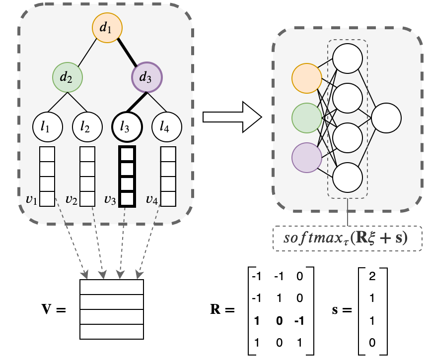
Figure 1: Forming the second layer through matrix $\mathbf{R}$

The class distribution provided by a tree is computed by counting the percentage of different classes of instances at the leaf node where the concerned instance falls into. Formally, the leaf value vectors are initially estimated for the $l$-th leaf of the $j$-tree as follows:

$$\mathbf{v}_{j}^{(l)}(\mathbf{x})=\left(\frac{\#\{(k,i)\in J(l)|y_{i}=1\}}{\#J(l)}\right)_{t=1}^{E},$$ (19)

where $J(l)$ is an index set of training points which fall into the $l$-th leaf.

We use constant matrix $\mathbf{W}$ that represents decision nodes, in order to preserve the axis parallel decision planes. It is initialized as the one-hot encoded representation of decision tree split features. Only the bias $\mathbf{b}$ of the first layer of the neural network is trainable, and is initialized with the negative values of the decision tree split thresholds.

Matrix $\mathbf{V}$ of the leaf values is initialized with repeated tree leaf values, i.e., each its column contains the same values equal to the original tree leaf value.

The algorithm for the routing matrix $\mathbf{R}$ construction is shown as Algorithm 1.

Algorithm 1 Recursive $\bf{R}$ matrix construction

procedure FILL($\bf{R}$, $a$, $b$, $k$)

     if $k>M$ then return

     end if

     $d\leftarrow\lfloor\frac{b-a}{2}\rfloor$ $\triangleright$ A half of the input row index span $[a,b]$

     for $i\leftarrow a$ to $a+d$ do

         $R_{i,k}\leftarrow-1$ $\triangleright$ Fill first $d$ rows with $-1$

         $R_{i,d+k}\leftarrow 1$ $\triangleright$ Fill second $d$ rows with $1$

     end for

     FILL($\bf{R}$, $a$, $a+d$, $2k$) $\triangleright$ Recursively fill the first $d$ rows, left subtree

     FILL($\bf{R}$, $a+d$, $b$, $2k+1$) $\triangleright$ Fill the second $d$ rows, right subtree

end procedure

$\mathbf{R}\leftarrow\mathbf{0}\in\mathbb{R}^{L\times M}$ $\triangleright$ Initialize matrix with zeros

FILL($\bf{R}$, $a=1$, $b=L$, $k=1$)

5.3 Peculiarities of the proposed soft trees

• The sigmoid and softmax temperature parameters are trained starting from value $0.1$ to avoid having to fit them as hyperparameters. Temperatures as trainable parameters are not redundant because the first layer of the neural network contains a fixed weight matrix $\mathbf{W}$, so $\mathbf{Wx}+\mathbf{b}$ cannot be equivalent to $\tau(\mathbf{Wx}+\mathbf{b})$. The same take place with the softmax operation which contains a fixed number of terms from $0$ to $1$.

• In contrast to [50], we do not use oblique trees as they may lead to overfitting on tabular data. Trees with the axis-parallel separating hyperplanes allow us to build accurate models for tabular data where linear combinations of features often do not make sense.

• Therefore, we also do not use overparametrization, which is a key element for convergence of training the decision trees with quantized decision rules (when the indicator is represented not by a sigmoid function, but by the so-called straight-through operator [52]).

• We use softmax as an approximation of argmax instead of the approximation of the sum of indicator functions. At the prediction stage, the implementation of the algorithm proposed in [50], which uses the sigmoid function, could predict the sum of the values at several leaves at the same time.

Further, we can reduce the temperature $\omega$ so that the decision rules become more stringent. Unfortunately, it is not working in practice because, by a rather large depth ($h>3$), on the same path, inconsistent rules are often learned, which give the “correct” values by low temperatures and degenerate by small $\omega$. As a result, the accuracy starts to decrease as $\omega$ decreases. If we do not decrease $\omega$, then the trees may become not axis-parallel.

6 Attention and the whole scheme of STE-MIL

After training, output of each neural network corresponding to the $k$-th tree is the embedding $\mathbf{v}_{j,k}^{(i)}$ of length $E$, where $i$ and $j$ are indices of the corresponding bag and instance in the bag, respectively. This implies that we get $T$ embeddings $\mathbf{v}_{j,1}^{(i)},...,\mathbf{v}_{j,T}^{(i)}$ for the $j$-th instance from the $i$-th bag, $j=1,...,n$, $i=1,...,N$, under assumption of the identical number of trees in all RFs. It should be noted that numbers of trees in RFs can be different. However, we consider the same numbers for simplicity.

Embeddings $\mathbf{v}_{i,1},...,\mathbf{v}_{i,T}$ are aggregated by using, for example, the averaging operation, resulting vectors $\mathbf{e}_{j}^{(i)}$, $j=1,...,n$, corresponding to the $i$-th bag. Then aggregated embeddings $\mathbf{e}_{1}^{(i)},...,\mathbf{e}_{n}^{(i)}$ are attended in order to get a final representation of the $i$-th bag in the form of vector $\mathbf{a}_{i}$, which is classified. This motivates us to replace the class probability distributions at the tree leaves with the embeddings $\mathbf{v}$ defined above. We can define several ways for constructing embeddings from the class probability distributions. However, we select a simple procedure which has demonstrated its efficiency from the accuracy and computational points of view.

Hence, the second idea behind STE-MIL is to aggregate the embeddings over all bags by using the attention mechanism and to calculate the prediction logits by linear projecting the aggregated embedding to the one-dimensional space. This idea is also motivated by the Attention-MIL approach proposed in [23] and by the Multi-attention multiple instance learning model proposed in [25], which may help to train a better bag-level classifier. A scheme of the whole STE-MIL model is shown in Fig. 2. It can be seen from Fig. 2 that each instance ($\mathbf{x}_{j}^{(i)}$) from the $i$-th bag learns the corresponding RF such that embeddings are combined to the aggregated vector $\mathbf{e}_{j}^{(i)}$. Vectors $\mathbf{e}_{j}^{(i)}$, $j=1,...,n_{i}$, can be regarded as keys in terms of the attention and are attended and produce vector $\mathbf{a}_{i}$ which is the input of the classifier. The whole system is trained on all instances from all bags.

The attention module produces a new aggregate embedding $\mathbf{a}_{k}$ corresponding to the $k$-th bag, which is computed as follows:

$$\mathbf{a}_{k}=\sum_{i=1}^{n}\beta_{i}^{(k)}\mathbf{e}_{i}^{(k)},\ k=1,...,N,$$ (20)

where

$$\beta_{i}^{(k)}=\mathrm{softmax}\left(\mathbf{q}^{\mathrm{T}}\mathbf{k}_{i}\right),$$ (21)

$$\mathbf{q=V}_{q}\mathbf{g},\ \mathbf{k}_{i}\mathbf{=V}_{k}\mathbf{e}_{i}^{(k)}.$$ (22)

Here $\mathbf{V}_{k}$ and $\mathbf{V}_{q}$ are the trainable weight matrices for $\mathbf{e}_{i}^{(k)}$ (keys) and the template vector $\mathbf{g}$ (query), respectively.

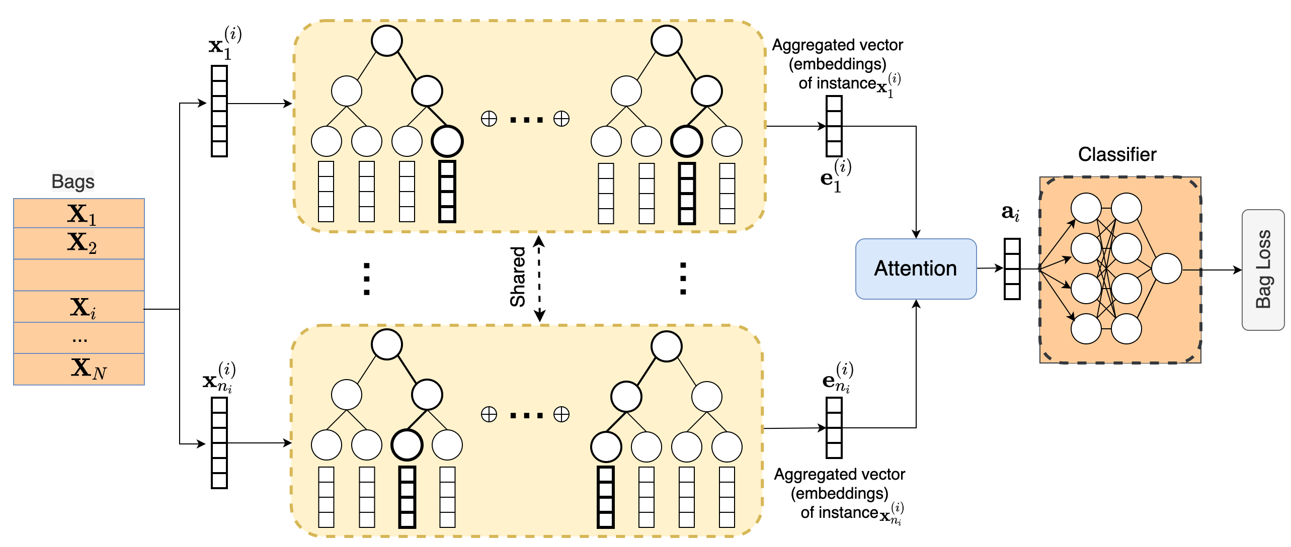
Figure 2: A scheme of the ensembled STE-MIL

7 Numerical experiments

In order to compare the proposed model with other MIL classification models, we train the corresponding models on datasets Musk1, Musk2 (drug activity) [4], Fox, Tiger, Elephant [15]. Table 1 shows the number of bags $N$, the number of instances $n$ in every bag and the number of features $m$ in instances for the corresponding datasets. The Musk1 dataset contains 92 bags consisting of 476 instances with 166 features. The average bag size is $5.17$. The Musk2 dataset contains 102 bags consisting of 6598 instances with 166 features. The average bag size is $64.69$. Each dataset (Fox, Tiger and Elephant) contains exactly 200 bags consisting of instances with 230 features. Numbers of instances in datasets Fox, Tiger and Elephant are 1302, 1220 and 1391, respectively. The average bag sizes of the datasets are $6.60$, $6.96$ and $6.10$, respectively.

The accuracy measures for these datasets are also obtained by means of the well-known MIL classification models, including mi-SVM [15], MI-SVM [15], MI-Kernel [54], EM-DD [55], mi-Graph [56], miVLAD [57], miFV [57], mi-Net [19], MI-Net [19], MI-Net with DS [19], MI-Net with RC [19], Attention and Gated-Attention [23].

Table 1: A brief introduction about datasets for classification

Data set	$N$	$n$	$m$
Elephant	$200$	$1391$	$230$
Fox	$200$	$1302$	$230$
Tiger	$200$	$1220$	$230$
Musk1	$92$	$476$	$166$
Musk2	$102$	$6598$	$166$

We investigate Extremely Randomized Trees (ERT) for initialization because they provide better results. At each node, the ERT algorithm chooses a split point randomly for each feature and then selects the best split among these [58].

We also use in experiments: sigmoid function with the trainable temperature parameter $\omega$, which is initialized with $10$, as indicator approximation; softmax operation with the trainable temperature parameter $\tau$, which is is also initialized with $10$; the number $T$ of decision trees is $20$; the largest depth $h$ of trees is $5$; the dimension $E$ of each embedding vector is $4$; the number of epochs is $2000$; the batch size is $20$ and the learning rate is $0.01$.

Accuracy measures (the mean and standard deviation) are computed by using 5-fold cross-validation. The best results in tables are shown in bold. Numerical results for datasets Elephant, Fox and Tiger are shown in Table 2. It can be seen from Table 2 that STE-MIL provides outperforming results for all datasets. Numerical results for datasets Musk1 and Musk2 are shown in Table 3. One can see from Table 3 that the proposed model outperforms all other models for the dataset Musk1. However, STE-MIL provides the worse result for the dataset Musk2. One of the reasons of this result is that bags in Musk2 consist of many instances. This implies that the advantage of STE-MIL to deal with small datasets cannot be shown on this dataset.

Table 2: Accuracy measures (the mean and standard deviation) for comparison of the well-known MIL classification models, the RF and the STE-MIL by using datasets Elephant, For and Tiger

	Elephant	Fox	Tiger
mi-SVM [15]	0.822$\pm$N/A	0.582$\pm$N/A	0.784$\pm$N/A
MI-SVM [15]	0.843$\pm$N/A	0.578$\pm$N/A	0.840$\pm$N/A
MI-Kernel [54]	0.843$\pm$N/A	0.603$\pm$N/A	0.842$\pm$N/A
EM-DD [55]	0.771$\pm$0.097	0.609$\pm$0.101	0.730$\pm$0.096
mi-Graph [56]	0.869$\pm$0.078	0.620$\pm$0.098	0.860$\pm$0.083
miVLAD [57]	0.850$\pm$0.080	0.620$\pm$0.098	0.811$\pm$0.087
miFV [57]	0.852$\pm$0.081	0.621$\pm$0.109	0.813$\pm$0.083
mi-Net [19]	0.858$\pm$0.083	0.613$\pm$0.078	0.824$\pm$0.076
MI-Net [19]	0.862$\pm$0.077	0.622$\pm$0.084	0.830$\pm$0.072
MI-Net with DS [19]	0.872$\pm$0.072	0.630$\pm$0.080	0.845$\pm$0.087
MI-Net with RC [19]	0.857$\pm$0.089	0.619$\pm$0.104	0.836$\pm$0.083
Attention [23]	0.868$\pm$0.022	0.615$\pm$0.043	0.839$\pm$0.022
Gated-Attention [23]	0.857$\pm$0.027	0.603$\pm$0.029	0.845$\pm$0.018
STE-MIL	0.885$\pm$0.038	0.730$\pm$0.080	0.875$\pm$0.039

Table 3: Accuracy measures (the mean and standard deviation) for comparison of the well-known MIL classification models, the RF and the STE-MIL by using datasets Musk1 and Musk2

	Musk1	Musk2
mi-SVM [15]	0.874$\pm$N/A	0.836$\pm$N/A
MI-SVM [15]	0.779$\pm$N/A	0.843$\pm$N/A
MI-Kernel [54]	0.880$\pm$N/A	0.893$\pm$N/A
EM-DD [55]	0.849$\pm$0.098	0.869$\pm$0.108
mi-Graph [56]	0.889$\pm$0.073	0.903$\pm$0.086
miVLAD [57]	0.871$\pm$0.098	0.872$\pm$0.095
miFV [57]	0.909$\pm$0.089	0.884$\pm$0.094
mi-Net [19]	0.889$\pm$0.088	0.858$\pm$0.110
MI-Net [19]	0.887$\pm$0.091	0.859$\pm$0.102
MI-Net with DS [19]	0.894$\pm$0.093	0.874$\pm$0.097
MI-Net with RC [19]	0.898$\pm$0.097	0.873$\pm$0.098
Attention [23]	0.892$\pm$0.040	0.858$\pm$0.048
Gated-Attention [23]	0.900$\pm$0.050	0.863$\pm$0.042
STE-MIL	0.918$\pm$0.077	0.854$\pm$0.061

8 Conclusion

A RF-based model for solving the MIL classification problem for small tabular data has been proposed. It is based on training decision trees by means of their converting to neural network of a specific form. Moreover, it uses the attention mechanism to aggregate the bag information and to enhance the classification accuracy. The attention mechanism can also be used to explain why a tested bag is assigned by a certain label because the attention shows weights of instances of the tested bag and selects the most influential instances.

Numerical experiments with the well-known datasets, which are used by many authors for evaluating the MIL models, have demonstrated that STE-MIL outperforms many models, including mi-SVM, MI-SVM, MI-Kernel, EM-DD, mi-Graph, miVLAD, miFV, mi-Net, MI-Net, MI-Net with DS, MI-Net with RC, the Attention and Gated-Attention models, for most datasets analyzed.

The main advantage of STE-MIL is that it opens a door for constructing various models which use trainable decision trees as neural networks. In contrast to models using oblique decision trees, the proposed trainable tress have the significantly small number of training parameters preventing overfitting of the training process. Therefore, these models could be effective when small tabular datasets are considered.

Ideas of STE-MIL can be used in other known MIL models. For example, it is interesting to incorporate the neighboring patches or instances of each analyzed patch into the STE-MIL scheme as it has been made in [25]. The incorporation of neighbors can significantly improve STE-MIL. This can be viewed as a direction for further research.

It should be noted that RF as an ensemble of decision trees has been used in STE-MIL. However, the gradient boosting machine [59, 60] is also an efficient model which uses decision trees as weak learners. Therefore, another idea behind new models is to apply the gradient boosting machine. This is another direction for further research.

References

- [1] M. Hagele, P. Seegerer, S. Lapuschkin, M. Bockmayr, W. Samek, F. Klauschen, K.-R. Muller, and A. Binder. Resolving challenges in deep learning-based analyses of histopathological images using explanation methods. Scientific Report, 10(6423):1–12, 2020.
- [2] J. van der Laak, G. Litjens, and F. Ciompi. Deep learning in histopathology: the path to the clinic. Nature Medicine, 27:775–784, 2021.
- [3] Y. Yamamoto, T. Tsuzuki, and J. Akatsuka. Automated acquisition of explainable knowledge from unannotated histopathology images. Nature Communications, 10(5642):1–9, 2019.
- [4] T.G. Dietterich, R.H. Lathrop, and T. Lozano-Perez. Solving the multiple instance problem with axis-parallel rectangles. Artificial Intelligence, 89:31–71, 1997.
- [5] L. Zhu, B. Zhao, and Y. Gao. Multi-class multi-instance learning for lung cancer image classification based on bag feature selection. In 2008 Fifth International Conference on Fuzzy Systems and Knowledge Discovery, volume 2, pages 487–492. IEEE, 2008.
- [6] X.-S. Wei, H.-J. Ye, X. Mu, J. Wu, C. Shen, and Z.-H. Zhou. Multiple instance learning with emerging novel class. IEEE Transactions on Knowledge and Data Engineering, 33(5), 2019.
- [7] J. Amores. Multiple instance classification: review, taxonomy and comparative study. Artificial Intelligence, 201:81–105, 2013.
- [8] B. Babenko. Multiple instance learning: Algorithms and applications. Technical report, University of California, San Diego, 2008.
- [9] M.-A. Carbonneau, V. Cheplygina, E. Granger, and G. Gagnon. Multiple instance learning: A survey of problem characteristics and applications. Pattern Recognition, 77:329–353, 2018.
- [10] V. Cheplygina, M. de Bruijne, and J.P.W. Pluim. Not-so-supervised: A survey of semi-supervised, multi-instance, and transfer learning in medical image analysis. Medical Image Analysis, 54:280–296, 2019.
- [11] G. Quellec, G. Cazuguel, B. Cochener, and M. Lamard. Multiple-instance learning for medical image and video analysis. IEEE Reviews in Biomedical Engineering, 10:213–234, 2017.
- [12] J. Yao, X. Zhu, J. Jonnagaddala, N. Hawkins, and J. Huang. Whole slide images based cancer survival prediction using attention guided deep multiple instance learning network. Medical Image Analysis, 65(101789):1–14, 2020.
- [13] Z.-H. Zhou. Multi-instance learning: A survey. Technical report, National Laboratory for Novel Software Technology, Nanjing University, 2004.
- [14] C.L. Srinidhi, O. Ciga, and A.L.Martel. Deep neural network models for computational histopathology: A survey. Medical Image Analysis Volume 67, January 2021, 101813, 67:101813, 2021.
- [15] S. Andrews, I. Tsochantaridis, and T. Hofmann. Support vector machines for multiple-instance learning. In Proceedings of the 15th international conference on neural information processing systems, NIPS’02, pages 577–584. MIT Press, Cambridge, MA, USA, 2002.
- [16] Y. Chevaleyre and J.-D. Zucker. Solving multiple-instance and multiple-part learning problems with decision trees and rule sets. application to the mutagenesis problem. In Biennial Conference of the Canadian Society on Computational Studies of Intelligence: Advances in Artificial Intelligence, volume 2056 of Lecture Notes in Computer Science, pages 204–214. Springer, Berlin, Heidelberg, 2001.
- [17] O.Z. Kraus, J.L. Ba, and B.J. Frey. Classifying and segmenting microscopy images with deep multiple instance learning. Bioinformatics, 32(12):i52–i59, 2016.
- [18] M. Sun, T.X. Han, M.-C. Liu, and A. Khodayari-Rostamabad. Multiple instance learning convolutional neural networks for object recognition. In International conference on pattern recognition (ICPR), pages 3270–3275, 2016.
- [19] X. Wang, Y. Yan, P. Tang, X. Bai, and W. Liu. Revisiting multiple instance neural networks. Pattern Recognition, 74:15–24, 2018.
- [20] J. Wang and J.-D. Zucker. Solving the multiple-instance problem: A lazy learning approach. In Proceedings of the seventeenth international conference on machine learning, ICML, pages 1119–1126, 2000.
- [21] N. Pappas and A. Popescu-Belis. Explicit document modeling through weighted multiple-instance learning. Journal of Artificial Intelligence Research, 58:591–626, 2017.
- [22] S. Fuster, T. Eftestol, and K. Engan. Nested multiple instance learning with attention mechanisms. arXiv:2111.00947, Nov 2021.
- [23] M. Ilse, J. Tomczak, and M. Welling. Attention-based deep multiple instance learning. In Proceedings of the 35th International Conference on Machine Learning, PMLR, volume 80, pages 2127–2136, 2018.
- [24] S. Jiang, A. Suriawinata, and S. Hassanpour. Mhattnsurv: Multi-head attention for survival prediction using whole-slide pathology images. arXiv: 2110.11558, Oct 2021.
- [25] A.V. Konstantinov and L.V. Utkin. Multi-attention multiple instance learning. Neural Computing and Applications, 34:14029–14051, 2022.
- [26] D. Rymarczyk, A. Kaczynska, J. Kraus, A. Pardyl, and B. Zielinski. ProtoMIL: Multiple instance learning with prototypical parts for fine-grained interpretability. arXiv:2108.10612, Aug 2021.
- [27] Q. Wang, Y. Zhou, J. Huang, Z. Liu, L. Li, W. Xu, and J.-Z. Cheng. Hierarchical attention-based multiple instance learning network for patient-level lung cancer diagnosis. In 2020 IEEE International Conference on Bioinformatics and Biomedicine (BIBM), pages 1156–1160. IEEE, 2020.
- [28] D. Heath, S. Kasif, and S. Salzberg IJCAI. Induction of oblique decision trees. In International Joint Conference on Artificial Intelligence, volume 1993, pages 1002–1007, 1993.
- [29] P.Y. Taser, K.U. Birant, and D. Birant. Comparison of ensemble-based multiple instance learning approaches. In 2019 IEEE International Symposium on INnovations in Intelligent SysTems and Applications (INISTA), pages 1–5, 2019.
- [30] G. Doran and S. Ray. Multiple-instance learning from distributions. Journal of Machine Learning Research, 17:1–50, 2016.
- [31] J. Feng and Z.-H. Zhou. Deep miml network. In Proceedings of the AAAI Conference on Artificial Intelligence, volume 31, pages 1884–1890, 2017.
- [32] Q. Liu, S. Zhou, C.Zhu, X. Liu, and J. Yin. MI-ELM: Highly efficient multi-instance learning based on hierarchical extreme learning machine. Neurocomputing, 173(3):1044–1053, 2016.
- [33] Y.Y. Xu. Multiple-instance learning based decision neural networks for image retrieval and classification. Neurocomputing, 171:826–836, 2016.
- [34] D. Rymarczyk, A. Borowa, J. Tabor, and B. Zielinski. Kernel self-attention for weakly-supervised image classification using deep multiple instance learning. In IEEE Winter Conference on Applications of Computer Vision (WACV), pages 1721–1730. IEEE, 2021.
- [35] X. Tang, M. Liu, H. Zhong, Y. Ju, W. Li, and Q. Xu. MILL: Channel attention–based deep multiple instance learning for landslide recognition. ACM Transactions on Multimedia Computing, Communications, and Applications (TOMM), 17(2s):1–11, 2021.
- [36] B. Li, Y. Li, and K.W. Eliceiri. Dual-stream multiple instance learning network for whole slide image classification with self-supervised contrastive learning. In Proceedings of the IEEE/CVF Conference on Computer Vision and Pattern Recognition, pages 14318–14328, 2021.
- [37] C.R. Qi, S. Hao, M. Kaichun, and J.G. Leonidas. Pointnet: Deep learning on point sets for 3d classification and segmentation. In Proceedings of the IEEE conference on computer vision and pattern recognition, pages 652–660, 2017.
- [38] A. Schmidt, P. Morales-Alvarez, and R. Molina. Probabilistic attention based on Gaussian processes for deep multiple instance learning. arXiv:2302.04061, Feb 2021.
- [39] V.G. Costa and C.E. Pedreira. Recent advances in decision trees: an updated survey. Artificial Intelligence Review, pages 1–36, 2022.
- [40] D.C. Wickramarachchi, B.L. Robertson, M. Reale, C.J. Price, and J. Brown. HHCART: An oblique decision tree. Computational Statistics & Data Analysis, 96:12–23, 2016.
- [41] M.A. Carreira-Perpinan and P. Tavallali. Alternating optimization of decision trees, with application to learning sparse oblique trees. In Advances in neural information processing systems, volume 31, pages 1–11, 2018.
- [42] Zhuoer Xu, Guanghui Zhu, Chunfeng Yuan, and Yihua Huang. One-stage tree: end-to-end tree builder and pruner. Machine Learning, 111:1959–1985, 2022.
- [43] B.H. Menze, B.M. Kelm, D.N. Splitthoff, U. Koethe, and F.A. Hamprecht. On oblique random forests. In Machine Learning and Knowledge Discovery in Databases: European Conference, ECML PKDD 2011, volume 22, pages 453–4622. Springer Berlin Heidelberg, 2011.
- [44] R. Katuwal, P.N. Suganthan, and Le Zhang. Heterogeneous oblique random forest. Pattern Recognition, 99:107078, 2020.
- [45] E. Cantu-Paz and C. Kamath. Inducing oblique decision trees with evolutionary algorithms. IEEE Transactions on Evolutionary Computation, 7(1):54–68, 2003.
- [46] T.M. Hehn, J.F.P. Kooij, and F.A. Hamprecht. End-to-end learning of decision trees and forests. International Journal of Computer Vision, 128:997–1011, 2020.
- [47] Guang-He Lee and T.S. Jaakkola. Oblique decision trees from derivatives of relu networks. arXiv:1909.13488, Sep 2019.
- [48] H. Hazimeh, N. Ponomareva, P. Mol, Zhenyu Tan, and R. Mazumder. The tree ensemble layer: Differentiability meets conditional computation. In International Conference on Machine Learning, pages 4138–4148. PMLR, 2020.
- [49] N. Frosst and G. Hinton. Distilling a neural network into a soft decision tree. arXiv:1711.09784, Nov 2017.
- [50] A. Karthikeyan, N. Jain, N. Natarajan, and P. Jain. Learning accurate decision trees with bandit feedback via quantized gradient descent. arXiv preprint arXiv:2102.07567, 2021.
- [51] L. Madaan, S. Bhojanapalli, H. Jain, and P. Jain. Treeformer: Dense gradient trees for efficient attention computation. arXiv preprint arXiv:2208.09015, 2022.
- [52] Y. Bengio, N. Leonard, and A. Courville. Estimating or propagating gradients through stochastic neurons for conditional computation. arXiv:1308.3432, Aug 2013.
- [53] C. Leistner, A. Saffari, and H. Bischof. Miforests: Multiple-instance learning with randomized trees. In European conference on computer vision, pages 29–42. Springer, 2010.
- [54] T. Gartner, P.A. Flach, A. Kowalczyk, and A.J. Smola. Multi-instance kernels. In Proceedings of ICML, volume 2, pages 179–186, 2002.
- [55] Q. Zhang and S.A. Goldman. Em-dd: An improved multiple-instance learning technique. In Proceedings of NIPS, pages 1073–1080, 2002.
- [56] Z.-H. Zhou, Y.-Y. Sun, and Y.-F. Li. Multi-instance learning by treating instances as non-iid samples. In Proceedings of ICML, pages 1249–1256, 2009.
- [57] X.-S. Wei, J. Wu, and Z.-H. Zhou. Scalable algorithms for multi-instance learning. IEEE Transactions on Neural Networks and Learning Systems, 28(4):975–987, 2017.
- [58] P. Geurts, D. Ernst, and L. Wehenkel. Extremely randomized trees. Machine learning, 63:3–42, 2006.
- [59] J.H. Friedman. Greedy function approximation: A gradient boosting machine. Annals of Statistics, 29:1189–1232, 2001.
- [60] J.H. Friedman. Stochastic gradient boosting. Computational statistics & data analysis, 38(4):367–378, 2002.