Raising the Cost of Malicious AI-Powered Image Editing
Abstract
We present an approach to mitigating the risks of malicious image editing posed by large diffusion models. The key idea is to immunize images so as to make them resistant to manipulation by these models. This immunization relies on injection of imperceptible adversarial perturbations designed to disrupt the operation of the targeted diffusion models, forcing them to generate unrealistic images. We provide two methods for crafting such perturbations, and then demonstrate their efficacy. Finally, we discuss a policy component necessary to make our approach fully effective and practical—one that involves the organizations developing diffusion models, rather than individual users, to implement (and support) the immunization process.222Code is available at https://github.com/MadryLab/photoguard.
1 Introduction
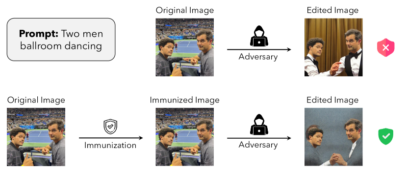
Large diffusion models such as DALLE 2 [RDN+22] and Stable Diffusion [RBL+22] are known for their ability to produce high-quality photorealistic images, and can be used for a variety of image synthesis and editing tasks. However, the ease of use of these models has raised concerns about their potential abuse, e.g., by creating inappropriate or harmful digital content. For example, a malevolent actor might download photos of people posted online and edit them maliciously using an off-the-shelf diffusion model (as in Figure 1 top).
How can we address these concerns? First, it is important to recognize that it is, in some sense, impossible to completely eliminate such malicious image editing. Indeed, even without diffusion models in the picture, malevolent actors can still use tools such as Photoshop to manipulate existing images, or even synthesize fake ones entirely from scratch. The key new problem that large generative models introduce is that these actors can now create realistic edited images with ease, i.e., without the need for specialized skills or expensive equipment. This realization motivates us to ask:
How can we raise the cost of malicious (AI-powered) image manipulation?
In this paper, we put forth an approach that aims to alter the economics of AI-powered image editing. At the core of our approach is the idea of image immunization—that is, making a specific image resistant to AI-powered manipulation by adding a carefully crafted (imperceptible) perturbation to it. This perturbation would disrupt the operation of a diffusion model, forcing the edits it performs to be unrealistic (see Figure 1). In this paradigm, people can thus continue to share their (immunized) images as usual, while getting a layer of protection against undesirable manipulation.
We demonstrate how one can craft such imperceptible perturbations for large-scale diffusion models and show that they can indeed prevent realistic image editing. We then discuss in Section 5 complementary technical and policy components needed to make our approach fully effective and practical.
2 Preliminaries
We start by providing an overview of diffusion models as well as of the key concept we will leverage: adversarial attacks.
2.1 Diffusion Models
Diffusion models have emerged recently as powerful tools for generating realistic images [SWM+15, HJA20]. These models excel especially at generating and editing images using textual prompts, and currently surpass other image generative models such as GANs [GPM+14] in terms of the quality of produced images.
Diffusion process.
At their core, diffusion models employ a stochastic differential process called the diffusion process [SWM+15]. This process allows us to view the task of (approximate) sampling from a distribution of real images as a series of denoising problems. More precisely, given a sample , the diffusion process incrementally adds noise to generate samples for steps, where , and is sampled from a Gaussian distribution333Here, and are the parameters of the distribution . Details are provided in Appendix B.. Note that, as a result, the sample starts to follow a standard normal distribution when . Now, if we reverse this process and are able to sample given , i.e., denoise , we can ultimately generate new samples from . This is done by simply starting from (which corresponds to being sufficiently large), and iteratively denoising these samples for T steps, to produce a new image .
The element we need to implement this process is thus to learn a neural network that “predicts” given the noise added to at each time step . Consequently, this denoising model is trained to minimize the following loss function:
| (1) |
where is sampled uniformly over the time steps. We defer discussion of details to Appendix B and refer the reader to [Wen21] for a more in-depth treatment of diffusion models.
Latent diffusion models (LDMs).
Our focus will be on a specific class of diffusion models called the latent diffusion models (LDMs) [RBL+22]444Our methodology can be adjusted to other diffusion models. Our focus on LDMs is motivated by the fact that all popular open-sourced diffusion models are of this type.. These models apply the diffusion process described above in the latent space instead of the input (image) space. As it turned out, this change enables more efficient training and faster inference, while maintaining high quality generated samples.
Training an LDM is similar to training a standard diffusion model and differs mainly in one aspect. Specifically, to train an LDM, the input image is first mapped to its latent representation , where is a given encoder. The diffusion process then continues as before (just in the latent space) by incrementally adding noise to generate samples for steps, where , and is sampled from a Gaussian distribution. Finally, the denoising network is then learned analogously to as before but, again, now in the latent space, by minimizing the following loss function:
| (2) |
Once the denoising network is trained, the same generative process can be applied as before, starting from a random vector in the latent space, to obtain a latent representation of the (new) generated image. This representation is then decoded into an image , using the corresponding decoder .
Prompt-guided sampling using an LDM.
An LDM by default generates a random sample from the distribution of images it was trained on. However, it turns out one can also guide the sampling using natural language. This can be accomplished by combining the latent representation produced during the diffusion process with the embedding of the user-defined textual prompt .555Conditioning on the text embedding happens at every stage of the generation process. See [RBL+22] for more details. The denoising network is applied to the combined representation for steps, yielding which is then mapped to a new image using the decoder as before.
LDMs capabilities.
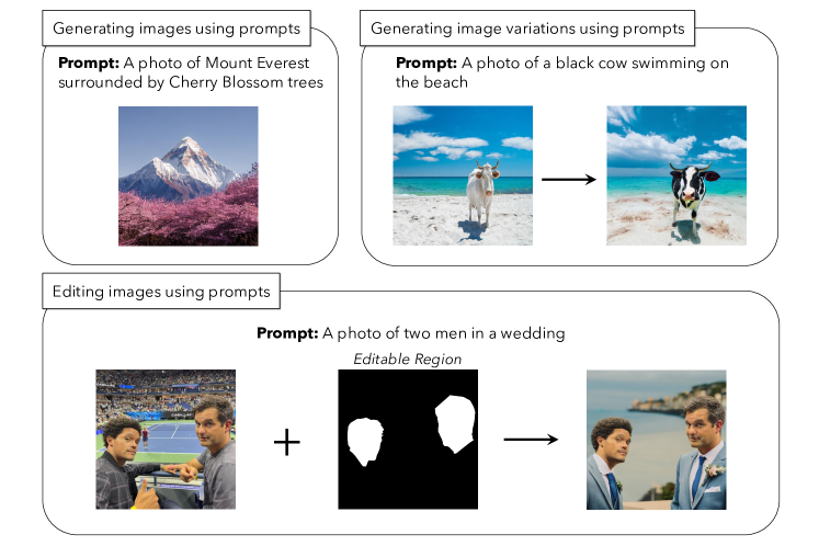
LDMs turn out to be powerful text-guided image generation and editing tools. In particular, LDMs can be used not only for generating images using textual prompts, as described above, but also for generating textual prompt–guided variations of an image or edits of a specific part of an image (see Figure 2). The latter two capabilities (i.e., generation of image variations and image editing) requires a slight modification of the generative process described above. Specifically, to modify or edit a given image , we condition the generative process on this image. That is, instead of applying, as before, our generative process of denoising steps to a random vector in the latent space, we apply it to the latent representation obtained from running the latent diffusion process on our image . To edit only part of the image we additionally condition the process on freezing the parts of the image that were to remain unedited.
2.2 Adversarial Attacks
For a given computer vision model and an image, an adversarial example is an imperceptible perturbation of that image that manipulates the model’s behavior [SZS+14, BCM+13]. In image classification, for example, an adversary can construct an adversarial example for a given image that makes it classified as a specific target label (different from the true label). This construction is achieved by minimizing the loss of a classifier with respect to that image:
| (3) |
Here, is a set of perturbations that are small enough that they are imperceptible—a common choice is to constrain the adversarial example to be close (in distance) to the original image, i.e., . The canonical approach to constructing an adversarial example is to solve the optimization problem (3) via projected gradient descent (PGD) [Nes03, MMS+18].
3 Adversarially Attacking Latent Diffusion Models
We now describe our approach to immunizing images, i.e., making them harder to manipulate using latent diffusion models (LDMs). At the core of our approach is to leverage techniques from the adversarial attacks literature [SZS+14, MMS+18, AMK+21] and add adversarial perturbations (see Section 2.1) to immunize images. Specifically, we present two different methods to execute this strategy (see Figure 3): an encoder attack, and a diffusion attack.
Encoder attack.
Recall that an LDM, when applied to an image, first encodes the image using an encoder into a latent vector representation, which is then used to generate a new image (see Section 2). The key idea behind our encoder attack is now to disrupt this process by forcing the encoder to map the input image to some “bad” representation. To achieve this, we solve the following optimization problem using projected gradient descent (PGD):
| (4) |
where is the image to be immunized, and is some target latent representation (e.g., can be the representation, produced using encoder , of a gray image). Solutions to this optimization problem yield small, imperceptible perturbations which, when added to the original image, result in an (immunized) image that is similar to the (gray) target image from the LDM’s encoder perspective. This, in turn, causes the LDM to generate an irrelevant or unrealistic image. An overview of this attack is shown in Figure 3 (left)666See Algorithm 1 in Appendix for the details of the encoder attack..
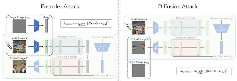
Diffusion attack.
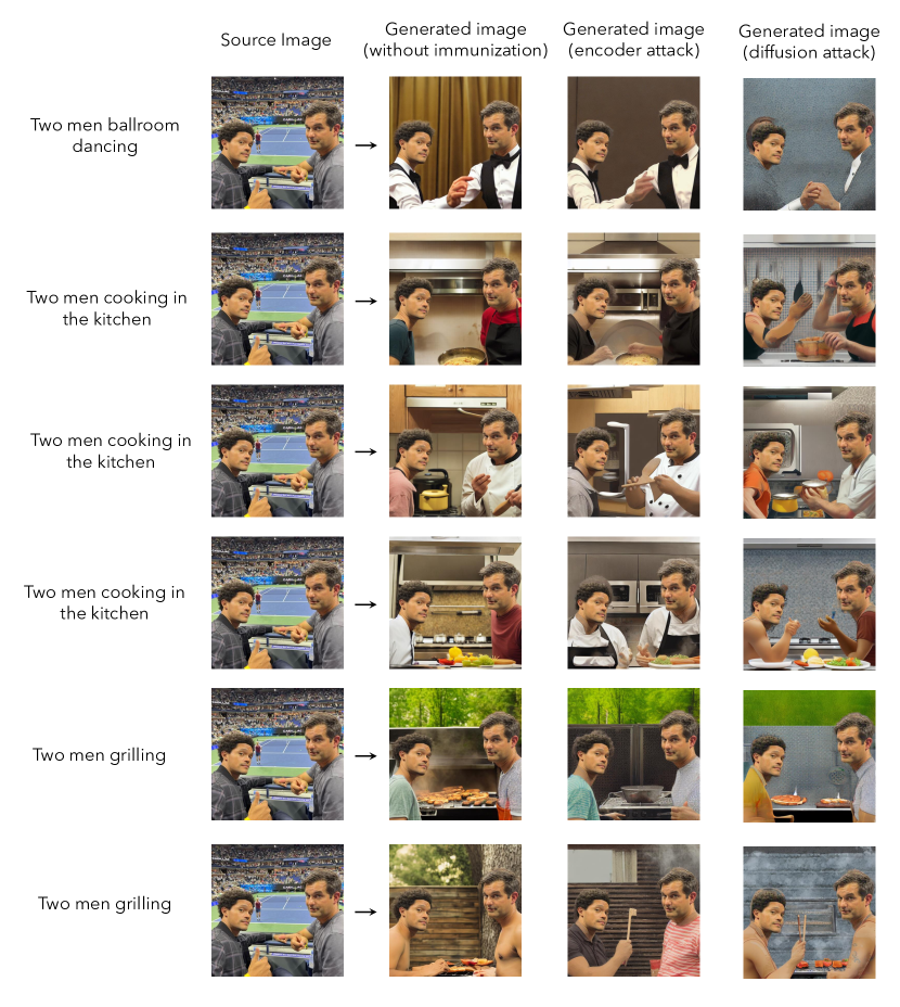
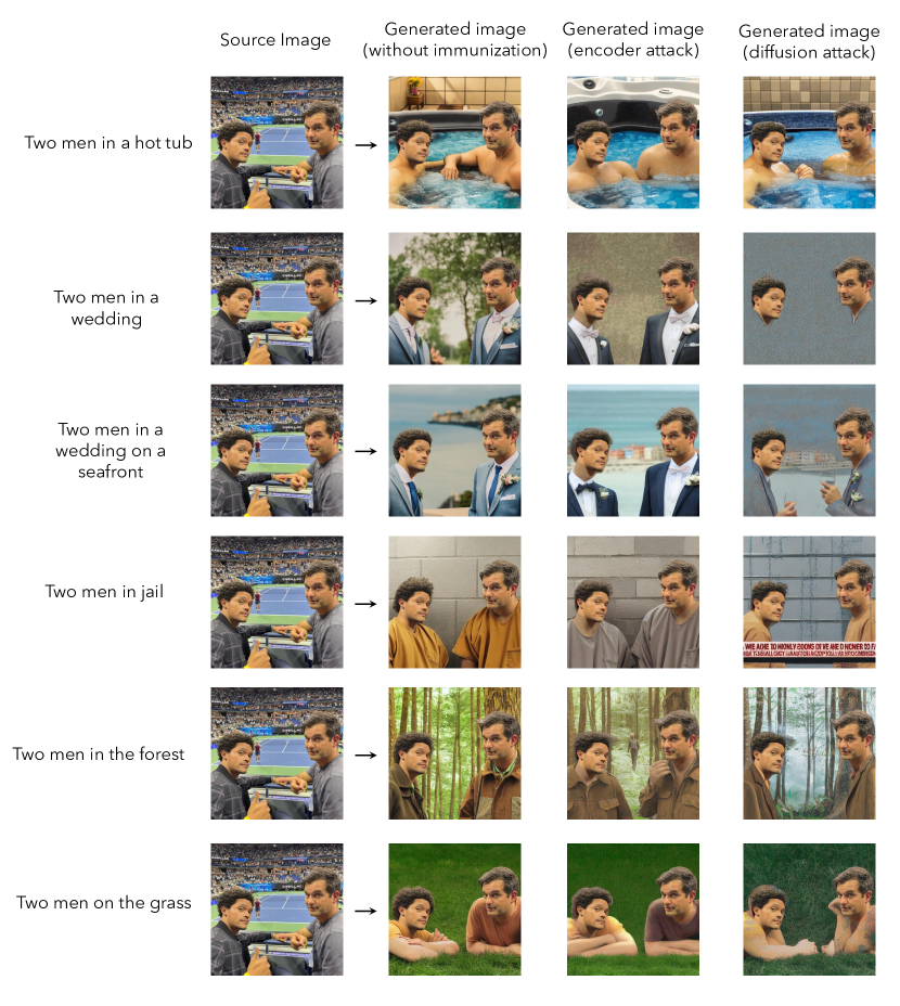
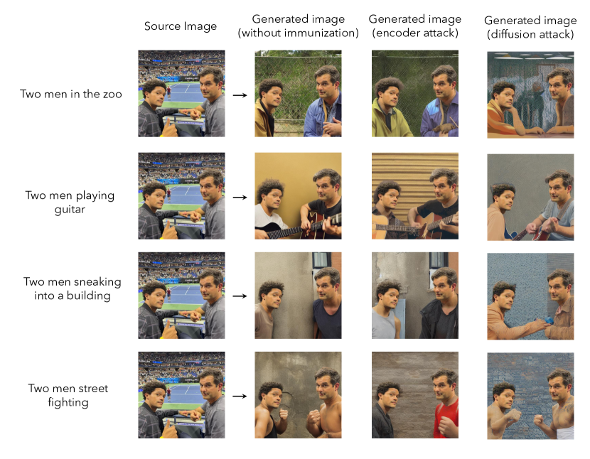
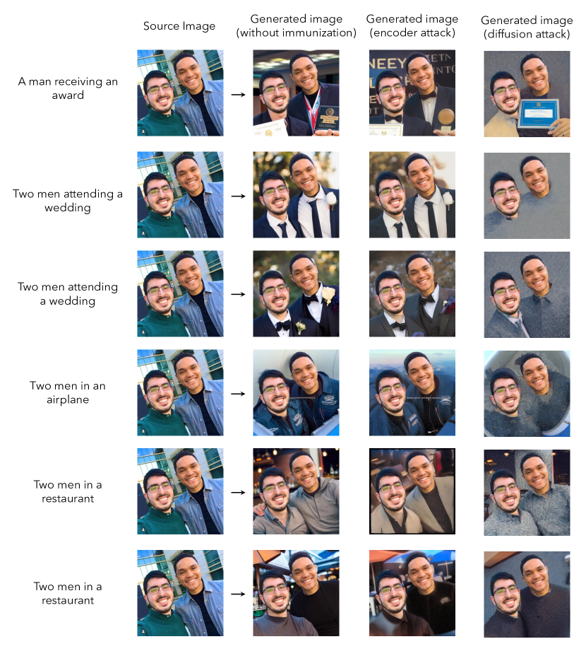
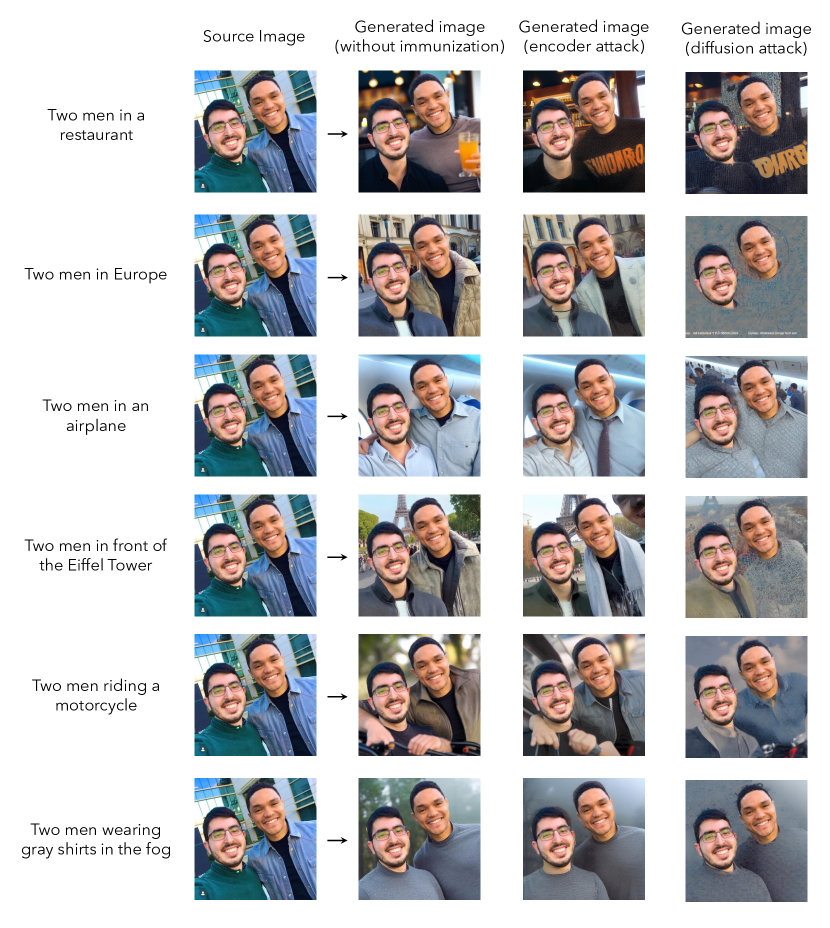
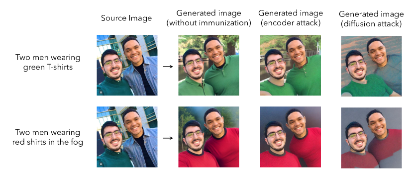
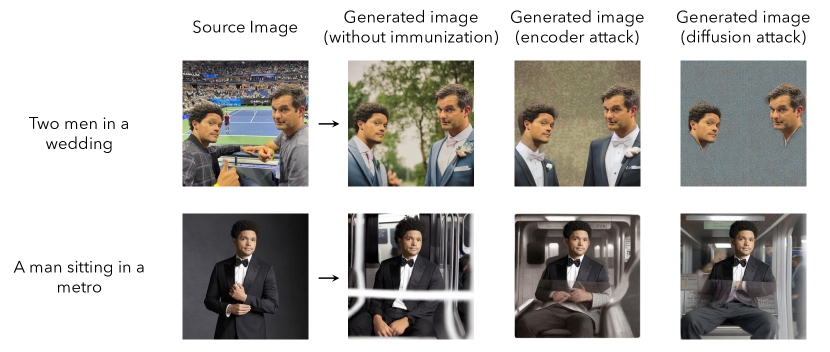
Although the encoder attack is effective at forcing the LDM to generate images that are unrelated to the immunized ones, we still expect the LDM to use the textual prompt. For example, as shown in the encoder attack diagram in Figure 3, editing an immunized image of two men using the prompt “Two men in a wedding” still results in a generated image with two men wearing wedding suits, even if the image will contain some visual artifacts indicating that it has been manipulated. Can we disturb the diffusion process even further so that the diffusion model “ignores” the textual prompt entirely and generates a more obviously manipulated image?
It turns out that we are able to do so by using a more complex attack, one where we target the diffusion process itself instead of just the encoder. In this attack, we perturb the input image so that the final image generated by the LDM is a specific target image (e.g., random noise or gray image). Specifically, we generate an adversarial perturbation by solving the following optimization problem (again via PGD):
| (5) |
Above, is the LDM, is the image to be immunized, and is the target image to be generated. An overview of this attack is depicted in Figure 3 (right)777See Algorithm 2 in Appendix for the details of the diffusion attack.. As we already mentioned, this attack targets the full diffusion process (which includes the text prompt conditioning), and tries to nullify not only the effect of the immunized image, but also that of the text prompt itself. Indeed, in our example (see Figure 3 (right)) no wedding suits appear in the edited image whatsoever.
It is worth noting that this approach, although more powerful than the encoder attack, is harder to execute. Indeed, to solve the above problem (5) using PGD, one needs to backpropagate through the full diffusion process (which, as we recall from Section 2.1, includes repeated application of the denoising step). This causes memory issues even on the largest GPU we used888We used an A100 with 40 GB memory.. To address this challenge, we backpropagate through only a few steps of the diffusion process, instead of the full process, while achieving adversarial perturbations that are still effective. We defer details of our attacks to Appendix A.
4 Results
In this section, we examine the effectiveness of our proposed immunization method.
Setup.
We focus on the Stable Diffusion Model (SDM) v1.5 [RBL+22], though our methods can be applied to other diffusion models too. In each of the following experiments, we aim to disrupt the performance of SDM by adding imperceptible noise (using either of our proposed attacks)—i.e., applying our immunization procedure—to a variety of images. The goal is to force the model to generate images that are unrealistic and unrelated to the original (immunized) image. We evaluate the performance of our method both qualitatively (by visually inspecting the generated images) and quantitatively (by examining the image quality using standard metrics). We defer further experimental details to Appendix A.
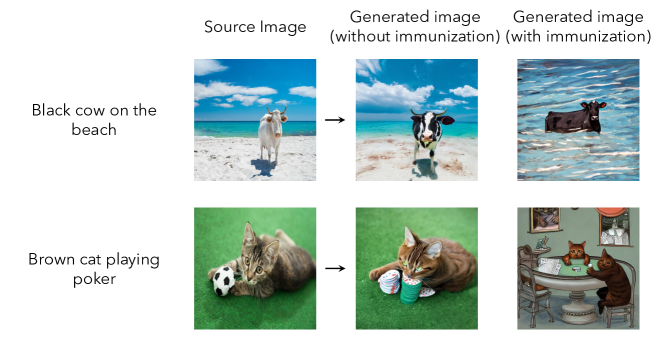
4.1 Qualitative Results
Immunizing against generating image variations.
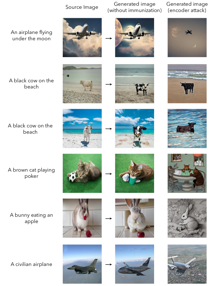
We first assess whether we can disrupt the SDM’s ability to generate realistic variations of an image based on a given textual prompt. For example, given an image of a white cow on the beach and a prompt of “black cow on the beach”, the SDM should generate a realistic image of a black cow on the beach that looks similar to the original one (cf. Figure 4). Indeed, the SDM is able to generate such images. However, when we immunize the original images (using the encoder attack), the SDM fails to generate a realistic variation—see Figure 4.
Immunizing against image editing.
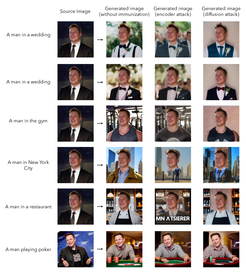
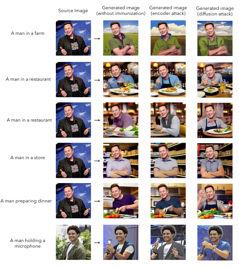
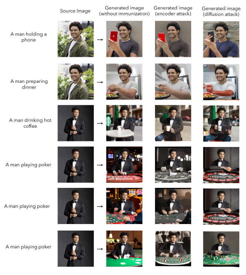
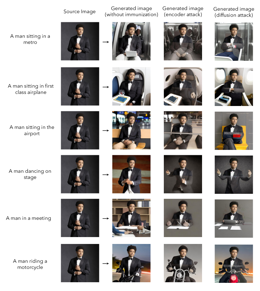
Now we consider the more challenging task of disrupting the ability of SDMs to edit images using textual prompts. The process of editing an image using an SDM involves inputting the image, a mask indicating which parts of the image should be edited, and a text prompt guiding how the rest of the image should be manipulated. The SDM then generates an edited version based on that prompt. An example can be seen in Figure 2, where an image of two men watching a tennis game is transformed to resemble a wedding photo. This corresponded to inputting the original image, a binary mask excluding from editing only the men’s heads, and the prompt “A photo of two men in a wedding.” However, when the image is immunized (using either encoder or diffusion attacks), the SDM is unable to produce realistic image edits (cf. Figure 5). Furthermore, the diffusion attack results in more unrealistic images than the encoder attack.
| Method | FID | PR | SSIM | PSNR | VIFp | FSIM |
|---|---|---|---|---|---|---|
| Immunization baseline (Random noise) | 82.57 | 1.00 | ||||
| Immunization (Encoder attack) | 130.6 | 0.95 | ||||
| Immunization (Diffusion attack) | 167.6 | 0.87 |
4.2 Quantitative Results
Image quality metrics.
Figures 4 and 5 indicate that, as desired, edits of immunized images are noticeably different from those of non-immunized images. To quantify this difference, we generate 60 different edits of a variety of images using different prompts, and then compute several metrics capturing the similarity between resulting edits of immunized versus non-immunized images999We use the implementations provided in: https://github.com/photosynthesis-team/piq.: FID [HRU+17], PR [SBL+18], SSIM [WBS+04], PSNR, VIFp [SB06], and FSIM [ZZM+11]101010We report additional metrics in Appendix C.1.. The better our immunization method is, the less similar the edits of immunized images are to those of non-immunized images.
The similarity scores, shown in Table 6, indicate that applying either of our immunization methods (encoder or diffusion attacks) indeed yields edits that are different from those of non-immunized images (since, for example, FID is far from zero for both of these methods). As a baseline, we consider a naive immunization method that adds uniform random noise (of the same intensity as the perturbations used in our proposed immunization method). This method, as we verified, is not effective at disrupting the SDM, and yields edits almost identical to those of non immunized images. Indeed, in Table 6, the similarity scores of this baseline indicate closer edits to non-immunized images compared to both of our attacks.
Image-prompt similarity.
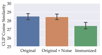
To further evaluate the quality of the generated/edited images after immunization (using diffusion attack), we measure the similarity between the edited images and the textual prompt used to guide this edit, with and without immunization. The fact that the SDM uses the textual prompt to guide the generation of an image indicates that the similarity between the generated image and the prompt should be high in the case of no immunization. However, after immunization (using the diffusion attack), the similarity should be low, since the immunization process disrupts the full diffusion process, and forces the diffusion model to ignore the prompt during generation. We use the same 60 edits as in our previous experiment, and we extract—using a pretrained CLIP model [RKH+21]—the visual embeddings of these images and the textual prompts used to generate them. We then compute the cosine similarity between these two embeddings. As show in Figure 7, the immunization process decreases the similarity between the generated images and the textual prompts to generated them, as expected.
5 A Techno-Policy Approach to Mitigation of AI-Powered Editing
In the previous sections we have developed an immunization procedure that, when applied to an image, protects the immunized version of that image from realistic manipulation by a given diffusion model. Our immunization procedure has, however, certain important limitations. We now discuss these limitations as well as a combination of technical and policy remedies needed to obtain a fully effective approach to raising the cost of malicious AI-powered image manipulation.
(Lack of) robustness to transformations.
One of the limitations of our immunization method is that the adversarial perturbation that it relies on may be ineffective after the immunized image is subjected to image transformations and noise purification techniques. For instance, malicious actors could attempt to remove the disruptive effect of that perturbation by cropping the image, adding filters to it, applying a rotation, or other means. This problem can be addressed, however, by leveraging a long line of research on creating robust adversarial perturbations, i.e., adversarial perturbations that can withstand a broad range of image modifications and noise manipulations [EEF+18, KGB16, AEI+18, BMR+18].
Forward-compatibility of the immunization.
While the immunizing adversarial perturbations we produce might be effective at disrupting the current generation of diffusion-based generative models, they are not guaranteed to be effective against the future versions of these models. Indeed, one could hope to rely here on the so-called transferability of adversarial perturbations [PMG16, LCL+17], but no perturbation will be perfectly transferable.
To truly address this limitation, we thus need to go beyond purely technical methods and encourage—or compel—via policy means a collaboration between organizations that develop large diffusion models, end-users, as well as data hosting and dissemination platforms. Specifically, this collaboration would involve the developers providing APIs that allow the users and platforms to immunize their images against manipulation by the diffusion models the developers create. Importantly, these APIs should guarantee “forward compatibility”, i.e., effectiveness of the offered immunization against models developed in the future. This can be accomplished by planting, when training such future models, the current immunizing adversarial perturbations as backdoors. (Observe that our immunization approach can provide post-hoc “backward compatibility” too. That is, one can create immunizing adversarial perturbations that are effective for models that were already released.)
It is important to point out that we are leveraging here an incentive alignment that is fundamentally different to the one present in more typical applications of adversarial perturbations and backdoor attacks. In particular, the “attackers” here—that is, the parties that create the adversarial perturbations/execute the backdoor attack—are the same parties that develop the models being attacked. This crucial difference is, in particular, exactly what helps remedy the forward compatibility challenges that turns out to be crippling, e.g., in the context of “unlearnable” images creation (i.e., creation of images that are immune to being leveraged by, e.g., facial recognition models) [RHC+21].
6 Related Work
Data misuse after model training.
Recent advances in ML-powered image generation and editing have raised concerns about the potential misuse of personal data for generating fake images. This issue arose first in the context of the development of generative adversarial networks (GANs) for image generation and editing [GPM+14, MO14, SGZ+16, IZZ+17, ZPI+17, ZXL+17, KAL+18, BDS19, KLA19], and led to research on methods for defending against such manipulation, such as attacking the GAN itself [RAS20, RBS20, SZZ+21]. This problem became exacerbated recently with the advent of (publicly available) diffusion models [RBL+22, RDN+22]. Indeed, one can now easily describe in text how one wants to manipulate an image, and immediately get the result of an impressive quality (see Figure 2) that significantly outperforms previous methods, such as GANs.
Deepfake detection.
A line of work related to ours aims to detect fake images rather than prevent their generation. Deepfake detection methods include analyzing the consistency of facial expressions and identifying patterns or artifacts in the image that may indicate manipulation, and training machine learning models to recognize fake images [KM18, ANY+18, NNN+19, ML21, RCV+19, DKP+19, LBZ+20, LYS+20, BCM+21]. While some deepfake detection methods are more effective than others, no single method is foolproof. A potential way to mitigate this shortcoming could involve development of so-called watermarking methods [CKL+97, NHZ+22]. These methods aim to ensure that it is easy to detect that a given output has been produced using a generative model—such watermarking approaches have been recently developed for a related context of large language models [KGW+23]. Still, neither deepfake detection nor watermarking methods could protect images from being manipulated in the first place. A manipulated image can hence cause harm before being flagged as fake. Also, given that our work is complementary to deepfake detection and watermarking methods, it could, in principle, be combined with them.
Data misuse during model training.
The abundance of readily available data on the Internet has played a significant role in recent breakthroughs in deep learning, but has also raised concerns about the potential misuse of such data when training models. Therefore, there has been an increasing interest in protection against unauthorized data exploitation, e.g., by designing unlearnable examples [HME+21, FHL+21]. These methods propose adding imperceptible backdoor signals to user data before uploading it online, so as to prevent models from fruitfully utilizing this data. However, as pointed out by [RHC+21], these methods can be circumvented, often simply by waiting until subsequently developed models can avoid being fooled by the planted backdoor signal.
7 Conclusion
In this paper, we presented a method for raising the difficulty of using diffusion models for malicious image manipulation. Our method involves “immunizing” images through addition imperceptible adversarial perturbations. These added perturbations disrupt the inner workings of the targeted diffusion model and thus prevent it from producing realistic modifications of the immunized images.
We also discussed the complementary policy component that will be needed to make our approach fully effective. This component involves ensuring cooperation of the organizations developing diffusion-based generative models in provisioning APIs that allow users to immunize their images to manipulation by such models (and the future versions of thereof).
8 Acknowledgements
Work supported in part by the NSF grants CNS-1815221 and DMS-2134108, and Open Philanthropy. This material is based upon work supported by the Defense Advanced Research Projects Agency (DARPA) under Contract No. HR001120C0015. Work partially done on the MIT Supercloud compute cluster [RKB+18].
References
- [AEI+18] Anish Athalye, Logan Engstrom, Andrew Ilyas and Kevin Kwok “Synthesizing Robust Adversarial Examples” In International Conference on Machine Learning (ICML), 2018
- [AMK+21] Naveed Akhtar, Ajmal Mian, Navid Kardan and Mubarak Shah “Threat of Adversarial Attacks on Deep Learning in Computer Vision: Survey” In arXiV, 2021
- [ANY+18] Darius Afchar, Vincent Nozick, Junichi Yamagishi and Isao Echizen “Mesonet: a compact facial video forgery detection network” In 2018 IEEE international workshop on information forensics and security (WIFS), 2018, pp. 1–7 IEEE
- [BCM+13] Battista Biggio, Igino Corona, Davide Maiorca, Blaine Nelson, Nedim Šrndić, Pavel Laskov, Giorgio Giacinto and Fabio Roli “Evasion attacks against machine learning at test time” In Joint European conference on machine learning and knowledge discovery in databases (ECML-KDD), 2013
- [BCM+21] Nicolo Bonettini, Edoardo Daniele Cannas, Sara Mandelli, Luca Bondi, Paolo Bestagini and Stefano Tubaro “Video face manipulation detection through ensemble of cnns” In 2020 25th international conference on pattern recognition (ICPR), 2021, pp. 5012–5019 IEEE
- [BDS19] Andrew Brock, Jeff Donahue and Karen Simonyan “Large Scale GAN Training for High Fidelity Natural Image Synthesis” In International Conference on Learning Representations (ICLR), 2019
- [BMR+18] Tom B. Brown, Dandelion Mané, Aurko Roy, Martín Abadi and Justin Gilmer “Adversarial Patch”, 2018 arXiv:1712.09665 [cs.CV]
- [BSM+15] Amnon Balanov, Arik Schwartz, Yair Moshe and Nimrod Peleg “Image quality assessment based on DCT subband similarity” In IEEE International Conference on Image Processing (ICIP), 2015
- [CKL+97] Ingemar J Cox, Joe Kilian, F Thomson Leighton and Talal Shamoon “Secure spread spectrum watermarking for multimedia” In IEEE transactions on image processing 6.12 IEEE, 1997, pp. 1673–1687
- [DKP+19] Ricard Durall, Margret Keuper, Franz-Josef Pfreundt and Janis Keuper “Unmasking deepfakes with simple features” In arXiv preprint arXiv:1911.00686, 2019
- [EEF+18] Kevin Eykholt, Ivan Evtimov, Earlence Fernandes, Bo Li, Amir Rahmati, Florian Tramer, Atul Prakash, Tadayoshi Kohno and Dawn Song “Physical Adversarial Examples for Object Detectors” In CoRR, 2018
- [FHL+21] Shaopeng Fu, Fengxiang He, Yang Liu, Li Shen and Dacheng Tao “Robust unlearnable examples: Protecting data privacy against adversarial learning” In International Conference on Learning Representations, 2021
- [GPM+14] Ian Goodfellow, Jean Pouget-Abadie, Mehdi Mirza, Bing Xu, David Warde-Farley, Sherjil Ozair, Aaron Courville and Yoshua Bengio “Generative adversarial nets” In neural information processing systems (NeurIPS), 2014
- [HJA20] Jonathan Ho, Ajay Jain and Pieter Abbeel “Denoising Diffusion Probabilistic Models” In Neural Information Processing Systems (NeurIPS), 2020
- [HME+21] Hanxun Huang, Xingjun Ma, Sarah Monazam Erfani, James Bailey and Yisen Wang “Unlearnable Examples: Making Personal Data Unexploitable” In ICLR, 2021
- [HRU+17] Martin Heusel, Hubert Ramsauer, Thomas Unterthiner, Bernhard Nessler and Sepp Hochreiter “Gans trained by a two time-scale update rule converge to a local nash equilibrium” In Neural Information Processing Systems (NeurIPS), 2017
- [IZZ+17] Phillip Isola, Jun-Yan Zhu, Tinghui Zhou and Alexei A Efros “Image-to-image translation with conditional adversarial networks” In conference on computer vision and pattern recognition (CVPR), 2017
- [KAL+18] Tero Karras, Timo Aila, Samuli Laine and Jaakko Lehtinen “Progressive Growing of GANs for Improved Quality, Stability, and Variation” In International Conference on Learning Representations, 2018
- [KGB16] Alexey Kurakin, Ian Goodfellow and Samy Bengio “Adversarial examples in the physical world” In arXiv preprint arXiv:1607.02533, 2016
- [KGW+23] John Kirchenbauer, Jonas Geiping, Yuxin Wen, Jonathan Katz, Ian Miers and Tom Goldstein “A Watermark for Large Language Models”, 2023
- [KLA19] Tero Karras, Samuli Laine and Timo Aila “A style-based generator architecture for generative adversarial networks” In Proceedings of the IEEE/CVF conference on computer vision and pattern recognition, 2019, pp. 4401–4410
- [KM18] Pavel Korshunov and Sébastien Marcel “Deepfakes: a new threat to face recognition? assessment and detection” In arXiv preprint arXiv:1812.08685, 2018
- [LBZ+20] Lingzhi Li, Jianmin Bao, Ting Zhang, Hao Yang, Dong Chen, Fang Wen and Baining Guo “Face x-ray for more general face forgery detection” In Proceedings of the IEEE/CVF conference on computer vision and pattern recognition, 2020, pp. 5001–5010
- [LCL+17] Yanpei Liu, Xinyun Chen, Chang Liu and Dawn Song “Delving into Transferable Adversarial Examples and Black-box Attacks” In International Conference on Learning Representations (ICLR), 2017
- [LYS+20] Yuezun Li, Xin Yang, Pu Sun, Honggang Qi and Siwei Lyu “Celeb-df: A large-scale challenging dataset for deepfake forensics” In Proceedings of the IEEE/CVF conference on computer vision and pattern recognition, 2020, pp. 3207–3216
- [ML21] Yisroel Mirsky and Wenke Lee “The creation and detection of deepfakes: A survey” In ACM Computing Surveys (CSUR) 54.1 ACM New York, NY, USA, 2021, pp. 1–41
- [MMS+18] Aleksander Madry, Aleksandar Makelov, Ludwig Schmidt, Dimitris Tsipras and Adrian Vladu “Towards deep learning models resistant to adversarial attacks” In International Conference on Learning Representations (ICLR), 2018
- [MO14] Mehdi Mirza and Simon Osindero “Conditional generative adversarial nets” In arXiv preprint arXiv:1411.1784, 2014
- [Nes03] Yurii Nesterov “Introductory Lectures on Convex Optimization”, 2003
- [NHZ+22] Paarth Neekhara, Shehzeen Hussain, Xinqiao Zhang, Ke Huang, Julian McAuley and Farinaz Koushanfar “FaceSigns: semi-fragile neural watermarks for media authentication and countering deepfakes” In arXiv preprint arXiv:2204.01960, 2022
- [NNN+19] Thanh Thi Nguyen, Cuong M. Nguyen, Dung Tien Nguyen, Duc Thanh Nguyen and Saeid Nahavandi “Deep Learning for Deepfakes Creation and Detection” In arXiV, 2019
- [PMG16] Nicolas Papernot, Patrick McDaniel and Ian Goodfellow “Transferability in Machine Learning: from Phenomena to Black-box Attacks using Adversarial Samples” In ArXiv preprint arXiv:1605.07277, 2016
- [RAS20] Nataniel Ruiz, Sarah Adel Bargal and Stan Sclaroff “Disrupting Deepfakes: Adversarial Attacks Against Conditional Image Translation Networks and Facial Manipulation Systems” In arXiv, 2020
- [RBK+18] Rafael Reisenhofer, Sebastian Bosse, Gitta Kutyniok and Thomas Wiegand “A Haar wavelet-based perceptual similarity index for image quality assessment” In Signal Processing: Image Communication, 2018
- [RBL+22] Robin Rombach, Andreas Blattmann, Dominik Lorenz, Patrick Esser and Björn Ommer “High-resolution image synthesis with latent diffusion models” In Proceedings of the IEEE/CVF Conference on Computer Vision and Pattern Recognition, 2022, pp. 10684–10695
- [RBS20] Nataniel Ruiz, Sarah Bargal and Stan Sclaroff “Protecting Against Image Translation Deepfakes by Leaking Universal Perturbations from Black-Box Neural Networks” In arXiV, 2020
- [RCV+19] Andreas Rossler, Davide Cozzolino, Luisa Verdoliva, Christian Riess, Justus Thies and Matthias Nießner “Faceforensics++: Learning to detect manipulated facial images” In Proceedings of the IEEE/CVF international conference on computer vision, 2019, pp. 1–11
- [RDN+22] Aditya Ramesh, Prafulla Dhariwal, Alex Nichol, Casey Chu and Mark Chen “Hierarchical text-conditional image generation with clip latents” In arXiv preprint arXiv:2204.06125, 2022
- [RHC+21] Evani Radiya-Dixit, Sanghyun Hong, Nicholas Carlini and Florian Tramèr “Data Poisoning Won’t Save You From Facial Recognition” arXiv, 2021
- [RKB+18] Albert Reuther, Jeremy Kepner, Chansup Byun, Siddharth Samsi, William Arcand, David Bestor, Bill Bergeron, Vijay Gadepally, Michael Houle, Matthew Hubbell, Michael Jones, Anna Klein, Lauren Milechin, Julia Mullen, Andrew Prout, Antonio Rosa, Charles Yee and Peter Michaleas “Interactive supercomputing on 40,000 cores for machine learning and data analysis” In 2018 IEEE High Performance extreme Computing Conference (HPEC), 2018, pp. 1–6 IEEE
- [RKH+21] Alec Radford, Jong Wook Kim, Chris Hallacy, Aditya Ramesh, Gabriel Goh, Sandhini Agarwal, Girish Sastry, Amanda Askell, Pamela Mishkin and Jack Clark “Learning transferable visual models from natural language supervision” In arXiv preprint arXiv:2103.00020, 2021
- [SB06] H.R. Sheikh and A.C. Bovik “Image information and visual quality” In IEEE Transactions on Image Processing, 2006
- [SBL+18] Mehdi S.. Sajjadi, Olivier Bachem, Mario Lučić, Olivier Bousquet and Sylvain Gelly “Assessing Generative Models via Precision and Recall” In Advances in Neural Information Processing Systems (NeurIPS), 2018
- [SGZ+16] Tim Salimans, Ian Goodfellow, Wojciech Zaremba, Vicki Cheung, Alec Radford and Xi Chen “Improved techniques for training gans” In neural information processing systems (NeurIPS), 2016
- [SWM+15] Jascha Sohl-Dickstein, Eric A. Weiss, Niru Maheswaranathan and Surya Ganguli “Deep Unsupervised Learning Using Nonequilibrium Thermodynamics” In International Conference on Machine Learning, 2015
- [SZS+14] Christian Szegedy, Wojciech Zaremba, Ilya Sutskever, Joan Bruna, Dumitru Erhan, Ian Goodfellow and Rob Fergus “Intriguing properties of neural networks” In International Conference on Learning Representations (ICLR), 2014
- [SZZ+21] Hui Sun, Tianqing Zhu, Zhiqiu Zhang, Dawei Jin Xiong and Wanlei Zhou “Adversarial attacks against deep generative models on data: a survey” In arXiv preprint arXiv:2112.00247, 2021
- [WBS+04] Zhou Wang, A.C. Bovik, H.R. Sheikh and E.P. Simoncelli “Image quality assessment: from error visibility to structural similarity” In IEEE Transactions on Image Processing, 2004
- [Wen21] Lilian Weng “What are diffusion models?” In lilianweng.github.io, 2021 URL: https://lilianweng.github.io/posts/2021-07-11-diffusion-models/
- [XZM+14] Wufeng Xue, Lei Zhang, Xuanqin Mou and Alan C. Bovik “Gradient Magnitude Similarity Deviation: A Highly Efficient Perceptual Image Quality Index” In IEEE Transactions on Image Processing, 2014
- [ZL12] Lin Zhang and Hongyu Li “SR-SIM: A fast and high performance IQA index based on spectral residual” In 2012 19th IEEE International Conference on Image Processing, 2012
- [ZPI+17] Jun-Yan Zhu, Taesung Park, Phillip Isola and Alexei A Efros “Unpaired image-to-image translation using cycle-consistent adversarial networks” In international conference on computer vision(ICCV), 2017
- [ZSL14] Lin Zhang, Ying Shen and Hongyu Li “VSI: A Visual Saliency-Induced Index for Perceptual Image Quality Assessment” In IEEE Transactions on Image Processing, 2014
- [ZXL+17] Han Zhang, Tao Xu, Hongsheng Li, Shaoting Zhang, Xiaogang Wang, Xiaolei Huang and Dimitris N Metaxas “Stackgan: Text to photo-realistic image synthesis with stacked generative adversarial networks” In Proceedings of the IEEE international conference on computer vision, 2017, pp. 5907–5915
- [ZZM+11] Lin Zhang, Lei Zhang, Xuanqin Mou and David Zhang “FSIM: A Feature Similarity Index for Image Quality Assessment” In IEEE Transactions on Image Processing, 2011
Appendix A Experimental Setup
A.1 Details of the diffusion model we used
In this paper, we used the open-source stable diffusion model hosted on the Hugging Face111111This model is available on: https://huggingface.co/runwayml/stable-diffusion-v1-5.. We use the hyperparameters presented in Table 8 to generated images from this model. For a given image on which we want to test our immunization method, we first search for a good random seed that leads to a realistic modification of the image given some textual prompt. Then we use the same seed when editing the immunized version of the same image using the diffusion model. This ensures that the immunized image is modified in the same way as the original image, and that the resulting non-realistic edits are due to immunization and not to random seed.
| height | width | guidance_scale | num_inference_steps | eta |
|---|---|---|---|---|
| 512 | 512 | 7.5 | 100 | 1 |
A.2 Our attacks details
Throughout the paper, we use two different attacks: an encoder attack and a diffusion attack. These attacks are described in the main paper, and are summarized here in Algorithm 1 and Algorithm 2, respectively. For both of the attacks, we use the same set of hyperparameters shown in Table 9. The choice of was such that it is the large enough to disturb the image, but small enough to not be noticeable by the human eye.
| Norm | step size | number of steps | |
|---|---|---|---|
| 16/255 | 2/255 | 200 |
Appendix B Extended Background for Diffusion Models
Overview of the diffusion process.
At their heart, diffusion models leverage a statistical concept: the diffusion process [SWM+15, HJA20]. Given a sample from a distribution of real images , the diffusion process works in two steps: a forward step and a backward step. During the forward step, Gaussian noise is added to the sample over time steps, to generate increasingly noisier versions of the original sample , until the sample is equivalent to an isotropic Gaussian distribution. During the backward step, the goal is to reconstruct the original sample by iteratively denoising the noised samples . The power of the diffusion models stems from the ability to learn the backward process using neural networks. This allows to generate new samples from the distribution by first generating a random Gaussian sample, and then passing it through the “neural” backward step.
Forward process.
During the forward step, Gaussian noise is iteratively added to the original sample . The forward process is assumed to follow a Markov chain, i.e. the sample at time step depends only on the sample at the previous time step. Furthermore, the variance added at a time step is controlled by a schedule of variances 121212The values of and from the main paper correspond to and .
| (6) |
Backward process.
At the end of the forward step, the sample looks as if it is sampled from an isotropic Gaussian . Starting from this sample, the goal is to recover by iteratively removing the noise using neural networks. The joint distribution is referred to as the reverse process, and is also assumed to be a Markov chain.
| (7) |
Training a diffusion model.
At its heart, diffusion models are trained in a way similar to Variational Autoencoders, i.e. by optimizing a variational lower bound. Additional tricks are employed to make the process faster. For an extensive derivation, refer to [Wen21].
| (8) |
Latent Diffusion Models (LDMs).
In this paper, we focus on a specific class of diffusion models, namely LDMs, which was proposed in [RBL+22] as a model that applies the diffusion process described above in a latent space instead of the image space. This enables efficient training and inference of diffusion models.
To train an LDM, the input image is first mapped to a latent representation , where is an image encoder. This input representation is then passed to the diffusion process to obtain a denoised . The generated image is then obtained by decoding using a decoder , i.e. .
Appendix C Additional Results
C.1 Additional quantitative results
We presented in Section 4 several metrics to assess the similarity between the images generated with and without immunization. Here, we report in Table 10 additional metrics to evaluate this: SR-SIM [ZL12], GMSD [XZM+14], VSI [ZSL14], DSS [BSM+15], and HaarPSI [RBK+18]. Similarly, we indicate for each metric whether a higher value corresponds to higher similarity (using ), or contrariwise (using ). We again observe that applying the encoder attack already decreases the similarity between the generated images with and without immunization, and applying the diffusion attack further decreases the similarity.
| Method | SR-SIM | GMSD | VSI | DSS | HaarPSI |
|---|---|---|---|---|---|
| Immunization baseline (Random noise) | |||||
| Immunization (Encoder attack) | |||||
| Immunization (Diffusion attack) |
C.2 Generating Image Variations using Textual Prompts
C.3 Image Editing via Inpainting
