A Convex Hull Cheapest Insertion Heuristic for the Non-Euclidean TSP

Abstract

The convex hull cheapest insertion heuristic is known to generate good solutions to the Traveling Salesperson Problem in Euclidean spaces, but it has not been extended to the non-Euclidean case. To address the difficulty of dealing with obstacles in the non-Euclidean space, the proposed adaptation uses multidimensional scaling to first approximate these points in a Euclidean space, thereby enabling the generation of the convex hull that initializes the algorithm. To evaluate the proposed algorithm, the TSPLIB benchmark data-set is modified by adding impassable separators that produce non-Euclidean spaces. The algorithm is demonstrated to outperform the commonly used Nearest Neighbor algorithm in 96% of the cases studied.

1 Introduction

The Traveling Salesperson Problem (TSP) involves finding the shortest possible tour that visits a set of locations exactly once before returning to the starting location. In contrast to TSPs in Euclidean spaces, the non-Euclidean TSP includes obstacles in the environment, or a cost function that is not simply the pairwise Euclidean distance between locations [1]. For example, if the cost to be minimized is the time spent traveling between locations in a city, the optimal tour is dependent on the available road infrastructure that causes path deviations from the straight-line path between locations,the speed limits, and the number of stops or turns to be taken [2].

The non-Euclidean TSP has not been studied as rigorously in literature as their Euclidean counterparts, and a common approach is to either neglect obstacles, or to replace the non-Euclidean cost function with Euclidean distances [3]. This approximation is not always acceptable, especially when obstacles contribute to significant deviations from the straight line path, for example, in the context of robotic material handling operations in intra-factory logistics or warehouses [4, 5]. When the cost being minimized is not simply the Euclidean distance between locations, using methods developed for Euclidean TSPs results in sub-optimal solutions [6].

When the number of locations to be visited is large, exact methods for computing the optimal solution to TSPs are intractable due to their $\mathcal{NP}$-hard nature [7, 8, 9]. When TSP solutions have to be found quickly, heuristics that rapidly find reasonably good solutions are typically used [10, 11, 12]. They are also used to provide solutions that act as upper bounds or as a warm start when initializing exact methods for faster convergence to the optimal solution [13, 14]. However, effective heuristics for the non-Euclidean TSP have been neglected in literature [6, 15], and the simple Nearest Neighbor (NN) greedy heuristic is commonly used [16, 17, 18, 19, 20].

The Convex Hull Cheapest Insertion (CHCI) heuristic has been shown to produce superior solutions to the NN heuristic in most Euclidean test instances [21, 22]. The CHCI heuristic is initiated by a subtour created from the convex hull of locations, and its interior points are then progressively incorporated to the subtour in increasing order of insertion cost, until the complete tour is obtained. The initiation of the candidate subtour with the convex hull of the TSP points is advantageous in generating good solutions because points on the boundary of the convex hull are visited in the same cyclic order as they appear in the optimal Euclidean TSP tour [23, 24, 25]. However, the CHCI heuristic has not been adapted to the non-Euclidean TSP.

The contribution of this paper is the extension of the Euclidean CHCI algorithm to the non-Euclidean TSP, motivated by the expected reduction in tour cost when compared to the NN heuristic. This is achieved by first applying multidimensional scaling (MDS) to find the set of points in a projected Euclidean space whose pairwise distances approximate the non-Euclidean pairwise cost. The points on the boundary of their convex hull are used to initiate a sub-tour onto which the remaining points are added in increasing order of their true non-Euclidean insertion cost. While MDS has recently been applied to the non-Euclidean TSP for tour length estimation, local clustering, and to understand human cognition [26, 27, 28], the use of MDS to initiate the CHCI heuristic for the non-Euclidean TSP is a novel approach. The performance of the proposed algorithm is compared with the NN heuristic on modified TSPLIB benchmark instances [29], showing experimentally that the ACHCI outperforms the NN heuristic in 96% of the cases studied.

2 Non-Euclidean TSP

Consider a complete directed graph represented by $\mathcal{G}:=(V,A)$ where $V$ is the set of locations or nodes, and the directed arc set $A:=\{(v_{i},v_{j})|v_{i},v_{j}\in V,\forall i\neq j\}$ connects every ordered pair of distinct nodes in $V$. A cost function $c:A\rightarrow\mathbb{R}^{+}$ defines the metric to be minimized, and each arc $(v_{i},v_{j})\in A$ is associated with a defined cost $c(v_{i},v_{j})\in\mathbb{R}^{+}$. The objective of the TSP is to find the minimum cost sequence of consecutive arcs on the graph $\mathcal{G}$ that visits every node in $V$ exactly once and returns to the starting node. The resulting sequence is called a minimum cost Hamiltonian tour, and if $|V|=n$, it can be expressed as a sequence $T=(v_{1},v_{2},...,v_{n},v_{1})$. Its tour cost is the sum of costs of constituting arcs given by $\textstyle J=\textstyle\sum_{r=1}^{n}c(v_{r},v_{r+1})$, where $v_{n+1}=v_{1}$ to indicate that the starting and ending node are the same location.

When the cost function $c$ defines a non-Euclidean metric for the relation between every pair of nodes, finding a minimum cost Hamiltonian cycle is called the non-Euclidean TSP. Let the non-Euclidean arc costs be captured by a cost matrix $C\in\mathbb{R}^{n\times n}$ whose entries are defined as $C_{ij}=c(v_{i},v_{j})~{}\forall(v_{i},v_{j})\in A$.

3 Adapted Convex Hull Cheapest Insertion Algorithm

The adapted CHCI (ACHCI) algorithm first uses MDS to find a set of points in 2D space whose pairwise Euclidean distance approximates the non-Euclidean arc cost function $c$. This is initiated by assigning one of the TSP points to be the origin in a new Euclidean space, and then finding the coordinates of the remaining $n-1$ points such that their pairwise Euclidean distances are exactly their non-Euclidean costs [30, 31, 32, 33, 34]. Assuming a full rank cost matrix $C$, these points are first obtained in an $n-1$ dimension Euclidean space, after which they are projected to a 2D space.

Let the desired Euclidean coordinate equivalent of the node $v_{i}\in V$ be represented by $x_{i}\in\mathbb{R}^{n-1}$. In this paper, the notation $x_{i}\leftrightarrow v_{i}$ is used to indicate this mapping. For some $x_{j},x_{k}\in\mathbb{R}^{n-1}$, the relative position vectors of $x_{i}$ and $x_{j}$ with respect to $x_{k}$ are $(x_{i}-x_{k})$ and $(x_{j}-x_{k})$ respectively. If the Euclidean distance between these points is identical to their respective non-Euclidean costs as defined in cost matrix $C$, it can be verified that their inner product obeys

$$\langle x_{i}-x_{k},x_{j}-x_{k}\rangle=(C_{ik}^{2}+C_{kj}^{2}-C_{ij}^{2})/2$$ (1)

This relation between the desired Euclidean coordinates and the cost matrix $C$ is leveraged to calculate the coordinates of each point relative to the origin in the $n-1$ dimensional Euclidean space. Without loss of generality, pick position vector $x_{1}\leftrightarrow v_{1}$ as the origin and define $\bar{x}_{i}:=x_{i}-x_{1}$ as the relative position vector of $x_{i}$ with respect to $x_{1}$. Let the ordered collection of all relative position vectors form a column matrix $\bar{X}\in\mathbb{R}^{(n-1)\times(n-1)}:=[\bar{x_{2}},\bar{x_{3}},...,\bar{x_{n}}]$.

Define the Gramian matrix $M\in\mathbb{R}^{(n-1)\times(n-1)}$ by $M_{ij}:=\langle\bar{x_{i}},\bar{x_{j}}\rangle$. Then by definition,

$$M =\bar{X}^{\top}\bar{X}$$ (2)

(a)

(b)

Figure 1: Using multi-dimensional scaling to find the Euclidean 2D approximation of a non-Euclidean instance with 25 points

Each entry of matrix $M$ can be calculated using the cost matrix $C$ and Eq. (1). The eigenvalue decomposition of $M$ results in eigenvector matrix $Q\in\mathbb{R}^{(n-1)\times(n-1)}$ and diagonal eigenvalue matrix $\Lambda\in\mathbb{R}^{(n-1)\times(n-1)}$ as shown in Eq. (3). Because Gram matrices are positive semi-definite, the eigenvalues are necessarily non-negative, and $\Lambda=\Sigma^{\top}\Sigma$ where $\Sigma$ is the diagonal singular value matrix. Then,

$$M=Q\Lambda Q^{\top}=Q\Sigma^{\top}\Sigma Q^{\top} =(\Sigma Q^{\top})^{\top}(\Sigma Q^{\top})$$ (3)

Using Eq. (2) and (3), it is clear that $\bar{X}=\Sigma Q^{\top}$ defines a set of point coordinates that have Euclidean distances that are identical to the defined non Euclidean costs. However, they are in an $n-1$ dimensional space, where, for $n>2$, obtaining the convex hull to initiate a TSP subtour is challenging. Therefore, principal component analysis is applied next, to obtain the set of two-dimensional point coordinates with pairwise distances that best approximate the non-Euclidean cost function. The two largest eigenvalues $\lambda_{max_{1}},\lambda_{max_{2}}$ are chosen to form $\widetilde{\Sigma}\in\mathbb{R}^{2\times 2}:=$ diag$(\sqrt{\lambda_{max_{1}}},\sqrt{\lambda_{max_{2}}})$. Let $\widetilde{Q}\in\mathbb{R}^{(n-1)\times 2}$ contain only their respective eigenvectors. The approximated 2D coordinates are then obtained as the columns of $\widetilde{X}\in\mathbb{R}^{2\times(n-1)}$ matrix:

$$\widetilde{X}=\widetilde{\Sigma}\widetilde{Q}^{T}$$ (4)

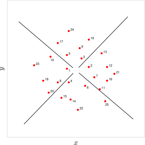
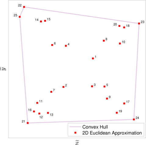
This procedure is illustrated for a set of 25 enumerated points that are separated by impassable line segments, creating a non-Euclidean point cloud as shown in Fig. LABEL:Im1a:_PointCloud. The 2D Euclidean approximate coordinates that define matrix $\widetilde{X}$ are shown in Fig. LABEL:Im1b:_MDSAppx where the pairwise Euclidean distances approximate the pairwise shortest paths of the original non-Euclidean point cloud. Also shown is the convex hull of these 2D points that initiates the subtour of the ACHCI heuristic.

(a)

(b)

Figure 2: ACHCI subtour initiation and complete tour for the non-Euclidean TSP instance with 25 points

The ACHCI algorithm is summarized as:

1. Initiate subtour as the convex hull nodes of $\widetilde{X}$. Next, discard the Euclidean point approximation and use the true non-Euclidean arc costs of the $C$ matrix for the remaining steps of the ACHCI algorithm.

2. Find consecutive nodes $v_{i},v_{j}\in V$ in the subtour and $v_{k}\in V$ not in the subtour, that minimizes non-Euclidean insertion cost ratio $(C_{ik}+C_{kj})/C_{ij}$.

3. Insert $v_{k}$ between $v_{i}$ and $v_{j}$, updating the subtour.

4. Repeat Step 2 and Step 3, to obtain a Hamiltonian cycle.

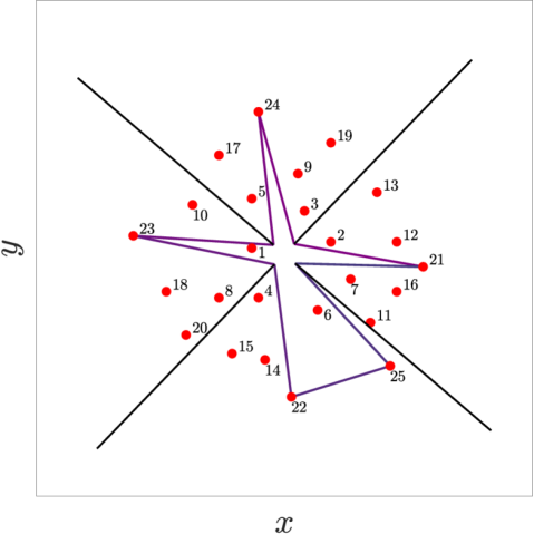
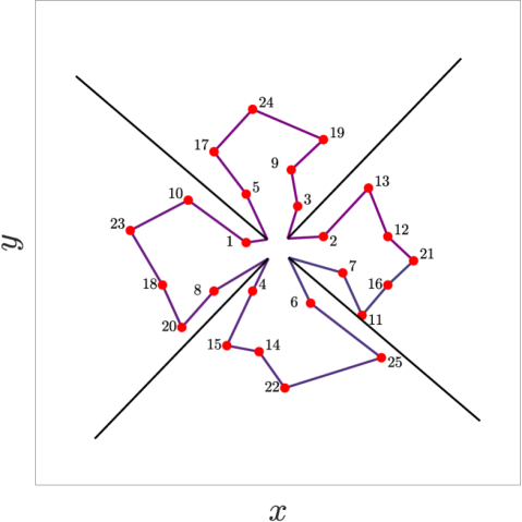
For the example set of 25 non-Euclidean points, the subtour is initiated using the convex hull boundary points of $\widetilde{X}$ as shown in Fig. LABEL:Im1c:_CHullInit, after which the Euclidean coordinate approximation is discarded. The insertion cost ratios of Step 2, 3 and 4 use the true non-Euclidean cost matrix $C$ to obtain the complete tour, as shown in Fig. LABEL:Im1d:_ACHCIsol.

4 Nearest Neighbor Heuristic

The NN heuristic, which is a fast and simple greedy selection rule [35] is chosen as the benchmark algorithm because it is known experimentally to perform reasonably well [36] and is commonly seen in constrained TSP literature [16, 17, 18, 19, 20]. Starting from a predefined or randomly selected initial node, the NN algorithm assigns the unvisited node associated with the lowest cost as the next node, until all nodes are contained in the tour. The NN algorithm is as described below:

1. Initiate the subtour as the starting location

2. Append the subtour with the location with lowest non-Euclidean cost with respect to the location that is at the end of the current subtour

3. Repeat step 2 until all locations have been included

4. Return to the starting location

5 Computational Experiments

To compare the effectiveness of the ACHCI algorithms with the NN algorithm, sufficiently diverse benchmark instances are not readily available for the non-Euclidean TSP. For this reason, the popular TSPLIB benchmark instances [29] are modified in a reproducible manner, to add impassable separators as environmental constraints. The procedure to obtain these non-Euclidean point clouds is as follows:

1. Load a TSPLIB point cloud that has 2D Cartesian coordinates defined for every point. Let $n$ be the number of points.

2. Find the centroid of the point cloud.

3. Sort and assign indices to the points in order of increasing distance from the centroid. Let the indices be $1,2,...,n$ for the sorted points.

4. Draw a line segment from the centroid to the farthest point. Trim its length by 5% from both ends. This line segment functions as an impassable separator $A$.

5. For $k$ equiangular separators, rotate copies of separator $A$ about the centroid by multiples of $2\pi/k$ radians. The TSPLIB point cloud is now modified to a non-Euclidean space by these impassable separators.

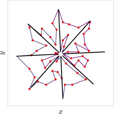
As an example, the ‘eil51’ instance with 8 added separators is shown in Fig. 3 along with the ACHCI tour obtained. Let the resulting non-Euclidean point cloud be represented by the graph $\mathcal{G}:=(V,A)$, with $|V|=n$ points. The $k$ impassable separators of Steps 4 and 5 induce deviations from straight-line paths for a number of points in set $V$. For each pair of points $u,v\in V$, the Euclidean distance is denoted by $\delta(u,v)$ while $\Delta(u,v)$ is the shortest true path length between them, computed using Dijkstra’s shortest path algorithm [37]. The distortion of the Euclidean space caused by these impassable objects is quantified in literature [2, 38] by the deviation factor (DF), where

$$DF={|V|\choose 2}^{-1}\sum_{\begin{subarray}{c}(u,v)\in A\\ u\neq v\end{subarray}}\frac{\Delta(u,v)}{\delta(u,v)}$$ (5)

is the average ratio of true path length to Euclidean path length.

Table 1: Percentage reduction of NN heuristic cost when using ACHCI

TSPLIB instance	Number of Separators
	0	2	4	8	16	32
eil51	15.5	18.9	13.8	-6.7	7.3	4.8
t70	10.1	13.8	13.2	3.1	2.8	-2.8
eil76	6.9	14.0	11.1	7.7	3.3	2.5
erlin52	15.4	17.4	9.9	11.9	11.7	8.2
eil101	16.0	15.3	16.5	8.6	8.3	4.0
rat99	15.7	12.1	13.4	17.6	11.6	1.2
pr76	25.6	20.7	20.1	6.4	6.8	9.1
roC100	12.0	19.6	18.0	22.4	7.3	7.7
roD100	21.8	21.3	8.9	9.4	12.3	3.5
roE100	15.1	13.0	15.4	5.6	4.1	4.4
roA100	14.5	18.0	16.6	11.6	7.5	1.3
roB100	15.9	8.9	10.2	6.2	5.1	3.5
in105	20.5	13.5	14.0	14.8	8.0	1.4
pr107	5.5	13.4	13.9	14.0	13.6	11.9
pr124	9.8	12.6	20.8	7.1	2.1	3.1
roB150	21.5	18.2	13.8	10.2	5.7	-0.6
roA150	12.9	17.9	20.6	13.5	6.4	0.6
pr136	14.9	18.3	15.3	14.4	1.3	-4.7
pr144	5.4	2.1	0.0	2.8	7.7	3.5
pr152	5.1	10.6	19.5	19.9	16.6	8.9
rat195	9.7	11.4	13.8	8.6	6.2	-2.0
bier127	14.7	16.4	19.1	15.7	9.6	14.0
roA200	17.9	16.0	17.6	18.6	12.9	3.3
roB200	14.7	11.6	10.2	16.7	14.5	0.9
rd100	18.1	14.8	9.6	6.9	-1.5	-0.6
gil262	11.6	16.5	10.2	4.3	7.8	-4.8
pr226	12.7	18.5	23.8	8.6	5.6	4.1
a280	17.5	15.4	20.2	15.4	10.3	3.8
ts225	6.8	-0.7	-2.7	4.4	1.0	-6.0
pr264	3.9	3.7	9.1	6.4	7.2	8.6

TSPLIB instance	Number of Separators
	0	2	4	8	16	32
tsp225	14.7	21.4	19.5	16.3	13.9	9.3
pr299	18.0	14.7	8.6	17.1	12.5	1.9
in318	12.5	15.2	11.6	12.2	7.7	2.8
in318	12.5	15.2	11.6	12.2	7.7	2.8
h130	6.7	13.0	13.9	1.1	-0.1	-1.4
u159	19.5	15.7	7.3	9.7	1.5	2.1
h150	8.6	15.7	19.8	11.9	-6.0	-0.7
d198	9.3	4.8	4.2	4.7	12.2	5.6
pr439	14.2	14.7	12.2	10.7	8.0	4.5
rat575	10.1	16.4	13.0	13.5	13.1	4.6
rat783	14.8	16.2	13.1	13.9	15.8	12.1
rd400	14.8	12.6	15.6	10.6	9.6	-4.8
fl417	12.5	16.9	20.4	11.9	8.2	4.6
pcb442	13.6	11.1	13.1	11.7	7.5	1.2
d493	13.3	10.2	18.0	18.1	13.9	17.6
pr1002	16.0	11.0	15.8	14.2	12.4	6.2
u574	13.9	17.9	14.7	14.1	14.2	1.6
p654	19.9	15.4	21.7	12.1	3.4	6.9
d657	13.7	16.8	18.9	24.4	19.8	8.8
u724	11.2	16.3	14.2	16.8	14.2	8.8
u1060	15.3	15.4	18.0	12.3	12.5	5.6
vm1084	12.6	12.7	12.6	16.3	14.0	7.3
nrw1379	11.1	13.3	12.8	17.2	17.5	14.9
pcb1173	14.8	12.1	16.8	12.3	15.2	9.6
d1291	10.2	10.9	16.5	11.9	12.3	12.5
rl1304	11.6	16.3	12.5	12.4	11.4	4.7
rl1323	13.2	13.4	13.3	13.4	5.6	5.1
fl1400	22.6	16.3	14.8	9.0	4.7	7.1
u1432	13.7	11.0	10.1	12.8	12.4	7.1
fl1577	13.2	13.1	9.7	11.3	9.4	13.1

Figure 3: ACHCI tour for the TSPLIB instance ‘eil51’ with 8 separators

(a)

(b)

(c)

Figure 4: Performance analysis of the ACHCI algorithm and Nearest Neighbor for TSP problems without precendence constraints.

To analyze the performance of the ACHCI algorithm, extensive computational experiments were conducted in a Matlab R2023b environment on an AMD Ryzen 5600X CPU clocked at 3.7 GHz. The results of these experiments are summarized in Table 1, where the first column lists the name of each TSPLIB instance, formatted with a prefix followed by a numeric value that indicates the number of points in the respective instance. The experiments are conducted for 60 TSPLIB instances, with the number of points varying from 51 to 1,577. Each TSPLIB instance is modified to generate various deviation factors by following the previously outlined steps to add 0, 2, 4, 8, 16 or 32 impassable separators. For increasing DF caused by the addition of these separators, the remaining columns of Table 1 indicate the observed percentage reductions in NN tour costs, achieved by using the ACHCI heuristic.

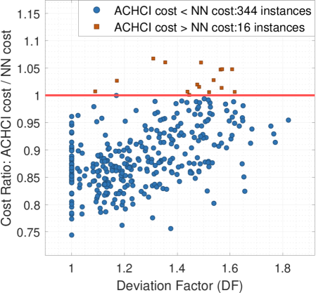
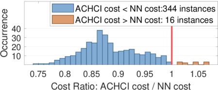
To visualize the effect of DF, the ratio of tour costs obtained using the ACHCI heuristic to that obtained using the NN heuristic is shown in Fig. LABEL:Im_5b:_Performance-NETSP. It is clear that the ACHCI algorithm largely outperforms the NN heuristic regardless of the DF, indicating that the proposed heuristic is well suited to a variety of non-Euclidean point cloud configurations. For the cases with no separators, that is, for DF $=1$, it is seen that the ACHCI cost is always lower than the NN cost. For increasing DF, a diminishing trend is observed in the advantage that the ACHCI algorithm provides, which can be attributed to the increasing degree of approximation caused by the MDS when it projects points to Euclidean 2D space. On average, the ACHCI tour cost is 11% lower than that of the NN heuristic, and the distribution of cost reduction ratios is shown in the histogram of Fig. LABEL:Im_5c:_Res-NETSP.

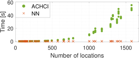
The computation time taken by the two heuristics are shown in Fig. LABEL:time, indicating a worst-case complexity of $O(n^{3})$. This is attributed to the eigenvalue decomposition involved with MDS and the cheapest insertion criteria used when selecting points while building the tour. In comparison, regardless of the number of points, the NN heuristic almost instantaneously provides tours, and in 16 of the studied 334 cases, the NN tour cost is lower than the ACHCI cost. Based on the computational budget, it may therefore be worthwhile to compute both the NN and the ACHCI tour and select the tour with lower cost.

6 Conclusion

The well-known Euclidean CHCI algorithm has been adapted for non-Euclidean instances of the TSP. This is accomplished by first utilizing the MDS algorithm to generate an equivalent set of 2D point coordinates with pairwise distances that best approximate the non-Euclidean cost function. While the convex hull is drawn over these equivalent points to initiate the ACHCI algorithm, the subsequent insertions are based on the true non-Euclidean costs. To study the performance of the algorithm, TSPLIB instances were modified to create non-Euclidean point clouds by adding impassable separators. The ACHCI algorithm produced better tour costs than the Nearest Neighbor algorithm in 96% of the cases studied.

Future work will focus on extending the CHCI algorithm to study its ability to account for other real-world constraints such as precedence constraints relevant to the pickup and delivery problem, the multi-commodity one-to-one pickup-and-delivery traveling salesman problem, and the dial-a-ride problem. The developed heuristics will then be utilized to initialize upper bounds for exact solvers like branch and bound for faster convergence.

References

- [1] J. Saalweachter, Z. Pizlo, Non-euclidean traveling salesman problem, in: Decision modeling and behavior in complex and uncertain environments, Springer, 2008, pp. 339–358.
- [2] B. Boyacı, T. H. Dang, A. N. Letchford, Vehicle routing on road networks: How good is euclidean approximation?, Computers & Operations Research 129 (2021) 105197.
- [3] H. Alkema, M. de Berg, M. Monemizadeh, L. Theocharous, Tsp in a simple polygon, in: 30th Annual European Symposium on Algorithms (ESA 2022), Schloss Dagstuhl-Leibniz-Zentrum für Informatik, 2022.
- [4] M. Goutham, S. Boyle, M. Menon, S. Mohan, S. Garrow, S. Stockar, Optimal path planning through a sequence of waypoints, IEEE Robotics and Automation Letters (2023).
- [5] J. Faigl, M. Kulich, V. Vonásek, L. Přeučil, An application of the self-organizing map in the non-euclidean traveling salesman problem, Neurocomputing 74 (5) (2011) 671–679.
- [6] F. Glover, G. Gutin, A. Yeo, A. Zverovich, Construction heuristics for the asymmetric tsp, European Journal of Operational Research 129 (3) (2001) 555–568.
- [7] J. Jamal, G. Shobaki, V. Papapanagiotou, L. M. Gambardella, R. Montemanni, Solving the sequential ordering problem using branch and bound, in: 2017 IEEE Symposium Series on Computational Intelligence (SSCI), IEEE, 2017, pp. 1–9.
- [8] G. Shobaki, J. Jamal, An exact algorithm for the sequential ordering problem and its application to switching energy minimization in compilers, Computational Optimization and Applications 61 (2) (2015) 343–372.
- [9] Y. Salii, Revisiting dynamic programming for precedence-constrained traveling salesman problem and its time-dependent generalization, European Journal of Operational Research 272 (1) (2019) 32–42.
- [10] Z. Xiang, C. Chu, H. Chen, The study of a dynamic dial-a-ride problem under time-dependent and stochastic environments, European Journal of Operational Research 185 (2) (2008) 534–551.
- [11] K.-I. Wong, A. Han, C. Yuen, On dynamic demand responsive transport services with degree of dynamism, Transportmetrica A: Transport Science 10 (1) (2014) 55–73.
- [12] N. Marković, R. Nair, P. Schonfeld, E. Miller-Hooks, M. Mohebbi, Optimizing dial-a-ride services in maryland: benefits of computerized routing and scheduling, Transportation Research Part C: Emerging Technologies 55 (2015) 156–165.
- [13] K. Braekers, A. Caris, G. K. Janssens, Exact and meta-heuristic approach for a general heterogeneous dial-a-ride problem with multiple depots, Transportation Research Part B: Methodological 67 (2014) 166–186.
- [14] M. A. Masmoudi, M. Hosny, K. Braekers, A. Dammak, Three effective metaheuristics to solve the multi-depot multi-trip heterogeneous dial-a-ride problem, Transportation Research Part E: Logistics and Transportation Review 96 (2016) 60–80.
- [15] É. D. Taillard, A linearithmic heuristic for the travelling salesman problem, European Journal of Operational Research 297 (2) (2022) 442–450.
- [16] A. Grigoryev, O. Tashlykov, Solving a routing optimization of works in radiation fields with using a supercomputer, in: AIP Conference Proceedings, Vol. 2015, AIP Publishing LLC, 2018, p. 020028.
- [17] X. Bai, M. Cao, W. Yan, S. S. Ge, X. Zhang, Efficient heuristic algorithms for single-vehicle task planning with precedence constraints, IEEE Transactions on Cybernetics 51 (12) (2020) 6274–6283.
- [18] T. S. Kumar, M. Cirillo, S. Koenig, On the traveling salesman problem with simple temporal constraints, in: Tenth Symposium of Abstraction, Reformulation, and Approximation, 2013.
- [19] E. Nunes, M. McIntire, M. Gini, Decentralized allocation of tasks with temporal and precedence constraints to a team of robots, in: 2016 IEEE International Conference on Simulation, Modeling, and Programming for Autonomous Robots (SIMPAR), IEEE, 2016, pp. 197–202.
- [20] S. Edelkamp, M. Lahijanian, D. Magazzeni, E. Plaku, Integrating temporal reasoning and sampling-based motion planning for multigoal problems with dynamics and time windows, IEEE Robotics and Automation Letters 3 (4) (2018) 3473–3480.
- [21] L. Ivanova, A. Kurkin, S. Ivanov, Methods for optimizing routes in digital logistics, in: E3S Web of Conferences, Vol. 258, EDP Sciences, 2021, p. 02015.
- [22] A. Warburton, Worst-case analysis of some convex hull heuristics for the euclidean travelling salesman problem, Operations research letters 13 (1) (1993) 37–42.
- [23] V. G. Deineko, R. Van Dal, G. Rote, The convex-hull-and-line traveling salesman problem: A solvable case, Information Processing Letters 51 (3) (1994) 141–148.
- [24] S. Eilon, C. D. T. Watson-Gandy, N. Christofides, R. de Neufville, Distribution management-mathematical modelling and practical analysis, IEEE Transactions on Systems, Man, and Cybernetics (6) (1974) 589–589.
- [25] B. Golden, L. Bodin, T. Doyle, W. Stewart Jr, Approximate traveling salesman algorithms, Operations research 28 (3-part-ii) (1980) 694–711.
- [26] S. Kou, B. Golden, S. Poikonen, Optimal tsp tour length estimation using sammon maps, Optimization Letters (2022) 1–17.
- [27] J. VanDrunen, K. Nam, M. Beers, Z. Pizlo, Traveling salesperson problem with simple obstacles: The role of multidimensional scaling and the role of clustering, Computational Brain & Behavior (2022) 1–13.
- [28] X. Huang, H. Peng, Efficient mobility-on-demand system with ride-sharing, in: 2018 21st International Conference on Intelligent Transportation Systems (ITSC), IEEE, 2018, pp. 3633–3638.
- [29] G. Reinhelt, TSPLIB: a library of sample instances for the tsp (and related problems) from various sources and of various types, URL: http://comopt.ifi.uni-heidelberg.de/software/TSPLIB95/ (2014).
- [30] A. Mead, Review of the development of multidimensional scaling methods, Journal of the Royal Statistical Society: Series D (The Statistician) 41 (1) (1992) 27–39.
- [31] G. A. Seber, Multivariate observations, John Wiley & Sons, 2009.
- [32] W. S. Torgerson, Multidimensional scaling: I. theory and method, Psychometrika 17 (4) (1952) 401–419.
- [33] G. Crippen, Note rapid calculation of coordinates from distance matrices, Journal of Computational Physics 26 (3) (1978) 449–452.
- [34] G. M. Crippen, T. F. Havel, Stable calculation of coordinates from distance information, Acta Crystallographica Section A: Crystal Physics, Diffraction, Theoretical and General Crystallography 34 (2) (1978) 282–284.
- [35] M. F. Dacey, Selection of an initial solution for the traveling-salesman problem, Operations Research 8 (1) (1960) 133–134.
- [36] M. Charikar, R. Motwani, P. Raghavan, C. Silverstein, Constrained tsp and low-power computing, in: Workshop on Algorithms and Data Structures, Springer, 1997, pp. 104–115.
- [37] E. W. Dijkstra, A note on two problems in connexion with graphs, in: Edsger Wybe Dijkstra: His Life, Work, and Legacy, 2022, pp. 287–290.
- [38] J. P. Cole, C. A. King, Quantitative geography: Techniques and theories in geography, Tech. rep. (1968).