Probabilistic Circuits That Know What They Don’t Know

Abstract

Probabilistic circuits (PCs) are models that allow exact and tractable probabilistic inference. In contrast to neural networks, they are often assumed to be well-calibrated and robust to out-of-distribution (OOD) data. In this paper, we show that PCs are in fact not robust to OOD data, i.e., they don’t know what they don’t know. We then show how this challenge can be overcome by model uncertainty quantification. To this end, we propose tractable dropout inference (TDI), an inference procedure to estimate uncertainty by deriving an analytical solution to Monte Carlo dropout (MCD) through variance propagation. Unlike MCD in neural networks, which comes at the cost of multiple network evaluations, TDI provides tractable sampling-free uncertainty estimates in a single forward pass. TDI improves the robustness of PCs to distribution shift and OOD data, demonstrated through a series of experiments evaluating the classification confidence and uncertainty estimates on real-world data.

1 Introduction

The majority of modern machine learning research concentrates on a closed-world setting [Boult et al., 2019]. Here, the value of a model is judged by its performance on a dedicated train-validation-test split from a joint data distribution. Such a focus discounts crucial requirements for real-world inference, where data with a shift in distribution, conceptually novel data, or various combinations of unfiltered corruptions and perturbations are typically encountered [Boult et al., 2019, Hendrycks and Dietterich, 2019]. It is well known that the latter scenarios impose a significant challenge for current practice, attributed to a common culprit referred to as overconfidence [Matan et al., 1990]. Specifically, popular discriminative approaches like SVMs [Scheirer et al., 2013, 2014] and neural networks [Nguyen et al., 2015, Amodei et al., 2016, Guo et al., 2017] chronically assign probabilities close to unity to their predictions, even when a category does not yet exist in the present model.

Figure 1: Conventional PCs are incapable of identifying OOD datasets (solid colors, outlier percentage should be large) while retaining correct predictions for ID data (dashed red, outlier percentage needs to be low to avoid rejection) independently of the decision threshold on the model’s predictive entropy. Whereas their OOD detection precision drops rapidly with increasing threshold, TDI successfully distinguishes ID from OOD data across a wide range.

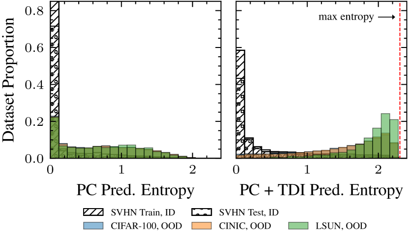
Unfortunately, the above challenge is not limited to discriminative models and has recently resurfaced in the context of generative models. Various works [Nalisnick et al., 2019, Ovadia et al., 2019, Mundt et al., 2022] have empirically demonstrated that different deep models, such as variational auto-encoders [Kingma and Welling, 2014] or normalizing flows [Kobyzev et al., 2020, Papamakarios et al., 2021], have analogous difficulties in separating data from arbitrary distributions from those observed during training. Intuitively speaking, these models “don’t know what they don’t know”. In this paper, we show that a fairly new family of generative models, probabilistic circuits (PCs) [Choi et al., 2020], suffer from the same fate. Until now, these models have been generally assumed to overcome the overconfidence problem faced by their deep neural network counterparts, see e.g. [Peharz et al., 2020a], ascribed primarily to PCs’ ability for tractable and exact inference. This assumption should clearly be challenged, as highlighted by our empirical evidence in the left panel of Fig. 1. Here, we show the percentage of samples recognized as outliers based on the predictive entropy $\sum_{c}p\left(y_{c}|x\right)\log p\left(y_{c}|x\right)$, with labels $y$, classes $c$, and data $x$, obtained by a PC in a classification scenario trained on an in-distribution (ID) dataset and tested on several out-of-distribution (OOD) datasets. When correctly identifying e.g. 95% of SVHN as ID, the PC is only able to detect 24% of the LSUN dataset successfully as OOD.

Inspired by the neural network literature, we consequently posit that PCs’ inability to successfully recognize OOD instances is due to a lack of uncertainty quantification in their original formulation. More specifically, the ability to gauge the uncertainty in the model’s parameters (also called epistemic uncertainty) [Kendall and Gal, 2017, Hüllermeier and Waegeman, 2021] is required to indicate when the output is expected to be volatile and should thus not be trusted. In Bayesian neural networks [MacKay, 1992], such uncertainty is achieved by placing a distribution on the weights and capturing the observed variation given some data. In arbitrary deep networks, the popular Monte Carlo dropout (MCD) [Gal and Ghahramani, 2016] measures uncertainty by conducting stochastic forward passes through a model with dropout [Srivastava et al., 2014], as a practical approximation based on Bernoulli distributions on the parameters.

In our work, we draw inspiration from the MCD approach and build upon its success to quantify the uncertainty in PCs. However, in a crucial difference to neural networks and as the key contribution of our paper, we derive a closed-form solution to MCD leveraging the PC structure’s clear probabilistic semantics. We refer to the derived procedure as tractable dropout inference (TDI), which provides tractable uncertainty quantification in an efficient single forward pass by means of variance propagation. The right panel of Fig. 1 highlights how TDI successfully alleviates the overconfidence challenge of PCs and remarkably improves the OOD detection precision over the entire range of threshold values. Measured over all OOD detection thresholds, TDI improves OOD precision over PCs without TDI by 2.2$\times$ on CIFAR-100 and CINIC, and 2.7$\times$ on LSUN (see Section 4 for details). In summary, our key contributions are:

1. We show that PCs suffer from overconfidence and fall short in distinguishing ID from OOD data.

2. We introduce TDI, a novel inference routine that provides tractable uncertainty estimation. For this purpose, we derive a sampling-free analytical solution to MCD in PCs via variance propagation.

3. We demonstrate TDI’s robustness to distribution shifts and OOD data in three key scenarios with OOD data of different datasets, perturbed, and corrupted instances.

2 Related Work

The primary purpose and goal of our work is to introduce tractable uncertainty quantification to PCs to effectively perform OOD detection, an important aspect that has previously received little to no attention. On a broader scale, the current literature reflects minimal endeavors targeted at enhancing the robustness of PCs. These works undertake the challenge from different perspectives. For instance, to tackle overconfidence on in-domain misclassified samples when data is scarce, Deratani Mauá et al. [2018] introduced costly inference routines based on credal sets that forgo tractable and general inference. Recently, Peddi et al. [2022] presented a likelihood loss to involve artificially perturbed samples during optimization. Although sharing the common aspect of challenging the robustness of PCs, none of these works has provided an efficient tractable uncertainty quantification method to make arbitrary PCs more robust to different OOD data without altering the model’s parameters or compromising inference tractability. Thus, our most closely related works reside in the respective area of uncertainty quantification, in particular, the imminently related approximations made in neural network counterparts [Blundell et al., 2015, Gal and Ghahramani, 2016, Kendall and Gal, 2017]. Gauging such model uncertainty in turn provides substantial value in various tasks, including OOD detection, robustness to corrupt and perturbed data, and several downstream applications. We provide a brief overview of the latter for the purpose of completeness, before concentrating on the essence of our paper in terms of immediately related methodology to estimate model uncertainty.

OOD Detection and Use of Uncertainty: Uncertainty quantification based on Bayesian methods provides a theoretical foundation to assess when a model lacks confidence in its parameters and predictions. Alternatively, several other directions have been proposed to deal with OOD inputs in the inference phase. Notably, several works across the decades have proposed to include various forms of reject options in classification. These methods are often criticized for their lack of theoretical grounding, leading to a separate thread advocating for the challenge to be addressed through open set recognition. We point to the recent review of Boult et al. [2019] for an overview of techniques. In a similar spirit, assessment of uncertainty has been shown to be foundational in the application to e.g. active learning [Gal et al., 2017] or continual learning [Ebrahimi et al., 2020]. We emphasize that these techniques and applications are complementary to our work and are yet to be explored in PCs. Similarly to prior neural network-based efforts of Ovadia et al. [2019] and Nalisnick et al. [2019], we first show that PCs are incapable of inherent OOD detection, before leaning on uncertainty to overcome the challenge with our TDI.

Uncertainty Quantification: In a simplified picture, methods to estimate uncertainty could be attributed to two main categories: methods falling into a Bayesian framework and alternative non-Bayesian ones. As the categorization suggests, the latter do not ground their principle in Bayesian statistics and provide quantification in different forms, such as the size of a prediction interval or a score  [Osband et al., 2021, Yu et al., 2022]. In contrast, Bayesian methods rely on a solid theoretical ground that allows for a clear interpretation. When applied to computation graphs like neural networks and PCs, the key concept is to have a probability distribution over the parameters, in this context, the weights of the graph. More formally, the model parameterization is framed as picking the parameters $\bm{\theta}$ (subject to optimization) from a prior probability distribution $p(\bm{\theta})$. We are then interested in the parameter configuration that most likely represents the data $\mathcal{D}$, i.e., $\operatorname*{arg\,max}_{\bm{\theta}}p(\bm{\theta}|\mathcal{D})$. To account for model uncertainty, it would be necessary to integrate over the parameters, which is intractable for many models.

A considerable number of works have pursued this direction for deep neural architectures. Bayesian neural networks [MacKay, 1992, Neal, 2012] have initially paved the way to model uncertainty, but given the immense computational cost, alternatives focus on several cheap approximations. Popular ways are to back-propagate uncertainty through the gradients [Blundell et al., 2015, Hernández-Lobato and Adams, 2015, Mishkin et al., 2018, Maddox et al., 2019], make use of variational inference [Graves, 2011, Louizos and Welling, 2016] or draw connections to Gaussian Processes  [Gal and Ghahramani, 2016, Khan et al., 2019]. A related approximate approach is based on ensembles, where the underlying idea is to relate the model uncertainty with the statistics computed over the various ensemble components. To obtain uncertainty estimates, most of these approaches need to train multiple ensemble components [Hansen and Salamon, 1990, Lakshminarayanan et al., 2017] or larger overparameterized singletons and treat them as an ensemble of subnetworks [Antorán et al., 2020, Daxberger et al., 2021]. Among the Bayesian methods for learning a PC on propositional knowledge bases, Cerutti et al. [2022] deal with uncertainty estimation for conditional boolean queries by attaching a second circuit to the PC.

Monte Carlo Dropout: The natural question for Bayesian methods is how to sample the parameters $\bm{\theta}$ from the posterior $p\left(\bm{\theta}\,|\,\mathcal{D}\right)$, taking the high-dimensional and highly non-convex nature of the probability distribution for complex networks into account, which leads to intractable standard sampling methods [Izmailov et al., 2021]. Gal and Ghahramani [2016] have reframed dropout [Srivastava et al., 2014] as a Bayesian approximation to assess model uncertainty. Originally, dropout is a method proposed to avoid overfitting and improve generalization by including a stochastic chance $p$ of removing a connection between units of an adjacent layer. Gal and Ghahramani [2016]’s key realization is that dropout allows to cheaply sample from the posterior under the assumption of a Bernoulli distribution on the weights. In essence, MCD approximates the integration over the parameters with a summation over a finite set of $n$ drawn sets of parameters $\bm{\theta}_{i}\sim p\left(\bm{\theta}\,|\,\mathcal{D}\right)$. By using the set of $n$ predicted values, the first and the second raw moments can be computed. The former is then used as the prediction and the latter as an estimate of model uncertainty.

The essential advantage of MCD is its simple applicability, which has led to a wide range of immediate applications [Kendall and Gal, 2017, Gal et al., 2017, Kendall et al., 2017, Miller et al., 2018]. In our work, we draw inspiration from MCD and its vast impact. However, instead of approximating the uncertainty with a Monte Carlo simulation in PCs, we perform variance propagation from the leaf to the root nodes with a single pass, with which we derive a sampling-free, closed-form solution to model uncertainty.

3 Tractable Dropout Inference

In this section, we first introduce preliminaries with respect to PCs, before continuing to delve into a step-by-step derivation of how to obtain sampling-free uncertainties with TDI.

3.1 Preface: Probabilistic Circuits

In this work, we refer to a relevant class of PCs, i.e., sum-product networks (SPNs) [Poon and Domingos, 2011]. In the family of tractable probabilistic models, SPNs stand out for their inference capabilities and great representational power [Delalleau and Bengio, 2011]. They hold important structural properties such as smoothness and decomposability that enable the efficient encoding of a valid probability distribution. In the following, we first formally introduce SPNs and their important properties.

(a) Probabilistic inference

(b) Monte Carlo dropout inference

(c) Tractable dropout inference

Figure 2: Forward pass illustration of a PC (2(a)), a PC with MCD sampling (2(b)), and a PC with TDI based on variance propagation through the graph (2(c)). Whereas a single MCD forward pass only simulates one instantiation of a possible subgraph, the PC with TDI directly propagates the variances through the graph in a single pass (expectations and covariances are left out for visual clarity in the illustration, see Section 3.2 for full equations).

Definition: An SPN $\mathcal{S}$ is a computational graph defined by a rooted directed acyclic graph (DAG), encoding a probability distribution $p_{\mathbf{X}}$ over a set of random variables (RVs) $\mathbf{X}=\{X_{1},\ldots,X_{n}\}$, where inner nodes are either sum nodes $\mathsf{S}$ or product nodes $\mathsf{P}$ over their children, and leaves $\mathsf{L}$ are valid probability distributions defined on a subset of the RVs $\mathbf{Z}\subseteq\mathbf{X}$. Each node $\mathsf{N}\in\mathcal{S}$ has a scope, $\mathbf{sc}\left(\mathsf{N}\right)\subseteq\mathbf{X}$, defined as the set of RVs appearing in its descendant leaves. Each edge $(\mathsf{S}_{i}\rightarrow\mathsf{N}_{j})$ connecting a sum node $\mathsf{S}_{i}$ to one of its children $\mathsf{N}_{j}\in\mathbf{ch}\left(\mathsf{S}_{i}\right)$ has a non-negative weight $w_{ij}$, with $\sum_{j}w_{ij}=1$. Sum nodes represent mixtures over the probability distributions encoded by their children, while product nodes represent factorizations over contextually independent distributions. In summary, an SPN can be viewed as a deep hierarchical mixture model of different factorizations. An illustration of this kind of PC is shown in Fig. 2(a).

To encode a valid probability distribution, an SPN has to fulfill two structural requirements [Poon and Domingos, 2011]. One is decomposability, i.e., the scopes of the children of each product node need to be disjoint, which allows distributing the NP-hard computation of integrals (e.g. the partition function), to leaves where we require this computation to be tractable. This condition can be fulfilled, either by an explicit form, e.g., from an exponential family distribution, or by the architectural design of the leaf density estimators. The second requirement is smoothness, constraining the scopes of the children of each sum node to be identical (this is also referred to as completeness). This constraint is important to encode a valid distribution that does not over- or underestimate some RVs states. In a valid SPN, the probability assigned to a given state $\mathbf{x}$ of the RVs $\mathbf{X}$ is given by the root node and will be denoted as $\mathcal{S}(\mathbf{x})=p_{\mathbf{X}}(\mathbf{X}=\mathbf{x})$.

Tractable Inference: Given an SPN $\mathcal{S}$, $\mathcal{S}\!\left(\mathbf{x}\right)$ is computed by evaluating the network bottom-up. When evaluating a leaf node $\mathsf{L}_{i}$ with scope $X_{j}$, $\mathsf{L}_{i}\!\left(x_{j}\right)$ corresponds to the probability of the state $x_{j}$. The value of a product node $\mathsf{P}_{i}$ corresponds to the product of its children’s values: $\mathsf{P}_{i}\!\left(\mathbf{x}_{|\mathbf{sc}\left(\mathsf{P}_{i}\right)}\right)=\prod_{\mathsf{N}_{j}\in\mathbf{ch}\left(\mathsf{P}_{i}\right)}\mathsf{N}_{j}(\mathbf{x}_{|\mathbf{sc}\left(\mathsf{N}_{j}\right)})$. The value of a sum node $\mathsf{S}_{i}$ is computed as the weighted sum of its children’s values: $\mathsf{S}_{i}\left(\mathbf{x}_{|\mathbf{sc}\left(\mathsf{S}_{i}\right)}\right)=\sum_{\mathsf{N}_{j}\in\mathbf{ch}\left(\mathsf{S}_{i}\right)}w_{ij}\mathsf{N}_{j}(\mathbf{x}_{|\mathbf{sc}\left(\mathsf{N}_{j}\right)})$. All the exact marginal and conditional probabilities, also with different amount of evidence, the exact partition function, and even approximate most probable explanation and maximum a posteriori states can be computed in time and space linear in the network’s size, i.e. number of edges [Poon and Domingos, 2011, Peharz et al., 2015].

Being part of the PC family, SPNs share the basic building blocks and procedures when performing inference with other classes of PCs. Thus, the contributions that we introduce in this paper can also be easily applied to other models of the PC family [Choi et al., 2020]. We further note that because TDI is presently framed as an inference routine, training follows conventional algorithms. Whereas the inclusion of uncertainties to guide training itself is certainly intriguing, we defer this prospect to future work and concentrate on the means to quantify uncertainty to overcome overconfidence and detect OOD data.

3.2 Deriving TDI

One of the crucial aspects in which PCs stand out compared to neural networks is that they have clear probabilistic semantics. Leaf nodes are normalized tractable distributions and sum nodes represent weighted mixtures over different factorizations, encoded by the product nodes, on the same scope. When dropout is applied to PCs, it thus entails an easier interpretation. At first look, similar to the case for neural networks, MCD at sum nodes would perform a sort of model averaging between a randomly selected set of models (sub-graphs). Naively, we could follow the same procedure as proposed in Gal and Ghahramani [2016] and conduct stochastic forward passes with a more intuitive interpretation on mixtures over different factorizations (compared to a black-box neural network); see Fig. 2(b) for an illustration. The variance of the different models is then interpreted as the uncertainty w.r.t. a specific input. However, we will now show that it is also possible to derive TDI as a tractable uncertainty estimate in a single forward pass in PCs. With our closed-form derivations, we thus provide an analytical solution to this measure of uncertainty.

Core Idea – Sampling-free Uncertainty: The general idea is to derive closed-form expressions of the expectation, variance, and covariance for sum and product nodes as a function of their children. The model uncertainty at the root nodes is then recursively computed by performing variance propagation from the leaf nodes to the root nodes in a single bottom-up pass through the graph structure (see Fig. 2(c)). This procedure results in uncertainty estimates without sampling from the graph multiple times, as is required by MCD.

In TDI we start by viewing sum nodes as linear combinations of RVs over their Bernoulli dropout RVs and their children:

$$\mathsf{S}=\sum_{i}\delta_{i}w_{i}\mathsf{P}_{i}\,,$$ (1)

where $\delta_{i}\sim\text{Bern}\!\left(q\right)$ and $p=1-q$ corresponds to the dropout probability.

We will now provide the expectation, variance, and covariance closed-form solutions for sum, product, and leaf nodes. Here, we present the most relevant derivations for these quantities. For full derivations and theoretical details, we refer to Appendix A.

3.2.1 Expectation: The Point Estimate

Using the linearity of the expectation, we push the expectation into the sum and make use of the independence between the child nodes $\mathsf{N}_{i}$ and the Bernoulli RVs $\delta_{i}$ to extract $\mathbb{E}[\delta_{i}]=q$:

$$\mathbb{E}\!\left[\mathsf{S}\right]=q\sum_{i}w_{i}\mathbb{E}\!\left[\mathsf{N}_{i}\right]\,.$$ (2)

The decomposability of product nodes ensures the independence of their children w.r.t. each other, which leads to the product node expectation simply becoming the product over the expectations of its children, i.e.,

$$\mathbb{E}\!\left[\mathsf{P}\right]=\prod_{i}\mathbb{E}\!\left[\mathsf{N}_{i}\right]\,.$$ (3)

3.2.2 Variance: The Uncertainty Proxy

Similar to the original work in neural networks of Gal and Ghahramani [2016], we will use the variance as the proxy for the uncertainty. The sum node variance decomposes into a sum of two terms. The first term is based on the variances and expectations of its children and the second term accounts for the covariance between the combinations of all children, i.e.,

$$\text{Var}\!\left[\mathsf{S}\right] = q\sum_{i}w_{i}^{2}\left(\text{Var}\!\left[\mathsf{N}_{i}\right]+p\mathbb{E}\!\left[\mathsf{N}_{i}\right]^{2}\right)$$

$$+q^{2}\sum_{i\neq j}w_{i}w_{j}\text{Cov}\!\left[\mathsf{N}_{i},\mathsf{N}_{j}\right]\,.$$ (4)

Analogously, the product node variance decomposes into two product terms. By applying the product of independent variables rule, we obtain:

$$\text{Var}\!\left[\mathsf{P}\right] =\prod_{i}\left(\text{Var}\!\left[\mathsf{N}_{i}\right]+\mathbb{E}\!\left[\mathsf{N}_{i}\right]^{2}\right)-\prod_{i}\mathbb{E}\!\left[\mathsf{N}_{i}\right]^{2}\,.$$ (5)

3.2.3 Covariance: The Evil

The covariance between two sum nodes, $\mathsf{S}^{A}$ and $\mathsf{S}^{B}$, neatly decomposes into a weighted sum of all covariance combinations of the sum node children:

$$\text{Cov}\!\left[\mathsf{S}^{A},\mathsf{S}^{B}\right]=q^{2}\sum_{i}w_{i}^{A}\sum_{j}w_{j}^{B}\text{Cov}\!\left[\mathsf{N}_{i}^{A},\mathsf{N}_{j}^{B}\right]\,.$$ (6)

For an arbitrary graph, we are unable to provide a closed-form solution of the covariance between two product nodes due to the first expectation in the product node covariance:

$$\text{Cov}\!\left[\mathsf{P}^{A},\mathsf{P}^{B}\right] = \mathbb{E}\!\left[\prod_{i}\mathsf{N}_{i}^{A}\prod_{j}\mathsf{N}_{j}^{B}\right]$$

$$-\prod_{i}\mathbb{E}\!\left[\mathsf{N}_{i}^{A}\right]\prod_{j}\mathbb{E}\!\left[\mathsf{N}_{j}^{B}\right]\,,$$ (7)

which cannot be simplified without any structural knowledge about independencies between the children of $\mathsf{N}^{A}$ and $\mathsf{N}^{B}$, as they may share a common subset of nodes, deeper down in the PC structure. Fortunately, we explore three possible solutions to solve Eq. 7 in the following, of which variants b) and c) are always applicable.

a) Structural Knowledge: To simplify Eq. 7 we can easily exploit structural knowledge of the DAG. The simplest solution is a structure in which we know that two product nodes $\mathsf{P}^{A}$ and $\mathsf{P}^{B}$ are not common ancestors of any node, resulting in the independence $\mathsf{P}^{A}\perp\!\!\!\!\perp\mathsf{P}^{B}$ and thus $\text{Cov}[\mathsf{P}^{A},\mathsf{P}^{B}]=0$. This constraint is always given in tree-structured PCs. Because simple in practice, tree structures are generated by the most common structure learner for SPNs such as LearnSPN [Gens and Domingos, 2013], ID-SPN [Rooshenas and Lowd, 2014], and SVD-SPN [Adel et al., 2015].

For binary tree random and tensorized (RAT) structures [Peharz et al., 2020b], Eq. 7 can be simplified to

$$\text{Cov}\!\left[\mathsf{P}_{l,r},\mathsf{P}_{l^{\prime},r^{\prime}}\right]= \text{Cov}\!\left[\mathsf{S}^{L}_{l},\mathsf{S}^{L}_{l^{\prime}}\right]\mathbb{E}\!\left[\mathsf{S}^{R}_{r}\right]\mathbb{E}\!\left[\mathsf{S}^{R}_{r^{\prime}}\right]$$

$$+\, \text{Cov}\!\left[\mathsf{S}^{R}_{r},\mathsf{S}^{R}_{r^{\prime}}\right]\mathbb{E}\!\left[\mathsf{S}^{L}_{l}\right]\mathbb{E}\!\left[\mathsf{S}^{L}_{l^{\prime}}\right]$$

$$+\, \text{Cov}\!\left[\mathsf{S}^{L}_{l},\mathsf{S}^{L}_{l^{\prime}}\right]\text{Cov}\!\left[\mathsf{S}^{R}_{r},\mathsf{S}^{R}_{r^{\prime}}\right]\,.$$ (8)

The covariance of two product nodes now only depends on the covariance of the input sum nodes of the same graph partition ($L$ or $R$) for which we can plug in Eq. 6.

b) It’s Somewhere in Here – Covariance Bounds: Whereas knowledge about the specific PC structure can facilitate the covariance computation, when not available, we can alternatively obtain a lower and upper bound of the covariance, making use of the Cauchy-Schwarz inequality:

$$\text{Cov}\!\left[\mathsf{N}_{i},\mathsf{N}_{j}\right]^{2} \leq\text{Var}\!\left[\mathsf{N}_{i}\right]\text{Var}\!\left[\mathsf{N}_{j}\right]$$ (9)

$$\Leftrightarrow\quad \text{Cov}\!\left[\mathsf{N}_{i},\mathsf{N}_{j}\right] \in\left[-\sqrt{\text{Var}\!\left[\mathsf{N}_{i}\right]\text{Var}\!\left[\mathsf{N}_{j}\right]},\right.$$

$$\left.+\sqrt{\text{Var}\!\left[\mathsf{N}_{i}\right]\text{Var}\!\left[\mathsf{N}_{j}\right]}\right]\quad.$$ (10)

c) The Copy-paste Solution: A third alternative to using structural knowledge or giving covariance bounds is via a “copy-paste” augmentation of the DAG, that enforces the covariance between two nodes, $\mathsf{N}_{A}$ and $\mathsf{N}_{B}$, to be zero by treating their common child as two separate nodes. That is, for each node $\mathsf{N}_{C}$ where a $\text{Path}_{A}:=\mathsf{N}_{A}\rightarrow\mathsf{N}_{C}$ and a second $\text{Path}_{B}:=\mathsf{N}_{B}\rightarrow\mathsf{N}_{C}$ exists, we can “copy” $\mathsf{N}_{C}$ to obtain an equivalent node $\mathsf{N}_{C^{\prime}}$ and replace the original $\mathsf{N}_{C}$ in $\text{Path}_{B}$ with the copy $\mathsf{N}_{C^{\prime}}$. With this simple procedure, we can enforce a tree structure on the PC, resulting in the covariance between two children of a node $\mathsf{N}$ to be zero. In practice, we do not need to modify the DAG. Instead, we can simply ignore the covariance terms and thereby obtain this DAG transformation during the TDI procedure implicitly.

3.2.4 Leaf Nodes

As leaf nodes are free of any dropout Bernoulli variables, their expectation, variance, and covariance degrade to the leaf node value and zero respectively, i.e.,

$$\mathbb{E}\!\left[\mathsf{L}\right]=\mathsf{L},\quad\text{Var}\!\left[\mathsf{L}\right]=0,\quad\text{Cov}\!\left[\mathsf{L}_{i},\mathsf{L}_{j}\right]=0\,.$$ (11)

While the above is a valid choice, this framework further allows including prior knowledge about aleatoric and epistemic uncertainty, by setting $\text{Var}[\mathsf{L}]>0$ and $\text{Cov}[\mathsf{L}_{i},\mathsf{L}_{j}]\neq 0$. This additionally highlights the advantage over the MCD procedure, where the inclusion of prior knowledge is not possible.

3.2.5 Classification Uncertainty

For classification in PCs, we can express the class conditionals $p\left(\mathbf{x}\,|\,y_{i}\right)=\mathsf{S}_{i}$ as root nodes with class priors $p\left(y_{i}\right)=c_{i}$ and obtain the posterior via Bayes’ rule, i.e.,

$$p\left(y_{i}\,|\,\mathbf{x}\right)=\frac{p\left(\mathbf{x}\,|\,y_{i}\right)p\left(y_{i}\right)}{\sum_{j}p\left(\mathbf{x}\,|\,y_{j}\right)p\left(y_{j}\right)}=\frac{\mathsf{S}_{i}c_{i}}{\sum_{j}\mathsf{S}_{j}c_{j}}\,.$$ (12)

In our case, the expectation and variance of the posterior are that of a random variable ratio, $\mathbb{E}\!\left[\frac{A}{B}\right]$ and $\text{Var}\!\left[\frac{A}{B}\right]$, with $A=\mathsf{S}_{i}c_{i}$ and $B=\sum_{j}\mathsf{S}_{j}c_{j}$. This ratio is generally not well-defined, but can be approximated with a second-order Taylor approximation [Seltman, 2018]:

$$\mathbb{E}\!\left[\frac{A}{B}\right] \approx\frac{\mathbb{E}\!\left[A\right]}{\mathbb{E}\!\left[B\right]}-\frac{\text{Cov}\!\left[A,B\right]}{\left(\mathbb{E}\!\left[B\right]\right)^{2}}+\frac{\text{Var}\!\left[B\right]\mathbb{E}\!\left[A\right]}{\left(\mathbb{E}\!\left[B\right]\right)^{3}}$$ (13)

$$\text{Var}\!\left[\frac{A}{B}\right] \approx\frac{\mathbb{E}\!\left[A\right]^{2}}{\mathbb{E}\!\left[B\right]^{2}}\left[\frac{\text{Var}\!\left[A\right]}{\mathbb{E}\!\left[A\right]^{2}}-2\frac{\text{Cov}\!\left[A,B\right]}{\mathbb{E}\!\left[A\right]\mathbb{E}\!\left[B\right]}+\frac{\text{Var}\!\left[B\right]}{\mathbb{E}\!\left[B\right]^{2}}\right].$$ (14)

We will now resolve every component of Eqs. 13 and 14. The expectations are straightforward:

$$\mathbb{E}\!\left[A\right] =\mathbb{E}\!\left[\mathsf{S}_{i}c_{i}\right]=\mathbb{E}\!\left[\mathsf{S}_{i}\right]c_{i}$$ (15)

$$\mathbb{E}\!\left[B\right] =\mathbb{E}\!\left[\sum_{j}\mathsf{S}_{j}c_{j}\right]=\sum_{j}\mathbb{E}\!\left[\mathsf{S}_{j}\right]c_{j}\,.$$ (16)

For the variances we obtain:

$$\text{Var}\!\left[A\right] =\text{Var}\!\left[\mathsf{S}_{i}\right]c_{i}^{2}$$ (17)

$$\text{Var}\!\left[B\right] =\sum_{j}\text{Var}\!\left[\mathsf{S}_{j}\right]c_{j}^{2}+\sum_{j_{1}\neq j_{2}}\text{Cov}\!\left[\mathsf{S}_{j_{1}},\mathsf{S}_{j_{2}}\right]c_{j_{1}}c_{j_{2}}\,.$$ (18)

Following Eq. 6, the covariance term between a root node and the sum of all root nodes can be decomposed as follows:

$$\text{Cov}\!\left[A,B\right] =c_{i}\sum_{j}c_{j}\text{Cov}\!\left[\mathsf{S}_{i},\mathsf{S}_{j}\right]\quad,$$ (19)

which in turn can be resolved with one of the methods provided in Section 3.2.3.

While Eqs. 13 and 14 are seemingly simple, their particular formulation implies statistical independence between $A$ and $B$. Since $B$ is a sum over all $A$, this independence naturally does not hold. Therefore, the solution given here is only an approximation of the true second-order Taylor approximation. In Appendix A.2.7 we extend the formulation of Seltman [2018] and take into account the dependencies between root nodes $\mathsf{S}_{i}$ and their sum $\sum_{i}\mathsf{S}_{i}$.

3.2.6 Tractability

We re-emphasize that PCs are tractable probabilistic models where, in general, inference is at most polynomial in the network size. Specifically, in the PC family, SPNs perform a wide range of queries in linear time in the network size.

Thanks to the compact representation of PCs, all formulations derived for TDI in Sections 3.2.1, 3.2.2, 3.2.3, 3.2.4 and 3.2.5 have polynomial space and time complexity, specifically, at most quadratic. In fact, the expectation of a single sum node, given by Eq. 2, adds a negligible single floating point multiplication (by $q$) as we can reuse the sum node output. The expectation of a single product, in Eq. 3, does not require any additional operations. For the computation of variance and covariance, the cost depends on the actual PC structure. In sparse structures such as trees, the cost is linear with respect to the number of input nodes, as the covariance term becomes zero. However, for cases where all child input covariance combinations need to be computed, as in Eq. 5, the cost can be locally quadratic with respect to the number of sum node inputs (see Sections 3.2.2 and 6). Applying solution c) of Section 3.2.3, i.e., the implicit “copy-paste” augmentation of the DAG, reduces the cost of Eq. 5 to be linear instead of quadratic. This renders a full bottom-up pass tractable, which can be performed in parallel with the standard bottom-up probabilistic inference procedure. We provide pseudocode for the bottom-up TDI in Appendix B.

4 Experimental Evaluation

To demonstrate that PCs generally suffer from overconfidence under various forms of distribution shift, and to show the benefits of TDI in these circumstances, we investigate the following three common experimental scenarios:

1. OOD datasets: Following popular practice to assess whether a model can successfully distinguish known data from unknown OOD instances [Bradshaw et al., 2017, Nalisnick et al., 2019], we train the circuits on SVHN [Netzer et al., 2011] and then additionally test on several popular color image datasets: CIFAR-100 [Krizhevsky, 2009], CINIC [Darlow et al., 2018], and LSUN [Yu et al., 2015].

2. Perturbations: Inspired by recent works that investigate predictions in the context of increasingly perturbed data instances [Ovadia et al., 2019, Antorán et al., 2020, Daxberger et al., 2021], we evaluate our models when rotating MNIST [LeCun et al., 1998] digits are introduced for inference.

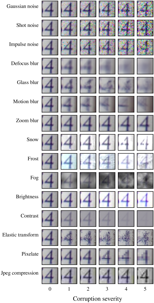
3. Corrupted inputs: In the spirit of recent works that demonstrate standard neural networks’ inability to effectively handle naturally corrupted data [Hendrycks and Dietterich, 2019, Michaelis et al., 2019], we include a set of 15 different non-trivial corruptions to the SVHN dataset for inference with PCs and PCs + TDI. Each of these corruptions features five different levels of severity.

Experimental Setup.

For our experiments, we implemented TDI based on RAT-SPNs in PyTorch and SPFlow [Molina et al., 2019]. We use $S=20,I=20,D=5,R=5$ for the RAT-SPN structure and train our models for 200 epochs with a mini-batch size of 200, a learning rate of 1e-3 with the Adam [Kingma and Ba, 2015] optimizer, and a PC + TDI dropout value of 0.2 for MNIST and 0.1 for SVHN. A detailed description is provided in Appendix C and our code is available at https://github.com/ml-research/tractable-dropout-inference.

4.1 PCs with TDI Detect OOD Data

Following our outlined first scenario, we first train on the SVHN dataset. We then evaluate the predictive entropy obtained on samples of the unseen test set and on instances that come from entirely different distributions of other datasets, e.g. house numbers vs. different scene images or object categories like cars and sofas. To successfully avoid mispredictions on an unrelated unknown dataset, the entropy of our model’s predictions should be higher compared to the one obtained for ID samples. Although predictive entropy might not be the optimal choice for uncertainty quantification [Hüllermeier and Waegeman, 2021], we leave the exploration of better measures, in particular for OOD detection, to future work and remark that our main focus is on assessing whether the epistemic uncertainty estimate obtained with TDI is meaningful or not.

Table 1: PC + TDI (in bold) improves area under curve scores for Fig. 1 over PCs when measuring the OOD precision over all thresholds by more than 2$\times$ on every OOD dataset. TDI is competitive with MCD while being more efficient as it does not require the cost of performing multiple (here 100) stochastic forward passes.

AUC ($\uparrow$)	CIFAR	CINIC	LSUN
PC	29.3	29.9	30.3
PC + TDI	64.6	66.1	81.8
PC + MCD	68.5	70.0	84.9
MLP	56.0	58.1	55.9
MLP + MCD	80.8	95.9	80.5
LeNet	17.1	15.6	2.6
LeNet + MCD	43.4	92.9	29.5

Figure 3: Difference between ID and OOD detection precision of PCs (dashed) and PCs + TDI (solid) for all OOD detection threshold of Fig. 1. PCs with TDI both outperform PCs in absolute terms and allow the model to adequately balance ID versus OOD data. On the contrary, conventional PCs without TDI generally perform poorly and have their best point at an unintuitively low threshold.

Our introductory Fig. 1 has already shown that conventional PCs are bad at properly detecting OOD data while keeping a high precision on ID data, whereas PCs with TDI overcome this challenge. To also quantify the improvement introduced by TDI over all thresholds, we now show the area under the curve scores for Fig. 1 in Table 1, demonstrating that TDI improves all scenarios by more than two times. For a comprehensive overview and as a point of reference, we also present results illustrating that MCD attains analogous improvements on both PCs and neural networks such as a Multilayer Perceptron (MLP) and an inherently overconfident LeNet. However, while MCD requires several stochastic forward passes (100 in this case), by exploiting PCs semantics, TDI achieves similar performance with only a single forward pass.

In addition, we further highlight the precise tradeoff between the ID and OOD precision over all OOD decision thresholds in Fig. 3. In other words, we quantify the precision with which a selected threshold on entropy correctly leads to rejection of unknown OOD data, while at the same time not rejecting ID data in order to classify it correctly. Intuitively, the threshold should balance the latter two, as a very low threshold should simply reject all data, whereas a very high threshold would incorrectly accept any inputs. As visible, this is not the case for PCs, that have their largest margin between ID and OOD error at a very low OOD decision threshold, leading to a high ID error, e.g. 28.7% ID error and 21.8% LSUN OOD error at a threshold of 0.05 (cf. Fig. 1). On the contrary, TDI balances this shortcoming and allows for much higher OOD decision thresholds while keeping a lower ID error, e.g. 13.2% ID error and 10.2% LSUN OOD error at a reasonable mid-way threshold of 0.6 (cf. Fig. 1). A complementary view with predictive entropy and uncertainty in terms of the standard deviation as the square root of Eq. 14 is provided in Appendix D.

4.2 PCs with TDI are More Uncertain on Perturbed Samples

Figure 4: Top panel: predictive entropy (left y-axis, solid) and accuracy (right y-axis, dashed) of a PC (blue circles) and PC + TDI (orange triangles) on a gradual distribution shift of increasing MNIST digit rotations from 0^∘ to 90^∘ (x-axis). TDI already captures the distribution shift at lower degrees of rotation and assigns a much larger predictive entropy to greater rotations than PCs, while retaining predictive accuracy. Bottom panel: complementary view of predictive uncertainty (standard deviation in Eq. 14) in PC + TDI.

Figure 5: Predictive entropy (left y-axis) and accuracy (right y-axis) of a PC (blue circles) and PC + TDI (orange triangles) for increasingly corrupted SVHN data at five severity levels; here, altering brightness, introducing elastic transformation, simulating frost, and adding Gaussian noise. PCs with TDI detect the distribution shift by assigning higher predictive entropy with increasing severity, while at the same time being more robust in predictive accuracy against the corruption.

In addition to the abrupt distribution shift of the prior section, we now inspect the behavior of PCs and PCs + TDI on a more gradual scale in the second scenario. Here, we train on the original MNIST training set. At inference time, we evaluate the models’ predictive entropy on rotated versions of the MNIST test set from 0^∘ to 90^∘ in steps of 5^∘, to simulate a gradual increase in data perturbation. Once more, with the aim of an effective measure for the distribution shift, the model should assign higher predictive entropy and uncertainty with increasing data perturbation. We visualize this experiment in Fig. 4, demonstrating in the top panel, that PCs with TDI (orange triangle) measure the data perturbation already at lower degrees of rotation and assigns a higher entropy to larger rotations than PCs (blue, circles). At the same time, TDI retains the same predictive accuracy. In the bottom panel of Fig. 4, we additionally highlight the measure of uncertainty as the standard deviation of Eq. 14, again confirming the expected increase of uncertainty with increasing data perturbation from an auxiliary viewpoint.

4.3 PCs with TDI are More Robust to Data Corruptions

As outlined in our third scenario, we investigate the case of natural and synthetic data corruptions. We train on the SVHN training set and then evaluate the models on corrupted versions of the SVHN test set, with 15 different corruptions at five increasing levels of severity. Similar to the prior two scenarios, a successful detection entails that the models should be able to attribute a progressive increase in predictive entropy with increasing corruption severity. In Fig. 5 we highlight the model’s behavior on four such corruption types: brightness, elastic transformation, simulated frost, and Gaussian noise (see Appendix E for analogous evidence for all 15 corruption types). Matching the behavior of the perturbation scenario, in all shown corruption settings, a PC with TDI can associate an increase in corruption severity with higher predictive entropy. On top of that, TDI stays more robust at all severity levels of corruption than the PC by retaining higher predictive accuracy in the case of elastic transformation and Gaussian noise corruptions. This third scenario thus further verifies TDI’s robustness against, and their ability to capture distribution shift.

4.4 Discussion

Our empirical evidence across all three scenarios indicates that PC + TDI is in fact more robust and provides model uncertainty estimates that allow detecting data from various unknown and shifted distributions. TDI lets PCs “know what they don’t know”. Beyond this desideratum, the sampling-free uncertainty of TDI entails several advantages over MCD in neural networks, opening up various additional prospects.

Prospects: On the one hand, TDI alleviates the computational burden of MCD, getting rid of the compromise between estimation quality and amount of forward passes. This can be particularly beneficial to other circuits such as regression or logistic circuits [Liang and Van den Broeck, 2019] tailored to predictive tasks. Moreover, the tractable computation in a single forward pass in turn paves the way for uncertainty estimates to be directly involved in training processes. Such a signal does not only help with robustness but can also improve active or continual learning, in which PCs are largely yet to be explored. On the other hand, the clear semantics of PCs allow for the prospective inclusion of prior knowledge about uncertainty through the explicit (co-)variance terms at leaf nodes (recall Section 3.2.4), which is unavailable to neural networks.

Limitations: Whereas TDI has removed the computational burden of MCD, the necessity to select a dropout chance $p$, as a hyperparameter, remains untouched. In our various experiments, and prior works in neural networks, a common low value seems to suffice, but it is an additional consideration to be taken into account for training and inference. On the empirical side, further investigation of TDI should be extended to arbitrary structures, involving the propagation of the covariance as introduced in Section 3.2.3. In similar spirit, although we have already experimentally investigated three distinct scenarios, the empirical performance of TDI for other density estimation tasks remains to be explored.

5 Conclusion

In the spirit of recent works for neural networks, we have highlighted that the generative model family of PCs suffers from overconfidence and is thus unable to effectively separate ID from OOD data. As a remedy to this challenge, we have drawn inspiration from the well-known MCD and introduced a novel probabilistic inference method capable of providing tractable uncertainty estimates: tractable dropout inference. We obtain such sampling-free, single computation pass estimates by deriving a closed-form solution through variance propagation. Our empirical evidence confirms that TDI provides improved robustness and comes with the ability to detect distribution changes in three key scenarios: dataset change, data perturbation, and data corruption. The computationally cheap nature and potential to include prior knowledge in TDI paves the way for various future work, such as including uncertainty in training.

Supplementary Material

Our paper’s supplementary material contains various supporting materials and complementary empirical evidence for our main paper’s findings. Specifically, the appendix consists of six sections:

• Tractable dropout inference derivations: We provide the full derivations behind the presented TDI equations of our main body’s Section 3.

• Tractable dropout inference pseudocode algorithm: We present the pseudocode algorithm of the TDI procedure.

• Experimental setup: The section contains additional details with respect to the experimental setup for our empirical evaluations of the main body.

• PCs with TDI can detect OOD data: We provide a complementary view on the ability of TDI in detecting OOD data, showing the predictive entropy and the predictive uncertainty of a PC with TDI.

• PCs with TDI are more robust to corruptions: We present additional quantitative evidence in form of the remaining corruptions not shown in the main body to further support our findings that PCs with TDI are more robust on corrupted data.

• Societal impact: We briefly discuss the societal impact of our contributions.

Appendix A Tractable Dropout Inference Derivations

Appendix A contains the full set of derivations behind our closed-form solutions of TDI. Accordingly, the subsequent subsections follow the notation and structure of our main body’s Section 3.

A.1 Monte Carlo Dropout Uncertainty

With Monte Carlo dropout we can estimate model uncertainty by measuring the variance of the probability computed by the PC’s root node. This is done by replacing all sum node computations with:

$$\mathsf{S} =\sum_{i}\delta_{i}w_{i}\mathsf{N}_{i}\,,$$ (20)

where $\delta_{i}\sim\text{Bern}\!\left(1-p\right)$ is the result of a Bernoulli trial with probability $1-p$. Here, $p$ is the dropout chance and $\mathsf{N}_{i}$ is the value of the $i$-th child. Note that the product node computations remain unchanged since they have no model parameters associated and simply compute factorizations. In the traditional Monte Carlo dropout applied to PCs, the forward pass for a single input is then repeated $L$ times to finally compute the expected value and variance of the root node (i.e., the PC probability):

$$\mathbb{E}\!\left[\mathsf{N}_{\text{root}}\right] =\frac{1}{L}\sum_{i=1}^{L}\mathsf{N}_{\text{root},i}\,$$ (21)

$$\text{Var}\!\left[\mathsf{N}_{\text{root}}\right] =\frac{1}{L}\sum_{i=1}^{L}\left(\mathsf{N}_{\text{root},i}-\mathbb{E}\!\left[\mathsf{N}_{\text{root}}\right]\right)^{2}\,,$$ (22)

where $\mathsf{N}_{\text{root},i}$ is the $i$-th random Monte Carlo trial of Eq. 20.

Since the Monte Carlo dropout formulation is based on repeated Bernoulli trials, we can now look at it from a different perspective. We can define $\mathsf{S}$ to be a function of the Bernoulli random variable $\delta_{i}$. As the expectation and variance for Bernoulli random variables are well known and easy to compute, we only need to formulate how they propagate bottom-up through the PC in a hierarchical manner, through sum and product nodes. We formally derive this in the next section.

A.2 TDI’s Analytical Solution to Dropout Uncertainty

To derive the analytical solution of expectation, variance, and covariance propagation for TDI, we make use of the basic rules of how the expectation, variance, and covariance behave under addition, multiplication, and constant scaling. Recall that the goal of the derivation is to express the expectation, variance, and covariance of a dropout node $\mathsf{N}_{i}$ in terms of the expectation, variance, and covariance of its children $\mathbb{E}\!\left[\mathsf{N}_{j}\right],\text{Var}\!\left[\mathsf{N}_{j}\right],\text{Cov}\!\left[\mathsf{N}_{j},\mathsf{N}_{j^{\prime}}\right]$ for $\mathsf{N}_{j}\in\text{children}\!\left(\mathsf{N}_{i}\right)$. This means that if we have a closed-form solution for the expectation, variance, and covariance of the leaf nodes, we can calculate the expectation, variance, and covariance of any arbitrary node in the PC by the bottom-up propagation of $\mathbb{E}\!\left[\mathsf{N}_{j}\right]$, $\text{Var}\!\left[\mathsf{N}_{j}\right]$, and $\text{Cov}\!\left[\mathsf{N}_{j},\mathsf{N}_{j^{\prime}}\right]$.

A.2.1 Expectation: The Point Estimate

Sum Nodes:

Using the linearity of the expectation, we can move the expectation into the sum and make use of the independence between the child nodes $\mathsf{N}_{i}$ and the Bernoulli RVs $\delta_{i}$ to extract $\mathbb{E}[\delta_{i}]=q$:

$$\mathbb{E}\!\left[\mathsf{S}\right] =\mathbb{E}\!\left[\sum_{i}\delta_{i}w_{i}\mathsf{N}_{i}\right]$$ (23)

$$=\sum_{i}\mathbb{E}\!\left[\delta_{i}w_{i}\mathsf{N}_{i}\right]$$ (24)

$$=\sum_{i}\mathbb{E}\!\left[\delta_{i}\right]w_{i}\mathbb{E}\!\left[\mathsf{N}_{i}\right]$$ (25)

$$=\sum_{i}qw_{i}\mathbb{E}\!\left[\mathsf{N}_{i}\right]$$ (26)

$$=q\sum_{i}w_{i}\mathbb{E}\!\left[\mathsf{N}_{i}\right]\quad.$$ (27)

As of Eq. 27, we can see that the expected outcome of the sum node is a convex combination with the original weights $w_{i}$ of the expected outcome of its children $\mathsf{N}_{i}$, scaled by the expected drop in likelihood $q$.

Product Nodes:

The decomposability of product nodes ensures the independence of their children w.r.t. each other. This in turn leads to the product node expectation simply becoming the product over the expectations of its children, i.e.,

$$\mathbb{E}\!\left[\mathsf{P}\right]=\mathbb{E}\!\left[\prod_{i}\mathsf{N}_{i}\right]=\prod_{i}\mathbb{E}\!\left[\mathsf{N}_{i}\right]\quad.$$ (28)

A.2.2 Variance: The Uncertainty Proxy

Similar to the original work of Monte Carlo dropout in neural networks of Gal and Ghahramani [2016], we have used the variance as the proxy for the uncertainty.

Sum Nodes:

The sum node variance decomposes into a sum of two terms. The first term is based on the variances and expectations of its children and the second term accounts for the covariance between the combinations of all children:

$$\text{Var}\!\left[\mathsf{S}\right] =\text{Var}\!\left[\sum_{i}\delta_{i}w_{i}\mathsf{N}_{i}\right]$$ (29)

$$=\sum_{i}\text{Var}\!\left[\delta_{i}w_{i}\mathsf{N}_{i}\right]+\sum_{i\neq j}\text{Cov}\!\left[\delta_{i}w_{i}\mathsf{N}_{i},\delta_{j}w_{j}\mathsf{N}_{j}\right]$$ (30)

$$=\sum_{i}w_{i}^{2}\text{Var}\!\left[\delta_{i}\mathsf{N}_{i}\right]+\sum_{i\neq j}w_{i}w_{j}\text{Cov}\!\left[\delta_{i}\mathsf{N}_{i},\delta_{j}\mathsf{N}_{j}\right]\quad.$$ (31)

For the first term of Eq. 31, we can further resolve $\text{Var}\!\left[\delta_{i}\mathsf{N}_{i}\right]$ by employing the rules for the variance computation:

$$\text{Var}\!\left[\delta_{i}\mathsf{N}_{i}\right] =\mathbb{E}\!\left[\delta_{i}^{2}\right]\mathbb{E}\!\left[\mathsf{N}_{i}^{2}\right]-\mathbb{E}\!\left[\delta_{i}\right]^{2}\mathbb{E}\!\left[\mathsf{N}_{i}\right]^{2}$$ (32)

$$=q\mathbb{E}\!\left[\mathsf{N}_{i}^{2}\right]-q^{2}\mathbb{E}\!\left[\mathsf{N}_{i}\right]^{2}$$ (33)

$$=q\left(\text{Var}\!\left[\mathsf{N}_{i}\right]+\mathbb{E}\!\left[\mathsf{N}_{i}\right]^{2}\right)-q^{2}\mathbb{E}\!\left[\mathsf{N}_{i}\right]^{2}$$ (34)

$$=q\left(\text{Var}\!\left[\mathsf{N}_{i}\right]+\mathbb{E}\!\left[\mathsf{N}_{i}\right]^{2}-q\mathbb{E}\!\left[\mathsf{N}_{i}\right]^{2}\right)$$ (35)

$$=q\left(\text{Var}\!\left[\mathsf{N}_{i}\right]+\left(1-q\right)\mathbb{E}\!\left[\mathsf{N}_{i}\right]^{2}\right)$$ (36)

$$=q\left(\text{Var}\!\left[\mathsf{N}_{i}\right]+p\mathbb{E}\!\left[\mathsf{N}_{i}\right]^{2}\right)\quad.$$ (37)

The second term of Eq. 31, the summation over $\text{Cov}\!\left[\delta_{i}\mathsf{N}_{i},\delta_{j}\mathsf{N}_{j}\right]$, includes the covariance between all child nodes of $\mathsf{S}$:

$$\text{Cov}\!\left[\delta_{i}\mathsf{N}_{i},\delta_{j}\mathsf{N}_{j}\right] =\mathbb{E}\!\left[\delta_{i}\mathsf{N}_{i}\delta_{j}\mathsf{N}_{j}\right]-\mathbb{E}\!\left[\delta_{i}\mathsf{N}_{i}\right]\mathbb{E}\!\left[\delta_{j}\mathsf{N}_{j}\right]$$ (38)

$$=\mathbb{E}\!\left[\delta_{i}\right]\mathbb{E}\!\left[\delta_{j}\right]\mathbb{E}\!\left[\mathsf{N}_{i}\mathsf{N}_{j}\right]-\mathbb{E}\!\left[\delta_{i}\right]\mathbb{E}\!\left[\mathsf{N}_{i}\right]\mathbb{E}\!\left[\delta_{j}\right]\mathbb{E}\!\left[\mathsf{N}_{j}\right]$$ (39)

$$=q^{2}\left(\mathbb{E}\!\left[\mathsf{N}_{i}\mathsf{N}_{j}\right]-\mathbb{E}\!\left[\mathsf{N}_{i}\right]\mathbb{E}\!\left[\mathsf{N}_{j}\right]\right)$$ (40)

$$=q^{2}\text{Cov}\!\left[\mathsf{N}_{i},\mathsf{N}_{j}\right]\quad.$$ (41)

Thus, by putting the derivations of the two terms together, we obtain the expression for the variance of a sum node:

$$\text{Var}\!\left[\mathsf{S}\right]=q\sum_{i}w_{i}^{2}\left(\text{Var}\!\left[\mathsf{N}_{i}\right]+p\mathbb{E}\!\left[\mathsf{N}_{i}\right]^{2}\right)+q^{2}\sum_{i\neq j}w_{i}w_{j}\text{Cov}\!\left[\mathsf{N}_{i},\mathsf{N}_{j}\right]\,.$$ (42)

Product Nodes:

Similarly to the case of a sum node, the product node variance decomposes into two product terms, by applying the product of independent variables rule, we obtain:

$$\text{Var}\!\left[\mathsf{P}\right] =\text{Var}\!\left[\prod_{i}\mathsf{N}_{i}\right]$$ (43)

$$=\prod_{i}\mathbb{E}\!\left[\mathsf{N}_{i}^{2}\right]-\prod_{i}\mathbb{E}\!\left[\mathsf{N}_{i}\right]^{2}$$ (44)

$$=\prod_{i}\left(\text{Var}\!\left[\mathsf{N}_{i}\right]+\mathbb{E}\!\left[\mathsf{N}_{i}\right]^{2}\right)-\prod_{i}\mathbb{E}\!\left[\mathsf{N}_{i}\right]^{2}\quad.$$ (45)

A.2.3 Covariance: The Evil

Sum Nodes:

The covariance of two sum nodes, $\mathsf{S}^{A}$ and $\mathsf{S}^{B}$, neatly decomposes into a weighted sum of all covariance combinations of the sum node children, as shown in the following:

$$\text{Cov}\!\left[\mathsf{S}^{A},\mathsf{S}^{B}\right] =\text{Cov}\!\left[\sum_{i}w_{i}^{A}\delta_{i}^{A}\mathsf{N}_{i}^{A},\sum_{j}w_{j}^{B}\delta_{j}^{B}\mathsf{N}_{j}^{B}\right]$$ (46)

$$=\mathbb{E}\!\left[\sum_{i}w_{i}^{A}\delta_{i}^{A}\mathsf{N}_{i}^{A}\sum_{j}w_{j}^{B}\delta_{j}^{B}\mathsf{N}_{j}^{B}\right]-\mathbb{E}\!\left[\sum_{i}w_{i}^{A}\delta_{i}^{A}\mathsf{N}_{i}^{A}\right]\mathbb{E}\!\left[\sum_{j}w_{j}^{B}\delta_{j}^{B}\mathsf{N}_{j}^{B}\right]$$ (47)

$$=\sum_{i}w_{i}^{A}\sum_{j}w_{j}^{B}\mathbb{E}\!\left[\delta_{i}^{A}\mathsf{N}_{i}^{A}\delta_{j}^{B}\mathsf{N}_{j}^{B}\right]-\sum_{i}w_{i}^{A}\sum_{j}w_{j}^{B}\mathbb{E}\!\left[\delta_{i}^{A}\mathsf{N}_{i}^{A}\right]\mathbb{E}\!\left[\delta_{j}^{B}\mathsf{N}_{j}^{B}\right]$$ (48)

$$=\sum_{i}w_{i}^{A}\sum_{j}w_{j}^{B}\mathbb{E}\!\left[\delta_{i}^{A}\delta_{j}^{B}\right]\mathbb{E}\!\left[\mathsf{N}_{i}^{A}\mathsf{N}_{j}^{B}\right]-\sum_{i}w_{i}^{A}\sum_{j}w_{j}^{B}\mathbb{E}\!\left[\delta_{i}^{A}\right]\mathbb{E}\!\left[\mathsf{N}_{i}^{A}\right]\mathbb{E}\!\left[\delta_{j}^{B}\right]\mathbb{E}\!\left[\mathsf{N}_{j}^{B}\right]$$ (49)

$$=q^{2}\left(\sum_{i}w_{i}^{A}\sum_{j}w_{j}^{B}\mathbb{E}\!\left[\mathsf{N}_{i}^{A}\mathsf{N}_{j}^{B}\right]-\sum_{i}w_{i}^{A}\sum_{j}w_{j}^{B}\mathbb{E}\!\left[\mathsf{N}_{i}^{A}\right]\mathbb{E}\!\left[\mathsf{N}_{j}^{B}\right]\right)$$ (50)

$$=q^{2}\left(\sum_{i}w_{i}^{A}\sum_{j}w_{j}^{B}\left(\mathbb{E}\!\left[\mathsf{N}_{i}^{A}\mathsf{N}_{j}^{B}\right]-\mathbb{E}\!\left[\mathsf{N}_{i}^{A}\right]\mathbb{E}\!\left[\mathsf{N}_{j}^{B}\right]\right)\right)$$ (51)

$$=q^{2}\sum_{i}w_{i}^{A}\sum_{j}w_{j}^{B}\text{Cov}\!\left[\mathsf{N}_{i}^{A},\mathsf{N}_{j}^{B}\right]\quad.$$ (52)

Product Nodes:

As detailed in the paper’s main body, we are unfortunately unable to provide a closed-form solution of the covariance between two product nodes for an arbitrary graph. This is due to the first expectation in the product node covariance:

$$\text{Cov}\!\left[\mathsf{P}^{A},\mathsf{P}^{B}\right] =\text{Cov}\!\left[\prod_{i}\mathsf{N}_{i}^{A},\prod_{j}\mathsf{N}_{j}^{B}\right]$$ (53)

$$=\mathbb{E}\!\left[\prod_{i}\mathsf{N}_{i}^{A}\prod_{j}\mathsf{N}_{j}^{B}\right]-\mathbb{E}\!\left[\prod_{i}\mathsf{N}_{i}^{A}\right]\mathbb{E}\!\left[\prod_{j}\mathsf{N}_{j}^{B}\right]$$ (54)

$$=\mathbb{E}\!\left[\prod_{i}\mathsf{N}_{i}^{A}\prod_{j}\mathsf{N}_{j}^{B}\right]-\prod_{i}\mathbb{E}\!\left[\mathsf{N}_{i}^{A}\right]\prod_{j}\mathbb{E}\!\left[\mathsf{N}_{j}^{B}\right]\quad.$$ (55)

Further resolving the term $\mathbb{E}\!\left[\prod_{i}\mathsf{N}_{i}^{A}\prod_{j}\mathsf{N}_{j}^{B}\right]$ without additional knowledge about specific node substructures is not possible. More specifically, pairs of $\mathsf{N}_{i}^{A}$ and $\mathsf{N}_{j}^{B}$ may not be independent and may share a common subset of nodes, deeper down in the PC structure. In this case, as alternatives, we have provided three possible solutions to solve Eq. 53 in the main body. For convenience, we briefly re-iterate. The first solution is comprised of exploiting the circuit’s structural knowledge, if available. Alternatively, when such information is not known, we can compute tractable bounds using the Cauchy-Schwarz inequality. These two solutions are now presented in more detail in the following text. Finally, recall that the third solution consists of “augmenting” the structure of the circuit. Here, node copies for the shared nodes are used, as discussed in paragraph c) of Section 3.2.3 of the main paper.

A.2.4 Exploiting Structural Knowledge for Exact Covariance Computation

Tree-structured PCs:

To simplify Eq. 53 we can directly exploit structural knowledge of the DAG. A simple solution could be provided when product nodes $\mathsf{P}^{A}$ and $\mathsf{P}^{B}$ are not common ancestors of any node, resulting in the independence $\mathsf{P}^{A}\perp\!\!\!\!\perp\mathsf{P}^{B}$ holding and thus $\text{Cov}[\mathsf{P}^{A},\mathsf{P}^{B}]=0$. Such a constraint is always given in tree-structured PCs. Notably, the most common structure learner for SPNs such as LearnSPN [Gens and Domingos, 2013], ID-SPN [Rooshenas and Lowd, 2014], and SVD-SPN [Adel et al., 2015] pursue the simplicity bias and induce tree structures.

Random and Tensorized Binary Tree Structures:

For random and tensorized (RAT) binary tree structures [Peharz et al., 2020b], we need to account for the existence of cross-products, to compute the variance of product nodes. For binary tree structures of this kind, we can thus leverage the characteristic that product nodes factorize two completely independent partitions. In the context of this particular structure with binary partitioning, the variance for a RAT sum node, with its children having their scope on graph partitions $L$ and $R$, can be rewritten in the following way:

$$\text{Var}\!\left[\mathsf{S}\right] =\text{Var}\!\left[\sum_{l}\sum_{r}w_{l,r}\delta_{l,r}\mathsf{P}_{l,r}\right]$$ (56)

$$=\sum_{l}\sum_{r}w_{l,r}^{2}\text{Var}\!\left[\delta_{l,r}\mathsf{P}_{l,r}\right]+\sum_{l,r}\sum_{\left(l^{\prime},r^{\prime}\right)\neq\left(l,r\right)}w_{l,r}w_{l^{\prime},r^{\prime}}\text{Cov}\!\left[\mathsf{P}_{l,r},\mathsf{P}_{l^{\prime},r^{\prime}}\right]\,.$$ (57)

Consequently, the covariance term between two product nodes in Eq. 57 can be simplified to:

$$\text{Cov}\!\left[\mathsf{P}_{l,r},\mathsf{P}_{l^{\prime},r^{\prime}}\right] =\mathbb{E}\!\left[\mathsf{P}_{l,r}\mathsf{P}_{l^{\prime},r^{\prime}}\right]-\mathbb{E}\!\left[\mathsf{P}_{l,r}\right]\mathbb{E}\!\left[\mathsf{P}_{l^{\prime},r^{\prime}}\right]$$ (58)

$$=\mathbb{E}\!\left[\mathsf{S}^{L}_{l}\mathsf{S}^{R}_{r}\mathsf{S}^{L}_{l^{\prime}}\mathsf{S}^{R}_{r^{\prime}}\right]-\mathbb{E}\!\left[\mathsf{S}^{L}_{l}\mathsf{S}^{R}_{r}\right]\mathbb{E}\!\left[\mathsf{S}^{L}_{l^{\prime}}\mathsf{S}^{R}_{r^{\prime}}\right]\,.$$ (59)

Since nodes $\mathsf{S}^{L}$ and $\mathsf{S}^{R}$ are from two different partitions, they are independent, and the expectation terms can be separated:

$$\text{Cov}\!\left[\mathsf{P}_{l,r},\mathsf{P}_{l^{\prime},r^{\prime}}\right] = \mathbb{E}\!\left[\mathsf{S}^{L}_{l}\mathsf{S}^{L}_{l^{\prime}}\right]\mathbb{E}\!\left[\mathsf{S}^{R}_{r}\mathsf{S}^{R}_{r^{\prime}}\right]-\mathbb{E}\!\left[\mathsf{S}^{L}_{l}\right]\mathbb{E}\!\left[\mathsf{S}^{R}_{r}\right]\mathbb{E}\!\left[\mathsf{S}^{R}_{r^{\prime}}\right]\mathbb{E}\!\left[\mathsf{S}^{L}_{l^{\prime}}\right]$$ (60)

$$= \left(\mathbb{E}\!\left[\mathsf{S}^{L}_{l}\right]\mathbb{E}\!\left[\mathsf{S}^{L}_{l^{\prime}}\right]+\text{Cov}\!\left[\mathsf{S}^{L}_{l},\mathsf{S}^{L}_{l^{\prime}}\right]\right)\left(\mathbb{E}\!\left[\mathsf{S}^{R}_{r}\right]\mathbb{E}\!\left[\mathsf{S}^{R}_{r^{\prime}}\right]+\text{Cov}\!\left[\mathsf{S}^{R}_{r},\mathsf{S}^{R}_{r^{\prime}}\right]\right)$$

$$-\mathbb{E}\!\left[\mathsf{S}^{L}_{l}\right]\mathbb{E}\!\left[\mathsf{S}^{R}_{r}\right]\mathbb{E}\!\left[\mathsf{S}^{L}_{l^{\prime}}\right]\mathbb{E}\!\left[\mathsf{S}^{R}_{r^{\prime}}\right]$$ (61)

$$= \mathbb{E}\!\left[\mathsf{S}^{L}_{l}\right]\mathbb{E}\!\left[\mathsf{S}^{R}_{r}\right]\mathbb{E}\!\left[\mathsf{S}^{L}_{l^{\prime}}\right]\mathbb{E}\!\left[\mathsf{S}^{R}_{r^{\prime}}\right]$$

$$+\text{Cov}\!\left[\mathsf{S}^{L}_{l},\mathsf{S}^{L}_{l^{\prime}}\right]\mathbb{E}\!\left[\mathsf{S}^{R}_{r}\right]\mathbb{E}\!\left[\mathsf{S}^{R}_{r^{\prime}}\right]$$

$$+\text{Cov}\!\left[\mathsf{S}^{R}_{r},\mathsf{S}^{R}_{r^{\prime}}\right]\mathbb{E}\!\left[\mathsf{S}^{L}_{l}\right]\mathbb{E}\!\left[\mathsf{S}^{L}_{l^{\prime}}\right]$$

$$+\text{Cov}\!\left[\mathsf{S}^{L}_{l},\mathsf{S}^{L}_{l^{\prime}}\right]\text{Cov}\!\left[\mathsf{S}^{R}_{r},\mathsf{S}^{R}_{r^{\prime}}\right]$$

$$-\mathbb{E}\!\left[\mathsf{S}^{L}_{l}\right]\mathbb{E}\!\left[\mathsf{S}^{R}_{r}\right]\mathbb{E}\!\left[\mathsf{S}^{L}_{l^{\prime}}\right]\mathbb{E}\!\left[\mathsf{S}^{R}_{r^{\prime}}\right]$$ (62)

$$= \text{Cov}\!\left[\mathsf{S}^{L}_{l},\mathsf{S}^{L}_{l^{\prime}}\right]\mathbb{E}\!\left[\mathsf{S}^{R}_{r}\right]\mathbb{E}\!\left[\mathsf{S}^{R}_{r^{\prime}}\right]$$

$$+\text{Cov}\!\left[\mathsf{S}^{R}_{r},\mathsf{S}^{R}_{r^{\prime}}\right]\mathbb{E}\!\left[\mathsf{S}^{L}_{l}\right]\mathbb{E}\!\left[\mathsf{S}^{L}_{l^{\prime}}\right]$$

$$+\text{Cov}\!\left[\mathsf{S}^{L}_{l},\mathsf{S}^{L}_{l^{\prime}}\right]\text{Cov}\!\left[\mathsf{S}^{R}_{r},\mathsf{S}^{R}_{r^{\prime}}\right]\,.$$ (63)

We can see that the covariance of two product nodes now depends on the covariance of the input sum nodes of the same partition (i.e. $L$ or $R$), for which we can plug in Eq. 41.

A.2.5 It’s Somewhere in Here – Covariance Bounds

As previously described, knowledge about the specific PC structure can facilitate the covariance computation that otherwise could result in a combinatorial explosion. When such knowledge is not available, we can alternatively obtain a lower and upper bound of the covariance in a tractable way, making use of the Cauchy-Schwarz inequality:

$$\text{Cov}\!\left[\mathsf{N}_{i},\mathsf{N}_{j}\right]^{2} \leq\text{Var}\!\left[\mathsf{N}_{i}\right]\text{Var}\!\left[\mathsf{N}_{j}\right]$$ (64)

$$\Leftrightarrow\quad \text{Cov}\!\left[\mathsf{N}_{i},\mathsf{N}_{j}\right] \in\left[-\sqrt{\text{Var}\!\left[\mathsf{N}_{i}\right]\text{Var}\!\left[\mathsf{N}_{j}\right]},+\sqrt{\text{Var}\!\left[\mathsf{N}_{i}\right]\text{Var}\!\left[\mathsf{N}_{j}\right]}\right]\quad.$$ (65)

A.2.6 Leaf Nodes

Finally, as the leaf nodes are free of any dropout Bernoulli variables, their expectation, variance, and covariance degrade to the leaf node value and zero respectively, i.e.:

$$\mathbb{E}\!\left[\mathsf{L}\right] =\mathsf{L}\,,$$ (66)

$$\text{Var}\!\left[\mathsf{L}\right] =0\,,$$ (67)

$$\text{Cov}\!\left[\mathsf{L}_{i},\mathsf{L}_{j}\right] =0\,.$$ (68)

A.2.7 Classification Uncertainty

For classification in PCs, for a given sample $\mathbf{x}\sim\mathbf{X}$, it is common to obtain the data conditional class confidence $p(y_{i}|\mathbf{x})$ by using Bayes’ rule with the class conditional root nodes $p(\mathbf{x}|y_{i})$ and the class priors $p(y_{i})=c_{i}$. That is, every class $y_{i}$ has a corresponding root node $\mathsf{S}_{i}$, representing $p(\mathbf{x}|y_{i})$. Following the earlier sections’ elaborations, we can then similarly derive the variance as an uncertainty proxy in a classification context. Making use of Bayes’ rule, we obtain the posterior for class $y_{i}$ as follows:

$$p(y_{i}|\mathbf{x})=\frac{p(\mathbf{x}|y_{i})p(y_{i})}{\sum_{j}p(\mathbf{x}|y_{j})p(y_{j})}=\frac{\mathsf{S}_{i}c_{i}}{\sum_{j}\mathsf{S}_{j}c_{j}}\,.$$ (69)

Following existing notation, we will abbreviate the $i$-th root node with $\mathsf{S}_{i}$ and the $i$-th class prior with $c_{i}$ for simplicity.

The expectation and variance of the posterior are that of a random variable ratio, $\mathbb{E}\!\left[\frac{A}{B}\right]$ and $\text{Var}\!\left[\frac{A}{B}\right]$, with $A=\mathsf{S}_{i}c_{i}$ and $B=\sum_{j}\mathsf{S}_{j}c_{j}$. This ratio is generally not well-defined, but can be approximated with a second-order Taylor approximation [Seltman, 2018]:

$$\mathbb{E}\!\left[\frac{A}{B}\right] \approx\frac{\mathbb{E}\!\left[A\right]}{\mathbb{E}\!\left[B\right]}-\frac{\text{Cov}\!\left[A,B\right]}{\left(\mathbb{E}\!\left[B\right]\right)^{2}}+\frac{\text{Var}\!\left[B\right]\mathbb{E}\!\left[A\right]}{\left(\mathbb{E}\!\left[B\right]\right)^{3}}\,,$$ (70)

$$\text{Var}\!\left[\frac{A}{B}\right] \approx\frac{\mathbb{E}\!\left[A\right]^{2}}{\mathbb{E}\!\left[B\right]^{2}}\left[\frac{\text{Var}\!\left[A\right]}{\mathbb{E}\!\left[A\right]^{2}}-2\frac{\text{Cov}\!\left[A,B\right]}{\mathbb{E}\!\left[A\right]\mathbb{E}\!\left[B\right]}+\frac{\text{Var}\!\left[B\right]}{\mathbb{E}\!\left[B\right]^{2}}\right]\,.$$ (71)

We will now resolve every component of Eqs. 70 and 71. The expectations can be expressed directly as:

$$\mathbb{E}\!\left[A\right] =\mathbb{E}\!\left[\mathsf{S}_{i}c_{i}\right]=\mathbb{E}\!\left[\mathsf{S}{i}\right]c_{i}\,,$$ (72)

$$\mathbb{E}\!\left[B\right] =\mathbb{E}\!\left[\sum_{j}\mathsf{S}_{j}c_{j}\right]=\sum_{j}\mathbb{E}\!\left[\mathsf{S}_{j}\right]c_{j}\,.$$ (73)

For the variances we obtain:

$$\text{Var}\!\left[A\right] =\text{Var}\!\left[\mathsf{S}_{i}c_{i}\right]=\text{Var}\!\left[\mathsf{S}_{i}\right]c_{i}^{2}\,,$$ (74)

$$\text{Var}\!\left[B\right] =\text{Var}\!\left[\sum_{j}\mathsf{S}_{j}c_{j}\right]$$ (75)

$$=\sum_{j}\text{Var}\!\left[\mathsf{S}_{j}\right]c_{j}^{2}+\sum_{j_{1}\neq j_{2}}\text{Cov}\!\left[\mathsf{S}_{j_{1}},\mathsf{S}_{j_{2}}\right]c_{j_{1}}c_{j_{2}}\,.$$ (76)

Finally, following Eq. 46, the covariance term between a root node and the sum of all root nodes can be decomposed as follows:

$$\text{Cov}\!\left[A,B\right] =\text{Cov}\!\left[\mathsf{S}_{i}c_{i},\sum_{j}\mathsf{S}_{j}c_{j}\right]$$ (77)

$$=\mathbb{E}\!\left[\mathsf{S}_{i}c_{i}\cdot\sum_{j}\mathsf{S}_{j}c_{j}\right]-\mathbb{E}\!\left[\mathsf{S}_{i}c_{i}\right]\mathbb{E}\!\left[\sum_{j}\mathsf{S}_{j}c_{j}\right]$$ (78)

$$=\mathbb{E}\!\left[\sum_{j}\mathsf{S}_{j}\mathsf{S}_{i}c_{i}c_{j}\right]-\mathbb{E}\!\left[\mathsf{S}_{i}c_{i}\right]\mathbb{E}\!\left[\sum_{j}\mathsf{S}_{j}c_{j}\right]$$ (79)

$$=c_{i}\sum_{j}c_{j}\mathbb{E}\!\left[\mathsf{S}_{i}\mathsf{S}_{j}\right]-c_{i}\mathbb{E}\!\left[\mathsf{S}_{i}\right]\sum_{j}c_{j}\mathbb{E}\!\left[\mathsf{S}_{j}\right]$$ (80)

$$=c_{i}\sum_{j}c_{j}\left(\text{Cov}\!\left[\mathsf{S}_{i},\mathsf{S}_{j}\right]+\mathbb{E}\!\left[\mathsf{S}_{i}\right]\mathbb{E}\!\left[\mathsf{S}_{j}\right]\right)-c_{i}\mathbb{E}\!\left[\mathsf{S}_{i}\right]\sum_{j}c_{j}\mathbb{E}\!\left[\mathsf{S}_{j}\right]$$ (81)

$$=c_{i}\left(\left(\sum_{j}c_{j}\text{Cov}\!\left[\mathsf{S}_{i},\mathsf{S}_{j}\right]\right)+\left(\mathbb{E}\!\left[\mathsf{S}_{i}\right]\sum_{j}c_{j}\mathbb{E}\!\left[\mathsf{S}_{j}\right]\right)-\left(\mathbb{E}\!\left[\mathsf{S}_{i}\right]\sum_{j}c_{j}\mathbb{E}\!\left[\mathsf{S}_{j}\right]\right)\right)$$ (82)

$$=c_{i}\sum_{j}c_{j}\text{Cov}\!\left[\mathsf{S}_{i},\mathsf{S}_{j}\right]\quad.$$ (83)

As previously described but repeated for emphasis, the last term $\text{Cov}\!\left[\mathsf{S}_{i},\mathsf{S}_{j}\right]$ can be resolved with one of the three methods presented in Section 3.2.3 of the main paper, i.e., by exploiting structural knowledge (see also Section A.2.4), or by computing bounds with Eq. 64 of Section A.2.5, or by “augmenting” the structure with node copies of shared nodes.

While Eq. 71 is seemingly simple, this particular formulation implies statistical independence between $A$ and $B$. Since $B$ is a sum over all $A$, this independence naturally does not hold. Therefore, the solution given here is only an approximation of the true second-order Taylor approximation. In the following we extend the formulation of Seltman [2018] and take into account the dependencies between root nodes $\mathsf{S}_{i}$ and their sum $\sum_{i}\mathsf{S}_{i}$. For simplicity, we express Eq. 69 as a function $f$ of variables $\mathsf{S}_{1},\dots,\mathsf{S}_{C}$.

$$f\!\left(\mathsf{S}_{1},\dots,\mathsf{S}_{C}\right)=f\!\left(\bm{\theta}\right)+\sum_{i}\frac{\partial}{\partial\mathsf{S}_{i}}f\!\left(\bm{\theta}\right)\left(\mathsf{S}_{i}-\theta_{i}\right)+\sum_{i}\sum_{j}\frac{\partial^{2}}{\partial\mathsf{S}_{i}\partial\mathsf{S}_{j}}f\!\left(\bm{\theta}\right)\left(\mathsf{S}_{i}-\theta_{i}\right)\left(\mathsf{S}_{j}-\theta_{j}\right)+R\quad,$$ (84)

where $R$ is the remainder of smaller orders. To abbreviate equations, we introduce $Z=\sum_{j}\mathsf{S}_{j}c_{j}$ and $Z_{\backslash i}=\sum_{j\neq i}\mathsf{S}_{j}c_{j}$. To resolve the first-order term, we need the first partial derivative at $\mathsf{S}_{i}$.

$$\frac{\partial}{\partial\mathsf{S}_{i}}f\!\left(\mathsf{S}_{1},\dots,\mathsf{S}_{C}\right) =\frac{Z\frac{\partial\mathsf{S}_{i}c_{i}}{\partial\mathsf{S}_{i}}-\mathsf{S}_{i}c_{i}\frac{\partial}{\partial\mathsf{S}_{i}}Z}{Z^{2}}$$ (85)

$$=\frac{c_{i}Z-\mathsf{S}_{i}c_{i}^{2}}{Z^{2}}$$ (86)

$$=c_{i}\frac{Z-\mathsf{S}_{i}c_{i}}{Z^{2}}$$ (87)

$$=c_{i}\frac{Z_{\backslash i}}{Z^{2}}\quad.$$ (88)

We continue with the second partial derivative at $S_{k}$ and make a distinction for $k=i$ and $k\neq i$. For the second partial derivative at $S_{i}$ we get

$$\frac{\partial^{2}}{\partial\mathsf{S}_{i}\partial\mathsf{S}_{i}}f\!\left(\mathsf{S}_{1},\dots,\mathsf{S}_{C}\right) =\frac{Z^{2}\left(\frac{\partial}{\partial\mathsf{S}_{i}}Z_{\backslash i}\right)-Z_{\backslash i}\left(\frac{\partial}{\partial\mathsf{S}_{i}}Z^{2}\right)}{Z^{4}}$$ (89)

$$=\frac{-2c_{i}Z_{\backslash i}Z}{Z^{4}}$$ (90)

$$=-2c_{i}\frac{Z_{\backslash i}}{Z^{3}}\quad.$$ (91)

For the second partial derivative at $S_{k}$ with $k\neq i$ we get

$$\frac{\partial^{2}}{\partial\mathsf{S}_{i}\partial\mathsf{S}_{k}}f\!\left(\mathsf{S}_{1},\dots,\mathsf{S}_{C}\right) =\frac{Z^{2}\left(\frac{\partial}{\partial\mathsf{S}_{k}}Z_{\backslash i}\right)-Z_{\backslash i}\left(\frac{\partial}{\partial\mathsf{S}_{k}}Z^{2}\right)}{Z^{4}}$$ (92)

$$=\frac{c_{k}Z^{2}-2c_{k}ZZ_{\backslash i}}{Z^{4}}$$ (93)

$$=\frac{c_{k}Z-2c_{k}Z_{\backslash i}}{Z^{3}}$$ (94)

$$=c_{k}\frac{Z-2Z_{\backslash i}}{Z^{3}}$$ (95)

$$=c_{k}\frac{Z-2\left(Z-\mathsf{S}_{i}c_{i}\right)}{Z^{3}}$$ (96)

$$=c_{k}\frac{-Z-2\mathsf{S}_{i}c_{i}}{Z^{3}}$$ (97)

$$=-c_{k}\frac{Z+2\mathsf{S}_{i}c_{i}}{Z^{3}}\quad.$$ (98)

Using Eqs. 88, 91 and 98, and $\theta_{i}=\mathbb{E}\!\left[\mathsf{S}_{i}\right]$ we obtain

$$f\!\left(\mathsf{S}_{1},\dots,\mathsf{S}_{C}\right)=f\!\left(\mathbb{E}\!\left[\mathsf{S}_{1}\right],\dots,\mathbb{E}\!\left[\mathsf{S}_{C}\right]\right)+\sum_{i}\left(\frac{c_{i}\mathbb{E}\!\left[Z_{\backslash i}\right]}{\mathbb{E}\!\left[Z\right]^{2}}\right)\left(\mathsf{S}_{i}-\mathbb{E}\!\left[\mathsf{S}_{i}\right]\right)\\ +\sum_{i}\Biggl{(}\sum_{j\neq i}\left(-c_{j}\frac{\mathbb{E}\!\left[Z\right]+2\mathbb{E}\!\left[\mathsf{S}_{i}\right]c_{i}}{\mathbb{E}\!\left[Z\right]^{3}}\left(\mathsf{S}_{i}-\mathbb{E}\!\left[\mathsf{S}_{i}\right]\right)\left(\mathsf{S}_{j}-\mathbb{E}\!\left[\mathsf{S}_{j}\right]\right)\right)\\ -2c_{i}\frac{\mathbb{E}\!\left[Z_{\backslash i}\right]}{\mathbb{E}\!\left[Z\right]^{3}}\left(\mathsf{S}_{i}-\mathbb{E}\!\left[\mathsf{S}_{i}\right]\right)^{2}\Biggr{)}+R\quad.$$ (99)

Now that we have derived the second order Taylor approximation of Eq. 69, we need to take the expectation and variance of $f$. We begin with the expectation as follows

$$\mathbb{E}\!\left[f\!\left(\mathsf{S}_{1},\dots,\mathsf{S}_{C}\right)\right]=f\!\left(\mathbb{E}\!\left[\mathsf{S}_{1}\right],\dots,\mathbb{E}\!\left[\mathsf{S}_{C}\right]\right)+\sum_{i}\left(\frac{c_{i}\mathbb{E}\!\left[Z\right]}{\mathbb{E}\!\left[Z\right]^{2}}\right)\overbrace{\mathbb{E}\!\left[\mathsf{S}_{i}-\mathbb{E}\!\left[\mathsf{S}_{i}\right]\right]}^{=\mathbb{E}\left[\mathsf{S}_{i}\right]-\mathbb{E}\left[\mathsf{S}_{i}\right]=0}\\ +\sum_{i}\Biggl{(}\sum_{j\neq i}\left(-c_{j}\frac{\mathbb{E}\!\left[Z\right]+2\mathbb{E}\!\left[\mathsf{S}_{i}\right]c_{i}}{\mathbb{E}\!\left[Z\right]^{3}}\overbrace{\mathbb{E}\!\left[\left(\mathsf{S}_{i}-\mathbb{E}\!\left[\mathsf{S}_{i}\right]\right)\left(\mathsf{S}_{j}-\mathbb{E}\!\left[\mathsf{S}_{j}\right]\right)\right]}^{=\text{Cov}\left[\mathsf{S}_{i},\mathsf{S}_{j}\right]}\right)\\ -2c_{i}\frac{\mathbb{E}\!\left[Z_{\backslash i}\right]}{\mathbb{E}\!\left[Z\right]^{3}}\overbrace{\mathbb{E}\!\left[\left(\mathsf{S}_{i}-\mathbb{E}\!\left[\mathsf{S}_{i}\right]\right)^{2}\right]}^{=\text{Var}\left[\mathsf{S}_{i}\right]}\Biggr{)}\quad,$$ (100)

which simplifies to

$$\mathbb{E}\!\left[f\!\left(\mathsf{S}_{1},\dots,\mathsf{S}_{C}\right)\right]=f\!\left(\mathbb{E}\!\left[\mathsf{S}_{1}\right],\dots,\mathbb{E}\!\left[\mathsf{S}_{C}\right]\right)+\sum_{i}\left(\sum_{j\neq i}\left(-c_{j}\frac{\mathbb{E}\!\left[Z\right]+2\mathbb{E}\!\left[\mathsf{S}_{i}\right]c_{i}}{\mathbb{E}\!\left[Z\right]^{3}}\text{Cov}\!\left[\mathsf{S}_{i},\mathsf{S}_{j}\right]\right)-2c_{i}\frac{\mathbb{E}\!\left[Z_{\backslash i}\right]}{\mathbb{E}\!\left[Z\right]^{3}}\text{Var}\!\left[\mathsf{S}_{i}\right]\right)\,.$$ (101)

We continue with the variance of $f$

$$\text{Var}\!\left[f\!\left(\mathsf{S}_{1},\dots,\mathsf{S}_{C}\right)\right]=\text{Var}\!\left[f\!\left(\mathbb{E}\!\left[\mathsf{S}_{1}\right],\dots,\mathbb{E}\!\left[\mathsf{S}_{C}\right]\right)\right]+\sum_{i}\text{Var}\!\left[c_{i}\frac{\mathbb{E}\!\left[Z_{\backslash i}\right]}{\mathbb{E}\!\left[Z\right]^{2}}\left(\mathsf{S}_{i}-\mathbb{E}\!\left[\mathsf{S}_{i}\right]\right)\right]\\ +\sum_{i}\Biggl{(}\sum_{j\neq i}\left(-c_{j}\frac{2\mathbb{E}\!\left[\mathsf{S}_{i}\right]c_{i}+\mathbb{E}\!\left[Z\right]}{\mathbb{E}\!\left[Z\right]^{3}}\right)^{2}\text{Var}\!\left[\left(\mathsf{S}_{i}-\mathbb{E}\!\left[\mathsf{S}_{i}\right]\right)\left(\mathsf{S}_{j}-\mathbb{E}\!\left[\mathsf{S}_{j}\right]\right)\right]\\ +\left(-2c_{i}\frac{\mathbb{E}\!\left[Z_{\backslash i}\right]}{\mathbb{E}\!\left[Z\right]^{3}}\right)\text{Var}\!\left[\left(\mathsf{S}_{i}-\mathbb{E}\!\left[\mathsf{S}_{i}\right]\right)^{2}\right]\Biggr{)}\quad.$$ (102)

Resolving each variance term simplifies the equation to

$$\text{Var}\!\left[f\!\left(\mathsf{S}_{1},\dots,\mathsf{S}_{C}\right)\right]=\sum_{i}\left(c_{i}\frac{\mathbb{E}\!\left[Z_{\backslash i}\right]}{\mathbb{E}\!\left[Z\right]^{2}}\right)^{2}\text{Var}\!\left[\mathsf{S}_{i}\right]\\ +\sum_{i}\Biggl{(}\sum_{j\neq i}\left(-c_{j}\frac{2\mathbb{E}\!\left[\mathsf{S}_{i}\right]c_{i}+\mathbb{E}\!\left[Z\right]}{\mathbb{E}\!\left[Z\right]^{3}}\right)^{2}\left(\text{Var}\!\left[\mathsf{S}_{i}\mathsf{S}_{j}\right]-\mathbb{E}\!\left[\mathsf{S}_{i}\right]^{2}\text{Var}\!\left[\mathsf{S}_{j}\right]-\mathbb{E}\!\left[\mathsf{S}_{j}\right]^{2}\text{Var}\!\left[\mathsf{S}_{i}\right]\right)\\ +\left(-2c_{i}\frac{\mathbb{E}\!\left[Z_{\backslash i}\right]}{\mathbb{E}\!\left[Z\right]^{3}}\right)\left(\text{Var}\!\left[\mathsf{S}_{i}^{2}\right]-4\mathbb{E}\!\left[\mathsf{S}_{i}\right]^{2}\text{Var}\!\left[\mathsf{S}_{i}\right]\right)\Biggr{)}\quad.$$ (103)

We now end up with a variance term that needs further resolution: the product of two sum nodes.

$$\text{Var}\!\left[\mathsf{S}_{i}\mathsf{S}_{j}\right] =\text{Var}\!\left[\sum_{k_{i}}w_{k_{i}}^{\mathsf{S}_{i}}\mathsf{N}_{k_{i}}^{\mathsf{S}_{i}}\sum_{k_{j}}w_{k_{i}}^{\mathsf{S}_{i}}\mathsf{N}_{k_{i}}^{\mathsf{S}_{i}}\right]$$ (104)

$$=\text{Var}\!\left[w_{1}^{\mathsf{S}_{i}}w_{1}^{\mathsf{S}_{j}}\mathsf{N}_{1}^{\mathsf{S}_{i}}\mathsf{N}_{1}^{\mathsf{S}_{j}}+\dots+w_{1}^{\mathsf{S}_{i}}w_{\left|\mathsf{S}_{j}\right|}^{\mathsf{S}_{j}}\mathsf{N}_{1}^{\mathsf{S}_{i}}\mathsf{N}_{\left|\mathsf{S}_{j}\right|}^{\mathsf{S}_{j}}\dots+w_{\left|\mathsf{S}_{i}\right|}^{\mathsf{S}_{i}}w_{\left|\mathsf{S}_{j}\right|}^{\mathsf{S}_{j}}\mathsf{N}_{\left|\mathsf{S}_{i}\right|}^{\mathsf{S}_{i}}\mathsf{N}_{\left|\mathsf{S}_{j}\right|}^{\mathsf{S}_{j}}\right]$$ (105)

$$=\sum_{k_{i}}\sum_{k_{j}}\text{Var}\!\left[w_{k_{i}}^{\mathsf{S}_{i}}w_{k_{j}}^{\mathsf{S}_{j}}\mathsf{N}_{k_{i}}^{\mathsf{S}_{i}}\mathsf{N}_{k_{j}}^{\mathsf{S}_{j}}\right]$$ (106)

$$=\sum_{k_{i}}\sum_{k_{j}}\left(w_{k_{i}}^{\mathsf{S}_{i}}w_{k_{j}}^{\mathsf{S}_{j}}\right)^{2}\text{Var}\!\left[\mathsf{N}_{k_{i}}^{\mathsf{S}_{i}}\mathsf{N}_{k_{j}}^{\mathsf{S}_{j}}\right]\quad.$$ (107)

Analogous to the discussions in Section A.2.3, the complexity of computing the variance of the product of two product nodes can be addressed through the incorporation of supplementary structural knowledge (refer to Section A.2.4 for further details) or by utilizing crude approximations that induce local independence. An example of such an approximation is expressed as $\text{Var}\!\left[\mathsf{N}_{k_{i}}^{\mathsf{S}_{i}}\mathsf{N}_{k_{j}}^{\mathsf{S}_{j}}\right]=\text{Var}\!\left[\mathsf{N}_{k_{i}}^{\mathsf{S}_{i}}\right]\text{Var}\!\left[\mathsf{N}_{k_{j}}^{\mathsf{S}_{j}}\right]$. With Eqs. 101, 103 and 104 we have now reduced the second-order Taylor posterior approximation to quantities that we are able to compute from a single bottom up pass through the PC graph.

Appendix B Tractable Dropout Inference Pseudocode Algorithm

Analogously to the conventional probabilistic inference on PCs, TDI is performed by evaluating the circuit bottom-up. For clarity and completeness, we present the pseudocode of the bottom-up pass with TDI in Algorithm 1. While the bottom-up pass can be implemented in a variety of different ways, we have decided on a recursive version in the presented pseudocode for shortness and clarity. We start by initializing empty maps E, Var, and Cov that map nodes to their expectation, variance, and covariance values. Given a node $\mathsf{N}$, some data sample $\bm{x}$, and the dropout probability $p$, we then now traverse the graph below $\mathsf{N}$ and require, that the tdi procedure has been called on all children, ensuring that the E, Var, and Cov of all $\mathsf{N}_{i}\in\mathbf{ch}\left(\mathsf{N}\right)$ are populated. We then continue to compute the covariance between all child nodes of $\mathsf{N}$, followed by the expectation and finally the variance of $\mathsf{N}$. All three procedure calls, expectation, variance, and covariance, refer to the equations given in the main body in Section 3.2 for sum, product, and leaf nodes respectively.

Algorithm 1 Tractable Dropout Inference: tdi$\left(\mathsf{N},\bm{x},p\right)$

PC root node $\mathsf{N}$; Data sample $\bm{x}$; Dropout probability $p$; Empty maps E, Var, Cov.

for all $\mathsf{N}_{i}\in\mathbf{ch}\left(\mathsf{N}\right)$ do

     tdi$\left(\mathsf{N}_{i},\bm{x},p\right)$ $\triangleright$ Populate maps for child nodes recursively

for all $\mathsf{N}_{i}\in\mathbf{ch}\left(\mathsf{N}\right)$ do

     for all $\mathsf{N}_{j}\in\mathbf{ch}\left(\mathsf{N}\right)$ do

         $\text{{Cov}}\!\left[\mathsf{N}_{i},\mathsf{N}_{j}\right]=\text{{covariance}}\left(\mathsf{N}_{i},\mathsf{N}_{j},\bm{x},p\right)$ $\triangleright$ See Eqs. 6, 7 and 11      

$\text{{E}}\!\left[\mathsf{N}\right]=\text{{expectation}}\left(\mathsf{N},\bm{x},p\right)$ $\triangleright$ See Eqs. 2, 3 and 11

$\text{{Var}}\!\left[\mathsf{N}\right]=\text{{variance}}\left(\mathsf{N},\bm{x},p\right)$ $\triangleright$ See Sections 3.2.2, 5 and 11

Appendix C Experimental Setup

For our experiments, we implemented TDI based on the publicly-available PyTorch implementation of RAT-SPNs in the SPFlow software package  [Molina et al., 2019]. Our code is available at https://github.com/ml-research/tractable-dropout-inference. All our models were trained for 200 epochs with the Adam optimizer [Kingma and Ba, 2015], employing a batch size of 200 and a learning rate of 1e-3. To assess the robustness of probabilistic circuits as probabilistic discriminators, we have run all our experiments with the RAT hyperparameter $\lambda$ set to $1$. The latter corresponds to maximizing the class conditional likelihood of a sample computed by the head attributed to the observed label. Regarding the RAT-SPN graph, we make use of the following hyperparameters: $S=20,I=20,D=5,R=5$ with Gaussian leaves. This configuration returns circuits with 1.65M edges and 1.83M learnable parameters for SVHN (614k are Gaussian leaf parameters), and 1.42M edges and 1.38M parameters for MNIST (157k are Gaussian leaf parameters). We emphasize that all previously described hyperparameter choices correspond to standard, previously considered, choices in the literature. No additional or excessive hyperparameter tuning has been conducted on our side. We refer to the original work of Peharz et al. [2020b] for further details on RAT-SPN training and its respective hyperparameters.

For our TDI experiments, we select the dropout parameter $p$ to be $0.1$ for SVHN and $0.2$ for MNIST. This range is adequate to preserve accuracy and simultaneously provide valuable uncertainty estimates. Note how such a choice is consistent and not fundamentally different from dropout probabilities in neural networks (i.e. typically on the same scale in every layer, unless it is the last layer, where sometimes a $p$ of up to 0.5 can be found in the literature). However, we further note that probabilistic circuits are typically sparser than their neural counterparts. A small dropout parameter is thus generally sufficient but nevertheless remains a hyperparameter to be chosen.

Appendix D PCs with TDI can detect OOD data

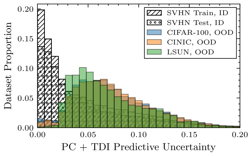
In the main paper, we have shown that PCs tend to be overconfident on OOD instances while PCs + TDI can overcome this challenge and can detect when an instance comes from a completely different distribution compared to what observed during training. This facilitates the separation between ID and OOD instances with a threshold, a peculiarity that is particularly useful also in practice in many domains. Here, we provide a complementary view of this ability of PCs with TDI. We show the predictive entropy in Fig. 6(a) and the predictive uncertainty in Fig. 6(b) obtained on the ID data and on several OOD datasets.

(a)

(b)

Figure 6: (6(a)) Histograms for the predictive entropy of PCs and PCs + TDI on ID (shaded) and OOD (colored) datasets in a classification context. PCs (left panel) assign similar, largely indistinguishable predictive entropy to OOD and ID data. In contrast, PCs + TDI (right panel) provides high uncertainty on OOD data, pushing the predictive entropy close to the obtainable maximum and effectively separating them from the known ID dataset. (6(b)) Predictive uncertainty (standard deviation as square root of Eq. 14) for the predictions provided by PC + TDI on ID (shaded) and OOD data (colored). Complementing the illustration of predictive entropy in (6(a)), the values support the picture that PCs + TDI are more unsure about OOD data and can thus make a distinction.

Appendix E PCs with TDI Are More Robust To Corruptions

We have applied 15 non-trivial natural and synthetic corruptions with respective five levels of severity, as shown in the main body’s experimental evidence section. For convenience, we re-iterate that the latter are commonly employed in the literature [Hendrycks and Dietterich, 2019] to test models’ robustness. More specifically, corruptions have been used to demonstrate standard neural networks’ inability to effectively handle corrupted data. Since we have observed an initial similar inability in PCs, they thus form a sensible test to evaluate the robustness of PCs versus PCs + TDI. To provide some visual intuition, a respective SVHN illustration is shown in Fig. 7.

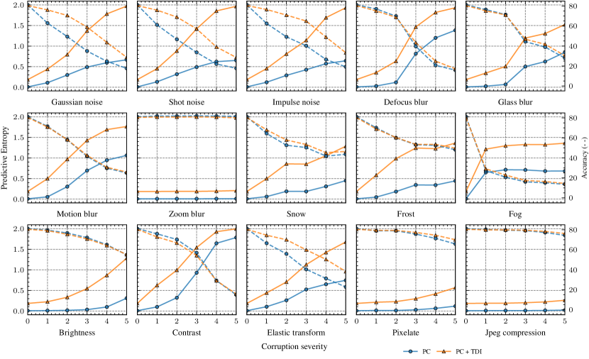
In our main body, we have shown the performance of PCs and PCs + TDI for 4 such corruptions and thus have provided empirical evidence for the robustness of PCs with TDI and their ability to attribute increased uncertainty to corrupted data. Here, we provide the full set of experiments for all 15 corruptions. Recall that for a model to successfully detect the corruption, it should assign a progressive increase in predictive entropy in accordance with the corruption severity.

The full quantitative results of Fig. 8 empirically affirm our conclusions drawn in the main body: PCs with TDI are generally equally or more robust at various severity levels for all corruptions, generally preserving equal or even higher predictive accuracy in several cases. At the same time, the assigned predictive entropy is substantially larger with an increasing level of corruption with TDI. Finally, we emphasize that in the three cases where PCs with TDI do not provide a large and successively increasing measure of entropy, i.e. zoom blur, pixelation, and jpeg compression, their respective accuracy in Fig. 8 is almost fully preserved. In other words, the model does not provide a large uncertainty because it already provides a correct and robust prediction.

Figure 7: Visual illustration of the 15 different corruptions with five increasing levels of severity as introduced in Hendrycks and Dietterich [2019] on an SVHN test sample.

Figure 8: Predictive entropy (left y-axis) and accuracy (right y-axis) of PCs (blue curve, circle markers) and PCs + TDI (orange, triangles) for increasingly corrupted SVHN data. 15 natural and synthetic corruptions are introduced at five severity levels. PCs with TDI can detect the distribution shift by assigning higher predictive entropy with increasing severity, while at the same time being more robust in predictive accuracy against the corruption, compared to PCs. We emphasize that in the three cases where PCs + TDI do not provide a large and successively increasing measure of entropy, i.e. zoom blur, pixelation, and jpeg compression, their respective accuracy (dashed) is almost fully preserved. The model is already correct and certain.

Appendix F Societal Impact

We believe that quantification of model uncertainty, as a direction to contribute to overall robustness, can have a broad positive societal impact. Colloquially speaking, an indication of when to “trust” the model is a valuable tool for users and practitioners, especially in safety-critical applications. That noted, gauging model uncertainty does not absolve users from careful considerations of other potentially harmful effects, particularly, the involvement of various forms of bias through training data, as these are then considered “certain” by definition.