Temperature dependence of fast relaxation processes in amorphous materials

Abstract

We examine the structural relaxation of glassy materials at finite temperatures, considering the effect of activated rearrangements and long-range elastic interactions. Our three-dimensional mesoscopic relaxation model shows how the displacements induced by localized relaxation events can result in faster-than-exponential relaxation. Thermal activation allows for local rearrangements, which generate elastic responses and possibly cascades of new relaxation events. To study the interplay between this elastically-dominated and thermally-dominated dynamics, we introduce tracer particles that follow the displacement field induced by the local relaxation events and also incorporate Brownian motion. Our results reveal that the dynamic exponents and shape parameter of the dynamical structure factor depend on this competition and display a crossover from faster-than-exponential to exponential relaxation as temperature increases, consistent with recent observations in metallic glasses. Additionally, we find the distribution of waiting times between activations to be broadly distributed at low temperatures, providing a measure of dynamical heterogeneities characteristic for to glassy dynamics.

I Introduction

When we rapidly cool down a metallic or polymeric melt to temperatures below the glass transition, the result is a highly viscous, heterogeneous and frustrated material that we call ‘amorphous solid’. Its non-equilibrium, topological and dynamical properties are part of one of the most salient open problems in Statistical Mechanics and, also, in Materials Science. From the viewpoint of the microscopic structure, some regions of the material freeze in states with high local stress barriers and others are more easily prone to relax since they correspond to soft regions close to instability. Although the material appears now solid on long time-scales and responds elastically to small deformations, it may still exhibit measurable internal relaxation dynamics. The relaxation process that develops and eventually alters the glass physical properties involves a wide range of time, energy and length scales, aging processes and sample preparation dependencies. Understanding this spontaneous aging is of key relevance in the attempts to control such mechanical degradation; for instance, to manage these materials in industrial applications. This makes it a relevant problem not only from a theoretical but also from a practical point of view.

The complexity of a quiescent glass relaxation is usually quantified by the way in which the so-called “dynamic structure factor” (viz. the intermediate scattering function) deviates from an exponential relaxation. In many cases, stretched exponentials are observed, possibly resulting from a broad distribution of relaxation times due to material heterogeneity. However, the opposite situation of ‘compressed’ relaxation (faster than the exponential) is also observed experimentally in various materials, such as metallic glasses or colloidal gels.

These compressed exponentials have recently been interpreted within a framework that puts forward the elastic response to local relaxation events in the material. The suggestion is that, even when the bulk material has an intrinsic elastic nature, the occurrence of localized and rather sparse relaxation events can be enough to modify and dominate the global relaxation behavior of the system. Each event leads to an elastic reponse of the sourrounding material and induces thereby a long range displacement field for the sourrounding particles. An experimental framework for the study of this unusual relaxation was first established by dynamic light scattering (DLS) works in fractal colloidal gels [1, 2, 3, 4, 5]. More recently, x-ray photon correlation spectroscopy (XPCS) has been used to study slow dynamics following the same spirit, but this time not only ‘soft’ materials as colloidal suspensions [6, 7], colloidal glasses [8] and gels [9, 10], but also in hard-amorphous materials such as metallic glasses (MGs) [11, 12, 13]. An overview of the state of the art by 2017 in physical aging and relaxation processes in MGs can be found in reference [14].

The structure factor in these experiments is extracted from the time-averaged temporal auto-correlation function of the scattered intensity $g^{(2)}(q,t)=\left<I(q,\tau)I(q,\tau+t)\right>/\left<I(q)\right>^{2}$ where $I(q,t)$ is the intensity of the signal measured with the corresponding scattering technique. $f(q,t)$ is related with $g^{(2)}$ through the Siegert relation

$$g^{(2)}(q,t)-1=\kappa|f(q,t)|^{2}\;.$$ (1)

The common feature observed in several experiments is a structure factor showing a compressed exponential behavior in time $t$ and scattering vector $q$ [4, 14]:

$$f(q,t)\sim\exp[-(t/\tau_{f})^{\beta}]\;,$$ (2)

with $\tau_{f}\sim q^{-n}$, $n\sim 1$ and $\beta>1$ . The observed dynamics was a priori unexpected, not only because of such a faster than exponential decay of the correlations but also because it contrasts with the usual diffusive behavior at long time-scales ($\tau_{f}\sim q^{-2}$) found in molecular dynamics simulations of most glassy systems. It should be mentioned that, although this measurements are performed in aging system, the compressed relaxation is not intrinsically an non-equilibrium feature. In general, experiments are focused in a time-window where the waiting time dependence can be disregarded, the age of the material can be considered fairly unchanged during the measurement. Moreover, cyclic shear experiments [15] showed that these compressed-exponential relaxation dynamics associated with ballistic-like motion is observed even in a well controlled stationary state. Note, that even in these examples of stationary dynamics a dynamical competition of time-scales remains present, that we show to be a possible origin of compressed exponential relaxation. In the stationary setup (without any applied deformation) thermal agitation causes Brownian motion of the individual particles within their cages and eventually local relaxation events are triggered by thermal activation. The elastic response to these events can induce further relaxation events, by destabilising new regions, that were already close to instability. Higher temperatures, not only induce more and more frequent relaxation events but also increase the diffusion of the particles. As we will discuss, the interplay between thermal Brownian motion and the persistent motion induced by elastic displacement fields due to localised relaxation events affects and quantitatively determines the relaxation process. In particular, this competition leads to an effectively temperature dependent exponent $\beta$ in the compressed exponential behavior of the dynamical structure factor $f(q,t)\sim\exp[-(t/\tau_{f})^{\beta}]$.

I.1 A literature overview

The idea that relates compressed exponential behavior of $f(q,t)$ with the elastic reponse to localized relaxation events events was introduced by Cipelletti et al. in [1]. It was later reformalized by Bouchaud & Pitard within in a mean-field scenario [16, 17, 18]. In [19] part of the authors of the present manuscript have proven this scenario valid in finite dimensions (2D) within simulations of a mesoscopic model for the relaxation dynamics of glassy materials. Although the local rearrangements leading to relaxation of the material are in general not individually assessed in the experiments, their relation with the compressed exponential behavior has been widely acknowledged.

Luo et al. [20] explored a wide temporal and temperature range in the relaxation of three typical Zr- and La-based metallic glasses (MGs). They directly measure the stress by applying a small tensile deformation on MG ribbons and follow its relaxation in time. They find a gradual change of the relaxation profile from a single-step to a two-step decay upon cooling. They relate the first faster relaxation process to the anomalous stress-dominated microscopic dynamics, and the secondary slower one, to subdiffusive motion at larger scales with a broader distribution of relaxation times. For this stress relaxation, they also observe compressed exponentials as soon as $T<0.9T_{g}$, where $T_{g}$ is the glass transition temperature.

In [21] Amini et al. studied structural relaxation a bulk metallic glass forming alloy. Upon heating across the glass transition, the intermediate scattering function (ISF) changes from a compressed to a stretched decay, with a smooth variation of the stretching exponent and the characteristic relaxation time. Authors relate this to a progressive transition between a stress-dominated dynamics of glasses and the mixed diffusion and hopping particle motion of super-cooled alloys. In this study compressed exponentials are observed bellow $T_{g}$, in agreement with  [11]. This is when the metallic alloy responds as an amorphous solid and localized relaxation events, akin to shear transformation zones (STZs) in sheared amorphous solids, can produce persistent displacements in their surroundings.

Interestingly, a very recent work by Song et al. [22] investigates again the kind of soft matter systems where compressed exponential relaxation were first reported. By analyzing microscopic fluctuations inside an arrested gel they differentiate among two distinct relaxation mechanisms: quiescent relaxations governed by the buildup of internal stresses during arrest, and perturbation-induced avalanche relaxation events governed by mechanical deformations in the system. In the quiescent case, when internal stress heterogeneities generated during arrest are released, they cause local strain propagation. In this gel these rearrangements caused by the pre-stressed states are even considered to be athermal, with an occurrence rate exceeding strongly the one of thermally activated rearrangements. XPCS on the arrested gel probed at quiescence shows a second-order correlation function $g_{2}(q,t)$ decaying as a compressed exponential function of $(q^{1.07}t)$ in a range of $q$ values, with a compressed exponent $\beta\sim 1.57$. The notion that intermittent plastic activity happens due to mechanical aging and relaxation of pre-stresses more than thermal activation, can be also found in metallic glasses [13].

Still, it should be also mentioned that not always the compressed exponent behavior is said to be related to relaxation of inner stresses. In ref. [23] the authors studied a system of polystyrene spheres in super-cooled propanediol. By means of multi speckle-dynamic light scattering experiments, at low temperatures, compressed exponential decays are observed. The speckle pattern shows indication for convection in the sample due to a slight temperature gradient across the sample cuvette mounted in a cold finger cryostat. Authors attribute the compressed exponentials to such convection, an effect that increases with decreasing temperature.

On the modeling side, the phenomenon of compressed exponential relaxation has also been discussed recently, both in the gel context as well as for hard amorphous materials. In a work on a gel created as a kinetically arrested phase separation it has been shown that its relaxation is accompanied by super-diffusive particle motion and compressed exponential relaxation of time correlation functions [24]. Spatiotemporal analysis of the dynamics reveals intermittent heterogeneities producing spatial correlations. Another work on gel relaxation in a network forming attractive gel showed similar behavior when local bond breakings were induced by hand [25]. The authors evidenced a cross-over of the shape exponent from compressed to stretched exponentials as a function of temperature pointing towards a competition between Brownian motion and elastic effects through the relaxation of internal stresses. On the metallic glass-former materials side, simulations in [26] showed that the relaxation dynamics is directly related to the local arrangement of icosahedral structures: Isolated icosahedra give rise to a liquid-like stretched exponential relaxation whereas clusters of icosahedra lead to a compressed exponential relaxation.

Recently, Ref. [27] revisited the idea of elastically interacting local relaxation events [1, 16] in an analytical atomistic approach, and discussed both slow stretched-exponential relaxation and fast compressed-exponential relaxation; the latter being related to the ‘avalanche-like dynamics’ in the low-temperature glass state. Based on Arrhenius-type activation of stress-relaxation events, similar to the work in ref. [19], their model, already at the mean-field or ‘one-site’ approach, evidences a temperature dependency in both the stretched and compressed behavior regimes.

I.2 Our work

In this work, we first confirm through the numerical study of a simple three dimensional lattice model that compressed exponential relaxation can result from elastic relaxations responding to thermally induced local rearrangements akin to shear transformations observed in yield stress materials with external driving [28, 29, 30].

We use a three-dimensional elasto-plastic model of amorphous solids (described in Sec. III) together with the construct of imaginary tracer particles evolving in parallel. These particles follow the vector displacement field generated by the elasto-plastic model, associated with the stress response to the thermally induced plastic activity of the modeled material. The particle trajectories are then used to calculate both the mean square displacement and the dynamical structure factor.

Our results show that for sufficiently short times there is a super-diffusive regime in the mean square displacement of tracer particles, after which we enter a crossover regime towards diffusive behavior. Note that we refer to short and long times here within our coarse-grained elasto-plastic description . The crossover is dominated by the typical duration of plastic events. In addition, a compressed exponential relaxation, reminiscent of experimental observations, is obtained in the dynamic structure factor associated with the super-diffusive (ballistic-like) regime. At long times, in the diffusive regime, the relaxation is instead exponential. Furthermore, we analyze in more detail the relaxation dependency on the temperature. The presence of finite temperature that allows for the activation of plastic events, also generates thermal agitation that competes with the persistent movement on short times [25]. We observe that temperature modifies the crossover between super-diffusive and diffusive motion and effectively generates an intermediate range of values for the exponent $\beta$ of the structure factor decay. Hence, our model allows for a theoretical interpretation of recent observations in metallic glasses [32, 21]. We discuss this phenomenology presenting results and scaling laws for the mean-square displacements $\left<r^{2}\right>$ of tracer particles, the displacement distributions $P(u)$ in different time windows, the distributions of reactivation times of local plastic activation $\Psi(\tau_{\tt re})$ and the dynamical structure factor evolution $S(t)$.

Originally inspired in the dense phase of athermal amorphous materials, elasto-plastic models [33] are not a priori expected to capture the physics of the glass transition. Yet, building on the idea that highly viscous liquids should be considered as “solids which flow” [34, 35, 36], recent endeavors have revealed that simple EPMs with thermal activation of plastic events are able not only to reproduce compressed exponential relaxation [19], but also other features of glassy dynamics, such as dynamical heterogeneities and the emergence of dynamical correlations [37], precisely due to the mediation of elastic interactions in the material. Within this context it seems thus justified to argue that the low temperature limit of our model mimics reasonable well the relevant relaxation processes in the low-$T$ phase of glass-forming liquids. In this picture relaxation is dominated by displacement fields rooted in elasticity and local rearrangements. At higher temperatures it is the increasing Brownian motion of particles that leads to the breakdown of the elasto-plastic picture, localisation and activatation, the main features of glassy glassy dynamics, become more and more irrelevant and we enter the dynamics of high-temperature super-cooled liquids.

The next Section II is a summary of the mean-field arguments for the elasticity-mediated compressed exponential phenomenon. Although important for the general understanding of the importance of elasticity in the relaxation processes, this part is not directly needed to access the main part of this manuscript describing our work on the spatially-resolved elasto-plastic modeling.

In Section III we present our elasto-plastic model and the construction of thetracer particles for the particle displacements. Section IV presents our findings and we conclude in Section V.

II Recall of mean field arguments

In [1] an heuristic explanation for the phenomenon of compressed exponentials was first introduced, based on the “syneresis” of a gel. Syneresis is a spontaneous contraction of a gel, which occurs locally, accompanied by expulsion of liquid from a pore. The gel shrinks. Such mechanical inhomogeneities act as local dipole forces with a long range elastic impact on its surroundings, creating a complex deformation field [1]. The argument leading to the justification of a compressed exponential observation in the dynamical structure factor goes as follows.

The displacement field $u$ due to an inhomogeneity (a syneresis event) at a distance $r$ goes as

$$u\sim\epsilon(t)V_{1}/r^{d-1}$$ (3)

where $V_{1}$ is an estimate for the volume of the region involved in the syneresis, $\epsilon(t)$ is the evolving strain on that region, and $d$ is the dimension of the system. If the inhomogeneity is placed at the origin, the generated displacement field decays algebraically. The observable that we are interested in measures spatial correlations at two different times, an corresponds to an overlap function.

Figure 1: Schematic figure that shows that given a spatial configuration of particles ($t=0$), if the particles move the structure factor decays until this system decorrelates the initial condition in a time $t$. (adapted from a slide by B. Ruta)

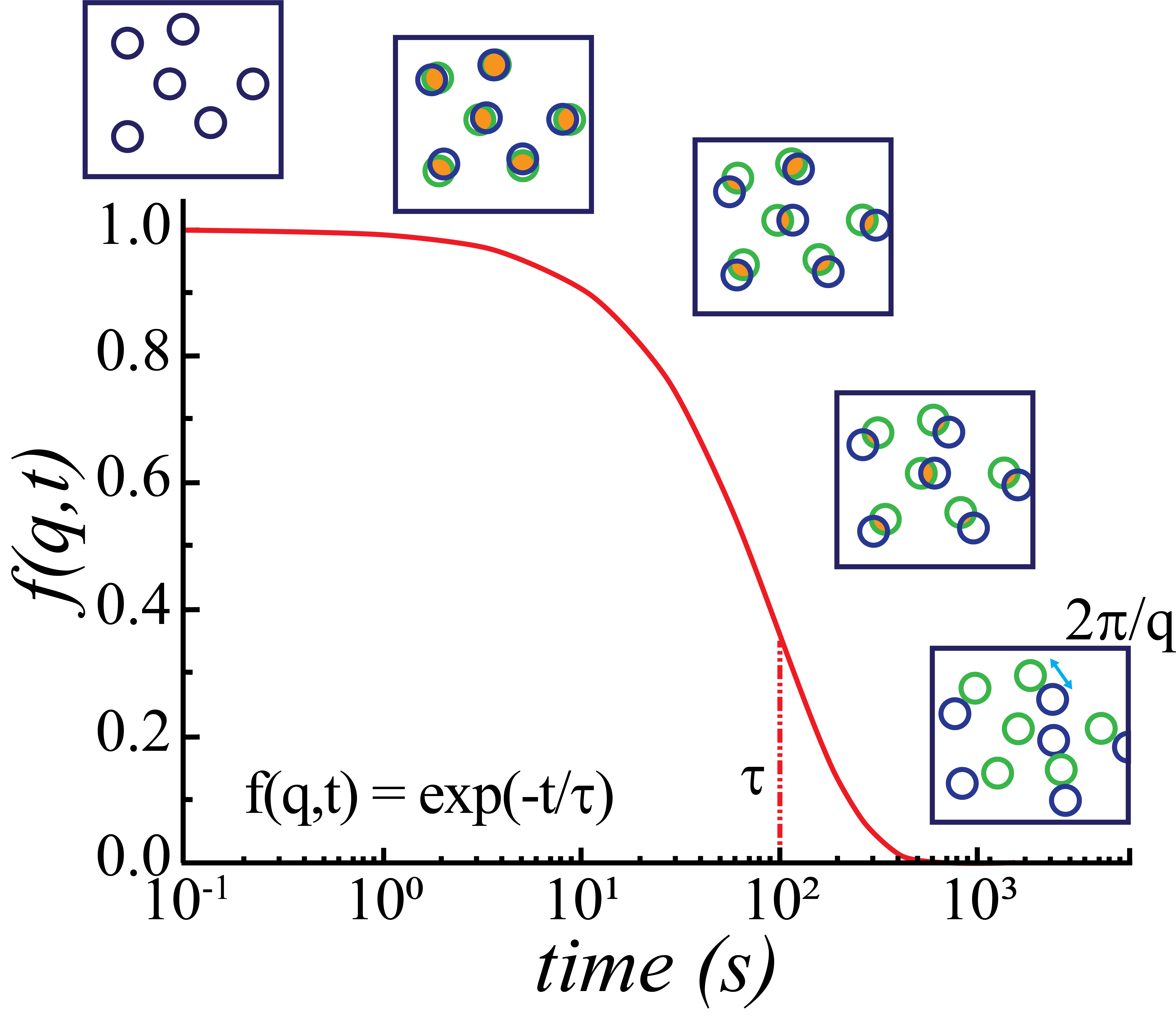
Given an initial configuration of particles, as depicted in Fig. 1, the structure factor $f(t,q)$ would stay close to $f(t=0,q)=1$ if the particles don’t move, and will drop all the way down to $0$ if the configurational correlation with the initial condition is completely lost at time $t$. Due to the intensity decay of the displacement field, the particles closer to the inhomogeneity will move stronger and lead to a strong decrease of the spatial correlations. If we are observing the system at a typical space resolution of $q^{-1}$ (akin to using light scattering techniques with a wavevector of modulus $q$) and we ask for $u<q^{-1}$ to consider that something has basically ‘not moved’ at that length-scale, we need it to be at a distance to the closest dipole equal or larger than

$$r_{\tt min}\simeq\left[q\Delta_{\epsilon}(t)V_{1}\right]^{\frac{1}{d-1}}.$$ (4)

This simply accounts to inverting eq.3 and introducing $\Delta_{\epsilon}(t)\simeq q^{-1}\epsilon(t)$, as a measurable linear displacement. The distance to the closest dipole will depend on the density of syneresis events. Assuming an inhomogeneity concentration $c$ in a system volume in dimension $d$, we can expect the probability of being further than a distance $r_{\tt min}$ to any inhomogeneity to decay as

$$P(r_{\tt min})\simeq\exp\left[{-cr_{\tt min}^{d}}\right]\simeq\exp\left[{-c\left[q\Delta_{\epsilon}(t)V_{1}\right]^{\frac{d}{d-1}}}\right].$$ (5)

Notice that, $P(r_{\tt min})\equiv P_{r_{\tt min}}(q,t)$ is already a good proxy for $f(q,t)$, since higher probability of being away from any strong field distortion means higher preservation of correlation at a given time. So one can propose $f_{\tt mf}(q,t)\propto P_{r_{\tt min}}(q,t)$, and assuming that the local strain within the inhomogeneity varies linearly in time $\epsilon(t)\simeq at$ we get

$$f_{\tt mf}(q,t)\propto\exp\left[-(t/\tau_{r})^{d/(d-1)}\right]$$ (6)

with $\tau_{r}=c^{-(d-1)/d}(V_{1}aq)^{-1}$ emerging as a characteristic relaxation time. Notice that $\tau_{r}\propto q^{-1}$, which is typical of a persitent motion. Generalizing Eq. 6 to three dimensions ($d=3$) we have

$$f_{\tt mf}(q,t)\propto\exp\left[-(t/\tau_{r})^{3/2}\right]$$ (7)

which is already giving a possible explanation for the commonly seen exponent $\beta\simeq 3/2$ fitted from experimental data when assuming compressed exponential decay in time of $f_{\tt mf}(q,t)$.

This idea was taken by Bouchaud & Pitard to build a mean-field model to predict the anomalous relaxation phenomenon [16, 17, 18]. They have taken into account that the local deformation stops at some point and included a new relevant time scale $\theta$, corresponding to the duration of a plastic rearrangement. They analytically compute

$$f_{\tt mf}(q,t)=\left<\exp\left[i\mathbf{q}\cdot(\mathbf{u}(\mathbf{r},t_{0}+t)-\mathbf{u}(\mathbf{r},t_{0}))\right]\right>$$ (8)

and extract the relevant regimes

$$f_{\tt mf}(q,t)\propto\begin{cases}\exp[-a_{b}(qt)^{3/2}]&\text{if $t\ll\theta$}\\ \exp[-a_{d}(q^{3/2}t)]&\text{if $t\gg\theta$}\end{cases}$$

where $a_{b}$ and $a_{b}$ are constants. The $q^{3/2}$ dependence reflects the fact that the distribution of local displacements $u$ decays as $u^{-5/2}$ and therefore has a diverging variance [18]. One can see that in the case of very high plastic activity (or temperature), the $P(u)\sim u^{-5/2}$ heavy tail is always suppressed, and therefore we recover the usual $q^{2}$ dependence in the diffusive regime.

Notice that the mean-field description of Bouchaud & Pitard [16] always predicts a purely ballistic-like scaling between space and time $q^{-1}\propto t$ in the regime where correlation functions decay as compressed-exponentials. Further, the presented mean-field approach predicts no temperature- or $q$-dependency for the compressed exponent. In experiments however, temperature- or $q$-dependency are commonly reported and two clear trends appear in the experimental literature:

(i) On one hand, frequently a $q$-dependence of $\beta$ is reported [5, 38, 39, 6, 11, 12] and along with that the $q^{-1}\propto t$ relation is broken. In particular, the physics is better described by [6]

$$f(q,t)\propto\exp\left[-c(q^{\alpha}t)^{\beta}\right].$$ (9)

Clearly, spatial correlations among plastic events play a role in the relaxation dynamics. Already, an improvement in theoretical predictions is seen when intermittency of plastic events is taken into account (versus a continuous ballistic process). In [5], Duri et al. showed that a model of intermittent dynamics can predict a $q$-dependency of $\beta$. Using a Poisson distribution for $P_{\tau}(n)$, the probability that $n$ plastic events affect the scattering volume during a time span $\tau$, they are able to justify their observation of a $\beta$ ranging from from $1.5$ to $1$ in the dynamic light scattering of a colloidal gel for increasing $q$. The variation of $\beta$ with $q$ was also observed at low temperatures in glass forming liquids [6].

(ii) Another ubiquitous observation is the dependency of the shape exponent $\beta$ with temperature [6, 32, 20, 21]. It has been seen that $\beta$ decreases systematically as temperature is increased. Furthermore, in [32, 21] it’s suggested that the compressed-exponential behavior of $f(q,t)$ is lost when approaching the glass transition temperature $T_{g}$ estimated from calorimetric measurements of the metallic glasses alloys. Although it’s intuitive to assume that the melting of the material leads to a loss of the solid support and therefore elastic perturbations induced by localised plastic events cease to exist, it might not be the only reason for loosing the compressed-exponential behavior. For instance, thermal agitation could start being relevant much before the melting of the glassy mixture, and, on the other hand, there are numerical evidences for the subsistence of Eshelby events in the super-cooled liquid phase [40, 28, 41].

In fact, the temperature-dependency of the relaxation remains an open issue on the theoretical side. It has not been discussed in the previously quoted mean-field-like approximations, and only recently included in a related analytical approach [27]. We address such an elasticity-temperature interplay in the present work in a fully spatial description.

III Model

In the last decade, different coarse-grained approaches have been developed to help in the understanding of amorphous solids under deformation [33]. Such lattice-based models known as “elasto-plastic” (EP) have the advantage of being capable to address larger scale statistics of the dynamical phenomena related with plastic deformation in amorphous solids, than the one provided by (more “realistic”) off-lattice particle-based models. If we want to describe a material with a given extension and in a given time-frame, the computational demand is, of course, much larger for a particle based approach. The coarse-graining solves that, allowing us to address length and time scales that involve several shear-transformation-zones (STZ) to study their interplay and statistics.

Yet an automatic drawback of EP models is the absence of “particle coordinates”, from which many common observables are usually defined. By construction, EP blocks are supposed to describe a region or patch of the material, involving several particles, where a STZ or “plastic event” can take place. A way overcome this limit, while still keeping the enormous functionality of EP models in the statistical description of amorphous materials is to construct a parallel system of lattice-free tracer particles. These point-like particles will follow the instantaneous displacement fields derived from the EP-model, and provide us with virtual particle-coordinates and configurations that we can use to define quantities as the mean-square-displacement and the dynamical structure factor. Assuming that localized relaxation events perturb the surrounding material leading to a stress redistribution in form of an Eshelby response, one can convolute the simultaneous action of several plastic events occurring in different locations to workout the displacement field ${\bf u}({\bf r})$ that they induce at any place in the system. Of course, the resolution of the corresponding displacement field is given by the coarse-graining of the elasto-plastic lattice dynamics, but once we derived it we can ignore the the lattice for the movement of tracers. This construction was used in [19] for the study of a 2D system; we extend it here to the case of three dimensions and add a thermal noise to the dynamics of tracers in a way fully compatible with thermal activation of plastic events in the background EP model.

A thermally activated and spatially symmetrized elasto-plastic model

An amorphous material is represented by a coarse-grained scalar stress field $\sigma({\bm{r}},t)$, at spatial position ${\bm{r}}$ and time $t$ under an externally applied shear strain. The space is discretiszd in patches or blocks. At a given time, each block can either be elastic (“inactive”) or plastic (“active”, i.e., locally relaxing). This state is defined by the value of a binary variable: $n({\bm{r}},t)=0$ for inactive, $n({\bm{r}},t)=1$ for active. A huge model simplification consist in passing from a fully tensorial description to a scalar one, for example, by assigning all the plastic deformation to one scalar component of the deviatoric strain. While this approach is analytically justified in the case of sheared materials (e.g., [42]), we would need here to take into account the tensoriel caracter since we do not have any symmetry-breaking external applied deformation. To be able to keep a simple scalar description, we decided to symmetrize the reponse in the three possible shear ‘directions’, not favoring one spatial coordinate over the others.

We define our EP model in $3$-dimensions discretized on a cubic lattice of $N=L_{x}\times L_{y}\times L_{z}$ blocks, with the stress $\sigma_{i}$ on a generic block $i$ subject to the following evolution in real space

$$\frac{\partial\sigma_{i}(t)}{\partial t}=-g_{0}n_{i}\frac{\sigma_{i}(t)}{\tau}+\sum_{j\neq i}G_{ij}n_{j}(t)\frac{\tilde{\sigma}_{j}(t)}{\tau};$$ (10)

where $g_{0}>0$ sets the local stress dissipation rate for an active site, the time-dependent local state variable $n_{i}=\{0,1\}$ indicates if a site is undergoing a plastic event (active ($n_{i}=1$) or inactive ($n_{i}=0$)), and the kernel $G_{ij}$ is the Eshelby stress propagator [43]. In most EPMs, ${\tilde{\sigma}_{j}(t)}$ is simply ${\sigma}_{j}(t)$, the stress at site $j$. Yet, in this case we have used $\tilde{\sigma}_{j}(t)=\pm\mu\epsilon_{0}$, where the sign ($\pm$) indicates whether the plastic activation has occurred in a positive ($+$) or negative ($-$) stress threshold and $\epsilon_{0}$ quantifies a fixed intensity for the Eshelby event during the plastic event. This our choice for ${\tilde{\sigma}_{j}(t)}$ is justified in a subsection below. Furthermore, notice that typically a $\mu\dot{\gamma}^{\tt ext}$ term (with $\mu$ the shear modulus and $\dot{\gamma}^{\tt ext}$ the externally applied strain rate) appears in the R.H.S., but in our case it’s identically zero (no external driving).

The form of $G$ in $d=3$ can be more easily expressed in Fourier space

$$G_{\bf q}^{\tt 3D}=-\frac{4q_{l}^{2}q_{m}^{2}+q_{n}^{2}(q_{l}^{2}+q_{m}^{2}+q_{n}^{2})}{(q_{l}^{2}+q_{m}^{2}+q_{n}^{2})^{2}}$$ (11)

for $\bf q\neq 0$ and, in our scheme of non-conserved stress,

$$G_{\bf q=0}=-\kappa$$ (12)

with $\kappa$ a numerical constant set to 1. The sub-indices $l,m,n$ of the wavevector $\bf q$ components in Eq. 11 are set to different possible permutations of the system coordinates $x,y,z$, as explained later. The last term of (10) constitutes a mechanical noise acting on $\sigma_{i}$ due to the instantaneous integrated plastic activity over all other blocks ($j\neq i$) in the system. The elastic (e.g. shear) modulus $\mu=1$ defines the stress unit, and the mechanical relaxation time $\tau=1$, the time unit of the problem.

The thermal activation rule

The picture is completed by a dynamical law for the local state variable $n_{i}=\{0,1\}$. In the athermally driven case, a plastic event occurs in block $i$ ($n_{i}:0\rightarrow 1$), with certain probability [44], when the local stress $\sigma_{i}$ overcomes a local yield stress ${\sigma_{\tt Y}}_{i}$. In the current work, the driving is absent and is replaced by thermal activation. When $T>0$ we expect activation to occur with a finite probability even if $|\sigma_{i}|<{\sigma_{\tt Y}}_{i}$, where now we should equally consider the probability of yielding when a block builds a sufficiently large ‘negative’ stress. In particular, we use the following rule for sites activation: $n_{i}:0\rightarrow 1$ as soon as $|\sigma_{i}|\geq{\sigma_{\tt Y}}_{i}$, or, at any time with probability

$$p_{\tt act}(T)=e^{-B({\sigma_{\tt Y}}_{i}-|\sigma_{i}|)^{\alpha}/k_{B}T}$$ (13)

when $|\sigma_{i}|<{\sigma_{\tt Y}}_{i}$ . We have chosen for simplicity ${\sigma_{\tt Y}}_{i}=1$ for all sites (and $k_{B}=1$). We checked that the use of distributed stress thresholds does not change qualitatively our findings. The factor $B$ can be seen as a measure of facilitation of local slips and therefore considered a material-dependent parameter. In our model, it remains a free parameter that we control. In the following we set $\alpha=3/2$, taking into account the discussion in [44, 46] which identifies it as the exponent expected for smooth energetic barriers and the most comparable one with atomistic simulations and experiments . Finally, an active block $i$ becomes inactive $n_{i}:0\leftarrow 1$ with a constant probability $\tau_{\tt ev}^{-1}$. The prescribed time $\tau_{\tt ev}$ is the ‘lifetime’ of an active event and the previous stochastic rule guarantees that, on average, plastic events have such a duration. The value for $\tau_{\tt ev}$ is also not fixed and remains a free model parameter.

Symmetrized elastic propagator and strain events

In the absence of an external shear, there’s no preferred direction for an Eshelby event. In principle we should consider that the local shear transformations occur arbitrary orientations and angles. This apparently ingenuous statement can largely complicate the numerical implementation of the model and it’s unnecessary for our purposes. Even though a bit less realistic, for simplicity we have chosen to preserve the symmetry only between the three principal shear planes of our $d=3$ sample geometry ${xy},{yz},{zx}$. We define not one but three different propagators related to these shear planes: Eq. 11 with three index permutations for $(l,m,n)$: $(x,y,z)$, $(y,z,x)$ and $(z,x,y)$. When the criterion for local yielding is met, one shear plane is chosen randomly and that site will be shear-transforming in that orientation only during it’s activity period. The next activation of the same site can occur in a different orientation. In this way we maintain a single local scalar variable representing the stress on each block, despite the introduction of various possible orientations of a plastic event. Moreover, the absence of an externally applied shear restrains the system to plastic activity only induced trough a ‘thermal bath’. Local stresses are close to Gaussian-distributed around zero and the width of the distribution increases with $T$ (see App. A). In a sense, our system enters after a transient dynamics depending on the initial state, always in thermal equilibrium. In the absence of externally applied deformation, we associate to a plastic event a characteristic strain rather than a characteristic stress [19] as is usually the case for EPMs with driven dynamics. As mentioned, in practice $\tilde{\sigma}_{j}(t)$ in Eq.(10) is defined as

$$\tilde{\sigma}_{j}(t)=\pm\mu\epsilon_{0},$$ (14)

if the site is active, where the sign ($\pm$) depends on the plastic activation occurring at a positive ($+$) or negative ($-$) stress threshold. $\epsilon_{0}$ constitutes a parameter of our model and quantifies the intensity of the Eshelby event; it can be seen as the $\epsilon V_{1}$ in Eq.(3).

Displacement fields and tracer particles

The yielding of a block in different shear planes will give rise to displacement fields in the rest of the system, which we capture using the Oseen tensor components, following and generalizing [43]. In Fourier space

$$\hat{{\bf u}}({\bf q})=\hat{\mathbf{O}}({\bf q})\cdot(2i\mu{\bf q}\cdot\hat{{\bf\epsilon}}_{\tt pl})$$ (15)

${\bf u}({\bf r})$ (the real-space counterpart of ${\bf u}{(\bf q})$) is the vectorial displacement field, ${\bf\epsilon_{\tt pl}}({\bf r})$ is a plastic strain shear-component ($\epsilon_{\tt pl}{}_{j}=n_{j}\tilde{\sigma}_{j}/\mu$, the strain related to the stress multiplying the propagator in Eq. (10)), and $\mathbf{O}({\bf r-r^{\prime}})$ is the translationally-invariant Oseen tensor.

$$\hat{\mathbf{O}}({\bf q})=\frac{1}{\mu q^{2}}\left(\mathbf{I}-\frac{{\bf q}{\bf q}}{q^{2}}\right)$$ (16)

Given an instantaneous configuration of the system’s plastic activity (with its complexity of three possible local yielding directions for each block), one can convolute the different contributions given the active blocks to the displacement field at any position in the system by using Eq.(15) in Fourier and then transforming ${\bf u}{(\bf q})$ to real space. Here we consider for the shear components of $\hat{\mathbf{O}}({\bf q})$ the same three possible permutations that we used for the propagator $G_{\bf q}$. Notice that for a more detailed description one would need to be careful about the displacements in an event’s core region, which follow a different (exponential) decay [48]. Here we had simply taken the precaution of setting things such that a plastic event has a null effect in the displacements of tracers that are transiting its own cell and only affect the tracers outside the event’s core.

With this, tracer particles are simulated in parallel to our EP model evolution, simply following the displacements fields. A set of $M$ probe particles initially located at random in the cube $(L_{x},L_{y},L_{z})$ simply follow the EP-model-generated displacement fields updating the position ${\bm{\xi}}_{s}$ for tracer $s$ by

$${\bm{\xi}}_{s}\to{\bm{\xi}}_{s}+\mathbf{u({\bm{\xi}}_{s})}dt$$ (17)

on its three scalar components. We call these ‘athermal tracers’, since temperature does not step in explicitly in their dynamics. This is modified in Sec. IV.2 when we include a thermal noise acting on the tracers.

From the movement of these tracer particles we will compute most of our quantities of interest. In a real system, the particles that we observe are in general not tracers but the system constituents themselves. Therefore, for example, dilation occurring inside the STZs will contribute to particle displacements [49]. Our approach disregards those contributions and takes only into account displacements generated by the long-range elastic response.

IV Results

Figure 2: Mean square displacement as a function of observation time window. The main plot shows the MSD $\left<r^{2}\right>$ rescaled by the mean activity $\left<a\right>$ for seven different activities/temperatures as indicated in the labels, The gray solid and dashed lines are guidelines to show the ballistic ($\sim t^{2}$) and diffusive ($\sim t$) behaviors. The inset shows $\left<r^{2}\right>$ unscaled. The plastic events duration is $\tau_{\tt ev}=1.5$. $\epsilon_{0}=1.0$. $L=32$.

In this section we present the numerical results for the relaxational dynamics of our quiescent EP model at finite temperature. All results correspond to steady-states, which due to the absence of external driving can be considered as being equilibrium states, as discussed in [19]. In a real material at rest (quiescent), the plastic activity might decrease (and even stop at some point) when the residual stresses of the material preparation are exhausted. Here, we perform measurements at fixed temperatures or fixed plastic activity levels and do not consider any material aging in the long term. We therefore expect our results to be comparable to the cases in which a given level of plastic activity is maintained in experiments or atomistic simulations during the measurements.

IV.1 Thermally induced plastic events for ‘athermal’ tracers

We start by discussing the extension to three dimensions of the results presented in [19]. A finite temperature rules the rate of plastic activity resulting in displacement of tracer particles, but those tracers move just according to the displacement fields without any other perturbing force.

IV.1.1 Mean square displacement

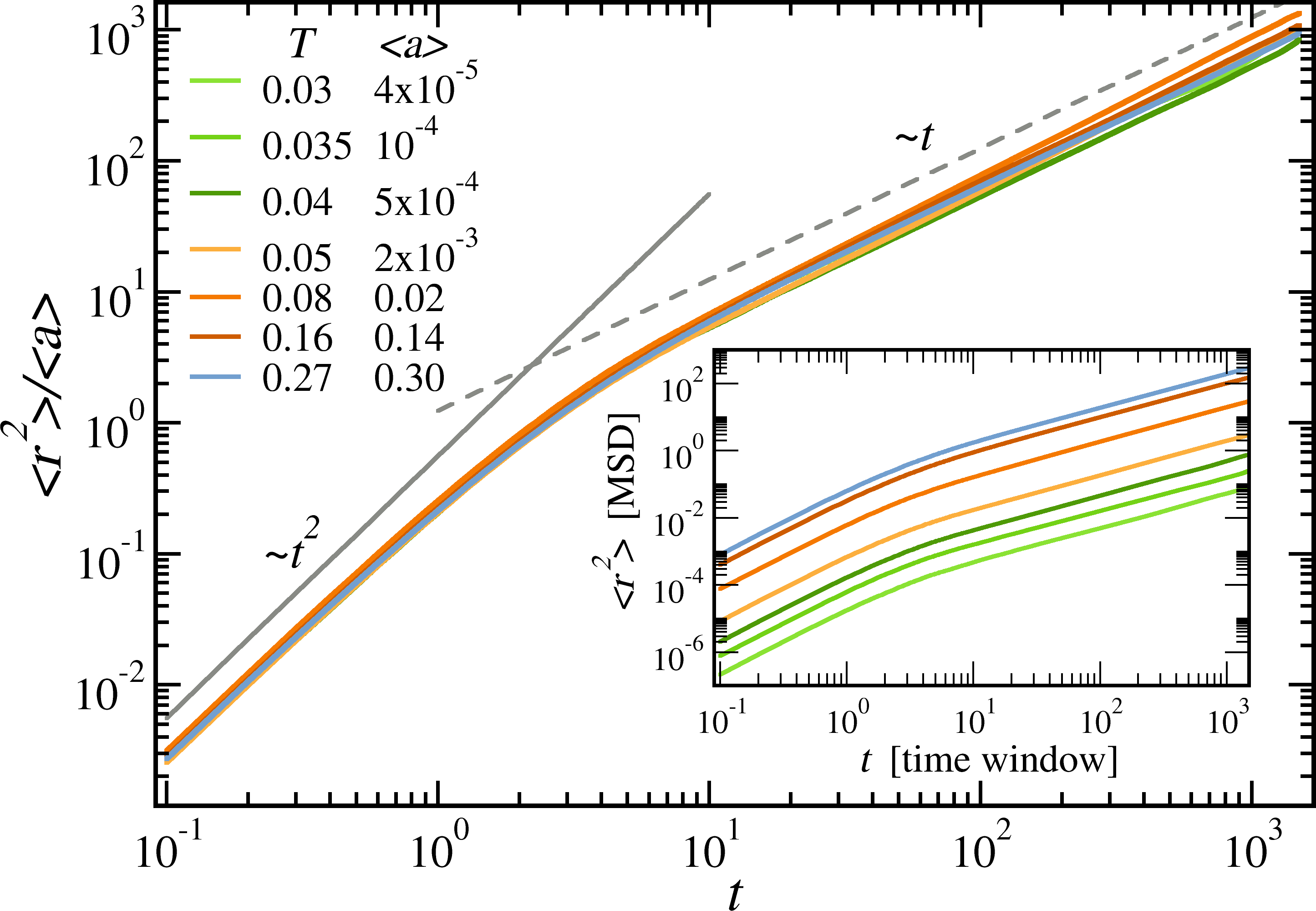
Figure 2 shows for different temperatures the mean square displacement (MSD) defined as $\left<r^{2}\right>~{}\equiv~{}\overline{\frac{1}{N}\sum_{i}r^{2}_{i}}$, where $r_{i}~{}=~{}|{\bf r}_{i}(t_{0}+t)-{\bf r}_{i}(t_{0})|$ is the distance traveled by tracer $i$ in the time-lapse $t$ and the over-line indicates an extra average using sliding time windows, by moving $t_{0}$ in the stationary state. Tracer particles move following the vector displacement field ${\bf u}(r,t)$ (Eq. 15). Data corresponds to cases of seven different mean plastic activities $\left<a\right>\simeq[4\!\times 10^{-5},1\!\times 10^{-4},5\!\times 10^{-4},2\!\times 10^{-3},0.02,0.14,0.3]$ resulting from temperatures $T\simeq[0.03,\,0.035,\,0.04,\,0.05,\,0.08,\,0.16,\,0.27]$, respectively, and $B=1$. For a given temperature, we observe that $\left<r^{2}\right>$ behaves ballistic-like ($\sim t^{2}$) if the time window observation is small, and, diffusively ($\sim t$) for larger time windows. The characteristic time scale separating this two regimes is the duration of the plastic events $\tau_{\tt ev}$ (which for data in Fig. 2 is $\tau_{\tt ev}=1.5$). What is identified as “ballistic” here is nothing but a regime dominated by the persistent motion of tracer particles during the elastic response in a given direction each, with little or none deviation. Beyond the persistent time controlled by $\tau_{\tt ev}$, particles diffuse. As expected, larger plastic activities lead to larger plastic displacements and larger effective diffusion coefficients $D_{\tt eff}\equiv\frac{\left<r^{2}\right>}{6t}$ at long $t$. In the main-plot of Fig. 2 we are able to collapse all curves when normalizing the MSD by the mean plastic activity $\left<r^{2}\right>/\left<a\right>$, where $\left<a\right>=\left<\frac{1}{N}\sum_{i}n_{i}\right>$ and $\left<\cdot\right>$ denotes average over time.

It’s worth clarifying something again about the persistent regime observed here. In the relaxation of glasses, a so-called $\beta$ relaxation takes place first, inside the cages formed by the frustrated material. At times smaller than the beta relaxation time the mean-square displacement can display a true ballistic regime where particles move freely within their cage. EPMs do not catch such a microscopic dynamics, they are defined at a mesoscopic level. All the relaxation presented in this work should be related to a relaxation occurring far beyond the $\beta$ relaxation, at much larger time and length scales. The tracer displacements we consider are the result of the elastic response to plastic events that in real systems can involve up to a few dozens of particles. As already suggested in [19], we believe that the EPM approach catches the relevant length scales where compressed relaxation is observed in experiments. And by that we mean the regime of wave vectors comparable to the typical core size of a local relaxation event in the material and at times related to the typical duration of those events.

IV.1.2 Dynamical structure factor

Figure 3: Dynamical structure factor $S(q,t)$ relaxation for low plastic activity and short times (in the ballistic regime). The inset shows $S(q,t)$ as a function of $q^{2}$ for time windows up to $t=100$, while the duration of plastic events is $\tau_{\tt ev}=20$. The mainplot collapses the curves corresponding to time-windows $t\leq\tau_{\tt ev}$, plotting $S(q,t)$ as function of $q^{1.1}t$. A compressed exponential behavior $S(q,t)\propto\exp\left[-A(q^{1.1}t)^{\beta}\right]$ is fitted with $\beta\simeq 1.58$ (blue curve). $T=0.02$. $\epsilon_{0}=0.1$. $L=32$.

We further compute the main observable of the relaxation dynamics, the dynamical structure factor $S(q,t)$, analogous of Eq. 8:

$$S(q,t)=\frac{1}{M}\left\langle\sum_{n=1}^{M}\cos\left[\mathbf{q}.\left(\mathbf{r}_{n}(t+t_{0})-\mathbf{r}_{n}(t_{0})\right)\right]\right\rangle,$$ (18)

which is a measure of the decorrelation of tracer particles positions in time respect to an initial configuration. Here $M$ is the total number of tracer particles, and the brackets indicate a sliding time-window average with different $t_{0}$ and the different discretized wave vectors $\mathbf{q}$ that share the same modulus $q$. In fact, we find it easier to get averaged curves at fixed times $t$ rather than at fixed $q$ values. It’s worth mentioning that although we are computing a self-ISF in the definition of Eq.(18), from tracers that do not interact with each other, they all follow displacement fields that are a result of the collective behavior of plastic events .

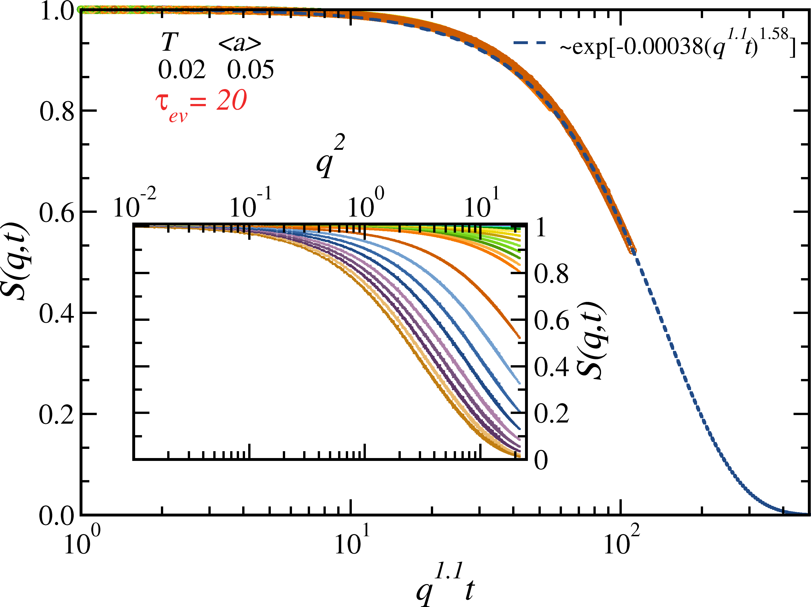
Figure 3 shows the dynamical structure factor for curves corresponding to short times ($t\lesssim\tau_{\tt ev}$). This means that the data displayed is collected from the persistent tracer movement regime. To observe such regime clearly we have set a large event duration, $\tau_{\tt ev}=20$, which in turn enforces a reduction of the parameter $\epsilon_{0}$ in Eq.14 in order to maintain the mean activity at low levels ($\left<a\right>=0.05$). Here $\epsilon_{0}=0.1$ has been used. A collapse of different curves can be seen when we plot $S(q,t)$ vs $(q^{1.1}t)$, and $S(q,t)$ presents the shape $S(q,t)\!\propto\!\exp\left[-A\left(q^{\alpha}t\right)^{\beta}\right]$, with $\alpha\simeq 1.1$, $\beta\simeq 1.58$. In this short time regime therefore we observe: (i) $\tau_{r}\sim q^{-1}$, typical of ballistic processes, and (ii) a compressed shape exponent $\beta$ in the range expected from experiments [51] and close but different from mean-field theory [16, 18].

Figure 4: Dynamical structure factor $S(q,t)$ relaxation for low plastic activity and long times (in the $q^{3/2}t$ diffusive regime). The lower-inset shows $S(q,t)$ as a function of $q^{2}$ for time windows up to $t=10000$. The duration of plastic events is $\tau_{\tt ev}=1.5$. The mainplot and upper-inset collapse the curves corresponding to time-windows $\tau_{\tt ev}\leq t\leq 1000$, plotting $S(q,t)$ as function of $q^{3/2}t$. A pure exponential behavior $S(q,t)\propto\exp\left[-A(q^{3/2}t)\right]$ is fitted. $T=0.04$. $\left<a\right>\simeq 0.0005$. $\epsilon_{0}=1.0$. $L=32$.

Figure 5: Dynamical structure factor $S(q,t)$ relaxation for moderate/high plastic activity and long times (in the usual $q^{2}t$ diffusive regime). The lower-inset shows $S(q,t)$ as a function of $q^{2}$ for time windows up to $t=1000$. The duration of plastic events is $\tau_{\tt ev}=1.5$. The mainplot and upper-inset rescale the curves corresponding to time-windows $t>20$ (curves on the left of the dark-orange one in the inset), plotting $S(q,t)$ as function of $q^{2}t$. A pure exponential behavior $S(q,t)\propto\exp\left[-A(q^{2}t)\right]$ is fitted. $T=0.16$. $\left<a\right>\simeq 0.14$. $\epsilon_{0}=1.0$. $L=32$.

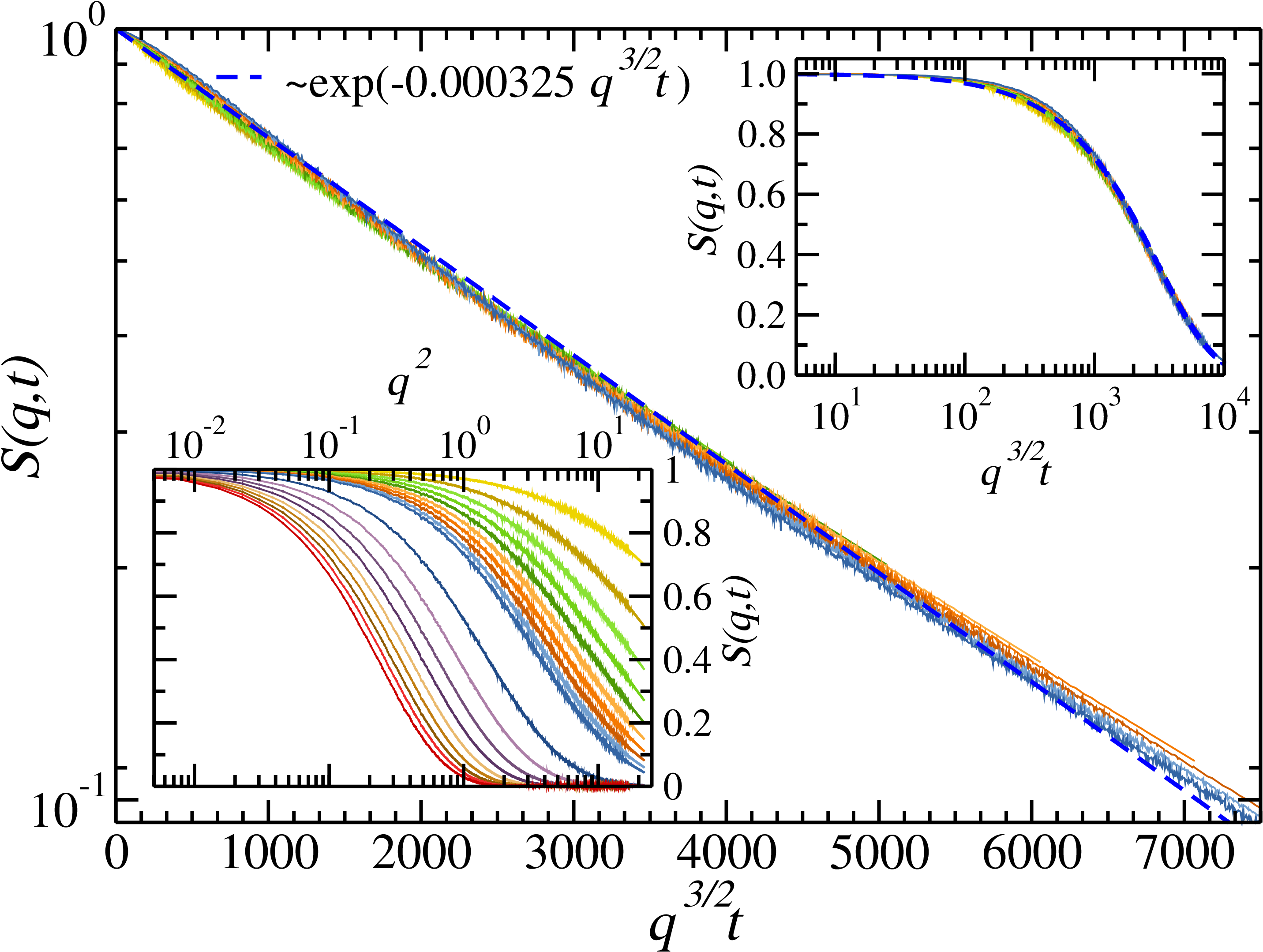
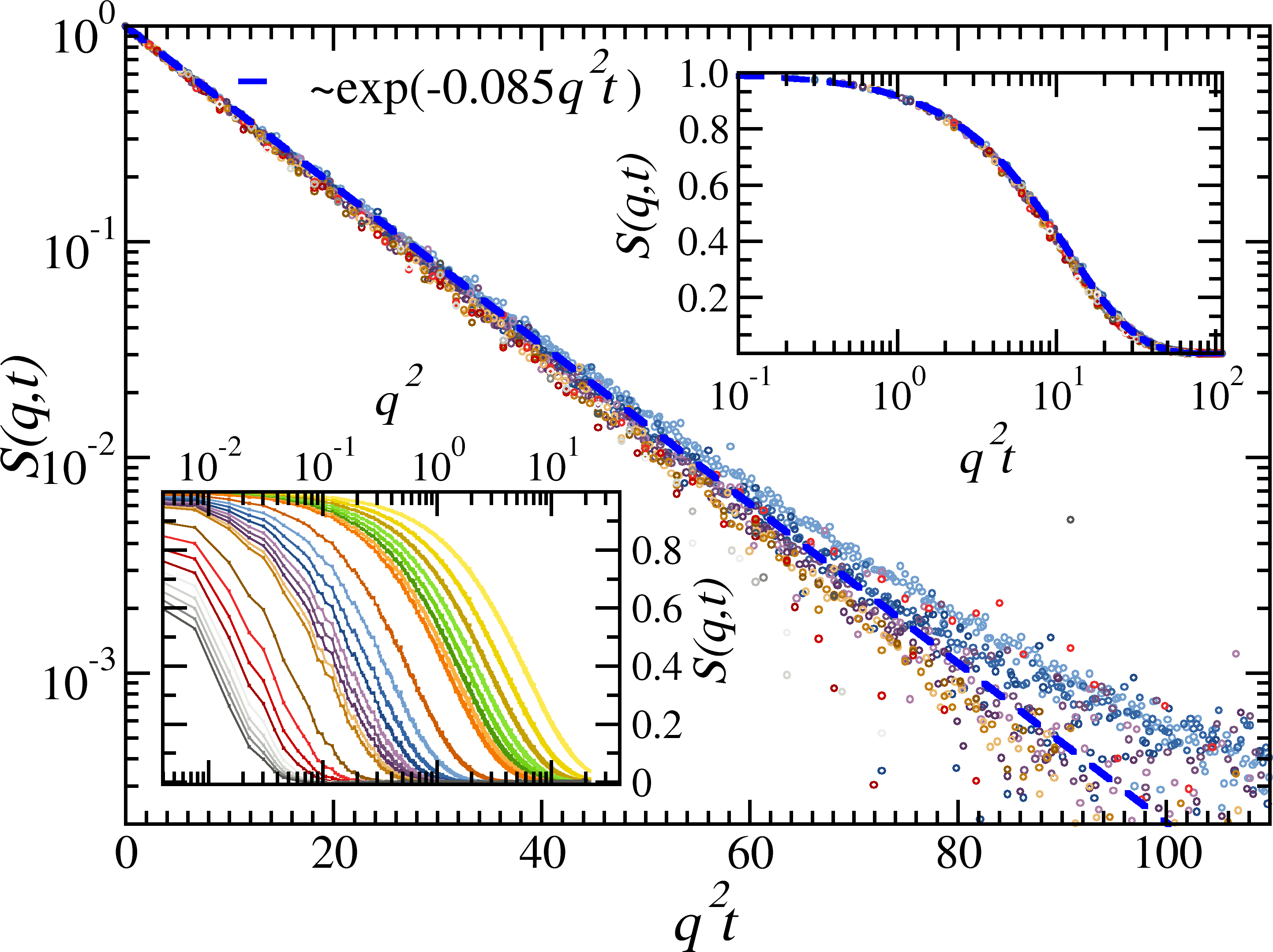
In Figure. 4 we show the dynamical structure factor for curves corresponding to long times ($t\gg\tau_{\tt ev}$). Without lack of generality, here we have used the data for $\tau_{\tt ev}=1.5$ to show comparatively much larger times. At observation windows $t\gg\tau_{\tt ev}$, we always expect to observe diffusion. Here, we see a collapse in the curves for times up to $t=1000$ when we plot $S(q,t)$ as a function of $q^{3/2}t$. The shape of the relaxation is now a simple exponential ($\beta=1$) $S(q,t)~{}\propto~{}\exp\left[-A\left(q^{3/2}t\right)\right]$. This is consistent with the mean-field prediction [16]: For $d=3$, $\tau_{r}\sim q^{-3/2}$ is expected for a diffusive process [16, 18] (see Eq.7 for the $\tau_{r}$ definition). Yet, at much longer times the $\tau_{r}\sim q^{-3/2}$ scaling breaks down. As explained by Bouchaud [18], $q^{3/2}$ reflects the fact that the ‘distribution of local displacements’ $P(u)$ has a diverging variance. For a distribution with a finite variance, one would recover the usual $q^{2}$ dependence in the exponential relaxation. As we show in the next section, $P(u)$ always has an upper cutoff. Therefore, it’s not surprising that dynamical structure factors measured over very long time windows already sense that finite variance and deviate from the $\tau_{r}\sim q^{-3/2}$ scaling. Moreover, the $u^{-5/2}$ tail is completely suppressed at higher plastic activities. This is a simple consequence of the central limit theorem. The response in the high activity regime is composed of a sum of a large number of random variables drawn from a distribution, which presents a cutoff at large displacements due to the finite core size of the plastic events. In this case, the $S(q,t)\sim\exp[-Aq^{3/2}t]$ regime completely shrinks to give place to a “purely diffusive” regime $S(q,t)\sim\exp[-Aq^{2}t]$, as the one observed in Brownian motion, already at time-windows 10 times larger than $\tau_{\tt ev}$. This is shown in Fig. 5, where we use $\tau_{\tt ev}=1.5$ and $T=0.16$ ($\left<a\simeq 0.15\right>$).

IV.1.3 Displacements distribution

As already mentioned, another quantity of interest is the characteristic displacement $u$ of a tracer particle in a given time window. More generally, we are interested in its distribution $P(u)$ at different temperatures.

In the limit of low temperatures (small plastic activities), we expect these displacements to be ruled by the fields generated by a few plastic events. We know that a plastic event induces a displacement $u\sim 1/r^{d-1}$, like a dipole. Close to a plastic event tracers will move a lot, large $u$, but statistically there will be more tracers further away from the event. More quantitatively, the probability of ‘seeing’ a plastic event at a distance between $\left[r,r+dr\right]$ when sitting on a random tracer will be proportional to $p(r)\sim r^{d-1}dr$ in general dimension $d$. Then, using probability conservation and $u\sim r^{-(d-1)}$ ($du\sim r^{-d}dr$)

$$P(u)du = P(r)dr$$

$$\propto r^{d-1}dr$$

$$\propto u^{-(2d-1)/(d-1)}du$$

Therefore, for large displacements we expect $P(u)$ to decay as $P(u)\sim u^{-(2d-1)/(d-1)}$, $P(u)\sim u^{-5/2}$ in $d=3$.

On the other hand, the statistics of small displacements will be ruled by an incoherent superposition of small ‘kicks’ given by distant plastic events. In a given finite system (and with periodic boundary conditions) one cannot be further than a maximum distance controlled by the density of events, from the closest plastic event. Then, it’s more frequent to find intermediate displacement values; since there are many more tracers at intermediate distances from the plastic events than far away. Indeed, one can prove that $P(u)$ should go to zero as $u$ decreases as $P(u)\sim u^{d-1}$. From just a pure incoherent Brownian motion and the resulting Maxwellian distribution for the displacements in a given time window, we are able to derive such $\sim u^{d-1}$ behavior at small $u$ for general $d$ (see Appendix. C).

Finally, in the limit of very low temperatures, the small displacements are not ruled by the incoherent superposition of many small kicks, but instead by the displacements field generated a very distant single (or few) plastic event(s). In this case we can expect $P(u)\!\sim\!u$ at small $u$.

Figure 6: Displacement distribution $P(u)$ for different temperatures. The tracers displacements absolute values $u$ are measured each $0.1$ time units. Panel (a) shows $P(u)$ for different temperatures $T=0.03,0.035,0.04,0.05,0.08,0.16$ and $0.27$ in different colors and symbols. The solid gray line correspond to the analytical expression of Eq. 21 for $c=0.016$. The inset of panel (b) shows the mean displacement $\left<u\right>$ vs mean activity $\left<a\right>$. The dashed line is a power-law $\sim\left<a\right>^{2/3}$. Panel (b) shows rescaled curves $P(u)\left<a\right>^{2/3}$ vs. $u/\left<a\right>^{2/3}$. Red dashed-line, purple dot-dashed-line and gray solid line show $P(u)\sim u$, $P(u)\sim u^{2}$ and $P(u)\sim u^{-5/2}$, respectively. $\tau_{\tt ev}=1.5$. $\epsilon_{0}=1.0$. $L=32$.

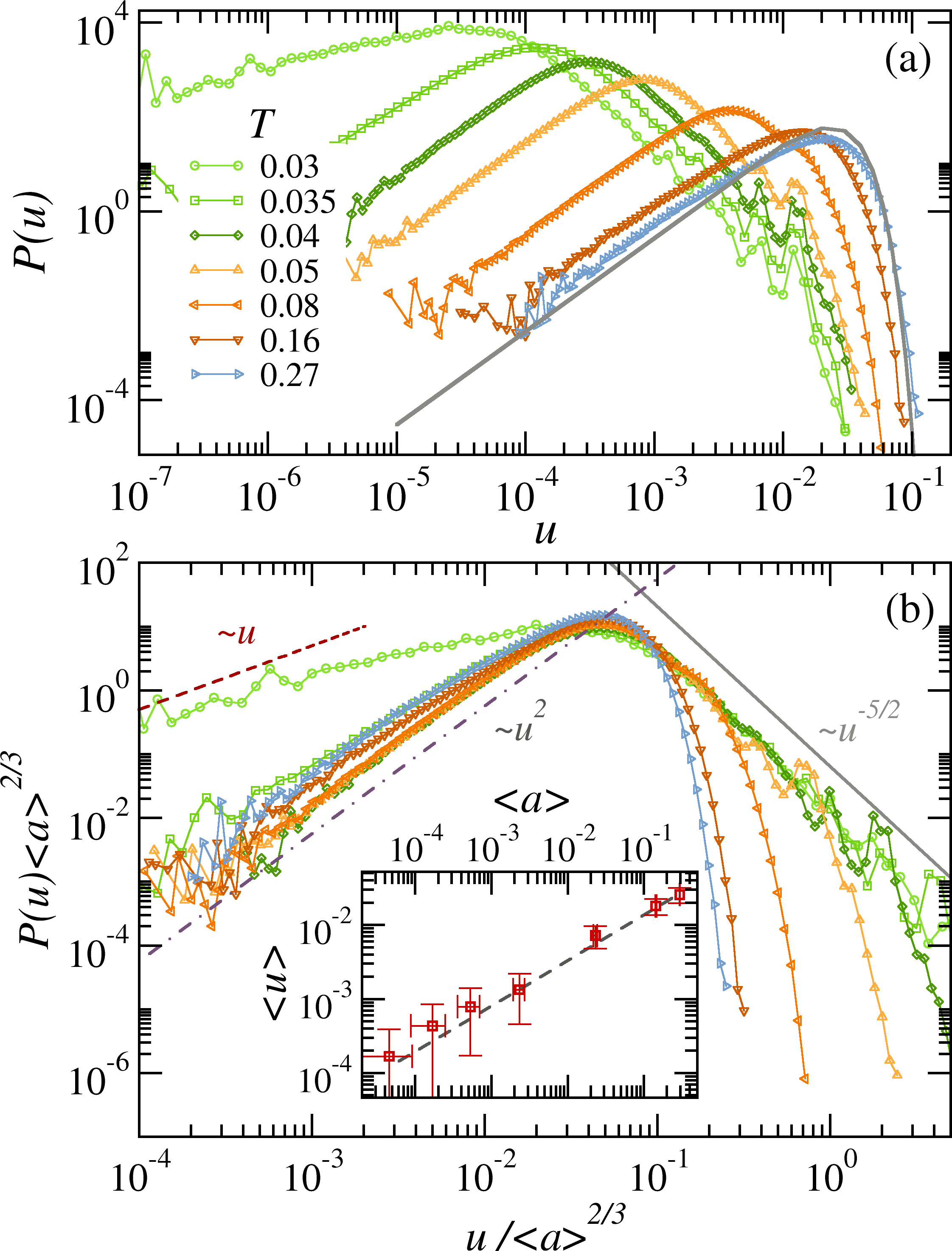
In Fig. 6(a) we show the displacement distribution $P(u)$, with $u$ defined as the absolute displacement in a time window $\Delta t=0.1$. These distributions have been obtained from $N_{d}\approx 1.1\times 10^{9}$ independent displacements of $M$ particles in the steady state. Let us first notice that the maximum of $P(u)$ moves to the right as the temperature increases. This is consistent with a larger average displacement value for tracers at larger and larger mean plastic activities. Which is something to be expected, since kicks coming from several neighboring events can add up to produce a larger displacement. We observe in particular that $\left<u\right>\propto\left<a\right>^{2/3}$ (Fig. 6(b) inset). The power-law cutoff at large $u$ is eventually controlled by the way the displacement field is computed on a lattice and the time integration of the displacement set up a natural maximum value. At each time step the displacement field cannot be higher than the one felt on a nearest-neighbor cell to an active plastic event. That kick times the $\Delta t$ of the displacement observation makes the maximum $u$, here $\sim 0.1$. Appendix C explores the dependence of $P(u)$ on $\Delta t$.

In Fig. 6(b) we use the $\left<u\right>\propto\left<a\right>^{2/3}$ scaling to ‘align’ curves corresponding to different temperatures. In this scaled plot, we can appreciate clearly the power-law decay of $P(u)$ for large displacements $\sim u^{-5/2}$; which extend to larger and larger ranges as temperature is lowered. The power-law behavior is disrupted at larger activities by the incoherent superposition of different plastic events effect on displacement fields. In fact, one can prove that for very high activities, where plastic events are basically uncorrelated, and induce an effective Brownian motion in tracer particles the distribution $P(u)$ takes the form of a Maxwellian (see gray line in Fig. 6(a)). The systematic little ‘peaks’ or oscillations observed in the distributions tails can be attributed to a discretization effect: integrating the tracer displacement over a field defined at patches makes some values of $u$ a priori more probable to obtain that others The choice of a larger time window to define $u$ washes out those oscillations (see App. C), so would do a smoothing of the displacement field (e.g., by interpolation).

IV.2 Fully thermal system

Up to now we have only considered tracer particles that follow displacement fields but that are themselves insensitive to temperature. We now turn to the slightly more realistic case in which we include thermal agitation in the tracer particles equations of motion. For each tracer $s$ we now update the tracer positions according to

$${\bm{\xi}}_{s}\to{\bm{\xi}}_{s}+\mathbf{u({\bm{\xi}}_{s})}dt+\eta_{s}(t,T)\sqrt{dt}$$ (20)

with $\mathbf{u({\bm{\xi}})}$ being the instantaneous displacement field at site ${\bm{\xi}}$, computed from the plastic activity (15) and $\eta_{i}(t,T)$ a Langevin thermal noise with zero mean value $\left<\eta_{i}(t,T)\right>_{t}=0$ and delta correlated $\left<\eta_{i}(t,T)\eta_{i^{\prime}}(t^{\prime},T)\right>=2T\delta(i-i^{\prime})\delta(t-t^{\prime})$. The motivation to include the last term in the tracers’ position updates comes from the fact that in thermal amorphous solids (metallic glasses and some colloidal glasses and gels [33, 46]) Brownian motion is relevant. It does not pretend to replace the complete atomistic modeling of interacting particles in a thermal bath, but add enough ingredients to sense the interplay of plasticity and temperature in a relaxing glass. Also, it turns into a closer model representation of the nanoparticles system presented in [6].

Note that this approach will only stand valid for small enough temperatures, such that the typical thermal displacements remain much smaller than the linear size of the thermally activated rearranging regions (cells of the EPM). Assuming such low temperatures is anyhow more opportune and realistic, since the compressed exponential relaxation is only expected in this regime [25]. With respect to Sec. IV.1 where only the ratio $B/(k_{B}T)$ was relevant (and $B=1$ was used), now the absolute value of $T$ also matters. In the following, we work with smaller values of $T$, but staying in a comparable range of $B/(k_{B}T)$ by decreasing $B$ accordingly.

In particular, we start by varying the temperature in the tracer’s e.o.m. while fixing the elasto-plastic model mean activity. This “fixed $\left<a\right>$ level” protocol would better mimic the cases in which plastic activity is considered to be largely controlled by rearrangements originated in pre-stress [25, 22]. To do that, we fix the ratio $B/(k_{B}T)$ in Eq. 13. For most of the Section we will set $\left<a\right>\simeq 0.05$, which, for comparison, correspond to a temperature $T\simeq 0.1$ when $B=1$, $\epsilon_{0}=1.0$ and $\tau_{\tt ev}$ = 1.5.

IV.2.1 Mean square displacement at fixed activity

Figure 7: Mean square displacement $\left<r^{2}\right>$ for a fixed plastic activity. The main plot shows the mean square displacement as a function of time observation window for different temperatures, ranging from $T=2.0\times 10^{-7}$ (light-green curve) to $T=6.3\times 10^{-4}$ (light-purple curve). The prefactor $B$ in Eq. 13 has been varied for each temperature such that $\left<a\right>(B/k_{B}T)\simeq 0.05$ is kept fixed. The gray full- and dashed-lines are guidelines to show the ballistic ($\sim t^{2}$) and diffusive ($\sim t$) behaviors, respectively. The inset shows a zoom-in to the short times regime ($t\leq\tau_{\tt ev}$). $\tau_{\tt ev}=20.0$. $\epsilon_{0}=0.1$. $L=32$, .

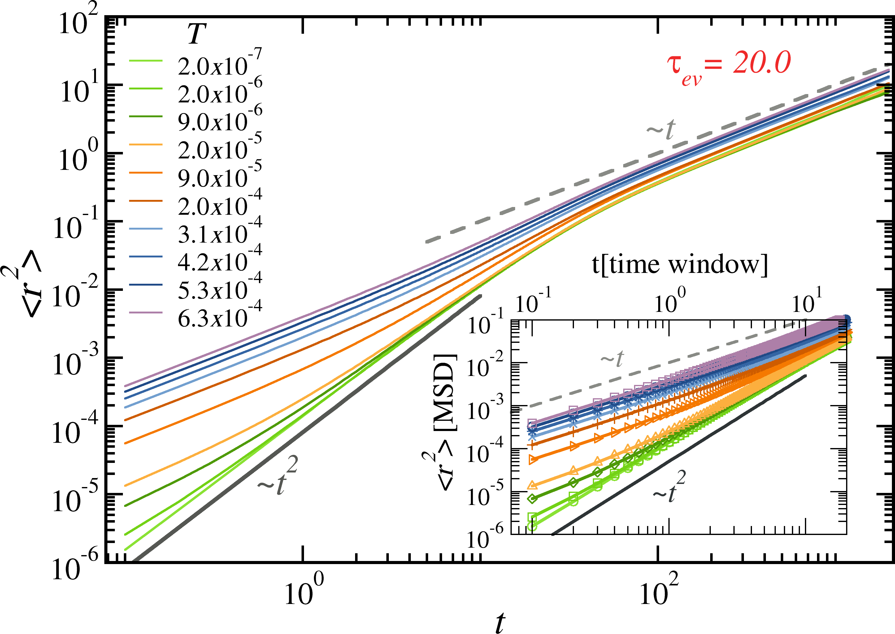
Figure 7 shows the mean square displacement of tracers at different temperatures and a fixed plastic activity at a low value $\left<a\right>\simeq 0.05$. At low temperatures, we observe the same crossover from a ballistic or persistent movement regime ($\left<r^{2}\right>\sim t^{2}$) to a diffusive regime ($\left<r^{2}\right>\sim t$) at $t\simeq\tau_{\tt ev}$ as reported in Fig.2. Notice that now we show the case of $\tau_{\tt ev}$ for a better display of the ‘short times’ ($t<\tau_{\tt ev}$) regime. As we increase the temperature, and thermal agitation becomes more and more relevant, we can observe how the ballistic regime is washed-out. While this is intuitive and somehow unsurprising, it hasn’t been addressed before (Ref. [19] worked only with athermal tracers and the mean-field approach of Pitard&Bouchaud didn’t include a thermal noise either). Explicitly modeling the interplay of plastic activity and temperature on tracer’s motion allows us to quantify the emergent dynamics. For example, one can notice that at intermediate temperatures in Fig. 7 the MSD shows an ”s” shape. Indeed the $\sim t^{2}$ behavior is killed starting from the shortest times and therefore fore some combinations of activity and temperature one gets for the dynamical regimes as a function of time window: diffusive, super-difussive or even ballistic, diffusive again. This would certainly have a consequence in the characterization of the relaxation, since the dynamical structure factor is expected to be affected accordingly.

IV.2.2 Dynamical structure factor at fixed activity

Figure 8: Dynamical structure factor $S(q,t)$ relaxation at short times and different temperatures but fixed activity. In all panels, the insets shows $S(q,t)$ as a function of $q^{2}$ for time windows up to $t=70$. The dark-red curve corresponds to duration of plastic events, $\tau_{\tt ev}=20$. $\epsilon_{0}=0.1$. $L=32$. (a) The mainplot collapses the curves corresponding to time-windows $t\leq\tau_{\tt ev}$ by plotting $S(q,t)$ as function of $q^{1.1}t$. The dashed line shows a compressed exponential of $(q^{1.1}t)$ with $\beta\simeq 1.58$. (b) The mainplot collapses the curves corresponding to time-windows $t\leq\tau_{\tt ev}$ by plotting $S(q,t)$ as function of $q^{1.3}t$. The dashed line shows a compressed exponential of $(q^{1.3}t)$ with $\beta\simeq 1.45$. (c) The mainplot collapses the curves corresponding to all time-windows by plotting $S(q,t)$ as function of $q^{1.7}t$. The dashed line shows a compressed exponential of $(q^{1.7}t)$ with $\beta\simeq 1.15$.

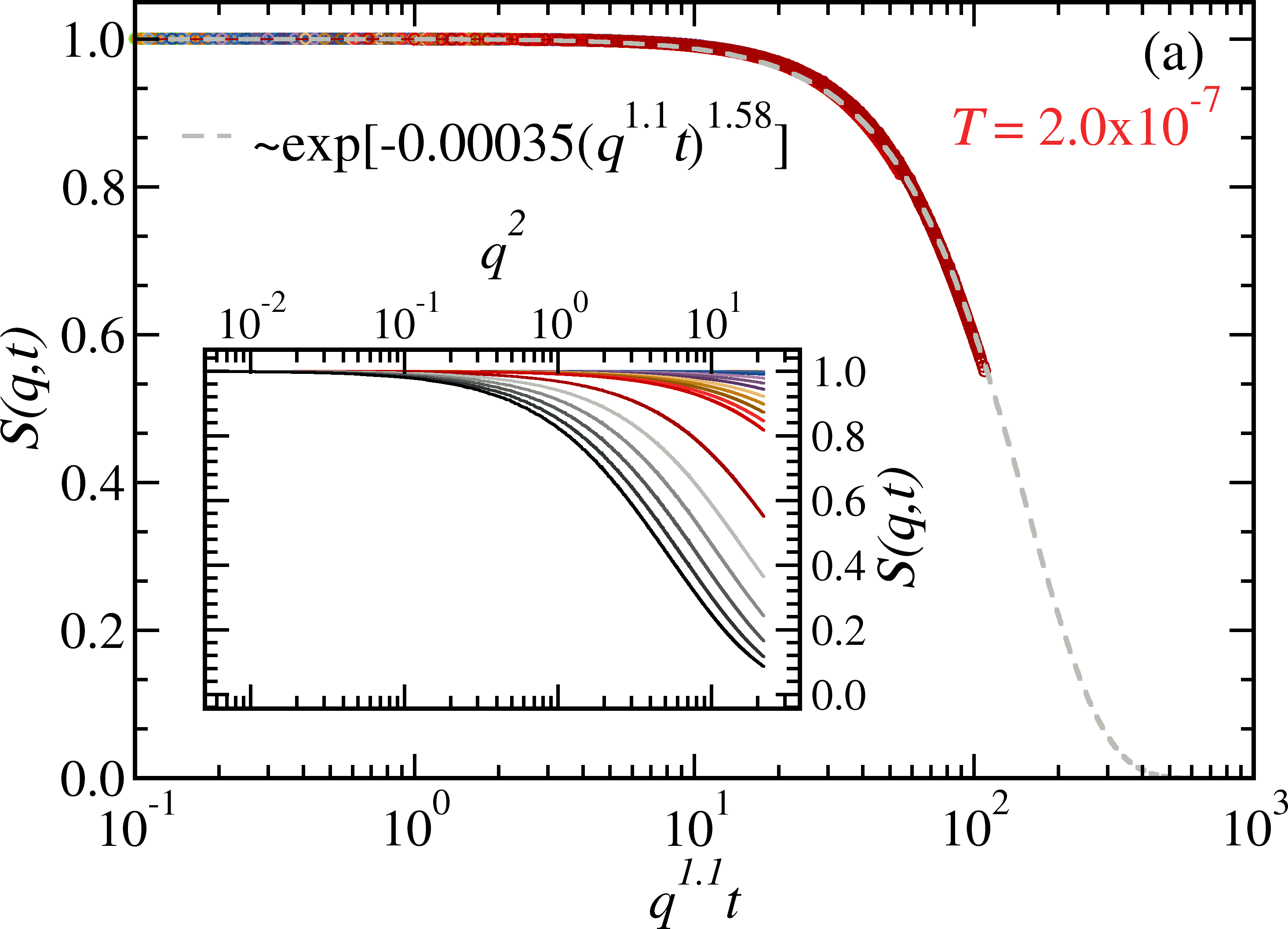
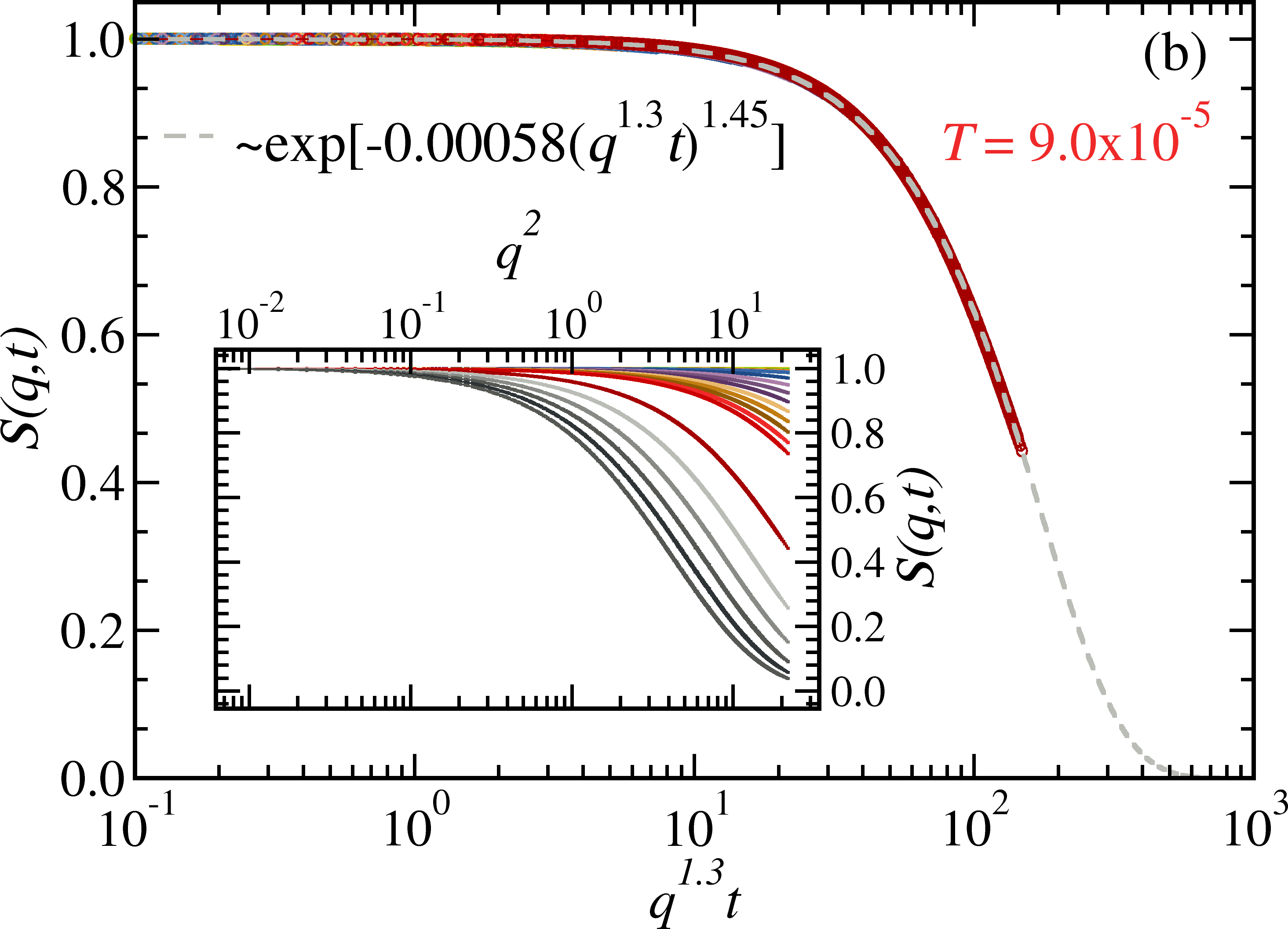
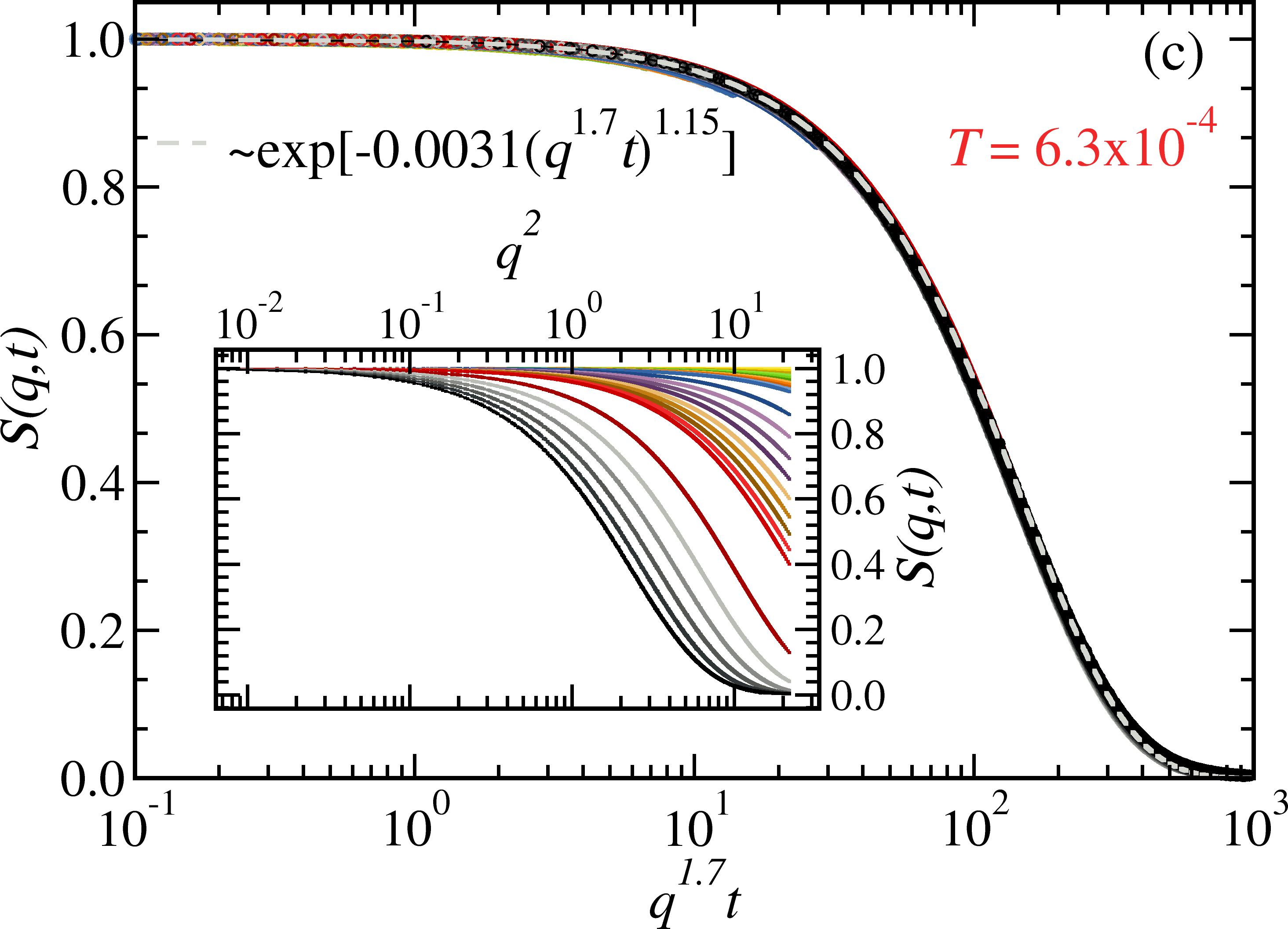
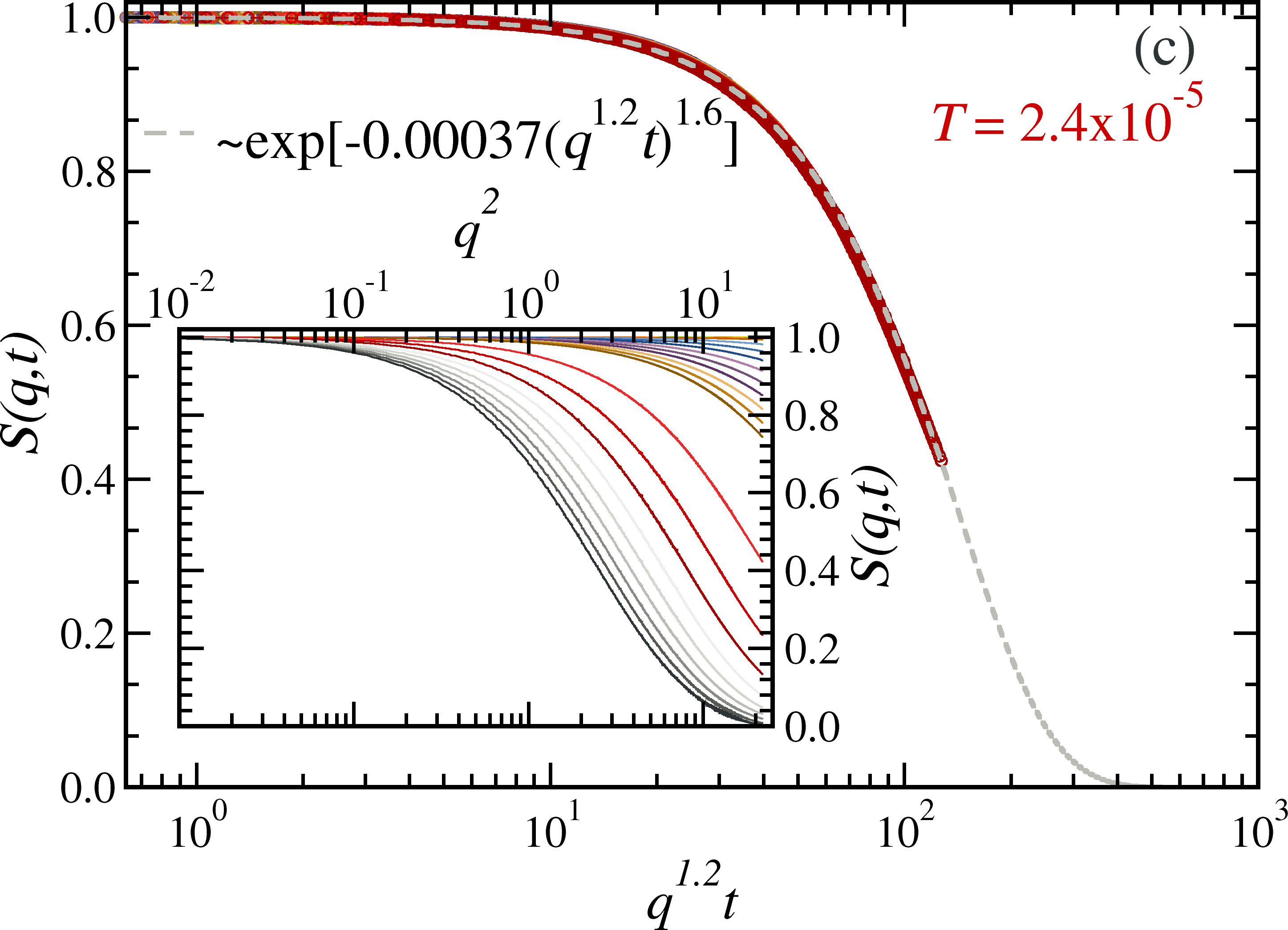
Thermal agitation on the particle tracers interferes in their persistent movement at short times and this has also consequences on $S(q,t)$. Figure 8 shows the dynamical structure factor $S(q,t)$ in the short-time regime for three different temperatures ($T=2.0\times 10^{-7}$, $9.0\times 10^{-5}$ and $6.3\times 10^{-4}$) at fixed activity, i.e., corresponding to the two extremes and an intermediate curve of Fig. 7. In the raw data of the insets one can appreciate that for a given time-window (same curve color in the three panels) and same $q$, $S(q,t)$ has relaxed more at higher temperatures. This is intuitive since thermal agitation contributes to the decorrelation from the initial configuration. Nevertheless, the interesting characteristics lies in the functional form of the relaxation. For each temperature we seek for structure factor behavior of the form $S(q,t)\propto\exp\left[-A(q^{\alpha}t)^{\beta}\right]$. In panels (a) and (b) we have collapsed curves corresponding to time-windows up to the duration of the plastic event ($t\lesssim\tau_{\tt ev}$), while in (c) the good collapse with a single $\alpha$ extends to times above $\tau_{\tt ev}$. We observe that both $\alpha$ and $\beta$ varies with temperature. The results for the lower temperature here (panel (a)) are consistent with the athermal case presented in Fig. 3. As temperature increases, $\alpha$ increases from $\sim 1.1$ to $\sim 1.7$ while $\beta$ decreases from $\sim 1.58$ to $\sim 1.15$.

This goes in the direction of a crossover between a persistent movement regime and a diffusive regime, as postulated in Fig. 7. Indeed, if we take the mean-field exponents [18] as a guide, we may expect $\{\alpha,\beta\}$ moving from $\{1,3/2\}$ to $\{2,1\}$ as the temperature increases and the tracers at short times go from ballistic to diffusive. Yet, all exponents estimated from data are effective and not exactly matching the mean-field ones. One can argue that this is caused on one hand due to the crossover between dynamical regimes at $t\sim\tau_{\tt ev}$ itself, but more importantly, due to the fact that the system is in finite dimensions and non-trivial correlations among plastic events are expected to play a role.

Figure 9: Relaxation exponent $\alpha$ and $\beta$ at short times for different temperatures but fixed activity. The upper-panel shows $\alpha$ vs. $1/T$ and the lower-panel displays $\beta$ vs. $1/T$. The $1/T$ axis is displayed in log-scale simply for a better visualization. The estimates correspond to collapses and fits as those of Fig. 8. $\tau_{\tt ev}$ = 20.0. $\epsilon_{0}$ = 0.1. $L=32$.

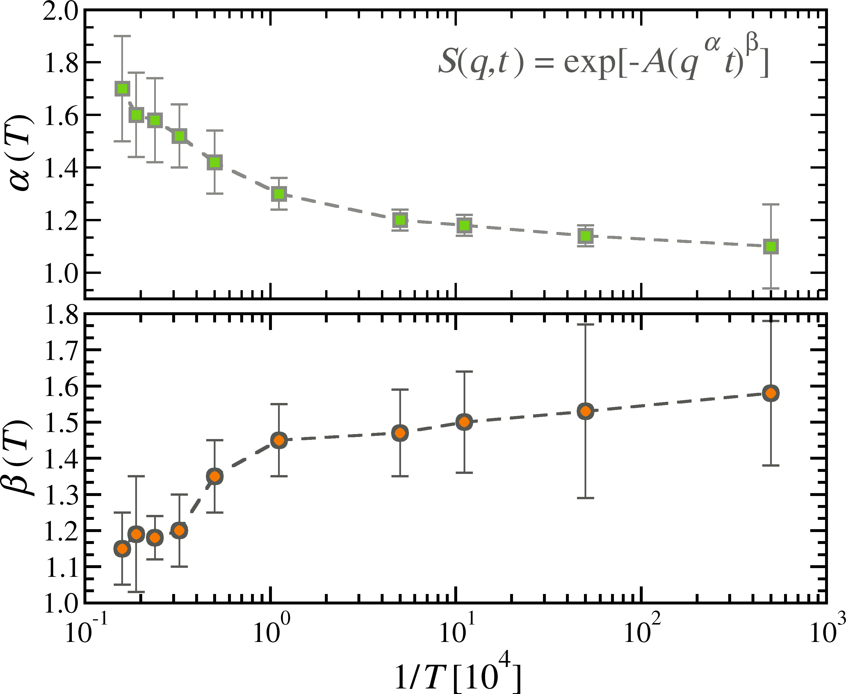
Figure 9 shows the evolution of $\alpha$ and $\beta$ with temperature. The exponents have been measured for several temperatures from collapses and fits as the ones in Fig. 8. The error bars are estimated from independent fit approaches and then doubled. Let us notice first in the bottom panel how $\beta$ increases from $\sim 1.1$ to $\sim 1.6$ as the temperature is lowered. These results can be compared with the recent reports in Zr_46.8Ti_8.2Cu_7.5Ni₁₀Be_27.5 metallic glass ($T_{g}\simeq 596K$) presented in Ref. [21], where $\beta$ decreases with increasing temperature smoothly from $1.75\pm 0.14$ at 523 K to $0.67\pm 0.07$ at 618 K. A stretched exponent $\beta<1$ indicates that the sample has reached the super-cooled liquid state (inaccessible in our model). Earlier [32], the shape factor $\beta$ was studied for Mg₆₅Cu₂₅Y₁₀ ($T_{g}\simeq 405K$), showing that it remained in the range 1.7-1.4 before plunging when approaching $T_{g}$. Our results for the temperature dependence of $\beta$ are also consistent with what has been reported in simulations of network-forming gels [25]. Accompanying the gradual change of $\beta$ with temperature, the exponent $\alpha$, that defines how the characteristic relaxation time depends on the wave vector, decreases with decreasing temperature, from $\sim 1.7$ (diffusive-like) to $\sim 1.1$ (ballistic-like). In other words, for a fixed $q$ the characteristic relaxation time $\tau\sim q^{-\alpha}$ decreases with increasing temperature. Again, in agreement with [32, 25, 21].

We therefore propose that the shape exponent variation with temperature in measured relaxation of amorphous solids can be understood by the competition of rather persistent displacements on its essential constituents, induced by the occurrence of plastic events nearby, on one hand, and the intrinsic thermal agitation at which they are subject that tends to generate a Browninan motion of particles.

IV.2.3 Displacements distributions with thermal agitation

Figure 10: Displacement distribution $P(u)$ for different mean activities with and without thermal agitation (TA). Green curves relate to an activity $\left<a\right>\simeq 0.00017$: while open symbols repeat the data for $T=0.035$ in Fig. 6, closed symbols correspond to $T\simeq 8\times 10^{-7}$ ($B$ changes to maintain activity) an thermal agitation proportional to $T$ has been included in the tracers. Orange curves relate to $\left<a\right>\simeq 0.0023$ ($T=0.05$ in Fig. 6), and the thermal agitation included in this case is $T\simeq 8\times 10^{-5}$. Red dashed-line, gray dashed-point line show $P(u)\sim u^{2}$ and $P(u)\sim u^{-5/2}$, respectively. The tracers displacements absolute values $u$ are measured each $0.1$ time units. $\tau_{\tt ev}=1.5$. $\epsilon_{0}=1.0$. $L=32$.

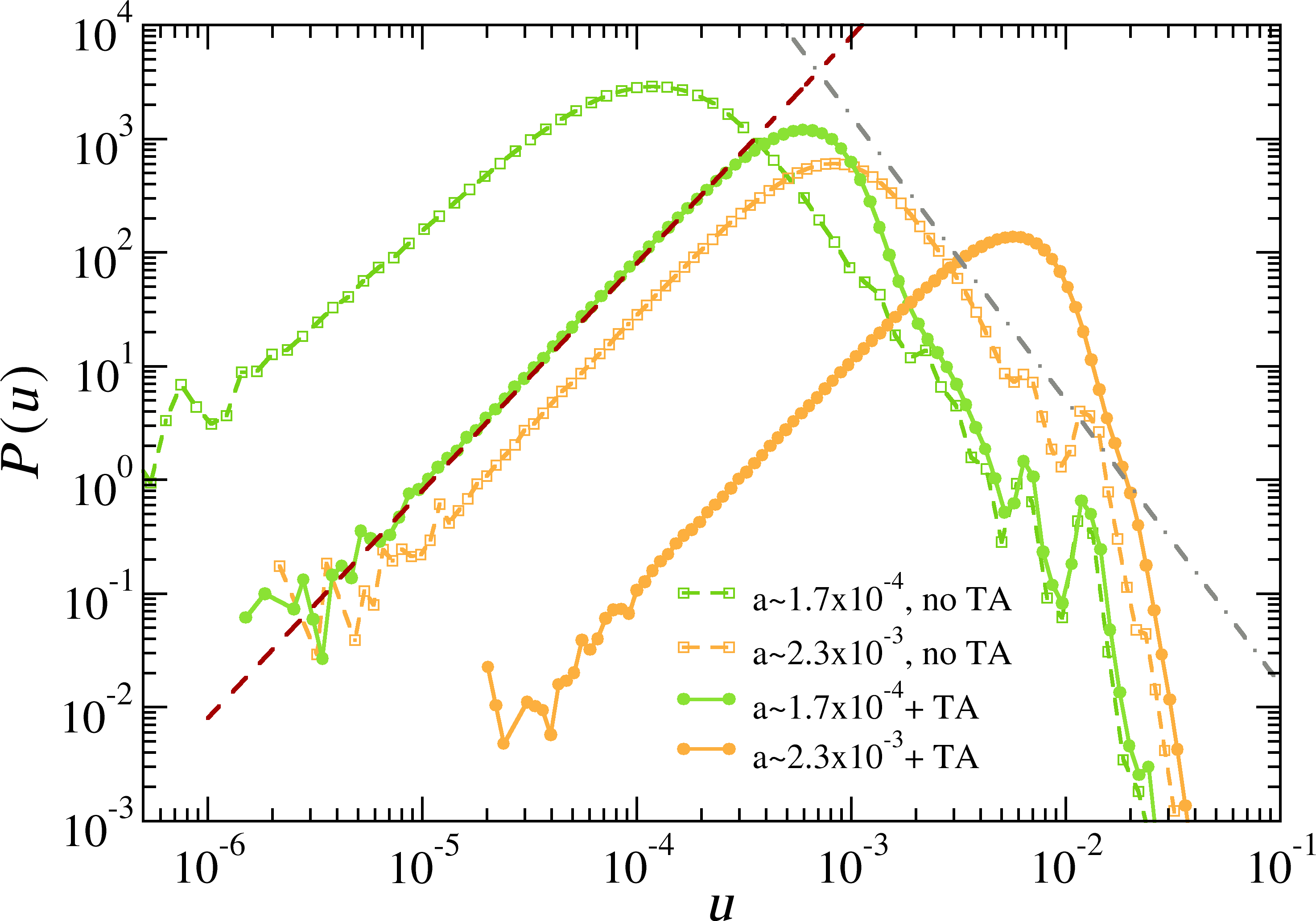
To complete the picture of what happens when we include thermal agitation in the tracer particles, we present here the displacement distributions $P(u)$ for a couple of temperatures with the addition of thermal agitation on the tracer movement. Figure10 shows $P(u)$ for a couple of different temperatures to see the thermal agitation effect on the displacements. Green solid points correspond to a relatively low temperature of $T\simeq 8\times 10^{-7}$ (and $B=2.3\times 10^{-5}$ is equally low such that $\left<a\right>\simeq 0.00017$) We can see that, although the large $u$ tail of P(u) is still dominated by the plastic activity induced displacements, the thermal agitation or Brownian motion of the tracers start to dominate the small displacements, clearly shifting the $P(u)$ peak position (comparison is done with the {$T=0.035$, $B=1$} curve of Fig. 6). For the orange solid points $T\simeq 8\times 10^{-5}$ is already large enough to completely erase the hallmark of the displacements of mechanical origin (comparison is done with the {$T=0.05$, $B=1$} curve of Fig. 6). The $P(u)\sim u^{-5/2}$ behavior at large $u$ completely disappears, while the $P(u)\sim u^{2}$ scaling at small $u$ still shows, but now directly generated by a genuine Brownian motion instead of being a result of an incoherent superposition of displacements with mechanical origin (see App.C). The disappearance of the $P(u)\sim u^{-5/2}$ tail at large enough temperatures, justifies a diffusive regime $S(q,t)\sim\exp[-Aq^{2}t]$ stepping in sooner than in the pure plastic activity case, as we verify.

IV.3 Reactivation-times and dynamical heterogeneity

Figure 11: Distribution of reactivation times $\Psi(\tau_{\tt re})$ for different temperatures. $\tau_{\tt re}$ are the time lapses between consecutive occurrences of a plastic event in the same system patch. Upper-panel shows raw data for different temperatures (activity levels). Red-dashed line displays a power-law $\sim\tau_{\tt re}^{-\omega}$, with the exponent $\omega=3/4$. Lower-panel rescales the curves plotting $\Psi(\tau_{\tt re})/\left<a\right>^{1.07}$ vs $\tau_{\tt re}\left<a\right>^{1.07}$. $B=1.0$. $\tau_{\tt ev}$ = 1.5. $\epsilon_{0}$ = 1.0. $L=32$,

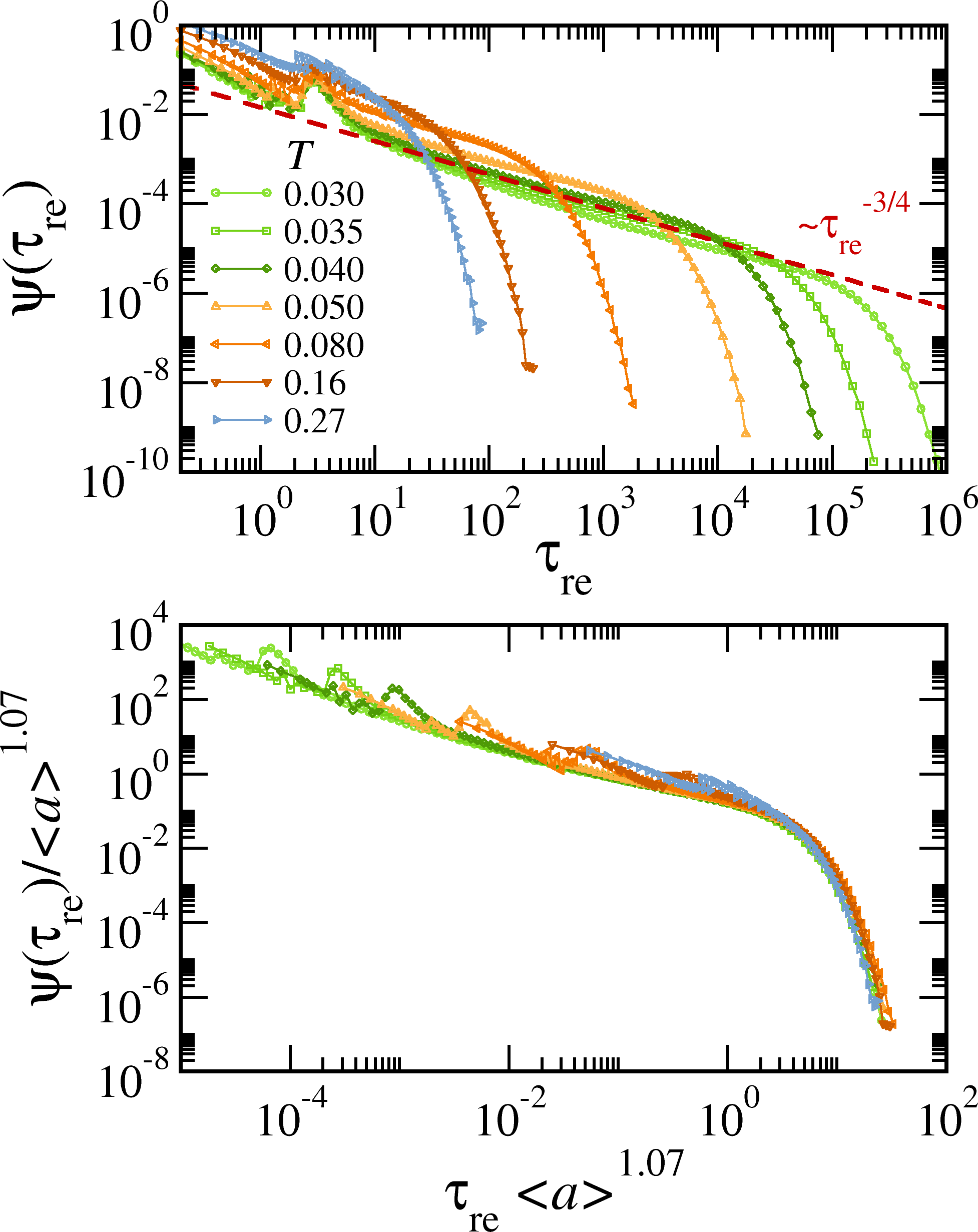
So far we have concentrated in quantities that are computed from the tracer particle movements. We now focus on the evolution of the elasto-plastic system itself and jump to the analysis of the intermittent and heterogeneous dynamics observed in the quiescent amorphous solid. System patches locally yield, either activated by temperature or over-stressed by the action of other sites; then they recover elasticity (on average) after a time $\tau_{\tt ev}$. The time takes to see two consecutive activations of a given site will depend somehow trivially on the global activity level, but each occurence can be difficult to predict. In fact, this quantity -that we call “reactivation-time” $\tau_{\tt re}$- is broadly distributed, in particular at low temperatures.

In Fig.11 we show $\Psi(\tau_{\tt re})$ for different temperatures. Beyond short $\tau_{\tt re}$, one sees a power-law distribution $\Psi(\tau_{\tt re})\sim\tau_{\tt re}^{-\omega}$, with $\omega\simeq 3/4$, followed by an exponential upper cutoff. Interestingly, the cutoff depends on temperature and moves to larger and larger reactivation times as $T$ is decreased. For our lowest temperatures, $\Psi(\tau_{\tt re})$ expands over almost 7 orders of magnitude. As expected, $\tau_{\tt re}$ seems be proportional to an activation rate that scales as the inverse of activity $\left<a\right>^{-1}$, and we can use that to collapse the distribution tails in Fig.11(bottom). We find that an exponent close but not exactly unity makes the best collapse, happening when we plot $\Psi(\tau_{\tt re})/\left<a\right>^{1.07}$ vs $\tau_{\tt re}\left<a\right>^{1.07}$, preserving the normalization of the distributions rather than the power-law exponent. As already discussed in [19], the interaction among plastic events cause the emergence of a characteristic short reactivation time of the order of $\tau_{\tt ev}$, presumably due to neighbor sites alternately triggering each other during a burst of activity. That is the little peak observed in all curves, that looks sharper at low temperatures. At the same time, correlations among sites induce a fat-tailed distribution of reactivation times, that are increasing as $T$ decreases, which otherwise would decay exponentially in a Poissonian way. At low temperatures, the intermittency of the plastic events at a given site is determined by events happening in other regions of the system, it’s intrinsically a spatial property. Furthermore, notice that the exponent $\omega$ controlling the power-law regime depends on dimension: It was $\omega\simeq 2/3$ in $d=2$ and it’s now $\omega\simeq 3/4$ in $d=3$. Although one can be tempted to think on a $d/(d+1)$ dependence, we don’t have an argument for this observation. Intermittency was argued as a possible explanation of the shape exponent $q$-dependence [5]. While we don’t address that problem in the present work, it’s worth mentioning that in EP models the activation times of a block is a direct observable. So this is advantageous for studies of intermittency of plastic activity.

Figure 12: Distribution of mean reactivation times $\Psi(\left<\tau_{\tt re}\right>)$ for different temperatures. $\left<\tau_{\tt re}\right>$ are the average time lapses between consecutive occurrences of a plastic event in each block of the system. Averages are taken over 10² local measurements of $\tau_{\tt re}$ very well separated in time (non-correlated), and the histogram is computed with the statistics of $2^{15}$ blocks. $B=1.0$. $\tau_{\tt ev}$ = 1.5. $\epsilon_{0}$ = 1.0. $L=32$.

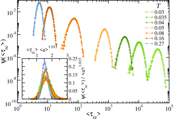
One is tempted to relate this broad distribution of reactivation times to dynamical heterogeneities. In fact, dynamical heterogeneities have been recently discussed in thermal EPMs. In [37], it is argued that the patterns formed by the local persistence at different temperatures show that the dynamics is spatially heterogeneous over lengths that increase when lowering the temperature. Nevertheless, at least in our case, it can be seen clearly that such heterogeneity in space is only momentary and do not persist when the dynamics is integrated in time. In other words, one does not find the paradigmatic dynamical heterogeneity of glasses where for example, as in spin glasses, persisting fast and slow regions can be identified [52, 53, 54]. In the absence of anisotropic fields or disorder in the local activation dynamics, such as a quenched disorder or a dynamical disorder creating diverging correlation times, the system is intrinsically homogeneous and we observe such homogeneity in the time averages of $\tau_{\tt re}$. In Fig. 12 we take the average reactivation time on each block during a long run, with care to average over uncorrelated samples, this is, taking well separated configurations in time, and we plot its distribution using our $2^{15}$ blocks as a representative statistics. It is interesting to see that the mean value $\left<\tau_{\tt re}\right>$ is well peaked around a typical value that depends on temperature (activity). The moving peak/bump at large $\left<\tau_{\tt re}\right>$ is simply a signature of blocks needing to wait more and more to get re-activated as $T$ decreases.

V Discussion

We have used a three-dimensional thermal elasto-plastic model with the addition of probe particles to follow the displacement fields and analyze the equilibrium structural relaxation dynamics of quiescent amorphous materials at finite temperatures. The results show that for sufficiently short times and when the plastic activity is relevant, there is always a super-diffusive regime in the mean square displacement of the probe particles, after which they enter a crossover towards a diffusive behavior. The crossover is dominated by the typical duration of plastic events in agreement with the interpretation that the close to linear motion of the particles in the super-diffusive part is an elasticity-mediated phenomenon.

In addition, we observed a compressed exponential relaxation (with a shape exponent $\beta$ reminiscent of experimental results) in the dynamical structure factor $S(q,t)$ at short times, associated with the elasticity-mediated super-diffusive regime, that exists even in the equilibrium dynamics of this model. For a sustained plastic activity level, the $\beta\!>\!1$ exponent varies with temperature, decreasing as the thermal agitation of the particles becomes more and more relevant, eventually turning the compressed- into a simple-exponential ($\beta\sim 1$).

At long times, in the diffusive regime, the relaxation is always exponential. Furthermore, we observe the crossover from a $(q^{3/2}t)$ to a $(q^{2}t)$ diffusive relaxation when activity increases, as predicted by mean-field arguments [16, 17]. The displacements distribution $P(u)$ helps to interpret the behavior of $S(q,t)$, with the characteristic $P(u)\sim u^{-5/2}$ decay of large displacements (also expected from mean-field arguments) disappearing as the mean activity increases.

We noticed that our approach does not reproduce in any regime the characteristic stretched exponential relaxation of glasses . Reproducing the commonly observed stretched exponential relaxations at long times seems not possible without further complexification of the EP model under consideration. A common belief is that stretched exponentials are created by the superposition of a large distribution of relaxation times in the glassy heterogeneous dynamics [56]. In our thermal elasto-plastic model, we show indeed a feature of dynamical heterogeneity (similar to [37]): a very wide distribution of activation ‘waiting’ times is observed instantaneously. Yet, the system remains homogeneous in the time-integrated dynamics, and stretched relaxation never happens. Without a quenched disorder or other kind of imposed persistent heterogeneity, we don’t believe that stretched exponentials can be reproduced in elasto-plastic models.

Still, other avenues to explore modifications of elasto-plastic models towards the characterization of glasses are possible. Recent studies have shown that stretched exponential behavior in glasses could be observed already on a local scale relevant to the localized relaxation events [57], and stretched exponentials can thus be obtained independently of a broad distribution of relaxation times. Also, stretched exponential relaxation can be obtained by appropriately tweaking the dynamics of local relaxation events and weighting their interactions, at least in a mean-field approach [27]. We can envision that modifications on how local stress relaxation occurs in plastic events in elasto-plastic models, e.g. abandoning the simplistic instantaneous, simple exponential or linear options explored so far, might also allow for a stretched relaxation regime to arise in the dynamics, irrespective of the system homogeneity. Furthermore, EP models could also serve as a numerical tool to compare with recent under-pressure relaxation measurements in BMGs [58], through an easy modification of the model implementation and parameters.

Finally, we expect that our analysis of the interplay between plastic activity induced displacements and simple agitation due to finite temperature would inspire ongoing experiments on systems whose elementary constituents and are sensitive to Brownian motion to try to discriminate both contributions in the auto-correlation functions of the scattered intensity; for example, by independently assessing the ‘mean plastic activity’ during the experiment as temperature is varied.

Appendix A Steady-state stress distribution

This Appendix shows the stationary distribution of stresses in our elasto-plastic model at different temperatures or activities. In the way the model is defined, it only makes physical sense if the plastic activity is “low enough”. High activity levels, induce a notable fraction of the blocks to remain over-stressed and “out of the box” $\left[-\sigma_{y},\sigma_{y}\right]$. That is to be avoided if we want to make sense of the results. Therefore, our control observable has been the distribution of stress at each given temperature or mean activity.

Figure 13: Stress distribution for different temperatures in the stationary state. Parameters: $B=1$ and $T$ ranging from $0.03$ to $0.27$ as indicated in the legends, with respective mean activities $\left<a\right>\simeq 4.5\times 10^{-5}$, $1.7\times 10^{-4}$, $5\times 10^{-4}$, $2.3\times 10^{-3}$, $0.023$, $0.14$, $0.3$. $\tau_{\tt ev}$ = 1.5. $\epsilon_{0}=$ 1.0. $L=32$.

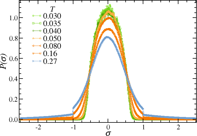
Figure  13 shows the normalized stress histograms $P(\sigma)$ corresponding to the steady states used to produce Fig. 2. As plastic activity increases, the stress distributions become wider and wider. The local yield stresses, being set to $\sigma_{y}=\pm 1$, make the distribution to show a pseudo discontinuity as the stress $\sigma$ goes out of the box. Let us recall than for these steady states, the prefactor of the Arrhenius term was simply $B=1$ and $T=0.03,...,0.27$ induced mean activities of $\left<a\right>\simeq 4.5\times 10^{-5},...,0.3$.

Figure 14: Stress distribution for different temperatures in the stationary state. Parameters $B$ and $T$ as shown in the legends, preserving a mean activity $\left<a\right>\simeq 0.05$. $\tau_{\tt ev}$ = 20, $\epsilon_{0}$ = 0.1. $L=32$.

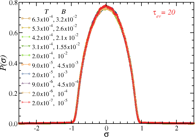
Moving to the analysis of the interplay between plastic activity and thermal agitation we have fixed a plastic activity to $\left<a\right>\simeq 0.05$ varying accordingly $B$ and $T$. Figure 7 shows the distributions $P(\sigma)$ for the steady states of such cases. As one expects, the stress distribution only depends on the mean activity and all curves coincide.

Appendix B Mean plastic activity $\left<a\right>$ vs temperature

The mean plastic activity $\left<a\right>$ is directly controlled by the temperature $T$ and the parameter $B$ through Eq. 13, but it also depends on the effect that a plastic event has on other sites, which is modulated by $\epsilon_{0}$, and in the plastic events duration $\tau_{\tt ev}$. In this Appendix, we show activity as a function of temperature for the case corresponding to the steady states of {$B=1$, $\tau_{\tt ev}=1.5$, $\epsilon_{0}=1.0$} and {$B=0.001$, $\tau_{\tt ev}=20$, $\epsilon_{0}=0.1$}.

Figure 15: Main plots: Mean plastic activity $\left<a\right>$ vs $1/T$ in the stationary state Insets: $\left<a\right>$ vs $T$. Upper panel: $B=1$, $\tau_{\tt ev}=1.5$, $\epsilon_{0}=1.0$ and $L=32$. Lower panel: $B=0.001$, $\tau_{\tt ev}=20.0$, $\epsilon_{0}=0.1$ and $L=32$.

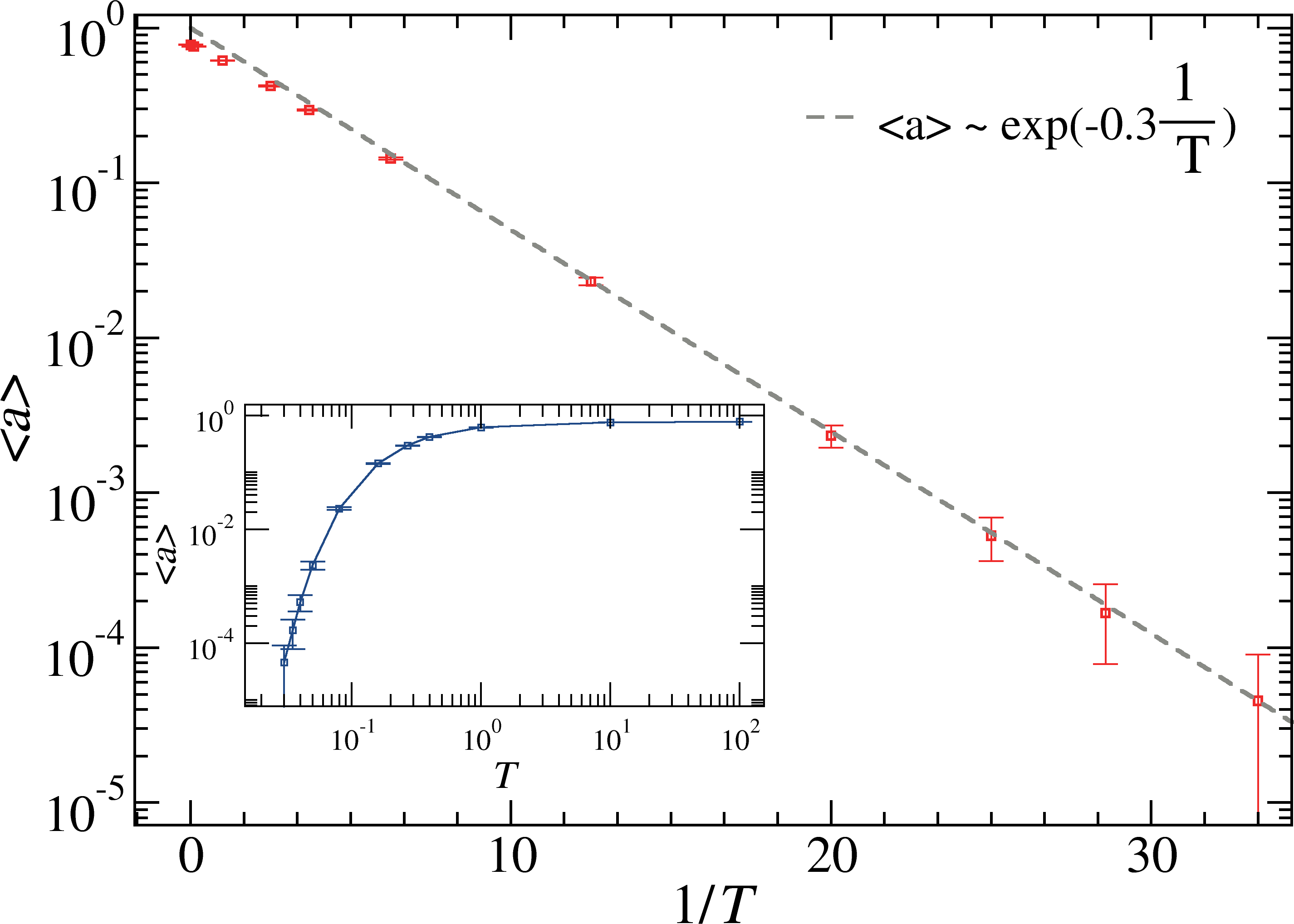
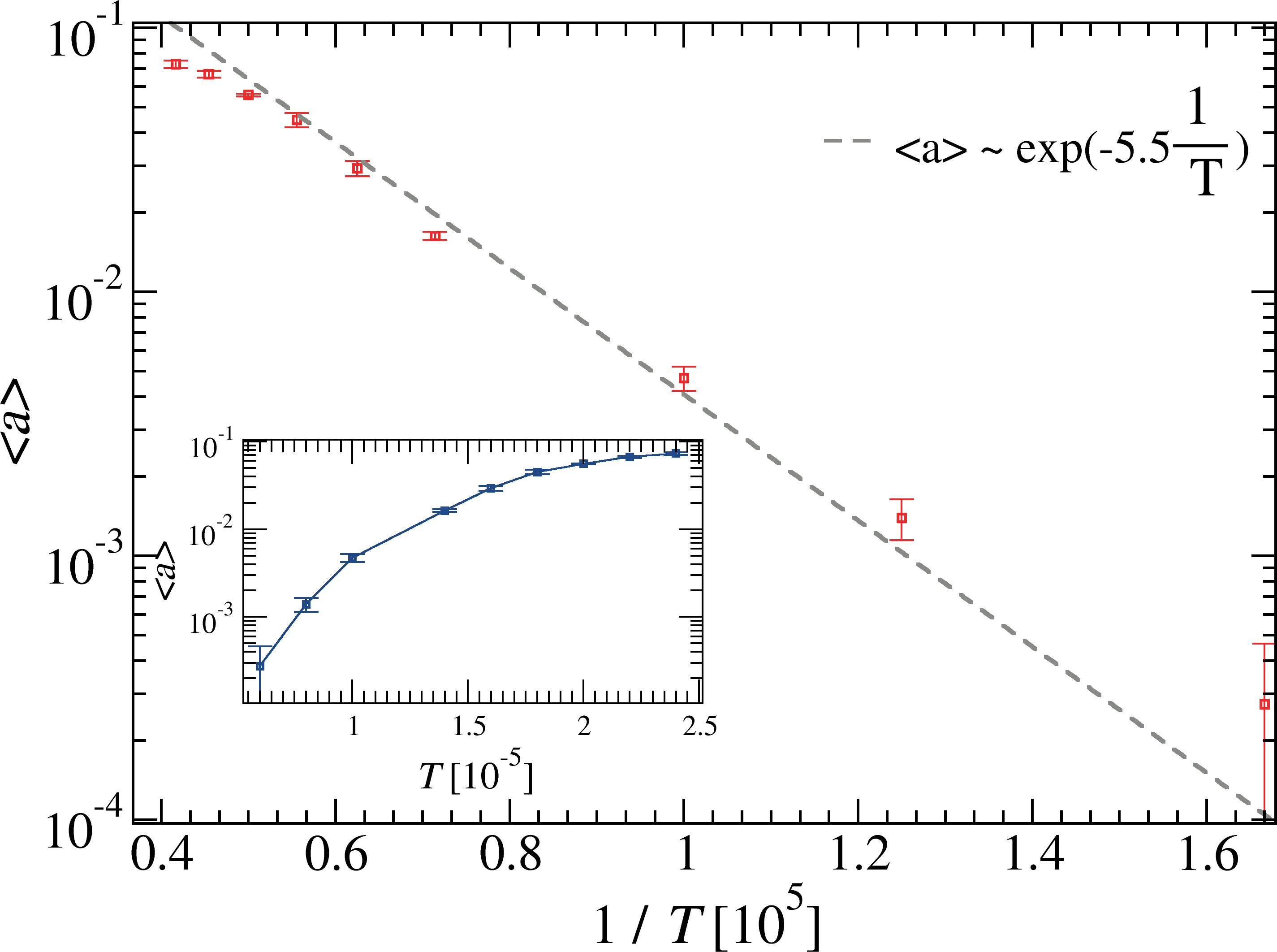
Figure 15 upper panel shows the mean activity $\left<a\right>$ as a function of $1/T$ for the same steady states as in Fig. 2 (plus some extra temperatures). The behavior of the activity is exponential in $1/T$, as expected. The inset, plotted in log-lin, shows $\left<a\right>$ vs $T$. We can appreciate that for $T\to 0$ the activity decays fast, while, on the other hand, it saturates at large temperatures. The lower panel shows $\left<a\right>$ vs. $1/T$ (main panel) and $T$ (inset) for the same steady states as in Fig. 18.

Appendix C Displacement distribution $P(u)$: different acquiring time and Brownian motion role

This Appendix intends to help in the interpretation of the results for the displacements distribution $P(u)$. On one hand, the definition of $u$ itself depends on a time window observation. $u$ is defined as the displacement of a tracer in a given time $\Delta t$. Changing $\Delta t$, changes $u$ and therefore also $P(u)$. On the other hand, it’s important to understand the limit cases.

Displacement distribution for different definitions of $u$.

Figure 16: Displacement distribution $P(u)$ where $u$ is defined as a tracers displacement time window $\Delta t$ (different values of $\Delta t$ indicated in the legends). Parameters: $T=0.03$, $\tau_{\tt ev}=1.5$, $\epsilon_{0}=1.0$, $L=32$. Red-dashed, gray point-dashed and gray full-line show $P(u)\sim u$, $\sim u^{2}$ and $\sim u^{-5/2}$, respectively.

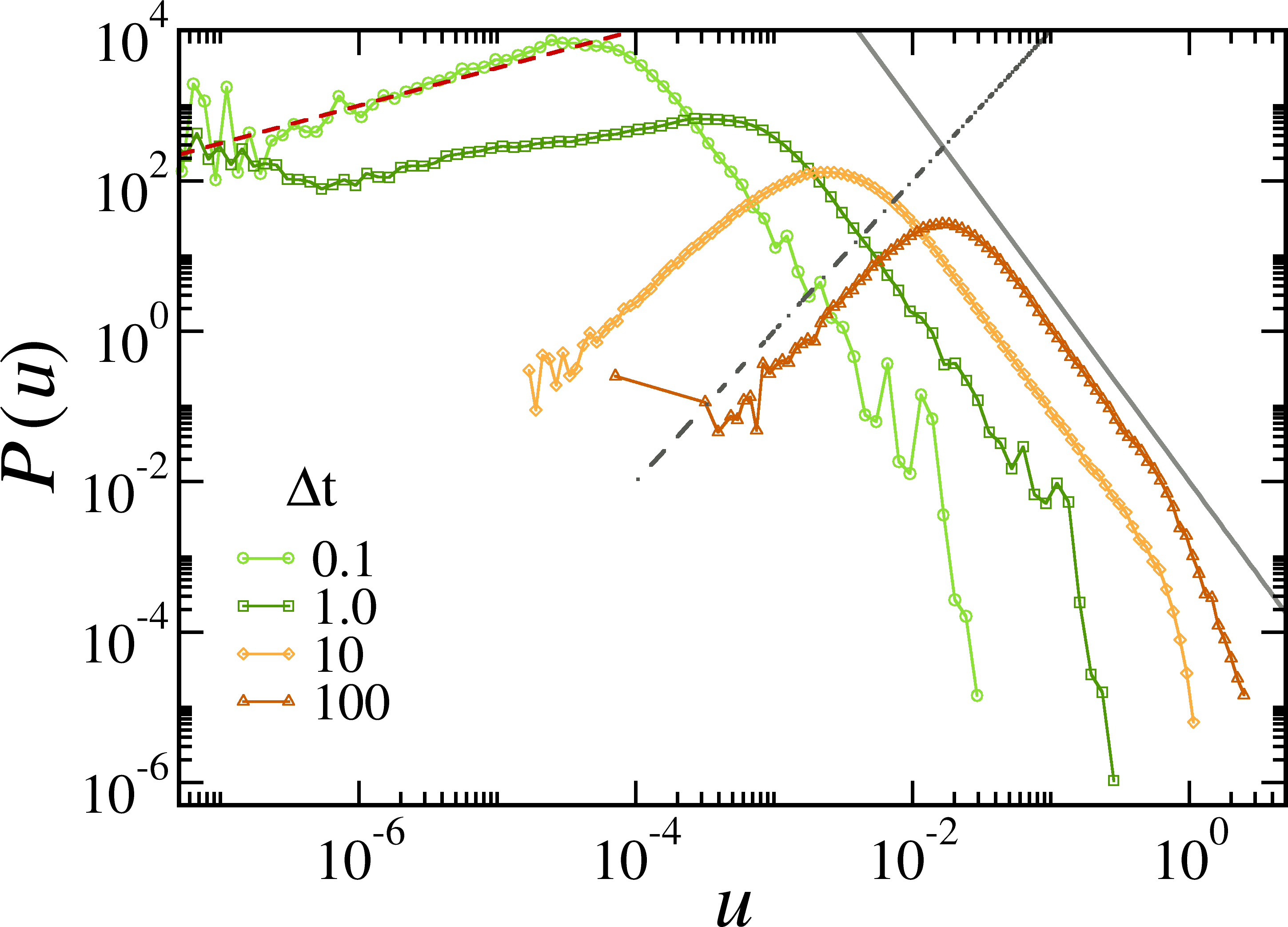
Figure 16 shows displacement distributions $P(u)$ for different definitions of the displacements $u$ at low plastic activity. In particular, we define $u$ as the tracer displacement in a time windows $\Delta t$. We show data for four different definitions $\Delta t=0.1,1.0,10.0$ and $100.0$. Notice that $\Delta t=0.1$ is the case used in Figs. 6 and 10. A favorable consequence of increasing $\Delta t$ is that the noisy peaks of the $P(u)$ tail at large $u$ smooth-out. On the other hand, the distribution shrink, the ranges of $u$ where power-laws could be fitted become thinner and we may evan loose some information about very small displacements. Still, even the largest $\Delta t$ shows clearly the power law tail at large displacements $\sim u^{-5/2}$, and $\sim u^{2}$ for the smallest displacements observed within that definition.

Displacement distribution of purely Brownian particles

The cases in which the movement of the tracer particles occurs only as a result of the thermal agitation (Brownian motion), display random trajectories. In that case, each displacement component ($u_{x}$, $u_{y}$, $u_{z}$) would populate a Gaussian distribution function. Therefore, the module of the displacement $u=\left(u_{x}^{2}+u_{y}^{2}+u_{z}^{2}\right)^{1/2}$ must follow a Maxwell-Boltzmann distribution,

$$P(u)=\sqrt{\frac{2}{\pi}}\frac{u^{2}}{c^{3}}\exp\left[-\frac{u^{2}}{2c^{2}}\right],$$ (21)

where $c$ is a scale parameter. Figure 17 shows a test simulation result for $P(u)$ for tracer particles that undergo only thermal agitation. As expected, a good accuracy with respect to Eq. 21 is seen.

When, either because of high plastic activity or because of high thermal agitation, the tracer’s movement is random-walk-like we expect to observe a $P(u)$ following Eq. 21, at least in a the displacement $u$ range where the movement is effectively Brownian.

Figure 17: Distribution of (the absolute value of) tracers displacements per unit time. The red squares correspond to a simulation of a pure Brownian motion, made with parameters $T=8.0\times 10^{-7}$, $L=32$. $u$ is defined as the displacement in $\Delta t=0.1$ units of time. The blue dashed line corresponds to the Maxwell-Boltzmann distribution (Eq. 21) with scale parameter c = 4.0$\times 10^{-4}$.

Appendix D Fully thermal system: variable activity

Figure 18: Mean square displacement $\left<r^{2}\right>$ for a varying temperature and plastic activity. The main plot shows the mean square displacement normalized by temperature as a function of time observation window for different temperatures, ranging from $T=6.0\times 10^{-6}$ (light-green curve) to $T=2.4\times 10^{-5}$ (dark-blue curve). The prefactor $B$ in Eq. 13 is fixed at $B=0.001$. The gray dashed-lines are guidelines to show the ($\sim t$) behavior. The inset shows $\left<r^{2}\right>$ unscaled. $\tau_{\tt ev}=20.0$. $\epsilon_{0}=0.1$. $L=32$.

The idea of a mean plastic activity that is insensitive to the external temperature is justified in cases where pre-stresses play a major role (e.g., in ‘as-quenched’ glasses). Nevertheless, one cannot rule out the case in which the same temperature is controlling the thermal agitation of particles and the plastic activity.

In this work we have considered a thermal agitation for tracers implemented as a Brownian dynamics (fully overdamped). Perhaps a more realistic approach would have been to use a Langevin dynamics (not necessarily fully overdamped). The control of the drag term might allow then to somehow decouple the “thermal agitation” temperature from the temperature parameter in the EP model. Although we haven’t explicitly used a new parameter for the drag term of the Brownian dynamics, the thermal agitation of the tracers and the temperature are relativized by the parameter “B” in the Arrhenius activation.

Figure 19: Dynamical structure factor $S(q,t)$ relaxation at short times and varying temperatures and activities. In all panels, the insets shows $S(q,t)$ as a function of $q^{2}$ for time windows up to $t=100$. The dark-red curve corresponds to duration of plastic events, $\tau_{\tt ev}=20$. $\epsilon_{0}$ = 0.1. $L=32$.

Mean square displacement varying activity.– In Fig. 18 we show the mean square displacement for different temperatures, where each temperature controls both the thermal agitation of the tracer particles and the probability of plastic events by thermal activation (we have used now a fixed $B=1\times 10^{-3}$ in Eq. 13). Now the influence of both sources of tracer particles agitation, plastic activity and temperature, is evidenced. In fact, one can better distinguish the crossover between two diffusive regimes previously insinuated in Fig. 7. At very low temperatures, plastic activity is almost absent or very spread and $\left<r^{2}\right>$ at short times becomes essentially dominated by the thermal agitation alone: particles diffuse with a diffusion coefficient $D\propto T$ (which is shown in the collapse of $\left<r^{2}\right>/T$ curves at short times  At higher temperatures, plastic activity becomes more and more important and eventually dominates the diffusion at large enough time windows. As a matter of fact, a $\left<r^{2}\right>/\left<a\right>$ scaling collapses the curves of higher temperatures at long times (not shown). In between the two diffusive regimes, we can notice a super-diffusive crossover. And even though it’s not easy to identify a ballistic regime, that super-diffusivity will already influence the relaxation shape exponents $\alpha$ and $\beta$. Finally, the crossover between the activity-dominated to the temperature-dominated diffusive regimes as we lower the temperature is understood by recalling that plastic activity decays much faster than temperature ($\left<a\right>\sim\exp(-1/T)$).

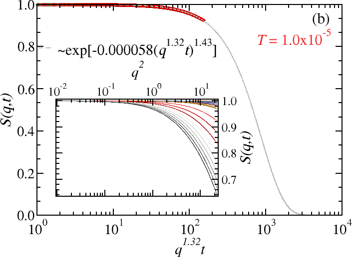
Dynamical structure factor varying activity.– Concerning the dynamical structure factor, as shown in Fig. 19, we now can see at short/intermediate times a compressed exponential behavior that turns to pure exponential as we decrease temperature. At contrast with the case in which the activity level is granted on non-thermal grounds, here the temperature decrease simply suppresses the plastic activity very fast and the few remaining persistent displacements of tracers easily disappear in a weak thermal agitation.

In contrast with what is observed in Fig. 9, now the decrease in temperature implies an increase in $\alpha$ towards $\alpha\simeq 2$, and, consistently, $\beta$ approaches 1 as we lower $T$. Even with a much weaker diffusive coefficient and therefore producing a much modest displacement and limited structure factor decay, for the lower temperature we obtain a nearly pure diffusive regime at short times (Fig. 19a): $S(q,t)\propto\exp\left[-A\left(q^{2}t\right)\right]$. One might say that at such low temperatures the tracers remain near their initial position doing a small local Brownian motion. They will eventually diffuse further away, but in our observation time window here, for the lowest temperatures they have barely traveled a distance comparable to the lattice cell. On the other hand, the compressed exponential is granted in the regime in which plastic activity dominates the relaxation. For the highest temperature (Fig. 19c) the structure factor decays as $S(q,t)\propto\exp\left[-A\left(q^{1.2}t\right)^{1.6}\right]$.

References

- Cipelletti et al. [2000a] L. Cipelletti, S. Manley, R. C. Ball, and D. A. Weitz, Phys. Rev. Lett. 84, 2275 (2000a).
- Ramos and Cipelletti [2001] L. Ramos and L. Cipelletti, Phys. Rev. Lett. 87, 245503 (2001).
- Cipelletti et al. [2003] L. Cipelletti, L. Ramos, S. Manley, E. Pitard, D. A. Weitz, E. E. Pashkovski, and M. Johansson, Faraday Discuss. 123, 237 (2003).
- Cipelletti and Ramos [2005] L. Cipelletti and L. Ramos, Journal of Physics: Condensed Matter 17, R253 (2005).
- Duri, A. and Cipelletti, L. [2006] Duri, A. and Cipelletti, L., Europhys. Lett. 76, 972 (2006).
- Caronna et al. [2008] C. Caronna, Y. Chushkin, A. Madsen, and A. Cupane, Phys. Rev. Lett. 100, 055702 (2008).
- Duri et al. [2009] A. Duri, T. Autenrieth, L.-M. Stadler, O. Leupold, Y. Chushkin, G. Grübel, and C. Gutt, Phys. Rev. Lett. 102, 145701 (2009).
- Angelini et al. [2013] R. Angelini, L. Zulian, A. Fluerasu, A. Madsen, G. Ruocco, and B. Ruzicka, Soft Matter 9, 10955 (2013).
- Trappe et al. [2007] V. Trappe, E. Pitard, L. Ramos, A. Robert, H. Bissig, and L. Cipelletti, Phys. Rev. E 76, 051404 (2007).
- Orsi et al. [2012] D. Orsi, L. Cristofolini, G. Baldi, and A. Madsen, Phys. Rev. Lett. 108, 105701 (2012).
- Ruta et al. [2012a] B. Ruta, Y. Chushkin, G. Monaco, L. Cipelletti, E. Pineda, P. Bruna, V. M. Giordano, and M. Gonzalez-Silveira, Phys. Rev. Lett. 109, 165701 (2012a).
- Ruta et al. [2013] B. Ruta, G. Baldi, G. Monaco, and Y. Chushkin, The Journal of Chemical Physics 138, 054508 (2013).
- Evenson et al. [2015] Z. Evenson, B. Ruta, S. Hechler, M. Stolpe, E. Pineda, I. Gallino, and R. Busch, Phys. Rev. Lett. 115, 175701 (2015).
- Ruta et al. [2017] B. Ruta, E. Pineda, and Z. Evenson, Journal of Physics: Condensed Matter 29, 503002 (2017).
- Tamborini et al. [2014] E. Tamborini, L. Cipelletti, and L. Ramos, Phys. Rev. Lett. 113, 078301 (2014).
- Bouchaud and Pitard [2001] J.-P. Bouchaud and E. Pitard, The European Physical Journal E 6, 231 (2001).
- Bouchaud and Pitard [2002] J.-P. Bouchaud and E. Pitard, The European Physical Journal E 9, 287 (2002).
- Bouchaud [2008] J.-P. Bouchaud, Anomalous relaxation in complex systems: From stretched to compressed exponentials, in Anomalous Transport (Wiley-VCH Verlag GmbH & Co. KGaA, 2008) pp. 327–345.
- Ferrero et al. [2014] E. E. Ferrero, K. Martens, and J.-L. Barrat, Phys. Rev. Lett. 113, 248301 (2014).
- Luo et al. [2017] P. Luo, P. Wen, H. Y. Bai, B. Ruta, and W. H. Wang, Phys. Rev. Lett. 118, 225901 (2017).
- Amini et al. [2021] N. Amini, F. Yang, E. Pineda, B. Ruta, M. Sprung, and A. Meyer, Phys. Rev. Materials 5, 055601 (2021).
- Song et al. [2022] J. Song, Q. Zhang, F. de Quesada, M. H. Rizvi, J. B. Tracy, J. Ilavsky, S. Narayanan, E. D. Gado, R. L. Leheny, N. Holten-Andersen, and G. H. McKinley, Proceedings of the National Academy of Sciences 119, e2201566119 (2022).
- Gabriel et al. [2015] J. Gabriel, T. Blochowicz, and B. Stühn, The Journal of Chemical Physics 142, 104902 (2015).
- Chaudhuri and Berthier [2017] P. Chaudhuri and L. Berthier, Phys. Rev. E 95, 060601 (2017).
- Bouzid et al. [2017] M. Bouzid, J. Colombo, L. V. Barbosa, and E. Del Gado, Nature communications 8, 1 (2017).
- Wu et al. [2018a] Z. W. Wu, W. Kob, W.-H. Wang, and L. Xu, Nature communications 9, 1 (2018a).
- Trachenko and Zaccone [2021] K. Trachenko and A. Zaccone, Journal of Physics: Condensed Matter 33, 315101 (2021).
- Lemaître [2014] A. Lemaître, Phys. Rev. Lett. 113, 245702 (2014).
- Chacko et al. [2019] R. N. Chacko, P. Sollich, and S. M. Fielding, Phys. Rev. Lett. 123, 108001 (2019).
- Lerbinger et al. [2022] M. Lerbinger, A. Barbot, D. Vandembroucq, and S. Patinet, Phys. Rev. Lett. 129, 195501 (2022).
- Note [1] Our model is not constructed to resolve the details of the dynamics occurring in the core of a relaxation event. Compared to particle-based dynamics, the short time dynamics of our model are on timescales larger than the typical beta-relaxation time of a glass-former and refer rather to the cage breaking regime. The persistent motion that we observe on “short time scales” is distinct from the commonly observed ballistic motion at times smaller than the beta relaxation time [60].
- Ruta et al. [2012b] B. Ruta, Y. Chushkin, G. Monaco, L. Cipelletti, E. Pineda, P. Bruna, V. M. Giordano, and M. Gonzalez-Silveira, Phys. Rev. Lett. 109, 165701 (2012b).
- Nicolas et al. [2018] A. Nicolas, E. E. Ferrero, K. Martens, and J.-L. Barrat, Rev. Mod. Phys. 90, 045006 (2018).
- Dyre et al. [1996] J. C. Dyre, N. B. Olsen, and T. Christensen, Phys. Rev. B 53, 2171 (1996).
- Dyre et al. [2006] J. C. Dyre, T. Christensen, and N. B. Olsen, Journal of Non-Crystalline Solids 352, 4635 (2006), proceedings of the 5th International Discussion Meeting on Relaxations in Complex Systems.
- Dyre [2006] J. C. Dyre, Rev. Mod. Phys. 78, 953 (2006).
- Ozawa and Biroli [2023] M. Ozawa and G. Biroli, Phys. Rev. Lett. 130, 138201 (2023).
- Falus et al. [2006] P. Falus, M. A. Borthwick, S. Narayanan, A. R. Sandy, and S. G. J. Mochrie, Phys. Rev. Lett. 97, 066102 (2006).
- Robert et al. [2006] A. Robert, E. Wandersman, E. Dubois, V. Dupuis, and R. Perzynski, Europhysics Letters (EPL) 75, 764 (2006).
- Chattoraj and Lemaître [2013] J. Chattoraj and A. Lemaître, Phys. Rev. Lett. 111, 066001 (2013).
- Lemaître [2015] A. Lemaître, The Journal of Chemical Physics 143, 164515 (2015).
- Jagla [2020] E. A. Jagla, Phys. Rev. E 101, 043004 (2020).
- Picard et al. [2004] G. Picard, A. Ajdari, F. Lequeux, and L. Bocquet, The European Physical Journal E 15, 371 (2004).
- Ferrero and Jagla [2019] E. E. Ferrero and E. A. Jagla, Soft Matter 15, 9041 (2019).
- Note [2] Rigorously speaking, its a bit more complicated than that, since we always keep track of both the probability of yielding in the ‘positive’ threshold and the probability of yielding in the ‘negative’ threshold . The complete definition being .
- Ferrero et al. [2021] E. E. Ferrero, A. B. Kolton, and E. A. Jagla, Phys. Rev. Materials 5, 115602 (2021).
- Note [3] We have checked nevertheless that the use of other values of , , does not affect our conclusions.
- Wang et al. [2022] X. J. Wang, Y. Z. Lu, X. Lu, J. T. Huo, Y. J. Wang, W. H. Wang, L. H. Dai, and M. Q. Jiang, Phys. Rev. E 105, 045003 (2022).
- Lu et al. [2018] Y. Z. Lu, M. Q. Jiang, X. Lu, Z. X. Qin, Y. J. Huang, and J. Shen, Phys. Rev. Appl. 9, 014023 (2018).
- Note [4] We expect our description to be compatible with one where the XPCS is observed at “large” values of , on a length-scale compatible with the size of the STZ. In fact, it was suggested that ISF measured at the peak of the structure factor reflects the behavior of the far fields of the van Hove correlation function [61]. In the EPMs this comes true by construction with the Eshelby propagator.
- Cipelletti et al. [2000b] L. Cipelletti, S. Manley, R. Ball, and D. Weitz, Physical review letters 84, 2275 (2000b).
- Ricci-Tersenghi and Zecchina [2000] F. Ricci-Tersenghi and R. Zecchina, Phys. Rev. E 62, R7567 (2000).
- Romá et al. [2006] F. Romá, S. Bustingorry, and P. M. Gleiser, Phys. Rev. Lett. 96, 167205 (2006).
- Ferrero et al. [2012] E. E. Ferrero, F. Romá, S. Bustingorry, and P. M. Gleiser, Phys. Rev. E 86, 031121 (2012).
- Note [5] The intermediate sub-diffusive, ‘statistical caging’ and associated stretched relaxation regime observed by some of us in ref. [19] turned out to be a feature of 2D systems only.
- Palmer et al. [1984] R. G. Palmer, D. L. Stein, E. Abrahams, and P. W. Anderson, Phys. Rev. Lett. 53, 958 (1984).
- Shang et al. [2019] B. Shang, J. Rottler, P. Guan, and J.-L. Barrat, Phys. Rev. Lett. 122, 105501 (2019).
- Cornet et al. [2023] A. Cornet, G. Garbarino, F. Zontone, Y. Chushkin, J. Jacobs, E. Pineda, T. Deschamps, S. Li, A. Ronca, J. Shen, G. Morard, N. Neuber, M. Frey, R. Busch, I. Gallino, M. Mezouar, G. Vaughan, and B. Ruta, Acta Materialia 255, 119065 (2023).
- Note [6] Note that the use of an inertial dynamics for the tracers (instead of a fully overdamped one) would change the behavior of the curves at short times.
- Karmakar [2016] S. Karmakar, Journal of Physics: Conference Series 759, 012008 (2016).
- Wu et al. [2018b] B. Wu, T. Iwashita, and T. Egami, Phys. Rev. Lett. 120, 135502 (2018b).