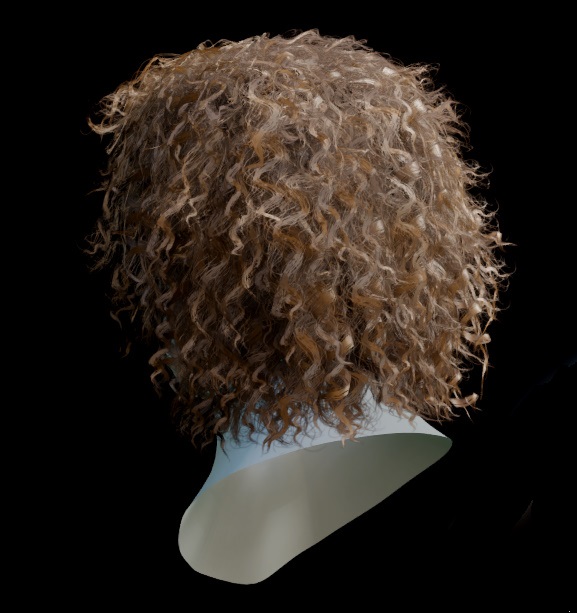
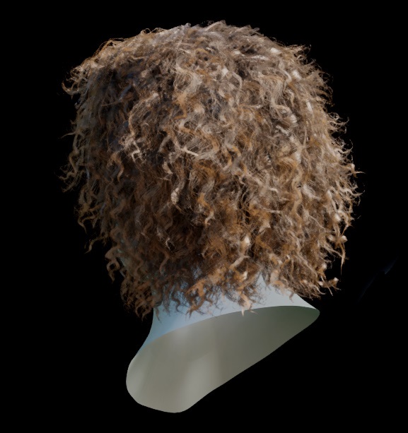
Fast Real-Time Shading for Polygonal Hair

Martin Gerard
Eko Software

1.   Introduction

Hair is one of the most difficult material to render in real-time, yet an extremely important visual component of characters and can easily break immersion if not done properly. This has lead for artists and programmers to come up with various solutions that in some cases require careful tweaking in order to achieve the desired realism in the dedicated time budget, and add a significant amount of time-consuming work for both artists and programmers. Most of these techniques require to maintain data structures at run-time, like deep opacity maps, to represent volumetric self-shadowing and can be costly.

In this paper, we present a novel method for shading hair realistically with dynamic lights or a GI system in a single pass, without having to maintain a dedicated data structure, and without the need of additional textures other than a diffuse map and a flow map.

Our work builds upon the model of a phase function of a single hair by [Marschner et al.] through the addition of a self-shadowing term baked in the geometry and a technique for a fast integration of the model over an environment map.

2.   The hair rendering equation

Let’s begin by writing the rendering equation for a hair of tangent u𝑢u

Lout(x,ωo)=ΩLin(x,ωi)S(ωi,ωo,u)𝑑ωisubscript𝐿𝑜𝑢𝑡𝑥subscript𝜔𝑜subscriptΩsubscript𝐿𝑖𝑛𝑥subscript𝜔𝑖𝑆subscript𝜔𝑖subscript𝜔𝑜𝑢differential-dsubscript𝜔𝑖\begin{multlined}L_{out}(x,\omega_{o})=\int_{\Omega}{L_{in}(x,\omega_{i})S(\omega_{i},\omega_{o},u)d\omega_{i}}\end{multlined}L_{out}(x,\omega_{o})=\int_{\Omega}{L_{in}(x,\omega_{i})S(\omega_{i},\omega_{o},u)d\omega_{i}} (1)

Lout(x,ωo)subscript𝐿𝑜𝑢𝑡𝑥subscript𝜔𝑜L_{out}(x,\omega_{o}) and Lin(x,ωi)subscript𝐿𝑖𝑛𝑥subscript𝜔𝑖L_{in}(x,\omega_{i}) are respectively the radiance going out of point x𝑥x in direction ωosubscript𝜔𝑜\omega_{o} and the radiance coming to x from direction ωisubscript𝜔𝑖\omega_{i}. S(ωo,ωi,u(x))𝑆subscript𝜔𝑜subscript𝜔𝑖𝑢𝑥S(\omega_{o},\omega_{i},u(x)) is the single-hair phase function expressing the fraction of the light coming from direction ωisubscript𝜔𝑖\omega_{i} that gets scattered in direction ωosubscript𝜔𝑜\omega_{o} by a hair of tangent u𝑢u.

We approximate the input radiance field Lin(x,ωi)subscript𝐿𝑖𝑛𝑥subscript𝜔𝑖L_{in}(x,\omega_{i}) by the product of a far field Lfar(ωi)subscript𝐿𝑓𝑎𝑟subscript𝜔𝑖L_{far}(\omega_{i}) with a near field transmittance function V(x,ωi)𝑉𝑥subscript𝜔𝑖V(x,\omega_{i}):

Lin(x,ωi)=Lfar(x,ωi)V(x,ωi)subscript𝐿𝑖𝑛𝑥subscript𝜔𝑖subscript𝐿𝑓𝑎𝑟𝑥subscript𝜔𝑖𝑉𝑥subscript𝜔𝑖L_{in}(x,\omega_{i})=L_{far}(x,\omega_{i})V(x,\omega_{i}) (2)

The rendering equation becomes:

Lout(x,ωo)=ΩLfar(x,ωi)V(x,ωi)S(ωi,ωo,u)𝑑ωisubscript𝐿𝑜𝑢𝑡𝑥subscript𝜔𝑜subscriptΩsubscript𝐿𝑓𝑎𝑟𝑥subscript𝜔𝑖𝑉𝑥subscript𝜔𝑖𝑆subscript𝜔𝑖subscript𝜔𝑜𝑢differential-dsubscript𝜔𝑖\begin{multlined}L_{out}(x,\omega_{o})=\int_{\Omega}{L_{far}(x,\omega_{i})V(x,\omega_{i})S(\omega_{i},\omega_{o},u)d\omega_{i}}\end{multlined}L_{out}(x,\omega_{o})=\int_{\Omega}{L_{far}(x,\omega_{i})V(x,\omega_{i})S(\omega_{i},\omega_{o},u)d\omega_{i}} (3)

2.1.   The single hair phase function

Let’s focus first on the single-hair phase function S(ωi,ωo,u)𝑆subscript𝜔𝑖subscript𝜔𝑜𝑢S(\omega_{i},\omega_{o},u)
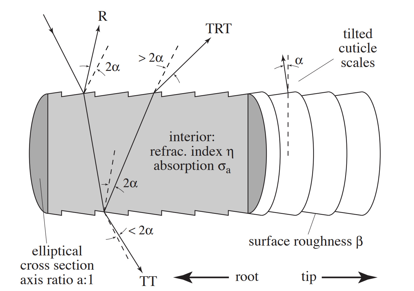
Refer to caption
Figure 1: A schematic of our model for a hair fiber. The dashed lines indicate the scattering angles for a cylinder without tilted surface scales.

In [Marschner et al.], the authors separate the phase function in three terms, corresponding to the light directly reflected on the surface of the hair (the R mode), the light transmitted into the hair then transmitted out of the hair through the other side (the TT mode), and the light transmitted into the hair, reflected on the inner surface of the hair then transmitted outside of the hair (the TRT mode) as represented in figure 1.
Refer to caption
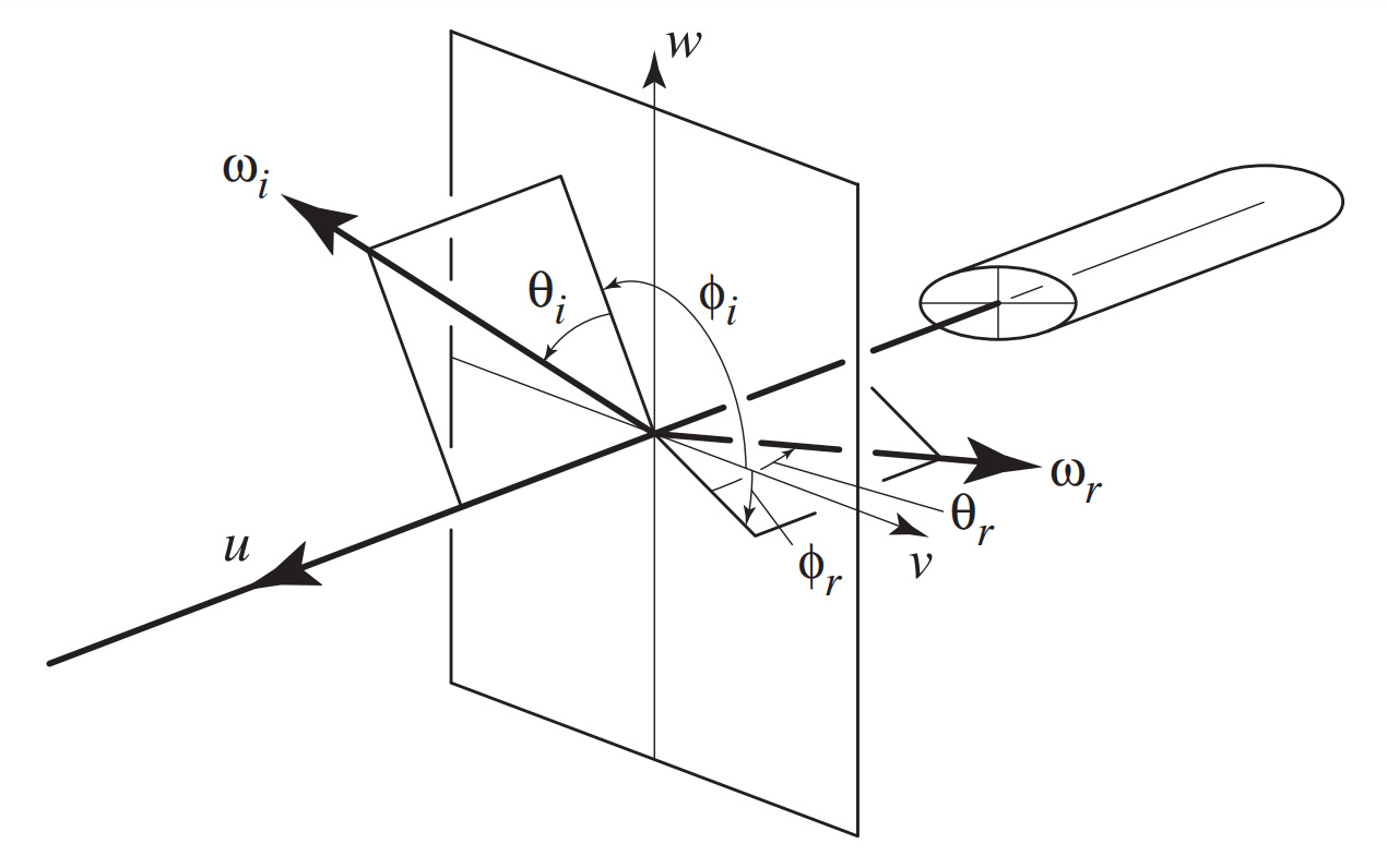
Figure 2: Notation for scattering geometry

We denote by ϕisubscriptitalic-ϕ𝑖\phi_{i} and ϕrsubscriptitalic-ϕ𝑟\phi_{r} the azimuthal angle of the incident ray and the outgoing ray in the normal plane of the hair. θisubscript𝜃𝑖\theta_{i} and θrsubscript𝜃𝑟\theta_{r} refer to the inclination of the same rays with respect to the normal plane. We will also define the difference angle θd=(θrθi)/2subscript𝜃𝑑subscript𝜃𝑟subscript𝜃𝑖2\theta_{d}=(\theta_{r}-\theta_{i})/2, the half angles θh=(θi+θr)/2subscript𝜃subscript𝜃𝑖subscript𝜃𝑟2\theta_{h}=(\theta_{i}+\theta_{r})/2 and ϕh=(ϕi+ϕr)/2subscriptitalic-ϕsubscriptitalic-ϕ𝑖subscriptitalic-ϕ𝑟2\phi_{h}=(\phi_{i}+\phi_{r})/2 and the relative azimuth ϕ=ϕrϕiitalic-ϕsubscriptitalic-ϕ𝑟subscriptitalic-ϕ𝑖\phi=\phi_{r}-\phi_{i} . The angles are drawn in figure 2.

In these conditions, [Marschner et al.] shows that the phase function S(ωi,ωr,u)𝑆subscript𝜔𝑖subscript𝜔𝑟𝑢S(\omega_{i},\omega_{r},u) can be expressed as

S(ωi,ωr,u)𝑆subscript𝜔𝑖subscript𝜔𝑟𝑢\displaystyle S(\omega_{i},\omega_{r},u) =\displaystyle= (4)
MR(θh)NR(η,θd,ϕ)/cos2θd+limit-fromsubscript𝑀𝑅subscript𝜃subscript𝑁𝑅𝜂subscript𝜃𝑑italic-ϕ𝑐𝑜superscript𝑠2subscript𝜃𝑑\displaystyle M_{R}(\theta_{h})N_{R}(\eta,\theta_{d},\phi)/cos^{2}\theta_{d}+
MTT(θh)NTT(θd,ϕ)/cos2θd+limit-fromsubscript𝑀𝑇𝑇subscript𝜃subscript𝑁𝑇𝑇subscript𝜃𝑑italic-ϕ𝑐𝑜superscript𝑠2subscript𝜃𝑑\displaystyle M_{TT}(\theta_{h})N_{TT}(\theta_{d},\phi)/cos^{2}\theta_{d}+
MTRT(θh)NTRT(θd,ϕ)/cos2θdsubscript𝑀𝑇𝑅𝑇subscript𝜃subscript𝑁𝑇𝑅𝑇subscript𝜃𝑑italic-ϕ𝑐𝑜superscript𝑠2subscript𝜃𝑑\displaystyle M_{TRT}(\theta_{h})N_{TRT}(\theta_{d},\phi)/cos^{2}\theta_{d}

where MRsubscript𝑀𝑅M_{R}, MTTsubscript𝑀𝑇𝑇M_{TT} and MTRTsubscript𝑀𝑇𝑅𝑇M_{TRT} are the three following longitudinal functions

MR(θh)subscript𝑀𝑅subscript𝜃\displaystyle M_{R}(\theta_{h}) =𝒢(βR,θhαR)absent𝒢subscript𝛽𝑅subscript𝜃subscript𝛼𝑅\displaystyle=\mathcal{G}(\beta_{R},\theta_{h}-\alpha_{R}) (5)
MTT(θh)subscript𝑀𝑇𝑇subscript𝜃\displaystyle M_{TT}(\theta_{h}) =𝒢(βTT,θhαTT)absent𝒢subscript𝛽𝑇𝑇subscript𝜃subscript𝛼𝑇𝑇\displaystyle=\mathcal{G}(\beta_{TT},\theta_{h}-\alpha_{TT})
MTRT(θh)subscript𝑀𝑇𝑅𝑇subscript𝜃\displaystyle M_{TRT}(\theta_{h}) =𝒢(βTRT,θhαTRT)absent𝒢subscript𝛽𝑇𝑅𝑇subscript𝜃subscript𝛼𝑇𝑅𝑇\displaystyle=\mathcal{G}(\beta_{TRT},\theta_{h}-\alpha_{TRT})

where 𝒢(β,x)𝒢𝛽𝑥\mathcal{G}(\beta,x) is a unit-integral, zero-mean lobe function of width β𝛽\beta. We chose to use a Henyey-Greenstein function width β𝛽\beta, which is faster to compute than a Gaussian.

𝒢(β,cosθh)=14π1g(β)2(1+g(β)22g(β)cosθh)32𝒢𝛽𝑐𝑜𝑠subscript𝜃14𝜋1𝑔superscript𝛽2superscript1𝑔superscript𝛽22𝑔𝛽𝑐𝑜𝑠subscript𝜃32\mathcal{G}(\beta,cos\theta_{h})=\frac{1}{4\pi}\frac{1-g(\beta)^{2}}{(1+g(\beta)^{2}-2g(\beta)cos\theta_{h})^{\frac{3}{2}}} (6)

[Marschner et al.] gives the following surface values

βR=5° to 10°βTT=βR/2βTRT=2βR and αR=5° to 10°αTT=αR/2αTRT=3αR/2subscript𝛽𝑅absent5° to 10°subscript𝛽𝑇𝑇absentsubscript𝛽𝑅2subscript𝛽𝑇𝑅𝑇absent2subscript𝛽𝑅 and subscript𝛼𝑅absent5° to 10°subscript𝛼𝑇𝑇absentsubscript𝛼𝑅2subscript𝛼𝑇𝑅𝑇absent3subscript𝛼𝑅2\begin{aligned} \beta_{R}&=5\degree\textrm{ to }10\degree\\ \beta_{TT}&=\beta_{R}/2\\ \beta_{TRT}&=2\beta_{R}\end{aligned}\textrm{ and }\begin{aligned} \alpha_{R}&=-5\degree\textrm{ to }-10\degree\\ \alpha_{TT}&=-\alpha_{R}/2\\ \alpha_{TRT}&=-3\alpha_{R}/2\\ \end{aligned}

For βR=10°subscript𝛽𝑅10°\beta_{R}=10\degree and αR=10°subscript𝛼𝑅10°\alpha_{R}=-10\degree, we find the following values for g(β)𝑔𝛽g(\beta) by minimizing the L2subscript𝐿2L_{2} norm of the difference between 𝒢𝒢\mathcal{G} and a gaussian.

g(βR)𝑔subscript𝛽𝑅\displaystyle g(\beta_{R}) =0.752absent0.752\displaystyle=0.752
g(βTT)𝑔subscript𝛽𝑇𝑇\displaystyle g(\beta_{TT}) =0.865absent0.865\displaystyle=0.865
g(βTRT)𝑔subscript𝛽𝑇𝑅𝑇\displaystyle g(\beta_{TRT}) =0.578absent0.578\displaystyle=0.578

The azimuthal part N(θd,ϕ)𝑁subscript𝜃𝑑italic-ϕN(\theta_{d},\phi) is detailed in [Marschner et al.] and is to costly to evaluate analytically. We use the following approximation

Np(θd,ϕ)subscript𝑁𝑝subscript𝜃𝑑italic-ϕ\displaystyle N_{p}(\theta_{d},\phi) =Np,LUT(θd,ϕ)T(σa,hmax)pabsentsubscript𝑁𝑝𝐿𝑈𝑇subscript𝜃𝑑italic-ϕ𝑇superscriptsubscript𝜎𝑎subscript𝑚𝑎𝑥𝑝\displaystyle=N_{p,LUT}(\theta_{d},\phi)T(\sigma_{a},h_{max})^{p} (7)

where Np,LUTsubscript𝑁𝑝𝐿𝑈𝑇N_{p,LUT} is a look-up texture generated using the algorithms described by [Marschner et al.], σasubscript𝜎𝑎\sigma_{a} is the colored absorption of the hair and hmaxsubscript𝑚𝑎𝑥h_{max} is the offset of the incident light from the fiber that maximizes T(σa,h)𝑇subscript𝜎𝑎T(\sigma_{a},h). We get

NR(θd,ϕ)subscript𝑁𝑅subscript𝜃𝑑italic-ϕ\displaystyle N_{R}(\theta_{d},\phi) =NR,LUT(θd,ϕ)absentsubscript𝑁𝑅𝐿𝑈𝑇subscript𝜃𝑑italic-ϕ\displaystyle=N_{R,LUT}(\theta_{d},\phi) (8)
NTT(θd,ϕ)subscript𝑁𝑇𝑇subscript𝜃𝑑italic-ϕ\displaystyle N_{TT}(\theta_{d},\phi) =NTT,LUT(θd,ϕ)e4σaabsentsubscript𝑁𝑇𝑇𝐿𝑈𝑇subscript𝜃𝑑italic-ϕsuperscript𝑒4subscript𝜎𝑎\displaystyle=N_{TT,LUT}(\theta_{d},\phi)e^{-4\sigma_{a}}
NTRT(θd,ϕ)subscript𝑁𝑇𝑅𝑇subscript𝜃𝑑italic-ϕ\displaystyle N_{TRT}(\theta_{d},\phi) =NTRT,LUT(θd,ϕ)e8σa(132η2)absentsubscript𝑁𝑇𝑅𝑇𝐿𝑈𝑇subscript𝜃𝑑italic-ϕsuperscript𝑒8subscript𝜎𝑎132superscript𝜂2\displaystyle=N_{TRT,LUT}(\theta_{d},\phi)e^{-8\sigma_{a}(1-\frac{3}{2\eta^{2}})}
where
η𝜂\displaystyle\eta =1.552cos2θd+1cosθdabsentsuperscript1.552𝑐𝑜superscript𝑠2subscript𝜃𝑑1𝑐𝑜𝑠subscript𝜃𝑑\displaystyle=\sqrt{\frac{1.55^{2}-cos^{2}\theta_{d}+1}{cos\theta_{d}}}

2.2.   Per-vertex near field transmittance

We now have a mean to evaluate the phase function for a single hair, but it doesn’t take into account the presence of surrounding hair. For simplicity, we don’t take multiple scattering into account, and simply focus on the occlusion of the light from the surrounding hair. This allows us to consider a function V(ωi)𝑉subscript𝜔𝑖V(\omega_{i}) that only depends on the geometry itself and thus can be precomputed for static hair. One could object that hair are rarely static but we find that the precomputed data still give plausible results for small deformations.

We precompute the near field transmittance by rendering a cubemap for each vertex that stores the transmittance for each direction using alpha blending. A transmittance of 1 means that the vertex is unoccluded in that direction whereas a transmittance of 0 means that it is entirely shadowed. We then store a spherical harmonics approximation of the cubemap in the vertex attributes.

At runtime, we extract the spherical harmonics coefficients in the vertex shader and rotate them to take into account the hair orientation before passing them to the pixel shader.

This technique allows us to evaluate the obstruction of light by the surrounding hair at any point in any given direction simply by decompressing the vertex attributes, without having to render deep opacity maps for every light.

2.3.   Direct lighting

For a point light or a directional light, the lighting equation simplifies to

Ldirect(ωo,x)=Llight(x)V(ωl,x)S(ωo,ωl,u)subscript𝐿𝑑𝑖𝑟𝑒𝑐𝑡subscript𝜔𝑜𝑥subscript𝐿𝑙𝑖𝑔𝑡𝑥𝑉subscript𝜔𝑙𝑥𝑆subscript𝜔𝑜subscript𝜔𝑙𝑢L_{direct}(\omega_{o},x)=L_{light}(x)V(\omega_{l},x)S(\omega_{o},\omega_{l},u) (9)

where Llight(x)subscript𝐿𝑙𝑖𝑔𝑡𝑥L_{light}(x) is the radiance that would be received from the light at point x𝑥x if there were no hair, and ωlsubscript𝜔𝑙\omega_{l} is the direction from the point x𝑥x to the light. V(ωl,x)𝑉subscript𝜔𝑙𝑥V(\omega_{l},x) can be evaluated directly from its spherical harmonics decomposition.

With a low order approximation of V𝑉V, the overestimation of V𝑉V applied to the transmission mode can produce undesirable light leaking from back lights, in that case, this issue can be alleviated by introducing a bias such that

V~(ωl,x)=max(0,V(ωl,x)bias1bias)~𝑉subscript𝜔𝑙𝑥𝑚𝑎𝑥0𝑉subscript𝜔𝑙𝑥𝑏𝑖𝑎𝑠1𝑏𝑖𝑎𝑠\tilde{V}(\omega_{l},x)=max\left(0,\frac{V(\omega_{l},x)-bias}{1-bias}\right) (10)

2.4.   Integration over the far field

In what follows, we will assume that we have access to a spherical harmonics representation of the far field. Given that the transmittance function V𝑉V is already expressed as spherical harmonics, we propose to decompose the phase function in spherical harmonics so that the rendering equation can be reduced to the integral of the product of three spherical harmonics, which can thus be computed as a combination of their coefficients.

Sωr(ωi)=SωrR(ωi)+SωrTT(ωi,σa)+SωrTRT(ωi,σa)subscript𝑆subscript𝜔𝑟subscript𝜔𝑖subscriptsuperscript𝑆𝑅subscript𝜔𝑟subscript𝜔𝑖subscriptsuperscript𝑆𝑇𝑇subscript𝜔𝑟subscript𝜔𝑖subscript𝜎𝑎subscriptsuperscript𝑆𝑇𝑅𝑇subscript𝜔𝑟subscript𝜔𝑖subscript𝜎𝑎S_{\omega_{r}}(\omega_{i})=S^{R}_{\omega_{r}}(\omega_{i})+S^{TT}_{\omega_{r}}(\omega_{i},\sigma_{a})+S^{TRT}_{\omega_{r}}(\omega_{i},\sigma_{a}) (11)

It follows from equation 8 that

SωrTT(ωi,σa)=SωrTT(ωi)e4σasubscriptsuperscript𝑆𝑇𝑇subscript𝜔𝑟subscript𝜔𝑖subscript𝜎𝑎subscriptsuperscript𝑆𝑇𝑇subscript𝜔𝑟subscript𝜔𝑖superscript𝑒4subscript𝜎𝑎S^{TT}_{\omega_{r}}(\omega_{i},\sigma_{a})=S^{TT}_{\omega_{r}}(\omega_{i})e^{-4\sigma_{a}} (12)

We find that the SωrTRTsubscriptsuperscript𝑆𝑇𝑅𝑇subscript𝜔𝑟S^{TRT}_{\omega_{r}} can be approximated by

SωrTRT(ωi,σa)=SωrTRT(ωi)e112σasubscriptsuperscript𝑆𝑇𝑅𝑇subscript𝜔𝑟subscript𝜔𝑖subscript𝜎𝑎subscriptsuperscript𝑆𝑇𝑅𝑇subscript𝜔𝑟subscript𝜔𝑖superscript𝑒112subscript𝜎𝑎S^{TRT}_{\omega_{r}}(\omega_{i},\sigma_{a})=S^{TRT}_{\omega_{r}}(\omega_{i})e^{-\frac{11}{2}\sigma_{a}} (13)

So that

Sωr(ωi)=SωrR(ωi)+SωrTT(ωi)e4σa+SωrTRT(ωi)e112σasubscript𝑆subscript𝜔𝑟subscript𝜔𝑖subscriptsuperscript𝑆𝑅subscript𝜔𝑟subscript𝜔𝑖subscriptsuperscript𝑆𝑇𝑇subscript𝜔𝑟subscript𝜔𝑖superscript𝑒4subscript𝜎𝑎subscriptsuperscript𝑆𝑇𝑅𝑇subscript𝜔𝑟subscript𝜔𝑖superscript𝑒112subscript𝜎𝑎S_{\omega_{r}}(\omega_{i})=S^{R}_{\omega_{r}}(\omega_{i})+S^{TT}_{\omega_{r}}(\omega_{i})e^{-4\sigma_{a}}+S^{TRT}_{\omega_{r}}(\omega_{i})e^{-\frac{11}{2}\sigma_{a}} (14)

Let aωrRsubscriptsuperscript𝑎𝑅subscript𝜔𝑟a^{R}_{\omega_{r}}, aωrTTsubscriptsuperscript𝑎𝑇𝑇subscript𝜔𝑟a^{TT}_{\omega_{r}} and aωrTRTsubscriptsuperscript𝑎𝑇𝑅𝑇subscript𝜔𝑟a^{TRT}_{\omega_{r}} be the coefficients of the spherical harmonics decomposition of SωrRsubscriptsuperscript𝑆𝑅subscript𝜔𝑟S^{R}_{\omega_{r}}, SωrTTsubscriptsuperscript𝑆𝑇𝑇subscript𝜔𝑟S^{TT}_{\omega_{r}} and SωrTRTsubscriptsuperscript𝑆𝑇𝑅𝑇subscript𝜔𝑟S^{TRT}_{\omega_{r}} respectively, then

Sωr(ωi)=[aωrR+aωrTTe4σa+aωrTRTe112σa]Ylm(ωi)subscript𝑆subscript𝜔𝑟subscript𝜔𝑖delimited-[]subscriptsuperscript𝑎𝑅subscript𝜔𝑟subscriptsuperscript𝑎𝑇𝑇subscript𝜔𝑟superscript𝑒4subscript𝜎𝑎subscriptsuperscript𝑎𝑇𝑅𝑇subscript𝜔𝑟superscript𝑒112subscript𝜎𝑎subscript𝑌𝑙𝑚subscript𝜔𝑖S_{\omega_{r}}(\omega_{i})=\sum\left[a^{R}_{\omega_{r}}+a^{TT}_{\omega_{r}}e^{-4\sigma_{a}}+a^{TRT}_{\omega_{r}}e^{-\frac{11}{2}\sigma_{a}}\right]Y_{lm}(\omega_{i}) (15)
Kajiya-Kay + Ambient term Ours Ground Truth
Environment map Refer to caption Refer to caption Refer to caption
Environment map + Directional light Refer to caption Refer to caption Refer to caption
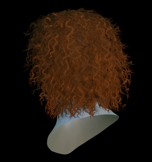
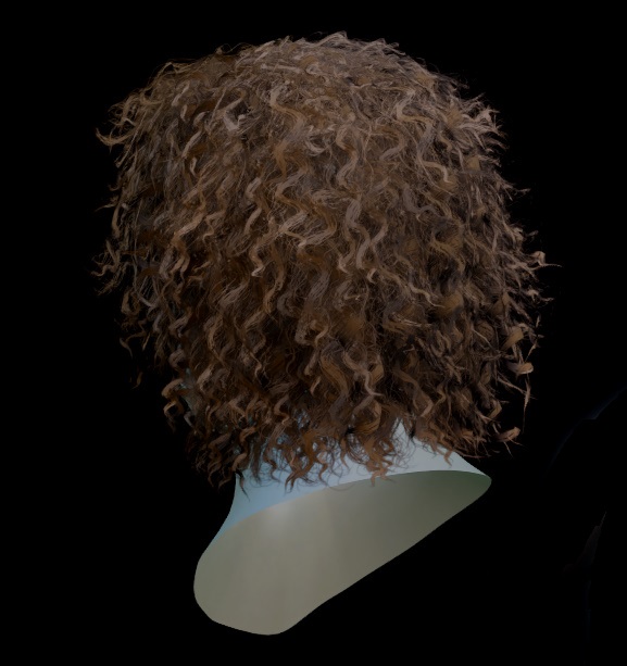
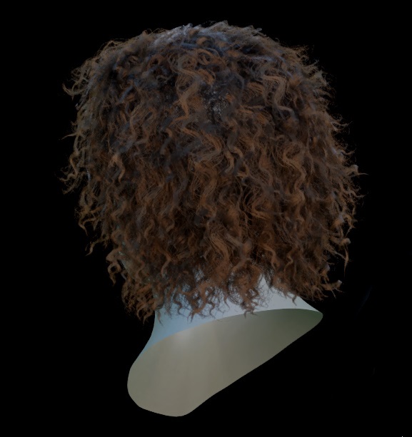
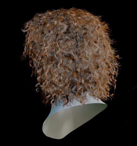
Figure 3: Polygonal hair rendered with our technique versus Kajiya-Kay in a comparable amount of time. We compare it to a path-traced reference render using the single scattering approximation.

aRsuperscript𝑎𝑅a^{R}, aTTsuperscript𝑎𝑇𝑇a^{TT} and aTRTsuperscript𝑎𝑇𝑅𝑇a^{TRT} are scalar functions of ωrsubscript𝜔𝑟\omega_{r} and can be precomputed. By choosing to express the coefficients in a base where the hair tangent u𝑢u is pointing up, we can store each coefficient in a 1D look-up texture parametrized by sin(θr)𝑠𝑖𝑛subscript𝜃𝑟sin(\theta_{r}).

At runtime, we can sample the look-up texture, rotate the coefficients back to world space, then evaluate the triple product integral as a sum of integrals of spherical harmonics that can be computed using Wigner 3-j symbols in the following way

ΩYl1m1(ω)Yl2m2(ω)Yl3m3(ω)𝑑ω=(2l1+1)(2l2+1)(2l3+1)4π(l1l2l3000)(l1l2l3m1m2m3)subscriptΩsubscript𝑌subscript𝑙1subscript𝑚1𝜔subscript𝑌subscript𝑙2subscript𝑚2𝜔subscript𝑌subscript𝑙3subscript𝑚3𝜔differential-d𝜔2subscript𝑙112subscript𝑙212subscript𝑙314𝜋matrixsubscript𝑙1subscript𝑙2subscript𝑙3000matrixsubscript𝑙1subscript𝑙2subscript𝑙3subscript𝑚1subscript𝑚2subscript𝑚3\begin{split}&\int_{\Omega}Y_{l_{1}m_{1}}(\omega)Y_{l_{2}m_{2}}(\omega)Y_{l_{3}m_{3}}(\omega)d\omega=\\ &\sqrt{\frac{(2l_{1}+1)(2l_{2}+1)(2l_{3}+1)}{4\pi}}\begin{pmatrix}l_{1}&l_{2}&l_{3}\\ 0&0&0\\ \end{pmatrix}\begin{pmatrix}l_{1}&l_{2}&l_{3}\\ m_{1}&m_{2}&m_{3}\\ \end{pmatrix}\end{split} (16)

3.   Implementation

We used 2-band SH (9 scalar coefficients) for V𝑉V encoded in the vertex attributes and 1-band SH for the phase function. The phase function look-up texture is a 128x3 8bits normalized RGBA texture, parametrized by (sin(θr)+1)/2𝑠𝑖𝑛subscript𝜃𝑟12(sin(\theta_{r})+1)/2 in x. For hair transparency, we used Adaptive Transparency by [Salvi and al.] with 4 nodes.

Kayija-Kay Ours
Curly hair (9K tri) Close up 0.138 ms 0.316 ms
Long curly hair (34K tri) Close up 0.248 ms 0.458 ms
Curly hair (9K tri) Larger shot 0.036 ms 0.068 ms
Long curly hair (34K tri) Larger shot 0.040 ms 0.081 ms
Figure 4: Render time of two hair model in close up at 1080p on a NVIDIA RTX 3080 with our technique.

4.   Results

We use a path-traced reference which we call "ground truth" (without taking into account multiple scattering) which we compare against our technique in Fig. 3.

All results are measured on a NVIDIA RTX 3080 at 1080p with two different scene settings. The first setting is a close up shot, where the hair itself covers a surface of approximately 600x600 pixels whereas the second setting is a larger shot, more representative of a common case in a video game where the hair covers a surface of approximately 150x150 pixels. In both case, the hair are lit by an environment map and a directional light. We compare our timings with [J. Kajiya and T. Kay]’s shading in the same conditions. The results are shown in Fig. 4 and show that our technique is not significantly more expensive than [J. Kajiya and T. Kay] (which is broadly used for being fast) while simulating more features, without the overhead cost of having to render deep opacity maps or maintaining another data structure.

5.   Conclusions

In this paper we have presented a fast way of solving the hair rending equation at runtime without maintaining a data structure. The visual result, while preserving the main features of the path-traced reference, still exhibits some differences that can be reduced by increasing the order of the spherical harmonics as needed.

References

  • [Marschner et al.] Stephen R. Marschner, Henrik Wann Jensen and Mike Cammarano (2003). Light Scattering from Human Hair Fibers. ACM Transactions On Graphics, 22,3:780-791.
  • [Salvi and al.] Marco Salvi, Jefferson Montgomery and Aaron Lefohn (2011). Adaptive Transparency. Conference: Proceedings of the ACM SIGGRAPH/EUROGRAPHICS Conference on High Performance Graphics 2011, Vancouver, Canada, August 5-7, 2011.
  • [J. Kajiya and T. Kay] J. Kajiya and T. Kay (1989). Rendering fur with three dimensional textures. In SIGGRAPH 89 Conference Proceedings, pp. 271-280, 1989..