Analysis of the Effects of Curvature on the Solutions of Shallow Water Equations

Abstract

The most used form of the Shallow Water Equations doesn’t take into account the variation of the curvature of the base flow surface. In this paper, we compare the theoretical and numerical solutions of the standard model and with the solutions of an extended model and for a large class of base flow surfaces. We find that the solution of the standard model is still a good approximation for the extended model for many real life applications.
Keywords: multiphysics, complex dynamics, PDEs, numerical simulation, stationary solution.
2020 MSC: 35Q35, 35L60, 76-10, 53Z05.

1 Introduction

For a large number of applications, especially for the ones in hydrology [1, 2, 3, 4], the mathematical model of the water flow on the soil surface is given by (S-SWE)

$$\begin{split}\displaystyle\frac{\partial h}{\partial t}+\partial_{j}\left(hv^{j}\right)&=\mathfrak{M},\\ \displaystyle\frac{\partial(hv_{i})}{\partial t}+\partial_{j}\left(hv_{i}v^{j}\right)+h\partial_{i}w&=\mathfrak{F}_{i},\quad i=1,2,\end{split}$$ (1)

where $h(t,\boldsymbol{x})$ is the water depth and $v_{i}(t,\boldsymbol{x})$ and $v^{i}(t,\boldsymbol{x})$ are the covariant and contravariant components of the water velocity $\boldsymbol{v}(t,\boldsymbol{x})$. We used here the Einstein summation convention for writing the model i n this compact form. The potential of the water level is

$$w=g\left[z(\boldsymbol{x})+h(t,\boldsymbol{x})\right],$$

where $z(\boldsymbol{x})$ is the altitude of the soil surface and $g$ represents the gravitational acceleration. The contribution of rain and infiltration to the water mass balance is taken into consideration through $\mathfrak{M}$, while $\mathfrak{F}_{i}$ quantify the rates of momentum production (they can include plant cover resistance and fluid-soil friction, for example).

2 Shallow Water Equations for Surface with Variable Curvature, E-SWE

If the base surface of the flow exhibits different orientations or moderate variations of the geometrical properties of its metrics, then it is convenient (at least from a theoretical point of view) to work with a surface base coordinate system. Let us assume that the base flow surface admits a parametric representation of the form

$$x^{i}=b^{i}(y^{1},y^{2}),\quad i=\overline{1,3},\quad\left(y^{1},y^{2}\right)\in D\subset\mathbb{R}^{2}.$$

Using this representation of base flow surface, one introduces a coordinate system in $\mathbb{R}^{3}$ by

$$x^{i}=b^{i}(y^{1},y^{2})+y^{3}\nu^{i},\quad y^{3}\in(0,\varepsilon),$$

where $\boldsymbol{\nu}$ is the unitary normal vector to the surface and gravitational upward oriented. In this new coordinate system, using a hydrostatic approximation of the pressure field, the shallow water equations with curvature E-SWE read as [5]

$$\begin{split}\displaystyle\frac{\partial(\beta h)}{\partial t}+\partial_{a}\left(\beta hv^{a}\right)&=\beta\mathfrak{M},\\ \displaystyle\frac{\partial(h\beta v^{c})}{\partial t}+\partial_{a}\left(\beta hv^{c}v^{a}\right)+h\beta\gamma^{c}_{ab}v^{a}v^{b}+h\beta\beta^{ca}\partial_{a}{w}&=\beta\mathfrak{F}^{c},\end{split}$$ (2)

where $\{v^{a}\}_{a=1,2}$ are the contravariant components of the velocity field $\boldsymbol{v}$, $\beta$ is the area element of the surface, $\{\beta^{ab}\}_{a,b=1,2}$ are the contravariant components of the metric tensor of the surface, and $w=g\left[b^{3}(y^{1},y^{2})+h\nu^{3}(y^{1},y^{2})\right]$. Christoffel symbols $\gamma_{\cdot\,\cdot}^{\cdot}$ and the normal vector $\boldsymbol{\nu}$ intermediate the influence of the surface curvature on the solution of the mathematical model. It is assumed that the values of the surface curvature are not so high to preclude the hydrostatic approximation of the pressure of the models. For surfaces with high values of curvature, the hydrostatic approximation of the pressure is coarse and the models must include the curvature tensor of the surface. For such cases, one can see [6, 7, 8, 9].

The shallow water equations E-SWE extend the equations S-SWE (also known as standard shallow water equations) which are commonly used from cases of almost flat surfaces to cases of arbitrary surfaces. The E-SWE is an intermediate model between S-SWE and the ones using the curvature tensor of the surface. In the S-SWE model, the variation of the geometrical characteristics of the surface is taken into account only through the gradient of the surface. In addition to the gradient of the surface, the E-SWE model also includes the gradient of the unitary normal vector to the surface which is related to the curvature of the surface.

It is important to know the effects of the curvature of the base flow surface on the solutions of the two models. For the S-SWE model, the variation of the geometrical characteristics of the surface is taken into account only through the gradient of the surface and since the E-SWE model explicitly includes terms related to the curvature of the surface, the following question rises: is the gradient of the surface sufficient to catch the main effect of the curvature on the flow dynamics or does one need new terms for the model to increase its accuracy? It is not easy to give a complete answer to this question, but we try here to partially answer for a class of surfaces that are of interest in practical applications. We analyze the theoretical solutions of the two models for the case of steady flow on radial symmetric surface. In addition to this theoretical problem, we compare the numerical solution of the S-SWE model with the analytic solution of (2). It is more difficult to numerical integrate the E-SWE than the S-SWE model, and thus it is valuable to know if the numerical solution of S-SWE can be still used as a quantitative approximation of the real flow on a non-planar surfaces.

3 Effects of Variation of the Geometrical Characteristics of the Surface

Let us firstly point out that both models can be obtained from Navier-Stokes equation by an asymptotic analysis. The S-SWE model can be alternatively obtained by considering the surface base coordinate system to be a horizontal plane $x^{3}=0$ or the base surface of the flow but assuming that $\nu^{3}=1$. In this sense, one can consider the S-SWE model as simplified version of the E-SWE model. Besides the two mechanical quantities, water depth $h$ and water velocity $\boldsymbol{v}$ describing the flow dynamics (they are also the main unknowns of shallow water equations), there is another important mechanical quantity: the energy of the fluid. This quantity obeys a conservative equation that is derived from the primary equations (the mass conservation and the linear momentum balance equations). For simplicity, we assume that there is no mass exchange and the frictional force can be neglected, i.e. $\mathfrak{M}=0$ and $\boldsymbol{\mathfrak{F}}=\boldsymbol{0}$. With these assumptions, the conservative equation of the energy ${\cal E}$ for the E-SWE model read as:

$$\frac{\partial h\beta{\cal E}^{*}}{\partial t}+\partial_{a}\left(h\beta v^{a}{\cal E}\right)=0,$$ (3)

where

$${\cal E}^{*}:=\frac{1}{2}|\boldsymbol{v}|^{2}+g(b^{3}+\frac{h}{2}\nu^{3}),\quad{\cal E}:=\frac{1}{2}|\boldsymbol{v}|^{2}+g(b^{3}+h\nu^{3}).$$

Recall that $b^{3}(y^{1},y^{2})$ stands for the altitude of the base flow surface. The conservative equation of the energy for the S-SWE model is given by (3) with $\nu^{3}=1$.

In what follows, we analyze the flow on a radial symmetric surface. Such kind of surface admits a parametric representation as:

$$\left\{\begin{array}[]{l}x^{1}=r\cos{\theta}\\ x^{2}=r\sin{\theta}\\ x^{3}=f(r)\end{array}\right.,$$ (4)

where $\theta\in[0,2\pi)$, $r\in[r_{0},r_{1}]$. We identify the distance coordinate $r$ as the first component $y^{1}$, and the polar angle $\theta$ as the second component $y^{2}$.

The unit normal to the surface is given by

$$\boldsymbol{\nu}=\nu\left(\begin{array}[]{c}-f^{\prime}\cos{\theta}\\ -f^{\prime}\sin{\theta}\\ 1\\ \end{array}\right),\quad\nu=\displaystyle\frac{1}{\sqrt{1+(f^{\prime})^{2}}}.$$ (5)

The covariant components of the metric and the elementary area element are given by

$$\beta_{\cdot\cdot}=\left(\begin{array}[]{cc}1+(f^{\prime})^{2}&0\\ 0&r^{2}\end{array}\right),\quad\beta=r\sqrt{1+(f^{\prime})^{2}}.$$ (6)

The components of the Christoffel symbol $\gamma_{\cdot\cdot}^{\cdot}$ are given by

$$\begin{array}[]{lll}\gamma^{1}_{11}=\displaystyle\frac{f^{\prime}f^{\prime\prime}}{\sqrt{1+(f^{\prime})^{2}}},&\gamma^{1}_{12}=\gamma^{1}_{21}=0,&\gamma^{1}_{11}=\displaystyle\frac{-r}{1+(f^{\prime})^{2}},\\ \gamma^{2}_{11}=0,&\gamma^{2}_{12}=\gamma^{2}_{21}=\displaystyle\frac{1}{r},&\gamma^{2}_{22}=0.\end{array}$$ (7)

For such radial symmetric surface and for proper boundary conditions, both models admit a 1-D type solution, $h$ and $\boldsymbol{v}$, spatially depending only on the distance $r$ and with $v^{2}=0$.

A very particular solution of the two models for the case of a radial symmetric surface is the steady and axial symmetric one,

$$v^{1}=u(r),\quad v^{2}=0,\quad h=h(r).$$

In the absence of mass source and frictional terms, the mass conservation and energy conservation equations lead to

$$\begin{split}\beta hu&=q_{w},\\ \frac{1}{2}|\boldsymbol{v}|^{2}+g\left(f(r)+h\nu\right)&=q_{e},\end{split}$$ (8)

where $q_{w}$ and $q_{e}$ are two constants, and $\nu$ and $\beta$ are given by (5) and (6), respectively. We remind the reader that $\nu=1$ and $\beta=r$ for the S-SWE model. Note that the presence of the curvature in the E-SWE model is reflected by the variation of $\nu$ with respect to $r$. Taken into account that

$$|\boldsymbol{v}|^{2}=\beta_{11}v^{1}v^{1},$$

one can obtain an equation for $h$, the h-profile equation:

$$g\nu h^{3}-(q_{e}-gf(r))h^{2}+\displaystyle\frac{q^{2}_{w}}{2r^{2}}=0.$$ (9)

Solving the h-profile equation for each $r\in[r_{0},r_{1}]$, one obtains a solution

$$\begin{array}[]{l}h=h(r;q_{w},q_{e}),\\ u=u(r;q_{w},q_{e}),\end{array}$$ (10)

for each of the two models, where the two constants $q_{w}$ and $q_{e}$ are determined by the boundary data of $\{h(r),u(r)\}$.

Although one can write an analytic expression for the solution (10), this would be difficult to be handled for practical purposes. This is the reason why it is preferable to numerically solve for $h$ the h-profile equation as accurate as one wants. We will call it an analytic solution of the model and it will be the base on which we will perform the following analysis.

Let us define the polynomials of the $h$-profile equations for the two models (1) and (2), respectively:

$${\cal P}^{S}_{r}(h):=gh^{3}-(\tilde{q}_{e}-gf(r))h^{2}+\displaystyle\frac{q_{w}^{\;2}}{2r^{2}},$$ (11)

$${\cal P}^{E}_{r}(h):=g\nu h^{3}-(q_{e}-gf(r))h^{2}+\displaystyle\frac{q_{w}^{2}}{2r^{2}},$$ (12)

where $q_{w}=rh|\boldsymbol{v}|$ and $\tilde{q}_{e}$ is defined as in (8) for $\nu=1$. Note that each of the above polynomials has one negative root. For the case of three real roots, the other two are positive.

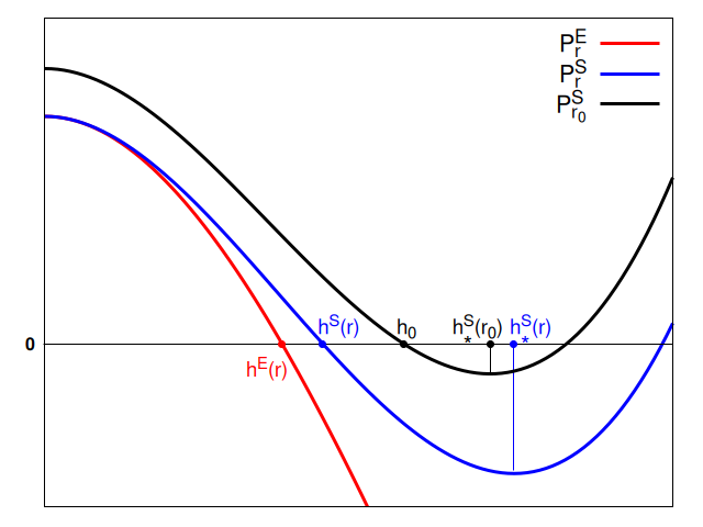
For any fixed $r$, let us denote by $h^{M}(r)$ the water depth solution of the two models, $M\in\{E,S\}$. In what follows, our goal is to obtain an estimation of how large is the influence of $\nu$ on the difference between $h^{S}(r)$ and $h^{E}(r)$. We consider the case of a monotone decreasing surface function $f(r)$ with $f(r_{0})>f(r_{1})$ and a boundary data given at $r=r_{0}$

$$h(r_{0})=h_{0},\quad u(r_{0})=u_{0}.$$ (13)

For the sake of simplicity, we consider that $\nu(r_{0})=1$.

Proposition 1.

If $\displaystyle\frac{u_{0}^{2}}{gh_{0}}>1$ and $f^{\prime}(r)\leq 0$, then:

• the solution $h^{M}(r)$ of ${\cal P}^{M}_{r}(h)=0$ exists for $M\in\{E,S\}$,

• $h^{E}(r)\leq h^{S}(r)$,

• $\exists c>0$ s.t. $h^{S}(r)-h^{E}(r)\leq c\cdot(h^{E}(r))^{2}(1-\nu)$,

• $h^{S}(r)-h^{E}(r)\geq L(r)\cdot(h^{S}(r))^{2}(1-\nu)$, where

  $$L(r)=\frac{1}{3\nu(r)\left(\frac{2\eta(r)}{3g\nu(r)}-h^{Q}(r)\right)}>0,\quad\eta(r):=q_{e}-gf(r),\quad h^{Q}(r):=\frac{q_{w}}{r\sqrt{2\eta(r)}},$$

for all $r\in[r_{0},r_{1}]$.

Proof.

(1) Knowing that

$$\tilde{q}_{e}=q_{e}=\frac{1}{2}u_{0}^{2}+g\left(f(r_{0})+h_{0}\right)$$

holds for $\nu(r_{0})=1$ and denoting

$$\nu^{M}(r):=\left\{\begin{array}[]{lcl}\nu(r),&{\rm if}&M=E\\ 1,&{\rm if}&M=S\end{array}\right.,$$

one observes the following:

• $\displaystyle\partial_{h}{\cal P}^{M}_{r}(h)=3g\nu^{M}(r)h^{2}-2\eta(r)h,$

• $\displaystyle{\cal P}^{M}_{r_{0}}(h_{0})=0,\quad\forall M\in\{E,S\}$,

• $\partial_{r}{\cal P}^{S}_{r}(h)=gf^{\prime}(r)h^{2}-\displaystyle\frac{q_{w}^{2}}{r^{3}}$.

Using properties (a), (b), (c), one can now prove that each of the polynomial equation ${\cal P}^{M}_{r}(h)=0$ has three real roots and since

$$\frac{2\eta(r_{0})}{3g}-h_{0}=\frac{1}{3g}(u_{0}^{2}-gh_{0})>0,$$

one concludes that only one root is a continuous function of $r$ which approaches $h_{0}$ as $r\rightarrow r_{0}$. We call that root the solution of shallow water equation model $M$ and we denote it by $h^{M}(r)$, where $M\in\{E,S\}$.

(2) For each $M\in\{E,S\}$, let us denote by $h_{\star}^{M}(r)$ the nonzero root of the derivative of ${\cal P}_{r}^{M}$ with respect to $h$, i.e.

$$h_{\star}^{M}(r):=\displaystyle\frac{2}{3g}\frac{\eta(r)}{\nu^{M}(r)}.$$

Observing that

$$\begin{array}[]{c}h^{S}_{\star}(r)>h^{S}_{\star}(r_{0})>h_{0},\\ \partial_{r}{\cal P}^{S}_{r}(h)<0,\quad{\cal P}^{E}(h)<{\cal P}^{S}(h),\quad\forall h>0,\end{array}$$

one can immediately conclude that

$$h^{E}(r)<h^{S}(r)<h_{0},\quad r\in(r_{0},r_{1}),$$

see also Fig. 1.

(3) Since

$${\cal P}^{S}(h^{E})={\cal P}^{S}(h^{E})-{\cal P}^{E}(h^{E})=g(1-\nu)(h^{E})^{3}$$

and

$${\cal P}^{S}(h^{E})={\cal P}^{S}(h^{E})-{\cal P}^{S}(h^{S})=({\cal P}^{S})^{\prime}(\xi)(h^{E}-h^{S}),$$

for some $\xi\in(h^{E},h^{S})$, then

$$h^{S}-h^{E}=\displaystyle\frac{(1-\nu)(h^{E})^{3}}{3\xi(h^{S}_{\star}-\xi)}.$$

As $h^{E}<\xi<h^{S}$ and $h^{S}_{\star}(r)-\xi>h^{S}_{\star}(r_{0})-h_{0}$, one can now easily conclude that

$$h^{S}-h^{E}<(1-\nu)(h^{E})^{2}\displaystyle\frac{g}{u_{0}^{2}-gh_{0}}.$$ (14)

(4) Observe that

$$\eta(r)>0,\quad\forall r\in[r_{0},r_{1}],$$

$h^{Q}(r)$ is the positive root of the polynomial

$${\cal Q}_{r}(h):=-\eta(r)h^{2}+\frac{q_{w}^{2}}{2r^{2}},$$ (15)

and that

$${\cal P}_{r}^{S}(h)\geq{\cal P}_{r}^{E}(h)\geq{\cal Q}_{r}(h),\quad\forall h\geq 0.$$ (16)

But ${\cal P}_{r}^{S}(\cdot)$, ${\cal P}_{r}^{E}(\cdot)$, ${\cal Q}_{r}(\cdot)$ are monotone decreasing on $\left[0,\frac{2\eta(r)}{3g}\right]$ and ${\cal Q}_{r}(h^{Q})={\cal P}_{r}^{E}(h^{E})={\cal P}_{r}^{S}(h^{S})=0$; thus (16) now gives

$$0<h^{Q}(r)<h^{E}(r)\leq h^{S}(r)\leq\frac{2\eta(r)}{3g},\quad\forall r\in[r_{0},r_{1}].$$ (17)

Since

$${\cal P}^{E}(h^{S})={\cal P}^{E}(h^{S})-{\cal P}^{S}(h^{S})=g(\nu-1)(h^{S})^{3}$$

and

$${\cal P}^{E}(h^{S})={\cal P}^{E}(h^{S})-{\cal P}^{E}(h^{E})=({\cal P}^{E})^{\prime}(\xi)(h^{S}-h^{E}),$$

for some $\xi\in(h^{E},h^{S})$, then

$$h^{S}-h^{E}=\displaystyle\frac{(1-\nu)(h^{S})^{3}}{3\nu\xi(h^{E}_{\star}-\xi)}.$$ (18)

The “lower bound” inequality from the proposition can now be easily obtained observing that $0<\xi<h^{S}$ and $0<h^{E}_{\star}-\xi<h^{E}_{\star}-h^{Q}$. ∎

Figure 1: Graphical sketch for Proposition 1. The black curve is the graph of the polynomial function ${\cal P}^{E}_{r_{0}}$ which coincides with ${\cal P}^{S}_{r_{0}}$. The red and the blue curves are the graphs of ${\cal P}^{E}_{r}$ and ${\cal P}^{S}_{r}$ for a fixed $r$, respectively.

Remark 1.

If $\nu(r_{0})<1$ then statement (1) will continue to hold, statement (2) may not be true along the entire interval $(r_{0},r_{1})$, and statement (3) must be read as

$$\left|h^{S}(r)-h^{E}(r)\right|\leq c\cdot(h^{E}(r))^{2}(1-\nu).$$

Remark 2.

For the case of monotone increasing profile $f^{\prime}>0$ with boundary data given at $r=r_{1}$ and $\nu(r_{1})=1$, statement (4) continues to hold provided that the solution $h^{S}$ exists for any $r\in(r_{0},r_{1})$. Furthermore, if in addition $h^{S}$ remains upper bounded by $h_{0}$, then statement (3) also continues to hold.

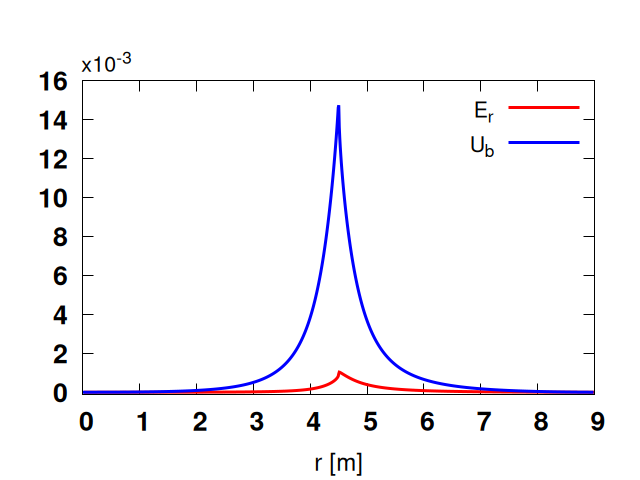
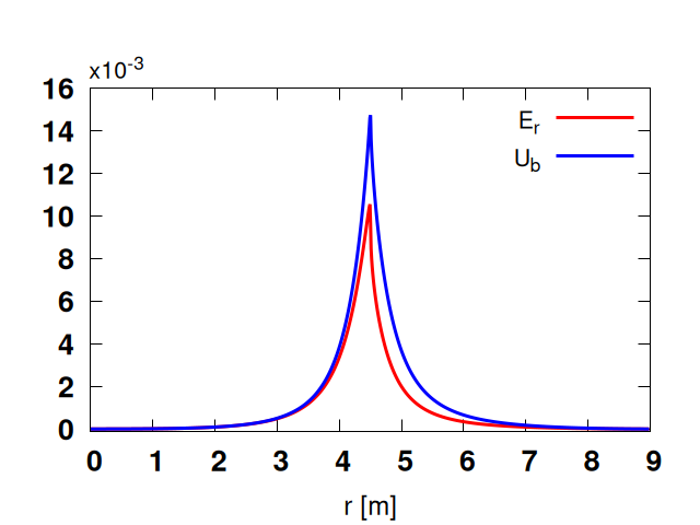
In order to “illustrate” Proposition 1 and the remarks, we consider two particular cases of profiles $f$. Fig. 2 shows the graphs of the relative error $E_{r}:={\left(h^{S}-h^{E}\right)}/{h^{E}}$ and

$$U_{b}:=\frac{h^{E}}{h_{0}}\frac{1-\nu}{Fr^{2}-1}$$ (19)

that can be derived from (14), where $Fr:=u_{0}/{\sqrt{gh_{0}}}$ is the Froude number. For the conditions in Proposition 1, $U_{b}$ is an upper bound for $E_{r}$.

Figure 2: Relative errors between $h^{E}$ and $h^{S}$ for surfaces generated by two different profiles $f$ from Fig. 4. The first column corresponds to a water flow on a type (III) surface, while the second column corresponds to a flow on a type (II) surface. The profile $f$ has $\nu_{0}=1$ on the first row and $\nu_{0}<1$ on the second row.

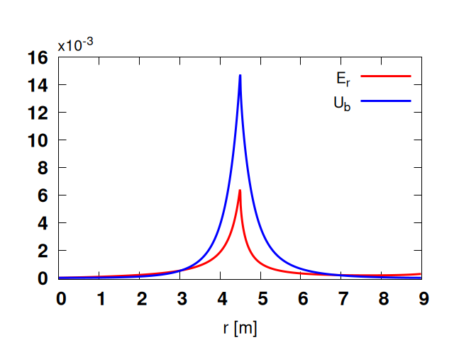Note that the hypotheses of Proposition 1 are fulfilled here only by the flow corresponding to the top left figure.

Remark 3.

The estimation given by statement (3) is mainly important for practical applications where the water depth has small values and it shows that the simplified model S-SWE is still able to reflect the influence of variation in the curvature of the base flow surface on the dynamics of water flow.

Remark 4.

Although the difference between the solutions of the two models is generally small, the estimation given by statement (4) emphasizes that this difference exists and it is not zero.

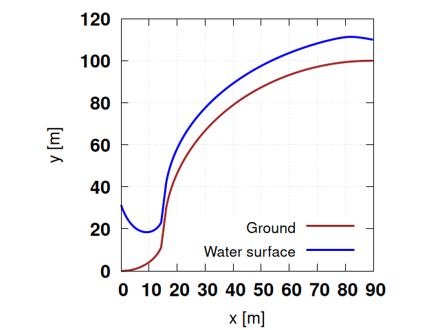
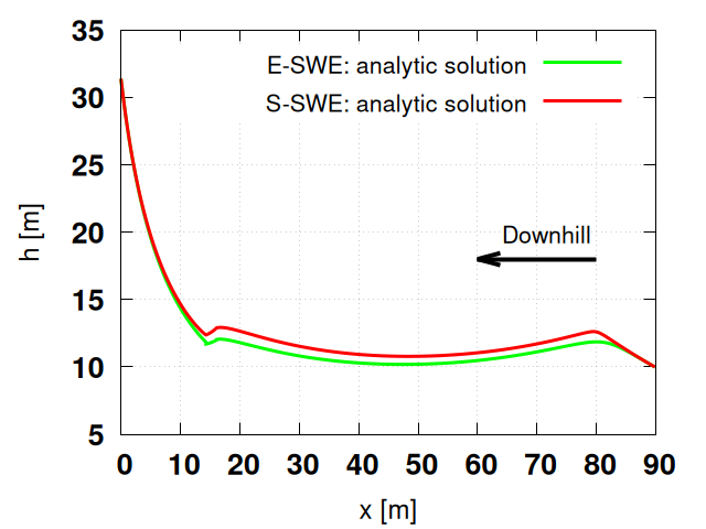
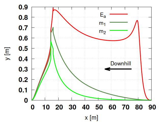
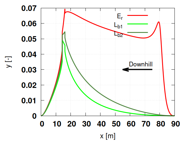
Fig. 3 reflects a particular case where the difference between the two solutions $h^{S}$ and $h^{E}$ is not so neglectable anymore.

Figure 3: The stationary water flow on a radial symmetric surface generated by two quarter circles. The top left picture presents the profile $f$ with $\nu(r_{1})=1$ and the water surface of the steady state flow. The top right picture illustrates the graphics of the water depth corresponding to the solutions of the two models. The absolute and relative errors (between $h^{E}$ and $h^{S}$) and their lower bounds defined in (20) and (21) are pictured on the bottom row.

It shows the graphs of

$$E_{a}:=h^{S}-h^{E},\quad m_{b1}:=L\cdot(h^{S})^{2}(1-\nu),\quad m_{b2}:=L\cdot(h^{Q})^{2}(1-\nu),\quad$$ (20)

$$E_{r}:={\left(h^{S}-h^{E}\right)}/{h^{S}},\quad L_{b1}:=\frac{m_{b1}}{h^{S}},\quad L_{b2}:=\frac{m_{b2}}{h^{Q}}.$$ (21)

that can be derived from the last property of Proposition 1. For the conditions in Proposition 1, $m_{b}$ and $L_{b}$ are lower bounds for the absolute $E_{a}$ and relative $E_{r}$ errors, respectively.

4 Numerical Solutions

For most real life problems, one does not know the analytic solutions of the shallow water models as in [10, 11], and as a consequence, one uses the numerical solutions of S-SWE [2, 4, 12, 13, 14, 15, 16, 17]. The numerical methods developed to solve S-SWE have an intrinsic mathematical interest and they provide solutions for real problems coming from many other areas [18, 19, 20]. Taking this into account, it is relevant (from the application point of view) to compare the numerical solutions of S-SWE with the exact ones of E-SWE.

As we pointed out in the previous sections, it is of main interest to investigate the effects of the curvature variation on the solution of shallow water equation. We noticed that both models give basically the same solutions for a large class of surfaces. However, one can find certain surfaces leading to significant differences between the solutions of the two models.

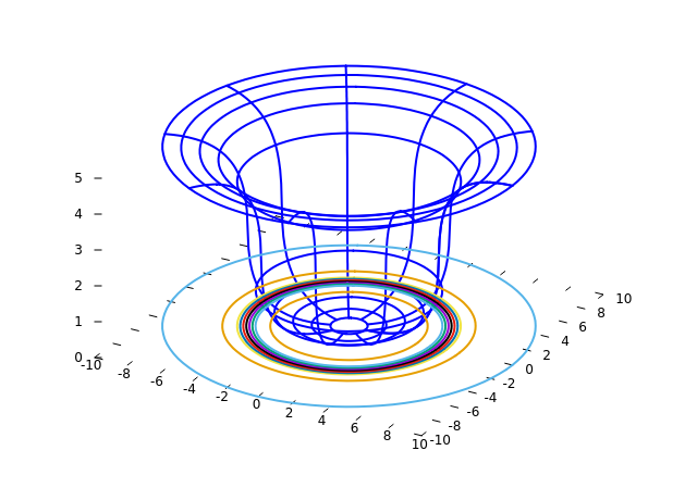
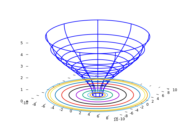
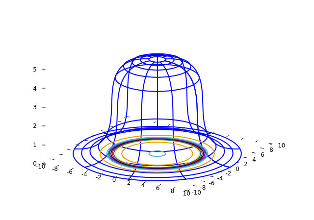
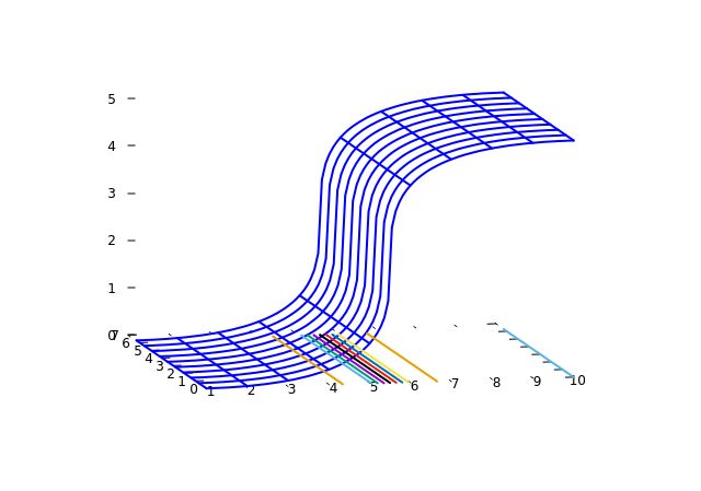
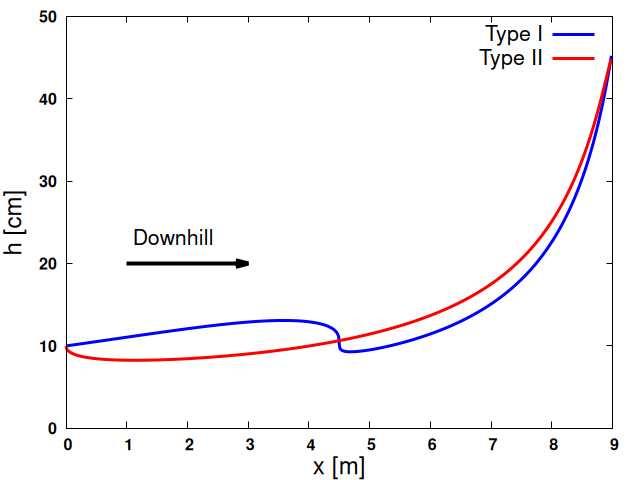
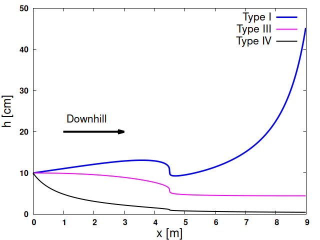
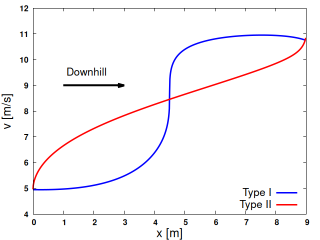
In many applications, especially in hydrological sciences, one considers that the average inclination of the base flow surface is the dominant factor that determines the water dynamics. But in real problems, the surface exhibits local variation of its geometrical properties. To illustrate the influence of such local variation of the surface curvature, we consider four types of surfaces as in Fig. 4, all having the same average slope. Three surfaces have radial symmetry and the fourth one is generated by the translation of a 1D profile.

Crater type (I)	Crater type (II)
Hillock type (III)	Waterfall $1$D type (IV)

Figure 4: Four different types of surfaces $f$. All surfaces have the same height, $5$ m. Surfaces I, III and IV are generated by functions of type $g(\xi)=\sqrt[3]{\xi}-\xi/3$, while surface II is generated by an $\arcsin$ function, applying convenient translations and dilatation of arguments. The three radial symmetric surfaces are defined for $r\in[1,10]$ and the fourth surface for $x\in[1,10]$.

The boundary conditions are the same for all four examples: $h_{0}=0.1$ m and $Fr=5$ at the top of the surface and free drainage the bottom.

The two left pictures of Fig. 5 (built on similar surfaces with the same line curvature with respect to $\theta$) show the influence of the radial curvature on the flow dynamics on crater type surfaces (I and II) where water accumulates at the bottom. We note that the $h$ profiles for both surfaces remain close to each other, while the $v$ profiles have significant differences. The two right pictures of Fig. 5 show the influence of the $\theta$ line curvature on the flow. As opposed to the left, the $v$ profiles for all three types of soil surfaces (I, III and IV) stay close to each other, but there are considerable differences in the $h$ profiles.

Figure 5: Effects of the curvature on the flow distribution along four types of surfaces $f$.

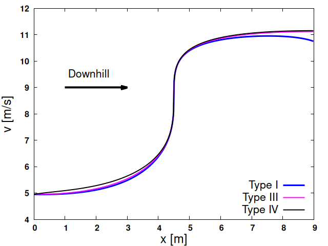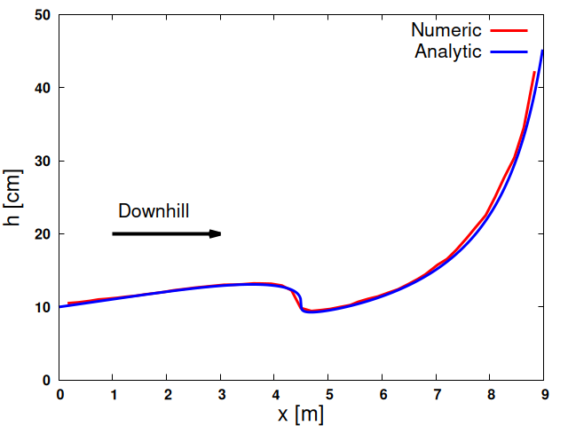
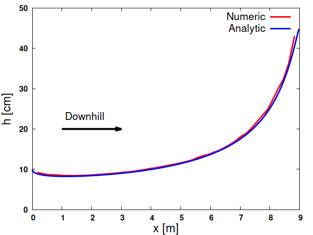
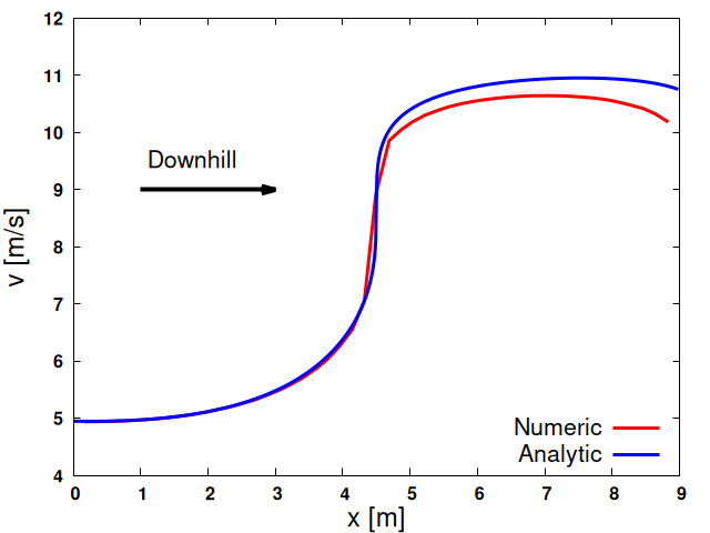
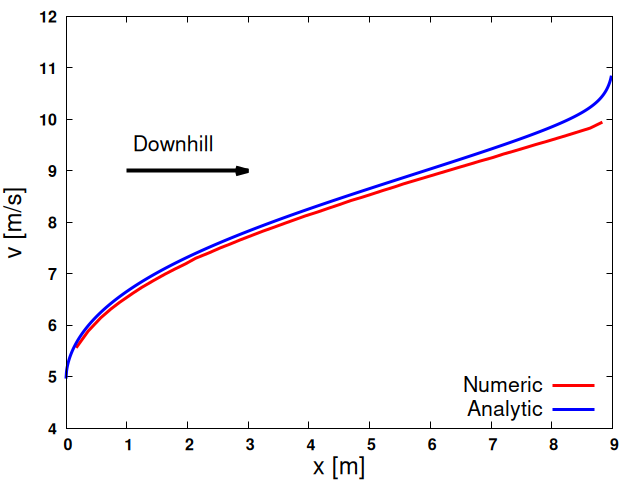
Fig. 6 shows there is a good agreement between the analytic and numerical solutions of the two models for two types of surfaces $f$ (I and II).

Figure 6: Comparison between the analytic solution of E-SWE and the numerical solution of S-SWE for the water flow on surface I (left column) and water flow on surface II (right column).

The numerical solution of S-SWE (1) is obtained by applying the method described in [21]. The finite volume method uses a triangular mesh (obtained by using a quality mesh generator (see [22, 23] for details)) on a 2D domain. In all the applications with radial symmetric surfaces (I, II and III) we consider here, the 2D domain is an annulus

$$D:=\{(r,\theta)\left|\,r\in[r_{0},r_{1}],\,\theta\in[0,2\pi)\right.\}.$$

and the boundary conditions are of Dirichlet type for the upper part and free discharge for the bottom part of the surface:

$$h(t,\boldsymbol{x})=h_{0}=0.1,\quad\boldsymbol{v}(t,\boldsymbol{x})=-v_{0}\boldsymbol{n},\quad\forall\boldsymbol{x}\in\partial D^{\rm in},$$ (22)

where $\partial D^{\rm in}$ is the upper boundary of the surface, $\boldsymbol{n}$ is the external oriented unit normal vector of $\partial D^{\rm in}$ at $\boldsymbol{x}$, and $v_{0}=5\sqrt{0.1g}$.

5 Comments and Conclusions

The E-SWE model can be seen as an intermediate model between the S-SWE model and a mode general model where the hydrostatic approximation of the pressure field is not enforced. The E-SWE model tries to be more realistic by taking into account the variation of the normal direction to the surface. From the analysis presented in this article, we can conjecture that for a moderate variation of the surface curvature, the gradient of the surface is sufficient to find solutions that catch the variation of surface curvature, see Fig. 5.

We can also make a remark concerning the physical signification of the shallow water S-SWE model: the good agreement between the solutions of the two models (see Fig. 2 and the remarks from Section 3) suggest us to think the velocity $\boldsymbol{v}$ of the S-SWE model as vector in the tangent plane to the surface and $h$ as water depth in the normal direction to the surface.

Finally, note that for an adequate utilization of the S-SWE model in real life problems, one must specify a proper reference surface for the variables.

References

- [1] F. Bouchut, Nonlinear Stability of Finite Volume Methods for Hyperbolic Conservation Laws and Well-Balanced Schemes for Sources, Frontiers in Mathematics, Birkhäuser Verlag, Basel, 2004.
- [2] L. Cozzolino, V. Pepe, L. Cimorelli, A. D’Aniello, R. D. Morte, D. Pianese, The solution of the dam-break problem in the porous shallow water equations, Advances in Water Resources 114 (2018) 83–101. doi:10.1016/j.advwatres.2018.01.026.
- [3] J. C. I. Dooge, A general theory of the unit hydrograph, Journal of Geophysical Research 64 (2) (1959) 241–256. doi:10.1029/JZ064i002p00241.
- [4] T.-W. Hsu, S.-J. Liang, N.-J. Wu, Application of meshless swe model to moving wet/dry front problems, Engineering with Computers 35 (1) (2019) 291–303. doi:10.1007/s00366-018-0599-1.
- [5] S. Ion, D. Marinescu, S.-G. Cruceanu, Fluid flow on vegetated hillslope, arXiv (2020) 1–27doi:10.48550/ARXIV.2006.14367.
- [6] R. F. Dressler, New nonlinear shallow-flow equations with curvature, Journal of Hydraulic Research 16 (3) (1978) 205–222. doi:10.1080/00221687809499617.
- [7] B. Dewals, S. Erpicum, P. Archambeau, S. Detrembleur, M. Pirotton, Depth-integrated flow modelling taking into account bottom curvature, Journal of Hydraulic Research 44 (6) (2006) 785–795. doi:10.1080/00221686.2006.9521729.
- [8] Y. T. Zerihun, Modelling free surface flow with curvilinear streamlines by a non-hydrostatic model, Journal of Hydrology and Hydromechanics 64 (3) (2016) 281–288. doi:doi:10.1515/johh-2016-0028.
- [9] R. Berger, G. Carey, Free-surface flow over curved surfaces: Part i: Perturbation analysis, International Journal for Numerical Methods in Fluids 28 (1998) 191–200. doi:10.1002/(SICI)1097-0363(19980815)28:2¡357::AID-FLD750¿3.0.CO;2-D.
- [10] O. Delestre, C. Lucas, P.-A. Ksinant, F. Darboux, C. Laguerre, et al., SWASHES: a compilation of shallow water analyticsolutions for hydraulic and environmental studies, International Journal for Numerical Methods in Fluids 72 (3) (2013) 269–300. doi:10.1002/fld.3741.
- [11] N. Matskevich, L. Chubarov, Exact solutions to shallow water equations for a water oscillation problem in an idealized basin and their use in verifying some numerical algorithms, Numerical Analysis and Applications 12 (2019) 234–250. doi:10.1134/S1995423919030030.
- [12] S. F. Bradford, B. Sanders, Finite-volume model for shallow-water flooding of arbitrary topography, Journal of Hydraulic Engineering 128 (3) (2002) 289–298. doi:10.1061/(ASCE)0733-9429(2002)128:3(289).
- [13] A. Chinnayya, A. Y. LeRoux, N. Seguin, A well-balanced numerical scheme for the approximation of the shallow-water equations with topography: the resonance phenomenon, International Journal on Finite Volumes 1 (2004) 1–33.
- [14] F. Benkhaldoun, M. Seaid, A simple finite volume method for shallow water equation, Journal of Computational and Applied Mathematics 234 (2010) 58–72. doi:10.1016/j.cam.2009.12.005.
- [15] U. S. Fjordholm, S. Mishra, E. Tadmor, Well-balanced and energy stable schemes for the shallow water equations with discontinuous topography, Journal of Computational Physics 230 (14) (2011) 5587–5609. doi:10.1016/j.jcp.2011.03.042.
- [16] Y. Liu, J. Zhou, L. Song, Q. Zou, L. Liao, Y. Wang, Numerical modelling of free-surface shallow flows over irregular topography with complex geometry, Applied Mathematical Modelling 37 (2013) 9482–9498. doi:10.1016/j.apm.2013.05.001.
- [17] F. Marche, P. Bonneton, P. Fabrie, N. Seguin, Evaluation of well-balanced bore-capturing schemes for 2d wetting and drying processes, International Journal for Numerical Methods in Fluids 53 (2007) 867–894. doi:10.1002/fld.1311.
- [18] V. Iordache, A. Neagoe, Conceptual methodological framework for the resilience of biogeochemical services to heavy metals stress, Journal of Environmental Management 325 (2022) 116401. doi:10.1016/j.jenvman.2022.116401.
- [19] P. García-Navarro, J. Murillo, J. Fernández-Pato, I. Echeverribar, M. Morales-Hernández, The shallow water equations and their application to realistic cases, Environmental Fluid Mechanics 19 (2019) 1235–1252. doi:10.1007/s10652-018-09657-7.
- [20] D. Bresch, Chapter 1 - shallow-water equations and related topics, in: C. Dafermos, M. Pokorný (Eds.), Handbook of Differential Equations, Vol. 5 of Handbook of Differential Equations: Evolutionary Equations, North-Holland, 2009, pp. 1–104. doi:10.1016/S1874-5717(08)00208-9.
- [21] S. Ion, D. Marinescu, S.-G. Cruceanu, Numerical scheme for solving a porous saint-venant type model for water flow on vegetated hillslopes, Applied Numerical Mathematics 172 (2022) 67–98. doi:10.1016/j.apnum.2021.09.019.
- [22] J. R. Shewchuk, Triangle: Engineering a 2D Quality Mesh Generator and Delaunay Triangulator, in: M. C. Lin, D. Manocha (Eds.), Applied Computational Geometry: Towards Geometric Engineering, Vol. 1148 of Lecture Notes in Computer Science, Springer-Verlag, 1996, pp. 203–222, from the First ACM Workshop on Applied Computational Geometry.
- [23] J. R. Shewchuk, Delaunay refinement algorithms for triangular mesh generation, Computational Geometry 22 (2002) 21–74. doi:10.1016/S0925-7721(01)00047-5.