A Simple Zero-shot Prompt Weighting Technique to Improve Prompt Ensembling in Text-Image Models

Abstract

Contrastively trained text-image models have the remarkable ability to perform zero-shot classification, that is, classifying previously unseen images into categories that the model has never been explicitly trained to identify. However, these zero-shot classifiers need prompt engineering to achieve high accuracy. Prompt engineering typically requires hand-crafting a set of prompts for individual downstream tasks. In this work, we aim to automate this prompt engineering and improve zero-shot accuracy through prompt ensembling. In particular, we ask “Given a large pool of prompts, can we automatically score the prompts and ensemble those that are most suitable for a particular downstream dataset, without needing access to labeled validation data?”. We demonstrate that this is possible. In doing so, we identify several pathologies in a naive prompt scoring method where the score can be easily overconfident due to biases in pre-training and test data, and we propose a novel prompt scoring method that corrects for the biases. Using our proposed scoring method to create a weighted average prompt ensemble, our method outperforms an equal average ensemble, as well as hand-crafted prompts, on ImageNet, 4 of its variants, and 11 fine-grained classification benchmarks, all while being fully automatic, optimization-free, and not requiring access to labeled validation data.

1 Introduction

Figure 1: Construction of a zero-shot classifier with zero-shot prompt ensembling (ZPE) for text-image models. Logits (* □) are calculated by combining text (* □) and image (* □) representations. The final text representation is a weighted ensemble of representations corresponding to different prompts (* □). Crucially, the ZPE scores (* □) for weighting each prompt are calculated without access to any labeled training data, as described in Sections 3 and 2.

Contrastively trained text-image models such as CLIP (Radford et al., 2021), ALIGN (Jia et al., 2021), LiT (Zhai et al., 2022), and BASIC (Pham et al., 2021) have the remarkable ability to perform zero-shot classification. That is, such models can be used to classify previously unseen images into categories for which the model has never been explicitly trained to identify. Such zero-shot classifiers can match the performance of standard classification models which have access to training examples. For example, a CLIP zero-shot classifier with a ViT-L/14 vision tower matches the ImageNet accuracy of a ResNet-101 (Radford et al., 2021). However, achieving strong zero-shot classification performance requires prompt engineering (Radford et al., 2021; Zhai et al., 2022; Pham et al., 2021). Zero-shot CLIP ViT-B/16 performance on ImageNet increases from 64.18% to 66.92% and 68.57% when using the prompt ‘A photo of {}.’, and a selection of 80 hand-crafted prompts, rather than class name only. To use a set of hand-crafted prompts for zero-shot classification, the text embeddings of the prompts composed with class names are averaged into a single vector to represent the class. This is called a prompt ensemble in (Radford et al., 2021). Prompt engineering can be seen as reducing the ‘distribution shift’ between the zero-shot setting and the training data in which the captions seldom consist of a single word.

Unfortunately, the need for a set of hand-crafted prompts to achieve good zero-shot performance greatly reduces the promised general applicability of such zero-shot classifiers. Different sets of prompts were manually designed and tuned for different downstream tasks for CLIP. For example, the prompts ‘a photo of a {} texture.’, ‘a photo of a {} pattern.’, and ‘i love my {}!’, ‘a photo of my clean {}.’ were designed for the Describable Textures Dataset (DTD) (Cimpoi et al., 2014) and the Cars196 dataset (Krause et al., 2013) , respectively. Designing different sets of hand-crafted prompts can be be labor-intensive, and the common prompt design processes require access to a labeled validation dataset, which may not be available in practice. In this paper, we ask the question “Can we automate prompt engineering for zero-shot classifiers?”. Specifically, given a zero-shot model and a large pool of potential prompts, our goal is to select the optimal subset of prompts that maximize the model performance in a zero-shot fashion, i.e., without access to a labeled validation set.

Our contributions are the following:

1. We present an algorithm for automatically scoring the importance of prompts in a large pool given a specific downstream task when using text-image models for zero-shot classification. We then propose a weighted average prompt ensembling method using the scores as the weights.

2. We identify several pathologies in a naive prompt scoring method where the score can be easily overconfident due to biases in both pre-training and test data. We address these pathologies via bias correction in a zero-shot and optimization-free fashion.

3. We demonstrate that our algorithm is better performing than the existing approach of hand-crafted prompts, without the need for a labeled validation set and a labor-intensive manual tuning process.

2 Background

We consider contrastively trained text-image models consisting of a text encoder $T$ and an image encoder $I$. The encoders produce embeddings $\mathbf{z}_{\text{txt}}=T(\mathtt{text})$ and $\mathbf{z}_{\text{img}}=I(\mathtt{image})$, both of size $D$.

Training.

The models are trained on batches of $B$ text-image pairs $\{(\mathtt{text}_{b},\mathtt{image}_{b})\}_{b=1}^{B}$—e.g., photographs and their captions—to encourage that $\mathbf{z}_{\text{txt}}^{i}=\mathbf{z}_{\text{img}}^{j}$, if $i=j$, and $\mathbf{z}_{\text{txt}}^{i}\neq\mathbf{z}_{\text{img}}^{j}$ otherwise. This is accomplished with a bi-directional contrastive loss:

$$\mathtt{logits} =\begin{bmatrix}\mathbf{z}_{\text{img}}^{1}\cdot\mathbf{z}_{\text{txt}}^{1}&\mathbf{z}_{\text{img}}^{1}\cdot\mathbf{z}_{\text{txt}}^{2}&\dots&\mathbf{z}_{\text{img}}^{1}\cdot\mathbf{z}_{\text{txt}}^{B}\\ \mathbf{z}_{\text{img}}^{2}\cdot\mathbf{z}_{\text{txt}}^{1}&\mathbf{z}_{\text{img}}^{2}\cdot\mathbf{z}_{\text{txt}}^{2}&\dots&\mathbf{z}_{\text{img}}^{2}\cdot\mathbf{z}_{\text{txt}}^{B}\\ \vdots&\vdots&\ddots&\vdots\\ \mathbf{z}_{\text{img}}^{B}\cdot\mathbf{z}_{\text{txt}}^{1}&\mathbf{z}_{\text{img}}^{B}\cdot\mathbf{z}_{\text{txt}}^{2}&\dots&\mathbf{z}_{\text{img}}^{B}\cdot\mathbf{z}_{\text{txt}}^{B}\end{bmatrix}$$

$$\mathcal{L}_{\text{img}} =-\frac{1}{B}\sum_{b=1}^{B}\log\mathrm{softmax}(\mathtt{logits})_{b,b}$$

$$\mathcal{L}_{\text{txt}} =-\frac{1}{B}\sum_{b=1}^{B}\log\mathrm{softmax}(\mathtt{logits}^{\intercal})_{b,b}$$

$$\mathcal{L} =\left(\mathcal{L}_{\text{img}}+\mathcal{L}_{\text{txt}}\right)/2,$$

which can be interpreted as the average cross-entropy loss when classifying which caption in the batch corresponds to a given image and vice-versa.

Zero-shot prediction.

Once the text and image encoders have been trained, we can setup a zero-shot classifier with $C$ classes for an image with representation $\mathbf{z}_{\text{img}}$ by computing

$$\mathtt{logits} =\begin{bmatrix}\mathbf{z}_{\text{img}}\cdot\mathbf{z}_{\text{txt}}^{1}&\dots&\mathbf{z}_{\text{img}}\cdot\mathbf{z}_{\text{txt}}^{c}&\dots&\mathbf{z}_{\text{img}}\cdot\mathbf{z}_{\text{txt}}^{C}\end{bmatrix}$$

$$\hat{c} =\mathrm{argmax}_{c}\ \mathtt{logits},$$

where $\hat{c}$ is the predicted class, and $\mathbf{z}_{\text{txt}}^{c}=T(\mathtt{class\_name}_{c})$ with $\mathtt{class\_name}$ being a list of possible classes. In the case where we have $P$ prompt templates, prompt ensembling as proposed in (Radford et al., 2021) generalizes the above to

$$\mathtt{logits} =\begin{bmatrix}\mathbf{z}_{\text{img}}\cdot\mathbf{z}_{\text{txt}}^{1,1}&\mathbf{z}_{\text{img}}\cdot\mathbf{z}_{\text{txt}}^{1,2}&\dots&\mathbf{z}_{\text{img}}\cdot\mathbf{z}_{\text{txt}}^{1,C}\\ \mathbf{z}_{\text{img}}\cdot\mathbf{z}_{\text{txt}}^{2,1}&\mathbf{z}_{\text{img}}\cdot\mathbf{z}_{\text{txt}}^{2,2}&\dots&\mathbf{z}_{\text{img}}\cdot\mathbf{z}_{\text{txt}}^{2,C}\\ \vdots&\vdots&\ddots&\vdots\\ \mathbf{z}_{\text{img}}\cdot\mathbf{z}_{\text{txt}}^{P,1}&\mathbf{z}_{\text{img}}\cdot\mathbf{z}_{\text{txt}}^{P,2}&\dots&\mathbf{z}_{\text{img}}\cdot\mathbf{z}_{\text{txt}}^{P,C}\end{bmatrix}$$ (1)

$$\hat{c} =\mathrm{argmax}_{c}\ \frac{1}{P}\sum_{p=1}^{P}\mathtt{logits}_{p}\,,$$ (2)

where $\mathtt{logits}_{p}$ is the $p^{\mathrm{th}}$ row of $\mathtt{logits}$, and $\mathbf{z}_{\text{txt}}^{p,c}=T(\mathtt{prompt\_template}_{p}\circ\mathtt{class\_name}_{c})$, with $\circ$ indicating the composition of a prompt template and a class name, e.g., ‘A photo of a $\{\}$.’ $\circ$ ‘dog’ $=$ ‘A photo of a dog.’. Note that Equation 2 can be seen as constructing an ensemble of classifiers in logit space, where each classifier uses a different prompt.

3 Zero-shot weighted prompt ensembling

In this section, we describe our proposed method: Zero-shot Prompt Ensembling (ZPE) for zero-shot classification with text-image models. Given a large pool of $P$ prompts, which may or may not be entirely relevant to a specific problem at hand, and a previously unseen classification task, we would like to learn a set of scores $\{s_{1},s_{2},\dots,s_{P}\}$ that will allow us to perform a weighted average by replacing Equation 2 with

$$\hat{c} =\mathrm{argmax}\ \frac{1}{P}\sum_{p=1}^{P}\mathtt{logits}_{p}\mathbin{\color[rgb]{0,1,0}\times}{\color[rgb]{0,1,0}s_{p}},$$ (3)

or a masked average by replacing Equation 2 with

$$\hat{c} =\mathrm{argmax}\ \frac{1}{P}\sum_{p=1}^{P}\mathtt{logits}_{p}\mathbin{\color[rgb]{0,1,0}\times}{\color[rgb]{0,1,0}s_{p}\times\mathds{1}(s_{p}>\tau)},$$ (4)

where $\mathds{1}(\cdot)$ is the indicator function. The masked average introduces a hyperparameter $\tau$, the score threshold for prompt subset selection. Thus, we also consider the hyperparameter-free weighted average. The weighted averaging of logits can be regarded as the weighted ensemble of many classifiers, where each of them is made of a different prompt, and the weights are computed in a zero-shot fashion without any optimization or the access to test labels.

3.1 A simple baseline – max logit scoring

The maximum logit over the classes $\mathtt{max\_logit}=\mathrm{max}_{c}\ \mathtt{logits}$ is a commonly used confidence score for classification problems. Since $\mathbf{z}_{\text{img}}$ and $\mathbf{z}_{\text{txt}}$ are $L_{2}$ normalized, i.e. $\|\mathbf{z}_{\text{img}}\|=\|\mathbf{z}_{\text{txt}}\|=1$, the inner product equals to the $L_{2}$ distance up to a constant and a scalar, i.e., $\|\mathbf{z}_{\text{img}}-\mathbf{z}_{\text{txt}}\|^{2}=2-2*\mathbf{z}_{\text{img}}\cdot{\mathbf{z}_{\text{txt}}}^{\intercal}$. Thus, the maximum logit over the classes is equivalent to the minimum $L_{2}$ distance over the classes. The minimum distance is a natural measure of confidence for a prediction. For example, the classic $k$-means algorithm uses it as a measure for clustering (MacQueen, 1967). Recent work also has shown that the maximum logit outperforms the maximum softmax in terms of capturing the uncertainty in prediction (Hendrycks et al., 2019), and it was used as a confidence score in zero-shot classification with text-image models (Ge et al., 2022).

For the problem of prompt scoring, intuitively, if a prompt has large maximum logit values given a set of images, it suggests that the zero-shot classifier is more confident in the predictions, and therefore it is more likely that the prompt is suitable for the image classification task. Thus, we consider Algorithm 1 for using the maximum logit (averaged over images) for scoring prompts.

Algorithm 1 Max Logit Scoring

1:  Input: Image embeddings $\mathbf{Z}_{\text{img}}$ (shape $N\times D$), class embeddings for the $p^{\text{th}}$ prompt $\mathbf{Z}_{\text{txt}}$ (shape $C\times D$).

2:  $\mathtt{logits}=\mathbf{Z}_{\text{img}}\cdot{\mathbf{Z}_{\text{txt}}}^{\intercal}$ # shape: $N\times C$.

3:  $\mathtt{max\_logits}=\mathrm{max}_{c}\ \mathtt{logits}$ # shape: $N$.

4:  $s_{p}=\frac{1}{N}\sum_{n=1}^{N}\mathtt{max\_logits}_{n}$

5:  Output: $s_{p}$, the score for the $p^{\text{th}}$ prompt.

Unfortunately, while this scoring method does work to some extent, it is biased. The biases can easily be seen by looking at the top 10 prompts for ImageNet and Sun397:

We see that some prompts—i.e., those containing the word ‘person’—are scored highly even though the these prompts are not related to the classes of either dataset. By considering the contrastive training of our model we can identify two pathologies that might cause this problem. Prompts are biased towards large logits due to

• Word frequency bias in pre-training data: Prompts containing words, or words with similar semantic meanings to those, that appear more frequently in the pre-training data, and

• Spurious concept frequency bias in test data: Prompts containing frequent words that map to common concepts in the test images, but that are different to the classes of interest for prediction. For example, images in Sun397 often contain people but the classes are various in- and outdoor locations; see Figure 2.

This suggests that the raw max logit score is not trustworthy because the value can be overconfident due to the biases.

(a) Topiary

(b) Bowling alley

(c) Medina

Figure 2: Images from Sun397. Note that the pictures contain the spurious ‘person’ concept which is different from the classes.

3.2 Tackling frequency biases via logit normalization

To correct for these frequency biases, we consider normalizing the raw max logits score by subtracting the expected value under a reference distribution. We use subtraction rather than division for normalization because we are working in log (odds) space. This approach is inspired by the classical likelihood ratio method which compares how different the likelihood evaluated at the observed data is from that evaluated at a reference data (Casella & Berger, 2021; King, 1989), and it is a commonly used technique for reducing biases. For example, the Term Frequency–Inverse Document Frequency (TF-IDF) in information retrieval (Jones, 1972), the likelihood-ratio method and relative Mahalanobis distance method for out-of-distribution detection (Ren et al., 2019, 2021, 2022), and the ratio of observed to expected mortality rate (O/E) in medical studies (Best & Cowper, 1994; Galvan-Turner et al., 2015) all use the expectation as a reference to normalize the raw scores. See Section 5 for further discussion.

Given a pair of a test image and a prompt, we compare the maximum logit for the pair $\mathtt{logits}(\mathtt{test\_img},\mathtt{prompt})$ with the expected maximum logit for a random image with the same prompt $\mathtt{logits}(\mathtt{random\_img},\mathtt{prompt})$. If the prompt contains frequent words in the pre-training data or words that map to unrelated but common concepts in the test data and result in large logits regardless of the content of an image, the expected maximum logit value would be large too. Therefore only when the difference $\mathtt{logits}(\mathtt{img},\mathtt{prompt})-\mathtt{logits}(\mathtt{random\_img},\mathtt{prompt})$ is large, the prompt is considered suitable to the classification task of the test image.

We solve word frequency bias by normalizing the logits for each prompt by subtracting the expected logits based on images in the pre-training data $E_{\text{pretrain}}=\mathbb{E}_{\mathtt{img}\sim\mathcal{D}_{\text{pretrain}}}\left[\mathbf{z}_{\text{img}}\cdot\mathbf{z}_{\text{txt}}\right]$. We estimate the expected logits using the average logits for a wide range of random images sampled from the pre-training data. Since the pre-training data of CLIP is not publicly available, we instead use LAION400m (Schuhmann et al., 2021), since it has been shown that the models pre-trained using LAION dataset could reproduce CLIP models’ performance (Cherti et al., 2022). By removing $E_{\text{pre-train}}$, we down-weigh prompts that contain the frequent words in the pre-training data which would result in large logits regardless of the content of an image. In the experiments, we use a small subsample of LAION400m, i.e., the first 20k images, as we found it is already sufficient to achieve high performance.

As a sanity check, we verify that subtracting $E_{\text{pretrain}}$ from the logits reduces the word frequency bias. We compare the correlation coefficient for the frequency of each word in LAION400m and the average logit $\mathtt{avg\_logit}=\mathbb{E}_{\mathtt{img}\sim\mathcal{D}_{\text{ImagNet}}}\left[\mathbf{z}_{\text{img}}\cdot\mathbf{z}_{\text{word}}\right]$ with the correlation between the word frequency and $\mathtt{avg\_logit}-E_{\text{pretrain}}$. Without normalisation we have a Pearson correlation coefficient of 0.09 with a p-value of $3.6\times 10^{-11}$. With normalisation we have a correlation coefficient of -0.03 with a p-value of 0.03. That is, subtracting $E_{\text{pretrain}}$ removes the statistically significant correlation between logit magnitude and word frequency.

We solve spurious concept frequency bias subtracting the expected logits for the images in the test data itself $E_{\text{test}}=\mathbb{E}_{\mathtt{img}\sim\mathcal{D}_{\text{test}}}\left[\mathbf{z}_{\text{img}}\cdot\mathbf{z}_{\text{txt}}\right]$. Our intuition is that if there are spurious but common concepts shared among test images, averaging the logits would provide a good reference of the maximum logit value for an general image containing the concepts. By removing $E_{\text{test}}$, we down-weigh prompts that contain words that map to common but spurious concepts.

To jointly reduce the both types of biases, we average over $E_{\text{pretrain}}$ and $E_{\text{test}}$. In summary, Algorithm 2 shows our method for scoring prompts with normalization.

Algorithm 2 Normalized Max Logit Scoring

1:  Input: Image embeddings $\mathbf{Z}_{\text{img}}$ (shape $N\times D$), class embeddings for the $p^{\text{th}}$ prompt $\mathbf{Z}_{\text{txt}}$ (shape $C\times D$), embeddings of pre-train images $\mathbf{Z}_{\text{pretrain}}$ (shape $N^{\prime}\times D$).

2:  $\mathtt{logits}=\mathbf{Z}_{\text{img}}\cdot{\mathbf{Z}_{\text{txt}}}^{\intercal}$ # shape: $N\times C$.

3:  $\mathtt{logits_{\text{pretrain}}}=\mathbf{Z}_{\text{pretrain}}\cdot{\mathbf{Z}_{\text{txt}}}^{\intercal}$ # shape: $N^{\prime}\times C$.

4:  $E_{\text{pretrain}}=\frac{1}{N^{\prime}}\sum_{n=1}^{N^{\prime}}\mathtt{logits_{\text{pretrain,n}}}$

5:  $E_{\text{test}}=\frac{1}{N}\sum_{n=1}^{N}\mathtt{logits}_{n}$

6:  $\mathtt{logits_{\text{normalized}}}=\mathtt{logits}-(E_{\text{pretrain}}+E_{\text{test}})/2$

7:  $\mathtt{max\_logits}=\mathrm{max}_{c}\ \mathtt{logits}_{{\color[rgb]{0,1,0}\text{normalized}}}$ # shape: $N$.

8:  $s_{p}=\frac{1}{N}\sum_{n=1}^{N}\mathtt{max\_logits}_{n}$

9:  Output: $s_{p}$, the score for the $p^{\text{th}}$ prompt.

3.3 Handling long-tails via softmax weighting

When scoring a large number of prompts, we observe a long tail behaviour, where a small number of prompts have large scores, but most prompts are “bad” and have small scores. Despite receiving small scores, the irrelevant prompts can still collectively provide a large impact on the weighted average in Equation 3. To mitigate this issue, we replace Equation 3 with

$$\vspace{-0.75em}\mathtt{c}\vspace{-0.2em} =\vspace{-0.2em}\mathrm{argmax}\ \!\frac{1}{P}\!\sum_{p=1}^{P}\mathtt{logits}_{p}\times{\color[rgb]{0,1,0}\mathrm{softmax}(}s{\color[rgb]{0,1,0})}_{p}.\vspace{-0.4em}$$ (5)

The softmax function is applied over the prompt sets such that the weights are summed to 1. Figure 3 shows the impact of (i) the long tail of low ZPE scores on weighted prompt ensemble ImageNet accuracy, and (ii) the reduced impact when using softmax weighting. Note that without softmax weighting, adding additional prompts has a large negative effect on accuracy once irrelevant prompts start to be included in the ensemble.

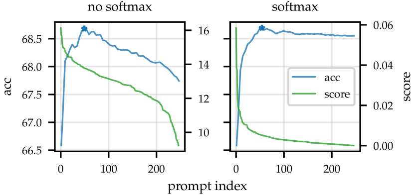
Figure 3: CLIP ViT-B/16 ImageNet accuracy (given a weighted ensemble of all prompts up to the prompt index on the x-axis) and the ZPE scores corresponding to each prompt, with and without softmax weighting.

3.4 Prompt selection

So far we have considered principled normalization techniques for countering the frequency biases in pre-training and test data and the long-tail issue in computing prompt scores $s_{p}$ for the weighted ensemble (3). For computing the masked ensemble (4), we also need to set the score threshold parameter $\tau$. Here, we consider prompt selection as an outlier detection problem. We assume that in a large pool of prompts, the majority of the prompts are irrelevant to a specific downstream dataset. Thus, the relevant prompts can be regarded as outliers to the pool distribution. We use the median absolute deviation (Rousseeuw & Croux, 1993) test statistic which is similar to using a $z$-test statistic, but is more robust to extreme events and non-Gaussian distributions. Concretely, we calculate the median $\bar{s}=\mathrm{median}_{p}\left(s\right)$ and median absolute deviation $\tilde{d}=\mathrm{median}_{p}\left(|s-\bar{s}|\right)$. We then compute the $z$-score for given a prompt,

$$z =\frac{s-\bar{s}}{\tilde{d}}.$$

We classify the $p^{\text{th}}$ prompt as an outlier if $z_{p}>\tau$. Here, $\tau$ is analogous to a desired standard deviation in a $z$-test. The advantage of this approach, rather than thresholding the scores directly, is that we can set $\tau$ without knowledge of the magnitudes of the scores. This allows us to use the same value of $\tau$ for multiple datasets.

4 Experimental Evaluation

To evaluate the quality of our prompt scores, we compare our zero-shot prompt ensembling (ZPE) method, to a number of baselines. We also perform various ablation and sensitivity studies. Unless otherwise specified, we use score normalization, and softmax weighting. We evaluate the methods on ImageNet (Russakovsky et al., 2015), and its variant test sets ImageNet-R, ImageNet-A, ImageNet-Sketch, and ImageNet-V2 (Hendrycks et al., 2021a, b; Wang et al., 2019; Recht et al., 2019). We also evaluate on Caltech101, Cars196, CIFAR10, CIFAR100, DTD, EuroSat, Food-101, Oxford flowers, Oxford pets, Resisc45, and Sun397 which are fine-grained classification datasets covering several different domains; see Section B.1 for more details.

Note that our CLIP results (e.g., rows 1-3 in Tables 1 and 2) differ from those presented by Radford et al. (2021). This is due to two factors. Firstly, in several cases—e.g., for the Caltech101 dataset—Radford et al. (2021) did not specify the dataset split they used. Thus we had to make guesses which do not necessarily agree with their choices; see Section B.1 for our splits. Secondly, we found that the implementation of resize in tensorflow_datasets, which we used for data pre-processing, differs slightly from the torchvision implementation used by Radford et al. (2021). This implementation difference caused large differences in performance for some datasets.

4.1 Creating a pool of prompts

Ideally, we would like to have a varied pool of thousands of hand-crafted prompts. Such a set of prompts would contain a range of generic prompts—such as ‘A photo of {}.’ and ‘An example of {}.’—that would be useful for a many classification tasks, as well as more specific prompts—such as ‘A photo of {}, a type of flower.’ and ‘A cartoon of {}.’—that we expect to be useful for a smaller range of tasks. Unfortunately, no such set of prompts exists.

In the following experiments, we simulate such a pool by combining the 27 sets of prompts designed by Radford et al. (2021) and the prompts designed for 14 datasets by Zhai et al. (2022). This leaves us with a pool of 247 unique prompts. See Appendix D for details. In section A.1 we use the large language model, ChatGPT (OpenAI, 2022), to generate 179 additional prompt templates, resulting in a pool of 426 total templates. We then use that to study the impact of the size of the pool set on performance.

4.2 ZPE weighted average

Table 1: Zero-shot accuracy on ImageNet and its variants. ZPE is applied to the pool set. Note that the hand-crafted prompt sets were highly optimised and manually tuned on labeled validation sets, while our method ZPE is automatic and cheap to compute.

	ImageNet	ImageNet-A	ImageNet-R	ImageNet-Sketch	ImageNet-V2	Avg
CLIP ViT-B/16
class name	63.94	46.01	74.92	44.12	57.97	57.39
‘A photo of {}.’	66.37	47.47	73.78	45.84	60.46	58.78
hand-crafted, equal average	68.31	49.13	77.31	47.65	61.83	60.85
pool set, equal average	67.59	49.35	77.33	46.92	61.37	60.51
max-logit scoring	67.63	49.37	77.38	46.95	61.39	60.55
ZPE (weighted average)	68.56	49.61	77.69	47.92	62.23	61.20
ZPE (prompt selection, ours)	68.60	49.63	77.62	47.99	62.21	61.21
LiT ViT-L/16
class name	78.26	62.36	89.80	64.24	71.61	73.26
‘A photo of {}.’	78.22	62.43	89.45	63.73	71.35	73.03
hand-crafted, equal average	78.55	63.09	90.52	64.90	72.10	73.83
pool set, equal average	77.49	62.07	90.25	63.49	71.17	72.89
max-logit scoring	77.86	62.31	90.47	63.94	71.31	73.18
ZPE (weighted average)	78.90	63.60	90.85	65.58	72.43	74.27
ZPE (prompt selection, ours)	79.26	63.95	90.91	65.61	72.59	74.46

Table 2: Zero-shot accuracy on fine-grained classification tasks. ZPE is applied to the pool set.

	Caltech	Cars	C-10	C-100	DTD	Euro	Food	Flowers	Pets	Resisc	Sun	Avg
CLIP ViT-B/16
class name	77.84	61.60	87.30	58.59	44.04	46.90	86.68	63.57	81.38	53.74	60.70	65.67
‘A photo of {}.’	82.73	63.45	88.36	65.49	42.93	47.85	88.19	66.84	87.74	55.96	59.95	68.13
hand-crafted, equal average	82.82	64.17	89.10	65.90	45.64	51.60	88.66	71.23	88.91	65.44	63.87	70.67
pool set, equal average	83.60	63.16	89.56	65.56	45.96	54.63	87.79	63.62	80.87	58.70	65.32	68.98
max-logit scoring	83.56	63.16	89.55	65.53	46.28	54.48	87.81	63.70	80.87	59.02	65.39	69.03
ZPE (weighted average)	84.68	64.13	89.34	66.40	46.54	53.42	88.50	67.64	86.81	64.18	66.15	70.71
ZPE (prompt selection, ours)	85.54	64.62	89.30	66.63	46.28	53.82	88.61	70.17	88.72	64.22	64.70	71.15
LiT ViT-L/16
class name	83.50	90.36	94.86	76.04	55.80	25.78	93.45	78.71	94.74	52.46	69.97	74.15
‘A photo of {}.’	84.50	82.07	96.33	77.25	56.44	38.97	93.10	80.16	93.38	57.08	70.65	75.45
hand-crafted, equal average	83.04	86.43	95.54	78.32	60.59	52.19	93.00	79.30	93.51	63.89	69.26	77.73
pool set, equal average	83.76	89.12	95.64	78.30	57.77	41.55	92.65	73.28	90.22	58.01	71.13	75.58
max-logit scoring	84.02	89.14	95.64	78.28	58.35	42.11	92.70	73.52	91.03	58.64	71.26	75.88
ZPE (weighted average)	84.86	90.05	95.93	78.98	59.47	48.69	93.12	77.75	93.49	62.70	72.26	77.94
ZPE (prompt selection, ours)	85.55	90.57	96.36	79.36	60.05	51.42	93.32	79.96	93.57	62.93	72.67	78.71

Tables 1 and 2 show the results for using ZPE weighted averaging on our pool of prompts for ImageNet and its variants, and the fine-grained classification tasks, respectively. On the ImageNet tasks, we see that ZPE outperforms the hand-crafted prompts across the board. On the other hand, for the fine-grained classification tasks, performance was more mixed. Surprisingly, for CIFAR10 and EuroSat the best performing method was an equal weighting of all of the pool prompts. Nonetheless, ZPE beat the hand-crafted prompts on 6 of the 11 datasets, for both CLIP and LIT, performed best or second best in most cases, and performed slightly better than the hand-crafted prompts on average. As expected ZPE performed better than naive max-logit scoring in most cases and on average. For CLIP ViT-B/16 and LiT ViT-L/16, averaging accuracy for all 11 fine-grained datasets, ImageNet, and its four variants, ZPE gives 67.44% versus 66.06% of the equal-average pool-set, and 76.79% versus 74.74%, respectively. Comparing with a strong baseline of the hand-crafted prompts that were manually tuned over a year, which has average accuracies of 67.29% and 76.51% for CLIP ViT-B/16 and LiT ViT-L/16, respectively, ZPE also performs better.

Examining the top-10 prompts for ImageNet-R and Resisc45, we can see that the scores make sense given the content of the images. See Appendix C for the top and bottom 10 prompts for all of our datasets.

4.3 ZPE prompt selection

In addition to using the softmax function to down-weight the bad prompts using Equation 5, we can select a set of top prompts and use Equation 4 for prompt ensembling. For prompt selection, we need to choose a proper hyper-parameter $\tau$. For ImageNet and its variants, since the dataset contains a large set of diverse classes, a diverse set of prompts are needed for good performance, while for the fine-grained datasets, less diverse but more domain specific prompts fit the task better. Therefore, we use $\tau=0.5$ for ImageNet and its variants, and $\tau=2.0$ for all fine-grained datasets. These values were chosen by sweeping over $\tau\in\{0.1,0.2,0.3,0.4,0.5,1.0,1.5,1.8,2.0,2.5\}$ and choosing the best values according to the average classification performance across datasets. This is similar to how hyper-parameters are chosen in previous few-shot settings (Dosovitskiy et al., 2021; Allingham et al., 2022).

Tables 1 and 2 provide comparisons between our prompt selection and weighted average methods, for the ImageNet (with variants) and fine-grained classification tasks, respectively. We see that for ImageNet and variants, both methods perform very similarly, with the prompt selection providing slightly better results on average. On the other hand, for the fine-grained tasks, prompt selection is better on 8 and all of the 11 datasets, for CLIP ViT-B/16 and LiT ViT-L/16 respectively. We also see that the average accuracy is higher by a more significant margin for both models. This result agrees with our intuition that fine-grained tasks will need fewer prompts than general tasks like ImageNet, and will thus benefit more from prompt selection. For CLIP ViT-B/16 and LiT ViT-L/16, averaging accuracy for all of our datasets, comparing ZPE prompt selection and the equal-average pool-set gives 67.73% versus 66.06% and 77.38% versus 74.74%, respectively. Comparing with the strong baseline of hand-crafted prompts—with 67.29%, and 76.51% on average for CLIP ViT-B/16 and LiT ViT-L/16, respectively—ZPE performs better again.

4.4 Ablation studies and sensitivity analyses

In this section we perform ablations studies to show that each component of our algorithm is responsible for good performance. We also investigate the generalization of our algorithm by performing sensitivity analyses. We also perform our investigation using ZPE weighted average, in addition to prompt selection, to avoid a potential confounding factor in the selection of $\tau$.

4.4.1 Normalization schemes ablation

Table 3 compares zero-shot performance for various normalization schemes. We see that our combination of $E_{\text{pretrain}}$ and $E_{\text{test}}$ normalization works best in most cases, providing a 0.54% and 0.61% average increase in zero-shot accuracy compared to no normalization, for the weighted average and prompt selection, respectively. We also see that while $E_{\text{pretrain}}$ normalization does not seem to hurt aggregate performance in most cases, $E_{\text{test}}$ normalization performed in isolation can hurt, despite helping when combined with $E_{\text{pretrain}}$. $E_{\text{pretrain}}$ seems to be the most important component. Finally, we also investigated a variant of $E_{\text{pretrain}}$ normalization in which we removed the impact of the class names by taking the expectation over both the images and classes. However, this scheme tends to perform worse than image-only normalization.

Table 3: Ablation study for normalization schemes. Zero-shot accuracy for CLIP ViT-B/16 on ImageNet, as well as on average for the ImageNet variants, the fine-grained classification datasets, and all of our datasets. $E_{\text{pretrain}}^{*}$ is a variant in which we take the expectation over both the images and classes.

	INet	Variants	Fine	All
weighted average
none	68.17	59.30	69.99	66.92
$E_{\text{pretrain}}$	68.64	59.31	70.70	67.42
$E_{\text{pretrain}}^{*}$	68.62	59.31	70.33	67.17
$E_{\text{test}}$	68.45	59.23	70.11	67.00
both (ZPE)	68.56	59.36	70.71	67.44
prompt selection
none	68.24	59.37	70.30	67.15
$E_{\text{pretrain}}$	68.64	59.25	71.13	67.69
$E_{\text{pretrain}}^{*}$	68.66	59.26	70.67	67.39
$E_{\text{test}}$	68.54	59.10	70.29	67.09
both (ZPE)	68.60	59.36	71.15	67.73

4.4.2 Weighting schemes ablation

Table 4 compares zero-shot performance for three weighting schemes. We see that our method of taking the softmax of the scores provides the best performance on average, and always performs better than using the raw scores, particularly in the weighted average case, as expected. As a sanity check, we also compare with raising the scores to the power of 10. As expected, this also tends to improve performance relative to the raw scores, confirming the benefit of a relative up-weighing of the good prompts.

Table 4: Ablation study for weighting schemes. Zero-shot accuracy for CLIP ViT-B/16 on ImageNet, as well as on average for the ImageNet variants, the fine-grained classification datasets, and all of our datasets.

	INet	Variants	Fine	All
weighted average
$\mathtt{scores}$	67.74	58.79	69.13	66.18
$\mathtt{scores}^{10}$	68.35	59.32	70.55	67.30
$\mathrm{softmax}$ (ZPE)	68.56	59.36	70.71	67.44
prompt selection
$\mathtt{scores}$	68.55	59.31	71.12	67.70
$\mathtt{scores}^{10}$	68.61	59.37	71.13	67.72
$\mathrm{softmax}$ (ZPE)	68.60	59.36	71.15	67.73

4.4.3 Model architecture sensitivity

We investigate the sensitivity of our method to the architecture of the underlying text-image model. Table 5 shows performance of ZPE relative to hand-crafted prompts, for a range of CLIP and LiT model architectures. We see that ZPE, especially with prompt selection, improves on the equal-average pool-set baseline and the hand-crafted prompts, performing better on average in most cases. Since the hand-crafted prompts were designed for CLIP rather than LiT we expect that ZPE will provide larger performance gains for the LiT models, which is indeed the case. This showcases a key benefit of our method, namely that we avoid the need to hand-tune the set of prompts for each task and model, and is in-line with the intuition of Pham et al. (2021) who hypothesised that the prompts of Radford et al. (2021) might not be optimal for other text-image models.

Table 5: Ablation study for different kinds of text-image models. Zero-shot accuracy on ImageNet, as well as on average for the ImageNet variants, the fine-grained classification datasets, and all of our datasets.

	INet	Variants	Fine	All
CLIP ResNet-50
hand-crafted, equal average	59.48	42.52	59.36	55.15
pool set, equal average	58.24	42.17	56.04	52.71
ZPE (weighted average)	59.68	42.97	58.79	54.89
ZPE (prompt selection, ours)	59.90	42.87	59.64	55.46
CLIP ResNet-101
hand-crafted, equal average	62.47	48.57	62.33	58.90
pool set, equal average	61.56	48.16	59.86	57.04
ZPE (weighted average)	62.66	48.81	61.92	58.69
ZPE (prompt selection, ours)	62.80	48.86	62.66	59.21
CLIP ViT-B/32
hand-crafted, equal average	62.95	49.44	67.59	62.76
pool set, equal average	61.73	48.97	65.34	61.02
ZPE (weighted average)	63.16	49.66	67.69	62.90
ZPE (prompt selection, ours)	63.31	49.76	68.05	63.18
CLIP ViT-B/16
hand-crafted, equal average	68.31	58.98	70.67	67.29
pool set, equal average	67.59	58.74	68.98	66.06
ZPE (weighted average)	68.56	59.36	70.71	67.44
ZPE (prompt selection, ours)	68.60	59.36	71.15	67.73
CLIP ViT-L/14
hand-crafted, equal average	75.36	71.72	77.40	75.85
pool set, equal average	74.77	71.41	74.60	73.82
ZPE (weighted average)	75.58	72.01	77.18	75.79
ZPE (prompt selection, ours)	75.62	72.02	77.67	76.13
LiT ViT-B/32
hand-crafted, equal average	68.13	55.25	70.19	66.33
pool set, equal average	66.93	54.51	68.55	64.94
ZPE (weighted average)	68.60	55.67	70.81	66.89
ZPE (prompt selection, ours)	68.88	55.72	71.78	67.58
LiT ViT-B/16
hand-crafted, equal average	73.24	64.61	73.03	70.94
pool set, equal average	72.29	63.70	70.47	68.89
ZPE (weighted average)	73.93	64.95	73.17	71.16
ZPE (prompt selection, ours)	74.02	65.14	73.88	71.71
LiT ViT-L/16
hand-crafted, equal average	78.55	72.65	77.73	76.51
pool set, equal average	77.49	71.74	75.58	74.74
ZPE (weighted average)	78.90	73.11	77.94	76.79
ZPE (prompt selection, ours)	79.26	73.27	78.71	77.38

4.4.4 Other ablations and sensitivity analyses

In Section A.1, we investigate the impact of the size of the pool set on performance. We used ChatGPT (OpenAI, 2022) to generate additional 179 prompts which results in a total of 427 prompts. We see that ZPE still outperforms the hand-crafted equal-average method. We also study the effect of the number of random images used for estimating $\mathbb{E}_{\mathtt{image}\sim\mathcal{D}_{\text{pretrain}}}$ and the number of test images used for estimating $\mathbb{E}_{\mathtt{image}\sim\mathcal{D}_{\text{test}}}$. We see that ZPE is very robust to those sample sizes. ZPE scores can be reliably estimated using as few as 5k random images and as little as 10% of test data. See Sections A.2 and A.3 for details.

5 Related Work

Prompt engineering in large language models.

Prompting of large language models has been shown to improve their performance on downstream tasks via ‘in-context learning’ (Brown et al., 2020). Prompt engineering—i.e., the process of finding a good set of training examples to demonstrate the task and prepend them to the final test task—has since become an integral component of machine learning pipelines involving large language models. The automatic generation of prompts has also been explored in a range of works including Shin et al. (2020); Gao et al. (2021); Zhou et al. (2022c). Of particular relevance to our work is Rubin et al. who treat prompt engineering as a retrieval problem given a set of candidate prompts. Similarly, Sorensen et al. (2022) is relevant to our work for their use of an unsupervised learning objective. The above methods for language models can not be directly applied to text-image models, since the ‘prompts’ in the text-image case refer to the templates to compose with the class name, rather than the context examples to prepend to the test task.

Prompt engineering in text-image models.

Much like large language models, text-image models benefit from prompt engineering. In particular, Radford et al. (2021) showed that prompt engineering provides significant accuracy gains for zero-shot classifiers. However, Radford et al. (2021) hand-crafted prompts for each of their downstream classification tasks. In contrast, CoOp (Zhou et al., 2022b) and CoCoOp (Zhou et al., 2022a) automatically learn a continuous context vector for each downstream task which acts as a prompt. Unlike the prompts of Radford et al. (2021), the learned context vectors are not always interpretable. Furthermore, CoOp and CoCoOp require a small amount of labeled training data for each class to learn the context, which conflicts the zero-shot applicability of the classifiers. Additionally, the context vectors are poorly generalizable from one dataset to another, suffering from overfitting. The closest work to ours is test-time prompt tuning (TPT) (Shu et al., 2022). Similar to CoOp, TPT learns context vectors. However, TPT uses an unsupervised entropy minimization objective based on the idea that a good prompt vector should yield consistent classification of an image under different augmentations. It is worth noting that TPT is much more complex than ZPE requiring optimization at test-time and having many more hyper-parameters to tune, including the choice of data augmentation strategy, a filtering threshold, and optimizer related hyper-parameters. ZPE prompt selection instead has only one hyper-parameter $\tau$, and doesn’t require any optimization or learning, which makes it simpler and cheaper to deploy. ZPE also provides an interpretable output while TPT does not.

Reducing bias via normalization.

Using expected value to normalize the raw score for the purpose of reducing bias is a commonly used technique. Term Frequency–Inverse Document Frequency (TF-IDF), which is widely used for query rankings in information retrieval (Jones, 1972). TF-IDF takes the difference between the raw word frequency in a document and the expected word frequency estimated via documents in a corpus. Similar to our approach, the normalization is to down-weight the frequent but non-meaning words like ‘the’. Ren et al. (2019, 2021, 2022) discover that the raw likelihood score from deep generative models can be biased towards background statistics, and proposed to use a expected likelihood to correct for the bias which results in significant improvement on out-of-distribution detection performance. In addition, in medical studies, the ratio of observed to expected mortality rate (O/E) is also often used as an indicator of quality of treatment (Best & Cowper, 1994; Galvan-Turner et al., 2015).

6 Discussion and Conclusion

We have introduced zero-shot prompt ensembling, a technique for improving the zero-shot accuracy of text-image models without the need for manual prompt engineering. We identified and addressed several pathologies involved in a naive implementation of our algorithm. Our algorithm outperforms the equal-average pool-set baseline and even the strong baseline of hand-crafted prompts , while remaining simple to implement—with no training required—and essentially free to apply. Nonetheless, there is room for future work. In particular, the following limitations could be addressed:

• ZPE assumes access to a large and varied pool of high-quality prompt templates, which to the best of our knowledge has not been collected. Constructing such a pool of prompts could improve the performance of our algorithm.

• ZPE scores prompts independently, without considering combinations of prompts. Scoring combinations of prompts could yield further gains.

• Scoring is done per dataset rather than per image. However, a prompt that is good for one image might not be useful for another. For example, ‘A photo of a {}, a type of cat.’ would likely not be useful for an image of a dog. Furthermore, Zhou et al. (2022b) showed that learning context vectors on a per-image, rather than per-dataset, basis can provide improved performance. Our initial investigation, see Section A.4, shows that per-example scoring can indeed lead to improved performance, suggesting that this might be a fruitful direction for future work.

Finally, using a small amount of labeled data—i.e., in a few-shot setting—to select prompts could be investigated.

Appendix A Additional Experimental Results

A.1 Sensitivity to the size of the pool set

We investigate the impact of the size of the pool set on performance. To do this, we use two additional pools of prompts. The first is the set of 80 prompts designed by Radford et al. (2021) for ImageNet. We constructed the second set by using ChatGPT (OpenAI, 2022) to create additional prompts by filling in the following templates:

• ‘A photo of a {}, a type of XXX.’, where XXX was replaced with categories of objects that could be found in a photo, for example ‘insect’, ‘fish’, and ‘tree’,

• ‘A YYY photo of a {}.’, where YYY was replaced with adjectives that could describe an image, for example ‘panoramic’, ‘close-up’, and ‘wide-angle’,

• ‘A ZZZ of a {}.’, where ZZZ was replaced with different mediums, for example ‘print’, ‘engraving’, and ‘etching’.

We created an additional 179 prompt templates which resulted in a pool of 426 total templates. See Appendix D for further details.

Table 6 shows the performance of ZPE with the different prompt pools. In both the weighted average and prompt selection cases, we see that the additional prompts reduce the average performance below 247-prompt pool but not below the 80-prompt pool. As expected, the 80-prompt pool, performs well on ImageNet but less well on the fine-grained datasets. These results indicate that both quantity and quality of the prompt pool are important. The 80-prompt poll seems to not have enough diverse prompts, while the 179 ChatGPT generated prompts in 426-prompt pool seem to bring the quality of the pool down. In most cases, ZPE performs competitively or better than the equal-average hand-crafted prompts. We also investigate whether ZPE scores can improve the performance of the hand designed prompts provided by Radford et al. (2021). We see that ZPE weighting outperforms the naive weighting of the hand designed prompts. Considering that the hand-crafted prompts are highly optimised—having being tuned over the course of a year—and that ZPE is automatic and cheap to compute, providing a performance boost almost for free, the improvements are substantial.

Table 6: ZPE sensitivity to pool size. Zero-shot accuracy for CLIP ViT-B/16 on ImageNet, as well as on average for the ImageNet variants, the fine-grained classification datasets, and all of our datasets. Gray indicates that ZPE performs worse than the hand-crafted prompts.

	INet	Variants	Fine	All
hand-crafted, equal average	68.31	58.98	70.67	67.29
hand-crafted, ZPE weights	68.57	59.26	70.74	67.43
weighted average
ZPE (80 prompts)	68.57	59.26	70.29	67.13
ZPE (247 prompts)	68.56	59.36	70.71	67.44
ZPE (426 prompts)	68.40	59.24	70.54	67.30
prompt selection
ZPE (80 prompts)	68.38	59.08	70.58	67.26
ZPE (247 prompts)	68.60	59.36	71.15	67.73
ZPE (426 prompts)	68.37	59.21	70.96	67.54

A.2 Sensitivity to the number of random images

In order to de-bias our scores, we use a set of random images that cover a wide range of natural images such that we have an accurate approximation for $\mathbb{E}_{\mathtt{image}\sim\mathcal{D}_{\text{pretrain}}}\left[\mathbf{z}_{\text{img}}\cdot\mathbf{z}_{\text{txt}}\right]$. Here we investigate the sensitivity of ZPE to the number of images used to approximate this expectation.

Table 7 compares the performance with first 5k, 10k, and 20k images from the LAION400m dataset (Schuhmann et al., 2021). We see that ZPE is very robust to the number of random images.

Table 7: ZPE sensitivity to the number of random images used for estimating $\mathbb{E}_{\mathtt{image}\sim\mathcal{D}_{\text{pretrain}}}$. Zero-shot accuracy for CLIP ViT-B/16 on ImageNet, as well as on average for the ImageNet variants, the fine-grained classification datasets, and all of our datasets.

	INet	Variants	Fine	All
weighted average
5k	68.55	59.36	70.71	67.44
10k	68.56	59.36	70.71	67.44
20k	68.56	59.36	70.71	67.44
prompt selection
5k	68.60	59.37	71.15	67.74
10k	68.60	59.37	71.15	67.73
20k	68.60	59.36	71.15	67.73

A.3 Sensitivity of the number of test images for prompt score estimation

We used all the images in the test dataset to estimate $\mathbb{E}_{\mathtt{image}\sim\mathcal{D}_{\text{test}}}\left[\mathbf{z}_{\text{img}}\cdot\mathbf{z}_{\text{txt}}\right]$. In this section, we study how sensitive is the estimation to the test sample size. Instead of using all images in the test set, we use 10%, 20%, 50% of the test samples to estimate $\mathbb{E}_{\mathtt{image}\sim\mathcal{D}_{\text{test}}}$. Table 8 shows the zero-shot classification accuracy when using partial test dataset. We see that ZPE is very robust to the number of test images used for score estimation.

Table 8: ZPE sensitivity to the percentage of test images used for estimating $\mathbb{E}_{\mathtt{image}\sim\mathcal{D}_{\text{test}}}$. Zero-shot accuracy for CLIP ViT-B/16 on ImageNet, as well as on average for the ImageNet variants, the fine-grained classification datasets, and all of our datasets.

	INet	Variants	Fine	All
weighted average
10%	68.55	59.35	70.71	67.44
20%	68.56	59.36	70.71	67.44
50%	68.56	59.36	70.71	67.44
100%	68.56	59.36	70.71	67.44
prompt selection
10%	68.59	59.39	71.16	67.75
20%	68.60	59.37	71.12	67.72
50%	68.60	59.37	71.15	67.74
100%	68.60	59.36	71.15	67.73

A.4 Initial investigation into per-example scoring

Table 9 compares the performance of per-example scoring with per-dataset scoring (i.e., as used for the results in the main text). In the case of the hand-crafted prompts, we see that per-dataset scoring performs better across the board. However, the per-example scoring does perform better than the equal average.

On the other hand, for the pool set, we see that the per-example scoring can perform better than per-dataset in some cases, and indeed, on average. In particular, per-example seems to work better for the fine-grained classification datasets.

We also see that, while softmax scoring and normalisation are still important for per-example scores, their removal is less impactful than in the per-dataset case.

Table 9: Results for per-example scoring. Zero-shot accuracy for CLIP ViT-B/16 on ImageNet, as well as on average for the ImageNet variants, the fine-grained classification datasets, and all of our datasets.

	INet	Variants	Fine	All
hand crafted, equal average	68.31	58.98	70.67	67.29
hand crafted, ZPE weights, per-dataset	68.57	59.26	70.74	67.43
hand crafted, ZPE weights, per-example	68.11	59.10	70.67	67.31
pool set, equal average	67.59	58.74	68.98	66.06
pool set, ZPE weights, per-dataset	68.56	59.36	70.71	67.44
pool set, ZPE weights, per-example	67.97	59.34	71.01	67.60
pool set, ZPE weights, per-dataset, no softmax	67.74	58.79	69.13	66.18
pool set, ZPE weights, per-example, no softmax	67.84	58.88	69.37	66.37
pool set, ZPE weights, per-dataset, no norm	68.17	59.30	69.99	66.92
pool set, ZPE weights, per-example, no norm	67.92	59.40	70.71	67.42

Appendix B Additional Experimental Details

B.1 Dataset Details

We used the 16 datasets from Radford et al. (2021) with entries in tensorflow_datasets. We used the test, validation, and train splits as available, in that order of preference. Table 10 provides the details for each dataset.

Table 10: Details for the datasets used in our experiments.

Dataset	Classes	Split	Reference
ImageNet	1000	validation	(Russakovsky et al., 2015)
ImageNet-R	200	test	(Hendrycks et al., 2021a)
ImageNet-A	200	test	(Hendrycks et al., 2021b)
ImageNet-Sketch	1000	test	(Wang et al., 2019)
ImageNet-V2	1000	test	(Recht et al., 2019)
Caltech101	102	test	(Fei-Fei et al., 2004)
Cars196	196	test	(Krause et al., 2013)
CIFAR10	10	test	(Krizhevsky, 2009)
CIFAR100	100	test	(Krizhevsky, 2009)
DTD	47	test	(Cimpoi et al., 2014)
EuroSat	10	train	(Helber et al., 2017)
Food101	101	validation	(Bossard et al., 2014)
Oxford Flowers	102	test	(Nilsback & Zisserman, 2008)
Oxford Pets	37	test	(Parkhi et al., 2012)
Resisc45	45	train	(Cheng et al., 2017)
Sun397	397	test	(Xiao et al., 2010)

B.2 Implementation Details

Our code makes use of uncertainty_baselines (Nado et al., 2021) and can be found at https://github.com/google/uncertainty-baselines/tree/main/experimental/multimodal. We provide a notebook for reproducing all CLIP results from this paper. Our models are implemented in jax (Bradbury et al., 2018) with flax (Heek et al., 2020). Our LiT implementation is from big_vision (Beyer et al., 2022). We use the public CLIP weights provided by Radford et al. (2021) at https://github.com/openai/CLIP/blob/main/clip/clip.py. We use private LiT weights provided by Zhai et al. (2022).

Appendix C Per-dataset Prompt Scores

The following table contains the top and bottom 10 prompts in the pool set, and the corresponding ZPE scores, for each of our datasets, for CLIP ViT-B/16.

No.	Prompt	Score
ImageNet
1	‘itap of a {}.’	0.0585
2	‘itap of the {}.’	0.0387
3	‘itap of my {}.’	0.0373
4	‘a black and white photo of a {}.’	0.0234
5	‘a high contrast photo of a {}.’	0.0199
6	‘a photo of a large {}.’	0.0183
7	‘a photo of the large {}.’	0.0179
8	‘a black and white photo of the {}.’	0.0172
9	‘a low contrast photo of a {}.’	0.0169
10	‘a example of a person {}.’	0.0145
⋮
238	‘the closest shape in this rendered image is {}.’	0.0001
239	‘something rotated at {}’	0.0001
240	‘they look {}.’	0.0001
241	‘the nearest shape in this image is {}.’	0.0001
242	‘there are {} shapes in the image.’	0.0001
243	‘a video of the person during {}.’	0.0001
244	‘a fundus image with signs of {}’	0.0001
245	‘a photo of the person during {}.’	0.0001
246	‘a zoomed in photo of a ”{}” traffic sign.’	0.0001
247	‘there are {} objects in the image.’	0.0001
ImageNet-A
1	‘itap of a {}.’	0.0858
2	‘itap of the {}.’	0.0588
3	‘itap of my {}.’	0.0504
4	‘a high contrast photo of a {}.’	0.0168
5	‘a low contrast photo of a {}.’	0.0164
6	‘a photo of a large {}.’	0.0151
7	‘a photo of the large {}.’	0.0128
8	‘a black and white photo of a {}.’	0.0128
9	‘a dark photo of a {}.’	0.0112
10	‘a cropped photo of a {}.’	0.0111
⋮
238	‘a zoomed in photo of a ”{}” traffic sign.’	0.0004
239	‘a video of the person during {}.’	0.0003
240	‘a rendered image of {} objects.’	0.0003
241	‘the closest shape in this rendered image is {}.’	0.0003
242	‘a face that looks {}.’	0.0003
243	‘they look {}.’	0.0003
244	‘there are {} shapes in the image.’	0.0003
245	‘a fundus image with signs of {}’	0.0003
246	‘a photo of the person during {}.’	0.0002
247	‘there are {} objects in the image.’	0.0002
ImageNet-R
1	‘a drawing of a {}.’	0.0410
2	‘a drawing of the {}.’	0.0315
3	‘itap of a {}.’	0.0281
4	‘a sketch of a {}.’	0.0265
5	‘a embroidered {}.’	0.0235
6	‘a painting of a {}.’	0.0231
7	‘itap of my {}.’	0.0223
8	‘a doodle of a {}.’	0.0207
9	‘a painting of the {}.’	0.0202
10	‘itap of the {}.’	0.0195
⋮
238	‘there are {} shapes in the image.’	0.0002
239	‘the nearest shape in this image is {}.’	0.0002
240	‘a zoomed in photo of a ”{}” traffic sign.’	0.0002
241	‘they look {}.’	0.0002
242	‘there are {} objects in the image.’	0.0002
243	‘a photo i took while visiting {}.’	0.0002
244	‘a fundus image with signs of {}’	0.0002
245	‘something rotated at {}’	0.0001
246	‘a video of the person during {}.’	0.0001
247	‘a photo of the person during {}.’	0.0001
ImageNet-Sketch
1	‘a drawing of a {}.’	0.1039
2	‘a drawing of the {}.’	0.0783
3	‘a sketch of a {}.’	0.0763
4	‘a sketch of the {}.’	0.0564
5	‘a black and white photo of a {}.’	0.0525
6	‘a doodle of a {}.’	0.0352
7	‘a black and white photo of the {}.’	0.0334
8	‘a rendering of a {}.’	0.0249
9	‘a doodle of the {}.’	0.0245
10	‘a rendering of the {}.’	0.0151
⋮
238	‘something rotated at {}’	0.0002
239	‘a photo from my visit to {}.’	0.0002
240	‘a photo i took in {}.’	0.0001
241	‘they look {}.’	0.0001
242	‘there are {} objects in the image.’	0.0001
243	‘a fundus image with signs of {}’	0.0001
244	‘a video of the person during {}.’	0.0001
245	‘a photo of the person during {}.’	0.0001
246	‘a zoomed in photo of a ”{}” traffic sign.’	0.0001
247	‘a photo i took while visiting {}.’	0.0001
ImageNet-V2
1	‘itap of a {}.’	0.0832
2	‘itap of the {}.’	0.0562
3	‘itap of my {}.’	0.0533
4	‘a black and white photo of a {}.’	0.0207
5	‘a high contrast photo of a {}.’	0.0185
6	‘a photo of a large {}.’	0.0155
7	‘a low contrast photo of a {}.’	0.0152
8	‘a black and white photo of the {}.’	0.0148
9	‘a photo of the large {}.’	0.0148
10	‘a bright photo of a {}.’	0.0133
⋮
238	‘something rotated at {}’	0.0002
239	‘the closest shape in this rendered image is {}.’	0.0002
240	‘they look {}.’	0.0001
241	‘the nearest shape in this image is {}.’	0.0001
242	‘there are {} shapes in the image.’	0.0001
243	‘a video of the person during {}.’	0.0001
244	‘a fundus image with signs of {}’	0.0001
245	‘a zoomed in photo of a ”{}” traffic sign.’	0.0001
246	‘a photo of the person during {}.’	0.0001
247	‘there are {} objects in the image.’	0.0001
Caltech101
1	‘a black and white photo of a {}.’	0.0297
2	‘itap of a {}.’	0.0216
3	‘itap of my {}.’	0.0201
4	‘a photo of a large {}.’	0.0195
5	‘a black and white photo of the {}.’	0.0175
6	‘a photo of the large {}.’	0.0153
7	‘a high contrast photo of a {}.’	0.0150
8	‘a dark photo of a {}.’	0.0138
9	‘a low contrast photo of a {}.’	0.0128
10	‘itap of the {}.’	0.0118
⋮
238	‘a photo i took in {}.’	0.0003
239	‘a face that looks {}.’	0.0003
240	‘a photo i took while visiting {}.’	0.0003
241	‘a fundus image with signs of {}’	0.0002
242	‘something rotated at {}’	0.0002
243	‘there are {} objects in the image.’	0.0002
244	‘a zoomed in photo of a ”{}” traffic sign.’	0.0002
245	‘a video of the person during {}.’	0.0002
246	‘a photo of the person during {}.’	0.0002
247	‘they look {}.’	0.0001
Cars196
1	‘a bright photo of the {}.’	0.0307
2	‘a bright photo of a {}.’	0.0223
3	‘a high contrast photo of the {}.’	0.0210
4	‘a photo of the large {}.’	0.0204
5	‘a example of {}.’	0.0203
6	‘an example of {}’	0.0179
7	‘a photo of the clean {}.’	0.0170
8	‘a photo of the big {}.’	0.0167
9	‘a photo of the {}.’	0.0166
10	‘a {}.’	0.0166
⋮
238	‘a retinal image with {}’	0.0002
239	‘an object rotated at {}’	0.0002
240	‘a photo of the person during {}.’	0.0002
241	‘patient’s pathology examination indicates {}’	0.0002
242	‘something at a {} rotation’	0.0001
243	‘the closest shape in this rendered image is {}.’	0.0001
244	‘a zoomed in photo of a ”{}” traffic sign.’	0.0001
245	‘the nearest shape in this image is {}.’	0.0001
246	‘a fundus image with signs of {}’	0.0001
247	‘the closest shape in this image is {}.’	0.0000
CIFAR10
1	‘a pixelated photo of a {}.’	0.0237
2	‘itap of a {}.’	0.0152
3	‘satellite view of a {}.’	0.0152
4	‘a rendered image of {} shapes.’	0.0148
5	‘a jpeg corrupted photo of a {}.’	0.0144
6	‘a {} in a video game.’	0.0132
7	‘a pixelated photo of the {}.’	0.0130
8	‘a centered satellite photo of a {}.’	0.0128
9	‘aerial photo of a {}.’	0.0122
10	‘satellite photo of a {}.’	0.0121
⋮
238	‘a photo i took in {}.’	0.0008
239	‘a example of a person during {}.’	0.0008
240	‘something at a {} rotation’	0.0008
241	‘a demonstration of the person during {}.’	0.0007
242	‘a face that looks {}.’	0.0007
243	‘a photo from my visit to {}.’	0.0005
244	‘a example of the person during {}.’	0.0005
245	‘a photo i took while visiting {}.’	0.0005
246	‘a photo of the person during {}.’	0.0003
247	‘they look {}.’	0.0003
CIFAR100
1	‘a pixelated photo of a {}.’	0.0270
2	‘itap of a {}.’	0.0218
3	‘satellite view of a {}.’	0.0210
4	‘a jpeg corrupted photo of a {}.’	0.0161
5	‘a centered satellite photo of a {}.’	0.0154
6	‘aerial photo of a {}.’	0.0143
7	‘a drawing of a {}.’	0.0139
8	‘satellite photo of a {}.’	0.0130
9	‘a rendered image of {} shapes.’	0.0127
10	‘a pixelated photo of the {}.’	0.0124
⋮
238	‘a example of a person during {}.’	0.0005
239	‘a photo of a person during {}.’	0.0005
240	‘a photo i took in {}.’	0.0004
241	‘a photo from my visit to {}.’	0.0004
242	‘a demonstration of the person during {}.’	0.0004
243	‘a video of the person during {}.’	0.0004
244	‘they look {}.’	0.0004
245	‘a photo i took while visiting {}.’	0.0003
246	‘a example of the person during {}.’	0.0003
247	‘a photo of the person during {}.’	0.0001
DTD
1	‘itap of a {}.’	0.0625
2	‘itap of my {}.’	0.0336
3	‘itap of the {}.’	0.0309
4	‘a close-up photo of a {}.’	0.0163
5	‘aerial view of a {}.’	0.0121
6	‘satellite view of a {}.’	0.0119
7	‘a photo of a large {}.’	0.0118
8	‘a black and white photo of a {}.’	0.0115
9	‘a high contrast photo of a {}.’	0.0107
10	‘aerial photo of a {}.’	0.0104
⋮
238	‘something rotated at {}’	0.0006
239	‘there are {} shapes in the image.’	0.0005
240	‘a video of the person during {}.’	0.0004
241	‘an outdoor number {} written on a sign’	0.0004
242	‘there are {} objects in the image.’	0.0004
243	‘patient’s pathology examination indicates {}’	0.0004
244	‘a photo of the person during {}.’	0.0004
245	‘the number {} in the center of the image’	0.0003
246	‘a {} review of a movie.’	0.0002
247	‘a fundus image with signs of {}’	0.0002
EuroSat
1	‘satellite view of the {}.’	0.0548
2	‘a centered satellite photo of a {}.’	0.0545
3	‘satellite view of a {}.’	0.0529
4	‘a centered satellite photo of the {}.’	0.0520
5	‘a satellite image of {}.’	0.0495
6	‘satellite view of {}.’	0.0456
7	‘a centered satellite photo of {}.’	0.0455
8	‘satellite photo of the {}.’	0.0418
9	‘satellite photo of a {}.’	0.0355
10	‘a satellite photo of {}.’	0.0340
⋮
238	‘a demonstration of a person during {}.’	0.0002
239	‘a example of a person during {}.’	0.0002
240	‘a video of the person during {}.’	0.0002
241	‘a example of the person during {}.’	0.0002
242	‘a face that looks {}.’	0.0002
243	‘a photo of the person during {}.’	0.0002
244	‘a photo i took in {}.’	0.0002
245	‘a photo i took while visiting {}.’	0.0002
246	‘a demonstration of the person during {}.’	0.0001
247	‘patient’s pathology examination indicates {}’	0.0001
Food101
1	‘itap of a {}.’	0.0514
2	‘itap of my {}.’	0.0490
3	‘itap of the {}.’	0.0408
4	‘a photo of {}, a type of food.’	0.0244
5	‘a photo of the large {}.’	0.0204
6	‘a example of {}.’	0.0169
7	‘a photo of a large {}.’	0.0154
8	‘a black and white photo of a {}.’	0.0145
9	‘a photo of a big {}.’	0.0144
10	‘a low contrast photo of a {}.’	0.0139
⋮
238	‘a street sign with the number {}’	0.0001
239	‘a face that looks {}.’	0.0001
240	‘there are {} shapes in the image.’	0.0001
241	‘something at a {} rotation’	0.0001
242	‘a video of the person during {}.’	0.0001
243	‘there are {} objects in the image.’	0.0001
244	‘something rotated at {}’	0.0001
245	‘a zoomed in photo of a ”{}” traffic sign.’	0.0001
246	‘a photo of the person during {}.’	0.0001
247	‘a fundus image with signs of {}’	0.0000
Oxford Flowers
1	‘itap of my {}.’	0.0544
2	‘itap of a {}.’	0.0520
3	‘itap of the {}.’	0.0415
4	‘a bright photo of a {}.’	0.0260
5	‘a photo of a {}, a type of flower.’	0.0241
6	‘a close-up photo of a {}.’	0.0226
7	‘a cropped photo of a {}.’	0.0197
8	‘a bright photo of the {}.’	0.0174
9	‘a low contrast photo of a {}.’	0.0170
10	‘a good photo of a {}.’	0.0163
⋮
238	‘a demonstration of the person during {}.’	0.0001
239	‘a video of a person during {}.’	0.0001
240	‘a photo of a person during {}.’	0.0001
241	‘there are {} objects in the image.’	0.0001
242	‘a video of the person performing {}.’	0.0001
243	‘a photo of the person performing {}.’	0.0001
244	‘a example of the person during {}.’	0.0000
245	‘a {} review of a movie.’	0.0000
246	‘a video of the person during {}.’	0.0000
247	‘a photo of the person during {}.’	0.0000
Oxford Pets
1	‘itap of my {}.’	0.0450
2	‘itap of a {}.’	0.0398
3	‘a photo of a {}, a type of pet.’	0.0256
4	‘itap of the {}.’	0.0245
5	‘a bright photo of a {}.’	0.0233
6	‘a high contrast photo of a {}.’	0.0226
7	‘a photo of a clean {}.’	0.0202
8	‘a black and white photo of a {}.’	0.0199
9	‘a low contrast photo of a {}.’	0.0187
10	‘a example of a person {}.’	0.0177
⋮
238	‘the nearest shape in this image is {}.’	0.0001
239	‘a rendered image of {} objects.’	0.0000
240	‘they look {}.’	0.0000
241	‘a fundus image with signs of {}’	0.0000
242	‘the closest shape in this image is {}.’	0.0000
243	‘there are {} shapes in the image.’	0.0000
244	‘a photo of the person during {}.’	0.0000
245	‘the closest shape in this rendered image is {}.’	0.0000
246	‘a video of the person during {}.’	0.0000
247	‘there are {} objects in the image.’	0.0000
Resisc45
1	‘satellite view of a {}.’	0.0767
2	‘satellite view of the {}.’	0.0735
3	‘satellite view of {}.’	0.0704
4	‘satellite photo of a {}.’	0.0524
5	‘satellite photo of the {}.’	0.0501
6	‘a centered satellite photo of a {}.’	0.0482
7	‘a satellite image of {}.’	0.0420
8	‘satellite photo of {}.’	0.0420
9	‘a centered satellite photo of the {}.’	0.0415
10	‘a satellite photo of {}.’	0.0407
⋮
238	‘a close up photo of a ”{}” traffic sign.’	0.0001
239	‘a photo of the person performing {}.’	0.0001
240	‘a demonstration of the person during {}.’	0.0001
241	‘a example of a person during {}.’	0.0001
242	‘a video of the person during {}.’	0.0001
243	‘a fundus image with signs of {}’	0.0001
244	‘a example of the person during {}.’	0.0001
245	‘a photo of the person during {}.’	0.0001
246	‘patient’s pathology examination indicates {}’	0.0001
247	‘a {} review of a movie.’	0.0001
Sun397
1	‘itap of a {}.’	0.0320
2	‘a photo of the large {}.’	0.0307
3	‘a photo of a large {}.’	0.0286
4	‘a black and white photo of a {}.’	0.0266
5	‘itap of the {}.’	0.0220
6	‘itap of my {}.’	0.0195
7	‘a black and white photo of the {}.’	0.0176
8	‘a photo of the small {}.’	0.0176
9	‘a bright photo of a {}.’	0.0168
10	‘a high contrast photo of a {}.’	0.0168
⋮
238	‘a face that looks {}.’	0.0001
239	‘the closest shape in this rendered image is {}.’	0.0001
240	‘patient’s pathology examination indicates {}’	0.0001
241	‘a video of the person during {}.’	0.0001
242	‘something rotated at {}’	0.0001
243	‘the closest shape in this image is {}.’	0.0001
244	‘the nearest shape in this image is {}.’	0.0001
245	‘a close up photo of a ”{}” traffic sign.’	0.0001
246	‘a fundus image with signs of {}’	0.0000
247	‘a zoomed in photo of a ”{}” traffic sign.’	0.0000

Appendix D The Prompt Pool

For our experiments in the main text and all of our ablations except Section A.1, we constructed our pool of prompts taking the union of all of the prompts from Radford et al. (2021)—which can be found at https://github.com/openai/CLIP/blob/main/data/prompts.md and https://github.com/openai/CLIP/blob/main/notebooks/Prompt_Engineering_for_ImageNet.ipynb, for non-ImageNet and ImageNet, respectively—and Zhai et al. (2022)—which can be found Tables 11 and 12 of their paper.

The resulting pool of 247 prompts is as follows:

satellite imagery of {}.$\,\cdot\,$ aerial view of a {}.$\,\cdot\,$ i love my {}!$\,\cdot\,$ a drawing of the {}.$\,\cdot\,$ a video of a person {}.$\,\cdot\,$ satellite photo of {}.$\,\cdot\,$ a photo of the person performing {}.$\,\cdot\,$ there are {} shapes.$\,\cdot\,$ a video of the person using {}.$\,\cdot\,$ a centered satellite photo of {}.$\,\cdot\,$ a example of the person doing {}.$\,\cdot\,$ a photo of a person practicing {}.$\,\cdot\,$ a example of the person performing {}.$\,\cdot\,$ art of a {}.$\,\cdot\,$ a {}.$\,\cdot\,$ itap of the {}.$\,\cdot\,$ a drawing of a {}.$\,\cdot\,$ a origami {}.$\,\cdot\,$ a video of {}.$\,\cdot\,$ a photo of a nice {}.$\,\cdot\,$ a blurry photo of a {}.$\,\cdot\,$ they look {}.$\,\cdot\,$ the {} in a video game.$\,\cdot\,$ a face that looks {}.$\,\cdot\,$ a picture of {} objects.$\,\cdot\,$ a close-up photo of the {}.$\,\cdot\,$ a photo of {}.$\,\cdot\,$ a photo i took in {}.$\,\cdot\,$ a example of the person during {}.$\,\cdot\,$ a centered satellite photo of the {}.$\,\cdot\,$ a street sign with the number {}$\,\cdot\,$ a photo of a clean {}.$\,\cdot\,$ a photo of a weird {}.$\,\cdot\,$ a photo of a small {}.$\,\cdot\,$ a high contrast photo of a {}.$\,\cdot\,$ the nearest shape in this image is {}.$\,\cdot\,$ a photo of the large {}.$\,\cdot\,$ an example of {}$\,\cdot\,$ a pixelated photo of the {}.$\,\cdot\,$ a histopathology slide showing {}$\,\cdot\,$ a embroidered {}.$\,\cdot\,$ satellite view of a {}.$\,\cdot\,$ a high contrast photo of the {}.$\,\cdot\,$ a photo of the {} texture.$\,\cdot\,$ the closest shape in this rendered image is {}.$\,\cdot\,$ a {} slide$\,\cdot\,$ a demonstration of a person doing {}.$\,\cdot\,$ a demonstration of a person practicing {}.$\,\cdot\,$ this is a photo of {}$\,\cdot\,$ a demonstration of the person using {}.$\,\cdot\,$ a example of the person using {}.$\,\cdot\,$ a photo of the person doing {}.$\,\cdot\,$ a video of the person during {}.$\,\cdot\,$ the number {} in the center of the image$\,\cdot\,$ an example histopathological image showing {}$\,\cdot\,$ a photo of the clean {}.$\,\cdot\,$ a demonstration of the person practicing {}.$\,\cdot\,$ the origami {}.$\,\cdot\,$ the plushie {}.$\,\cdot\,$ a photo of a {} thing.$\,\cdot\,$ a photo of a cool {}.$\,\cdot\,$ a sculpture of the {}.$\,\cdot\,$ a example of a person during {}.$\,\cdot\,$ a demonstration of the person {}.$\,\cdot\,$ a low resolution photo of the {}.$\,\cdot\,$ look at how {} they are.$\,\cdot\,$ a photo of a person doing {}.$\,\cdot\,$ a photo of the {} pattern.$\,\cdot\,$ a bad photo of the {}.$\,\cdot\,$ a {} texture$\,\cdot\,$ the number {}$\,\cdot\,$ aerial imagery of {}.$\,\cdot\,$ a photo of a person {}.$\,\cdot\,$ a jpeg corrupted photo of a {}.$\,\cdot\,$ {} objects$\,\cdot\,$ a photo of {} objects.$\,\cdot\,$ a {} flower$\,\cdot\,$ a rendition of the {}.$\,\cdot\,$ a photo of the cool {}.$\,\cdot\,$ {}$\,\cdot\,$ a low resolution photo of a {}.$\,\cdot\,$ {} shapes$\,\cdot\,$ a photo from my home country of {}.$\,\cdot\,$ a cropped photo of the {}.$\,\cdot\,$ the plastic {}.$\,\cdot\,$ a sculpture of a {}.$\,\cdot\,$ a pixelated photo of a {}.$\,\cdot\,$ itap of a {}.$\,\cdot\,$ a demonstration of {}.$\,\cdot\,$ a video of a person using {}.$\,\cdot\,$ a doodle of a {}.$\,\cdot\,$ a photo of the {} object.$\,\cdot\,$ a sketch of a {}.$\,\cdot\,$ a {} plant$\,\cdot\,$ a satellite image of {}.$\,\cdot\,$ a plastic {}.$\,\cdot\,$ {} thing$\,\cdot\,$ {} things$\,\cdot\,$ a photo of the person using {}.$\,\cdot\,$ itap of my {}.$\,\cdot\,$ a example of a person using {}.$\,\cdot\,$ the closest shape in this image is {}.$\,\cdot\,$ a close-up photo of a {}.$\,\cdot\,$ a bright photo of a {}.$\,\cdot\,$ a photo of the person during {}.$\,\cdot\,$ art of the {}.$\,\cdot\,$ graffiti of the {}.$\,\cdot\,$ a tattoo of a {}.$\,\cdot\,$ a video of the person performing {}.$\,\cdot\,$ a photo of a face looking {}.$\,\cdot\,$ a sketch of the {}.$\,\cdot\,$ aerial imagery of the {}.$\,\cdot\,$ a dark photo of a {}.$\,\cdot\,$ a tattoo of the {}.$\,\cdot\,$ there are {} objects in the image.$\,\cdot\,$ {}, an animal$\,\cdot\,$ a photo of the dirty {}.$\,\cdot\,$ a example of a person performing {}.$\,\cdot\,$ a centered photo of a ”{}” traffic sign.$\,\cdot\,$ a photo of the number: ”{}”.$\,\cdot\,$ an overhead view of {}.$\,\cdot\,$ a black and white photo of the {}.$\,\cdot\,$ a zoomed in photo of a ”{}” traffic sign.$\,\cdot\,$ a example of {}.$\,\cdot\,$ a photo of a {}.$\,\cdot\,$ a retinal image with {}$\,\cdot\,$ a photo of the {}, a type of aircraft.$\,\cdot\,$ a photo of a {} texture.$\,\cdot\,$ a demonstration of a person during {}.$\,\cdot\,$ a {} texture.$\,\cdot\,$ a {} in a video game.$\,\cdot\,$ a painting of the {}.$\,\cdot\,$ a cropped photo of a {}.$\,\cdot\,$ a demonstration of the person doing {}.$\,\cdot\,$ a photo of a {} pattern.$\,\cdot\,$ a example of a person practicing {}.$\,\cdot\,$ a photo of a large {}.$\,\cdot\,$ a photo from my visit to {}.$\,\cdot\,$ an overhead image of {}.$\,\cdot\,$ a photo of the weird {}.$\,\cdot\,$ aerial photo of {}.$\,\cdot\,$ satellite imagery of the {}.$\,\cdot\,$ graffiti of a {}.$\,\cdot\,$ a close up photo of a ”{}” traffic sign.$\,\cdot\,$ a photo of a {}, a type of pet.$\,\cdot\,$ a low contrast photo of a {}.$\,\cdot\,$ a satellite photo of {}.$\,\cdot\,$ a video of a person practicing {}.$\,\cdot\,$ a demonstration of a person using {}.$\,\cdot\,$ a painting of a {}.$\,\cdot\,$ a cartoon {}.$\,\cdot\,$ a photo of my new {}.$\,\cdot\,$ aerial imagery of a {}.$\,\cdot\,$ the cartoon {}.$\,\cdot\,$ a low contrast photo of the {}.$\,\cdot\,$ a photo of the big {}.$\,\cdot\,$ a type of pet {}$\,\cdot\,$ a video of the person {}.$\,\cdot\,$ a video of a person performing {}.$\,\cdot\,$ aerial view of the {}.$\,\cdot\,$ a photo of a person during {}.$\,\cdot\,$ a photo of a {}, a type of aircraft.$\,\cdot\,$ a video of a person during {}.$\,\cdot\,$ a good photo of the {}.$\,\cdot\,$ a photo of a {}, a type of bird.$\,\cdot\,$ there are {} objects.$\,\cdot\,$ a jpeg corrupted photo of the {}.$\,\cdot\,$ a photo of the {} thing.$\,\cdot\,$ a photo of a face showing the emotion: {}.$\,\cdot\,$ a bad photo of a {}.$\,\cdot\,$ a photo of the small {}.$\,\cdot\,$ a picture of {} shapes.$\,\cdot\,$ a centered satellite photo of a {}.$\,\cdot\,$ a photo of a person using {}.$\,\cdot\,$ aerial photo of a {}.$\,\cdot\,$ a photo of a {}, a type of flower.$\,\cdot\,$ a {} review of a movie.$\,\cdot\,$ a rendering of the {}.$\,\cdot\,$ a photo of a dirty {}.$\,\cdot\,$ satellite imagery of a {}.$\,\cdot\,$ a rendition of a {}.$\,\cdot\,$ {} rotation$\,\cdot\,$ photo of {} from the sky.$\,\cdot\,$ a blurry photo of the {}.$\,\cdot\,$ the toy {}.$\,\cdot\,$ a video of a person doing {}.$\,\cdot\,$ something at a {} rotation$\,\cdot\,$ a photo of my clean {}.$\,\cdot\,$ a example of a person {}.$\,\cdot\,$ a demonstration of a person performing {}.$\,\cdot\,$ the embroidered {}.$\,\cdot\,$ aerial photo of the {}.$\,\cdot\,$ a video of the person practicing {}.$\,\cdot\,$ {} from above.$\,\cdot\,$ a photo of the person practicing {}.$\,\cdot\,$ a rendering of a {}.$\,\cdot\,$ there are {} shapes in the image.$\,\cdot\,$ a photo of a {} looking face.$\,\cdot\,$ a rendered image of {} objects.$\,\cdot\,$ an aerial view of {}.$\,\cdot\,$ a photo of a big {}.$\,\cdot\,$ a example of a person doing {}.$\,\cdot\,$ an outdoor house number {}$\,\cdot\,$ a photo of a hard to see {}.$\,\cdot\,$ a dark photo of the {}.$\,\cdot\,$ a example of the person {}.$\,\cdot\,$ a demonstration of a person {}.$\,\cdot\,$ a doodle of the {}.$\,\cdot\,$ a good photo of a {}.$\,\cdot\,$ an object rotated at {}$\,\cdot\,$ a photo of the {}.$\,\cdot\,$ a photo of many {}.$\,\cdot\,$ a rendered image of {} shapes.$\,\cdot\,$ histopathology image of {}$\,\cdot\,$ a plushie {}.$\,\cdot\,$ a photo i took while visiting {}.$\,\cdot\,$ patient’s pathology examination indicates {}$\,\cdot\,$ an outdoor number {} written on a sign$\,\cdot\,$ a photo of the person {}.$\,\cdot\,$ a photo showing the country of {}.$\,\cdot\,$ a photo of a person performing {}.$\,\cdot\,$ a photo of the nice {}.$\,\cdot\,$ a demonstration of the person during {}.$\,\cdot\,$ a bright photo of the {}.$\,\cdot\,$ satellite view of the {}.$\,\cdot\,$ a example of the person practicing {}.$\,\cdot\,$ aerial view of {}.$\,\cdot\,$ a photo of my old {}.$\,\cdot\,$ a retina with {}$\,\cdot\,$ a centered image of the number {}$\,\cdot\,$ a fundus image with signs of {}$\,\cdot\,$ an object located {}$\,\cdot\,$ something rotated at {}$\,\cdot\,$ satellite photo of a {}.$\,\cdot\,$ a toy {}.$\,\cdot\,$ a photo of a {} object.$\,\cdot\,$ a video of the person doing {}.$\,\cdot\,$ a photo of {}, a type of food.$\,\cdot\,$ a photo of the hard to see {}.$\,\cdot\,$ satellite photo of the {}.$\,\cdot\,$ a photo of one {}.$\,\cdot\,$ a photo of my dirty {}.$\,\cdot\,$ a photo of my {}.$\,\cdot\,$ a photo of the number {} written on a sign$\,\cdot\,$ satellite view of {}.$\,\cdot\,$ a demonstration of the person performing {}.$\,\cdot\,$ a black and white photo of a {}.

For our experiments in Section A.1, we created an additional 179 unique prompts resulting in a enlarged pool of 426 total prompts. These additional prompts were created with ChatGPT (OpenAI, 2022), in the following conversation. We used the first output from ChatGPT without performing any re-rolls. Note that although ChatGPT produced some duplicate prompts, our final pool contains only unique prompts.

I want you to act as a template generator. Templates take the form of sentences that describe photographs, with “{}” symbols that can be replaced with the content of the photographs. I will provide you with the form of the templates. I will use “XXX” to indicate the part of the template that you should change. I will also provide you with a few examples. I want you to generate 50 unique templates of the given form. Do not repeat the examples. The first form is “A photo of a {}, a type of XXX.”. Examples are: “A photo of a {}, a type of bird.”, “A photo of a {}, a type of animal.”, “A photo of a {}, a type of flower.”.

A photo of a {}, a type of insect.$\,\cdot\,$ A photo of a {}, a type of fish.$\,\cdot\,$ A photo of a {}, a type of tree.$\,\cdot\,$ A photo of a {}, a type of fruit.$\,\cdot\,$ A photo of a {}, a type of car.$\,\cdot\,$ A photo of a {}, a type of dog.$\,\cdot\,$ A photo of a {}, a type of mammal.$\,\cdot\,$ A photo of a {}, a type of reptile.$\,\cdot\,$ A photo of a {}, a type of food.$\,\cdot\,$ A photo of a {}, a type of vegetable.$\,\cdot\,$ A photo of a {}, a type of landscape.$\,\cdot\,$ A photo of a {}, a type of cityscape.$\,\cdot\,$ A photo of a {}, a type of seascape.$\,\cdot\,$ A photo of a {}, a type of architecture.$\,\cdot\,$ A photo of a {}, a type of monument.$\,\cdot\,$ A photo of a {}, a type of painting.$\,\cdot\,$ A photo of a {}, a type of sculpture.$\,\cdot\,$ A photo of a {}, a type of musical instrument.$\,\cdot\,$ A photo of a {}, a type of weapon.$\,\cdot\,$ A photo of a {}, a type of clothing.$\,\cdot\,$ A photo of a {}, a type of jewelry.$\,\cdot\,$ A photo of a {}, a type of household item.$\,\cdot\,$ A photo of a {}, a type of electronic device.$\,\cdot\,$ A photo of a {}, a type of tool.$\,\cdot\,$ A photo of a {}, a type of transportation.$\,\cdot\,$ A photo of a {}, a type of recreational activity.$\,\cdot\,$ A photo of a {}, a type of game.$\,\cdot\,$ A photo of a {}, a type of sport.$\,\cdot\,$ A photo of a {}, a type of musical genre.$\,\cdot\,$ A photo of a {}, a type of movie genre.$\,\cdot\,$ A photo of a {}, a type of book genre.$\,\cdot\,$ A photo of a {}, a type of historical event.$\,\cdot\,$ A photo of a {}, a type of mythological creature.$\,\cdot\,$ A photo of a {}, a type of fantasy creature.$\,\cdot\,$ A photo of a {}, a type of planet.$\,\cdot\,$ A photo of a {}, a type of constellation.$\,\cdot\,$ A photo of a {}, a type of comet.$\,\cdot\,$ A photo of a {}, a type of galaxy.$\,\cdot\,$ A photo of a {}, a type of meteor.$\,\cdot\,$ A photo of a {}, a type of asteroid.$\,\cdot\,$ A photo of a {}, a type of planet.$\,\cdot\,$ A photo of a {}, a type of star.$\,\cdot\,$ A photo of a {}, a type of black hole.$\,\cdot\,$ A photo of a {}, a type of neutron star.$\,\cdot\,$ A photo of a {}, a type of quasar.$\,\cdot\,$ A photo of a {}, a type of pulsar.$\,\cdot\,$ A photo of a {}, a type of supernova.$\,\cdot\,$ A photo of a {}, a type of brown dwarf.$\,\cdot\,$ A photo of a {}, a type of white dwarf.$\,\cdot\,$ A photo of a {}, a type of red giant.

Generate another 50 for the same template please.

A photo of a {}, a type of butterfly.$\,\cdot\,$ A photo of a {}, a type of amphibian.$\,\cdot\,$ A photo of a {}, a type of berry.$\,\cdot\,$ A photo of a {}, a type of motorcycle.$\,\cdot\,$ A photo of a {}, a type of cat.$\,\cdot\,$ A photo of a {}, a type of rodent.$\,\cdot\,$ A photo of a {}, a type of fish.$\,\cdot\,$ A photo of a {}, a type of dinosaur.$\,\cdot\,$ A photo of a {}, a type of pasta.$\,\cdot\,$ A photo of a {}, a type of grain.$\,\cdot\,$ A photo of a {}, a type of mountain range.$\,\cdot\,$ A photo of a {}, a type of waterfall.$\,\cdot\,$ A photo of a {}, a type of lake.$\,\cdot\,$ A photo of a {}, a type of bridge.$\,\cdot\,$ A photo of a {}, a type of lighthouse.$\,\cdot\,$ A photo of a {}, a type of pottery.$\,\cdot\,$ A photo of a {}, a type of tapestry.$\,\cdot\,$ A photo of a {}, a type of drum.$\,\cdot\,$ A photo of a {}, a type of sword.$\,\cdot\,$ A photo of a {}, a type of hat.$\,\cdot\,$ A photo of a {}, a type of watch.$\,\cdot\,$ A photo of a {}, a type of kitchen appliance.$\,\cdot\,$ A photo of a {}, a type of camera.$\,\cdot\,$ A photo of a {}, a type of power tool.$\,\cdot\,$ A photo of a {}, a type of boat.$\,\cdot\,$ A photo of a {}, a type of adventure sport.$\,\cdot\,$ A photo of a {}, a type of board game.$\,\cdot\,$ A photo of a {}, a type of ball sport.$\,\cdot\,$ A photo of a {}, a type of folk music.$\,\cdot\,$ A photo of a {}, a type of action movie.$\,\cdot\,$ A photo of a {}, a type of mystery novel.$\,\cdot\,$ A photo of a {}, a type of war.$\,\cdot\,$ A photo of a {}, a type of mythical king.$\,\cdot\,$ A photo of a {}, a type of fantasy race.$\,\cdot\,$ A photo of a {}, a type of planet.$\,\cdot\,$ A photo of a {}, a type of constellation.$\,\cdot\,$ A photo of a {}, a type of comet.$\,\cdot\,$ A photo of a {}, a type of galaxy.$\,\cdot\,$ A photo of a {}, a type of meteor.$\,\cdot\,$ A photo of a {}, a type of asteroid.$\,\cdot\,$ A photo of a {}, a type of planet.$\,\cdot\,$ A photo of a {}, a type of star.$\,\cdot\,$ A photo of a {}, a type of black hole.$\,\cdot\,$ A photo of a {}, a type of neutron star.$\,\cdot\,$ A photo of a {}, a type of quasar.$\,\cdot\,$ A photo of a {}, a type of pulsar.$\,\cdot\,$ A photo of a {}, a type of supernova.$\,\cdot\,$ A photo of a {}, a type of brown dwarf.$\,\cdot\,$ A photo of a {}, a type of white dwarf.$\,\cdot\,$ A photo of a {}, a type of red giant.

The next template takes the following form: “A XXX photo of a {}.”, where XXX describes the photo. Examples are “A black-and-white photo of a {}.”, “A blurry photo of a {}.”, and “A pixelated photo of a {}.”.

A panoramic photo of a {}.$\,\cdot\,$ A close-up photo of a {}.$\,\cdot\,$ A wide-angle photo of a {}.$\,\cdot\,$ A high-resolution photo of a {}.$\,\cdot\,$ A low-light photo of a {}.$\,\cdot\,$ A time-lapse photo of a {}.$\,\cdot\,$ A long-exposure photo of a {}.$\,\cdot\,$ A night photo of a {}.$\,\cdot\,$ A sunset photo of a {}.$\,\cdot\,$ A sunrise photo of a {}.$\,\cdot\,$ A silhouette photo of a {}.$\,\cdot\,$ A sepia-toned photo of a {}.$\,\cdot\,$ A colored photo of a {}.$\,\cdot\,$ A watercolor photo of a {}.$\,\cdot\,$ A sketch photo of a {}.$\,\cdot\,$ A hyperlapse photo of a {}.$\,\cdot\,$ A tilt-shift photo of a {}.$\,\cdot\,$ A motion-blurred photo of a {}.$\,\cdot\,$ A double-exposure photo of a {}.$\,\cdot\,$ A HDR photo of a {}.$\,\cdot\,$ A 360-degree photo of a {}.$\,\cdot\,$ A black-and-white negative photo of a {}.$\,\cdot\,$ A split-tone photo of a {}.$\,\cdot\,$ A film-grain photo of a {}.$\,\cdot\,$ A thermal photo of a {}.$\,\cdot\,$ A infrared photo of a {}.$\,\cdot\,$ A ultraviolet photo of a {}.$\,\cdot\,$ A x-ray photo of a {}.$\,\cdot\,$ A 3D photo of a {}.$\,\cdot\,$ A stop-motion photo of a {}.$\,\cdot\,$ A bokeh photo of a {}.$\,\cdot\,$ A miniature photo of a {}.$\,\cdot\,$ A light-painted photo of a {}.$\,\cdot\,$ A composite photo of a {}.$\,\cdot\,$ A polarized photo of a {}.$\,\cdot\,$ A photomontage photo of a {}.$\,\cdot\,$ A digital-art photo of a {}.$\,\cdot\,$ A abstract photo of a {}.$\,\cdot\,$ A selective-focus photo of a {}.$\,\cdot\,$ A black-and-white film photo of a {}.$\,\cdot\,$ A cross-processed photo of a {}.$\,\cdot\,$ A cyanotype photo of a {}.$\,\cdot\,$ A lomography photo of a {}.$\,\cdot\,$ A pinhole photo of a {}.$\,\cdot\,$ A cyanotype photo of a {}.$\,\cdot\,$ A high-dynamic-range photo of a {}.$\,\cdot\,$ A low-dynamic-range photo of a {}.$\,\cdot\,$ A multiexposure photo of a {}.$\,\cdot\,$ A high-speed photo of a {}.$\,\cdot\,$ A underwater photo of a {}.

The next template takes the following form: “A XXX of a {}.”, where XXX describes a medium for capturing images. Examples are “A photo of a {}.”, “A video of a {}.”, “A cartoon of a {}.”, “A drawing of a {}.”, and a “A painting of a {}”.

A sculpture of a {}.$\,\cdot\,$ A print of a {}.$\,\cdot\,$ A sketch of a {}.$\,\cdot\,$ A engraving of a {}.$\,\cdot\,$ A etching of a {}.$\,\cdot\,$ A lithograph of a {}.$\,\cdot\,$ A watercolor of a {}.$\,\cdot\,$ A pastel of a {}.$\,\cdot\,$ A charcoal of a {}.$\,\cdot\,$ A oil painting of a {}.$\,\cdot\,$ A acrylic painting of a {}.$\,\cdot\,$ A digital painting of a {}.$\,\cdot\,$ A fresco of a {}.$\,\cdot\,$ A mosaic of a {}.$\,\cdot\,$ A collage of a {}.$\,\cdot\,$ A graffiti of a {}.$\,\cdot\,$ A stained glass of a {}.$\,\cdot\,$ A quilt of a {}.$\,\cdot\,$ A tapestry of a {}.$\,\cdot\,$ A batik of a {}.$\,\cdot\,$ A calligraphy of a {}.$\,\cdot\,$ A wood carving of a {}.$\,\cdot\,$ A metal sculpture of a {}.$\,\cdot\,$ A glass sculpture of a {}.$\,\cdot\,$ A clay sculpture of a {}.$\,\cdot\,$ A ice sculpture of a {}.$\,\cdot\,$ A sand sculpture of a {}.$\,\cdot\,$ A paper mache of a {}.$\,\cdot\,$ A sculptural installation of a {}.$\,\cdot\,$ A mural of a {}.$\,\cdot\,$ A fresco of a {}.$\,\cdot\,$ A graffiti of a {}.$\,\cdot\,$ A street art of a {}.$\,\cdot\,$ A digital art of a {}.$\,\cdot\,$ A film of a {}.$\,\cdot\,$ A animation of a {}.$\,\cdot\,$ A stop motion animation of a {}.$\,\cdot\,$ A motion graphics of a {}.$\,\cdot\,$ A 3D animation of a {}.$\,\cdot\,$ A VR of a {}.$\,\cdot\,$ A AR of a {}.$\,\cdot\,$ A hologram of a {}.$\,\cdot\,$ A laser show of a {}.$\,\cdot\,$ A light show of a {}.$\,\cdot\,$ A pyrotechnics of a {}.$\,\cdot\,$ A performance of a {}.$\,\cdot\,$ A sound sculpture of a {}.$\,\cdot\,$ A kinetic sculpture of a {}.$\,\cdot\,$ A land art of a {}.$\,\cdot\,$ A environmental art of a {}.

References

- Allingham et al. (2022) Allingham, J. U., Wenzel, F., Mariet, Z. E., Mustafa, B., Puigcerver, J., Houlsby, N., Jerfel, G., Fortuin, V., Lakshminarayanan, B., Snoek, J., Tran, D., Ruiz, C. R., and Jenatton, R. Sparse MoEs meet efficient ensembles. TMLR, 2022.
- Best & Cowper (1994) Best, W. R. and Cowper, D. C. The ratio of observed-to-expected mortality as a quality of care indicator in non-surgical va patients. Medical care, 32(4):390–400, 1994.
- Beyer et al. (2022) Beyer, L., Zhai, X., and Kolesnikov, A. Big Vision. https://github.com/google-research/big_vision, 2022.
- Bossard et al. (2014) Bossard, L., Guillaumin, M., and Van Gool, L. Food-101 – mining discriminative components with random forests. In ECCV, 2014.
- Bradbury et al. (2018) Bradbury, J., Frostig, R., Hawkins, P., Johnson, M. J., Leary, C., Maclaurin, D., Necula, G., Paszke, A., VanderPlas, J., Wanderman-Milne, S., and Zhang, Q. JAX: composable transformations of Python+NumPy programs, 2018. URL http://github.com/google/jax.
- Brown et al. (2020) Brown, T. B., Mann, B., Ryder, N., Subbiah, M., Kaplan, J., Dhariwal, P., Neelakantan, A., Shyam, P., Sastry, G., Askell, A., Agarwal, S., Herbert-Voss, A., Krueger, G., Henighan, T., Child, R., Ramesh, A., Ziegler, D. M., Wu, J., Winter, C., Hesse, C., Chen, M., Sigler, E., Litwin, M., Gray, S., Chess, B., Clark, J., Berner, C., McCandlish, S., Radford, A., Sutskever, I., and Amodei, D. Language models are few-shot learners. In Larochelle, H., Ranzato, M., Hadsell, R., Balcan, M., and Lin, H. (eds.), NeurIPS, 2020.
- Casella & Berger (2021) Casella, G. and Berger, R. L. Statistical inference. Cengage Learning, 2021.
- Cheng et al. (2017) Cheng, G., Han, J., and Lu, X. Remote sensing image scene classification: Benchmark and state of the art. Proceedings of the IEEE, 105(10):1865–1883, Oct 2017.
- Cherti et al. (2022) Cherti, M., Beaumont, R., Wightman, R., Wortsman, M., Ilharco, G., Gordon, C., Schuhmann, C., Schmidt, L., and Jitsev, J. Reproducible scaling laws for contrastive language-image learning. CoRR, abs/2212.07143, 2022.
- Cimpoi et al. (2014) Cimpoi, M., Maji, S., Kokkinos, I., Mohamed, S., and Vedaldi, A. Describing textures in the wild. In CVPR, pp. 3606–3613, 2014.
- Dosovitskiy et al. (2021) Dosovitskiy, A., Beyer, L., Kolesnikov, A., Weissenborn, D., Zhai, X., Unterthiner, T., Dehghani, M., Minderer, M., Heigold, G., Gelly, S., Uszkoreit, J., and Houlsby, N. An image is worth 16x16 words: Transformers for image recognition at scale. In ICLR. OpenReview.net, 2021.
- Fei-Fei et al. (2004) Fei-Fei, L., Fergus, R., and Perona, P. Learning generative visual models from few training examples: An incremental Bayesian approach tested on 101 object categories. Computer Vision and Pattern Recognition Workshop, 2004.
- Galvan-Turner et al. (2015) Galvan-Turner, V. B., Chang, J., Ziogas, A., and Bristow, R. E. Observed-to-expected ratio for adherence to treatment guidelines as a quality of care indicator for ovarian cancer. Gynecologic oncology, 139(3):495–499, 2015.
- Gao et al. (2021) Gao, T., Fisch, A., and Chen, D. Making pre-trained language models better few-shot learners. In Zong, C., Xia, F., Li, W., and Navigli, R. (eds.), ACL/IJCNLP, pp. 3816–3830. Association for Computational Linguistics, 2021.
- Ge et al. (2022) Ge, Y., Ren, J., Wang, Y., Gallagher, A., Yang, M.-H., Itti, L., Adam, H., Lakshminarayanan, B., and Zhao, J. Improving zero-shot generalization and robustness of multi-modal models. arXiv preprint arXiv:2212.01758, 2022.
- Heek et al. (2020) Heek, J., Levskaya, A., Oliver, A., Ritter, M., Rondepierre, B., Steiner, A., and van Zee, M. Flax: A neural network library and ecosystem for JAX, 2020. URL http://github.com/google/flax.
- Helber et al. (2017) Helber, P., Bischke, B., Dengel, A., and Borth, D. Eurosat: A novel dataset and deep learning benchmark for land use and land cover classification, 2017.
- Hendrycks et al. (2019) Hendrycks, D., Basart, S., Mazeika, M., Mostajabi, M., Steinhardt, J., and Song, D. Scaling out-of-distribution detection for real-world settings. arXiv preprint arXiv:1911.11132, 2019.
- Hendrycks et al. (2021a) Hendrycks, D., Basart, S., Mu, N., Kadavath, S., Wang, F., Dorundo, E., Desai, R., Zhu, T., Parajuli, S., Guo, M., Song, D., Steinhardt, J., and Gilmer, J. The many faces of robustness: A critical analysis of out-of-distribution generalization. In ICCV, pp. 8320–8329. IEEE, 2021a.
- Hendrycks et al. (2021b) Hendrycks, D., Zhao, K., Basart, S., Steinhardt, J., and Song, D. Natural adversarial examples. In CVPR, pp. 15262–15271. Computer Vision Foundation/IEEE, 2021b.
- Jia et al. (2021) Jia, C., Yang, Y., Xia, Y., Chen, Y., Parekh, Z., Pham, H., Le, Q. V., Sung, Y., Li, Z., and Duerig, T. Scaling up visual and vision-language representation learning with noisy text supervision. 139:4904–4916, 2021.
- Jones (1972) Jones, K. S. A statistical interpretation of term specificity and its application in retrieval. Journal of documentation, 1972.
- King (1989) King, G. Unifying political methodology: The likelihood theory of statistical inference. Cambridge University Press, 1989.
- Krause et al. (2013) Krause, J., Stark, M., Deng, J., and Fei-Fei, L. 3d object representations for fine-grained categorization. In Proceedings of the IEEE international conference on computer vision workshops, pp. 554–561, 2013.
- Krizhevsky (2009) Krizhevsky, A. Learning multiple layers of features from tiny images. Technical report, 2009.
- MacQueen (1967) MacQueen, J. Classification and analysis of multivariate observations. In 5th Berkeley Symp. Math. Statist. Probability, pp. 281–297, 1967.
- Nado et al. (2021) Nado, Z., Band, N., Collier, M., Djolonga, J., Dusenberry, M., Farquhar, S., Filos, A., Havasi, M., Jenatton, R., Jerfel, G., Liu, J., Mariet, Z., Nixon, J., Padhy, S., Ren, J., Rudner, T., Wen, Y., Wenzel, F., Murphy, K., Sculley, D., Lakshminarayanan, B., Snoek, J., Gal, Y., and Tran, D. Uncertainty Baselines: Benchmarks for uncertainty & robustness in deep learning. arXiv preprint arXiv:2106.04015, 2021.
- Nilsback & Zisserman (2008) Nilsback, M.-E. and Zisserman, A. Automated flower classification over a large number of classes. In Proceedings of the Indian Conference on Computer Vision, Graphics and Image Processing, Dec 2008.
- OpenAI (2022) OpenAI. ChatGPT: Optimizing language models for dialogue (January 9th release). https://openai.com/blog/chatgpt/, 2022.
- Parkhi et al. (2012) Parkhi, O. M., Vedaldi, A., Zisserman, A., and Jawahar, C. V. Cats and dogs. In IEEE Conference on Computer Vision and Pattern Recognition, 2012.
- Pham et al. (2021) Pham, H., Dai, Z., Ghiasi, G., Liu, H., Yu, A. W., Luong, M., Tan, M., and Le, Q. V. Combined scaling for zero-shot transfer learning. CoRR, abs/2111.10050, 2021.
- Radford et al. (2021) Radford, A., Kim, J. W., Hallacy, C., Ramesh, A., Goh, G., Agarwal, S., Sastry, G., Askell, A., Mishkin, P., Clark, J., Krueger, G., and Sutskever, I. Learning transferable visual models from natural language supervision. 139:8748–8763, 2021.
- Recht et al. (2019) Recht, B., Roelofs, R., Schmidt, L., and Shankar, V. Do imageNet classifiers generalize to imageNet? In Chaudhuri, K. and Salakhutdinov, R. (eds.), ICML, volume 97 of Proceedings of Machine Learning Research, pp. 5389–5400. PMLR, 2019.
- Ren et al. (2019) Ren, J., Liu, P. J., Fertig, E., Snoek, J., Poplin, R., Depristo, M., Dillon, J., and Lakshminarayanan, B. Likelihood ratios for out-of-distribution detection. NeurIPS, 32, 2019.
- Ren et al. (2021) Ren, J., Fort, S., Liu, J., Roy, A. G., Padhy, S., and Lakshminarayanan, B. A simple fix to mahalanobis distance for improving near-ood detection. arXiv preprint arXiv:2106.09022, 2021.
- Ren et al. (2022) Ren, J., Luo, J., Zhao, Y., Krishna, K., Saleh, M., Lakshminarayanan, B., and Liu, P. J. Out-of-distribution detection and selective generation for conditional language models. ICLR, 2022.
- Rousseeuw & Croux (1993) Rousseeuw, P. J. and Croux, C. Alternatives to the median absolute deviation. Journal of the American Statistical association, 88(424):1273–1283, 1993.
- (38) Rubin, O., Herzig, J., and Berant, J. Learning to retrieve prompts for in-context learning. In Carpuat, M., de Marneffe, M., and Ruíz, I. V. M. (eds.), NAACL.
- Russakovsky et al. (2015) Russakovsky, O., Deng, J., Su, H., Krause, J., Satheesh, S., Ma, S., Huang, Z., Karpathy, A., Khosla, A., Bernstein, M. S., Berg, A. C., and Fei-Fei, L. ImageNet large scale visual recognition challenge. Int. J. Comput. Vis., 115(3):211–252, 2015.
- Schuhmann et al. (2021) Schuhmann, C., Vencu, R., Beaumont, R., Kaczmarczyk, R., Mullis, C., Katta, A., Coombes, T., Jitsev, J., and Komatsuzaki, A. LAION-400M: open dataset of CLIP-filtered 400 million image-text pairs. CoRR, abs/2111.02114, 2021.
- Shin et al. (2020) Shin, T., Razeghi, Y., IV, R. L. L., Wallace, E., and Singh, S. AutoPrompt: Eliciting knowledge from language models with automatically generated prompts. In Webber, B., Cohn, T., He, Y., and Liu, Y. (eds.), Proceedings of the 2020 Conference on Empirical Methods in Natural Language Processing, EMNLP 2020, Online, November 16-20, 2020, pp. 4222–4235. Association for Computational Linguistics, 2020.
- Shu et al. (2022) Shu, M., Nie, W., Huang, D., Yu, Z., Goldstein, T., Anandkumar, A., and Xiao, C. Test-time prompt tuning for zero-shot generalization in vision-language models. CoRR, abs/2209.07511, 2022. doi: 10.48550/arXiv.2209.07511.
- Sorensen et al. (2022) Sorensen, T., Robinson, J., Rytting, C. M., Shaw, A. G., Rogers, K. J., Delorey, A. P., Khalil, M., Fulda, N., and Wingate, D. An information-theoretic approach to prompt engineering without ground truth labels. In Muresan, S., Nakov, P., and Villavicencio, A. (eds.), ACL, pp. 819–862. Association for Computational Linguistics, 2022.
- Wang et al. (2019) Wang, H., Ge, S., Lipton, Z. C., and Xing, E. P. Learning robust global representations by penalizing local predictive power. In Wallach, H. M., Larochelle, H., Beygelzimer, A., d’Alché-Buc, F., Fox, E. B., and Garnett, R. (eds.), NeurIPS, pp. 10506–10518, 2019.
- Xiao et al. (2010) Xiao, J., Hays, J., Ehinger, K. A., Oliva, A., and Torralba, A. SUN database: Large-scale scene recognition from abbey to zoo. In CVPR, pp. 3485–3492, June 2010.
- Zhai et al. (2022) Zhai, X., Wang, X., Mustafa, B., Steiner, A., Keysers, D., Kolesnikov, A., and Beyer, L. Lit: Zero-shot transfer with locked-image text tuning. pp. 18102–18112, 2022.
- Zhou et al. (2022a) Zhou, K., Yang, J., Loy, C. C., and Liu, Z. Conditional prompt learning for vision-language models. In CVPR, pp. 16816–16825, 2022a.
- Zhou et al. (2022b) Zhou, K., Yang, J., Loy, C. C., and Liu, Z. Learning to prompt for vision-language models. Int. J. Comput. Vis., 130(9):2337–2348, 2022b.
- Zhou et al. (2022c) Zhou, Y., Muresanu, A. I., Han, Z., Paster, K., Pitis, S., Chan, H., and Ba, J. Large language models are human-level prompt engineers. CoRR, abs/2211.01910, 2022c.