Variational Mixture of HyperGenerators
for Learning Distributions over Functions

Abstract

Recent approaches build on implicit neural representations (INRs) to propose generative models over function spaces. However, they are computationally costly when dealing with inference tasks, such as missing data imputation, or directly cannot tackle them. In this work, we propose a novel deep generative model, named VaMoH. VaMoH combines the capabilities of modeling continuous functions using INRs and the inference capabilities of Variational Autoencoders (VAEs). In addition, VaMoH relies on a normalizing flow to define the prior, and a mixture of hypernetworks to parametrize the data log-likelihood. This gives VaMoH a high expressive capability and interpretability. Through experiments on a diverse range of data types, such as images, voxels, and climate data, we show that VaMoH can effectively learn rich distributions over continuous functions. Furthermore, it can perform inference-related tasks, such as conditional super-resolution generation and in-painting, as well or better than previous approaches, while being less computationally demanding.

1 Introduction

While many real-world applications lead to data over continuous coordinate systems, such data is often discretized, e.g., by fixing the resolution of images (Simonyan & Zisserman, 2014) or assuming a fixed sample frequency in time-series (Hochreiter & Schmidhuber, 1997). In contrast, recent advances in Implicit Neural Representations (INR) have been shown to be powerful approaches for directly parameterizing continuous functions by mapping coordinates into data features. To name a few examples, INRs have been successfully applied in diverse fields such as image representation (Stanley, 2007; Ha, 2016), shape and scene representation (Mescheder et al., 2019; Genova et al., 2019, 2020; Chen & Zhang, 2019; Zeng et al., 2022; Sitzmann et al., 2019; Jiang et al., 2020; Mildenhall et al., 2021), audio (Sitzmann et al., 2020), graphs (Grattarola & Vandergheynst, 2022), and data manifolds (Dupont et al., 2022b, a).

A couple of recent works (Dupont et al., 2022b, a) have relied on INRs to generate data at any continuous coordinate (e.g., to generate images of different resolutions). Dupont et al. (2022a) disentangle the task of learning functions using an INR from the data generation task; and, Dupont et al. (2022b) proposes a hypergenerator based on generative adversarial networks (GANs), where the parameters of its generator are the outputs of another network. However, they both suffer from limitations, especially with regard to conditional generation tasks such as image in/out-painting. The implicit nature of Dupont et al. (2022b) does not provide straightforward ways for conditional generation, and Dupont et al. (2022a) requires solving a computationally expensive numerical optimization problem to generate the modulation vector of each new data point (i.e., unseen during training).

In this paper, we propose a Variational Mixture of HyperGenerators for learning distributions over functions, referred to as VaMoH. Our model relies on a mixture of hyper variational autoencoders (VAEs) (Kingma & Welling, 2013; Rezende et al., 2014; Nguyen et al., 2021), where:

• a planar normalizing flow (Rezende & Mohamed, 2015) is used as prior distribution over its latent variables to be able to fit and generate complex data;

• a hypernetwork is used to parameterize the mixture of decoders that, in turn, partition the function space into meaningful regions (e.g., into visual segmentation maps as shown in Figure 10); and,

• analogous to Dupont et al. (2022b), a PointConv network (Wu et al., 2019) is used in the encoder to map any cloud of points, i.e., any set of continuous coordinates and features, into a fixed-sized vector.

As demonstrated by our extensive experiments on several benchmark datasets, VaMoH can accurately and efficiently learn distributions over functions and, thus, generate data over continuous coordinate systems. Remarkably, in contrast to prior work, conditional generation (e.g., in/out-painting tasks or generating a higher-resolution version of a given image) is straightforward in VaMoH as it just requires a forward pass on the model (independently of whether the conditioning data were seen during training).

2 Related Work & Background

Variational Autoencoders (VAEs).

(Kingma & Welling, 2013; Rezende et al., 2014) approximate the intractable posterior over latent variables $p(\bm{z}|\bm{x})$ by performing amortized variational inference (Cremer et al., 2018; Zhang et al., 2018) with an auxiliary model that obtains the approximation $q_{\phi}(\bm{z}|\bm{x})$, using an encoder-decoder architecture.

Their objective is the Evidence Lower Bound (ELBO),

$$\mathcal{L}(\bm{x})=\mathbb{E}_{q_{\bm{\phi}}}\left[\log p_{\bm{\theta}}\left(\bm{x}|\bm{z}\right)\right]-D_{KL}(q_{\bm{\phi}}\left(\bm{z}|\bm{x}\right)||p(\bm{z})),$$ (1)

which encourages proper data reconstruction via the first term, whilst minimizing mismatch between posterior and prior via the second term.

When complex data spaces are to be encoded in the latent space, flexible priors are required to avoid a significant mismatch between the aggregated posterior and the prior, typically referred to as the prior hole problem  (Rezende & Viola, 2018). In previous works, this issue has been alleviated by various strategies, including using multimodal priors mimicking the aggregated posterior (VampPrior) (Tomczak & Welling, 2018), or training flow-based (Rezende & Mohamed, 2015; Kingma et al., 2016; Papamakarios et al., 2021; Gatopoulos & Tomczak, 2021), autoregressive (Chen et al., 2017) or hierarchical priors (Klushyn et al., 2019; Maaløe et al., 2019; Peis et al., 2022; Zeng et al., 2022). However, these methods are all tailored for structured data under grid representations, whereas our proposed model is specifically designed for unstructured data.

Implicit Neural Representations (INRs) .

INRs represent a powerful approach for parameterizing non-linear continuous functions that map coordinates to data using deep neural networks. This allows for efficient and independent querying of continuous locations, which is useful for various tasks like learning, graphics, vision, and graphs (Stanley, 2007; Ha, 2016; Mescheder et al., 2019; Genova et al., 2019, 2020; Chen & Zhang, 2019; Zeng et al., 2022; Sitzmann et al., 2019; Jiang et al., 2020; Mildenhall et al., 2021; Sitzmann et al., 2020; Grattarola & Vandergheynst, 2022; Dupont et al., 2022b, a).

Earlier versions of INRs struggled to capture high-frequency details but advancements have addressed this issue through improved input encoding (Tancik et al., 2020), activation functions, and network architectures. Recently, Hao et al. (2022) proposes a novel INR Levels-of-Experts (LoE) model that generalizes INRs based on MLPs with position-dependent weights, greatly increasing the model capacity. On the downside, the complexity of coordinate-dependent generation functions rules out the use of hypernetwork-based approaches.

HyperNetworks.

HyperNetworks (Ha et al., 2017) are a powerful class of neural networks that generate the weights for a principal network. Recently, Nguyen et al. (2021) combined hypernetworks with VAEs in order to improve performance and generalization when modeling different tasks concurrently. In this approach, hypernetworks are used to generate the parameters of the approximate posterior ($\bm{\phi}$) and the likelihood ($\bm{\theta}$). In contrast, our proposed approach draws inspiration from the generator of GASP (Dupont et al., 2022b) and utilizes the hypernetwork to output the parameters of our data generator.

Deep Generative Models for INRs.

Recently, several works have proposed to use INRs for learning distributions of functions, rather than distributions of data directly. Dupont et al. (2022a) propose to disentangle the task of learning functions by first learning the named functas, or modulation vectors that configure an INR for each datapoint. SIREN (Sitzmann et al., 2020) is used as the base INR network. In the second stage, any deep generative model can be trained on the learned functaset. Then, for conditional generation tasks, computing the modulation vector for a test point requires solving a numerical optimization problem. In (Rodríguez-Santana et al., 2022), the INR generator is constructed by combining a Bayesian NN with Gaussian weight priors that takes as input both the coordinates and a sample from a latent Gaussian noise distribution. $\alpha$-divergence Variational Inference is developed by jointly approximating the function at different coordinates using a Gaussian Process. Inducing points are introduced to make the model scalable. While the performance of the method is remarkable in a small-to-moderate dimension and it provides posterior inference, scaling it to model high-dimensional objects such as images is certainly not trivial.

In GASP (Dupont et al., 2022b), a generator of functions is built by transforming samples from a standard Gaussian latent variable to sets of weights using a hypernetwork. They train this generator using a GAN-style approach jointly with a PointConv-based discriminator that tries to discern fake from real samples. The LoE model in (Hao et al., 2022) is also reformulated in a generative way by taking as input both the coordinate vector and a Gaussian latent noise sample and it is also adversarially trained. Therefore, we can state that across Functa, GASP and LoE, inference over test data to perform conditional generation, for instance, image completion or super-resolution, is not trivial as they all require numerical optimization to find the latent codes. In VaMoH, we use a similar generator approach as in GASP, but we generalize it by using a mixture of hypergenerators combined with a flexible latent space constructed using normalizing-flows (Rezende & Mohamed, 2015). Additionally, VaMoH can be robustly trained using stochastic variational inference and do not require any extra optimization to perform inference on unseen data. The proposed method is a significant advancement in the field of INRs and deep generative models, and we demonstrate it has the potential to achieve state-of-the-art results in various tasks.

3 Variational Mixture of HyperGenerators

In this section, we introduce the Variational Mixture of HyperGenerators (VaMoH) model. VaMoH seamlessly integrates the capabilities of Variational Autoencoders (VAEs), mixtures of generative models, and hypernetworks to handle continuous domain data points effectively. Additionally, by incorporating normalizing flows (Rezende & Mohamed, 2015) as an expressive prior and utilizing Implicit Neural Representations (INRs) and Point Cloud encoders (Wu et al., 2019), VaMoH achieves superior performance and interpretability in a variety of both sample generation and inference tasks, such as in-painting and out-painting. The proposed generative model is depicted in Figure 1(a).

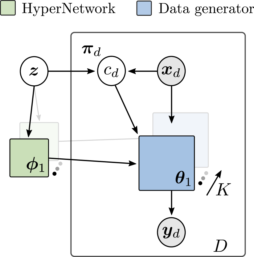
(a) Generative model

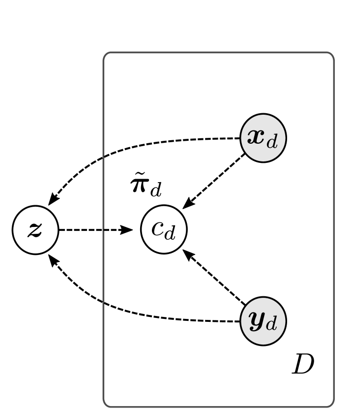
(b) Inference model

Figure 1: The VAMoH generative (a) and inference (b) model.

Notation.

We denote $[D]=\{1\dots D\}$ to the set of positive integers from 1 to D. Let $(\bm{X}^{(i)},\bm{Y}^{(i)})$, $i\in[N]$ be a set of $N$ data samples (e.g., images). The $i$-th sample comprises a point cloud of $D_{i}$ coordinate vectors, $\bm{X}^{(i)}\doteq\{\bm{x}^{(i)}_{j}\}_{j=1}^{D_{i}}$, and the set of corresponding feature vectors $\bm{Y}^{(i)}\doteq\{\bm{y}^{(i)}_{j}\}_{j=1}^{D_{i}}$. Let $\mathcal{X}$ and $\mathcal{Y}$ denote the space of coordinate and feature vectors, respectively. As an example, in the context of image analysis, $D_{i}$ represents the number of pixels in image $i$, and $(\bm{X}^{(i)},\bm{Y}^{(i)})$ correspond to the set of $\mathbb{R}^{2}$ coordinates and values (e.g. RGB values) of the pixels, respectively.

3.1 Mixture of HyperGenerators

VaMoH  generates a feature set $\bm{Y}$ given a set of corresponding coordinates $\bm{X}$. For simplicity, let us assume that $(\bm{X},\bm{Y})$ is an image with $D$ pixels. To generate such an image, first a continuous latent variable $\bm{z}$ is sampled from a prior distribution $p_{\bm{\psi}_{z}}(\bm{z})$ parameterized by $\bm{\psi}_{z}$. The resulting vector $\bm{z}$ acts as the input to $K$ different hypergenerators. Here, we refer as a hypergenerator to both an MLP-based hypernetwork $g_{\phi_{k}}(\bm{z})$, with input $\bm{z}$ that outputs a set of parameters $\bm{\theta}_{k}=g_{\phi_{k}}(\bm{z})$; and, a data generator, $f_{\theta_{k}}$, parametrized by the output of the hypernetwork. Thus, both $\bm{z}$ and $\bm{\theta}_{1},\ldots,\bm{\theta}_{K}$ encode the information shared among the $D$ coordinates (e.g., pixel location) in the data (e.g., pixel values) generation process.

In order for the resulting model to be expressive and interpretable, we assume that each pixel is sampled from a mixture of $K$ hypergenerators. Thus, for each pixel $d\in[D]$, we introduce a latent categorical variable $c_{d}\in[K]$ in order to select the hypergenerator responsible of the pixel distribution, such that

$$\begin{gathered}p_{\psi_{c}}(\bm{C}|\bm{X},\bm{z})=\prod_{d=1}^{D}\prod_{k=1}^{K}\pi_{dk}^{\llbracket c_{d}=k\rrbracket},\end{gathered}$$ (2)

where $\llbracket c_{d}=k\rrbracket$ is the indicator function. The probability mass function (pmf) of $c_{d}$ is also parameterized using a neural network $f_{\psi_{c}}$ with parameters $\psi_{c}$ that takes both $\bm{x}_{d}$ and $\bm{z}$ as input, and outputs $\bm{\pi}_{d}=f_{\psi_{c}}(\bm{x}_{d},\bm{z})$ using a soft-max function, where $\pi_{dk}=P(c_{d}=k|\bm{x}_{d},\bm{z})$.

In summary, the overall generative process is given by:

$$p(\bm{Y},\bm{C},\bm{z}|\bm{X})=p_{\psi_{z}}(\bm{z})\prod_{d=1}^{D}\prod_{k=1}^{K}\pi_{dk}^{\llbracket c_{d}=k\rrbracket}\,p_{\bm{\theta_{k}}}(\bm{y}_{d}|\bm{x}_{d}),$$ (3)

where, importantly, we rely on Random Fourier Features (RFF) (Tancik et al., 2020) to encode $\bm{x}_{d}$ to capture high frequency details with our generative functions $f_{\bm{\theta}}$, as in Dupont et al. (2022b).

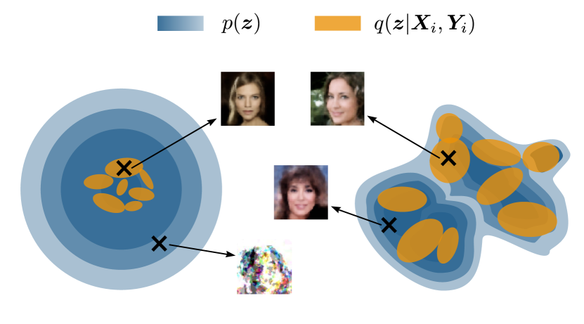
Figure 2: Illustration of the prior hole problem. Blue contours are the prior $p(\bm{z})$, whilst orange contours are approximate posteriors $q(\bm{z}|\bm{X}_{i},\bm{Y}_{i})$. Left: simple standard prior does not accurately cover the encoder complexity. Decoding samples from the prior that fall far from the aggregated posterior from training data gives unrealistic images. Right: a more flexible prior properly matches the complexity of the encoder, leading to better quality of the images generated from the prior.

Flow-based prior on $\bm{z}$.

The use of a fixed prior distribution for generating new unconditional samples in VAEs often results in the well-documented prior hole problem  (Rezende & Viola, 2018), illustrated in Figure 2. This limitation stems from the poor expressiveness of a fixed prior distribution as compared to the approximate posterior. To tackle this issue, we rely on normalizing flows (NF) to learn a prior distribution of the form $p_{\psi_{z}}(\bm{z})$ with parameters $\psi_{z}$. This improves the prior expressiveness and, thus, addresses the aforementioned problem. Specifically, VaMoH  integrates $T$ layers of a planar flow (Rezende & Mohamed, 2015) with a Gaussian $p_{0}(\bm{z})$ as base distribution, resulting in a flexible prior distribution that significantly enhances the generated samples. Extended empirical analysis is provided in Appendix A.5.

3.2 Inference model

In this subsection, we present the inference model that we propose to approximate the posterior of the latent variables $\bm{z}$ and $\bm{C}$. The model is defined as follows:

$$q_{\bm{\gamma}}(\bm{z},\bm{C}|\bm{Y},\bm{X})=q_{\bm{\gamma}_{z}}(\bm{z}|\bm{Y},\bm{X})\prod_{d=1}^{D}q_{\bm{\gamma}_{c}}(c_{d}|\bm{z},\bm{y}_{d},\bm{x}_{d}).$$ (4)

We illustrate the inference model in Figure 1(b). Throughout the following, we refer to all the parameters of the inference model as $\bm{\gamma}=\{\bm{\gamma}_{z},\bm{\gamma}_{c}\}$.

Inference for the continuous latent variable.

We propose to model the posterior distribution of $\bm{z}$ as $q_{\bm{\gamma}_{z}}(\bm{z}|\bm{Y},\bm{X})=\mathcal{N}\left(\bm{z}|f_{\bm{\gamma}_{z}}(\bm{Y},\bm{X})\right)$, parameterized by $\bm{\gamma}_{z}$. It’s important to note that this distribution is shared among the complete sample (e.g., image), thus $\bm{z}$ contains global information. To parametrize $f_{\bm{\gamma}_{z}}$, we use a PointConv (Wu et al., 2019). This entails several advantages. Firstly, it generalizes convolutional operations to continuous space coordinate systems, in contrast to the fixed grids used in CNNs (LeCun et al., 1995). Secondly, it is independent of data resolution, geometry of the grid, and missingness of the data. Of particular interest is the latter, as grid-based architectures typically require missing dimensions to be filled (e.g., with zeros), which introduces bias to the model (Simkus et al., 2021).

Inference of the mixture components.

We model the posterior over the categorical latent variables $c_{d}$ of each coordinate $d$ as

$$q_{\bm{\gamma}_{c}}(c_{d}|\cdot)=\text{Cat}\left(c_{d}|f_{\bm{\gamma}_{c}}(\bm{z},\bm{y}_{d},\bm{x}_{d})\right)=\prod_{k=1}^{K}\tilde{\pi}_{dk}^{\llbracket c_{d}=k\rrbracket},$$ (5)

where we parametrize $\bm{\gamma}_{c}$ with a simple MLP. It is important to notice that this posterior depends on the local information of the coordinate, i.e., $(\bm{x}_{d},\bm{y}_{d})$, and only on the global information through $\bm{z}$. This choice is made to encourage the model to learn to use different hypergenerators for different parts of the data.

3.3 Training

The evidence lower bound (ELBO) of our proposed model is given by

$$\mathcal{L}( \bm{X},\bm{Y})=\mathbb{E}_{q_{\gamma}}\left[\log p_{\bm{\theta}}\left(\bm{Y}|\bm{z},\bm{X},\bm{C}\right)\right]$$

$$-D_{KL}(q_{\gamma_{z}}(\bm{z}|\bm{X},\bm{Y})||p_{\psi_{z}}(\bm{z}))$$ (6)

$$-\mathbb{E}_{q_{\gamma_{z}}}\left[D_{KL}(q_{\gamma_{c}}(\bm{C}|\bm{z},\bm{X},\bm{Y})||p_{\psi_{c}}(\bm{C}|\bm{z},\bm{X}))\right].$$

We provide the complete derivation in Section A.2. We train VaMoH maximizing this ELBO by stochastic gradient descent on randomly selected mini-batches. To stabilize the initialization of the normalizing flow and accelerate convergence, we employ a standard prior $p(\bm{z})=\mathcal{N}(\bm{0},\bm{I})$ during the initial epochs of the training to allow the model to focus on organizing the approximate posterior and producing accurate reconstructions. After some iterations, we start training the Planar Flow $p_{\psi_{z}}(\bm{z})$. While KL between discrete distributions in Section 3.3 is easily computed in closed form, the continuous KL is approximated by Monte Carlo sampling, just as we do for the reconstruction term.

Table 1: Comparison of FID and Precision and Recall scores of image generation for VaMoH, GASP, and Functa. Low FID, high precision, and high recall indicate the best performance. The best results are highlighted in bold. Note that for Functa and CelebA HQ we just report their FID value, since they do not report the precision and recall.

	CelebA HQ			Shapes3D
Model	$\downarrow$ FID	$\uparrow$ Precision	$\uparrow$ Recall	$\downarrow$ FID	$\uparrow$ Precision	$\uparrow$ Recall
GASP (Dupont et al., 2022b)	14.01 $\pm$ 0.18	0.81 $\pm$ 0.0	0.43 $\pm$ 0.01	118.66 $\pm$ 0.64	0.01 $\pm$ 0.0	0.16 $\pm$ 0.01
Functa (Dupont et al., 2022a)	40.40	-	-	57.81 $\pm$ 0.15	0.06 $\pm$ 0.0	0.13 $\pm$ 0.0
VaMoH	66.27 $\pm$ 0.18	0.65 $\pm$ 0.0	0.0 $\pm$ 0.0	56.25 $\pm$ 0.57	0.08 $\pm$ 0.0	0.64 $\pm$ 0.01

Point dropout.

The design of VAMoH allows for easily handling point clouds $\{\bm{X},\bm{Y}\}$ of arbitrary sizes. The PointConv encoder is able to convolve the observed points, regardless of their coordinates, and map them into the approximate posterior, which can then be decoded to generate new points at any desired location. To enhance the conditional generation capabilities and robustness of VAMoH in inferring information from partial data, we apply dropout to the points within a set $\{\bm{X},\bm{Y}\}$ according to a probability $p\sim U(0,\alpha)$, which is sampled independently for each batch. The maximum dropout probability, $\alpha$, is fixed for ensuring that the reduced set contains at least as many points as centroids to be found at the first layer of PointConv. In previous VAE-based models (Ma et al., 2020; Peis et al., 2022), this strategy has been successfully employed for masking training batches in order to improve missing data imputation tasks. Nevertheless, since these models deal with grid-type incomplete data, some pre-imputation is required before feeding the encoder, mean imputation or zero filling being typical choices, with the cost of introducing bias in the model (Simkus et al., 2021). In contrast, in our work, the PointConv encoder easily handles missing data, without requiring any pre-imputation strategy. Additional empirical evaluations can be found in the Appendix A.4.

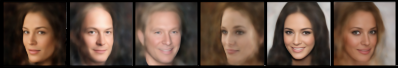
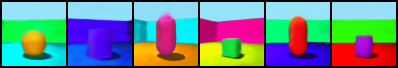
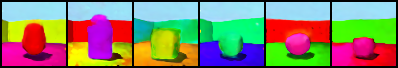
Functa    GASP    VaMoH    Functa    GASP    VaMoH   

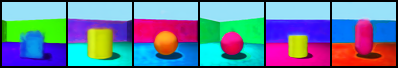
Figure 3: Comparison of generation quality at original resolution. CelebA HQ samples of Functa obtained from (Dupont et al., 2022a).

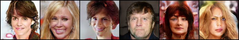
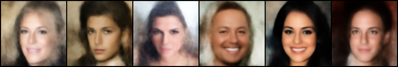
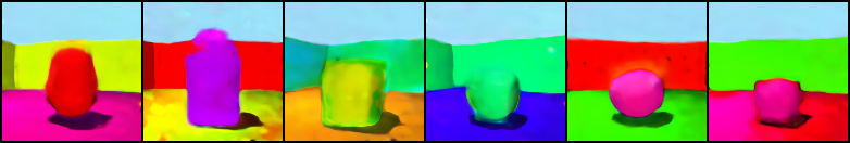
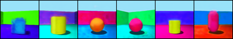
GASP    VaMoH    GASP    VaMoH    GASP       VaMoH   

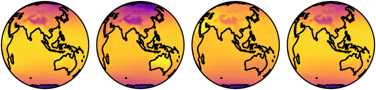
Figure 4: Comparison of uncurated generated samples at super-resolution.

4 Experiments

In this section, we provide a thorough empirical evaluation of VaMoH. We evaluate our model on the tasks of data generation, reconstruction, and imputation, including the superresolution results.

Baselines.

We compare VaMoH with GASP (Dupont et al., 2022b) and Functa (Dupont et al., 2022a) with a Normalizing Flow as generator of modulation vectors, which we denote simply by Functa. More specifically, GASP is only considered for data generation, since it does not allow for any inference-related task.

Datasets.

We evaluate VaMoH on PolyMNIST ($28\times$28), CelebA HQ ($64\times$64) (Karras et al., 2017), Shapes3D ($64\times$64) (Burgess & Kim, 2018), climate data from the ERA5 dataset (Hersbach et al., 2019), and 3D chair voxels from the ShapeNet dataset (Chang et al., 2015). The architecture and hyperparameters used for each dataset are detailed in Section B.1.

We implemented VaMoH in PyTorch and performed all experiments on a single V100 with 32GB of RAM. The code with the model implementation and experiments is available at https://github.com/bkoyuncu/vamoh. In this section, we provide a glimpse into the results of our experiments on all datasets. Additional experiments and their outcomes can be found at Appendix B.

4.1 Generation

In this section, we evaluate VaMoH for the task of synthetic data generation over continuous coordinate systems. Samples are obtained from the learned models in both the original and twice the resolution, referred to as super resolution.

Metrics.

We use two metrics to evaluate the quality of the generated samples. We report the usually employed Fréchet Inception Distance (FID) (Heusel et al., 2017) as well as the improved precision and recall (Kynkäänniemi et al., 2019), which measures the quality of the generated data (i.e, high precision) and the coverage of the true data distribtuion (i..e, high recall).

Results.

We present the summary of the quantitative comparison of VaMoH with both baselines for two image datasets in Table 1. Our analysis indicates that, quantitatively speaking, there is not a clear winner among the models. While GASP achieves the highest performance on the CelebA HQ dataset, visual inspection of the generated samples in Figure 3 reveals that the quality of Functa  and VaMoH is also high. This aligns with previous studies (Dupont et al., 2022a) that have noted that FID may over-penalize blurriness. Additionally, it is worth noting that VaMoH obtains a recall of 0.0 on this dataset, despite the generated samples displaying diversity in features such as facial expressions and hairstyles, as seen in Figure 3. In analyzing the performance of VaMoH on the Shapes3D dataset, we observe a clear superiority compared to other models. As depicted in Figure 3, VaMoH is able to generate objects with diverse shapes and colors, as well as walls and floors delimited with sharp edges. Furthermore, it achieves the highest quantitative metrics, as demonstrated in the right columns of Table 1. Despite this, it is important to note that the low precision values obtained by all models require a comprehensive evaluation approach, incorporating both quantitative and qualitative metrics when assessing generative models.

Finally, in Figure 4, we evaluate the super-resolution capabilities of the models by visually inspecting the generated samples at twice the original resolution. We utilize the same latent code as in the generated samples in Figure 3 for the CelebA HQ and Shapes3D datasets. Additionally, to demonstrate the versatility of our VaMoH to model diverse types of data, we also include super resolution samples from the ERA5 dataset. Comparison with super-resolution samples generated by Functa, and additional results for all the datasets can be found in Section B.2.

Discussion.

A significant advantage of VaMoH is its ability to achieve the capability of generation through a single optimization procedure. In contrast, GASP requires solving the min-max GAN optimization, which has been acknowledged to be unstable (Jabbar et al., 2020); and Functa requires first learning the SIREN model and modulations for each sample, followed by the training of an additional generative model, such as a normalizing flow.

Overall, these results demonstrate that the generation quality of VaMoH is comparable to existing alternatives. In the following, we show that VaMoH exhibits superior efficiency and performance in inference tasks in comparison with Functa. It is worth noting that we do not compare VaMoH with GASP, as it is purely a generative model.

Ground truth

Reconstructions
Super-reconstructions

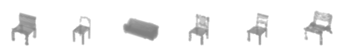
Functa    VaMoH   

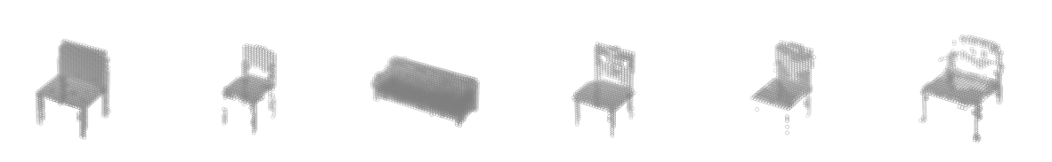
Functa    VaMoH   

(a) ShapeNet

Ground truth

Reconstructions Super-reconstructions

Functa    VaMoH   

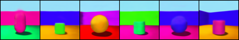
Functa    VaMoH   

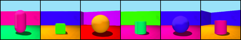
(b) Shapes3D

Figure 6: Comparison of reconstruction quality of VaMoH and Functa on ground truth data from the first samples of the test set at original and super-resolution.

4.2 Reconstruction

Table 2: Comparison of inference time (seconds) for reconstruction task of VaMoH and Functa. On the right-most two columns, we show the speed improvement of VaMoH compared to Functa (3) which is trained with 3 gradient steps as suggested in the original paper (Dupont et al., 2022a) and Functa (10) which is trained with 10 gradient steps to obtain the results of Functa depicted in Figures 21,23. Please note that these experiments are run on the same GPU device.

	Model Inference Time (secs)			Speed Improvement
Dataset	VaMoH	Functa (3)	Functa (10)	vs. Functa (3)	vs. Functa (10)
PolyMNIST	0.00453	0.01648	0.05108	x 3.64	x 11.28
Shapes3D	0.00536	0.01759	0.05480	x 3.28	x 10.22
CelebA HQ	0.00757	0.01733	0.05381	x 2.29	x 7.11
ERA5	0.00745	0.01899	0.05932	x 2.55	x 7.96
ShapeNet	0.00689	0.02095	0.06576	x 3.04	x 9.54

In this section, we evaluate the performance of VaMoH in reconstructing data and compare it with Functa. As before, we conduct the assessment at both the original resolution and at double the resolution, which we refer to as super-reconstruction. This latter scenario involves generating features at new coordinate positions.

Metrics.

We use the Peak Signal-to-Noise-Ratio (PSNR) to quantify the quality of reconstructions (See Section B.3 for further details). We also compare inference times (in seconds) of VaMoH and Functa in Tables 2 and 5.

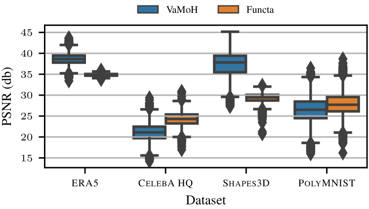
Figure 7: Comparison of PSNR (db) of reconstructed images in the test set.

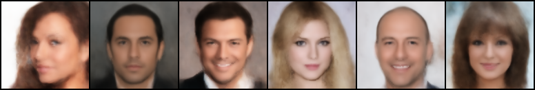
Ground truth Super-reconstruction Ground truth Super-reconstruction

Figure 8: Ground truth for the first six test set samples and the corresponding super-reconstruction obtained by VaMoH for CelebA HQ and ERA5 datasets.

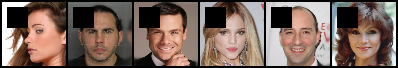
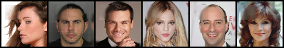
In    Recons.    In    Recons.   

(a) Missing a patch

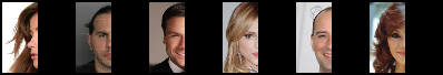
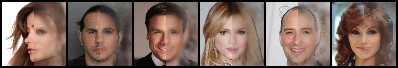
In    Recons.    In    Recons.   

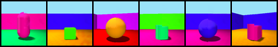
(b) Missing half of the image

Figure 9: Imputation of different amounts of missing parts using VaMoH. For each dataset, the top row shows the input with the missing part (In) and the bottom row shows the reconstructed image.

Results.

Figure 6 shows reconstructions and super-reconstructions for the first 6 samples of the test set of ShapeNet and Shapes3D for Functa and VaMoH. We observe that both methods produce high-quality reconstructions. When evaluating the ShapeNet dataset (as shown in Figure 6(a)), we observe that both models are capable of capturing the details of the chairs, such as the various patterns present on the back of the chairs. Notably, VaMoH achieves more detailed edges in both reconstructions and super-reconstructions for the Shapes3D dataset (see Figure 6(b)) as well as overall less blurriness. A more quantitative assessment is provided in Figure 7, which compares PSNR values obtained for all the test set samples of the image-like datasets. We observe that VaMoH achieves similar quality on PolyMNIST and CelebA HQ, and outperforms Functa on ERA5 and Shapes3D. This is quite remarkable as Functa requires solving an optimization problem per sample, and thus it ‘overfits’ each of the samples. In stark contrast, VaMoH efficiently generates reconstructions with a single forward pass. As a consequence, VaMoH is significantly faster. In Table 2, we show that VaMoH is more than 2 times faster than Functa when trained with 3 gradient steps (as stated in (Dupont et al., 2022a)); and at least 7 times faster when trained with 10 gradient steps. Finally, Figure 8 shows the ability of VaMoH to generate quality super-reconstructions on the CelebA HQ and ERA5 datasets. Another inference time comparison for super-reconstruction can be found in Table 5 in Appendix B.3.

Discussion.

Both VaMoH and Functa are able to reconstruct and super-reconstruct data with high quality with different data modalities (e.g., images and voxels). On top of this, VaMoH achieves comparable or better PSNR values for the test set, which indicates it may reconstruct more details. Additionally, in Table 2, we show that VaMoH is significantly faster than Functa for the reconstruction task. This happens because VaMoH requires a simple forward pass. In contrast, Functa requires finding a new modulation for each new sample, which is an optimization in itself; therefore, its inference time highly depends on the number of gradient steps needed, which does not only have a major impact on the quality of the results but also on its computational efficiency. Note that this computational burden applies to any inference-related task, e.g., image completion. Given the quantitative and qualitative assessment of the results of VaMoH, we argue that it might be preferable to rely on VaMoH due to its inference time efficiency in comparison to Functa. Thus, in the following, we keep understanding the capabilities of VaMoH without comparison.

4.3 Image completion

We evaluate the performance of VaMoH on the task of image completion. We consider two scenarios: (i) missing a patch (i.e., image in-painting) and (ii) missing half of the image, as a challenging case. Figure 9 illustrates the results on unseen test samples from CelebA HQ and Shapes3D. Our results demonstrate that VaMoH can reconstruct high-quality images, even when half of the image is missing, as in Figure 9(b). Thanks to the use of PointConv (Wu et al., 2019) as the encoder, VaMoH can infer missing information without the need of inputting dummy values (e.g., zeros) for the features of the missing coordinates. This is something needed in standard VAEs, and allows VaMoH to mitigate any potential biases in the results. Complete results for all datasets evaluated, including those for image out-painting, can be found in Section B.4.

4.4 The flexibility of VAMoH

In this Section, we provide evidence of the interpretability of VaMoH. In particular, we show an example in which the mixture of hypergenerators, with $K=4$, allows for splitting the generation of each pixel into several modes.

In Figure 10, we show the entropy (middle row) and map (bottom row) of the posterior distribution of the categorical latent variables $\bm{C}$. By examining the entropies per pixel, we observe low values for most pixels, but higher values for the borders. This indicates that the model is uncertain about which components to use at the borders, while it is using fewer components for the rest of the image. Furthermore, the map values of $\bm{C}$ resemble a segmentation map. Here, we observe that one hypergenerator (orange) is specialized in filling the colors of different parts of the image, while the others (blue, red, and green) are used for the borders.

Recons.    $\bm{C}_{\text{ent}}$    $\bm{C}_{\text{map}}$   

Figure 10: Reconstructed samples (top), entropy (middle) $\bm{C}_{\text{ent}}=\mathcal{H}(\bm{C}|\bm{Y},\bm{X})$, and map (bottom) $\bm{C}_{\text{map}}=\max_{c_{d}}q_{\bm{\gamma}_{c}}(\bm{C}|\bm{Y},\bm{X})$ of the posterior distribution over the mixture.

5 Conclusion

In this paper, we introduced VaMoH, a novel VAE-based model for learning distributions of functions that enables efficient and accurate generation of data over continuous coordinate systems. Notably, VaMoH allows for straightforward conditional generation with a simple forward pass on the model. VaMoH can perform tasks such as in-painting and out-painting or generate higher-resolution versions of a test set sample (that is, unseen during training) more efficiently than competing methods. Our experimental results demonstrate the effectiveness of VaMoH, both in generation and inference tasks, in a wide range of applications and datasets.

Although our model has a couple of limitations, they are not significant factors that would impede its effectiveness. Firstly, one limitation relates to the number of parameters in the hypernet, which scales linearly with the number of components (i.e., $K$). Secondly, we could improve the speed of the PointConv encoder with a sampling-based algorithm for the selection of centroid points used for the convolution step.

As a future research direction, we aim to enhance VaMoH by exploring methods for achieving disentanglement in the latent space. This would allow for controlled modifications of generated and reconstructed samples and may open up new possibilities for applications such as data editing at various resolutions. We have not identified any social concerns associated with this work. In fact, VaMoH reduces the time required for inference during testing, which could broaden the range of applications and areas where INR methods can be utilized.

6 Acknowledgements

Batuhan Koyuncu and Isabel Valera acknowledge the support by the German Federal Ministry of Education and Research (BMBF) through the Cell-o project. Pablo Sánchez Martín thanks the German Research Foundation through the Cluster of Excellence “Machine Learning – New Perspectives for Science”, EXC 2064/1, project number 390727645 for generous funding support. The authors thank the International Max Planck Research School for Intelligent Systems (IMPRS-IS) for supporting Pablo Sánchez Martín. Pablo M. Olmos and Ignacio Peis acknowledge the support by the Spanish government MCIN/AEI/10.13039/501100011033/ FEDER, UE, under grant PID2021-123182OB-I00, by Comunidad de Madrid under grant IND2022/TIC-23550, and by Comunidad de Madrid and FEDER through IntCARE-CM. The work of Ignacio Peis has been also supported by the Spanish government (MIU) under grant FPU18/00516. We thank Adrián Javaloy and Jonas Klesen for their valuable comments and discussions.

Appendix A Further details about VaMoH

A.1 HyperGenerator networks

As a reminder, we work with data samples which are point clouds $(\bm{X},\bm{Y})$ with coordinate vectors $\bm{X}$ and feature vectors $\bm{Y}$. VaMoH aims to generate a feature set $\bm{Y}$ given a set of corresponding coordinates $\bm{X}$. If the data sample is an image with $D$ pixels, $(\bm{X},\bm{Y}$) correspond to the set of $\mathbb{R}^{2}$ coordinates and values (e.g. RGB values) of the pixels, respectively.

To generate such an image, first a continuous latent variable $\bm{z}$ is sampled from a prior distribution $p_{\bm{\psi}_{z}}(\bm{z})$ parameterized by $\bm{\psi}_{z}$. The resulting vector $\bm{z}$ can be thought as a global summary vector of the output image and acts as the input to $K$ different hypergenerators. Here, we refer as a hypergenerator to both an MLP-based hypernetwork $g_{\phi_{k}}(\bm{z})$, with input $\bm{z}$ that outputs a set of parameters $\bm{\theta}_{k}=g_{\phi_{k}}(\bm{z})$; and, a data generator, $f_{\theta_{k}}$, parametrized by the output of the hypernetwork as shown in Figure 1. In other words, each of the MLP-based hypernetwork outputs the set of parameters $\bm{\theta}_{k}=g_{\phi_{k}}(\bm{z})$ that parameterizes the corresponding data generator $f_{\theta_{k}}$ which operates over each input coordinate $\bm{x}_{d}\in\bm{X}$ to generate corresponding feature values $\bm{y}_{d}\in\bm{Y}$, i.e. $\bm{y}_{d}=f_{\theta_{k}}(\bm{x}_{d})$ where $d\in[D]$.

The intuition for the usage of hypergenerators can be explained as follows: VaMoH uses a continous latent variable $\bm{z}$ as an input to a hypernetwork. This hypernetwork is used for parameterizing a data generator, i.e. an INR, that can model a data sample. In the inference step, VaMoH can infer the latent variable $\bm{z}$ using a PointConv based encoder. Therefore, VaMoH can perform conditional tasks by performing an inference step. Moreover, each of the conditional tasks requires only a single forward pass without any extra optimization step per samples. Lastly, $K$ different hypergenerators increase the expresiveness of VaMoH since they act as separate INRs for modeling different patterns in the output.

A.2 ELBO derivation

Our objective is to maximize the evidence lower bound (ELBO) of a set of $D$ features $\bm{Y}$ given the corresponding set of coordinates $\bm{X}$. To do so, we introduce a family of variational distributions for the continuous and discrete latent variables, namely $\bm{z}$ and $c_{d}$ where $d\in[D]$:

$$q_{\bm{\gamma}}(\bm{z},\bm{C}|\bm{Y},\bm{X})=q_{\bm{\gamma}_{z}}(\bm{z}|\bm{Y},\bm{X})\prod_{d=1}^{D}q_{\bm{\gamma}_{c}}(c_{d}|\bm{z},\bm{y}_{d},\bm{x}_{d}).$$ (7)

where

$$q_{\bm{\gamma}_{z}}(\bm{z}|\bm{Y},\bm{X})=\mathcal{N}\left(\bm{z}|f_{\bm{\gamma}_{z}}(\bm{Y},\bm{X})\right)\quad\text{ and }\quad q_{\bm{\gamma}_{c}}(c_{d}|\bm{z},\bm{y}_{d},\bm{x}_{d})=\text{Cat}\left(c_{d}|f_{\bm{\gamma}_{c}}(\bm{z},\bm{y}_{d},\bm{x}_{d})\right).$$ (8)

Note that these two distributions are parameterized by $\bm{\gamma}_{z}$ and $\bm{\gamma}_{c}$, which we aim to learn. We refer to the set of all inference parameters as $\bm{\gamma}=\{\bm{\gamma}_{z},\bm{\gamma}_{c}\}$. Moving on to the generative distribution, it factorizes as

$$p_{\psi,\phi}(\bm{Y},\bm{C},\bm{z}|\bm{X})=p_{\bm{\theta}}(\bm{Y}|\bm{X},\bm{C},\bm{z})p_{\psi_{c}}(\bm{C}|\bm{z},\bm{X})p_{\psi_{z}}(\bm{z})$$ (9)

where $p_{\psi_{c}}(\bm{C}|\bm{z},\bm{X})$ is the prior over the categorical latent variable, $p_{\psi_{z}}(\bm{z})$ is the prior over the continuous latent variable (parameterized by a Normalizing Flow, see Section A.5), and $p_{\bm{\theta}}(\bm{Y}|\bm{X},\bm{C},\bm{z})$ is the likelihood distribution over the set of features. More in detail, the likelihood factorizes over coordinates and we define each of them as a mixture:

$$p_{\bm{\theta}}(\bm{Y}|\bm{X},\bm{C},\bm{z})=\prod_{d=1}^{D}p_{\bm{\theta}}(\bm{y}_{d}|\bm{x}_{d},c_{d},\bm{z}),=\prod_{d=1}^{D}\prod_{k=1}^{K}\pi_{dk}^{\llbracket c_{d}=k\rrbracket}\,p_{\bm{\theta}_{k}}(\bm{y}_{d}|\bm{x}_{d})\quad\text{ where }\quad\bm{\theta}_{k}=g_{\phi_{k}}(\bm{z}).$$ (10)

At this point, it is important to remark that we do not learn the parameters $\bm{\theta}_{k}$ $k\in[K]$ of the likelihood directly. Instead, we learn $k$ the parameters of $k$ different hypernetworks $g_{\phi_{k}}$ $k\in[K]$ that output the corresponding likelihood parameters. Thus, the set of all the parameters of the generative models are $\bm{\phi}=\{\bm{\phi}_{k}\}_{k=1}^{K}$ and $\bm{\psi}=\{\psi_{z},\psi_{c}\}$.

With this choice of the inference and generative model, we define the ELBO as

$$\mathcal{L}(\bm{Y},\bm{X};\psi,\phi,\bm{\gamma})=\mathbb{E}_{q_{\bm{\gamma}}(\bm{z},\bm{C}|\bm{Y},\bm{X})}\left[\log\frac{p_{\psi,\phi}(\bm{Y},\bm{C},\bm{z}|\bm{X})}{q_{\bm{\gamma}}(\bm{z},\bm{C}|\bm{Y},\bm{X})}\right]\leq\log p(\bm{Y}|\bm{X}).$$ (11)

Using the factorization of the generative and inference model in Equations 8 and 10, we can split it in various terms:

$$\mathcal{L}(\bm{Y},\bm{X};\psi,\phi,\bm{\gamma}) =\mathbb{E}_{q_{\bm{\gamma}}(\bm{z},\bm{C}|\bm{Y},\bm{X})}\left[\log p_{\bm{\theta}}(\bm{Y}|\bm{X},\bm{C},\bm{z})\right]$$

$$+\mathbb{E}_{q_{\bm{\gamma}}(\bm{z},\bm{C}|\bm{Y},\bm{X})}\left[\log\frac{p_{\psi_{z}}(\bm{z})}{q_{\bm{\gamma}_{z}}(\bm{z}|\bm{Y},\bm{X})}\right]$$

$$+\mathbb{E}_{q_{\bm{\gamma}}(\bm{z},\bm{C}|\bm{Y},\bm{X})}\left[\log\frac{p_{\psi_{c}}(\bm{C}|\bm{z},\bm{X})}{q_{\bm{\gamma}_{c}}(\bm{C}|\bm{z},\bm{Y},\bm{X})}\right]$$ (12)

We can marginalize some variables from the expectations.

$$\mathcal{L}(\bm{Y},\bm{X};\psi,\phi,\bm{\gamma}) =\mathbb{E}_{q_{\bm{\gamma}}(\bm{z},\bm{C}|\bm{Y},\bm{X})}\left[\log p_{\bm{\theta}}(\bm{Y}|\bm{X},\bm{C},\bm{z})\right]$$

$$+\mathbb{E}_{q_{\bm{\gamma}_{z}}(\bm{z}|\bm{Y},\bm{X})}\left[\log\frac{p_{\psi_{z}}(\bm{z})}{q_{\bm{\gamma}_{z}}(\bm{z}|\bm{Y},\bm{X})}\right]$$

$$+\mathbb{E}_{q_{\bm{\gamma}}(\bm{z},\bm{C}|\bm{Y},\bm{X})}\left[\log\frac{p_{\psi_{c}}(\bm{C}|\bm{z},\bm{X})}{q_{\bm{\gamma}_{c}}(\bm{C}|\bm{z},\bm{Y},\bm{X})}\right]$$ (13)

And rewriting the last two terms as KL divergences we get:

$$\mathcal{L}(\bm{Y},\bm{X};\psi,\phi,\bm{\gamma}) =\mathbb{E}_{q_{\bm{\gamma}}(\bm{z},\bm{C}|\bm{Y},\bm{X})}\left[\log p_{\bm{\theta}}(\bm{Y}|\bm{X},\bm{C},\bm{z})\right]$$

$$-D_{KL}(q_{\gamma_{z}}(\bm{z}|\bm{X},\bm{Y})||p_{\psi_{z}}(\bm{z}))$$

$$-\mathbb{E}_{q_{\bm{\gamma}}(\bm{z}|\bm{Y},\bm{X})}\left[D_{KL}(q_{\gamma_{c}}(\bm{C}|\bm{z},\bm{X},\bm{Y})||p_{\psi_{c}}(\bm{C}|\bm{z},\bm{X}))\right].$$ (14)

Finally, in the first term, we can marginalize over the categorical latent variable such that we only need to approximate by Monte Carlo expectation over $\bm{z}$:

$$\mathbb{E}_{q_{\bm{\gamma}}(\bm{z},\bm{C}|\bm{Y},\bm{X})}\left[\log p_{\bm{\theta}}(\bm{Y}|\bm{X},\bm{C},\bm{z})\right] =\mathbb{E}_{q_{\bm{\gamma}}(\bm{z},\bm{C}|\bm{Y},\bm{X})}\left[\sum_{d=1}^{D}\log p_{\bm{\theta}}(\bm{y}_{d}|\bm{x}_{d},\bm{z},c_{d})\right]$$

$$=\sum_{d=1}^{D}\mathbb{E}_{q_{\bm{\gamma}_{z}}(\bm{z}|\bm{Y},\bm{X})}\left[\sum_{k=1}^{K}\log p_{\bm{\theta}_{k}}(\bm{y}_{d}|\bm{x}_{d})\cdot\pi_{dk}\right]$$ (15)

Then ELBO becomes

$$\mathcal{L}(\bm{Y},\bm{X};\psi,\phi,\bm{\gamma}) =\sum_{d=1}^{D}\mathbb{E}_{q_{\bm{\gamma}_{z}}(\bm{z}|\bm{Y},\bm{X})}\left[\sum_{k=1}^{K}\log p_{\bm{\theta}_{k}}(\bm{y}_{d}|\bm{x}_{d})\cdot\pi_{dk}\right]$$

$$-D_{KL}(q_{\gamma_{z}}(\bm{z}|\bm{X},\bm{Y})||p_{\psi_{z}}(\bm{z}))$$

$$-\mathbb{E}_{q_{\bm{\gamma}}(\bm{z}|\bm{Y},\bm{X})}\left[D_{KL}(q_{\gamma_{c}}(\bm{C}|\bm{z},\bm{X},\bm{Y})||p_{\psi_{c}}(\bm{C}|\bm{z},\bm{X}))\right].$$ (16)

A.3 Algorithm details

The training methodology is outlined in Algorithm 1. As discussed in Section 3.3, the training process begins with an initial warming stage, in which a standard prior $p(\bm{z})$ is utilized to stabilize the optimization of the encoder. The second and primary stage involves the introduction of the learnable prior $p_{\psi_{z}}(\bm{z})$.

Algorithm 1 Minibatch training of VaMoH

1:  Define hyperparameters, estimator $\widetilde{\mathcal{L}}$ using Eq. (3.3)

2:  $\gamma_{z,c}$ (inference), $\psi_{z,c}$ (prior), $\phi_{1:K}$ (hypernetwork) $\leftarrow$ initialize

3:  repeat

4:     $\{\bm{X},\bm{Y}\}_{1:M}\leftarrow$ random minibatch of $M$

5:     $\{\bm{X^{\prime}},\bm{Y^{\prime}}\}_{1:M}\leftarrow$ apply dropout with probability $p\sim U(0,\alpha)$

6:     if NF is available then

7:        parameterize $p_{\psi}(\bm{z})$ with planar flow

8:     else

9:        fix $p(\bm{z})$ with standard Gaussian

10:     end if

11:     $\mathbf{g}\leftarrow\nabla_{\gamma,\psi,\phi_{1:K}}\widetilde{\mathcal{L}}^{M}\left(\gamma,\psi,\phi_{1:K};\{\bm{X},\bm{Y}\}_{1:M}\right)$ (gradients)

12:     $\gamma,\psi,\phi_{1:K}\leftarrow$ Update parameters using gradients $\mathbf{g}$

13:  until convergence of parameters $\gamma,\psi,\phi_{1:K}$

A.4 Point dropout for conditional generation

In this section, we present experimental evidence supporting the effectiveness of the point dropout strategy for training VAMoH, as discussed in Section 3.3 of the paper. Figure 11 illustrates the results of patch imputation on test images from the test set of CelebA HQ. When the model is trained on full images, as shown in Figure 11(a), the PointConv encoder is unable to learn from a diverse set of centroids, resulting in uninformative posteriors when partial images are used during testing. However, as shown in Figure 11(b), when VAMoH is trained on images that have undergone point dropout, as outlined in Section 3.3, improved robustness for conditional generation is obtained.

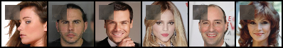
(a) Without point dropout

(b) With point dropout

Figure 11: Imputation of missing patches in test CelebA HQ images using VAMoH. In (a), full images are fed to the model during training. In (b), points of training images are deleted with a dropout probability per batch.

A.5 Flow-based prior

In this section, we evaluate the effectiveness of the Planar Flow as a prior for our continuous latent variable in addressing the hole problem described in Section 3.1. We first train our model on the CelebA dataset (Liu et al., 2015), utilizing a fixed standard prior $p(\bm{z})$. Upon convergence, we sample from the learned prior and present the results in Figure 12(a). The standard prior places significant probability mass in regions distant from the aggregated posterior, resulting in poor image quality when samples are drawn from these regions. By reducing the variance and approaching the posterior probability mass, as demonstrated in Figure 12(b), we observe improved realism in the generated images. However, this also leads to a lack of diversity in the generated samples. In Figure 12(c) we include decoded samples from the posterior parameterized by the flexible encoder that reveals diversity for reconstructing images.

In contrast, by introducing the Planar Flow after a warming stage and training its parameters, we observe a more aligned reconstruction-generation process. This is evident by comparing the samples obtained by sampling from the posterior (Figure 12(d)) and the learned prior (Figure 12(e)), respectively.

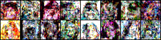
(a) Standard prior, $\bm{z}\sim\mathcal{N}(\bm{0},\bm{I})$

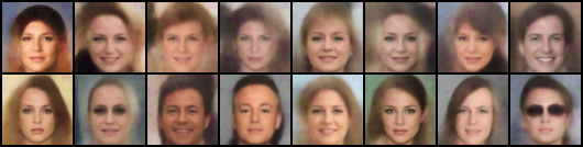
(b) Standard prior, $\bm{z}\sim\mathcal{N}(\bm{0},0.01\cdot\bm{I})$

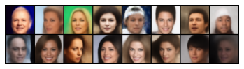
(c) Standard prior, $\bm{z}\sim q(\bm{z}|\bm{X},\bm{Y})$

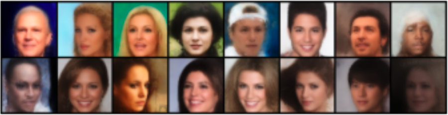
(d) Flow-based prior, $\bm{z}\sim q(\bm{z}|\bm{X},\bm{Y})$

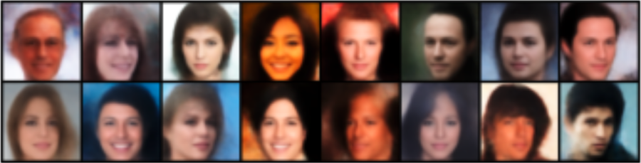
(e) Flow-based prior, $\bm{z}\sim p_{\psi_{z}}(\bm{z})$

Figure 12: Decoding samples from different latent distributions. Images in (a), (b), and (c) are generated/reconstructed by our model after being trained assuming a standard prior over $\bm{z}$. In (d) and (e) we include reconstructions and generations, respectively, when modeling a more flexible prior over $\bm{z}$ by training a Planar Flow.

A.6 Logistic likelihood

Inspired by (Kingma et al., 2016), we utilize a Discretized Logistic distribution for parameterizing the likelihood of discrete data with high number of categories, such as color channels in the RGB space for images. By doing that, we obtain a smooth and memory efficient predictive distribution for $\bm{y}_{d}$, as opposed to, for example, a Categorical likelihood with parameterized with 256-way softmax. The likelihood parameterized by each hypergenerator is given by

$$p_{\bm{\theta}_{k}}(\bm{y}_{d}|\bm{x}_{d})=\sigma\left(\left(\bm{y}_{d}+0.5-\bm{\mu}_{dk}\right)/\bm{s}\right)-\sigma\left(\left(\bm{y}_{d}-0.5-\bm{\mu}_{dk}\right)/\bm{s}\right),$$ (17)

where the means $\bm{\mu}_{dk}$ are outputs of the hypergenerator, and the scales $\bm{s}$ are learnable parameters. Thanks to the design of VAMoH, our approach using a mixture for the likelihood is in line with (Salimans et al., 2017), and results in a Discretized Logistic Mixture Likelihood of the form

$$p(\bm{y}_{d}|\bm{x}_{d})=\prod_{k=1}^{K}\pi_{k}\left[\sigma\left(\left(\bm{y}_{d}+0.5-\bm{\mu}_{dk}\right)/\bm{s}\right)-\sigma\left(\left(\bm{y}_{d}-0.5-\bm{\mu}_{dk}\right)/\bm{s}\right)\right],$$ (18)

which allows to accurately model the conditional distributions of the points by using a relatively small number of mixture components, as we show in our paper, and in concordance with (Salimans et al., 2017).

A.7 Effect of mixture components

Using a mixture of decoders which are parameterized by hypernetworks increases the expressiveness of our model as provide a mixture of INRs to map coordinates to features in the decoding step. Furthermore, it provides the flexibility of acquiring segmentation and entropy maps as shown in Figure 10. In addition, in Figure 13, we show the effect of not using a mixture (K=1), we have lower quality outputs. Moreover, if we increase too much the number of components (K=10), we achieve similar quality; however, we get over-segmented images where regions of interest are less informative.

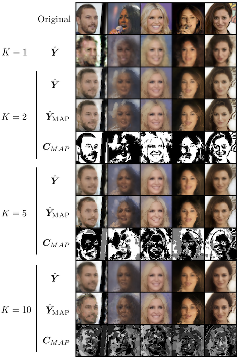
Figure 13: Ablation study on mixture of generators and effects of different number of mixture components in VaMoH for reconstruction task with CelebA HQ dataset.

Appendix B Experimental extension

In this section, we describe the experimental setup for VaMoH, as detailed in Appendix B.1. We also present a comprehensive set of results, including comparisons with the baselines Functa and GASP. Of note, we used the original code from GASP to replicate their results and also trained it on new datasets in our experimental setup. For Functa, we report results from the original paper (Dupont et al., 2022a) for the datasets shared with our study, and for the remaining datasets, we implemented and generated results independently with our own implementation.

B.1 Experimental setup

Implementation details for VaMoH are provided in Table 3. We base our choice of architecture on (Dupont et al., 2022b) as it provides a baseline setting. We train all of our model configurations with Adam optimizer. Also, in all of our models, we train Planar Flow and MLPs with activation of LeakyReLU with the exception of Sigmoid activation in the final layer of function generator. For datasets CelebA HQ, Shapes3D and PolyMNIST, Discretized Logistic likelihood (Kingma et al., 2016; Salimans et al., 2017) is utilized, whilst for ShapeNet and ERA5, Bernoulli and Continuous Bernoulli (Loaiza-Ganem & Cunningham, 2019) are employed, respectively.

Table 3: Implementation details of VaMoH.

		CelebA-HQ	Shapes3D	PolyMNIST	ShapeNet	Era5
	dim_z	64	32	16	32	32
	K	10	5	4	3	3
	epochs	1000	600	600	500	600
	bs	64	64	256	22	64
	lr	1e-4	1e-4	1e-3	1e-3	1e-4
PointConv Encoder	h_weights	[16,16,16,16]	[16,16]	[16,16]	[16,16,16,16]	[16,16,16,16]
	neighbors	[9,9,9,9,9]	[16,16,16]	[9,9,9]	[8,27,27,27,8]	[9,9,9,9,9]
	centroids	[4096,1024,256,64,1]	[1024,256,64]	[196,49,25]	[4096,512,64,16,16]	[1024,256,64,32,16]
	out_channels	[64,128,256,512,512]	[32,64,256]	[32,32,32]	[32,64,128,256,16]	[32,64,256,512,32]
	avg_pooling_neighbors	[9,9,9,9,None]	None	None	None	None
	avg_pooling_centroids	[1024,256,64,16,None]	None	None	None	None
Categorical Encoder	layers	[64,32]	[32,32]	[32,32]	[32,32]	[32,32]
Hypernetwork	layers	[256,512]	[128,256]	[16,32]	[256,512]	[256,512]
Generator	layers	[64,64,64]	[32,32]	[4,4,4]	[64,64,64]	[64,64,64]
	RFF	$\text{m}=128,\sigma=2$	$\text{m}=128,\sigma=2$	$\text{m}=128,\sigma=2$	$\text{m}=128,\sigma=2$	$\text{m}=128,\sigma=2$
Flow	T	80	20	3	40	10

B.2 Generation

In this section, we present a comprehensive evaluation of the generation capabilities of VaMoH in comparison to Functa and GASP. Table 4 contains the obtained values for the FID, Precision, and Recall metrics for the image datasets. These values are presented as the mean and standard deviation computed over five independent sets of generated images. For each of the metrics, we report the values using real embeddings coming from the training set (tr) and the test set (tst), since we also want to evaluate whether any model is overfitting to the training set, or as wished, it is able to generalize.

Results for the CelebA HQ and Shapes3D datasets were previously discussed in Section 4.1. Additionally, we include in this Section results for the PolyMNIST dataset, where we observe that GASP obtains the best quantitative results, which might be related to its ability to generate sharp samples. Quantitative values for Functa and PolyMNIST are not reported as they were not used in the original paper and we found that normalizing flows failed to avoid overfitting to the modulations, even when trying different values of dropout, number of layers, and dimensionality of the hidden space. This led to low quality of the generations, as shown in 17(b).

Visual inspection of the generated samples in Figure 15, Figure 17 illustrates that VaMoH generates high-quality samples, capturing details such as smiles in CelebA HQ  (Figure 15(a)), variety in chair legs in ShapeNet (Figure 15(b)), backgrounds in PolyMNIST (Figure 17(b)), as well as different configurations of temperatures (Figure 19). In Figure 15, Figure 17, we did not include generation samples of CelebA HQ and ShapeNet for Functa since we were unable to reproduce the results reported in Dupont et al. (2022a). We refer the readers to Dupont et al. (2022a) for accessing the generation results for the corresponding datasets.

Table 4: Comparison of FID and Precision and Recall scores of image generation for VaMoH, GASP, and Functa. Low FID, high precision, and high recall indicate the best performance. The best results are highlighted in bold. Note that for Functa and CelebA HQ we just report their FID value, since they do not report the precision and recall.

	CelebA HQ			Shapes3D
Model	$\downarrow$ FID	$\uparrow$ Precision	$\uparrow$ Recall	$\downarrow$ FID	$\uparrow$ Precision	$\uparrow$ Recall
GASP(tst)	17.8 $\pm$ 0.17	0.83 $\pm$ 0.0	0.42 $\pm$ 0.01	119.35 $\pm$ 0.66	0.01 $\pm$ 0.0	0.16 $\pm$ 0.02
Functa(tst)	-	-	-	58.3 $\pm$ 0.14	0.07 $\pm$ 0.0	0.13 $\pm$ 0.0
VaMoH(tst)	72.14 $\pm$ 0.21	0.43 $\pm$ 0.01	0.0 $\pm$ 0.0	56.63 $\pm$ 0.58	0.09 $\pm$ 0.01	0.63 $\pm$ 0.02
GASP(tr)	14.01 $\pm$ 0.18	0.81 $\pm$ 0.0	0.43 $\pm$ 0.01	118.66 $\pm$ 0.64	0.01 $\pm$ 0.0	0.16 $\pm$ 0.01
Functa(tr)	40.40	-	-	57.81 $\pm$ 0.15	0.06 $\pm$ 0.0	0.13 $\pm$ 0.0
VaMoH(tr)	66.27 $\pm$ 0.18	0.65 $\pm$ 0.0	0.0 $\pm$ 0.0	56.25 $\pm$ 0.57	0.08 $\pm$ 0.0	0.64 $\pm$ 0.01

Original resolution Super-resolution

GASP    VaMoH   

GASP    VaMoH   

(a) CelebA HQ

Original resolution Super-resolution

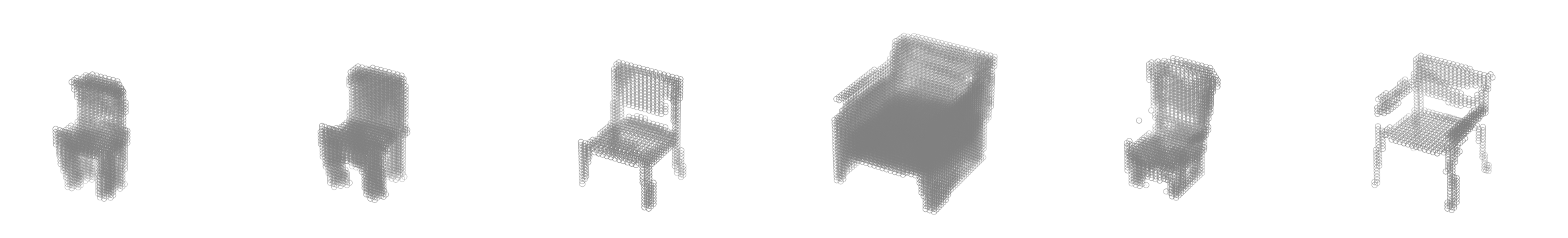
GASP    VaMoH   

GASP    VaMoH   

(b) ShapeNet

Figure 15: Comparison of generation quality of VaMoH and GASP at original resolution (top) and x2 resolution (bottom).

Original resolution Super-resolution

Functa    GASP    VaMoH   

Functa    GASP    VaMoH   

(a) Shapes3D

Original resolution Super-resolution

Functa    GASP    VaMoH   

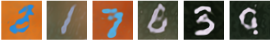
Functa    GASP    VaMoH   

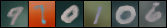
(b) PolyMNIST

Figure 17: Comparison of generation quality of VaMoH, Functa, and GASP at original resolution (top) and x2 resolution (bottom).

Original resolution

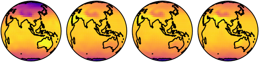
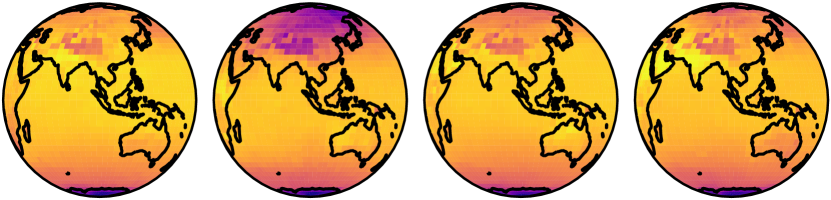
Functa    GASP    VaMoH   

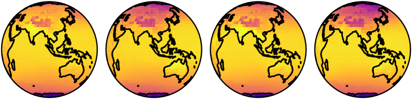
Super-resolution

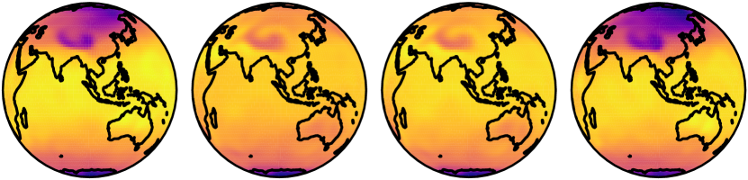
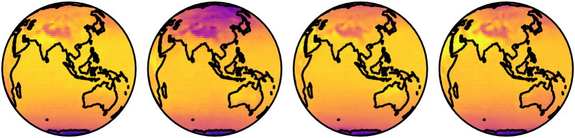
Functa    GASP    VaMoH   

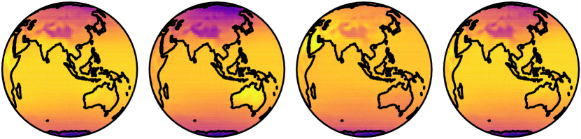
Figure 19: Comparison of generation quality of VaMoH, Functa, and GASP at original resolution (left) and x2 resolution (right).

B.3 Reconstruction

In this section, we provide a comprehensive set of figures demonstrating the capability of VaMoH in reconstructing data at both the original resolution and double the original resolution. Figure 21 and Figure 23 present the results for all datasets under examination. These figures reveal that VaMoH is able to produce high-quality reconstructions and super-reconstructions, with visual fidelity comparable or better to that of Functa, while requiring only a simple forward pass.

Furthermore, in Section 2, the Peak Signal to Noise Ratio (PSNR) is employed to evaluate the quality of the reconstruction, denoted as $\tilde{\bm{Y}}$, of an image, denoted as $\bm{Y}$. The computation of PSNR begins by calculating the root mean squared error (RMSE) and then PSNR itself as follows

$$\text{RMSE}=\sqrt{\frac{1}{D}\sum_{d}||\bm{y}_{d}-\tilde{\bm{y}_{d}}||_{2}^{2}},$$ (19)

$$\text{PSNR}=20\log\left(\frac{255}{\text{RMSE}}\right).$$ (20)

Table 5: Comparison of inference time (seconds) for super-reconstruction task of VaMoH and Functa. On the right-most two columns, we show the speed improvement of VaMoH compared to Functa (3) which is trained with 3 gradient steps as suggested in the original paper (Dupont et al., 2022a) and Functa (10) which is trained with 10 gradient steps to obtain the results of Functa depicted in Figures 21,23. Please note that these experiments are run on the same GPU device.

	Model Inference Time (secs)			Speed Improvement
Dataset	VaMoH	Functa (3)	Functa (10)	vs. Functa (3)	vs. Functa (10)
PolyMNIST	0.00455	0.01649	0.05109	x 3.62	x 11.23
Shapes3D	0.00544	0.01768	0.05489	x 3.25	x 10.09
CelebA HQ	0.00833	0.01729	0.05377	x 2.08	x 6.46
ERA5	0.00790	0.01997	0.06030	x 2.53	x 7.63
ShapeNet	0.01440	0.02089	0.06569	x 1.45	x 4.56

Ground truth

Reconstructions

Functa    VaMoH   

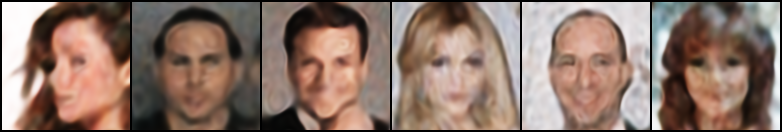
Functa    VaMoH   

Super-reconstructions

Figure 21: Comparison of reconstruction quality of VaMoH and Functa on ground truth images of CelebA HQ dataset at original resolution (top) and x2 resolution (bottom).

Ground truth

Reconstructions
Super-reconstructions

Functa    VaMoH   

Functa    VaMoH   

(a) ShapeNet

Ground truth

Reconstructions Super-reconstructions

Functa    VaMoH   

Functa    VaMoH   

(b) Shapes3D

Ground truth

Reconstructions Super-reconstructions

Functa    VaMoH   

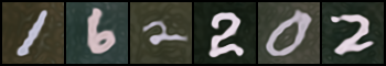
Functa    VaMoH   

(c) PolyMNIST

Ground truth

Reconstructions Super-reconstructions

Functa    VaMoH   

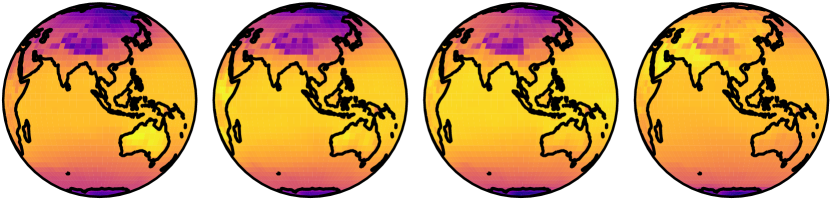
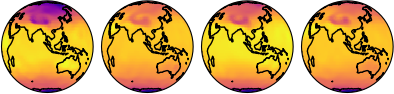
Functa    VaMoH   

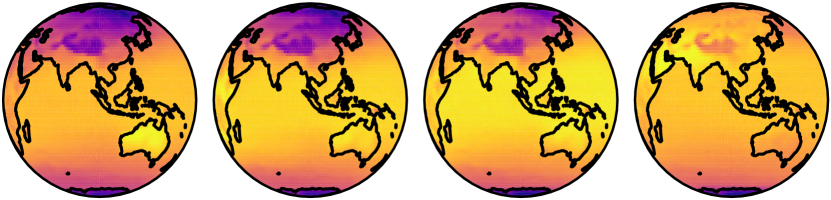
(d) ERA5

Figure 23: Comparison of reconstruction quality of VaMoH and Functa on ground truth data from the first samples of the test set at original and super-resolution.

B.4 Image completion

In this section, we provide qualitative results of VaMoH for various imputation tasks for different missingness patterns. As it is already highlighted in Section 3.3 and Section A.4, we use point dropout to increase the robustness of the encoder against missing data. In Figure 24, we provide results for image completion task on with different datasets.

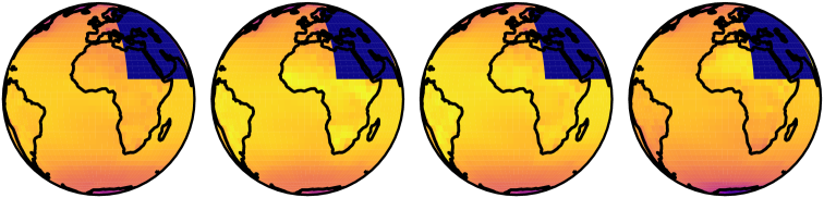
In    Recons.    In    Recons.    In    Recons.    In    Recons.   

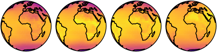
(a) Missing a patch (in-painting)

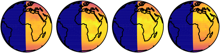
In    Recons.    In    Recons.    In    Recons.    In    Recons.   

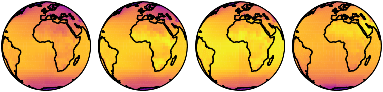
(b) Missing half of the image

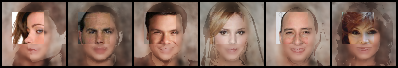
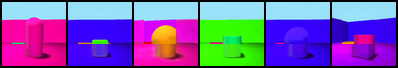
GT    Recons.    GT    Recons.    GT    Recons.   

(c) Image out-painting

Figure 24: Imputation of different amounts of missing parts using VaMoH. For each dataset, the top row shows the input (In) and the bottom row shows the reconstructed image (Recons.).

B.5 Entropy and Segmentation

In this section, we present figures that illustrate the contribution of each generator in the image reconstruction task. Specifically, we use entropy maps to visualize the uncertainty of the posterior probabilities of the categorical latent variable. A higher value in the entropy map indicates that the probabilities are more evenly distributed among the components for a given pixel, while a lower value suggests that a smaller number of components contribute to the reconstruction of that pixel. Additionally, we use segmentation maps to visualize the component with the highest probability per pixel, where different components are denoted by different colors. As an example, Figure 25(b) shows that there is a high degree of uncertainty among the components that are responsible for reconstructing the background in the CelebA HQ dataset. Conversely, for simpler datasets such as PolyMNIST, as shown in Figure 25(c), the components are able to differentiate between the object and background in the images. For Shapes3D dataset results presented in Figure 25(a), the uncertainty is lower in the Regions of Interest with high variations (borders), where only one of the components focuses on generating the shape and shadow of the object, as well as the perspective of the background wall. Thus, we provide evidence that meaningful interpretations can be obtained from our Mixture of HyperGenerators.

Test Recons Test Entropy Test Segmentation

(a) Shapes3D Test

Test Recons Test Entropy Test Segmentation

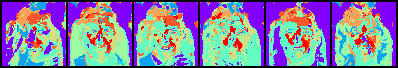
(b) CelebA HQ Test

Test Recons Test Entropy Test Segmentation

(c) PolyMNIST Test

Figure 25: Visualization of used components in mixture of generators of VaMoH for entropy (top) and segmentation (bottom) maps for Shapes3D, CelebA HQ, and PolyMNIST.

References

- Burgess & Kim (2018) Burgess, C. and Kim, H. 3d shapes dataset. https://github.com/deepmind/3dshapes-dataset/, 2018.
- Chang et al. (2015) Chang, A. X., Funkhouser, T., Guibas, L., Hanrahan, P., Huang, Q., Li, Z., Savarese, S., Savva, M., Song, S., Su, H., et al. Shapenet: An information-rich 3d model repository. arXiv preprint arXiv:1512.03012, 2015.
- Chen et al. (2017) Chen, X., Kingma, D. P., Salimans, T., Duan, Y., Dhariwal, P., Schulman, J., Sutskever, I., and Abbeel, P. Variational lossy autoencoder. In International Conference on Learning Representations, 2017. URL https://openreview.net/forum?id=BysvGP5ee.
- Chen & Zhang (2019) Chen, Z. and Zhang, H. Learning implicit fields for generative shape modeling. In Proceedings of the IEEE/CVF Conference on Computer Vision and Pattern Recognition, pp. 5939–5948, 2019.
- Cremer et al. (2018) Cremer, C., Li, X., and Duvenaud, D. Inference suboptimality in variational autoencoders. In International Conference on Machine Learning, pp. 1078–1086. PMLR, 2018.
- Dupont et al. (2022a) Dupont, E., Kim, H., Eslami, S. A., Rezende, D. J., and Rosenbaum, D. From data to functa: Your data point is a function and you can treat it like one. In International Conference on Machine Learning, pp. 5694–5725. PMLR, 2022a.
- Dupont et al. (2022b) Dupont, E., Teh, Y. W., and Doucet, A. Generative models as distributions of functions. In International Conference on Artificial Intelligence and Statistics, pp. 2989–3015. PMLR, 2022b.
- Gatopoulos & Tomczak (2021) Gatopoulos, I. and Tomczak, J. M. Self-supervised variational auto-encoders. Entropy, 23(6):747, 2021.
- Genova et al. (2019) Genova, K., Cole, F., Vlasic, D., Sarna, A., Freeman, W. T., and Funkhouser, T. Learning shape templates with structured implicit functions. In Proceedings of the IEEE/CVF International Conference on Computer Vision, pp. 7154–7164, 2019.
- Genova et al. (2020) Genova, K., Cole, F., Sud, A., Sarna, A., and Funkhouser, T. Local deep implicit functions for 3d shape. In Proceedings of the IEEE/CVF Conference on Computer Vision and Pattern Recognition, pp. 4857–4866, 2020.
- Grattarola & Vandergheynst (2022) Grattarola, D. and Vandergheynst, P. Generalised implicit neural representations. Advances in Neural Information Processing Systems, 2022.
- Ha (2016) Ha, D. Generating large images from latent vectors. blog.otoro.net, 2016. URL https://blog.otoro.net/2016/04/01/generating-large-images-from-latent-vectors/.
- Ha et al. (2017) Ha, D., Dai, A. M., and Le, Q. V. Hypernetworks. In International Conference on Learning Representations, 2017. URL https://openreview.net/forum?id=rkpACe1lx.
- Hao et al. (2022) Hao, Z., Mallya, A., Belongie, S., and Liu, M.-Y. Implicit neural representations with levels-of-experts. Advances in Neural Information Processing Systems, 2022.
- Hersbach et al. (2019) Hersbach, H., Bell, B., Berrisford, P., Biavati, G., Horányi, A., Muñoz Sabater, J., Nicolas, J., Peubey, C., Radu, R., Rozum, I., et al. Era5 monthly averaged data on single levels from 1979 to present. Copernicus Climate Change Service (C3S) Climate Data Store (CDS), 10:252–266, 2019.
- Heusel et al. (2017) Heusel, M., Ramsauer, H., Unterthiner, T., Nessler, B., and Hochreiter, S. Gans trained by a two time-scale update rule converge to a local nash equilibrium. Advances in neural information processing systems, 30, 2017.
- Hochreiter & Schmidhuber (1997) Hochreiter, S. and Schmidhuber, J. Long short-term memory. Neural computation, 9(8):1735–1780, 1997.
- Jabbar et al. (2020) Jabbar, A., Li, X., and Omar, B. A survey on generative adversarial networks: Variants, applications, and training. ACM Computing Surveys (CSUR), 54, 2020.
- Jiang et al. (2020) Jiang, C., Sud, A., Makadia, A., Huang, J., Nießner, M., Funkhouser, T., et al. Local implicit grid representations for 3d scenes. In Proceedings of the IEEE/CVF Conference on Computer Vision and Pattern Recognition, pp. 6001–6010, 2020.
- Karras et al. (2017) Karras, T., Aila, T., Laine, S., and Lehtinen, J. Progressive growing of gans for improved quality, stability, and variation. arXiv preprint arXiv:1710.10196, 2017.
- Kingma & Welling (2013) Kingma, D. P. and Welling, M. Auto-encoding variational bayes. arXiv preprint arXiv:1312.6114, 2013.
- Kingma et al. (2016) Kingma, D. P., Salimans, T., Jozefowicz, R., Chen, X., Sutskever, I., and Welling, M. Improved variational inference with inverse autoregressive flow. Advances in neural information processing systems, 29, 2016.
- Klushyn et al. (2019) Klushyn, A., Chen, N., Kurle, R., Cseke, B., and van der Smagt, P. Learning hierarchical priors in vaes. Advances in neural information processing systems, 32, 2019.
- Kynkäänniemi et al. (2019) Kynkäänniemi, T., Karras, T., Laine, S., Lehtinen, J., and Aila, T. Improved precision and recall metric for assessing generative models. Advances in Neural Information Processing Systems, 32, 2019.
- LeCun et al. (1995) LeCun, Y., Bengio, Y., et al. Convolutional networks for images, speech, and time series. The handbook of brain theory and neural networks, 3361(10):1995, 1995.
- Liu et al. (2015) Liu, Z., Luo, P., Wang, X., and Tang, X. Deep learning face attributes in the wild. In Proceedings of International Conference on Computer Vision (ICCV), December 2015.
- Loaiza-Ganem & Cunningham (2019) Loaiza-Ganem, G. and Cunningham, J. P. The continuous bernoulli: fixing a pervasive error in variational autoencoders. Advances in Neural Information Processing Systems, 32, 2019.
- Ma et al. (2020) Ma, C., Tschiatschek, S., Turner, R., Hernández-Lobato, J. M., and Zhang, C. Vaem: a deep generative model for heterogeneous mixed type data. Advances in Neural Information Processing Systems, 33:11237–11247, 2020.
- Maaløe et al. (2019) Maaløe, L., Fraccaro, M., Liévin, V., and Winther, O. Biva: A very deep hierarchy of latent variables for generative modeling. Advances in neural information processing systems, 32, 2019.
- Mescheder et al. (2019) Mescheder, L., Oechsle, M., Niemeyer, M., Nowozin, S., and Geiger, A. Occupancy networks: Learning 3d reconstruction in function space. In Proceedings of the IEEE/CVF conference on computer vision and pattern recognition, pp. 4460–4470, 2019.
- Mildenhall et al. (2021) Mildenhall, B., Srinivasan, P. P., Tancik, M., Barron, J. T., Ramamoorthi, R., and Ng, R. Nerf: Representing scenes as neural radiance fields for view synthesis. Communications of the ACM, 65(1):99–106, 2021.
- Nguyen et al. (2021) Nguyen, P., Tran, T., Gupta, S., Rana, S., Dam, H.-C., and Venkatesh, S. Variational hyper-encoding networks. In Joint European Conference on Machine Learning and Knowledge Discovery in Databases, pp. 100–115. Springer, 2021.
- Papamakarios et al. (2021) Papamakarios, G., Nalisnick, E. T., Rezende, D. J., Mohamed, S., and Lakshminarayanan, B. Normalizing flows for probabilistic modeling and inference. J. Mach. Learn. Res., 22(57):1–64, 2021.
- Peis et al. (2022) Peis, I., Ma, C., and Hernández-Lobato, J. M. Missing data imputation and acquisition with deep hierarchical models and hamiltonian monte carlo. In Advances in Neural Information Processing Systems 35, 2022.
- Rezende & Mohamed (2015) Rezende, D. and Mohamed, S. Variational inference with normalizing flows. In International Conference on Machine Learning, 2015.
- Rezende & Viola (2018) Rezende, D. J. and Viola, F. Taming vaes. arXiv preprint arXiv:1810.00597, 2018.
- Rezende et al. (2014) Rezende, D. J., Mohamed, S., and Wierstra, D. Stochastic backpropagation and approximate inference in deep generative models. In International conference on machine learning, pp. 1278–1286. PMLR, 2014.
- Rodríguez-Santana et al. (2022) Rodríguez-Santana, S., Zaldivar, B., and Hernandez-Lobato, D. Function-space inference with sparse implicit processes. In International Conference on Machine Learning, pp. 18723–18740. PMLR, 2022.
- Salimans et al. (2017) Salimans, T., Karpathy, A., Chen, X., and Kingma, D. P. Pixelcnn++: Improving the pixelcnn with discretized logistic mixture likelihood and other modifications. arXiv preprint arXiv:1701.05517, 2017.
- Simkus et al. (2021) Simkus, V., Rhodes, B., and Gutmann, M. U. Variational gibbs inference for statistical model estimation from incomplete data. arXiv preprint arXiv:2111.13180, 2021.
- Simonyan & Zisserman (2014) Simonyan, K. and Zisserman, A. Very deep convolutional networks for large-scale image recognition. arXiv preprint arXiv:1409.1556, 2014.
- Sitzmann et al. (2019) Sitzmann, V., Zollhöfer, M., and Wetzstein, G. Scene representation networks: Continuous 3d-structure-aware neural scene representations. Advances in Neural Information Processing Systems, 32, 2019.
- Sitzmann et al. (2020) Sitzmann, V., Martel, J., Bergman, A., Lindell, D., and Wetzstein, G. Implicit neural representations with periodic activation functions. Advances in Neural Information Processing Systems, 33:7462–7473, 2020.
- Stanley (2007) Stanley, K. O. Compositional pattern producing networks: A novel abstraction of development. Genetic programming and evolvable machines, 8(2):131–162, 2007.
- Tancik et al. (2020) Tancik, M., Srinivasan, P., Mildenhall, B., Fridovich-Keil, S., Raghavan, N., Singhal, U., Ramamoorthi, R., Barron, J., and Ng, R. Fourier features let networks learn high frequency functions in low dimensional domains. In Larochelle, H., Ranzato, M., Hadsell, R., Balcan, M., and Lin, H. (eds.), Advances in Neural Information Processing Systems, volume 33, pp. 7537–7547. Curran Associates, Inc., 2020. URL https://proceedings.neurips.cc/paper/2020/file/55053683268957697aa39fba6f231c68-Paper.pdf.
- Tomczak & Welling (2018) Tomczak, J. and Welling, M. Vae with a vampprior. In International Conference on Artificial Intelligence and Statistics, pp. 1214–1223. PMLR, 2018.
- Wu et al. (2019) Wu, W., Qi, Z., and Fuxin, L. Pointconv: Deep convolutional networks on 3d point clouds. In Proceedings of the IEEE/CVF Conference on Computer Vision and Pattern Recognition, pp. 9621–9630, 2019.
- Zeng et al. (2022) Zeng, X., Vahdat, A., Williams, F., Gojcic, Z., Litany, O., Fidler, S., and Kreis, K. Lion: Latent point diffusion models for 3d shape generation. In Advances in Neural Information Processing Systems (NeurIPS), 2022.
- Zhang et al. (2018) Zhang, C., Bütepage, J., Kjellström, H., and Mandt, S. Advances in variational inference. IEEE transactions on pattern analysis and machine intelligence, 41(8):2008–2026, 2018.