Reliability Assurance for Deep Neural Network Architectures Against Numerical Defects

Abstract

With the widespread deployment of deep neural networks (DNNs), ensuring the reliability of DNN-based systems is of great importance. Serious reliability issues such as system failures can be caused by numerical defects, one of the most frequent defects in DNNs. To assure high reliability against numerical defects, in this paper, we propose the RANUM approach including novel techniques for three reliability assurance tasks: detection of potential numerical defects, confirmation of potential-defect feasibility, and suggestion of defect fixes. To the best of our knowledge, RANUM is the first approach that confirms potential-defect feasibility with failure-exhibiting tests and suggests fixes automatically. Extensive experiments on the benchmarks of 63 real-world DNN architectures show that RANUM outperforms state-of-the-art approaches across the three reliability assurance tasks. In addition, when the RANUM-generated fixes are compared with developers’ fixes on open-source projects, in 37 out of 40 cases, RANUM-generated fixes are equivalent to or even better than human fixes.

I Introduction

Deep Neural Networks (DNNs) are successfully deployed and show remarkable performance in many challenging applications, including facial recognition [21, 56], game playing [38], and code completion [20, 4]. To develop and deploy DNNs, one needs to attain a DNN architecture, which is usually encoded by program code as the example shown in Figure 2. First, for training, the user executes the program with the architecture on the given training/validation data, attains the model weights, and stores them in a weight file. The architecture along with the weights is named a model. Then, for inference, the user loads the weight file to CPU/GPU memory or AI chips, executes the same program with the given inference sample and weights as arguments, and gets the model prediction result as the program output. With the wide deployment of DNN models (resulted from training DNN architectures), reliability issues of DNN-based systems have become a serious concern, where malfunctioning DNN-based systems have led to serious consequences such as fatal traffic accidents [24].

To assure the reliability of DNN-based systems, it is highly critical to detect and fix numerical defects for two main reasons. First, numerical defects widely exist in DNN-based systems. For example, in the DeepStability database [14], over 250 defects are identified in deep learning (DL) algorithms where over 60% of them are numerical defects. Moreover, since numerical defects exist at the architecture level, any model using the architecture naturally inherits these defects. Second, numerical defects can result in serious consequences. Once numerical defects (such as divide-by-zero) are exposed, the faulty DNN model will output NaN or INF instead of producing any meaningful prediction, resulting in numerical failures and system crashes [60, 58]. Thus, numerical defects hinder the application of DNNs in scenarios with high reliability and availability requirements such as threat monitoring in cybersecurity [33] and cloud system controlling [36, 13].

Figure 1: Workflow for reliability assurance against numerical defects in DNN architectures. The left-hand side shows three tasks and the right-hand side shows corresponding examples. RANUM supports all the three tasks, and is the first automatic approach for system test generation and fix suggestion.

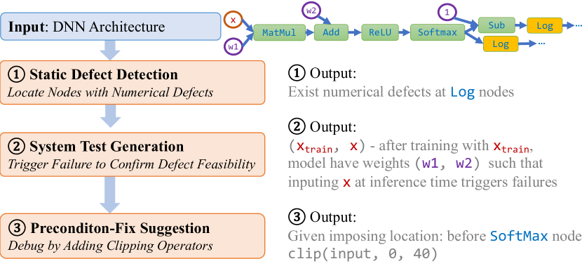
To address numerical defects in DNN architectures in an actionable manner [53], in this paper, we propose a workflow of reliability assurance (as shown in Figure 1), consisting of three tasks: potential-defect detection, feasibility confirmation, and fix suggestion, along with our proposed approach to support all these three tasks.

Potential-Defect Detection. In this task, we detect all potential numerical defects in a DNN architecture, with a focus on operators with numerical defects (in short as defective operators) that potentially exhibit inference-phase numerical failures for two main reasons, following the literature [61, 54]. First, these defective operators can be exposed after the model is deployed and thus are more devastating than those that potentially exhibit training-phase numerical failures [27, 61]. Second, a defective operator that potentially exhibits training-phase numerical failures can usually be triggered to exhibit inference-phase numerical failures, thus also being detected by our task. For example, the type of training-phase NaN gradient failures is caused by an operator’s input that leads to invalid derivatives, and this input also triggers failures in the inference phase [54].

Feasibility Confirmation. In this task, we confirm the feasibility of these potential numerical defects by generating failure-exhibiting system tests. As shown in Figure 1, a system test is a tuple of training example ${\bm{x}}_{\mathsf{train}}$ and inference example ${\bm{x}}$ such that after the training example is used to train the architecture under consideration, applying the resulting model on the inference example exhibits a numerical failure.

Fix Suggestion. In this task, we fix a feasible numerical defect. To determine the fix form, we have inspected the developers’ fixes of the numerical defects collected by Zhang et al. [60] by looking at follow-up Stack Overflow posts or GitHub commits. Among the 13 numerical defects whose fixes can be located, 12 fixes can be viewed as explicitly or implicitly imposing interval preconditions on different locations, such as after inputs or weights are loaded and before defective operators are invoked. Thus, imposing an interval precondition, e.g., by clipping (i.e., chopping off the input parts that exceed the specified input range) the input for defective operator(s), is an effective and common strategy for fixing a numerical defect. Given a location (i.e., one related to an operator, input, or weight where users prefer to impose a fix), we suggest a fix for the numerical defect under consideration.

To support all the three tasks of the reliability assurance process against DNN numerical defects, we propose the RANUM approach in this paper.

For task \raisebox{-0.9pt}{1}⃝ and task \raisebox{-0.9pt}{2}⃝a, which are already supported by two existing tools (DEBAR [61] and GRIST [54]), RANUM introduces novel extensions and optimizations that substantially improve the effectiveness and efficiency. (1) DEBAR [61] is the state-of-the-art tool for potential-defect detection; however, DEBAR can handle only static computational graphs and does not support widely used dynamic graphs in PyTorch programs [28]. RANUM supports dynamic graphs thanks to our novel technique of backward fine-grained node labeling. (2) GRIST [54] is the state-of-the-art tool for generating failure-exhibiting unit tests to confirm potential-defect feasibility; however, GRIST conducts gradient back-propagation by using the original inference input and weights as the starting point. Recent studies [23, 8] on DNN adversarial attacks suggest that using a randomized input as the starting point leads to stronger attacks than using the original input. Taking this observation, we combine gradient back-propagation with random initialization in RANUM.

For task \raisebox{-0.9pt}{2}⃝ and task \raisebox{-0.9pt}{3}⃝, which are not supported by any existing tool, RANUM is the first automatic approach for them.

For feasibility confirmation, RANUM is the first approach that generates failure-exhibiting system tests that contain training examples. Doing so is a major step further from the existing GRIST tool, which generates failure-exhibiting unit tests ignoring the practicality of generated model weights. Given that in practice model weights are determined by training examples, we propose the technique of two-step generation for this task. First, we generate a failure-exhibiting unit test. Second, we generate a training example that leads to the model weights in the unit test when used for training. For the second step, we extend the deep-leakage-from-gradient (DLG) attack [63] by incorporating the straight-through gradient estimator [3].

For fix suggestion, RANUM is the first automatic approach. RANUM is based on the novel technique of abstraction optimization. We observe that a defect fix in practice is typically imposing interval clipping on some operators such that each later-executed operator (including those defective ones) can never exhibit numerical failures. Therefore, we propose the novel technique of abstraction optimization to “deviate away” the input range of a defective operator from the invalid range, falling in which can cause numerical failures.

For RANUM, we implement a tool and evaluate it on the benchmarks [54] of 63 real-world DNN architectures containing 79 real numerical defects; these benchmarks are the largest benchmarks of DNN numerical defects to the best of our knowledge. The evaluation results show that RANUM is both effective and efficient in all the three tasks for DNN reliability assurance. (1) For potential-defect detection, RANUM detects $>$60% more true defects than the state-of-the-art DEBAR approach. (2) For feasibility confirmation, RANUM generates failure-exhibiting unit tests to confirm potential numerical defects in the benchmarks with 100% success rate; in contrast, with the much higher time cost (17.32X), the state-of-the-art GRIST approach generates unit tests to confirm defects with 96.96% success rate. More importantly, for the first time, RANUM generates failure-exhibiting system tests that confirm defects (with 92.78% success rate). (3) For fix suggestion, RANUM proposes fix suggestions for numerical defects with 100% success rate. In addition, when the RANUM-generated fixes are compared with developers’ fixes on open-source projects, in 37 out of 40 cases, RANUM-generated fixes are equivalent to or even better than human fixes.

This paper makes the following main contributions:

• We formulate the reliability assurance problem for DNN architectures against numerical defects and elaborate on three important tasks for this problem.

• We propose RANUM—the first automatic approach that solves all these three tasks. RANUM includes three novel techniques (backward fine-grained node labeling, two-step test generation, and abstraction optimization) and solves system test generation and fix suggestion for the first time.

• We implement RANUM and apply it on 63 real-world DNN architectures, showing the high effectiveness and efficiency of RANUM compared to both the state-of-the-art approaches and developers’ fixes.

II Background and Approach Overview

In this section, we introduce the background of DNN numerical defects and failures, and then give an overview of the RANUM approach with a running example.

II-A Background

Figure 2: A DL program snippet that defines a linear regression model from benchmarks of real-world numerical defects (Case 2a in [54]).

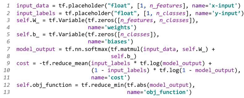
DL developers define the DNN architecture with code using modern DL libraries such as PyTorch [28] and TensorFlow [1]. The DNN architecture can be expressed by a computational graph. Figures 2 and 3 depict a real-world example. Specifically, the DNN architecture in a DL program can be automatically converted to an ONNX-format computational graph [43].

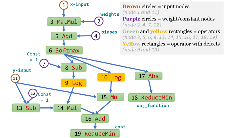
The computational graph can be viewed as a Directed Acyclic Graph (DAG): ${\mathcal{G}}=\langle{\mathcal{V}},{\mathcal{E}}\rangle$, where ${\mathcal{V}}$ and ${\mathcal{E}}$ are sets of nodes and edges, respectively. We call nodes with zero in-degree as initial nodes, which correspond to input, weight, or constant nodes. Initial nodes provide concrete data for the DNN models resulted from training the DNN architecture. The data from each node is formatted as a tensor, i.e., a multidimensional array, with a specified data type and array shape annotated alongside the node definition. We call nodes with positive in-degree as internal nodes, which correspond to concrete operators, such as matrix multiplication (MatMul) and addition (Add). During model training, the model weights, i.e., data from weight nodes, are generated by the training algorithm. Then, in the deployment phase (i.e., model inference), with these trained weights and a user-specified input named inference example, the output of each operator is computed in the topological order. The output of some specific node is used as the prediction result.

We let ${\bm{x}}$ and ${\bm{w}}$ denote the concatenation of data from all input nodes and data from all weight nodes, respectively. For example, in Figure 3, ${\bm{x}}$ concatenates data from nodes 1 and 11; and ${\bm{w}}$ concatenates data from nodes 2 and 4. Given specific ${\bm{x}}$ and ${\bm{w}}$, the input and output for each node are deterministic. We use $f^{\mathsf{in}}_{n}({\bm{x}};{\bm{w}})$ and $f^{\mathsf{out}}_{n}({\bm{x}};{\bm{w}})$ to express input and output data of node $n$, respectively, given ${\bm{x}}$ and ${\bm{w}}$.

Numerical Defects in DNN Architecture. We focus on inference-phase numerical defects. These defects lead to numerical failures when specific operators receive inputs within invalid ranges so that the operators output NaN or INF.

Definition 1.

For the given computational graph ${\mathcal{G}}=\langle{\mathcal{V}},{\mathcal{E}}\rangle$, if there is a node $n_{0}\in{\mathcal{V}}$, such that there exists a valid input and valid weights that can let the input of node $n_{0}$ fall within the invalid range, we say there is a numerical defect at node $n_{0}$.

Formally, $$\exists{\bm{x}}_{0}\in{\mathcal{X}}_{\mathsf{valid}},{\bm{w}}_{0}\in{\mathcal{W}}_{\mathsf{valid}},f^{\mathsf{in}}_{n_{0}}({\bm{x}}_{0};{\bm{w}}_{0})\in{\mathcal{I}}_{n_{0},\mathsf{invalid}}$$

$$\Longrightarrow \text{$\exists$ numerical defect at node $n_{0}$}.$$

In the definition, ${\mathcal{X}}_{\mathsf{valid}}$ and ${\mathcal{W}}_{\mathsf{valid}}$ are valid input range and weight range, respectively, which are clear given the deployed scenario. For example, ImageNet Resnet50 models have valid input range ${\mathcal{X}}_{\mathsf{valid}}=[0,1]^{3\times 224\times 224}$ since image pixel intensities are within $[0,1]$, and valid weight range ${\mathcal{W}}_{\mathsf{valid}}=[-1,1]^{p}$ where $p$ is the number of parameters since weights of well-trained Resnet50 models are typically within $[-1,1]$. The invalid range ${\mathcal{I}}_{n_{0},\mathsf{invalid}}$ is determined by $n_{0}$’s operator type with detailed definitions in Section -B. For example, for the Log operator, the invalid range ${\mathcal{I}}_{n_{0},\mathsf{invalid}}=(-\infty,U_{\min})$ where $U_{\min}$ is the smallest positive number of a tensor’s data type.

II-B Approach Overview

Figure 3: Computational graph encoded by the snippet in Figure 2.

Figure 4: Overview of the RANUM approach. The output of RANUM indicates confirmation and manifestation of numerical defects (that can be feasibly exposed at the system level) for a given DNN architecture and effective fixes for the architecture’s confirmed defects.

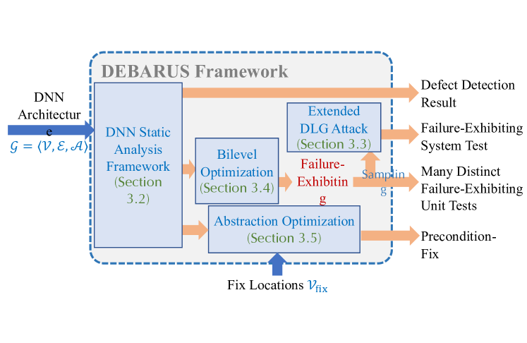
In Figure 4, we show the overview structure of the RANUM approach. RANUM takes a DNN architecture as the input. Note that although RANUM is mainly designed and illustrated for a DNN architecture, the RANUM approach can also be directly applied to general neural network architectures since they can also be expressed by computational graphs. First, the DNN static analysis framework (task \raisebox{-0.9pt}{1}⃝ in Figure 1) in RANUM detects all potential numerical defects in the architecture. Second, the two-step test generation component (task \raisebox{-0.9pt}{2}⃝ in Figure 1), including unit test generation and training example generation, confirms the feasibility of these potential numerical defects. Third, the abstraction optimization component (task \raisebox{-0.9pt}{3}⃝ in Figure 1) takes the input/output abstractions produced by the DNN static analysis framework along with the user-specified fix locations, and produces preconditions to fix the confirmed defects.

We next go through the whole process in detail taking the DNN architecture shown in Figure 3 as a running example.

Task \raisebox{-0.9pt}{1}⃝: Potential-Defect Detection via Static Analysis

The DNN static analysis framework within RANUM first computes the numerical intervals of possible inputs and outputs for all nodes within the given DNN architecture, and then flags any nodes whose input intervals overlap with their invalid ranges as nodes with potential numerical defects.

In Figure 3, suppose that the user-specified input x-input (node 1) is within (elementwise, same below) range $[(-10,-10)^{\scriptscriptstyle\mathsf{T}},(10,10)^{\scriptscriptstyle\mathsf{T}}]$; weights (node 2) are within range ${\scriptsize[\begin{bmatrix}-10&-10\\ -10&-10\end{bmatrix},\begin{bmatrix}10&10\\ 10&10\end{bmatrix}]}$; and biases (node 4) are within range $[(-10,-10)^{\scriptscriptstyle\mathsf{T}},(10,10)^{\scriptscriptstyle\mathsf{T}}]$. Our DNN static analysis framework computes these interval abstractions for node inputs:

1. Node 5 (after MatMul): $[(-200,-200)^{\scriptscriptstyle\mathsf{T}},(200,200)^{\scriptscriptstyle\mathsf{T}}]$;

2. Node 6 (after Add): $[(-210,-210)^{\scriptscriptstyle\mathsf{T}},(210,210)^{\scriptscriptstyle\mathsf{T}}]$;

3. Node 8 (after Softmax in float32): $[(0,0)^{\scriptscriptstyle\mathsf{T}},(1,1)^{\scriptscriptstyle\mathsf{T}}]$;

4. Node 9 (after Sub of $[1,1]$ and node 8), 10: $[(0,0)^{\scriptscriptstyle\mathsf{T}},(1,1)^{\scriptscriptstyle\mathsf{T}}]$.

Since nodes 9 and 10 use the Log operator whose invalid input range $(-\infty,U_{\min})$ overlaps with their input range $[(0,0)^{\scriptscriptstyle\mathsf{T}},(1,1)^{\scriptscriptstyle\mathsf{T}}]$, we flag nodes 9 and 10 as potential numerical defects.

This static analysis process follows the state-of-the-art DEBAR tool [61]. However, we extend DEBAR with a novel technique named backward fine-grained node labeling. This technique detects all nodes that require fine-grained abstractions, e.g., nodes that determine the control flow in a dynamic graph. For these nodes, we apply interval abstractions with the finest granularity to reduce control flow ambiguity. For other nodes, we let some neighboring elements share the same interval abstraction to improve efficiency while preserving tightness. As a result, the static analysis in RANUM has high efficiency and supports much more DNN operators including dynamic control-flow operators like Loop than DEBAR does.

Task \raisebox{-0.9pt}{2}⃝: Feasibility Confirmation via Two-Step Test Generation

Given nodes that contain potential numerical defects (nodes 9 and 10 in our example), we generate failure-exhibiting system tests to confirm their feasibility. A failure-exhibiting system test is a tuple $\langle{\bm{x}}_{\mathsf{train}},{\bm{x}}_{\mathsf{infer}}\rangle$, such that after training the architecture with the training example ${\bm{x}}_{\mathsf{train}}$, with the trained model weights ${\bm{w}}_{\mathsf{infer}}$, the inference input ${\bm{x}}_{\mathsf{infer}}$ triggers a numerical failure. The name “system test” is inspired by traditional software testing, where we test the method sequence (m = train(${\bm{x}}_{\mathsf{train}}$); m.infer(${\bm{x}}_{\mathsf{infer}}$)). In contrast, GRIST [54] generates model weights ${\bm{w}}_{\mathsf{infer}}$ along with inference input ${\bm{x}}_{\mathsf{infer}}$ that tests only the inference method m.infer(), and the weights may be infeasible from training. Hence, we view the GRIST-generated tuple $\langle{\bm{w}}_{\mathsf{infer}},{\bm{x}}_{\mathsf{infer}}\rangle$ as a “unit test”.

We propose a two-step test generation technique to generate failure-exhibiting system tests.

Step a: Generate failure-exhibiting unit test $\langle{\bm{w}}_{\mathsf{infer}},{\bm{x}}_{\mathsf{infer}}\rangle$. The state-of-the-art GRIST tool supports this step. However, GRIST solely relies on gradient back-propagation, which is relatively inefficient. In RANUM, we augment GRIST by combining its gradient back-propagation with random initialization inspired by recent research on DNN adversarial attacks [8, 23]. As a result, RANUM achieves 17.32X speedup with 100% success rate. Back to the running example in Figure 3, RANUM can generate ${\scriptsize\begin{bmatrix}5&-5\\ -5&5\end{bmatrix}}$ for node 2 and $(0.9,-0.9)^{\scriptscriptstyle\mathsf{T}}$ for node 4 as model weights ${\bm{w}}_{\mathsf{infer}}$; and $(10,-10)^{\scriptscriptstyle\mathsf{T}}$ for node 1 and $(1,0)^{\scriptscriptstyle\mathsf{T}}$ for node 11 as the inference input ${\bm{x}}_{\mathsf{infer}}$. Such ${\bm{w}}_{\mathsf{infer}}$ and ${\bm{x}}_{\mathsf{infer}}$ induce input $(0,1)^{\scriptscriptstyle\mathsf{T}}$ and $(1,0)^{\scriptscriptstyle\mathsf{T}}$ for nodes 9 and 10, respectively. Since both nodes 9 and 10 use the log operator and $\log 0$ is undefined, both nodes 9 and 10 trigger numerical failures.

Step b: Generate training example ${\bm{x}}_{\mathsf{train}}$ that achieves model weights ${\bm{w}}_{\mathsf{infer}}$. To the best of our knowledge, there is no automatic approach for this task yet. RANUM provides support for this task based on our extension of DLG attack [63]. The DLG attack is originally designed for recovering the training data from training-phase gradient leakage. Here, we figure out the required training gradients to trigger the numerical failure at the inference phase and then leverage the DLG attack to generate ${\bm{x}}_{\mathsf{train}}$ that leads to such training gradients. Specifically, many DNN architectures contain operators (such as ReLU) on which DLG attack is hard to operate [35]. We combine straight-through estimator [3] to provide proxy gradients and bypass this barrier. Back to the running example in Figure 3, supposing that the initial weights are ${\scriptsize\begin{bmatrix}-0.1&0.1\\ 0.1&-0.1\end{bmatrix}}$ for node 2 and $(0,0)^{\scriptscriptstyle\mathsf{T}}$ for node 4, RANUM can generate training example ${\bm{x}}_{\mathsf{train}}$ composed of $(5.635,-5.635)^{\scriptscriptstyle\mathsf{T}}$ for node 1 and $(1,0)^{\scriptscriptstyle\mathsf{T}}$ for node 11, such that one-step training with learning rate 1 on this example leads to ${\bm{w}}_{\mathsf{infer}}$. Combining ${\bm{x}}_{\mathsf{train}}$ from this step with ${\bm{x}}_{\mathsf{infer}}$ from step a, we obtain a failure-exhibiting system test that confirms the feasibility of potential defects in nodes 9 and 10.

Task \raisebox{-0.9pt}{3}⃝: Fix Suggestion via Abstract Optimization

In this task, we suggest fixes for the confirmed numerical defects. RANUM is the first approach for this task to our knowledge.

The user may prefer different fix locations, which correspond to a user-specified set of nodes ${\mathcal{V}}_{\mathsf{fix}}\subseteq{\mathcal{V}}$ to impose the fix. For example, if the fix method is clipping the inference input, ${\mathcal{V}}_{\mathsf{fix}}$ are input nodes (e.g., nodes 1, 11 in Figure 3); if the fix method is clipping the model weights during training, ${\mathcal{V}}_{\mathsf{fix}}$ are weight nodes (e.g., nodes 2, 4 in Figure 3); if the fix method is clipping before the defective operator, ${\mathcal{V}}_{\mathsf{fix}}$ are nodes with numerical defects (e.g., nodes 9, 10 in Figure 3).

According to the empirical study of developers’ fixes in Section I, 12 out of 13 defects are fixed by imposing interval preconditions for clipping the inputs of ${\mathcal{V}}_{\mathsf{fix}}$. Hence, we suggest interval precondition, which is interval constraint ${\bm{l}}_{n}\leq f^{\mathsf{in}}_{n}({\bm{x}};{\bm{w}})\leq{\bm{u}}_{n}$ for nodes $n\in{\mathcal{V}}_{\mathsf{fix}}$, as the defect fix in this paper. A fix should satisfy that, when these constraints $\bigwedge_{n\in{\mathcal{V}}_{\mathsf{fix}}}({\bm{l}}_{n}\leq f^{\mathsf{in}}_{n}({\bm{x}};{\bm{w}})\leq{\bm{u}}_{n})$ are imposed, the input of any node in the computational graph should always be valid, i.e., $f^{\mathsf{in}}_{n_{0}}({\bm{x}};{\bm{w}})\notin{\mathcal{I}}_{n_{0},\mathsf{invalid}},\forall n_{0}\in{\mathcal{V}}$.

In RANUM, we formulate the fix suggestion task as a constrained optimization problem, taking the endpoints of interval abstractions for nodes in ${\mathcal{V}}_{\mathsf{fix}}$ as optimizable variables. We then propose the novel technique of abstraction optimization to solve this constrained optimization problem. Back to the Figure 3 example, if users plan to impose a fix on inference input, RANUM can suggest the fix $-1\leq$ x-input $\leq 1$; if users plan to impose a fix on nodes with numerical defects, RANUM can suggest the fix $10^{-38}\leq$ node 9 & node 10.input $\leq+\infty$.

III The RANUM Approach

In this section, we introduce the three novel techniques in RANUM: backward fine-grained node labeling in Section III-A; two-step test generation in Section III-B; and abstraction optimization in Section III-C.

III-A DNN Static Analysis Framework with Backward Fine-Grained Node Labeling for Potential-Defect Detection

RANUM contains a static analysis framework to enable potential-defect detection and support downstream tasks as shown in Figure 4. Given a DNN architecture and valid ranges for input and weight nodes, the static analysis framework computes interval abstractions for possible inputs and outputs of each node. As a result, we can check whether an overlap exists between the interval abstraction and invalid input ranges for all nodes in the graph to detect potential numerical defects. Then, the defective nodes are fed into the two-step test generation component to confirm the feasibility of potential defects; and the differentiable abstractions are fed into the abstract optimization component to produce fixes.

Formally, for given valid ranges of inference input and model weights, namely ${\mathcal{X}}$ and ${\mathcal{W}}$, for each node $n\in{\mathcal{V}}$, our framework computes sound input interval abstraction $[{\bm{l}}_{n},{\bm{u}}_{n}]:=\{{\bm{x}}:{\bm{l}}_{n}\leq{\bm{x}}\leq{\bm{u}}_{n}\}$ such that $[{\bm{l}}_{n},{\bm{u}}_{n}]$ always captures all possible inputs of the node: $[{\bm{l}}_{n},{\bm{u}}_{n}]\supseteq\{f^{\mathsf{in}}_{n}({\bm{x}},{\bm{w}}):{\bm{x}}\in{\mathcal{X}},{\bm{w}}\in{\mathcal{W}}\}$. We also compute output interval abstractions similarly.

Compared with traditional analysis tools for numerical software [10, 39], RANUM’s static analysis framework designs abstractions for DNN primitives operating on multi-dimensional tensors that are not supported by traditional tools. Compared with the state-of-the-art DEBAR tool [61], RANUM uses the same abstraction domain (interval domain with tensor partitioning), but incorporates a novel technique (backward fine-grained node labeling) to improve abstraction precision and support a wider range of DNN architectures.

Abstract Domain: Interval with Tensor Partitioning. Following DEBAR’s design, we use the interval with tensor partitioning [61] as the abstraction domain. This abstraction domain partitions a tensor into multiple subblocks and shares the interval abstractions at the block level instead of imposing abstractions at the element level. Therefore, we can compute the abstraction of a smaller size than the original tensor to improve efficiency.

Our Technique: Backward Fine-Grained Node Labeling

The interval domain with tensor partitioning provides a degree of freedom in terms of the partition granularity, i.e., we can choose the subblock size for each node’s abstraction. When the finest granularity, i.e., elementwise abstraction, is chosen, the abstraction interval is the most concrete. When the coarsest granularity (i.e., one scalar to summarize the node tensor) is chosen, the abstraction saves the most space and computational cost but loses much precision.

Example. Suppose that the possible input range of a node is $([-1,0],[0,1],[1,2],[-1,0])$, where each interval $[l,u]$ specifies the range of corresponding elements in the four-dimensional vector. If we choose the finest granularity, we use $[{\bm{l}}_{n},{\bm{u}}_{n}]=[(-1,0,1,-1),(0,1,2,0)]$ as the input range abstraction. If we choose the coarsest granularity, we use $[{\bm{l}}_{n},{\bm{u}}_{n}]=[-1,2]$ as the abstraction where the same interval is shared for all elements. As we can see, finer granularity provides tighter abstraction at the expense of larger computational and space costs.

In DEBAR, the coarsest granularity is used by default for most operators. However, we find that using the finest instead of the coarsest granularity for some nodes is more beneficial for overall abstraction preciseness. For example, the control-flow operators (e.g., Loop) benefit from concrete execution to determine the exact control flow in the dynamic graph, and the indexing operators (e.g., Slice) and shaping operators (e.g., Reshape) benefit from explicit indexers and shapes to precisely infer the output range. Hence, we propose to use the finest granularity for some nodes (namely fine-grained requiring operators) while the coarsest granularity for other nodes during static analysis.

To benefit from the finest granularity abstraction for required nodes, typically, all of their preceding nodes also need the finest granularity. Otherwise, the over-approximated intervals from preceding nodes will be propagated to the required nodes, making the finest abstraction for the required nodes useless. To solve this problem, in RANUM, we back-propagate “fine-grained” labels from these fine-grained requiring nodes to initial nodes by topologically sorting the graph with inverted edges, and then apply the finest granularity abstractions on all labeled nodes. In practice, we find that this strategy eliminates the control-flow ambiguity and indexing ambiguity with little loss of efficiency. As a result, RANUM supports all dynamic graphs (which are not supported by DEBAR) that comprise 39.2% of the benchmarks proposed by Yan et al. [54].

Furthermore, when preceding nodes use finer-grain abstraction granularity, the subsequent nodes should preserve such fine granularity to preserve the analysis preciseness. Principally, the choice of abstraction granularity should satisfy both tightness (bearing no precision loss compared to elementwise interval abstraction) and minimality (using the minimum number of partitions for high efficiency). To realize these principles, we dynamically determine a node’s abstraction granularity based on the granularity of preceding nodes. The abstraction design for some operators is non-trivial. Omitted details (formulation, illustration, and proofs) about the static analysis framework are in Section -C.

In summary, the whole static analysis process consists of three steps. (1) Determine the tensor partition granularity of all initial nodes by our technique of backward fine-grained node labeling. (2) Sort all nodes in the graph in the topological order. (3) Apply corresponding abstraction computation algorithms for each node based on the preceding node’s abstractions. The key insight behind the design of our static analysis framework is the strategic granularity selection for tensor abstraction, maintaining both high efficiency (by selecting the coarse granularity for data-intensive nodes) and high precision (by selecting the fine granularity for some critical nodes, such as nodes with control-flow, indexing, and shaping operators).

III-B Two-Step Test Generation for Feasibility Confirmation

RANUM generates failure-exhibiting system tests for the given DNN to confirm the feasibility of potential numerical defects. Here, we take the DNN architecture as the input. From the static analysis framework, we obtain a list of nodes that have potential numerical defects. For each node $n_{0}$ within the list, we apply our technique of two-step test generation to produce a failure-exhibiting system test $t_{\mathsf{sys}}=\langle{\bm{x}}_{\mathsf{train}},{\bm{x}}_{\mathsf{infer}}\rangle$ as the output. According to Section II-B, the test should satisfy that after the architecture is trained with ${\bm{x}}_{\mathsf{train}}$, entering ${\bm{x}}_{\mathsf{infer}}$ in the inference phase results in a numerical failure.

We propose the novel technique of two-step test generation: first, generate failure-exhibiting unit test $\langle{\bm{w}}_{\mathsf{infer}},{\bm{x}}_{\mathsf{infer}}\rangle$; then, generate training example ${\bm{x}}_{\mathsf{train}}$ that leads model weights to be close to ${\bm{w}}_{\mathsf{infer}}$ after training.

Step a: Unit Test Generation

As sketched in Section II-B, we strengthen the state-of-the-art unit test generation approach, GRIST [54], by combining it with random initialization to complete this step. Specifically, GRIST leverages the gradients of the defective node’s input with respect to the inference input and weights to iteratively update the inference input and weights to generate failure-exhibiting unit tests. However, GRIST always conducts updates from the existing inference input and weights, suffering from local minima problem [23]. Instead, motivated by DNN adversarial attack literature [23, 45], a sufficient number of random starts help find global minima effectively. Hence, in RANUM, we first conduct uniform sampling 100 times for both the inference input and weights to trigger the numerical failure. If no failure is triggered, we use the sample that induces the smallest loss as the start point for gradient optimization. As Section IV-A shows, this strategy substantially boosts the efficiency, achieving 17.32X speedup.

Step b: Training Example Generation

For this step, RANUM takes the following inputs: (1) the DNN architecture, (2) the failure-exhibiting unit test $t_{\mathsf{unit}}=\langle{\bm{w}}_{\mathsf{infer}},{\bm{x}}_{\mathsf{infer}}\rangle$, and (3) the randomly initialized weights ${\bm{w}}_{0}$. Our goal is to generate a legal training example ${\bm{x}}_{\mathsf{train}}$, such that the model trained with ${\bm{x}}_{\mathsf{train}}$ will contain weights close to ${\bm{w}}_{\mathsf{infer}}$.

DNNs are typically trained with gradient-descent-based algorithms such as stochastic gradient descent (SGD). In SGD, in each step $t$, we sample a mini-batch of samples from the training dataset to compute their gradients on model weights and use these gradients to update the weights. We focus on one-step SGD training with a single training example, since generating a single one-step training example to exhibit a failure is more desirable for debugging because, in one-step training, the model weights are updated strictly following the direction of the gradients. Therefore, developers can inspect inappropriate weights, easily trace back to nodes with inappropriate gradients, and then fix these nodes. In contrast, in multi-step training, from inappropriate weights, developers cannot trace back to inappropriate gradients because weights are updated iteratively and interactions between gradients and weights are complex (even theoretically intractable [18]).

In this one-step training case, after training, the model weights ${\bm{w}}_{\mathsf{infer}}$ satisfy

$${\bm{w}}_{\mathsf{infer}}={\bm{w}}_{0}-\gamma\nabla_{\bm{w}}{\mathcal{L}}({\bm{x}}_{\mathsf{train}};{\bm{w}}_{0}),\vspace{-0.5em}$$ (1)

where $\gamma\in{\mathbb{R}}_{+}$ is a predefined learning rate, and ${\mathcal{L}}$ is the predefined loss function in the DNN architecture. Hence, our goal becomes finding ${\bm{x}}_{\mathsf{train}}$ that satisfies

$$\nabla_{\bm{w}}{\mathcal{L}}({\bm{x}}_{\mathsf{train}};{\bm{w}}_{0})=({\bm{w}}_{0}-{\bm{w}}_{\mathsf{infer}})/\gamma.$$ (2)

The DLG attack [63] is a technique for generating input data that induce specific weight gradients. The attack is originally designed for recovering training samples from monitored gradient updates. Since the right-hand side (RHS) of Equation 2 is known, our goal here is also to generate input example ${\bm{x}}_{\mathsf{train}}$ that induces specific weight gradients. Therefore, we leverage the DLG attack to generate training example ${\bm{x}}_{\mathsf{train}}$.

Extending DLG Attack with Straight-Through Estimator

Directly using DLG attack suffers from an optimization challenge in our scenario. Specifically, in DLG attack, suppose that the target weight gradients are $\Delta{\bm{w}}_{\mathsf{targ}}$, we use gradient descent over the squared error $\|\nabla_{\bm{w}}{\mathcal{L}}({\bm{x}};{\bm{w}}_{0})-\Delta{\bm{w}}_{\mathsf{targ}}\|_{2}^{2}$ to generate ${\bm{x}}$. In this process, we need meaningful gradient information of this squared error loss to perform the optimization. However, the gradient of this loss involves second-order derivatives of ${\mathcal{L}}({\bm{x}};{\bm{w}}_{0})$, which could be zero. For example, DNNs with ReLU as activation function are piecewise linear and have zero second-order derivatives almost everywhere [35]. This optimization challenge is partly addressed in DLG attack by replacing ReLU with Sigmoid, but it changes the DNN architecture (i.e., the system under test) and hence is unsuitable.

We leverage the straight-through estimator to mitigate the optimization challenge. Specifically, for a certain operator, such as ReLU, we do not change its forward computation but change its backward gradient computation to provide second-order derivatives within the DLG attack process. For example, for ReLU, in backward computation we use the gradient of $\mathrm{Softplus}$ function, namely $1-\frac{1}{1+\exp({\bm{x}})}$, because $\mathrm{Softplus}$ is an approximation of ReLU [7] with non-zero second-order derivatives. Note that we modify the computed gradients only within the DLG attack process. After such ${\bm{x}}_{\mathsf{train}}$ is generated by the attack, we evaluate whether it triggers a numerical failure using the original architecture and gradients in Equation 1.

Section -E lists hyperparameters used by our implementation.

III-C Abstraction Optimization for Fix Suggestion

In this task, we aim to generate the precondition fix given imposing locations. The inputs are the DNN architecture, the node $n_{0}$ with numerical defects, and a node set ${\mathcal{V}}_{\mathsf{fix}}$ to impose the fix. We would like to generate interval preconditions for ${\mathcal{V}}_{\mathsf{fix}}$ node inputs so that after these preconditions are imposed, the defect on $n_{0}$ is fixed.

Formally, our task is to find $\langle l_{n},u_{n}\rangle$ for each $n\in{\mathcal{V}}_{\mathsf{fix}}$ ($l_{n}$ and $u_{n}$ are scalars so the same interval bound applied to all elements of $n$’s tensor), such that for any ${\bm{x}},{\bm{w}}$ satisfying $f^{\mathsf{in}}_{n}({\bm{x}};{\bm{w}})\in[l_{n},u_{n}]$, $\forall n\in{\mathcal{V}}_{\mathsf{fix}}$, for the defective node $n_{0}$, we have $f^{\mathsf{in}}_{n_{0}}({\bm{x}};{\bm{w}})\notin{\mathcal{I}}_{n_{0},\textsf{invalid}}$, where the full list of invalid input ranges ${\mathcal{I}}_{n_{0},\textsf{invalid}}$ is in Section -B. There is an infinite number of possible $\langle l_{n},u_{n}\rangle$ interval candidates since $l_{n}$ and $u_{n}$ are floating numbers. Hence, we need an effective technique to find a valid solution from the exceedingly large search space that incurs a relatively small model utility loss. To achieve so, we formulate a surrogate optimization problem for this task.

$$\operatorname*{maximize}_{l_{n},u_{n}:n\in{\mathcal{V}}_{\mathsf{fix}}}\quad s\quad\mathrm{s.t.}\quad u_{n}\geq l_{n}+s(u_{n}^{\mathsf{valid}}-l_{n}^{\mathsf{valid}}),\forall n\in{\mathcal{V}}_{\mathsf{fix}},$$ (3)

$$l_{n}^{\mathsf{valid}}\leq l_{n}\leq u_{n}\leq u_{n}^{\mathsf{valid}},\forall n\in{\mathcal{V}}_{\mathsf{fix}},$$ (4)

$${\mathcal{L}}_{n_{0}}^{\mathsf{precond}}(\{l_{n},u_{n}\}_{n\in{\mathcal{V}}_{\mathsf{fix}}})<0.$$ (5)

Here, $l_{n}^{\mathsf{valid}}$ and $u_{n}^{\mathsf{valid}}$ are the valid ranges (of the node’s input $n$), which are fixed and determined by the valid ranges of input and weights. ${\mathcal{L}}_{n_{0}}^{\mathsf{precond}}$ is the node-specific precondition generation loss that is the distance between the furthest endpoint of defective node $n_{0}$’s interval abstraction and $n_{0}$’s valid input range. Hence, when ${\mathcal{L}}_{n_{0}}^{\mathsf{precond}}(\{l_{n},u_{n}\}_{n\in{\mathcal{V}}_{\mathsf{fix}}})$ becomes negative, the solution $\{l_{n},u_{n}\}_{n\in{\mathcal{V}}_{\mathsf{fix}}}$ is a valid precondition. The optimization variables are the precondition interval endpoints $l_{n}$ and $u_{n}$ and the objective is the relative span of these intervals. The larger the span is, the looser the precondition constraints are, and the less hurt they are for the model’s utility. Equation 3 enforces the interval span requirement. Equation 4 assures that the precondition interval is in the valid range. Equation 5 guarantees the validity of the precondition as a fix.

For any $\{l_{n},u_{n}\}_{n\in{\mathcal{V}}_{\mathsf{fix}}}$, thanks to RANUM’s static analysis framework, we can compute induced intervals of defective node $n_{0}$, and thus compute the loss value ${\mathcal{L}}_{n_{0}}^{\mathsf{precond}}$.

Algorithm 1 Abstraction Optimization (Section III-C)

0:  DNN architecture ${\mathcal{G}}=\langle{\mathcal{V}},{\mathcal{E}}\rangle$, defective node $n_{0}\in{\mathcal{V}}$, nodes to impose fix ${\mathcal{V}}_{\mathsf{fix}}\subseteq{\mathcal{V}}$

1:  $s\leftarrow 1,\gamma_{s}\leftarrow 0.9,\gamma_{c}\leftarrow 0.1,\mathsf{minstep}\leftarrow 0.1,\mathsf{maxiter}\leftarrow 1000$

2:  $c_{n}\leftarrow(l_{n}^{\mathsf{valid}}+u_{n}^{\mathsf{valid}})/2,l_{n}\leftarrow l_{n}^{\mathsf{valid}},u_{n}\leftarrow u_{n}^{\mathsf{valid}},\,\forall n\in{\mathcal{V}}_{\mathsf{fix}}$

3:  for $i=1$ to $\mathsf{maxiter}$ do

4:     for $n\in{\mathcal{V}}_{\mathsf{fix}}$ do

5:        loss $\leftarrow{\mathcal{L}}_{n_{0}}^{\mathsf{precond}}(\{l_{n^{\prime}},u_{n^{\prime}}\}_{n^{\prime}\in{\mathcal{V}}_{\mathsf{fix}}})$

6:        $c_{n}\leftarrow c_{n}-\gamma_{c}\max\{|c_{n}|,\mathsf{minstep}\}\mathrm{sgn}(\nabla_{c_{n}}\mathsf{loss})$

7:        $(l_{n},u_{n})\leftarrow(c_{n}-\frac{s(u_{n}^{\mathsf{valid}}-l_{n}^{\mathsf{valid}})}{2},c_{n}+\frac{s(u_{n}^{\mathsf{valid}}-l_{n}^{\mathsf{valid}})}{2})$

8:        $(l_{n},u_{n})\leftarrow(\max\{l_{n},l_{n}^{\mathsf{valid}}\},\min\{u_{n},u_{n}^{\mathsf{valid}}\})$

9:     end for

10:     if ${\mathcal{L}}_{n_{0}}^{\mathsf{precond}}(\{l_{n},u_{n}\}_{n\in{\mathcal{V}}_{\mathsf{fix}}})<0$ then

11:        return  $\{l_{n},u_{n}\}_{n\in{\mathcal{V}}_{\mathsf{fix}}}$ // Find precondition fix

12:     end if

13:     $s\leftarrow\gamma_{s}\cdot s$

14:  end for

15:  return  “failed” // Failed to find precondition fix

As shown in Algorithm 1, we propose the technique of abstraction optimization to effectively and approximately solve this optimization. Our technique works iteratively. In the first iteration, we set span $s=1$, and in the subsequent iterations, we reduce the span $s$ exponentially as shown in Line 13 where hyperparameter $\gamma_{s}=0.9$. Inside each iteration, for each node to impose precondition $n\in{\mathcal{V}}_{\mathsf{fix}}$, we use the interval center $c_{n}=(l_{n}+u_{n})/2$ as the optimizable variable and compute the sign of its gradient: $\mathrm{sgn}(\nabla_{c_{n}}\mathsf{loss})$. We use this gradient sign to update each $c_{n}$ toward reducing the loss value in Line 6. Then, we use $c_{n}$ and the span $s$ to recover the actual interval in Line 7 and clip $l_{n}$ and $u_{n}$ by the valid range $[l_{n}^{\mathsf{valid}},u_{n}^{\mathsf{valid}}]$ in Line 8. At the end of this iteration, for updated $l_{n}$ and $u_{n}$, we compute ${\mathcal{L}}_{n_{0}}^{\mathsf{precond}}(\{l_{n},u_{n}\}_{n\in{\mathcal{V}}_{\mathsf{fix}}})$ to check whether the precondition is a fix. If so, we terminate; otherwise, we proceed to the next iteration. We note that if the algorithm finds a precondition, the precondition is guaranteed to be a valid fix by the soundness nature of our static analysis framework and the definition of ${\mathcal{L}}_{n_{0}}^{\mathsf{precond}}$. When no feasible precondition is found within $\mathsf{maxiter}=1000$ iterations, we terminate the algorithm and report “failed to find the fix”.

Remark.

The key ingredient in the technique is the gradient-sign-based update rule (shown in Line 6), which is much more effective than normal gradient descent for two reasons. (1) Our update rule can get rid of gradient explosion and vanishing problems. For early optimization iterations, the span $s$ is large and interval bounds are generally coarse, resulting in too large or too small gradient magnitude. For example, the input range for Log could be $[1,10^{10}]$ where gradient can be $10^{-10}$, resulting in almost negligible gradient updates. In contrast, our update rule leverages the gradient sign, which always points to the correct gradient direction. The update step size in our rule is the maximum of current magnitude $|c_{n}|$ and $\mathsf{minstep}$ to avoid stagnation. (2) Our update rule mitigates the gradient magnitude discrepancy of different $c_{n}$. At different locations, the nodes in DNNs can have diverse value magnitudes that are not aligned with their gradient magnitudes, making gradient optimization challenging. Therefore, we use this update rule to solve the challenge, where the update magnitude depends on the value magnitude ($|c_{n}|$) instead of gradient magnitude ($\nabla_{c_{n}}\mathsf{loss}$). We empirically compare our technique with standard gradient descent in Section IV-C.

TABLE I: (RQ1) Results of task \raisebox{-0.9pt}{2}⃝a (failure-exhibiting unit test generation) with RANUM and GRIST [54]. C is the number of runs where numerical failures are triggered in 10 repeated runs, T is the average execution time per run, and $\Uparrow$T is the average time improvement achieved by RANUM compared to GRIST.

Case	RANUM			GRIST		Case	RANUM			GRIST		Case	RANUM			GRIST		Case	RANUM			GRIST
ID	C	T	$\Uparrow$T	C	T	ID	C	T	$\Uparrow$T	C	T	ID	C	T	$\Uparrow$T	C	T	ID	C	T	$\Uparrow$T	C	T
1	10	9.01	1.20 X	10	10.77	16b	10	0.21	20.85 X	10	4.42	32	10	0.06	27.93 X	10	1.77	47	10	0.06	32.51 X	10	1.87
2a	10	0.02	9.75 X	10	0.24	16c	10	0.25	17.54 X	10	4.43	33	10	0.06	33.63 X	10	1.91	48a	10	0.38	3.06 X	10	1.17
2b	10	0.03	614.68 X	10	16.54	17	10	439.19	$+\infty$	0	-	34	10	0.06	33.95 X	10	1.90	48b	10	0.15	7.12 X	10	1.10
3	10	0.02	432.11 X	10	8.67	18	10	0.02	1040.46 X	10	22.17	35a	10	0.44	61.76 X	10	27.33	49a	10	0.49	41.09 X	10	20.07
4	10	0.01	1.00 X	10	0.01	19	10	0.16	689.66 X	10	107.78	35b	10	0.45	819.02 X	10	364.86	49b	10	0.50	612.22 X	10	307.24
5	10	0.05	6.48 X	10	0.34	20	10	0.16	3237.27 X	10	511.06	36a	10	0.44	41.80 X	10	18.58	50	10	0.16	781.02 X	10	126.80
6	10	0.84	5.20 X	10	4.38	21	10	0.16	259.73 X	10	42.09	36b	10	0.46	783.16 X	10	362.41	51	10	1.88	671.55 X	3	1263.04
7	10	0.87	4.54 X	10	3.96	22	10	0.94	1518.43 X	10	1433.12	37	10	0.06	38.34 X	10	2.39	52	10	0.15	336.37 X	10	50.59
8	10	0.86	4.63 X	10	3.99	23	10	0.01	157.72 X	10	1.88	38	10	0.06	34.50 X	10	1.94	53	10	0.05	36.64 X	10	1.92
9a	10	0.20	11.03 X	10	2.22	24	10	0.81	40.72 X	10	33.05	39a	10	0.43	42.79 X	10	18.30	54	10	0.05	36.76 X	10	1.83
9b	10	0.14	14.46 X	10	2.09	25	10	0.04	1271.88 X	10	44.70	39b	10	0.43	843.66 X	10	362.22	55	10	0.82	44.63 X	10	36.63
10	10	0.17	228.42 X	10	39.64	26	10	0.05	37.96 X	10	2.00	40	10	0.04	1995.27 X	10	85.97	56	10	0.06	35.04 X	10	1.93
11a	10	0.15	27.58 X	10	4.26	27	10	0.01	185.61 X	10	1.91	41	10	0.04	1967.23 X	10	86.36	57	10	0.01	177.45 X	10	1.88
11b	10	0.13	34.75 X	10	4.38	28a	10	24.37	-13.30 X	10	1.83	42	10	0.05	1934.84 X	10	87.89	58	10	0.83	12.01 X	10	9.95
11c	10	0.11	4499.86 X	10	516.13	28b	10	24.17	7.28 X	10	176.02	43a	10	0.48	35.63 X	10	16.96	59	10	0.02	105.40 X	10	1.94
12	10	0.26	135.94 X	10	34.69	28c	10	0.12	8.69 X	10	1.02	43b	10	0.45	4008.93 X	10	1800.00	60	10	0.15	221.97 X	10	34.19
13	10	0.01	1.10 X	10	0.01	28d	10	0.12	1518.28 X	10	176.02	44	10	0.27	579.29 X	10	155.38	61	10	0.35	53.29 X	10	18.78
14	10	0.80	107.96 X	10	86.23	29	10	0.89	16.83 X	10	14.98	45a	10	0.16	417.25 X	10	68.08	62	10	1.85	72.19 X	10	133.62
15	10	1.71	5.95 X	10	10.18	30	10	0.16	222.12 X	10	35.61	45b	10	0.88	14.69 X	10	12.98	63	10	2.06	117.12 X	10	240.68
16a	10	0.12	34.24 X	10	4.02	31	10	3.13	2.41 X	3	7.54	46	10	0.01	168.39 X	10	1.88	Tot: 79	790	6.66	17.32 X	766	115.30

IV Experimental Evaluation

We conduct a systematic experimental evaluation to answer the following research questions.

1. For tasks already supported by existing state-of-the-art (SOTA) tools (tasks \raisebox{-0.9pt}{1}⃝ and \raisebox{-0.9pt}{2}⃝a), how much more effective and efficient is RANUM compared to these SOTA tools?

2. For feasibility confirmation via generating failure-exhibiting system tests (task \raisebox{-0.9pt}{2}⃝), how much more effectively and efficiently can RANUM confirm potential numerical defects compared to baseline approaches?

3. For suggesting fixes (task \raisebox{-0.9pt}{3}⃝), how much more efficient and effective is RANUM in terms of guarding against numerical failures compared to baseline approaches and developers’ fixes, respectively?

For RQ1, we compare RANUM with all SOTA tools. For RQ2 and RQ3, RANUM is the first approach to the best of our knowledge, so we compare RANUM with baseline approaches (constructed by leaving our novel techniques out of RANUM) and developers’ fixes. We conduct the evaluation on the GRIST benchmarks [54], being the largest dataset of real-world DNN numerical defects to our knowledge. The benchmarks contain 63 real-world DL programs with numerical defects collected from previous studies and GitHub. Each program contains a DNN architecture, and each architecture has one or more numerical defects. There are 79 real numerical defects in total.

We perform our evaluation on a Linux workstation with a 24-core Xeon E5-2650 CPU running at 2.20 GHz. Throughout the evaluation, we stop the execution after reaching $30\text{\,}\mathrm{m}\mathrm{i}\mathrm{n}$ limit by following the evaluation setup by the most recent related work [54].

IV-A RQ1: Comparison with SOTA Tools

For two tasks, existing tools can provide automatic support: potential-defect detection (task \raisebox{-0.9pt}{1}⃝) where the SOTA tool is DEBAR [61], and failure-exhibiting unit test generation (task \raisebox{-0.9pt}{2}⃝a) where the SOTA tool is GRIST [54]. We compare RANUM with these tools on their supported tasks, respectively.

Comparison with DEBAR

RANUM successfully detects all 79 true defects and DEBAR detects only 48 true defects according to both our evaluation and the literature [54]. Hence, RANUM detects 64.58% more true defects than DEBAR. In terms of efficiency, DEBAR and RANUM have similar running time, and both finish in $3\text{\,}\mathrm{s}$ per case.

We manually inspect the cases where DEBAR fails but RANUM succeeds. They correspond to DL programs written with the PyTorch library, which generates dynamic computational graphs that DEBAR cannot handle. In contrast, RANUM provides effective static analysis support for dynamic computational graphs thanks to our backward fine-grained node labeling technique (Section III-A) that is capable of disambiguating the control flow within dynamic graphs.

TABLE II: (RQ2) Results of task \raisebox{-0.9pt}{2}⃝ (failure-exhibiting system test generation) with RANUM and Random (baseline). C is the total number of runs where numerical failures are triggered in 10 repeated runs. T is the average execution time per run.

Case	RANUM		Random		Case	RANUM		Random		Case	RANUM		Random		Case	RANUM		Random		Case	RANUM		Random
ID	C	T	C	T	ID	C	T	C	T	ID	C	T	C	T	ID	C	T	C	T	ID	C	T	C	T
1	0	9.01	0	1806.13	13	10	0.01	10	0.01	27	10	0.01	10	0.01	38	1	0.13	0	1800.65	49b	10	0.50	8	364.09
2a	10	0.03	10	0.06	14	10	12.60	10	0.50	28a	0	24.37	0	1920.29	39a	10	0.43	1	1623.72	50	10	4.89	10	0.16
2b	10	0.03	10	0.06	15	0	1.71	0	2107.24	28b	0	24.17	0	1911.26	39b	10	0.43	8	364.10	51	10	49.12	10	2.10
3	10	0.02	10	0.05	16a	10	0.12	10	0.75	28c	10	0.12	10	0.53	40	10	0.06	10	0.02	52	10	4.87	10	0.15
4	10	0.01	10	0.01	16b	10	0.21	0	1834.44	28d	10	0.12	10	0.48	41	10	0.06	10	0.02	53	10	0.07	10	0.03
5	10	0.05	10	0.06	16c	10	0.25	0	1831.67	29	10	0.89	10	11.96	42	10	0.06	10	0.02	54	10	0.07	10	0.02
6	10	0.84	10	12.42	17	10	549.98	10	235.11	30	10	4.88	10	0.14	43a	10	0.48	1	1623.71	55	10	0.82	10	12.79
7	10	0.87	10	12.51	18	10	0.02	10	0.05	31	10	14.62	10	9.31	43b	10	0.45	9	184.14	56	10	0.07	10	0.03
8	10	0.86	10	12.37	19	10	4.88	10	0.16	32	10	0.08	10	0.03	44	10	0.27	10	1.36	57	10	0.01	8	360.01
9a	10	0.20	7	541.25	20	10	4.88	10	0.14	33	10	0.07	10	0.02	45a	10	4.89	10	0.15	58	10	0.83	10	12.28
9b	10	0.14	10	1.39	21	10	4.89	10	0.14	34	10	0.42	10	0.20	45b	10	0.88	10	12.27	59	10	0.02	10	0.05
10	10	4.90	10	0.16	22	10	500.10	0	1801.60	35a	10	0.44	10	4.01	46	10	0.01	10	0.01	60	10	4.88	10	0.16
11a	10	0.15	10	0.72	23	10	0.01	10	0.01	35b	10	0.45	10	4.22	47	10	0.08	10	0.03	61	10	9.84	10	0.93
11b	10	0.13	10	0.76	24	10	0.81	10	12.52	36a	10	0.44	1	1623.76	48a	10	9.89	10	0.90	62	10	48.86	10	2.73
11c	10	0.11	10	0.74	25	10	0.04	10	0.15	36b	10	0.46	3	1263.79	48b	10	4.88	10	0.15	63	10	49.06	10	2.15
12	10	0.26	10	0.72	26	10	0.07	10	0.03	37	2	0.07	2	1440.50	49a	10	0.49	1	1623.88	Tot: 79	733	17.31 (19.30X)	649	334.14

Comparison with GRIST

Results are shown in Table I. Since both RANUM and GRIST have a randomness component where RANUM uses random initialization and GRIST relies on DNN’s randomly initialized weights, we repeat both approaches for 10 runs, record the total number of times where a failure-exhibiting unit test is generated, and the average execution time per run. RANUM succeeds in all cases and all repeated runs, and GRIST fails to generate such unit test in 24 out of 790 runs (i.e., 96.96% success rate). RANUM has $6.66\text{\,}\mathrm{s}$ average execution time and is 17.32X faster than GRIST.

The superior effectiveness and efficiency of RANUM are largely due to the existence of random initialization as introduced in Section III-B. We observe that since GRIST always takes initial model weights and inference input as the starting point to update from, the generated unit test is just slightly changed from initial weights and input, being hard to expose the target numerical defect. In contrast, RANUM uses random initialization to explore a much larger space and combines gradient-based optimization to locate the failure-exhibiting instances from the large space. We also evaluate the pure random strategy that uses only random initialization without gradient-based optimization, and such strategy fails in 30 runs, being inferior to both RANUM and GRIST, implying that both random initialization and gradient-based optimization are important. Among all the 79 cases, RANUM is slower than GRIST on only one case (28a). For this case, we find the default inference input loaded by the DNN program (used by GRIST) is not far from a failure-exhibiting one, but a randomly sampled inference input (used by RANUM) is usually far from that. Hence, RANUM takes more iterations to find a failure-exhibiting inference input by the nature of gradient-based optimization.

IV-B RQ2: Feasibility Confirmation via System Test Generation

In task \raisebox{-0.9pt}{2}⃝, RANUM confirms the feasibility of potential numerical defects by generating failure-exhibiting system tests.

Baseline

Since RANUM is the first approach for this task, we do not compare with existing literature and propose one random-based approach (named “Random” hereinafter) as the baseline. In “Random”, we first generate a failure-exhibiting unit test with random sampling. If there is any sample that triggers a failure, we stop and keep the inference example part as the desired ${\bm{x}}_{\mathsf{infer}}$. Then, we generate ${\bm{x}}_{\mathsf{train}}$ again by random sampling. If any sample, when used for training, could induce model weights ${\bm{w}}$ that cause a numerical failure when using ${\bm{x}}_{\mathsf{infer}}$ as the inference input, we keep that sample as ${\bm{x}}_{\mathsf{train}}$ and terminate. If and only if both ${\bm{x}}_{\mathsf{infer}}$ and ${\bm{x}}_{\mathsf{train}}$ are found, we count this run as a “success” one for “Random”.

For each defect, due to the randomness of the model’s initial weights, we repeat both RANUM and “Random” for $10$ runs. Both approaches use the same set of random seeds.

Evaluation Result

Results are in Table II. We observe that RANUM succeeds in $733/(79\times 10)=92.78\%$ runs and the baseline “Random” succeeds in $649/(79\times 10)=82.15\%$ runs. Moreover, RANUM spends only $17.31\text{\,}\mathrm{s}$ time on average per run, which is a 19.30X speedup compared to “Random”. We also observe that RANUM is more reliable across repeated runs. There are only 6 cases with unsuccessful repeated runs in RANUM, but there are 19 such cases in “Random”. Hence, RANUM is substantially more effective, efficient, and reliable for generating system tests than the baseline.

Discussion

The high effectiveness of RANUM mainly comes from the advantage of gradient-guided search compared with random search. As described in Section III-B, RANUM leverages both first-order gradients (in step a) and second-order derivatives (in step b) to guide the search of system tests. In contrast, “Random” uses random sampling hoping that failure-exhibiting training examples can emerge after sufficient sampling. Hence, when such training examples are relatively rare in the whole valid input space, “Random” is less effective. We conduct an ablation study (in Section -F) for showing that RANUM improves over “Random” in both steps inside RANUM.

Failing-Case Analysis

We study all six defects where RANUM may fail and have the following findings. (1) For four defects (Case IDs 1, 15, 37, and 38), the architecture is challenging for gradient-based optimization, e.g., due to the Min/Max/Softmax operators that provide little or no gradient information. We leave it as future work to solve these cases, likely in need of dynamically detecting operators with vanishing gradients and reconstructing the gradient flow. (2) Two defects (Case IDs 28a and 28b) correspond to those caused by Div operators where only a close-to-zero divisor can trigger a numerical failure. Hence, for operators with narrow invalid ranges, RANUM may fail to generate failure-exhibiting system tests.

IV-C RQ3: Fix Suggestion

In task \raisebox{-0.9pt}{3}⃝, RANUM suggests fixes for numerical defects. We compare RANUM with fixes generated by baseline approaches and developers’ fixes.

IV-C1 Comparison between RANUM and Baselines

TABLE III: (RQ3) Results of task \raisebox{-0.9pt}{3}⃝ (fix suggestion) under three imposing location specifications with RANUM and two baselines (RANUM-E and GD). # is the number of fixes found. “Time (s)” is the total running time for all 79 cases.

Imposing	RANUM		RANUM-E		GD
Locations	#	Time (s)	#	Time (s)	#	Time (s)
Weight + Input	79	54.23	78	540.13	57	188.63
Weight	72	58.47	71	581.86	43	219.28
Input	37	924.74	37	3977.30	29	952.19

RANUM is the first approach for this task, and we propose two baseline approaches to compare with. (1) RANUM-E: this approach changes the abstraction domain of RANUM from interval with tensor partitioning to standard interval. To some degree, RANUM-E represents the methodology of conventional static analysis tools that use standard interval domain for abstraction and search of effective fixes. (2) GD: this approach uses standard gradient descent for optimization instead of the abstraction optimization technique in RANUM.

Evaluation Protocol

We evaluate whether each approach can generate fixes that eliminate all numerical defects for the DNN architecture under analysis given imposing locations. We consider three types of locations: on both weight and input nodes, on only weight nodes, and on only input nodes. In practice, model providers can impose fixes on weight nodes by clipping weights after a model is trained; and users can impose fixes on input nodes by clipping their inputs before loading them into the model. Since all approaches are deterministic, for each case we run only once. We say that the fix eliminates all numerical defects if and only if (1) the RANUM static analysis framework cannot detect any defects from the fixed architecture; and (2) 1,000 random samples cannot trigger any numerical failures after imposing the fix.

Evaluation Result

We report the statistics, including the number of successful cases among all the 79 cases and the total running time, in Table III. From the table, we observe that on all the three imposing location settings, RANUM always succeeds in most cases and spends much less time. For example, when fixes can be imposed on both weights and input nodes, RANUM succeeds on all cases with a total running time $54.23\text{\,}\mathrm{s}$. In contrast, RANUM-E requires $>10\times$ time, and GD succeeds in only $72.15\%$ cases. Hence, RANUM is substantially more effective and efficient for suggesting fixes compared to baseline approaches.

Since RANUM is based on iterative refinement (see Algorithm 1), we study the number of iterations needed for finding the fix. When fixes can be imposed on both weight and input nodes, where RANUM succeeds on all the 79 cases, the average number of iterations is $29.80$, the standard deviation is $14.33$, the maximum is $53$, and the minimum is $2$. Hence, when RANUM can find the fix, the number of iterations is small, coinciding with the small total running time $54.23\text{\,}\mathrm{s}$.

Discussion

The two baseline approaches can be viewed as ablated versions of RANUM. Comparing RANUM and GD, we conclude that the technique of abstraction optimization substantially improves the effectiveness and also improves the efficiency. Comparing RANUM and RANUM-E, we conclude that the interval abstraction with tensor partitioning as the abstraction domain substantially improves the efficiency and also improves the effectiveness.

From Table III, it is much easier to find the fix when imposing locations are weight nodes compared to input nodes. Since model providers can impose fixes on weights and users impose on inputs, this finding implies that fixing numerical defects on the providers’ side may be more effective than on the users’ side.

IV-C2 Comparison between RANUM and Developers’ Fixes

We conduct an empirical study to compare the fixes generated by RANUM and by the developers.

Evaluation Protocol

We manually locate GitHub repositories from which the GRIST benchmarks are constructed. Among the 79 cases, we find the repositories for 53 cases on GitHub and we study these cases. We locate the developers’ fixes of the numerical defects by looking at issues and follow-up pull requests. Since RANUM suggests different fixes for different imposing locations, for each case we first determine the imposing locations from the developer’s fix, and then compare with RANUM’s fix for these locations.

RANUM fixes are on the computational graph and developers’ fixes are in the source code, so we determine to conduct code-centered comparison: RANUM fixes are considered feasible only when the fixes can be easily implemented by code (within 10 lines of code) given that developers’ fixes are typically small, usually in 3-5 lines of code. In particular, our comparison is based on two criteria: (1) which fix is sound on any valid input; (2) if both are sound, which fix hurts less to model performance and utility (based on the span of imposed precondition, the larger span the less hurt). Two authors independently classify the comparison results for each case and discuss the results to reach a consensus.

Results

We categorize the comparison results as below.

1. (30 cases) Better than developers’ fixes or no available developer’s fix. Developers either propose no fixes or use heuristic fixes, such as reducing the learning rate or using the mean value to reduce the variance. These fixes may work in practice but are unsound, i.e., cannot rigorously guarantee the elimination of the numerical defect for any training or inference data. In contrast, RANUM generates better fixes since these fixes rigorously eliminate the defect.

2. (7 cases) Equivalent to developers’ fixes. Developers and RANUM suggest equivalent or highly similar fixes.

3. (13 cases) No need to fix. For these cases, there is no need to fix the numerical defect in the given architecture. There are mainly three reasons. (1) The DNN is used in the whole project with fixed weights or test inputs. As a result, although the architecture contains defects, no system failure can be caused. (2) The architecture is injected a defect as a test case for automatic tools, such as a test architecture in the TensorFuzz [27] repository. (3) The defect can be hardly exposed in practice. For example, the defect is in a Div operator where the divisor needs to be very close to zero to trigger a divide-by-zero failure, but such situation hardly happens in practice since the divisor is randomly initialized.

4. (3 cases) Inferior than developers’ fixes or RANUM-generated fixes are impractical. In two cases, RANUM-generated fixes are inferior to developers’ fixes. Human developers observe that the defective operator is Log, and its input is non-negative. So they propose to add $10^{-6}$ to the input of Log as the fix. In contrast, RANUM can generate only a clipping-based fix, e.g., clipping the input if it is less than $10^{-6}$. When the input is small, RANUM’s fix interrupts the gradient flow from output to input while the human’s fix maintains it. As a result, the human’s fix does less hurt to the model’s trainability and is better than RANUM’s fix. In another case, the RANUM-generated fix imposes a small span for some model weights (less than $0.1$ for each component of that weight node). Such a small weight span strongly limits the model’s expressiveness and utility. We leave it as the future work to solve these limitations.

From the comparison results, we can conclude that for the 40 cases where numerical defects are needed to be fixed (excluding case C), RANUM suggests equivalent or better fixes than human developers in 37 cases. Therefore, RANUM is comparably effective as human developers in terms of suggesting numerical-defect fixes, and is much more efficient since RANUM is an automatic approach.

Guidelines for Users

We discuss two practical questions for RANUM users. (1) Does RANUM hurt model utility, e.g., inference accuracy? If no training or test data ever exposes a numerical defect, RANUM does not confirm a defect and hence no fix is generated and there is no hurt to the utility. If RANUM confirms numerical defects, whether the fix affects the utility depends on the precondition-imposing locations. If imposing locations can be freely selected, RANUM tends to impose the fix right before the vulnerable operator, and hence the fix does not reduce inference performance. The reason is that the fix changes (by clipping) the input only when the input falls in the invalid range of the vulnerable operator. In practice, if the imposing locations cannot be freely selected and need to follow developers’ requirements, our preceding empirical study shows that, in only 3 out of 40 cases, compared with developers’ fixes, our fixes incur larger hurt to the inference or training performance of the architecture. (2) Should we always apply RANUM to fix any architecture? We can always apply RANUM to fix any architecture since RANUM fixes do not visibly alter the utility in most cases. Nonetheless, in deployment, we recommend first using RANUM to confirm defect feasibility. If there is no such failure-exhibiting system test, we may not need to fix the architecture; otherwise, we use RANUM to generate fixes.

V Related Work

Understanding and Detecting Defects in DNNs

Discovering and mitigating defects and failures in DNN based systems is an important research topic [60, 32, 14]. Following the taxonomy in previous work [12], DNN defects are at four levels from bottom to top. (1) Platform-level defects. Defects can exist in real-world DL compilers and libraries. Approaches exist for understanding, detecting, and testing against these defects [49, 37, 42, 52]. (2) Architecture-level defects. Our work focuses on numerical defects, being one type of architecture-level defects. Automatic detection and localization approaches [50, 19] exist for other architecture-level defects such as suboptimal structure, activation function, and initialization and shape mismatch [11]. (3) Model-level defects. Once a model is trained, its defects can be viewed as violations of desired properties as discussed by Zhang et al. [55]. Some example defects are correctness [44, 9], robustness [48], and fairness [57] defects. (4) Interface-level defects. DNN-based systems, when deployed as services, expose interaction interfaces to users where defects may exist, as shown by empirical studies on real-world systems [12, 46, 47].

Testing and Debugging for DNNs

A rich body of work exists for testing and debugging DNN defects [55]. Some representatives are DeepXplore [31] and DeepGauge [22]. Recent work enables automatic model debugging and repair via consistency checking [51], log checking [59], spectrum analysis [34], or analyzer-guided synthesis [41].

DNN Static Analysis

Another solution for eliminating DNN defects is conducting static analysis to rigorously guarantee the non-existence of defects [17, 2]. Although DNNs essentially conduct numerical computations, traditional tools of numerical analysis [10, 39] are inefficient for DNN analysis due to lack of support for multi-dimensional tensor computations. Recently, static analysis tools customized for DNNs are emerging, mainly focusing on proposing tighter abstractions [6, 26, 29] or incorporating abstractions into training to improve robustness [16, 25, 62]. Besides robustness, static analysis has also been applied to rigorously bound model difference [30]. Our approach includes a static analysis framework customized for numerical-defect detection and fixing.

Detecting and Exposing Numerical Defects in DNNs

Despite the widespread existence of numerical defects in real-world DNN-based systems [60, 12, 14], only a few automatic approaches exist for detecting and exposing these defects. To the best of our knowledge, DEBAR [61] and GRIST [54] are the only two approaches. We discuss and compare RANUM with both approaches extensively in Sections III and IV.

VI Conclusion

In this paper, we have presented a novel automatic approach named RANUM for reliability assurance of DNNs against numerical defects. RANUM supports detection of potential numerical defects, confirmation of potential-defect feasibility, and suggestion of defect fixes. RANUM includes multiple novel extensions and optimizations upon existing tools, and includes three novel techniques. Our extensive evaluation on real-world DNN architectures has demonstrated high effectiveness and efficiency of RANUM compared to both the state-of-the-art approaches and developers’ fixes.

Data Availability

All artifacts including the tool source code and experiment logs are available and actively maintained at https://github.com/llylly/RANUM.

-A List of Supported Operators

In this section, we provide a list of the 84 supported operators in the RANUM static analysis framework. These operators cover common operators used in DNNs. To the best of our knowledge, RANUM provides abstractions for the largest number of operator types among existing DNN abstraction frameworks. We believe that the framework can be further extended to support other types of analysis, testing, and debugging for general DNN architectures or models such as robustness analysis and fairness testing.

In particular, when compared to the state-of-the-art tool DEBAR [61], the underlined 17 operators are newly supported by RANUM.

Sub	Add	Mul
Div	Pow	MatMul
Gemm	MaxPool	GlobalMaxPool
GlobalAveragePool	Cos	Sin
AveragePool	Conv	ConvTranspose
Pad	Reciprocal	Sqrt
Tanh	Relu	Softplus
LeakyRelu	Softsign	Sigmoid
Neg	Exp	Log
Softmax	LogSoftmax	Abs
Ceil	Floor	Sign
Reshape	Flatten	Transpose
Shape	Cast	Slice
Gather	GatherND	Squeeze
Unsqueeze	ScatterElements	Expand
Concat	Split	Identity
ConstantOfShape	RandomNormalLike	RandomUniformLike
RandomNormal	RandomUniform	Range
Constant	Less	LessOrEqual
Greater	GreaterOrEqual	Equal
Not	Or	Min
Max	Clip	Sum
ReduceMin	ReduceMax	ReduceSum
ReduceMean	ArgMax	ArgMin
Tile	NegativeLogLikelihoodLoss	Loop
SequenceInsert	BatchNormalization	OneHot
NonZero	Resize	ReduceProd
ReduceSumSquare	IsInf	IsNaN

-B List of Operators with Potential Numerical Defects

In this section, we provide a full list of DNN operators that may contain numerical defects, along with their invalid ranges ${\mathcal{I}}_{n_{0},\mathsf{invalid}}$ (see definition of the numerical defect in Definition 1), respectively. In the table, $U_{\min}$ and $U_{\max}$ stand for the minimum and maximum positive number of the input tensor’s data type, respectively.

Op. Type	${\mathcal{I}}_{n_{0},\mathsf{invalid}}$
Pow	$[-U_{\min},U_{\min}]\times(-\infty,-U_{\min}]$
Div	${\mathbb{R}}\times[-U_{\min},U_{\min}]$
Reciprocal	$[-U_{\min},U_{\min}]$
Sqrt	$(-\infty,U_{\min}]$
Exp	$[\ln U_{\max},\infty)$
Log	$(-\infty,U_{\min}]$
Range	${\mathbb{R}}\times{\mathbb{R}}\times[-U_{\min},U_{\min}]$
NegativeLogLikelihoodLoss	$[0,0]$ for number of non-zero cells using mean reduction

-C Detail Description of RANUM Static Analysis Framework

We present the omitted details in Section III-A.

-C1 Abstraction Domain and Characteristics

Figure 5: Example of tensor partitioning. Tensor partitioning reduces the size of tensors in the abstract domain by sharing one interval bound among all elements inside one subblock.

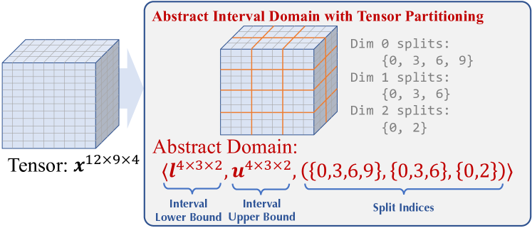
We first formally define our abstraction domain: interval with tensor partitioning. Following the notation in abstract interpretation literature [5], suppose the tensor has $m$ dimensions with shape $n_{1}\times n_{2}\times\cdots\times n_{m}$, we define the abstract domain as such:

$${\mathbb{A}}:=\{\langle{\bm{l}},{\bm{u}},(S_{i})_{i=1}^{m}\rangle:{\bm{l}},{\bm{u}}\in{\mathbb{R}}^{n^{\prime}_{1}\times\cdots\times n^{\prime}_{m}}$$ (6)

$$\hskip 50.00008pt|S_{i}|=n^{\prime}_{i},\forall s\in S_{i},s\in{\mathbb{N}},0\leq s<n_{i}\}.$$

Each element in ${\mathbb{A}}$ is a triplet $a=\langle{\bm{l}},{\bm{u}},(S_{i})_{i=1}^{m}\rangle$, where the first two elements are subblock-wise interval lower bound and upper bound, respectively, and the last element $(S_{1},S_{2},\dots,S_{m})$ contains $m$ sets, where each set $S_{i}$ corresponds to the 0-indexed split indices for the $i$-th dimension to form subblocks. We use $S_{i}[j]\in{\mathbb{N}}$ to represent the $j$-th element of split index set $S_{i}$ sorted in ascending order and define $S_{i}[|S_{i}|]=n_{i}$. Figure 5 illustrates this abstraction domain.

To define the correspondence between the abstract domain and concrete domain ${\mathbb{C}}:=2^{{\mathbb{R}}^{n_{1}\times\cdots\times n_{m}}}$, we form Galois connection $\langle{\mathbb{C}},\subseteq\rangle\underset{\gamma}{\overset{\alpha}{\rightleftharpoons}}\langle{\mathbb{A}},\sqsubseteq\rangle$, where an abstraction function $\alpha:{\mathbb{C}}\to{\mathbb{A}}$ and the concretization function $\gamma:{\mathbb{A}}\to{\mathbb{C}}$ are defined as follows:

$$\alpha({\mathcal{X}})=\langle{\bm{l}},{\bm{u}},(S_{i})_{i=1}^{m}\rangle\quad\text{where}$$ (7a)

$$\hskip 18.00003pt{\bm{l}}_{i_{1},i_{2},\dots,i_{m}}=\min_{{\bm{x}}\in{\mathcal{X}}}\min_{\begin{subarray}{c}1\leq k\leq m\\ S_{k}[i_{k}]\leq j_{k}<S_{k}[i_{k}+1]\end{subarray}}{\bm{x}}_{j_{1},j_{2},\dots,j_{m}},$$

$$\hskip 18.00003pt{\bm{u}}_{i_{1},i_{2},\dots,i_{m}}=\max_{{\bm{x}}\in{\mathcal{X}}}\max_{\begin{subarray}{c}1\leq k\leq m\\ S_{k}[i_{k}]\leq j_{k}<S_{k}[i_{k}+1]\end{subarray}}{\bm{x}}_{j_{1},j_{2},\dots,j_{m}},$$

$$\gamma(\langle{\bm{l}},{\bm{u}},(S_{i})_{i=1}^{m}\rangle)=\{{\bm{x}}: {\bm{l}}_{i_{1},i_{2},\cdots,i_{m}}\leq{\bm{x}}_{j_{1},j_{2},\cdots,j_{m}}\leq{\bm{u}}_{i_{1},i_{2},\cdots,i_{m}},$$ (7b)

$$S_{k}[i_{k}]\leq j_{k}<S_{k}[i_{k}+1],1\leq k\leq m\}.$$

In Equation 7a, the split indices $(S_{i})_{i=1}^{m}$ can be arbitrarily chosen but need to be kept consistent with those in Equation 7b. Take Figure 5 as the example, to abstract a set of tensors ${\mathcal{X}}$ with shape $12\times 9\times 4$, we define split indices for each dimension, respectively, then impose interval constraints on each subblock of the tensor. For example, $[{\bm{l}}_{0,0,0},{\bm{u}}_{0,0,0}]$ constrain any element in ${\bm{x}}_{0:2,0:2,0:1}$, $[{\bm{l}}_{3,2,1},{\bm{u}}_{3,2,1}]$ constrain any element in ${\bm{x}}_{9:11,6:8,2:3}$.

Abstraction Characteristics. There are multiple ways to compute the abstractions, and we design our particular computational algorithms to achieve soundness, tightness, and differentiability. (1) Soundness: We guarantee that all abstractions are sound. Formally, suppose $a_{\bm{x}}$ and $a_{\bm{w}}$ are the abstractions for input and weights, respectively, we guarantee $f_{n}^{*}(\gamma(a_{\bm{x}});\gamma(a_{\bm{w}}))\subseteq\gamma(T_{n}^{*}(a_{\bm{x}};a_{\bm{w}}))$ where $*\in\{\mathsf{in},\mathsf{out}\}$, $n$ is any node in the architecture, and $T_{n}^{*}(a_{\bm{x}};a_{\bm{w}})$ is our computed abstract domain for input or output of node $n$. The soundness property theoretically guarantees that our detection approach has no false negatives, i.e., flag all potential numerical defects, and the validity of generated preconditions (see Section II-B).
(2) Tightness: For most operators in DNN, given abstractions for its inputs, we compute the tightest possible interval abstraction for the output. Formally, for any atomic DNN operator $op$ and any abstract domain $i\in{\mathbb{A}}$ of $op$’s input, if $op(\gamma(i))\subseteq[{\bm{l}},{\bm{u}}]$, i.e., $[{\bm{l}},{\bm{u}}]$ is an interval abstraction of $op$’s output, then $\gamma(T_{op}(i))\subseteq[{\bm{l}},{\bm{u}}]$, i.e., our generated abstract domain $T_{op}(i)$ is always tighter or equal to any interval abstraction $[{\bm{l}},{\bm{u}}]$. Such tightness can reduce false positives for detecting potential numerical defects and increase the span of generated failure-exhibiting intervals and fix intervals, which improves the quality of generated tests and preconditions.
(3) Differentiability: We compute differentiable abstractions. Concretely, if the input of node $n_{2}$ is deferentially dependent on output of node $n_{1}$, we can compute out gradients $\nabla_{i}o$ for any $i\in\{{\bm{l}}_{n_{1}},{\bm{u}}_{n_{1}}\}$ and any $o\in\{{\bm{l}}_{n_{2}},{\bm{u}}_{n_{2}}\}$, where $\langle{\bm{l}}_{n_{1}},{\bm{u}}_{n_{1}},(S^{n_{1}}_{i})_{i=1}^{\dim(n_{1}.\mathsf{out})}\rangle$ and $\langle{\bm{l}}_{n_{2}},{\bm{u}}_{n_{2}},(S^{n_{2}}_{i})_{i=1}^{\dim(n_{2}.\mathsf{in})}\rangle$ are abstractions of $f^{\mathsf{out}}_{n_{1}}(\cdot;\cdot)$ and $f^{\mathsf{in}}_{n_{2}}(\cdot;\cdot)$, respectively. When tightness and differentiability cannot be achieved at the same time (e.g., for floor operator, tight abstraction $\langle{\bm{l}},{\bm{u}}\rangle\mapsto\langle\lfloor{\bm{l}}\rfloor,\lfloor{\bm{u}}\rfloor\rangle$ is not generally differentiable, and differentiable abstraction $\langle{\bm{l}},{\bm{u}}\rangle\mapsto\langle{\bm{l}}-\mathbf{1},{\bm{u}}\rangle$ is not tight), we implement two abstract algorithms to achieve tightness and differentiability, respectively.

The existing approach DEBAR [61] also proposes a static analysis framework for DNN architectures with tensor partitioning. In contrast to our framework, the abstract domain in DEBAR contains affine equalities besides interval domains. Therefore, DEBAR can be tighter than ours in some cases and can produce fewer positives, but due to the additional complexity of affine equalities, DEBAR tends to use the coarsest abstraction (i.e., tensor partitioning) granularity and supports fewer operators than ours. At the same time, our algorithms produce the tightest interval abstractions while DEBAR has no tightness guarantee. As a result, RANUM detects more true numerical defects and has a comparable number of false positives (see Section IV-A), and we can leverage the feasibility confirmation support in RANUM to filter out false positives.

-C2 Initial Abstraction Construction with Backward Fine-Grained Node Labeling

We construct abstract domains for initial nodes in two steps: First, we determine the tensor partitions, i.e., the split index sets $(S_{i})_{i=1}^{m}$ (see Equation 6), which determine the tightness and efficiency of our static analysis framework, because the tensor partitions of all other nodes will be solely dependent on the partitions of initial nodes as we will show in Section -C3. Second, we compute the interval bounds ${\bm{l}}$ and ${\bm{u}}$.

We use the following principle to decide the tensor partitions: For nodes that are connected to operators requiring fine-grained abstractions (e.g., the shape input for operator Reshape) with valid paths (which we will specify later), we construct tensor partitions with the finest granularity, i.e., $S_{i}=\{0,1,\dots,n_{i}\}$. We call these nodes fine-grained initial nodes and starting from the next paragraph we introduce our novel technique of backward fine-grained node labeling to find them out. For other nodes, we rely on downstream task requirements and user specifications to determine the partitions. For example, for fix generation (see Section III-C), we use the coarsest granularity by default.

Backward Fine-Grained Node Labeling. The fine-grained initial nodes are those starting a valid path in DNN computational graph ${\mathcal{G}}$, where a path is valid if and only if the path does not traverse through fine-grained stopping operators and terminates at a fine-grained requiring operator with some specific input indices. As discussed in Section III-A, the fine-grained requiring operators fall into three categories: control-flow operators (e.g., Loop), indexing operators (e.g., Slice), and shaping operators (e.g., Reshape). Fine-grained stopping operators are those whose output is independent of input abstraction granularity (so the granularity of preceding nodes does not matter). Detail lists of fine-grained stopping operators and fine-grained requiring operators are provided in Section -C4.

To find out fine-grained initial nodes, we propose backward fine-grained node labeling, which is similar to data dependency analysis in traditional programs: First, we invert all edges of the given computational graph ${\mathcal{G}}=\langle{\mathcal{V}},{\mathcal{E}}\rangle$ to get ${\mathcal{G}}^{\prime}=\langle{\mathcal{V}},{\mathcal{E}}^{\prime}\rangle$. Second, we attach a boolean label for each node $n\in{\mathcal{V}}$ and initialize them with False. Third, we do topology sorting on ${\mathcal{G}}^{\prime}$. When encountering a node $n$ with True, if the node does not contain a fine-grained stopping operator, we propagate this label to all its subsequent nodes; otherwise, we propagate False. When encountering a node $n$ with False, if the node is a fine-grained requiring operator, we propagate True to some subsequent nodes corresponding to specific input indices and False to others; otherwise, propagate False to all subsequent nodes. Lastly, we collect all labels for initial nodes. The nodes with True label are fine-grained initial nodes.

To this point, we have determined the tensor partitions $(S_{i})_{i=1}^{m}$ for all initial nodes, and we now compute ${\bm{l}}$ and ${\bm{u}}$ and thus finish the abstraction domain construction for the valid ranges of initial nodes. Initial nodes are further divided into input, weight, and constant nodes. In practice, most weight nodes and all constant nodes have their initial values stored in the ONNX file, and we directly use Equation 7a with these initial values to compute ${\bm{l}}$ and ${\bm{u}}$. Otherwise, we rely on user specifications and built-in heuristics to determine ${\bm{l}}$ and ${\bm{u}}$ for initial nodes.

-C3 Internal Abstraction with Dynamic Partitioning

For all supported operator types (listed in Section -A), we propose concrete algorithms to compute abstract domains for output with dynamic tensor partitioning. Formally, for each operator $op$, we construct the computable function $T_{op}:{\mathbb{A}}\to{\mathbb{A}}$ that satisfies soundness and tentatively satisfies tightness and differentiability, where ${\mathbb{A}}$ is the abstract domain defined in Equation 6. Therefore, following the computational procedure introduced at the end of Section III-A, we can compute end-to-end abstractions for all nodes in the given DNN architecture. As the showcase of our abstraction algorithm, we describe the algorithms for four representative operators: MatMul, Conv, Softmax, and Loop.

MatMul

The MatMul operator computes the matrix multiplication of two operands. This operator is widely used in DNNs to express fully-connected layers. To simplify the narration, we focus on the two-dimensional case where we compute $op({\bm{A}},{\bm{B}})={\bm{C}}={\bm{A}}{\bm{B}}$ with ${\bm{A}}\in{\mathbb{R}}^{n\times m}$ and ${\bm{B}}\in{\mathbb{R}}^{m\times l}$. Extensions to other dimensions by abstracting the broadcasting mechanism can be found in our open-source implementation.

We denote the input abstractions of $op$ by $a=\langle{\bm{L}}_{a},{\bm{U}}_{a},(S_{A}^{1},S_{A}^{2})\rangle$ and $b=\langle{\bm{L}}_{b},{\bm{U}}_{b},(S_{B}^{1},S_{B}^{2})\rangle$, respectively. First, we compute the union $U=S_{A}^{2}\cup S_{B}^{1}$. Second, we dynamically partition both $a$ and $b$ with split points $(S_{A}^{1},U)$ and $(U,S_{B}^{2})$, respectively, and get $a^{\prime}=\langle{\bm{L}}^{\prime}_{a},{\bm{U}}^{\prime}_{a},(S_{A}^{1},U)\rangle$ and $b^{\prime}=\langle{\bm{L}}^{\prime}_{b},{\bm{U}}^{\prime}_{b},(U,S_{B}^{2})\rangle$. Note that $a$ and $a^{\prime}$ (or $b$ and $b^{\prime}$) correspond to the same concrete domain, but $a^{\prime}$ and $b^{\prime}$ have finer or equal partition granularity than $a$ and $b$. Third, we compute output abstraction $T_{op}(a,b)=c=\langle{\bm{L}}_{c},{\bm{U}}_{c},(S_{A}^{1},S_{B}^{2})\rangle$

$$\text{where}\quad({\bm{L}}_{c})_{ij} =\sum_{k=1}^{|U|}{\bm{v}}_{k}\min_{{\bm{A}}\in\{{\bm{L}}^{\prime}_{a},{\bm{U}}^{\prime}_{a}\},{\bm{B}}\in\{{\bm{L}}^{\prime}_{b},{\bm{U}}^{\prime}_{b}\}}{\bm{A}}_{ik}{\bm{B}}_{kj},$$ (8)

$$({\bm{U}}_{c})_{ij} =\sum_{k=1}^{|U|}{\bm{v}}_{k}\max_{{\bm{A}}\in\{{\bm{L}}^{\prime}_{a},{\bm{U}}^{\prime}_{a}\},{\bm{B}}\in\{{\bm{L}}^{\prime}_{b},{\bm{U}}^{\prime}_{b}\}}{\bm{A}}_{ik}{\bm{B}}_{kj},$$

$${\bm{v}}_{k} =U[k]-U[k-1].$$

This formulation can guarantee tightness but is not efficient for tensor computation due to the inner minimum and maximum. Therefore, we also implement a fast-mode abstraction trading tightness for efficiency: $T_{op}^{\prime}(a,b)=c^{\prime}=\langle{\bm{L}}_{c}^{\prime},{\bm{U}}_{c}^{\prime},(S_{A}^{1},S_{B}^{2})\rangle$ where

$${\bm{L}}_{c}^{{}^{\prime}}= {\bm{U}}_{a}^{{}^{\prime}-}{\bm{v}}{\bm{U}}_{b}^{{}^{\prime}-}+{\bm{U}}_{a}^{{}^{\prime}0}{\bm{v}}{\bm{L}}_{b}^{{}^{\prime}-}+{\bm{U}}_{a}^{{}^{\prime}+}{\bm{v}}{\bm{L}}_{b}^{{}^{\prime}-}+$$ (9)

$${\bm{L}}_{a}^{{}^{\prime}-}{\bm{v}}{\bm{U}}_{b}^{{}^{\prime}0}+{\bm{U}}_{a}^{{}^{\prime}0}{\bm{v}}{\bm{L}}_{b}^{{}^{\prime}0}+{\bm{L}}_{a}^{{}^{\prime}0}{\bm{v}}{\bm{U}}_{b}^{{}^{\prime}0}+{\bm{U}}_{a}^{{}^{\prime}+}{\bm{v}}{\bm{L}}_{b}^{{}^{\prime}0}+$$

$${\bm{L}}_{a}^{{}^{\prime}-}{\bm{v}}{\bm{U}}_{b}^{{}^{\prime}+}+{\bm{L}}_{a}^{{}^{\prime}0}{\bm{v}}{\bm{U}}_{b}^{{}^{\prime}+}+{\bm{L}}_{a}^{{}^{\prime}+}{\bm{v}}{\bm{L}}_{b}^{{}^{\prime}+},$$

$${\bm{U}}_{c}^{{}^{\prime}}= {\bm{L}}_{a}^{{}^{\prime}-}{\bm{v}}{\bm{L}}_{b}^{{}^{\prime}-}+{\bm{L}}_{a}^{{}^{\prime}0}{\bm{v}}{\bm{L}}_{b}^{{}^{\prime}-}+{\bm{L}}_{a}^{{}^{\prime}+}{\bm{v}}{\bm{U}}_{b}^{{}^{\prime}-}+$$

$${\bm{L}}_{a}^{{}^{\prime}-}{\bm{v}}{\bm{L}}_{b}^{{}^{\prime}0}+{\bm{L}}_{a}^{{}^{\prime}0}{\bm{v}}{\bm{L}}_{b}^{{}^{\prime}0}+{\bm{U}}_{a}^{{}^{\prime}0}{\bm{v}}{\bm{U}}_{b}^{{}^{\prime}0}+{\bm{U}}_{a}^{{}^{\prime}+}{\bm{v}}{\bm{U}}_{b}^{{}^{\prime}0}+$$

$${\bm{U}}_{a}^{{}^{\prime}-}{\bm{v}}{\bm{L}}_{b}^{{}^{\prime}+}+{\bm{U}}_{a}^{{}^{\prime}0}{\bm{v}}{\bm{U}}_{b}^{{}^{\prime}+}+{\bm{U}}_{a}^{{}^{\prime}+}{\bm{v}}{\bm{U}}_{b}^{{}^{\prime}+}.$$

In the above equation, for any $*\in\{a,b\}$, let $\circ$ be the elementwise (Hadamard) product,

$${\bm{L}}_{*}^{{}^{\prime}-}= {\bm{L}}_{*}^{{}^{\prime}}\circ{\mathbb{I}}[{\bm{U}}_{*}^{{}^{\prime}}<0],{\bm{U}}_{*}^{{}^{\prime}-}={\bm{U}}_{*}^{{}^{\prime}}\circ{\mathbb{I}}[{\bm{U}}_{*}^{{}^{\prime}}<0],$$ (10)

$${\bm{L}}_{*}^{{}^{\prime}0}= {\bm{L}}_{*}^{{}^{\prime}}\circ{\mathbb{I}}[{\bm{L}}_{*}^{{}^{\prime}}\leq 0,{\bm{U}}_{*}^{{}^{\prime}}\geq 0],{\bm{U}}_{*}^{{}^{\prime}0}={\bm{U}}_{*}^{{}^{\prime}}\circ{\mathbb{I}}[{\bm{L}}_{*}^{{}^{\prime}}\leq 0,{\bm{U}}_{*}^{{}^{\prime}}\geq 0],$$

$${\bm{L}}_{*}^{{}^{\prime}+}= {\bm{L}}_{*}^{{}^{\prime}}\circ{\mathbb{I}}[{\bm{L}}_{*}^{{}^{\prime}}>0],{\bm{U}}_{*}^{{}^{\prime}+}={\bm{U}}_{*}^{{}^{\prime}}\circ{\mathbb{I}}[{\bm{L}}_{*}^{{}^{\prime}}>0].$$

From Equation 9, we can observe that the abstraction can be easily implemented with tensor computations. In Section -C5, we prove the soundness and tightness of these abstractions.

Conv

The Conv operator computes the discrete convolution of two operands. This operator is widely used in convolutional neural networks (CNNs, [15]). To simplify the narration, we focus on the single-channel single-stride two-dimensional case where we compute $op({\bm{A}},{\bm{W}})={\bm{C}}$ with ${\bm{A}}$ being the input matrix and ${\bm{W}}$ being the convolution kernel. Extensions to general cases are provided in our open-source implementation.

We first dynamically split the kernel abstraction to the finest granularity. Second, we compute the receptive field, which is the sub-region of ${\bm{A}}$ that decides each output position, of each output position. Third, we inspect the alignment between receptive fields and ${\bm{A}}$’s partitions. If neighboring output positions have their receptive fields partitioned in the same sub-block of ${\bm{A}}$, it means that these positions can be abstracted by a single interval, i.e., these positions can be partitioned together. Fourth, using this principle, we derive the partitions of the output tensor, and repeat the input tensors accordingly and efficiently so that the abstract computation can be written as convolutional operations. Last, we modify the abstraction computation equations in Equation 9 by replacing matrix multiplication with convolution to compute the abstraction of output ${\bm{C}}$.

Softmax

The Softmax operator computes normalized exponential values for the given input. Softmax is widely deployed for classification tasks to yield normalized confidence. In one-dimensional case, for input ${\bm{x}}\in{\mathbb{R}}^{n}$, a Softmax operator outputs $op({\bm{x}})=\frac{\exp({\bm{x}})}{\sum_{i=1}^{n}\exp({\bm{x}})_{i}}$. The output abstraction of Softmax operator $op$ can be thus computed: $T_{op}(\langle{\bm{l}},{\bm{u}},(S)\rangle)=\langle{\bm{l}}^{o},{\bm{u}}^{o},(S)\rangle$ where

The output abstraction’s partition is dynamically decided by the input abstraction’s partition. We prove the soundness and tightness of the abstraction in Section -C5.

Loop

The node with a Loop operator contains a sub-computational graph with dynamic controlling counters and conditions to represent a runtime loop. The Loop operator can be used to represent recurrent neural networks (RNNs) and handle the input sequence of variable length. We require the controlling counter and loop termination condition to have the finest abstraction granularity. Then, we recursively apply our static analysis framework to the sub-graph representing the loop body and update the interval of the loop counter iteratively. When the abstraction interval of the loop counter can explicitly decide whether to terminate the loop, we continue or terminate the loop iterations, respectively; otherwise, we merge the current abstraction interval with the interval obtained after another iteration. We repeat this process until termination. Theoretically, this execution process cannot guarantee the termination, i.e., the loop body may execute for infinite times. However, in practice, on our dataset, our analysis framework already suffices to guarantee the termination in all cases. In the future, we can apply a widening operation if termination cannot be tightly abstracted.

Remark.

As we can see, the novel dynamic partition technique is incorporated into the computation process of each operator’s abstraction. The soundness and tightness of our designed abstractions are immediately achieved by design, and the differentiability of our designed abstractions can be implemented via the auto-differentiation functionality of popular DL libraries like PyTorch [28] and Tensorflow [1] where we use PyTorch for implementation. The abstractions for DNNs are also implemented for other applications, e.g., for robustness verification [40, 25]. However, our abstractions are tailored for the tensor-partitioned interval domain that is particularly suitable for testing and debugging the numerical defects. To the best of our knowledge, these abstractions are the first that achieve soundness, tightness, and differentiability.

-C4 List of Fine-Grained Requiring and Stopping Operators

We use fine-grained requiring and fine-grained stopping operators in Section -C2. Among all supported operators, the fine-grained requiring operators are

Reshape (input #2), Slice (input #2, #3, #4, #5), Squeeze (input #2), Unsqueeze (input #2), Tile (input #2, #3), Loop (input #1, #2), SequenceInsert (input #3), ConstantOfShape (input #1), Gather (input #2), GatherND (input #2), ReduceSum (input #2), ScatterElements (input #2), Expand (input #2), Split (input #2), Pad (input #2, #3), NegativeLogLikelihoodLoss (input #2), Clip (input #2, #3), OneHot (input #2), Resize (input #2, #3, #4).

The fine-grained stopping operators are

Shape, RandomNormalLike, RandomUniformLike.

-C5 Proofs

Here we present the omitted proofs in Section -C3.

MatMul

Theorem 1 (Tightness of Abstraction by Equation 8 for MatMul).

Suppose $op$ is the MatMul operator and $T_{op}$ is as defined in Equation 8, then if $op(\gamma(a),\gamma(b))\subseteq[{\bm{L}},{\bm{U}}]$ for $a,b\in{\mathbb{A}}$, $\gamma(T_{op}(a,b))\subseteq[{\bm{L}},{\bm{U}}]$.

Proof.

We use ${\bm{L}}_{a}$ and ${\bm{U}}_{a}$ to denote the element-wise interval lower and upper bounds of $\gamma(a)$; and use ${\bm{L}}_{b}$ and ${\bm{U}}_{b}$ to denote these bounds of $\gamma(b)$, respectively, where a formal definition is in Equation 7b. Then, there exist ${\bm{A}}$ and ${\bm{B}}$ with ${\bm{L}}_{a}\leq{\bm{A}}\leq{\bm{U}}_{a}$ and ${\bm{L}}_{b}\leq{\bm{B}}\leq{\bm{U}}_{b}$, such that

$$({\bm{A}}{\bm{B}})_{ij} =\sum_{k=1}^{l}\min\{{\bm{L}}_{a,ik}{\bm{L}}_{b,kj},{\bm{L}}_{a,ik}{\bm{U}}_{b,kj},$$

$$\hskip 45.00008pt{\bm{U}}_{a,ik}{\bm{L}}_{b,kj},{\bm{U}}_{a,ik}{\bm{U}}_{b,kj}\},$$ (12)

$$\text{or }({\bm{A}}{\bm{B}})_{ij} =\sum_{k=1}^{l}\max\{{\bm{L}}_{a,ik}{\bm{L}}_{b,kj},{\bm{L}}_{a,ik}{\bm{U}}_{b,kj},$$

$$\hskip 45.00008pt{\bm{U}}_{a,ik}{\bm{L}}_{b,kj},{\bm{U}}_{a,ik}{\bm{U}}_{b,kj}\}.$$ (13)

By definition, we have

$$\small{\bm{L}}_{ij}\leq\text{\lx@cref{creftypecap~refnum}{eq:pf-1}},{\bm{U}}_{ij}\geq\text{\lx@cref{creftypecap~refnum}{eq:pf-2}}.$$ (14)

We let ${\bm{L}}^{\prime}_{c}$ and ${\bm{U}}^{\prime}_{c}$ to denote the element-wise interval lower and upper bounds for $\gamma(T_{op}(a,b))$, let $S_{A}^{1}[i^{\prime}]\leq i-1<S_{A}^{1}[i^{\prime}+1]$ and $S_{B}^{2}[j^{\prime}]\leq j-1<S_{B}^{2}[j^{\prime}+1]$, then from Equation 8,

$$({\bm{L}}^{\prime}_{c})_{ij}=({\bm{L}}_{c})_{i^{\prime}j^{\prime}}$$ (15)

$$= \sum_{k=1}^{|U|}\sum_{k^{\prime}=U[k-1]+1}^{U[k]}\min\{{\bm{L}}_{a,ik^{\prime}}{\bm{L}}_{b,k^{\prime}j},{\bm{L}}_{a,ik^{\prime}}{\bm{U}}_{b,k^{\prime}j},$$

$$\hskip 90.00015pt{\bm{U}}_{a,ik^{\prime}}{\bm{L}}_{b,k^{\prime}j},{\bm{U}}_{a,ik^{\prime}}{\bm{U}}_{b,k^{\prime}j}\}$$

$$= \sum_{k=1}^{l}\min\{{\bm{L}}_{a,ik}{\bm{L}}_{b,kj},{\bm{L}}_{a,ik}{\bm{U}}_{b,kj},{\bm{U}}_{a,ik}{\bm{L}}_{b,kj},{\bm{U}}_{a,ik}{\bm{U}}_{b,kj}\}$$

$$= \text{\lx@cref{creftypecap~refnum}{eq:pf-1}}\geq{\bm{L}}_{ij}.$$

Similarly, $({\bm{U}}^{\prime}_{c})_{ij}\leq{\bm{U}}_{ij}$. Thus, $\gamma(T_{op}(a,b))\subseteq[{\bm{L}},{\bm{U}}]$. ∎

Theorem 2 (Soundness of Abstraction by Equation 8 for MatMul).

Suppose $op$ is the MatMul opeartor and $T_{op}$ is as defined in Equation 8, then $op(\gamma(a),\gamma(b))\subseteq\gamma(T_{op}(a,b))$.

Proof.

We use ${\bm{L}}_{a}$ and ${\bm{U}}_{a}$ to denote the element-wise interval lower and upper bounds of $\gamma(a)$; and use ${\bm{L}}_{b}$ and ${\bm{U}}_{b}$ to denote these bounds of $\gamma(b)$, respectively, where a formal definition is in Equation 7b. For any ${\bm{A}}$ and ${\bm{B}}$ such that ${\bm{L}}_{a}\leq{\bm{A}}\leq{\bm{U}}_{a}$ and ${\bm{L}}_{b}\leq{\bm{B}}\leq{\bm{U}}_{b}$,

$$({\bm{A}}{\bm{B}})_{ij} =\sum_{k=1}^{l}{\bm{A}}_{ik}{\bm{B}}_{kj}$$ (16)

$$\geq\min\{{\bm{L}}_{a,ik}{\bm{L}}_{b,kj},{\bm{L}}_{a,ik}{\bm{U}}_{b,kj},{\bm{U}}_{a,ik}{\bm{L}}_{b,kj},{\bm{U}}_{a,ik}{\bm{U}}_{b,kj}\}$$

$$=:({\bm{L}}_{ab}^{\prime})_{ij}$$

and

$$({\bm{A}}{\bm{B}})_{ij} \leq\max\{{\bm{L}}_{a,ik}{\bm{L}}_{b,kj},{\bm{L}}_{a,ik}{\bm{U}}_{b,kj},{\bm{U}}_{a,ik}{\bm{L}}_{b,kj},{\bm{U}}_{a,ik}{\bm{U}}_{b,kj}\}$$ (17)

$$=:({\bm{U}}_{ab}^{\prime})_{ij}.$$

Thus, $op(\gamma(a),\gamma(b))\subseteq[{\bm{L}}^{\prime}_{ab},{\bm{U}}^{\prime}_{ab}]$. On the other hand, $\gamma(T_{op}(a,b))=[{\bm{L}}^{\prime}_{ab},{\bm{U}}^{\prime}_{ab}]$ as seen from Equation 15. Therefore, $op(\gamma(a),\gamma(b))\subseteq\gamma(T_{op}(a,b))$. ∎

Theorem 3 (Soundness of Abstraction by Equation 9 for MatMul).

Suppose $op$ is the MatMul operator and $T^{\prime}_{op}$ is as defined in Equations 9 and 10, then $op(\gamma(a),\gamma(b))\subseteq\gamma(T^{\prime}_{op}(a,b))$.

Proof.

We use ${\bm{L}}_{a}$ and ${\bm{U}}_{a}$ to denote the element-wise interval lower and upper bounds of $\gamma(a)$; and use ${\bm{L}}_{b}$ and ${\bm{U}}_{b}$ to denote these bounds of $\gamma(b)$, respectively, where a formal definition is in Equation 7b. We define ${\bm{L}}^{\prime}_{ab}$ and ${\bm{U}}^{\prime}_{ab}$ by Equations 16 and 17. From the proof of Theorem 2, we have $op(\gamma(a),\gamma(b))\subseteq[{\bm{L}}^{\prime}_{ab},{\bm{U}}^{\prime}_{ab}]$. We now only need to show that $[{\bm{L}}^{\prime}_{ab},{\bm{U}}^{\prime}_{ab}]\subseteq\gamma(T^{\prime}_{op}(a,b))$.

$\gamma(T^{\prime}_{op}(a,b))$ imposes independent interval abstractions element-wise, therefore, we study each element independently. For the element $(i,j)$, from Equations 9 and 10, the interval lower bound of $\gamma(T^{\prime}_{op}(a,b))$, namely $({\bm{L}}_{c})_{ij}$, satisfies

$$({\bm{L}}_{c})_{ij}=\sum_{k=1}^{l}({\bm{U}}_{a}^{-})_{ik}({\bm{U}}_{b}^{-})_{kj}+({\bm{U}}_{a}^{0})_{ik}({\bm{L}}_{b}^{-})_{kj}+({\bm{U}}_{a}^{+})_{ik}({\bm{L}}_{b}^{-})_{kj}+$$ (18)

$$({\bm{L}}_{a}^{-})_{ik}({\bm{U}}_{b}^{0})_{kj}+({\bm{U}}_{a}^{0})_{ik}({\bm{L}}_{b}^{0})_{kj}+({\bm{L}}_{a}^{0})_{ik}({\bm{U}}_{b}^{0})_{kj}+({\bm{U}}_{a}^{+})_{ik}({\bm{L}}_{b}^{0})_{kj}+$$

$$({\bm{L}}_{a}^{-})_{ik}({\bm{U}}_{b}^{+})_{kj}+({\bm{L}}_{a}^{0})_{ik}({\bm{U}}_{b}^{+})_{kj}+({\bm{L}}_{a}^{+})_{ik}({\bm{L}}_{b}^{+})_{kj}.$$

By Equation 10,

• when ${\bm{L}}_{a,ik}\leq{\bm{U}}_{a,ik}<0$,
  $({\bm{L}}_{a}^{-})_{ik}={\bm{L}}_{a,ik},({\bm{U}}_{a}^{-})_{ik}={\bm{U}}_{a,ik},({\bm{L}}_{a}^{0})_{ik}=0,\\ ({\bm{U}}_{a}^{0})_{ik}=0,({\bm{L}}_{a}^{+})_{ik}=0,({\bm{U}}_{a}^{+})_{ik}=0$;

• when ${\bm{L}}_{a,ik}\leq 0\leq{\bm{U}}_{a,ik}$,
  $({\bm{L}}_{a}^{-})_{ik}=0,({\bm{U}}_{a}^{-})_{ik}=0,({\bm{L}}_{a}^{0})_{ik}={\bm{L}}_{a,ik},\\ ({\bm{U}}_{a}^{0})_{ik}={\bm{U}}_{a,ik},({\bm{L}}_{a}^{+})_{ik}=0,({\bm{U}}_{a}^{+})_{ik}=0$;

• when $0<{\bm{L}}_{a,ik}\leq{\bm{U}}_{a,ik}$,
  $({\bm{L}}_{a}^{-})_{ik}=0,({\bm{U}}_{a}^{-})_{ik}=0,({\bm{L}}_{a}^{0})_{ik}=0,\\ ({\bm{U}}_{a}^{0})_{ik}=0,({\bm{L}}_{a}^{+})_{ik}={\bm{L}}_{a,ik},({\bm{U}}_{a}^{+})_{ik}={\bm{U}}_{a,ik}$.

Similarly for $({\bm{L}}_{b}^{-})_{kj}$, $({\bm{U}}_{b}^{-})_{kj}$, $({\bm{L}}_{b}^{0})_{kj}$, $({\bm{U}}_{b}^{0})_{kj}$, $({\bm{L}}_{b}^{+})_{kj}$ and $({\bm{U}}_{b}^{+})_{kj}$. Thus, by enumerating all cases, we have

$$\text{\lx@cref{creftypecap~refnum}{eq:pf-6}}\leq\min\{ {\bm{L}}_{a,ik}{\bm{L}}_{b,kj},{\bm{L}}_{a,ik}{\bm{U}}_{b,kj},$$ (19)

$${\bm{U}}_{a,ik}{\bm{L}}_{b,kj},{\bm{U}}_{a,ik}{\bm{U}}_{b,kj}\}=({\bm{L}}^{\prime}_{ab})_{ij}.$$

Similarly, the interval lower bound of $\gamma(T^{\prime}_{op}(a,b))$, namely $({\bm{U}}_{c})_{ij}$,

$$({\bm{U}}_{c})_{ij}\geq\max\{ {\bm{L}}_{a,ik}{\bm{L}}_{b,kj},{\bm{L}}_{a,ik}{\bm{U}}_{b,kj},$$ (20)

$${\bm{U}}_{a,ik}{\bm{L}}_{b,kj},{\bm{U}}_{a,ik}{\bm{U}}_{b,kj}\}=({\bm{U}}^{\prime}_{ab})_{ij}.$$

Thus, $[{\bm{L}}^{\prime}_{ab},{\bm{U}}^{\prime}_{ab}]\subseteq\gamma(T^{\prime}_{op}(a,b))$. ∎

Softmax

Theorem 4 (Tightness of Abstraction for Softmax).

Suppose $op:{\mathbb{R}}^{n}\to{\mathbb{R}}^{n}$ is the Softmax operator and $T_{op}$ is as defined in Equation 11, if $op(\gamma(\langle{\bm{l}},{\bm{u}},(S)\rangle))\subseteq[{\bm{l}}^{r},{\bm{u}}^{r}]$, then $\gamma(T_{op}(\langle{\bm{l}},{\bm{u}},(S)\rangle))\subseteq[{\bm{l}}^{r},{\bm{u}}^{r}]$.

Proof.

We use ${\bm{l}}^{\prime}$ and ${\bm{u}}^{\prime}$ to denote the element-wise interval lower and upper bounds of $\gamma(\langle{\bm{l}},{\bm{u}},(S)\rangle)$. Formally, ${\bm{l}}^{\prime}_{i}={\bm{l}}_{i^{\prime}}$ and ${\bm{u}}^{\prime}_{i}={\bm{u}}_{i^{\prime}}$ where $S[i^{\prime}]\leq i-1<S[i^{\prime}+1]$. Then, for each $i$, by setting ${\bm{x}}_{i}={\bm{l}}_{i}$ and ${\bm{x}}_{j}={\bm{u}}_{j}$ for all $j\neq i$, we get

$${\bm{l}}_{i}^{r} \leq\dfrac{\exp({\bm{l}}^{\prime}_{i})}{\exp({\bm{l}}^{\prime}_{i})+\sum_{k=1,k\neq i}^{n}\exp({\bm{u}}^{\prime}_{k})}$$ (21)

$$=\dfrac{\exp({\bm{l}}_{i^{\prime}})}{\exp({\bm{l}}_{i^{\prime}})+\sum_{k=1}^{n}\exp({\bm{u}}^{\prime}_{k})-\exp({\bm{u}}^{\prime}_{i})}$$

$$=\dfrac{\exp({\bm{l}}_{i^{\prime}})}{\exp({\bm{l}}_{i^{\prime}})+{\bm{v}}^{\scriptscriptstyle\mathsf{T}}\exp({\bm{u}}_{k})-\exp({\bm{u}}_{i^{\prime}})}={\bm{l}}_{i^{\prime}}^{o}.$$

In addition, by setting ${\bm{x}}_{i}={\bm{u}}_{i}$ and ${\bm{x}}_{j}={\bm{l}}_{j}$ for all $j\neq i$, we get ${\bm{u}}_{i}^{r}\geq{\bm{u}}_{i^{\prime}}^{o}$. Here, ${\bm{l}}^{o}$ and ${\bm{u}}^{o}$ are as defined in Equation 11. Combining these two arguments, we get

$$\gamma(T_{op}(\langle{\bm{l}},{\bm{u}},(S)\rangle))\subseteq[{\bm{l}}^{r},{\bm{u}}^{r}].$$

∎

Theorem 5 (Soundness of Abstraction for Softmax).

Suppose $op:{\mathbb{R}}^{n}\to{\mathbb{R}}^{n}$ is the Softmax operator and $T_{op}$ is as defined in Equation 11, then $op(\gamma(\langle{\bm{l}},{\bm{u}},(S)\rangle))\subseteq\gamma(T_{op}(\langle{\bm{l}},{\bm{u}},(S)\rangle))$.

Proof.

Leveraging the fact that the softmax function is monotonically increasing, i.e., $\frac{\mathrm{d}op({\bm{x}})_{i}}{\mathrm{d}{\bm{x}}_{j}}>0$, we have $\gamma(\langle{\bm{l}},{\bm{u}},(S)\rangle)_{i}\in[{\bm{l}}^{o}_{i^{\prime}},{\bm{u}}^{o}_{i^{\prime}}]$, where $S[i^{\prime}]\leq i-1<S[i^{\prime}+1]$. Since $[{\bm{l}}^{o}_{i^{\prime}},{\bm{u}}^{o}_{i^{\prime}}]=\gamma(T_{op}(\langle{\bm{l}},{\bm{u}},(S)\rangle))_{i}$ by our definition of $T_{op}$, $op(\gamma(\langle{\bm{l}},{\bm{u}},(S)\rangle))\subseteq\gamma(T_{op}(\langle{\bm{l}},{\bm{u}},(S)\rangle))$ follows. ∎

-D Implementation

We have implemented a tool for RANUM in roughly 10k lines of Python code based on PyTorch. Our tool leverages existing modules (tf2onnx for PyTorch and torch.onnx.export for Tensorflow and Keras) to extract ONNX-format DNN architectures from DL programs to take as the input, and automatically generates detection results, system tests, and defect fixes (given imposing locations).

-E Hyperparameters

In this section, we listed hyperparameters in our two-step system test generation technique: For the unit test generation, we use the Adam optimizer where the learning rate is $1$ and the maximum iteration number is $100$. For the training example generation, we target for training example under learning rate $\gamma=1$ and the approach has similar performance under other learning rates. We follow the convention in the DLG attack, where we use the L-BFGS method as the optimizer for gradient-based minimization. We terminate the method and return “failed” if either the running time exceeds $1800\text{\,}\mathrm{s}$ (universal execution time limit for all experimental evaluations), or a failure-exhibiting example training is not found after $300$ iterations of L-BFGS optimization.

-F Ablation Study of System Test Generation

RANUM uses the two-step test generation technique to produce failure-exhibiting system tests: it first generates failure-exhibiting unit tests with gradient back-propagation, then generates failure-exhibiting training examples via the extended DLG attack. To isolate the impact of RANUM at each step, we replace either step with random sampling: “Random + RANUM”, which first generates failure-exhibiting unit tests via random sampling, then generates training example via RANUM; “RANUM + Random”, which first generates failure-exhibiting unit tests via RANUM, then generates training example via random sampling. We follow the same evaluation protocol as in Section IV-B in this ablation study. We find that “RANUM + Random” takes 9.38X running time than RANUM and fails for 68 runs (RANUM only fails for 57 runs); and “Random + RANUM” fails for 113 runs (roughly 2X failed runs compared to RANUM). This study implies that RANUM’s technique helps to improve effectiveness and efficiency at both steps of failure-exhibiting system test generation compared to the pure random baseline. The improvement for the first step is mainly from the effectiveness perspective, and the improvement for the second step is mainly from the efficiency perspective.

-G Threats to Validity

An external threat to validity is the evaluation subjects, which are the GRIST benchmarks [54], used to evaluate RANUM and baseline approaches. Although the subjects contain 63 real-world DL programs and are the largest to our knowledge, they still may not be representative enough. Another external threat is the approach randomness. To mitigate this threat, we repeat all randomized approaches for 10 runs. To mitigate bias in the empirical study, two authors independently conduct the study and discuss all cases to reach a consensus. A major internal threat to validity comes from the approach implementation. We reduce this threat by conducting code review and log checking extensively. An author independently checks the correctness of code implementation. We also verify the soundness of our static analysis framework with over 50 carefully designed unit tests.

References

- Abadi et al. [2016] M. Abadi, A. Agarwal, P. Barham, E. Brevdo, Z. Chen, C. Citro, G. S. Corrado, A. Davis, J. Dean, M. Devin, S. Ghemawat, I. J. Goodfellow, A. Harp, G. Irving, M. Isard, Y. Jia, R. Józefowicz, L. Kaiser, M. Kudlur, J. Levenberg, D. Mané, R. Monga, S. Moore, D. G. Murray, C. Olah, M. Schuster, J. Shlens, B. Steiner, I. Sutskever, K. Talwar, P. A. Tucker, V. Vanhoucke, V. Vasudevan, F. B. Viégas, O. Vinyals, P. Warden, M. Wattenberg, M. Wicke, Y. Yu, and X. Zheng, “TensorFlow: Large-scale machine learning on heterogeneous distributed systems,” CoRR, vol. abs/1603.04467, 2016.
- Albarghouthi [2021] A. Albarghouthi, “Introduction to neural network verification,” Foundations and Trends in Programming Languages, vol. 7, no. 1-2, pp. 1–157, 2021.
- Bengio et al. [2013] Y. Bengio, N. Léonard, and A. C. Courville, “Estimating or propagating gradients through stochastic neurons for conditional computation,” CoRR, vol. abs/1308.3432, 2013.
- Bui et al. [2021] N. D. Q. Bui, Y. Yu, and L. Jiang, “InferCode: Self-supervised learning of code representations by predicting subtrees,” in 43rd IEEE/ACM International Conference on Software Engineering, ICSE. IEEE, 2021, pp. 1186–1197.
- Cousot and Cousot [1977] P. Cousot and R. Cousot, “Static determination of dynamic properties of generalized type unions,” in ACM Conference on Language Design for Reliable Software, LDRS. ACM, 1977, pp. 77–94.
- Gehr et al. [2018] T. Gehr, M. Mirman, D. Drachsler-Cohen, P. Tsankov, S. Chaudhuri, and M. Vechev, “AI2: safety and robustness certification of neural networks with abstract interpretation,” in 39th IEEE Symposium on Security and Privacy, SP. IEEE, 2018, pp. 3–18.
- Glorot et al. [2011] X. Glorot, A. Bordes, and Y. Bengio, “Deep sparse rectifier neural networks,” in 14th International Conference on Artificial Intelligence and Statistics, AISTATS. JMLR.org, 2011, pp. 315–323.
- Goodfellow et al. [2015] I. J. Goodfellow, J. Shlens, and C. Szegedy, “Explaining and harnessing adversarial examples,” in 3rd International Conference on Learning Representations, ICLR. OpenReview.net, 2015.
- Guerriero et al. [2021] A. Guerriero, R. Pietrantuono, and S. Russo, “Operation is the hardest teacher: estimating DNN accuracy looking for mispredictions,” in 43rd IEEE/ACM International Conference on Software Engineering, ICSE. IEEE, 2021, pp. 348–358.
- Gurfinkel et al. [2015] A. Gurfinkel, T. Kahsai, A. Komuravelli, and J. A. Navas, “The SeaHorn verification framework,” in 27th International Conference on Computer Aided Verification, CAV. Springer, 2015, pp. 343–361.
- Hattori et al. [2020] M. Hattori, S. Sawada, S. Hamaji, M. Sakai, and S. Shimizu, “Semi-static type, shape, and symbolic shape inference for dynamic computation graphs,” in 4th ACM SIGPLAN International Workshop on Machine Learning and Programming Languages, 2020, pp. 11–19.
- Humbatova et al. [2020] N. Humbatova, G. Jahangirova, G. Bavota, V. Riccio, A. Stocco, and P. Tonella, “Taxonomy of real faults in deep learning systems,” in 42nd ACM/IEEE International Conference on Software Engineering, ICSE. IEEE, 2020, pp. 1110–1121.
- Jay et al. [2019] N. Jay, N. Rotman, B. Godfrey, M. Schapira, and A. Tamar, “A deep reinforcement learning perspective on Internet congestion control,” in 36th International Conference on Machine Learning, ICML. PMLR, 2019, pp. 3050–3059.
- Kloberdanz et al. [2022] E. Kloberdanz, K. G. Kloberdanz, and W. Le, “DeepStability: A study of unstable numerical methods and their solutions in deep learning,” in 44th International Conference on Software Engineering, ICSE. ACM, 2022, pp. 586–597.
- Krizhevsky et al. [2012] A. Krizhevsky, I. Sutskever, and G. E. Hinton, “ImageNet classification with deep convolutional neural networks,” in Advances in Neural Information Processing Systems 25, NIPS, 2012, pp. 1106–1114.
- Li et al. [2019] L. Li, Z. Zhong, B. Li, and T. Xie, “Robustra: Training provable robust neural networks over reference adversarial space,” in 28th International Joint Conference on Artificial Intelligence, IJCAI. ijcai.org, 2019, pp. 4711–4717.
- Li et al. [2023] L. Li, T. Xie, and B. Li, “SoK: Certified robustness for deep neural networks,” in 44th IEEE Symposium on Security and Privacy, SP. IEEE, 2023, pp. 94–115.
- Li and Yuan [2017] Y. Li and Y. Yuan, “Convergence analysis of two-layer neural networks with ReLU activation,” in Advances in Neural Information Processing Systems 30, NIPS, 2017, pp. 597–607.
- Liu et al. [2021] C. Liu, J. Lu, G. Li, T. Yuan, L. Li, F. Tan, J. Yang, L. You, and J. Xue, “Detecting TensorFlow program bugs in real-world industrial environment,” in 36th IEEE/ACM International Conference on Automated Software Engineering, ASE. IEEE, 2021, pp. 55–66.
- Liu et al. [2022] F. Liu, G. Li, B. Wei, X. Xia, Z. Fu, and Z. Jin, “A unified multi-task learning model for AST-level and token-level code completion,” Empirical Software Engineering, vol. 27, no. 4:91, 2022.
- Liu et al. [2015] Z. Liu, P. Luo, X. Wang, and X. Tang, “Deep learning face attributes in the wild,” in 2015 IEEE International Conference on Computer Vision, ICCV. IEEE, 2015, pp. 3730–3738.
- Ma et al. [2018] L. Ma, F. Juefei-Xu, F. Zhang, J. Sun, M. Xue, B. Li, C. Chen, T. Su, L. Li, Y. Liu, J. Zhao, and Y. Wang, “DeepGauge: Multi-granularity testing criteria for deep learning systems,” in 33rd ACM/IEEE International Conference on Automated Software Engineering, ASE. ACM, 2018, pp. 120–131.
- Madry et al. [2018] A. Madry, A. Makelov, L. Schmidt, D. Tsipras, and A. Vladu, “Towards deep learning models resistant to adversarial attacks,” in 6th International Conference on Learning Representations, ICLR. OpenReview.net, 2018.
- McCausland [2022] P. McCausland, “Self-driving uber car that hit and killed woman did not recognize that pedestrians jaywalk,” 2022. [Online]. Available: https://www.nbcnews.com/tech-news/n1079281
- Mirman et al. [2018] M. Mirman, T. Gehr, and M. T. Vechev, “Differentiable abstract interpretation for provably robust neural networks,” in 35th International Conference on Machine Learning, ICML. PMLR, 2018, pp. 3575–3583.
- Müller et al. [2022] M. N. Müller, G. Makarchuk, G. Singh, M. Püschel, and M. Vechev, “PRIMA: general and precise neural network certification via scalable convex hull approximations,” the ACM on Programming Languages, vol. 6, no. POPL, pp. 1–33, 2022.
- Odena et al. [2019] A. Odena, C. Olsson, D. Andersen, and I. Goodfellow, “TensorFuzz: Debugging neural networks with coverage-guided fuzzing,” in 36th International Conference on Machine Learning, ICML. PMLR, 2019, pp. 4901–4911.
- Paszke et al. [2019] A. Paszke, S. Gross, F. Massa, A. Lerer, J. Bradbury, G. Chanan, T. Killeen, Z. Lin, N. Gimelshein, L. Antiga, A. Desmaison, A. Köpf, E. Z. Yang, Z. DeVito, M. Raison, A. Tejani, S. Chilamkurthy, B. Steiner, L. Fang, J. Bai, and S. Chintala, “PyTorch: An imperative style, high-performance deep learning library,” in Advances in Neural Information Processing Systems 32, NeurIPS, 2019, pp. 8024–8035.
- Paulsen and Wang [2022] B. Paulsen and C. Wang, “LinSyn: Synthesizing tight linear bounds for arbitrary neural network activation functions,” in 28th International Conference on Tools and Algorithms for the Construction and Analysis of Systems, TACAS. Springer, 2022, pp. 357–376.
- Paulsen et al. [2020] B. Paulsen, J. Wang, J. Wang, and C. Wang, “NeuroDiff: scalable differential verification of neural networks using fine-grained approximation,” in 35th IEEE/ACM International Conference on Automated Software Engineering, ASE. IEEE, 2020, pp. 784–796.
- Pei et al. [2019] K. Pei, Y. Cao, J. Yang, and S. Jana, “DeepXplore: automated whitebox testing of deep learning systems,” Communications of the ACM, vol. 62, no. 11, pp. 137–145, 2019.
- Pham et al. [2020] H. V. Pham, S. Qian, J. Wang, T. Lutellier, J. Rosenthal, L. Tan, Y. Yu, and N. Nagappan, “Problems and opportunities in training deep learning software systems: An analysis of variance,” in 35th IEEE/ACM International Conference on Automated Software Engineering, ASE. IEEE, 2020, pp. 771–783.
- Powell [2022] L. Powell, “The problem with artificial intelligence in security,” 2022. [Online]. Available: https://darkreading.com/threat-intelligence/the-problem-with-artificial-intelligence-in-security
- Qi et al. [2021] H. Qi, Z. Wang, Q. Guo, J. Chen, F. Juefei-Xu, L. Ma, and J. Zhao, “ArchRepair: Block-level architecture-oriented repairing for deep neural networks,” CoRR, vol. abs/2111.13330, 2021.
- Serra et al. [2018] T. Serra, C. Tjandraatmadja, and S. Ramalingam, “Bounding and counting linear regions of deep neural networks,” in 35th International Conference on Machine Learning, ICML. PMLR, 2018, pp. 4565–4573.
- Sharma et al. [2016] D. K. Sharma, S. K. Dhurandher, I. Woungang, R. K. Srivastava, A. Mohananey, and J. J. Rodrigues, “A machine learning-based protocol for efficient routing in opportunistic networks,” IEEE Systems Journal, vol. 12, no. 3, pp. 2207–2213, 2016.
- Shen et al. [2021] Q. Shen, H. Ma, J. Chen, Y. Tian, S. Cheung, and X. Chen, “A comprehensive study of deep learning compiler bugs,” in 29th ACM Joint European Software Engineering Conference and Symposium on the Foundations of Software Engineering, ESEC/FSE. ACM, 2021, pp. 968–980.
- Silver et al. [2017] D. Silver, J. Schrittwieser, K. Simonyan, I. Antonoglou, A. Huang, A. Guez, T. Hubert, L. Baker, M. Lai, A. Bolton, Y. Chen, T. P. Lillicrap, F. Hui, L. Sifre, G. van den Driessche, T. Graepel, and D. Hassabis, “Mastering the game of Go without human knowledge,” Nature, vol. 550, no. 7676, pp. 354–359, 2017.
- Singh et al. [2017] G. Singh, M. Püschel, and M. T. Vechev, “Fast polyhedra abstract domain,” in 44th ACM SIGPLAN Symposium on Principles of Programming Languages, POPL. ACM, 2017, pp. 46–59.
- Singh et al. [2019] G. Singh, T. Gehr, M. Püschel, and M. Vechev, “An abstract domain for certifying neural networks,” The ACM on Programming Languages, vol. 3, no. POPL, pp. 1–30, 2019.
- Sotoudeh and Thakur [2021] M. Sotoudeh and A. V. Thakur, “Provable repair of deep neural networks,” in 42nd ACM SIGPLAN International Conference on Programming Language Design and Implementation, PLDI. ACM, 2021, pp. 588–603.
- Tambon et al. [2021] F. Tambon, A. Nikanjam, L. An, F. Khomh, and G. Antoniol, “Silent bugs in deep learning frameworks: An empirical study of Keras and TensorFlow,” CoRR, vol. abs/2112.13314, 2021.
- The Linux Foundation [2022] The Linux Foundation, “ONNX home,” https://onnx.ai/, 2022, accessed: 2023-02-01.
- Tizpaz-Niari et al. [2020] S. Tizpaz-Niari, P. Cerný, and A. Trivedi, “Detecting and understanding real-world differential performance bugs in machine learning libraries,” in 29th ACM SIGSOFT International Symposium on Software Testing and Analysis, ISSTA. ACM, 2020, pp. 189–199.
- Tramèr et al. [2020] F. Tramèr, N. Carlini, W. Brendel, and A. Madry, “On adaptive attacks to adversarial example defenses,” in Advances in Neural Information Processing Systems 33, NeurIPS, 2020, pp. 1633–1645.
- Wan et al. [2021] C. Wan, S. Liu, H. Hoffmann, M. Maire, and S. Lu, “Are machine learning cloud APIs used correctly?” in 43rd IEEE/ACM International Conference on Software Engineering, ICSE. IEEE, 2021, pp. 125–137.
- Wan et al. [2022] C. Wan, S. Liu, S. Xie, Y. Liu, H. Hoffmann, M. Maire, and S. Lu, “Automated testing of software that uses machine learning APIs,” in 44th IEEE/ACM International Conference on Software Engineering, ICSE. ACM, 2022, pp. 212–224.
- Wang et al. [2021] J. Wang, J. Chen, Y. Sun, X. Ma, D. Wang, J. Sun, and P. Cheng, “RobOT: Robustness-oriented testing for deep learning systems,” in 43rd IEEE/ACM International Conference on Software Engineering, ICSE. IEEE, 2021, pp. 300–311.
- Wang et al. [2020] Z. Wang, M. Yan, J. Chen, S. Liu, and D. Zhang, “Deep learning library testing via effective model generation,” in 28th ACM Joint European Software Engineering Conference and Symposium on the Foundations of Software Engineering, ESEC/FSE. ACM, 2020, pp. 788–799.
- Wardat et al. [2021] M. Wardat, W. Le, and H. Rajan, “DeepLocalize: Fault localization for deep neural networks,” in 43rd IEEE/ACM International Conference on Software Engineering, ICSE. IEEE, 2021, pp. 251–262.
- Xiao et al. [2021] Y. Xiao, I. Beschastnikh, D. S. Rosenblum, C. Sun, S. Elbaum, Y. Lin, and J. S. Dong, “Self-checking deep neural networks in deployment,” in 43rd IEEE/ACM International Conference on Software Engineering, ICSE. IEEE, 2021, pp. 372–384.
- Xie et al. [2021] D. Xie, Y. Li, M. Kim, H. V. Pham, L. Tan, X. Zhang, and M. W. Godfrey, “Leveraging documentation to test deep learning library functions,” CoRR, vol. abs/2109.01002, 2021.
- Xiong et al. [2022] Y. Xiong, Y. Tian, Y. Liu, and S. Cheung, “Toward actionable testing of deep learning models,” Science China, Information Sciences, 2022, online first: 2022-09-26.
- Yan et al. [2021] M. Yan, J. Chen, X. Zhang, L. Tan, G. Wang, and Z. Wang, “Exposing numerical bugs in deep learning via gradient back-propagation,” in 29th ACM Joint European Software Engineering Conference and Symposium on the Foundations of Software Engineering, ESEC/FSE. ACM, 2021, pp. 627–638.
- Zhang et al. [2022] J. M. Zhang, M. Harman, L. Ma, and Y. Liu, “Machine learning testing: Survey, landscapes and horizons,” IEEE Transactions on Software Engineering, vol. 48, no. 2, pp. 1–36, 2022.
- Zhang et al. [2016] K. Zhang, Z. Zhang, Z. Li, and Y. Qiao, “Joint face detection and alignment using multitask cascaded convolutional networks,” IEEE Signal Processing Letters, vol. 23, no. 10, pp. 1499–1503, 2016.
- Zhang et al. [2020b] P. Zhang, J. Wang, J. Sun, G. Dong, X. Wang, X. Wang, J. S. Dong, and T. Dai, “White-box fairness testing through adversarial sampling,” in 42nd ACM/IEEE International Conference on Software Engineering, ICSE. ACM, 2020, pp. 949–960.
- Zhang et al. [2019] T. Zhang, C. Gao, L. Ma, M. R. Lyu, and M. Kim, “An empirical study of common challenges in developing deep learning applications,” in 30th IEEE International Symposium on Software Reliability Engineering, ISSRE. IEEE, 2019, pp. 104–115.
- Zhang et al. [2021a] X. Zhang, J. Zhai, S. Ma, and C. Shen, “AutoTrainer: An automatic DNN training problem detection and repair system,” in 43rd IEEE/ACM International Conference on Software Engineering, ICSE. IEEE, 2021, pp. 359–371.
- Zhang et al. [2018] Y. Zhang, Y. Chen, S. Cheung, Y. Xiong, and L. Zhang, “An empirical study on TensorFlow program bugs,” in 27th ACM SIGSOFT International Symposium on Software Testing and Analysis, ISSTA. ACM, 2018, pp. 129–140.
- Zhang et al. [2020a] Y. Zhang, L. Ren, L. Chen, Y. Xiong, S. Cheung, and T. Xie, “Detecting numerical bugs in neural network architectures,” in 28th ACM Joint European Software Engineering Conference and Symposium on the Foundations of Software Engineering, ESEC/FSE. ACM, 2020, pp. 826–837.
- Zhang et al. [2021b] Y. Zhang, A. Albarghouthi, and L. D’Antoni, “Certified robustness to programmable transformations in LSTMs,” in 2021 Conference on Empirical Methods in Natural Language Processing, EMNLP. Association for Computational Linguistics, 2021, pp. 1068–1083.
- Zhu et al. [2019] L. Zhu, Z. Liu, and S. Han, “Deep leakage from gradients,” in Advances in Neural Information Processing Systems 32, NeurIPS, 2019, pp. 14 747–14 756.