GPCGC: A Green Point Cloud Geometry Coding Method

Abstract

A low-complexity point cloud compression method called the Green Point Cloud Geometry Codec (GPCGC), is proposed to encode the 3D spatial coordinates of static point clouds efficiently. GPCGC consists of two modules. In the first module, point coordinates of input point clouds are hierarchically organized into an octree structure. Points at each leaf node are projected along one of three axes to yield image maps. In the second module, the occupancy map is clustered into 9 modes while the depth map is coded by a low-complexity high-efficiency image codec, called the green image codec (GIC). GIC is a multi-resolution codec based on vector quantization (VQ). Its complexity is significantly lower than HEVC-Intra. Furthermore, the rate-distortion optimization (RDO) technique is used to select the optimal coding parameters. GPCGC is a progressive codec, and it offers a coding performance competitive with MPEG’s V-PCC and G-PCC standards at significantly lower complexity.

Index Terms—  Point clouds, point cloud compression, geometry compression, vector quantization

1 Introduction

Point clouds have been widely used in computer-aided design, virtual reality, autonomous driving, etc. Effective point cloud coding techniques are critical to the storage and transmission of point cloud data. This work examines the coding of the spatial coordinates of 3D points of static point clouds, known as geometry compression, at lower computational complexity while maintaining high coding performance. The proposed solution is named the Green Point Cloud Geometry Codec (GPCGC).

Point cloud geometry compression has been intensively studied in recent years, including standardization and non-standardization activities. V-PCC [1] and G-PCC [2] are two well-known point cloud coding standards developed by the Moving Picture Experts Group (MPEG) [3, 4]. V-PCC has the best coding performance for dense point clouds among conventional (or non-learning-based) codecs. Emerging learning-based codecs [5, 6, 7, 8, 9, 10] exploit inter-sequence correlations and offer impressive coding gains at the expense of higher computational complexity.

In this work, we propose a low-complexity learning-based codec for point cloud geometry compression and call it the “green point cloud geometry codec” (GPCGC). It consists of three main ingredients: 1) a hierarchical octree structure, 2) 3D-to-2D projection, which is similar to V-PCC, and 3) coding of projected geometry maps via vector quantization (VQ). GPCGC is a progressive and learning-based codec because of the first and third ingredients, respectively. Experiments show that GPCGC offers a coding performance comparable with those of MPEG’s V-PCC at significantly lower complexity.

Fig. 1: An overview of the proposed GPCGC method. The input point cloud set is split hierarchically and projected into geometry maps in the first module. The geometry maps are coded by hierarchical GICUs in the second module. The GICU architecture is shown on the right.

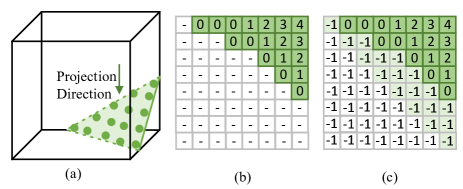
Fig. 2: Illustration of the depth map filling process: (a) the original 3D points in a voxel, (b) the original depth map, (c) the modified depth map, where the depth of empty pixels is labeled with “-1”. Only the depths of green pixels are reconstructed based on the mode index in depth decoding. Furthermore, the depth value of -1 is automatically filtered out.

2 Review of Previous Work

V-PCC [1] and G-PCC [2] mean “video-based point cloud compression” and “geometry-based point cloud compression”, respectively. They are both standards developed by MPEG. V-PCC targets the coding of dense point clouds. It uses a 3D-to-2D projection that projects 3D points onto points in a 2D plane to yield a 2D geometry/occupancy maps. The latter is then encoded by the HEVC video codec [11]. G-PCC aims at coding sparse point clouds and it adopts an octree scheme to encode the 3D coordinates of points.

Motivated by the success of deep-learning-based (DL-based) image coding [12, 13], researchers have applied the end-to-end optimized Auto-Encoder (AE) to point cloud compression in [5, 6, 7]. They use 3D CNN or sparse convolution-based AEs to represent the 3D occupancy model of voxelized point cloud geometry data. Inter-block and inter-sequence correlations are extracted via block-based point cloud training. DL-based methods exhibit state-of-the-art coding performance at the expense of very high computational costs and model sizes. The sparse convolution operator was proposed in [14] to reduce the model size. Yet, several inherent problems still exist (e.g., symmetric complexity of encoders/decoders, one model for one bitrate.)

We attempt to leverage the advantages of V-PCC and learning-based codes in the design of GPCGC. On one hand, GPCGC uses projection to reduce the sparsity of points in the 3D space and map them into a 2D plane. On the other hand, GPCGC encodes projected maps hierarchically with a low-complexity learning-based method. For the latter, we revisit VQ. The VQ technique can trace back to 80s [15]. Recent VQ studies include: gain-shape VQ (called Daala) [16, 17], multi-grid multi-block-size VQ (MGBVQ) [18], and the green image codec (GIC) [19, 20]. Since VQ provides a low-complexity learning-based solution, we adopt it in the proposed GPCGC method.

3 GPCGC Method

The proposed GPCGC method consists of two main modules: 1) octree split and projection and 2) depth map coding, as shown in Fig. 1. In the first module, a voxelized input point cloud scan is split and projected under an octree structure. Its output is a set of projected depth maps. In the second module, depth maps are coded by Green Image Codec Units (GICUs). These two modules are elaborated in Sec. 3.1 and Sec. 3.2, respectively.

3.1 Module 1: Octree Split and Projection

Octree Split. Unlike V-PCC which decomposes a point cloud into connected patches and generates global atlas maps, GPCGC adopts a voxelization step that splits an input point cloud set into 3D coarse-to-fine voxels hierarchically. A parent voxel can be split into 8 child voxels by partitioning its side along the $x$, $y$, and $z$ axes into two halves. A recursive split operation can yield an octree representation. An octree can be non-symmetric; namely, some branches can go to a finer voxel level while others can stay at a coarser level. The coarsest voxel number is $N_{x}\times N_{y}\times N_{z}$, where $N_{x}$, $N_{y}$, and $N_{z}$ are user-selected parameters. The split level can be determined by the rate-distortion optimization technique as discussed in Sec. 3.3. The projection from 3D spatial coordinates of a point to its 2D coordinates is only conducted at each leaf node of the octree. This is the first major difference between our scheme and V-PCC.

Projection. By comparing orthographic projections along the $x$-, $y$-, or $z$-axes, we choose the one that has the largest projection area. To measure the area, we discretize the projected 2D plane with a uniform grid of $p\times p=p^{2}$ blocks. If a block does not contain any projected point, its value is set to zero. Otherwise, its value is set to one. The projection area is defined to be the total number of blocks whose value is equal to one. The distances between 3D points in a leaf voxel and the selected projection plane define a depth map. A larger project area is preferred since the corresponding depth map is flatter and easier to encode. The depth map is also called a depth image. The projection direction at each leaf voxel is coded and included in the bitstream.

Projection Ambiguity Resolution. It is desirable that one block has only one projected point. If this is the case, we can use the block center location and the quantized depth to represent the corresponding 3D point. However, we may encounter two projection ambiguity problems. First, we may see self-occlusions and hidden surfaces in a coarse voxel. For this case, the voxel should be further split into 8 child voxels. This process continues until such problems are resolved or the minimum voxel size is reached. Second, two or more points are projected to the same 2D blocks. The “thickness” concept is introduced to handle the situation. That is, we generate two depth maps to store the maximum and minimum distance values. V-PCC treats the two maps as a two-frame video to exploit of the inter-frame coding of HEVC. We concatenate two maps into a larger map for coding in GPCGC.

3.2 Module 2: Block Occupancy and Depth Coding

Block Occupancy Coding. Some blocks in a geometry map may have no projected points. V-PCC encodes the occupancy map losslessly. It is expensive. To save the bit rate, we adopt a lossy coding scheme. It classifies block occupancy patterns into full-occupied and 8 half-occupied cases (namely left/right, up/down, up-left/lower-right, and up-right/lower-left), leading to 9 modes. We encode the optimal mode that gives the best approximation to the underlying pattern at each leaf node and include it in the bit stream. One example is given in Fig. 2, where we choose the upper-right triangle mode and fill empty blocks with dummy depth value “-1” to simplify the depth encoding/decoding procedure. After depth decoding, only the depths of green pixels are reconstructed based on the mode index and the dummy depth value is automatically filtered out. When the range of depth value lies in $[0,D_{\max}]$, the dummy depth value is set to $-1$ or $D_{\max}+1$ so as to maintain a smooth depth map defined on a squared region.

The lossy coding of block occupancy allows a very small bit rate but could introduce distortion. This is the second major difference between our scheme and V-PCC. The depth value of an empty block that is surrounded by non-empty blocks partially or fully can be inferred from the value of its nearest non-empty block (or the averaged value if there are multiple ones). This is equivalent to adding a new point to the point cloud set. The occupancy distortion can be mitigated by such a process.

Depth Coding. Since a depth map is fundamentally a gray-scale image, it can be coded by any image codec such as JPEG, H.264-Intra, HEVC-Intra. We adopt a low-complexity learning-based image codec known as the GIC method [19]. Its complexity is significantly lower than HEVC-Intra, which meets our low complexity requirement. However, its coding gain is worse than that of HEVC-Intra. The poorer coding gain can be compensated by the effectiveness of block occupancy coding as described above. It is shown in Sec. 4 that the RD performance of our GPCGC is comparable with V-PCC.

GIC downsamples an input image into several spatial resolutions from fine-to-coarse grids and computes image residuals between two adjacent grids. Then, it encodes the coarsest content, interpolates content from coarse-to-fine grids, encodes residuals, and adds residuals to interpolated images for reconstruction. All coding steps are implemented by VQ while all interpolation steps are conducted by the Lanczos interpolation. To facilitate VQ codebook training, a data-driven transform, called the Saab transform [21, 22] is applied for energy compaction and, thus, dimension reduction. We can express the whole GIC framework as the cascade of multiple GIC units, where each GIC unit (GICU) is applied at a fixed grid level. The structure of each GICU is shown in the right of Fig. 1. This is the third major difference between our scheme and V-PCC.

3.3 Rate Control via RDO

We revisit the octree decomposition problem in Module 1. Suppose no projection problem is encountered. A larger voxel size demands a lower coding bit rate but has a higher distortion. The rate-distortion optimization (RDO) technique is used to determine the optimal split. The RDO cost function can be expressed as

$$C_{n}=D_{n}+\lambda_{n}R_{n},$$ (1)

where $C_{n}$, $D_{n}$, $R_{n}$, and $\lambda_{n}$ denote the cost, the bit rate, the distortion, and the Lagrangian multiplier at the $n$th split, respectively.

Rate Modeling. The bit rate is mainly determined by VQ’s coding indices. Let $R_{n}$ denote the total number of bits to encode the depth map at the $n$th split level. Then, we have

$$R_{n}=\sum_{i}\log_{2}{C_{n,i}},$$ (2)

where $C_{n,i}$ is the codebook size of the $i$th grid GICU at the $n$th split level.

Distortion Modeling. V-PCC uses depth coding distortion to evaluate the local distortion. Here, we use the point-to-point Hausdorff distance to measure the local distortion:

$$D_{n}=\max(\cfrac{1}{N_{P1}}\sum_{i}\lVert E(i,j)\rVert^{2},\cfrac{1}{N_{P2}}\sum_{j}\lVert E(j,i)\rVert^{2}),$$ (3)

where $P1$ and $P2$ denote the input and reconstructed point cloud sets at the $n$ split, $i$ and $j$ are points of $P1$ and $P2$, respectively, and $\lVert E(i,j)\rVert^{2}$ is the Hausdorff distance between points $i$ and $j$.

To allow various trade-offs between $R_{n}$ and $D_{n}$, we can adjust $\lambda_{n}$ flexibly. The value of $\lambda_{n}$ is larger for a smaller $n$. This is different from end-to-end DL-based coding methods that have a fixed $\lambda$ in the loss function. We compare the two cost functions, $C_{n}$ and $C_{n+1}$, and choose the optimal one. The RDO process is the fourth major difference between our scheme and V-PCC.

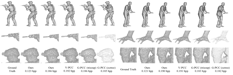
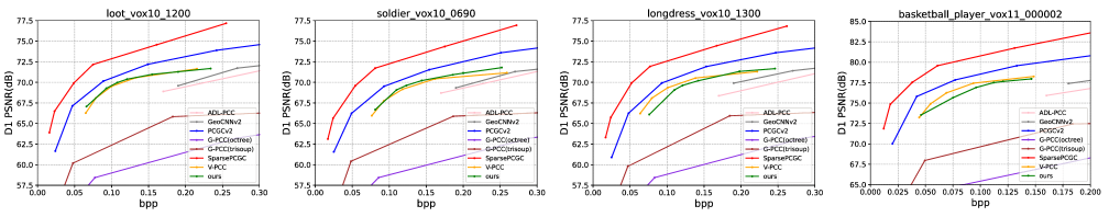
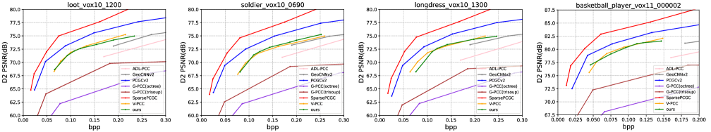
Fig. 3: Visual Comparison of soldier_vox10_0690 and loot_vox10_1200: the whole PC view and two zoom-in views (from top to bottom) of ground truth, GPCGC at two bitrates, V-PCC, G-PCC (trisoup), and G-PCC (octree) (from left to right).

Fig. 4: RD Performance comparison of eight coding methods: V-PCC, G-PCC (octree), G-PCC (trisoup), ADL-PCC, GeoCNNv2, PCGCv2, SparsePCGC, and GPCGC (ours).

4 Experiments

Experimental Setup. The coarsest input voxel size is 32x32x32. The split number ranges from $n=0$ to $3$. When $n=3$, the voxel size is 4x4x4. The Lagrangian multipliers, $\lambda_{n}$, in Eq. (2) are empirically set to $\lambda_{3}=\lambda$, $\lambda_{2}=2.5\lambda$, $\lambda_{1}=4.6\lambda$, $\lambda_{0}=8.0\lambda$. The coding bit rate is controlled by $\lambda$. We use mesh models from ShapeNet [23] and SHREC’19 [24] as the training data. They are converted to point clouds by uniform sampling and voxelized on a 512x512x512 occupancy space. Then, point clouds are split into cubes of various sizes (e.g., 32x32x32, 16x16x16, 8x8x8, and 4x4x4). 20,000 cubes are selected to train our model, and each GICU is trained by 2000 samples on average. The training process is implemented from coarse to fine grids. The VQ module in the GICU is trained using the faiss.KMeans method [25]. The testing set includes single frames from the 8iVFB [26] and the Owlii [27] point cloud datasets. The experiment follows the MPEG Common Test Condition [28].

Performance Analysis. We compare our codec with seven other codecs: V-PCCv18.0 with HM video encoder[29] , G-PCCv14.0 (trisoup)[30], G-PCCv14.0 (octree)[30], ADL-PCC [6], GeoCNNv2 [9], PCGCv2 [14], and SparsePCGC [10]. The last four are DL-based methods. The bit rate is calculated using bits per input point (bpp). We use the BD-rate to evaluate the coding performance. The distortion metrics are the mean-squared error (MSE) of the point-to-point (p2point or D1) and the point-to-plane (p2plane or D2) distances. Their RD curves for four test sequences are shown in Fig. 4. We categorize the eight methods based on their RD performance from the best to the worst RD into four groups: 1) SparsePCGC and PCGCv2, 2) GPCGC (ours) and V-PCC, 3) GeoCNNv2 and ADL-PCC, and 4) G-PCC (trisoup) and G-PCC (octree). Although there is a performance gap between our codec and two state-of-the-art DL methods, SparsePCGC and PCGCv2, the model size and complexity of our codec are significantly lower than those of the two as discussed below. Two coded point cloud sets and their zoom-in views of GPCGC, V-PCC, G-PCC (trisoup), and G-PCC (octree) are shown in Fig. 4 for visual comparison. Our method offers a smooth transition from a higher bit rate (i.e., 0.18bpp) to a lower bit rate (i.e., 0.12bpp) in terms of subjective quality.

Model Size and Complexity Analysis. We compare the model size and the encoding/decoding floating-point operations (FLOPs) of the top four performers (i.e., SparsePCGC, PCGCv2, V-PCC, and our GPCGC) in Table 1. V-PCC is not a learning-based codec. Its model size is negligible. Our method can handle multiple coding rates with a single model. It has a size of 0.33 million parameters. In contrast, DL-based codecs need multiple models to handle multiple bit rates. The table only lists the size of one model. If there are $K$ models in the model zoo, the actual model sizes are $0.78\times K$ and $2.88\times K$ million parameters for PCGCv2 and SparsePCGC, respectively.

The encoding/decoding FLOPs are computed under the following setting. The input point clouds are voxelized into 1024x1024x1024 voxels. The occupancy ratios of the vox10 test sequences range from 0.071% to 0.101% with an average value of 0.084%. For V-PCC, we use the Intel VTune software to measure their FLOPs in the geometry coding process over the same sequences with 10-bit precision. For DL-based methods, we make an estimation based on their network structure. We report the averaged encoding/decoding FLOPs in the last two columns of Table 1. As shown in the table, our codec has 4G and 64M FLOPs on average for the encoding and decoding of a point cloud set, respectively. In comparison, DL-based methods have significantly higher encoding/decoding complexity. Their decoding complexities are about 1000x of ours. Moreover, the encoding/decoding FLOPs of our codec are smaller than those of V-PCC. The savings are 60% and 64%, respectively. We should point out that FLOPs only account for a very small percentage of micro-Operations in traditional codecs such as V-PCC and G-PCC. If we take the non-floating-point operations into account, our codec has even more significant savings in complexity. The low FLOPs of our decoder come from the simple structure of GIC [19]. Only look-up tables are required for VQ decoding and some matrix multiplications are needed for the inverse-Saab transform.

Methods	Model Size	Enc FLOPs	Dec FLOPs
PCGCv2	0.78M	17.5G	60G
SparsePCGC	2.88M	35G	100G
V-PCC	-	10G	180M
GPCGC (ours)	0.33M	4G	64M

Table 1: Comparison of the model sizes and the complexity in terms of the encoding/decoding floating-point operations (FLOPs) of four benchmarking codecs.

5 Conclusion

A low-complexity point cloud geometry compression method, called the Green Point Cloud Geometry Codec (GPCGC), was proposed. The novel contributions include projection on octree-decomposed voxels, lossy occupancy map coding, GICU-based depth map coding, and RDO for bit rate control. The last one is difficult to achieve in DL-based codecs. As compared with MPEG V-PCC, GPCGC achieves lower encoding/decoding complexity (with a saving of around 60%) while maintaining a comparable coding gain. As compared with DL-based models, GPCGC has significantly smaller model parameters and lower encoding/decoding complexity. The low-complexity advantage of GPCGC comes from the multi-resolution depth map coding with GICU, which consists of the Saab transform and VQ. We plan to develop a green coding solution for dynamic point clouds as an extension in the future.

References

- [1] MPEG, “V-pcc codec description,” ISO/IEC JTC 1/SC 29/WG 7 N00100, 2020.
- [2] MPEG, “G-pcc codec description v12,” ISO/IEC JTC 1/SC 29/WG 7 N00151, 2021.
- [3] S. Schwarz, M. Preda, V. Baroncini, M. Budagavi, P. Cesar, P. A. Chou, R. A. Cohen, M. Krivokuća, S. Lasserre, Z. Li, J. Llach, K. Mammou, R. Mekuria, O. Nakagami, E. Siahaan, A. Tabatabai, A. M. Tourapis, and V. Zakharchenko, “Emerging mpeg standards for point cloud compression,” IEEE Journal on Emerging and Selected Topics in Circuits and Systems, vol. 9, no. 1, pp. 133–148, 2019.
- [4] D. Graziosi, O. Nakagami, S. Kuma, A. Zaghetto, T. Suzuki, and A. Tabatabai, “An overview of ongoing point cloud compression standardization activities: Video-based (v-pcc) and geometry-based (g-pcc),” APSIPA Transactions on Signal and Information Processing, vol. 9, p. e13, 2020.
- [5] M. Quach, G. Valenzise, and F. Dufaux, “Learning convolutional transforms for lossy point cloud geometry compression,” in 2019 IEEE International Conference on Image Processing (ICIP), 2019, pp. 4320–4324.
- [6] A. F. R. Guarda, N. M. M. Rodrigues, and F. Pereira, “Adaptive deep learning-based point cloud geometry coding,” IEEE Journal of Selected Topics in Signal Processing, vol. 15, no. 2, pp. 415–430, 2021.
- [7] J. Wang, H. Zhu, H. Liu, and Z. Ma, “Lossy point cloud geometry compression via end-to-end learning,” IEEE Transactions on Circuits and Systems for Video Technology, vol. 31, no. 12, pp. 4909–4923, 2021.
- [8] T. M. Borges, D. C. Garcia, and R. L. De Queiroz, “Fractional super-resolution of voxelized point clouds,” IEEE Transactions on Image Processing, vol. 31, pp. 1380–1390, 2022.
- [9] M. Quach, G. Valenzise, and F. Dufaux, “Improved deep point cloud geometry compression,” in 2020 IEEE 22nd International Workshop on Multimedia Signal Processing (MMSP), 2020, pp. 1–6.
- [10] J. Wang, D. Ding, Z. Li, X. Feng, C. Cao, and Z. Ma, “Sparse tensor-based multiscale representation for point cloud geometry compression,” IEEE Transactions on Pattern Analysis and Machine Intelligence, pp. 1–18, 2022.
- [11] G. J. Sullivan, J.-R. Ohm, W.-J. Han, and T. Wiegand, “Overview of the high efficiency video coding (hevc) standard,” IEEE Transactions on circuits and systems for video technology, vol. 22, no. 12, pp. 1649–1668, 2012.
- [12] D. P. Kingma, M. Welling et al., “An introduction to variational autoencoders,” Foundations and Trends® in Machine Learning, vol. 12, no. 4, pp. 307–392, 2019.
- [13] J. Ballé, D. Minnen, S. Singh, S. J. Hwang, and N. Johnston, “Variational image compression with a scale hyperprior,” arXiv preprint arXiv:1802.01436, 2018.
- [14] J. Wang, D. Ding, Z. Li, and Z. Ma, “Multiscale point cloud geometry compression,” in 2021 Data Compression Conference (DCC), 2021, pp. 73–82.
- [15] R. Gray, “Vector quantization,” IEEE Assp Magazine, vol. 1, no. 2, pp. 4–29, 1984.
- [16] J.-M. Valin and T. B. Terriberry, “Perceptual vector quantization for video coding,” in Visual Information Processing and Communication VI, vol. 9410. SPIE, 2015, pp. 65–75.
- [17] J.-M. Valin, N. E. Egge, T. Daede, T. B. Terriberry, and C. Montgomery, “Daala: A perceptually-driven still picture codec,” in 2016 IEEE International Conference on Image Processing (ICIP). IEEE, 2016, pp. 76–80.
- [18] Y. Wang, Z. Mei, I. Katsavounidis, and C.-C. J. Kuo, “Lightweight image codec via multi-grid multi-block-size vector quantization (mgbvq),” arXiv preprint arXiv:2209.12139, 2022.
- [19] Y. Wang, Z. Mei, Q. Zhou, I. Katsavounidis, and C.-C. J. Kuo, “Green image codec: a lightweight learning-based image coding method,” in Applications of Digital Image Processing XLV, vol. 12226. SPIE, 2022, pp. 70–75.
- [20] C.-C. J. Kuo and A. M. Madni, “Green learning: Introduction, examples and outlook,” Journal of Visual Communication and Image Representation, p. 103685, 2022.
- [21] C.-C. J. Kuo, M. Zhang, S. Li, J. Duan, and Y. Chen, “Interpretable convolutional neural networks via feedforward design,” Journal of Visual Communication and Image Representation, vol. 60, pp. 346–359, 2019.
- [22] Y. Chen, M. Rouhsedaghat, S. You, R. Rao, and C.-C. J. Kuo, “Pixelhop++: A small successive-subspace-learning-based (ssl-based) model for image classification,” in 2020 IEEE International Conference on Image Processing (ICIP). IEEE, 2020, pp. 3294–3298.
- [23] A. X. Chang, T. Funkhouser, L. Guibas, P. Hanrahan, Q. Huang, Z. Li, S. Savarese, M. Savva, S. Song, H. Su et al., “Shapenet: An information-rich 3d model repository,” arXiv preprint arXiv:1512.03012, 2015.
- [24] R. M. Dyke, C. Stride, Y.-K. Lai, P. L. Rosin, M. Aubry, A. Boyarski, A. M. Bronstein, M. M. Bronstein, D. Cremers, M. Fisher, T. Groueix, D. Guo, V. G. Kim, R. Kimmel, Z. Lähner, K. Li, O. Litany, T. Remez, E. Rodolà, B. C. Russell, Y. Sahillioğlu, R. Slossberg, G. K. L. Tam, M. Vestner, Z. Wu, and J. Yang, “Shape correspondence with isometric and non-isometric deformations,” in Eurographics Workshop on 3D Object Retrieval, S. Biasotti, G. Lavoué, and R. Veltkamp, Eds. The Eurographics Association, 2019.
- [25] J. Johnson, M. Douze, and H. Jégou, “Billion-scale similarity search with gpus,” IEEE Transactions on Big Data, vol. 7, no. 3, pp. 535–547, 2019.
- [26] E. d’Eon, B. Harrison, T. Myers, and P. A. Chou, “8i voxelized full bodies-a voxelized point cloud dataset,” ISO/IEC JTC1/SC29 Joint WG11/WG1 (MPEG/JPEG) input document WG11M40059/WG1M74006, vol. 7, no. 8, p. 11, 2017.
- [27] Y. Xu, Y. Lu, and Z. Wen, “Owlii dynamic human textured mesh sequence dataset,” in ISO/IEC JTC1/SC29/WG1 1 input document m41658, 2017.
- [28] D. Group et al., “Common test conditions for point cloud compression,” ISO/IEC JTC1/SC29/WG11 Doc. N18474, 2019.
- [29] MPEG, “Mpeg-pcc-tmc2 (v18.0),” 2022. [Online]. Available: https://github.com/MPEGGroup/mpeg-pcc-tmc2
- [30] MPEG, “mpeg-pcc-tmc13 (v14.0),” 2021. [Online]. Available: https://github.com/MPEGGroup/mpeg-pcc-tmc13