Single Proxy Control

Abstract

Negative control variables are sometimes used in non-experimental studies to detect the presence of confounding by hidden factors. A negative control outcome (NCO) is an outcome that is influenced by unobserved confounders of the exposure effects on the outcome in view, but is not causally impacted by the exposure. Tchetgen Tchetgen (2013) introduced the Control Outcome Calibration Approach (COCA) as a formal NCO counterfactual method to detect and correct for residual confounding bias. For identification, COCA treats the NCO as an error-prone proxy of the treatment-free counterfactual outcome of interest, and involves regressing the NCO on the treatment-free counterfactual, together with a rank-preserving structural model which assumes a constant individual-level causal effect. In this work, we establish nonparametric COCA identification for the average causal effect for the treated, without requiring rank-preservation, therefore accommodating unrestricted effect heterogeneity across units. This nonparametric identification result has important practical implications, as it provides single proxy confounding control, in contrast to recently proposed proximal causal inference, which relies for identification on a pair of confounding proxies. For COCA estimation we propose three separate strategies: (i) an extended propensity score approach, (ii) an outcome bridge function approach, and (iii) a doubly-robust approach. Finally, we illustrate the proposed methods in an application evaluating the causal impact of a Zika virus outbreak on birth rate in Brazil.

Keywords: Confounding Proxy; Doubly Robust; Extended Propensity Score; Negative Controls; Unmeasured Confounding.

1 Introduction

Unmeasured confounding is a well-known threat to valid causal inference from observational data. An approach that is sometimes used in practice to assess residual confounding bias, is to check whether known null effects can be recovered free of bias, by evaluating whether the exposure or treatment of interest is found to be associated with a so-called negative control outcome (NCO), upon adjusting for measured confounders (Rosenbaum, 1989; Lipsitch et al., 2010; Shi et al., 2020). An observed variable is said to be a valid negative control outcome or more broadly, an outcome confounding proxy, to the extent that it is associated with hidden factors confounding the exposure-outcome relationship in view, although not directly impacted by the exposure. Therefore, an NCO which is empirically associated with the exposure, might suggest the presence of residual confounding. In the event such an association is present, a natural question is whether the negative control outcome can be used for bias correction. The most well-established NCO approach for debiasing observational causal effect estimates is the difference-in-differences approach (DiD) (Card and Krueger, 1994; Lechner, 2011; Caniglia and Murray, 2020). In fact, DiD may be viewed as directly leveraging the pre-treatment outcome as an NCO since it cannot logically be causally impacted by the treatment. Identification then follows from an additive equi-confounding assumption that the unmeasured confounder association with the post-treatment outcome of interest matches that with the pre-treatment outcome on the additive scale (Sofer et al., 2016). The baseline outcome in DiD is thus implicitly assumed to be a valid NCO, and equi-confounding is equivalent to the so-called parallel trends assumption, that the average trends in treatment-free potential outcomes for treatment and untreated units are parallel. In practice, equi-confounding or equivalently parallel trends may not be reasonable for a number of reasons, including if the outcome trend is also impacted by an unmeasured common cause with the treatment. Furthermore, additive equi-confounding may not be realistic as a broader debiasing method in non-DiD settings where the NCO is not necessarily a pre-treatment measurement of the outcome of interest, but is instead a post-treatment measurement of a different type of outcome (and might therefore have support on a different scale than the outcome of interest has). To address these potential limitations of additive equi-confounding, Tchetgen Tchetgen (2013) introduced the Control Outcome Calibration Approach (COCA) as a simple yet formal counterfactual NCO approach to debias causal effect estimates in observational analyses. At its core, COCA essentially treats the NCO variable as a proxy measurement for the treatment-free potential outcome, which therefore is associated with the latter, and which becomes independent of the treatment assignment mechanism, upon conditioning on the treatment-free counterfactual outcome. As the treatment-free potential outcome can be viewed as an ultimate source of unmeasured confounding, this assumption formalizes the idea that, as a relevant proxy for the source of residual confounding, the NCO would be made irrelevant for the treatment assignment mechanism if one were to hypothetically condition on the underlying potential outcome.

For identification and inference for a continuous outcome, the original COCA approach of Tchetgen Tchetgen (2013) involves the correct specification of a regression model for the NCO, conditional on the treatment-free potential outcome and measured confounders, together with a rank-preserving structural model which effectively assumes a constant individual-level treatment effect. In this paper, we develop a nonparametric COCA identification framework for the average causal effect for the treated, which equally applies irrespective of the nature of the primary outcome, whether binary, continuous, or polytomous. Importantly, as we show, the proposed COCA identification framework completely obviates the need for rank preservation, therefore accommodating an arbitrary degree of effect heterogeneity across units. Relatedly, an alternative counterfactual approach named proximal causal inference has recently developed in causal inference literature (Miao et al., 2016, 2018; Tchetgen Tchetgen et al., 2020), which leverages a pair of negative treatment and outcome control variables, or more broadly treatment and outcome confounding proxies, to nonparametrically identify treatment causal effects subject to residual confounding without invoking a rank-preservation assumption. Importantly, while proximal causal inference relies on two proxies for causal identification, in contrast, COCA is a single-proxy control approach which therefore may present practical advantages. For estimation and inference, we introduce three strategies to implement COCA which improve on prior methods: (i) an extended propensity score approach, (ii) a so-called outcome calibration bridge function approach, and (iii) a doubly robust approach which carefully combines approaches (i) and (ii) and remains unbiased for the effect of treatment on the treated, provided that either approach is also unbiased, without necessarily knowing which method might not be unbiased. Finally, we illustrate the methods with an application evaluating the causal effect of a Zika outbreak on birth rate in Brazil, and we conclude with possible extensions to our methods and a brief discussion.

2 Notation and Brief Review of COCA

Consider an observational study where, as represented in Figure 1, one has observed an outcome variable $Y$, a binary treatment $A$ whose causal effect on $Y$ is of interest, and measured pre-treatment covariates $X$. We are concerned that as displayed succinctly in the figure with the bow arc, the association between $A$ and $Y$ is confounded by hidden factors.

Figure 1: A Graphical Illustration of A Simple Causal Model

Throughout, $Y^{a}$ denotes the potential outcome or counterfactual, had possibly contrary to fact, the exposure been set to $a$ by an external hypothetical intervention. Furthermore, throughout, we also make the consistency assumption:

Assumption 1

$Y=Y^{a=A}$.

Hereafter, we aim to make inferences about the causal effect of treatment on the treated (ETT), denoted by $\psi^{*}=E\big{(}Y^{a=1}-Y^{a=0}|A=1\big{)}$. Under consistency, $\psi_{1}^{*}=E\big{(}Y^{a=1}|A=1\big{)}$ is identified by $E\big{(}Y|A=1\big{)}$; to identify the counterfactual mean $\psi_{0}^{*}=E\big{(}Y^{a=0}|A=1\big{)}$ requires additional assumptions. Standard methods often resort to the no unmeasured confounding assumption, i.e., $Y^{a=0}\,\rotatebox[origin={c}]{90.0}{$\models$}\,A\,\big{|}\,X$, a strong assumption we do not make. Instead, we suppose that one has measured a valid NCO $W$, possibly multi-dimensional, which is known a priori to satisfy the following conditions:

Assumption 2

Condition (i): $W^{a}=W$ for all $a=0,1$, where $W^{a}$ is the potential NCO under an external intervention that sets $A=a$; Condition (ii): $W\not\rotatebox[origin={c}]{90.0}{$\models$}\,Y^{a=0}\,\big{|}\,X$; Condition (iii): $W\,\rotatebox[origin={c}]{90.0}{$\models$}\,A\,\big{|}\,(Y^{a=0},X)$.

Assumption 2-(i) encodes the key assumption of a known null causal effect of the treatment on the NCO in potential outcome notation. Assumption 2-(ii) encodes that $W$ is relevant for predicting the treatment-free potential outcome of interest. Assumption 2-(iii) states that $W$ is independent of $A$ conditional on treatment-free potential outcome and covariates. These conditions formally encode the assumption that $W$ is a valid proxy for the treatment-free potential outcome, a source of residual confounding bias; $W$ is only associated with the treatment mechanism to the extent that it is associated with the confounding mechanism captured by the potential outcome. We illustrate these NCO assumptions with the causal graph displayed in Figure 2. The thick arrows in the graph indicate the deterministic relationship defining the observed outcome in terms of potential outcomes and treatment variables by the consistency assumption. The missing arrows on the graph formally encode the core conditional independence conditions implied by Assumption 2.

Figure 2: A Graphical Illustration of the Assumptions for Control Outcome Calibration Approach. Thick arrows depict the deterministic relationship between $Y$ and $(Y^{a=1},Y^{a=0},A)$, as established by the consistency assumption (Assumption 1).

It is enlightening to consider a data generating mechanism that is compatible with Assumption 2. As an example, we consider the following latent variable model for a continuous outcome:

$$Y^{a=0}=h(U,X)\ ,$$ (1a)

$$W\not\rotatebox[origin={c}]{90.0}{$\models$}\,U\,\big{|}\,X\text{ and }W\,\rotatebox[origin={c}]{90.0}{$\models$}\,A\,\big{|}\,(U,X)$$ (1b)

where $U$ is a continuously distributed unobserved variable and $h(u,x)$ is a function that is strictly monotone in $u$ for all $x$, but otherwise completely unrestricted. In Appendix A.1, we establish that expressions (1a)-(1b) imply Assumption 2. Expression (1a) means that the treatment-free outcome is a monotonic transformation of an unobserved variable $U$, an instance of a so-called changes-in-changes model (Athey and Imbens, 2006). Expression (1b) corresponds to Assumption 2-(ii) and (iii). Of note, if $W$ has a deterministic relationship with $(U,X)$, say $W=h_{w}(U,X)$ where $h_{w}(u,x)$ varies in $u$ (potentially non-monotonic), (1b) is satisfied. Figure 3 provides a graphical representation compatible with, although not exclusive, expressions (1a)-(1b).

Figure 3: A Graphical Illustration of a Structural Model Compatible with (1). Measured covariates $X$ are suppressed for simplicity. The thick arrows depict the deterministic relationships $Y^{a=0}=h(U)$ and $Y=Y^{A}$.

For identification and estimation in the case of a continuous outcome, Tchetgen Tchetgen (2013) further assumed the rank-preserving structural model:

$$Y=Y^{a=0}+\psi^{*}A,$$ (2)

which by consistency, implies a constant individual-level causal effect $\psi^{*}=Y^{a=1}-Y^{a=0}$. Under this model, he noted that upon defining $Y(\psi)=Y-\psi A$, then one can deduce from Assumption 2 that $W\,\rotatebox[origin={c}]{90.0}{$\models$}\,A\,\big{|}\,(Y(\psi),X)$ if and only if $\psi=\psi^{*}$, in which case, given equation (2), $Y^{a=0}=Y(\psi^{*})=Y-\psi^{*}A$ which motivates a regression-based implementation of COCA, that entails searching for the parameter value of $\psi=\psi^{*}$ such that $E\big{\{}W|A,Y(\psi),X\big{\}}=E\big{\{}W|Y(\psi),X\big{\}}$. A straightforward implementation of the approach uses linear models whereby for each value of $\psi$ on a sufficiently fine grid, one obtains an estimate of the regression model $E\big{\{}W|Y(\psi),X\big{\}}=\beta_{1}+\beta_{2}A+\beta_{3}Y(\psi)+\beta_{4}X$ using ordinary least squares (OLS), with estimated coefficients $\big{(}\widehat{\beta}_{1}(\psi),\widehat{\beta}_{2}(\psi),\widehat{\beta}_{3}(\psi),\widehat{\beta}_{4}(\psi)\big{)}$. Then a 95% confidence interval for $\psi^{*}$ consists of all values of $\psi$ for which a valid test of the null hypothesis $\beta_{2}(\psi)=0$ fails to reject at the 0.05 type 1 error level.  Such hypothesis test might be performed by verifying whether the interval $\widehat{\beta}_{2}(\psi)\pm 1.96\widehat{\mathrm{SE}}\big{(}\widehat{\beta}_{2}(\psi)\big{)}$ covers $0,$ with $\widehat{\mathrm{SE}}\big{(}\widehat{\beta}_{2}(\psi)\big{)}$ the OLS estimate of the standard error of $\widehat{\beta}_{2}(\psi)$. Tchetgen Tchetgen (2013) also describes a potentially simpler one-shot approach which fits a single regression $E\big{(}W|A,Y,X\big{)}=\beta_{1}+\beta_{2}^{*}A+\beta_{3}Y+\beta_{4}X$ via OLS where $\beta_{2}^{*}=-\beta_{3}/\psi_{0},$ in which case $\widehat{\psi}=-\widehat{\beta}_{2}^{*}/\widehat{\beta}_{3}$ where $\big{(}\widehat{\beta}_{2}^{*},\widehat{\beta}_{3}\big{)}$ are OLS estimates; a corresponding standard error estimator of $\widehat{\psi}$ is given in Section A.2 of the Appendix for convenience. Though practically convenient, validity of either approach relies on both correct specification of the linear model for $W$ given $(Y^{a=0},X)$, and on the rank-preserving structural model, which may be biologically implausible. In the following, we describe alternative methods aimed at addressing these limitations.

3 Identification of the Effect of Treatment on the Treated

3.1 Identification via Extended Propensity Score Weighting

In order to establish identification, consider the extended propensity score function (EPS):

$$\pi^{*}\big{(}y,x\big{)}=\Pr\big{(}A=1\,\big{|}\,Y^{a=0}=y,X=x\big{)}$$

which makes explicit the fact that in presence of unmeasured confounding, the treatment mechanism will generally depend on the treatment-free potential outcome. For notational brevity, we define the treatment odds $\omega^{*}(y,x)=\pi^{*}(y,x)/\{1-\pi^{*}(y,x)\}$. Since $\omega^{*}$ and $\pi^{*}$ have a one-to-one relationship, we use $\omega^{*}$ throughout to model the exposure mechanism. We assume that the positivity holds, i.e.,

Assumption 3

For all $(y,x)$, we have $0<\omega^{*}(y,x)<\infty$, i.e., $0<\pi^{*}(y,x)<1$.

Next, we note that were $\omega^{*}$ known, identification of the average treatment-free potential outcome in the treated would then be empirically identified by the expression

$$\psi_{0}^{*}=\frac{E\big{\{}\big{(}1-A\big{)}Y\omega^{*}\big{(}Y,X\big{)}\big{\}}}{E\big{\{}\big{(}1-A\big{)}\omega^{*}\big{(}Y,X\big{)}\big{\}}}\ .$$ (3)

See Appendix B.1 for the details. Therefore, the average causal effect of treatment on the treated would be identified by

$$\psi^{*}=E\big{(}Y|A=1\big{)}-\frac{E\big{\{}\big{(}1-A\big{)}Y\omega^{*}\big{(}Y,X\big{)}\big{\}}}{E\big{\{}\big{(}1-A\big{)}\omega^{*}\big{(}Y,X\big{)}\big{\}}}\ .$$ (4)

As the exposure mechanism $\omega^{*}$ is unknown, we next demonstrate how the NCO assumption can be leveraged to identify the latter quantity. Let $p\big{(}w,x\big{)}=\Pr\big{(}A=1|W=w,X=x\big{)}$. The proposed approach to identify $\omega^{*}$ is based on the following equality, which we prove in Appendix B.2:

Result 1

Under Assumptions 1-3, we the following result almost surely:

$$\frac{p\big{(}W,X\big{)}}{1-p\big{(}W,X\big{)}} =E\left\{\omega^{*}(Y,X)\,\big{|}\,W,X,A=0\right\}=\sum_{y}\frac{\pi^{*}\big{(}y,X\big{)}}{1-\pi^{*}\big{(}y,X\big{)}}g\big{(}y|W,X,A=0\big{)}$$ (5)

where $p\big{(}y\,\big{|}\,W,X,A=0\big{)}$ is the conditional law of $Y$ given $(W,X,A)$ evaluated at $Y=y$.

Result 1 provides an expression relating the exposure mechianism of interest to the observed data distribution, as of the three quantities involved in the expression $p,g$ and $\omega^{*}$; two are uniquely determined by the observed data, mainly $p$ and $g$, which are then related to the unknown function of interest $\omega^{*}$ in Result 1; see the Appendix A.3 for a graphical illustration. Equation (5) is known as an integral equation, more precisely a Fredholm integral equation of the first kind. We then have the following identification result.

Result 2

If Assumptions 1-3 hold, and the integral equation (5) in Result 1 admits a unique solution, then $\omega^{*}$ and $\pi^{*}$ are nonparametrically identified from the observed data by solving (5), and $\psi_{0}^{*}$ is nonparametrically identified by (3).

Sufficient conditions for the existence and uniqueness of a solution to such an equation are well-studied by mathematicians; see Section A.5 for details. Such conditions were recently discussed by statisticians in the context of proximal causal inference (Miao et al., 2016, 2018; Tchetgen Tchetgen et al., 2020), a recently proposed alternative approach for bias correction leveraging a pair of negative control variables or proxy variables. A detailed comparison of COCA with proximal causal inference is relegated to Section 6. Intuitively, the condition that the integral equation admits a unique solution essentially requires that $W$ is sufficiently relevant for $Y^{a=0}$ in the sense that for any variation in the latter, there is corresponding variation in the former. This assumption is akin to the assumption of relevance in the context of instrumental variable methodology, which states that variation in the instrument should induce variation in the treatment. Importantly, Result 2 applies whether $Y$ is binary, continuous or polytomous, provided that $W$ is sufficiently relevant for $Y^{a=0}$, to ensure that equation (3) admits a solution. Also, the result obviates the need for a rank-preserving structural model, and delivers fully nonparametric identification of the causal effect of treatment on the treated.

3.2 Identification via COCA Confounding Bridge Function

In this Section, we introduce an alternative nonparametric identification and estimation approach which does not rely on modeling the EPS, but instead relies on the existence of a so-called confounding bridge function. In order to make progress, we make the following assumption.

Assumption 4

For any $y$, there exists a function (possibly nonlinear) $b^{*}(w,x)$ that satisfies the following equation

$$y=E\left\{b^{*}\big{(}W,X\big{)}\,\big{|}\,Y=y,X=x,A=0\right\}.$$ (6)

Intuitively, upon noting that under Assumptions 1-2, Assumption 4 can equivalently be stated in terms of potential outcomes

$$Y^{a=0}=E\left\{b^{*}\big{(}W,X\big{)}|Y^{a=0},X\right\}$$ (7)

which essentially formalizes the idea that $W$ is a sufficiently relevant proxy for the potential outcome $Y^{a=0}$ if there exist a (possibly unknown) transformation of $(W,X)$ whose conditional expectation given $(Y^{a=0},X)$, recovers $Y^{a=0}$. As $b^{*}(W,X)$ provides a bridge between the observed data equation (6), and its potential outcome counterpart (7), we aptly refer to $b^{*}\big{(}W,X\big{)}$ as a COCA confounding bridge function. Note that classical measurement error is a special case of the equation in the display above in which case $b^{*}$ is the identity map and $W=Y^{a=0}+e$ where $e$ is an independent mean zero error. The condition can therefore be viewed as nonparametric generalization of classical measurement error which allows $W$ and $Y$ to be of arbitrary nature and does not assume the error to be unbiased on the additive scale. We further illustrate the assumption in the case of binary $W$ and $Y$. As shown in Appendix B.4, in this case with suppressing covariates, the following $b^{*}(W)$ satisfies (6):

$$b^{*}(W)=\frac{-(1-W)\cdot\Pr\big{(}W=1|Y=0,A=0\big{)}+W\cdot\Pr\big{(}W=0|Y=0,A=0\big{)}}{\Pr\big{(}W=1|Y=1,A=0\big{)}-\Pr\big{(}W=1|Y=0,A=0\big{)}};$$

provided that $\Pr\big{(}W=1|Y^{a=0}=1\big{)}\not=\Pr\big{(}W=1|Y^{a=0}=0\big{)}$, encoding the requirement that $W$ cannot be independent of $Y^{a=0}$, i.e., Assumption 2. Beyond the binary case, for more general outcome types, Assumption 4 likewise formally defines a Fredholm integral equation of the first kind, for which sufficient conditions for existence of a solution are well characterized in functional analysis textbooks; we again refer the reader to Miao et al. (2016). We are now ready to state our result, which we prove in Appendix B.5:

Result 3

Suppose that Assumptions 1-4 hold, and $b^{*}$ satisfies (6). Then,

$$\psi_{0}^{*}=E\big{\{}b^{*}\big{(}W,X\big{)}\,\big{|}\,A=1\big{\}}\ \text{ and }\ \psi^{*}=E\big{\{}Y-b^{*}(W,X)\,\big{|}\,A=1\big{\}}\ .$$ (8)

In the binary example discussed above where $b^{*}(w)$ was uniquely identified, we have that

$$\psi_{0}^{*} =E\left\{b^{*}\big{(}W\big{)}|A=1\right\}=\frac{\Pr\big{(}W=1|A=1\big{)}-\Pr\big{(}W=1|Y=0,A=0\big{)}}{\Pr\big{(}W=1|Y=1,A=0\big{)}-\Pr\big{(}W=1|Y=0,A=0\big{)}}\ .$$

We briefly highlight a key feature of the above result reflected in its proof, which is that $b^{*}\big{(}W,X\big{)}$ need not be uniquely identified by equation (6), and that any such solution leads to a unique value for $E\big{(}Y^{a=0}|A=1\big{)}.$ Interestingly, the identifying formula in the display above was also obtained by Tchetgen Tchetgen (2013) in the binary case, although he did not emphasize the key role of the bridge function as a general framework for identification beyond the binary case.

3.3 Identification via an Influence Function

In this Section, we characterize an influence function for the ETT $\psi^{*}$. Let a model $\mathcal{M}$ be a collection of observed data laws that admit a solution to (6), i.e.,

$$\mathcal{M}=\Bigg{\{}P\,\Bigg{|}\,\begin{array}[]{l}\text{$P(O)$ is regular and Assumption \ref{condition-1} holds,}\\ \text{i.e., there exists $b^{*}$ solving \eqref{Outcome COCA}}\end{array}\Bigg{\}}\ .$$

We further consider the following subjectivity condition:

• (Surjectivity): Let $T:\mathcal{L}_{2}(W,X)\rightarrow\mathcal{L}_{2}(Y,A=0,X)$ denote the operator given by $T(g)=E\big{\{}g(W,X)\,\big{|}\,Y,A=0,X\big{\}}$. At the true data law, $T$ is surjective.

The surjectivity condition states that the Hilbert space $\mathcal{L}_{2}(W,X)$ is sufficiently rich so that any elements in $\mathcal{L}_{2}(Y,A=0,X)$ can be recovered via the conditional expectation mapping; see Cui et al. (2023), Dukes et al. (2023), and Ying et al. (2023) for related discussions. In addition, we consider a submodel $\mathcal{M}_{\text{sub}}$:

$$\mathcal{M}_{\text{sub}}=\Bigg{\{}P\in\mathcal{M}\,\Bigg{|}\,\begin{array}[]{l}\text{$\omega^{*}$ and $b^{*}$ are unique solutions to \eqref{EPS equation} and \eqref{Outcome COCA}, respectively, }\\ \text{and \hyperlink{(Surjectivity)}{(Surjectivity)} is satisfied}\end{array}\Bigg{\}}$$

We then establish the semiparametric local efficiency bound for $\psi^{*}$ under model $\mathcal{M}$ at submodel $\mathcal{M}_{\text{sub}}$.

Result 4

Suppose Assumptions 1-4 hold. The following results hold.

• The following function $\texttt{IF}(O;\omega^{*},b^{*})$ is an influence function for $\psi^{*}$ under model $\mathcal{M}$.

  $$\texttt{IF}(O;\omega^{*},b^{*})=\frac{A\big{\{}Y-b^{*}\big{(}W,X\big{)}-\psi^{*}\big{\}}-(1-A)\omega^{*}(Y,X)\left\{Y-b^{*}\big{(}W,X\big{)}\right\}}{\Pr\big{(}A=1\big{)}}\ .$$ (9)

• The influence function $\texttt{IF}(O;\omega^{*},b^{*})$ is the efficient influence function for $\psi^{*}$ under model $\mathcal{M}$ at submodel $\mathcal{M}_{\text{sub}}$. Therefore, the corresponding semiparametric local efficiency bound for $\psi^{*}$ is $Var\big{\{}\texttt{IF}(O;\omega^{*},b^{*})\big{\}}$.

The influence function IF resembles the influence function for $\psi^{*}$ in the proximal causal inference framework; see Section G of Cui et al. (2023) for details. Interestingly, the influence function has the following doubly robust property (Scharfstein et al., 1999; Lunceford and Davidian, 2004; Bang and Robins, 2005); see Appendix B.6 for the proof:

Result 5

Suppose that Assumptions 1-4 are satisfied. In addition, suppose that either (i) $E\big{\{}b^{\dagger}\big{(}W,X\big{)}\,\big{|}\,A=0,Y=y,X\big{\}}=y$ or (ii) $\omega^{\dagger}\big{(}y,x\big{)}=\omega^{*}\big{(}y,x\big{)}$, but not necessarily both, is satisfied. Then, we have that $E\big{\{}\texttt{IF}(O;\omega^{\dagger},b^{\dagger})\big{\}}=0$.

In words, if either the COCA confounding bridge function or the EPS, but not necessarily both, is correctly specified, the influence function is an unbiased estimating function of $\psi^{*}$.

Using expressions (3), (8), and (9), one can construct parametric estimators of $\psi^{*}$. Specifically, the first estimator using (3) entails a priori specifying a parametric model for the EPS, say a logistic regression model. The second estimator based on (8) entails a priori specifying a parametric model for the COCA bridge function, say a linear model. Lastly, the third estimator based on (9) entails parametric models for both EPS and COCA bridge function. The first two estimators rely on the correct exposure and COCA bridge function specifications, respectively. Thus, misspecification of either model will likely result in biased inferences about the ETT. On the other hand, the last estimator has a doubly-robust property (Scharfstein et al., 1999; Lunceford and Davidian, 2004; Bang and Robins, 2005) in that it can be used for unbiased inference about the ETT if either EPS or COCA bridge function is correct, without a priori knowledge of which model if any is incorrect. In Section A.4, we provide details of constructing these three parametric estimators and their large sample behavior.

A significant limitation of the three parametric estimators is their dependence on specific parametric specifications of nuisance components, which can lead to biased inference if the model specifications are incorrect. To address this concern, a potential solution is to develop an estimator where nuisance components are estimated using nonparametric methods, drawing on advancements in recent learning theory. In the following Section, we construct such an estimator and study its statistical properties.

4 A Semiparametric Locally Efficient Estimator

Our estimator is derived from the influence function IF in Result 5 and adopted the cross-fitting approach (Schick, 1986; Chernozhukov et al., 2018), which is implemented as follows. We randomly split $N$ study units, denoted by $\mathcal{I}=\{1,\ldots,N\}$, into $K$ non-overlapping folds, denoted by $\{\mathcal{I}_{1},\ldots,\mathcal{I}_{K}\}$. For each $k=1,\ldots,K$, we estimate the EPS and COCA confounding bridge function using observations in $\mathcal{I}_{k}^{c}=\mathcal{I}\setminus\mathcal{I}_{k}$, and then evaluate the estimated nuisance functions using observations in $\mathcal{I}_{k}$ to obtain an estimator of $\psi^{*}(a_{Y},a_{D})$. We refer to $\mathcal{I}_{k}^{c}$ and $\mathcal{I}_{k}$ as the estimation and evaluation folds, respectively. To use the entire sample, we take the simple average of the $K$ estimators.

We introduce the following additional notation in order to facilitate the discussion. Let $\mathcal{H}(V)$ be the Reproducing Kernel Hilbert Space (RKHS) of $V$ endowed with the Gaussian kernel $\mathcal{K}$, i.e., $\mathcal{K}(v,v^{\prime})=\exp\big{\{}-\big{\|}v-v^{\prime}\|_{2}^{2}/\kappa\big{\}}$ where $\kappa\in(0,\infty)$ is a bandwidth parameter. For each $k=1,\ldots,K$, let $\mathbbm{P}^{(-k)}(V)=|\mathcal{I}_{k}^{c}|^{-1}\sum_{i\in\mathcal{I}_{k}^{c}}V_{i}$ and $\mathbbm{P}^{(k)}(V)=|\mathcal{I}_{k}|^{-1}\sum_{i\in\mathcal{I}_{k}}V_{i}$.

We estimate the EPS and COCA bridge functions by adopting a recently developed minimax estimation approach (Ghassami et al., 2022). We remark that other approaches (e.g., Mastouri et al. (2021)) can also be adopted with minor modifications. Note that the true weight function $\omega^{*}(Y,X)$ and the true COCA confounding bridge function $b^{*}(W,X)$ satisfy

$$E\left[\big{\{}(1-A)\omega^{*}(Y,X)-A\big{\}}p\big{(}W,X\big{)}\right]=0\ ,\ \forall p\in\mathcal{L}_{2}(W,X)\ ,$$

$$E\left[(1-A)\big{\{}Y-b^{*}(W,X)\big{\}}q(Y,X)\right]=0\ ,\ \forall q\in\mathcal{L}_{2}(Y,X)\ .$$

Therefore, following Ghassami et al. (2022), minimax estimators of $\omega^{*}$ and $b^{*}$ are given by

$$\widehat{\omega}^{(-k)}(\cdot)$$

$$=\operatorname*{arg\,min}_{\omega\in\mathcal{H}(Y,X)}\Bigg{[}\displaystyle{\max_{p\in\mathcal{H}(W,X)}}\Bigg{[}\mathbbm{P}^{(-k)}\Big{[}p(W,X)\big{\{}(1-A)\omega(Y,X)-A\big{\}}-p^{2}(W,X)\Big{]}-\lambda_{p}\big{\|}p\big{\|}_{\mathcal{H}}^{2}\Bigg{]}+\lambda_{\omega}\big{\|}\omega\big{\|}_{\mathcal{H}}^{2}\Bigg{]}$$

$$\widehat{b}^{(-k)}(\cdot)$$

$$=\operatorname*{arg\,min}_{h\in\mathcal{H}(W,X)}\Bigg{[}\displaystyle{\max_{q\in\mathcal{H}(Y,X)}}\Bigg{[}\mathbbm{P}^{(-k)}\Big{[}q(Y,X)(1-A)\big{\{}Y-b(W,X)\big{\}}-q^{2}(Y,X)\Big{]}-\lambda_{q}\big{\|}q\big{\|}_{\mathcal{H}}^{2}\Bigg{]}+\lambda_{b}\big{\|}b\big{\|}_{\mathcal{H}}^{2}\Bigg{]}$$

where $\big{\|}\cdot\big{\|}_{\mathcal{H}}$ is an RKHS norm and $\lambda\in(0,\infty)$ are regularization parameters.

We make a few remarks about the minimax estimation approach, of which details are relegated to Section A.6 of the Appendix. First, despite the complicated formulas, closed-form representations of $\widehat{\omega}^{(-k)}$ and $\widehat{b}^{(-k)}$ are available from the represented theorem (Kimeldorf and Wahba, 1970; Schölkopf et al., 2001). Second, the bandwidth parameters $\kappa$ and the regularization parameters $\lambda$ can be chosen from cross-validation. Lastly, $\omega^{*}$ may vary widely because it is a ratio of two probabilities. In such cases, the proposed minimax estimator may result in significantly small or negative estimates. To mitigate this issue, one may consider a practical approach to regularize the minimiax estimator when it appears to be ill-behaved.

Using the minimax estimators of the nuisance functions, a semiparametric estimator $\widehat{\psi}$ of $\psi^{*}$ is then obtained as follows:

$$\widehat{\psi}=\frac{1}{K}\sum_{k=1}^{K}\widehat{\psi}^{(k)}\ ,$$

$$\widehat{\psi}^{(k)}=\frac{\frac{1}{N}\sum_{i=1}^{N}A_{i}Y_{i}-\mathbbm{P}^{(k)}\big{[}(1-A)\widehat{\omega}^{(-k)}(Y,X)\big{\{}Y-\widehat{b}^{(-k)}(W,X)\big{\}}+A\widehat{b}^{(-k)}(W,X)\big{]}}{\frac{1}{N}\sum_{i=1}^{N}A_{i}}\ .$$

Under regularity conditions, the semiparametric estimator $\widehat{\psi}$ is consistent and asymptotically normal for $\psi^{*}$. To proceed, we introduce the following notation. For a function $g(O)$, let $\big{\|}g\big{\|}_{P,2}=\big{[}E\big{\{}g^{2}(O)\big{\}}\big{]}^{1/2}$ be the $L_{2}(P)$-norm of $g$.

Assumption 5

Suppose the following conditions hold for all $k=1,\ldots,K$:

• (Boundedness) There exists a finite constant $C>0$ such that

  $$\big{|}\omega^{*}(y,x)\big{|}\in[C^{-1},C]\ ,\quad\big{|}\widehat{\omega}^{(-k)}(y,x)\big{|}\in[C^{-1},C]\quad\text{ for all $(y,x)$,}$$

  $$\big{|}b^{*}(w,x)\big{|}\leq C\ ,\quad\big{|}\widehat{b}^{(-k)}(w,x)\big{|}\leq C\quad\text{ for all $(w,x)$,}\quad E(Y^{4})\leq C\ .$$

• (Consistency) As $N\rightarrow\infty$, we have $\big{\|}\widehat{\omega}^{(-k)}-\omega^{*}\big{\|}_{P,2}=o_{P}(1)$ and $\big{\|}\widehat{b}^{(-k)}-b^{*}\big{\|}_{P,2}=o_{P}(1)$.

• (Cross-product Rates) As $N\rightarrow\infty$, we have

  $$\min\Bigg{[}\begin{array}[]{l}\big{\|}\widehat{\omega}^{(-k)}-\omega^{*}\big{\|}_{P,2}\big{\|}E^{(-k)}\big{[}(1-A)\big{\{}b^{*}(W,X)-\widehat{b}^{(-k)}(W,X)\big{\}}\,\big{|}\,Y,X\big{]}\big{\|}_{P,2},\\ \big{\|}\widehat{b}^{(-k)}-b^{*}\big{\|}_{P,2}\big{\|}E^{(-k)}\big{[}(1-A)\big{\{}\omega^{*}(Y,X)-\widehat{\omega}^{(-k)}(Y,X)\big{\}}\,\big{|}\,W,X\big{]}\big{\|}_{P,2}\end{array}\Bigg{]}=o_{P}(N^{-1/2})\ .$$

Assumption 5-(i) states that nuisance functions and the corresponding estimators are uniformly bounded. Assumption 5-(ii) states that the estimated nuisance functions are consistent for the true nuisance functions in the $L_{2}(P)$ norm sense. Assumption 5-(iii) states that the cross-product rate of nuisance function estimators are $o_{P}(N^{-1/2})$. Importantly, if one nuisance function is estimated at sufficiently fast rates, the other nuisance function is allowed to converge at a substantially slower rate provided that the cross-products remain $o_{P}(N^{-1/2})$. This is an instance of the mixed-bias property described by Rotnitzky et al. (2020); Ghassami et al. (2022). It is also worth highlighting the structure of the mixed bias in the current context which is the minimum of two product biases, each containing a bias term for a nuisance function and a projected bias term for the other nuisance function; this property was first reported in Ghassami et al. (2022) for a large class of functionals including ours.

Result 6 establishes that $\widehat{\psi}$ is consistent and asymptotically normal (CAN) for $\psi^{*}$.

Result 6

Suppose Assumptions 1-5 hold. Then, we have $\sqrt{N}\big{(}\widehat{\psi}-\psi^{*}\big{)}\stackrel{{\scriptstyle D}}{{\rightarrow}}N(0,\sigma^{2})$ where $\sigma^{2}=Var\big{\{}\texttt{IF}(O;\omega^{*},b^{*})\big{\}}$. Moreover, a consistent estimator of $\sigma^{2}$ is $\widehat{\sigma}^{2}=\sum_{k=1}^{K}\widehat{\sigma}^{2,(k)}/K$ where

$$\widehat{\sigma}^{2,(k)}=\frac{\mathbbm{P}^{(k)}\big{[}\big{[}A\big{\{}Y-\widehat{b}^{(-k)}\big{(}W,X\big{)}-\widehat{\psi}^{(k)}\big{\}}-\big{(}1-A\big{)}\widehat{\omega}^{(-k)}(Y,X)\big{\{}Y-\widehat{b}^{(-k)}\big{(}W,X\big{)}\big{\}}\big{]}^{2}\big{]}}{\big{(}\sum_{i=1}^{N}A_{i}/N\big{)}^{2}}\ .$$

Using the variance estimator $\widehat{\sigma}^{2}$, valid $100(1-\alpha)$% confidence intervals for the ATT are given by $\big{(}\widehat{\psi}+z_{\alpha/2}\widehat{\sigma}/\sqrt{N},\widehat{\psi}+z_{1-\alpha/2}\widehat{\sigma}/\sqrt{N}\big{)}$ where $z_{\alpha}$ is the $100\alpha$th percentile of the standard normal distribution. Alternatively, one may construct confidence intervals using the multiplier bootstrap; see Section A.6 for details.

Lastly, the cross-fitting estimator depends on a specific sample split, and thus, may produce outlying estimates if some split samples do not represent the entire data. To mitigate this issue, Chernozhukov et al. (2018) proposes to use median adjustment from multiple cross-fitting estimates; the detail can be found in the Appendix A.6.

5 Data Application: Zika Virus Outbreak in Brazil

The Zika virus, which can be transmitted from a pregnant woman to her fetus, can cause serious brain abnormalities, including microcephaly (i.e., an abnormally small head) (Rasmussen et al., 2016). Brazil is one of the countries hardest hit by the Zika virus. In particular, the outbreak in 2015 resulted in over 200,000 cases in Brazil by 2016 (Lowe et al., 2018). As a result, many prior works (Castro et al., 2018; Diaz-Quijano et al., 2018; Taddeo et al., 2022; Tchetgen Tchetgen et al., 2023) asked whether the Zika virus outbreak caused a drop in birth rates.

We re-analyzed the dataset analyzed in Taddeo et al. (2022) and Tchetgen Tchetgen et al. (2023). In the dataset, we focused on 673 municipalities in two states of Brazil, Pernambuco and Rio Grande do Sul, which are northeastern and southernmost states. Out of the 1248 cases of microcephaly that occurred in Brazil by November 28, 2015, 51.8% (646 cases) were reported in Pernambuco (PE), less than 10 cases of Zika-related microcephaly were reported in Rio Grande do Sul (RS) (Gregianini et al., 2017), which shows that PE was severely impacted by the Zika virus outbreak, while RS was minimally affected. Based on their epidemiologic histories, we defined 185 and 488 municipalities in PE and RS as treated and control groups, respectively.

For each municipality, we included the following variables in the analysis. As pre-treatment covariates, we included municipality-level population size, population density, and proportion of females measured in 2014. We used the post-epidemic municipality-level birth rate in 2016 as the outcome $Y$, where the birth rate is defined as the total number of live human births per 1,000 persons. We used the pre-epidemic municipality-level birth rates in 2013 and 2014 as the outcome proxies (i.e., NCO), denoted by $W_{1}$ and $W_{2}$, respectively. To be valid proxies, the birth rates in 2013 and 2014 must satisfy the Assumption 2 conditions: (i) birth rates in 2013 and 2014 cannot be causally impacted by the Zika virus epidemic which occurred in 2015, (ii) birth rates in 2013 and 2014 are correlated with what the birth rate in 2016 would have been had there not been a Zika virus epidemic, and (iii) birth rates in 2013 and 2014 are independent of a municipality’s Zika epidemic status, upon conditioning on its Zika virus epidemic-free potential birth rate in 2016. The first two conditions are uncontroversial, while the third condition largely relies on the extent to which pre-epidemic birth rates can accurately be viewed as a proxy for the counterfactual birth rate had the pandemic not occurred, and as such would not further be predictive of whether the municipality experienced a high rate of Zika virus incidence, conditional on the region’s epidemic-free counterfactual birth rate in 2016. Although one might consider this last assumption reasonable, ultimately, it is empirically untestable without making an alternative assumption. Nevertheless, in the Appendix A.8, we describe a straightforward sensitivity analysis to evaluate the extent to which violation of the assumption might impact inference.

Using the dataset, we estimated $\psi^{*}=E\big{(}Y^{a=1}-Y^{a=0}\,\big{|}\,A=1\big{)}$, i.e., the difference between the observed average birth rate of Pernambuco and a forecast of what it would have been had the Zika outbreak been prevented. Therefore, the ETT quantifies the average treatment effect of the Zika outbreak on the birth rate within the Pernambuco region. Of note, the crude estimand $E(Y\,\big{|}\,A=1)-E(Y\,\big{|}\,A=0)$ was estimated to be equal to $3.384$, suggesting that municipalities in the PE region (with higher incidence of Zika virus) experienced a higher birth rate than RS regions in 2016 during the Zika virus outbreak. An immediate concern is that this crude association between $A$ and $Y$ might be subject to significant confounding bias, leading us to conduct two separate analyses geared at addressing residual confounding bias; the proposed COCA methods, which we compared with a standard difference-in-differences analysis. Thus, we estimate the ETT using the approach outlined in Section 4 where the NCOs are specified as either (i) $W_{1}$, birth rate in 2013, or (ii) $W_{2}$, birth rate in 2014, or (iii) $(W_{1},W_{2})$. For comparison, we also obtained doubly-robust parametric estimators of the ETT using the three NCO specifications; see the Appendix A.7 for details on how these estimators were constructed.

Table 1 summarizes corresponding results. We find that the six COCA estimates vary between $-1.833$ and $-2.410$, meaning between $1.833$ and $2.410$ birth per 1,000 persons were reduced in PE due to the Zika virus outbreak, an empirical finding better aligned with the scientific hypothesis that Zika may likely adversely impact the birth rates of exposed populations. Compared to the crude estimate of 3.384, the negative effect estimates indeed provide compelling evidence of potential confounding. We also obtain an estimate using the difference-in-difference estimator under a standard parallel trends assumption (e.g., Card and Krueger (1994); Angrist and Pischke (2009)), which yields a considerably smaller effect estimate varying between $-1.156$ and $-1.041$; noting that the DiD estimator requires the assumption of equi-confounding of the $A-Y$ association in the pre- and post-periods, while our proposed estimator does not (but instead requires conditions (i)-(iii) outlined above). Regardless of the estimator, all estimates appear to be consistent with the anticipated adverse causal impact of the Zika Virus epidemic. Consequently, we conclude that based on inferences aimed at accounting for confounding (DiD and COCA), the Zika virus outbreak likely led to a decline in the birthrate of affected regions in Brazil, which agrees with similar findings in the literature (Castro et al., 2018; Diaz-Quijano et al., 2018; Taddeo et al., 2022; Tchetgen Tchetgen et al., 2023).

Estimator	Statistic	NCO
		$W_{1}$	$W_{2}$	$(W_{1},W_{2})$
Semiparametric COCA	Estimate	$-2.410$	$-2.182$	$-2.180$
	SE	$0.356$	$0.503$	$0.342$
	95% CI	($-3.107$,$-1.713$)	($-3.168$,$-1.196$)	($-2.850$,$-1.510$)
Doubly-robust parametric COCA	Estimate	$-2.235$	$-1.833$	$-2.182$
	SE	$0.502$	$0.519$	$0.415$
	95% CI	($-3.220$,$-1.250$)	($-2.850$,$-0.816$)	($-2.996$,$-1.368$)
Standard DiD under parallel trends	Estimate	$-1.156$	$-1.041$	$-1.041$
	SE	$0.199$	$0.195$	$0.195$
	95% CI	($-1.546$,$-0.767$)	($-1.424$,$-0.658$)	($-1.424$,$-0.658$)

Table 1: Summary of Data Analysis. Values in “Estimate” row represent the estimates of the ETT. Values in “SE” and “95% CI” rows represent the standard errors (SEs) associated with the estimates and the corresponding 95% confidence intervals (CIs), respectively. The reported values are expressed as births per 1,000 persons.

6 Discussion and Possible Extensions

We have described a COCA nonparametric identification framework, therefore extending previous results of Tchetgen Tchetgen (2013) to a more general setting accommodating outcomes of arbitrary nature and obviating the need for an assumption of constant treatment effects, i.e. rank preservation. We have proposed three estimation strategies including a doubly robust method which has appealing robustness properties. Interestingly, the COCA central identifying assumption, that conditioning on the treatment-free counterfactual would in principle shield the treatment assignment from any association with the NCO is isomorphic to an analogous assumption in the missing data literature where an outcome might be missing not at random; however, a fully observed so-called shadow variable (the missing data analog of an NCO) reasonably assumed to be conditionally independent of the missing data process given the value of the potentially missing outcome. For example, Zahner et al. (1992) considered a study of the children’s mental health evaluated through their teachers’ assessments in Connecticut. However, the data for the teachers’ assessments are subject to nonignorable missingness. As a proxy of the teacher’s assessment, a separate parent report is available for all children in this study. The parent report is likely to be correlated with the teacher’s assessment, but is unlikely to be related to the teacher’s response rate given the teacher’s assessment and fully observed covariates. Hence, the parental assessment is regarded as a shadow variable for the teacher’s assessment in this study. The literature on shadow variables is fast-growing (d’Haultfoeuille, 2010; Kott, 2014; Wang et al., 2014; Miao et al., 2015; Miao and Tchetgen Tchetgen, 2016; Li et al., 2021), the methods developed in this paper have close parallels to shadow variable counterparts in this literature. This connection to shadow variables is particularly salient when the COCA confounding bridge function is not uniquely defined, which can easily occur for instance when the shadow variable (or analogously the NCO) is multivariate, therefore significantly complicating inference. Fortunately, the methods developed by Li et al. (2021) for the analogous shadow variable setting directly apply to the corresponding COCA setting and thus provides a complete solution for identification and inference for the average treatment effect for the treated without relying on completeness conditions nor on unique identification of either the EPS or the COCA confounding bridge function. We refer the interested reader to this latter work for further details. It is worth noting that the doubly robust estimator proposed in this paper appears to be completely new, and different from those of Miao et al. (2015); Miao and Tchetgen Tchetgen (2016); Li et al. (2021) and therefore may also be of use in shadow variable applications. Likewise, the doubly robust estimators proposed in the latter works can equally be applied to the current COCA setting as an alternative inferential approach.

Additionally, as mentioned in the previous Section, the key assumption that conditioning on the treatment-free potential outcome, would in principle make the NCO or outcome proxy irrelevant to treatment mechanism is ultimately untestable, and may in certain settings not hold exactly. In fact, this would be the case if the NCO were in fact explicitly used in assigning the treatment in which case the assumption might be violated. In order to address such eventuality, the analyst might consider several candidate proxies/NCOs when available, and may even perform an over-identification test, by inspecting the extent to which the estimated causal effect depends on the choice of proxy. Alternatively, a sensitivity analysis might also be performed to evaluate the potential impact of a hypothesized departure from the assumption. In the context of the Zika virus application, an over-identification test and a sensitivity analysis were carried out as illustrative examples, with the corresponding results and discussion provided in the Appendix A.8 and A.9.

Finally, as previously mentioned in the Introduction, COCA offers an alternative approach to proximal causal inference (Miao et al., 2016; Tchetgen Tchetgen et al., 2020) for debiasing observational estimates of the effect of treatment on the treated by leveraging negative control or valid confounding proxies. A key difference highlighted earlier between these two frameworks is that COCA relies on a single valid NCO which directly proxies the treatment-free potential outcome, while proximal causal inference requires both valid NCO and negative control treatment variables that proxy an underlying unmeasured confounder. Importantly, COCA takes advantage of the fact that the treatment-free potential outcome is observed in the untreated, while in proximal causal inference, the unmeasured confounders for which proxies are available, are themselves never observed, arguably a more challenging identification task. Despite the practical advantage of needing one rather than two proxies, it is important to note that though COCA identifies the effect of treatment on the treated, it fails to nonparametrically identify the population average treatment effect (ATE), identified by proximal causal inference, without an additional assumption. In contrast, proximal causal inference provides nonparametric identification of both causal parameters and thus can be interpreted as providing richer identification opportunities. A key reason for this difference in the scope of identification is the fact that in the current paper, we have emphasized an interpretation of the NCO as a proxy for the treatment-free potential outcome but not for the potential outcome under treatment, in the sense that under our conditions, it must be that the treatment-free potential outcome does not only shield the treatment from the NCO, but also shields the potential outcome under treatment from the latter. Two potential strategies to recover COCA identification of the population ATE, might be either (i) evoke a rank-preservation assumption which if appropriate would imply that the ETT and the ATE are equal (this is the assumption made in Tchetgen Tchetgen (2013)); or (ii) identify a second proxy NCO which is a valid proxy for the counterfactual outcome under treatment. The second condition would be needed if $Y^{a=1}$ can also be viewed as a hidden confounder. By a symmetry argument, one can show that (ii) in fact would provide identification of the average counterfactual outcome under treatment for the untreated. A weighted average of both counterfactual means would then provide identification of the ATE. Details are not provided, but can easily be deduced from the presentation.

7 Acknowledgment

The authors would like to thank Jamie Robins, Thomas Richardson and Ilya Shpitser for helpful discussions.

Supplementary Material

This document provides details of “Single Proxy Control.” In Section A, we provide details of the main paper. In Section B, we provide proofs of the results in the main paper.

Appendix A Details of the Main Paper

A.1 Details of the Latent Variable Model (1)

Recall that model (1) is given by

$$Y^{a=0}=h(U,X)\ ,\ h(u,x):\text{strictly increasing in $u$ for all $x$}$$ (1a)

$$W\not\rotatebox[origin={c}]{90.0}{$\models$}\,U\,\big{|}\,X\text{ and }W\,\rotatebox[origin={c}]{90.0}{$\models$}\,A\,\big{|}\,(U,X)$$ (1b)

Under these assumptions, we establish that

$$W\not\rotatebox[origin={c}]{90.0}{$\models$}\,U\,\big{|}\,X\quad\Rightarrow\quad W\not\rotatebox[origin={c}]{90.0}{$\models$}\,h^{-1}(Y^{a=0},X)\,\big{|}\,X\quad\Rightarrow\quad W\not\rotatebox[origin={c}]{90.0}{$\models$}\,Y^{a=0}\,\big{|}\,X$$

justifying Assumption 2-(ii): $W\not\rotatebox[origin={c}]{90.0}{$\models$}\,Y^{a=0}\,\big{|}\,X$, and

$$W\,\big{|}\,(U=u,A=1,X)\stackrel{{\scriptstyle D}}{{=}}W\,\big{|}\,(U=u,A=0,X)$$

$$\Rightarrow\quad W\,\big{|}\,(h^{-1}(Y^{a=0},X)=u,A=1,X)\stackrel{{\scriptstyle D}}{{=}}W\,\big{|}\,(h^{-1}(Y^{a=0},X)=u,A=0,X) (\because\ \text{$h$ is monotonic})$$

$$\Rightarrow\quad W\,\big{|}\,(Y^{a=0}=h(u,X),A=1,X)\stackrel{{\scriptstyle D}}{{=}}W\,\big{|}\,(Y^{a=0}=h(u,X),A=0,X) (\because\ \text{Definition of $Y^{a=0}$})$$

$$\Rightarrow\quad W\,\big{|}\,(Y^{a=0}=y,A=1,X)\stackrel{{\scriptstyle D}}{{=}}W\,\big{|}\,(Y^{a=0}=y,A=0,X)$$

justifying Assumption 2-(iii): $W\,\rotatebox[origin={c}]{90.0}{$\models$}\,A\,\big{|}\,(Y^{a=0},X)$.

A.2 Standard Error of the COCA Estimator in Tchetgen Tchetgen (2013)

We provide details on the standard error of the COCA estimator obtained from the ordinary least squares estimators of the regression model $E(W|A,Y,X)=\beta_{1}+\beta_{2}^{*}A+\beta_{3}Y+\beta_{4}X$. It is well known that the variance estimator of the OLS estimator $(\widehat{\beta}_{1},\widehat{\beta}_{2}^{*},\widehat{\beta}_{3},\widehat{\beta}_{4})$ is given as

$$\widehat{V}:=\widehat{\sigma}^{2}\left[\sum_{i=1}^{N}\begin{pmatrix}1&A_{i}&Y_{i}&X_{i}\\ A_{i}&A_{i}^{2}&A_{i}Y_{i}&A_{i}X_{i}\\ Y_{i}&A_{i}Y_{i}&Y_{i}^{2}&Y_{i}X_{i}\\ X_{i}&A_{i}X_{i}&Y_{i}X_{i}&X_{i}^{2}\end{pmatrix}\right]^{-1}\ ,\ \widehat{\sigma}^{2}:=\frac{\sum_{i=1}^{N}\big{(}W_{i}-\widehat{\beta}_{1}-\widehat{\beta}_{2}^{*}A_{i}-\widehat{\beta}_{3}Y_{i}-\widehat{\beta}_{4}X_{i}\big{)}^{2}}{N-4}$$

where $N$ is the number of observed units, indexed by subscript $i=1,\ldots N$. Let $f(a,b)=a/b$. Then, the first-order Taylor expansion around $(a_{0},b_{0})$ is

$$\frac{a}{b}=f(a,b)\simeq f(a_{0},b_{0})+f_{1}(a_{0},b_{0})(a-a_{0})+f_{2}(a_{0},b_{0})(b-b_{0})=\frac{a_{0}}{b_{0}}+\frac{a-a_{0}}{b_{0}}-\frac{a_{0}(b-b_{0})}{b_{0}^{2}}$$

where $f_{1}(a,b)=\partial f(a,b)/\partial a$ and $f_{2}(a,b)=\partial f(a,b)/\partial b$. Therefore, we find

$$E\big{\{}(\widehat{\psi}_{0}-\widehat{\psi}_{0})^{2}\big{\}} =E\bigg{\{}\bigg{(}\frac{\widehat{\beta}_{2}^{*}}{\widehat{\beta}_{3}}-\frac{{\beta}_{2}^{*}}{{\beta}_{3}}\bigg{)}^{2}\bigg{\}}$$

$$\simeq E\bigg{\{}\bigg{(}\frac{\widehat{\beta}_{2}^{*}-\beta_{2}^{*}}{{\beta}_{3}}-\frac{\beta_{2}^{*}(\widehat{\beta}_{3}-\beta_{3})}{{\beta}_{3}^{2}}\bigg{)}^{2}\bigg{\}}$$

$$=\frac{Var(\widehat{\beta}_{2}^{*})}{\beta_{3}^{2}}-2\frac{\beta_{2}^{*}Cov(\widehat{\beta}_{2}^{*},\widehat{\beta}_{3})}{\beta_{3}^{3}}+\frac{(\beta_{2}^{*})^{2}Var(\widehat{\beta}_{3})}{\beta_{3}^{4}}$$

Consequently, the standard error estimator of $\widehat{\psi}$ is given as $SE_{\psi_{0}}=\widehat{\beta}_{3}^{-1}\Big{(}\widehat{V}_{22}-2\widehat{\psi}_{0}\widehat{V}_{23}+\widehat{\psi}_{0}^{2}\widehat{V}_{33}\Big{)}^{1/2}$ where $\widehat{V}_{ij}$ is the $(i,j)$th element of $\widehat{V}$.

A.3 A Graphical Illustration of Result 1

Recall that Result 1 is given by

$$\frac{p\big{(}W,X\big{)}}{1-p\big{(}W,X\big{)}} =E\left\{\omega^{*}(Y,X)\,\big{|}\,W,X,A=0\right\}=\sum_{y}\frac{\pi^{*}\big{(}y,X\big{)}}{1-\pi^{*}\big{(}y,X\big{)}}g\big{(}y|W,X,A=0\big{)}$$ (5)

where $g\big{(}y\,\big{|}\,W,X,A=0\big{)}$ is the conditional law of $Y$ given $(W,X,A)$ evaluated at $Y=y$. To illustrate, we consider the following data generating process:

• $A\sim\text{Ber}(0.5)$

• $Y^{a=0}\sim N(0.25A,1)$

• $W=Y^{a=0}+\epsilon$ where $\epsilon\sim N(0,1)$ with $\epsilon\,\rotatebox[origin={c}]{90.0}{$\models$}\,(Y^{a=0},A)$

We find the odds function relating $W$ and $A$ and that relating $Y^{a=0}$ and $A$ are given by

$$\text{Odds}(W=w)=\frac{p(w)}{1-p(w)}=\frac{\Pr(A=1\,\big{|}\,W=w)}{\Pr(A=0\,\big{|}\,W=w)}=\frac{\phi(w;0.25,2)}{\phi(w;0,2)}$$

$$\text{Odds}(Y^{a=0}=y)=\frac{\pi^{*}(y)}{1-\pi^{*}(y)}=\frac{\Pr(A=1\,\big{|}\,Y^{a=0}=y)}{\Pr(A=0\,\big{|}\,Y^{a=0}=y)}=\frac{\phi(y;0.25,1)}{\phi(y;0,1)}$$

where $\phi(v;\mu,\sigma^{2})$ is the density of $N(\mu,\sigma^{2})$. In addition, $Y^{a=0}\,\big{|}\,(W,A=0)\sim N(W/2,0.5)$. From straightforward algebra, we find $E\big{\{}\text{Odds}(Y^{a=0})\,\big{|}\,W,A=0\big{\}}=\text{Odds}(W)$. We then generate $N=1000$ observations from the data generating process, and we draw a scatterplot of $\text{Odds}(W_{i})$ and $\text{Odds}(Y_{i}^{a=0})$ in Figure 4.

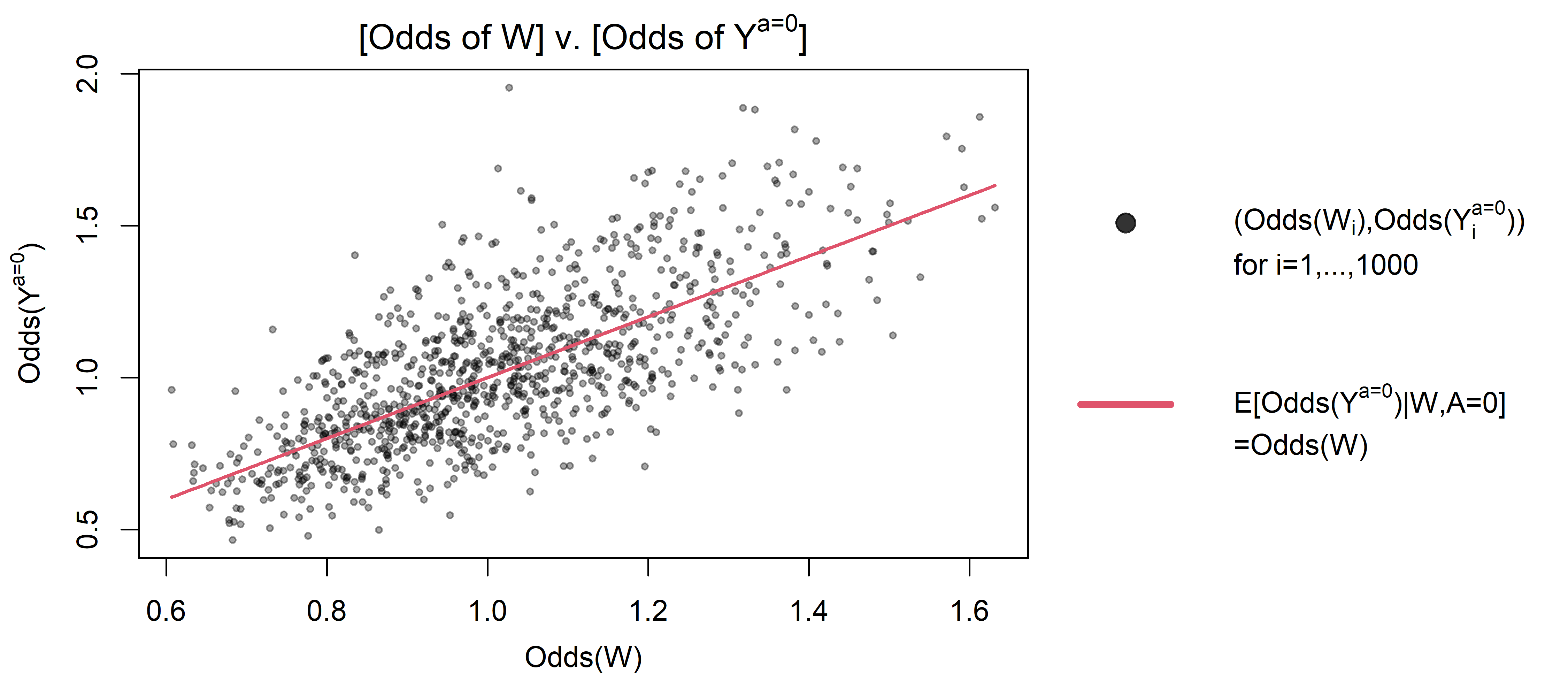
Figure 4: A scatterplot of $\text{Odds}(W_{i})$ and $\text{Odds}(Y_{i}^{a=0})$ for $i=1,\ldots,N$. The red solid line shows the deterministic relationship $\text{Odds}(W=w)=E\{\text{Odds}(Y^{a=0})\,\big{|}\,W=w,A=0\}$.

A.4 Details of the Construction of Parametric Estimators via GMM

In this Section, we provide details of the generalized method of moments (GMM, Hansen (1982)), which is implemented in many publicly available software programs, such as gmm package in R (Chaussé, 2010). Before we present details, we introduce additional notations. Let $N$ be the number of observed units, indexed by subscript $i=1,\ldots N$. Let $O_{i}=(Y_{i},A_{i},W_{i})$ be the observed data for the $i$th unit. Let $\mathbbm{P}(h)$ denote the average of function $h(O)$ across $N$ units, i.e., $\mathbbm{P}(g)=N^{-1}\sum_{i=1}^{N}g(O_{i})$. For random variables $V$ and $Z$, let $V\stackrel{{\scriptstyle D}}{{\rightarrow}}Z$ denote $V$ converges to $Z$ in distribution.

Let $\psi_{1}^{*}=E(Y^{a=1}\,\big{|}\,A=1)$ and $\psi_{0}^{*}=E(Y^{a=0}\,\big{|}\,A=1)$. The additive and multiplicative additive average causal effects of treatment on the treated are represented as $\psi^{*}:=\psi_{1}^{*}-\psi_{0}^{*}$. Let $\theta$ be a vector of parameters of interest and $g$ be a vector-valued function that is restricted by the mean-zero moment restriction, i.e. $E\big{\{}g(O;\theta^{\dagger})\big{\}}=0$ where $\theta^{\dagger}$ is the unique parameter that achieves the mean-zero moment restriction.

A.4.1 A Moment Restriction based on the EPS

The first approach entails a priori specifying a parametric logistic regression model for the EPS, say:

$$\log\omega(y,x;\alpha)=\log\frac{\pi\big{(}y,x;\alpha\big{)}}{1-\pi\big{(}y,x;\mathbf{\alpha}\big{)}}=\mathbf{\alpha}^{\intercal}S_{y}(y,x)\ ,$$

where $S_{y}\big{(}y,x\big{)}$ is a user-specified sufficient statistic for the log-odds ratio ratio association between $Y^{a=0}$ and $A$ evaluated at $Y^{a=0}=y$ given $X=x$. Options for specifying $S_{y}$ includes both more parsimonious specifications, e.g., $S_{y}\big{(}y,x\big{)}=(1,y,x^{\intercal})^{\intercal}$, as well as more flexible specifications, say $S_{y}\big{(}y,x\big{)}=\big{(}1,y,y^{2},\ldots,y^{v},x^{\intercal},yx^{\intercal},\ldots,y^{v}x^{\intercal}\big{)}^{\intercal}$ or

$$S_{y}\big{(}y,x\big{)}=\big{\{}1,\mathbbm{1}(y\leq y_{1}),\mathbbm{1}(y_{1}<y\leq y_{2}),\ldots,\mathbbm{1}(y_{K}<y),\mathbbm{1}(y\leq y_{1})x^{\intercal},\ldots,\mathbbm{1}(y_{K}<y)x^{\intercal}\big{\}}^{\intercal}$$

where $y_{k}$ is the $k^{th}$ user-specified percentile of $Y$. Alternative nonparametric smoothing techniques, e.g. nearest neighbor, kernel smoothing, splines or wavelets might also be considered. We assume that $\omega^{*}(Y,X)=\omega(Y,X;\alpha^{*})$ for an unknown unique value $\alpha^{*}$.

While such logistic regression model specifications for the EPS might look familiar, estimation and inference about its unknown parameter $\mathbf{\alpha}^{*}$ via maximum likelihood is complicated by the fact that $Y^{a=0}$   is only observed among untreated units with $A=0.$ Instead, to find an empirical estimate of $\mathbf{\alpha}$, we observe the following property of $\omega^{*}$ and $\pi^{*}$:

$$\text{For any function }p(W,X),\text{ we have }$$

$$E\left[\left\{(1-A)\omega^{*}(Y,X)-A\right\}p\big{(}W,X\big{)}\right]=E\left[\left\{\frac{1-A}{1-\pi^{*}(Y,X)}-1\right\}p\big{(}W,X\big{)}\right]=0\ .$$

The identity is trivial from Result 1, the law of iterated expectations, and some straightforward algebra:

$$E\big{[}\big{\{}(1-A)\omega^{*}(Y,X)\big{\}}p(W,X)\big{]} =E\big{[}\Pr(A=0\,\big{|}\,W,X)E\big{\{}\omega^{*}(Y,X)\,\big{|}\,W,X,A=0\big{\}}p(W,X)\big{]}$$

$$=E\big{[}\Pr(A=0\,\big{|}\,W,X)\frac{\Pr(A=1\,\big{|}\,W,X)}{\Pr(A=0\,\big{|}\,W,X)}p(W,X)\big{]}$$

$$=E\big{[}\Pr(A=1\,\big{|}\,W,X)p(W,X)\big{]}$$

$$=E\big{[}Ap(W,X)\big{]}\ ,$$

and

$$\frac{(1-A)\pi^{*}(Y,X)}{1-\pi^{*}(Y,X)}-A =\frac{\pi^{*}(Y,X)-A\pi^{*}(Y,X)-A+A\pi^{*}(Y,X)}{1-\pi^{*}(Y,X)}=\frac{1-A}{1-\pi^{*}(Y,X)}-1\ .$$

Consequently, one can use the following moment restriction to estimate $\alpha^{*}$:

$$E\left[\left\{\frac{1-A}{1-\pi(Y,X;\alpha)}-1\right\}r_{w}\big{(}W,X\big{)}\right]=0\text{ for a user-specified function }r_{w}(W,X)\quad\Leftrightarrow\quad\alpha=\alpha^{*}\ .$$ (10)

We need to choose $r_{w}(w,x)$ so that $\dim(r_{w})\geq\dim(\alpha)$, which is required to admit a unique $\alpha^{*}$.

A.4.2 A Moment Restriction based on the COCA Confounding Bridge Function

We consider a parametric model of $b\big{(}W,X;\eta\big{)}=\eta^{\intercal}S_{w}\big{(}W,X\big{)}$ for user-specified function $S_{w}\big{(}W,X\big{)}$, assuming that $b^{*}\big{(}W,X\big{)}=\eta^{*\intercal}S_{w}\big{(}W,X\big{)}$ for an unknown unique value $\eta^{*}$. Similar to $S_{y}\big{(}y,x\big{)}$ in the previous Section, $S_{w}\big{(}W,X\big{)}$ can likewise account for nonlinearities by specifying specific basis functions, such as polynomials, splines, or wavelets. We then note that a standard least-squares regression $Y$ on $(W,X)$ would generally fail to recover $\eta^{*}$ even if the model is correctly specified. In other words, under our assumptions it will generally be the case that $b^{*}\big{(}W,X\big{)}\neq E\big{(}Y|A=0,W,X\big{)}$, as this would in fact imply that $E\left\{E\big{(}Y\,\big{|}\,A=0,W,X\big{)}\,\big{|}\,A=0,Y=y,X\right\}=y$ which does not follow from our assumptions. A correct approach in fact is based on the following consequence of our assumptions:

$$E\big{[}\big{(}1-A\big{)}\big{\{}\eta^{\intercal}S_{w}\big{(}W,X\big{)}-Y\big{\}}r_{y}\big{(}Y,X\big{)}\big{]}=0\text{ for a user-specified function }r_{y}\quad\Leftrightarrow\quad\eta=\eta^{*}\ .$$ (11)

Again, we need to choose $r_{y}(Y,X)$ so that $\dim(r_{y})\geq\dim(\eta)$ to admit a unique $\eta^{*}$. If only one NCO is available and $r_{y}$ is chosen as $r_{y}\big{(}Y,X\big{)}=S_{w}\big{(}Y,X\big{)}$, $\eta^{*}$ is represented as

$$\eta^{*}=E\big{\{}S_{w}\big{(}Y,X\big{)}S_{w}^{\intercal}\big{(}W,X\big{)}\,\big{|}\,A=0\big{\}}^{-1}E\big{\{}YS_{w}\big{(}Y,X\big{)}\,\big{|}\,A=0\big{\}}$$

assuming $E\big{\{}S_{w}\big{(}Y,X\big{)}S_{w}^{\intercal}\big{(}W,X\big{)}\,\big{|}\,A=0\big{\}}$ is invertible.

A.4.3 Construction of the GMM Estimators

Based on the moment restrictions (10) and (11), we consider the following three moment functions $g$ and the corresponding parameters $\theta$:

• (Extended Propensity Score)

  $$\theta=\begin{pmatrix}\psi_{1}\\ \psi_{0}\\ \alpha\end{pmatrix}\in\mathbbm{R}^{\dim(\alpha)+2}\ ,\ g_{{\text{PS}}}(O;\theta)=\begin{pmatrix}A\big{(}Y-\psi_{1}\big{)}\\ (1-A)\frac{\pi(Y,X;\alpha)}{1-\pi(Y,X;\alpha)}(Y-\psi_{0})\\ \big{\{}\frac{1-A}{1-\pi(Y,X;\alpha)}-1\big{\}}r_{w}(W,X)\end{pmatrix}\in\mathbbm{R}^{\dim(r_{w})+2}$$ (12)

  where $\dim(\theta)\leq\dim(g_{{\text{PS}}})$.

• (COCA Confounding Bridge Function)

  $$\theta=\begin{pmatrix}\psi_{1}\\ \psi_{0}\\ \eta\end{pmatrix}\in\mathbbm{R}^{\dim(\eta)+2}\ ,\ g_{{\text{OR}}}(O;\theta)=\begin{pmatrix}A\big{(}Y-\psi_{1}\big{)}\\ A\big{\{}b(W,X;\eta)-\psi_{0}\big{\}}\\ (1-A)\big{\{}b(W,X;\eta)-Y\big{\}}r_{y}(Y,X)\end{pmatrix}\in\mathbbm{R}^{\dim(r_{y})+2}$$ (13)

  where $\dim(\theta)\leq\dim(g_{{\text{OR}}})$.

• (Doubly Robust)

  $$\theta=\begin{pmatrix}\psi_{1}\\ \psi_{0}\\ \alpha\\ \eta\end{pmatrix}\in\mathbbm{R}^{\dim(\alpha)+\dim(\eta)+2}\ ,$$

  $$g_{{\text{DR}}}(O;\theta)=\begin{pmatrix}A\big{(}Y-\psi_{1}\big{)}\\ \frac{(1-A)\pi(Y,X;\alpha)}{1-\pi(Y,X;\alpha)}\{Y-b(W,X;\eta)\}+A\{b(W,X;\eta)-\psi_{0}\}\\ \big{\{}\frac{1-A}{1-\pi(Y,X;\alpha)}-1\big{\}}r_{w}(W,X)\\ (1-A)\big{\{}b(W,X;\eta)-Y\big{\}}r_{y}(Y,X)\end{pmatrix}\in\mathbbm{R}^{\dim(r_{y})+\dim(r_{y})+2}$$ (14)

  where $\dim(\theta)\leq\dim(g_{{\text{DR}}})$.

The unique parameter $\theta^{\dagger}$ can be represented as the minimizer of the weighted squared norm of $E\{g(O;\theta)\}$. Specifically, with a chosen weighting matrix $\Omega$ (which can depend on the observed data), $\theta^{\dagger}$ is represented as

$$\theta^{\dagger}=\operatorname*{arg\,min}_{\theta}\big{[}E\big{\{}g(O;\theta)\big{\}}\big{]}^{\intercal}\Omega\big{[}E\big{\{}g(O;\theta)\big{\}}\big{]}$$ (15)

From the law of large numbers, we find $\psi_{1}^{\dagger}=\psi_{1}^{*}$. In section B.1 of the Appendix, we show that $\psi_{0}^{\dagger}=\psi_{0}^{*}$ for each estimation strategy if

• (Extended Propensity Score) the EPS is correctly specified, i.e.

  $$\pi(y,x;\alpha^{\dagger})=\Pr(A=1\,\big{|}\,Y^{a=0}=y,X=x)$$ (16)

• (COCA Confounding Bridge Function) the COCA confounding bridge function is correctly specified, i.e.

  $$y=E\big{\{}b(W,X;\eta^{\dagger})\,\big{|}\,Y=y,X=x,A=0\big{\}}$$ (17)

• (Doubly Robust) either the EPS or the COCA confounding bridge function is correctly specified; i.e. either (16) or (17) is satisfied.

For efficiency, $\Omega$ is chosen as $\Sigma^{-1}$, the inverse of the variance matrix of $g(O;\theta^{\dagger})$, i.e. $\Omega=\Sigma^{-1}=\big{[}E\big{\{}g(O;\theta^{\dagger})g(O;\theta^{\dagger})^{\intercal}\big{\}}\big{]}^{-1}$.

The GMM estimator is obtained from the empirical analog of the minimization task in (15). Specifically, we get

$$\widehat{\theta}_{\text{GMM}}=\operatorname*{arg\,min}_{\theta}\big{[}\mathbbm{P}\big{\{}g(O;\theta)\big{\}}\big{]}^{\intercal}\widehat{\Omega}\big{[}\mathbbm{P}\big{\{}g(O;\theta)\big{\}}\big{]}$$ (18)

where $\widehat{\Omega}$ is often chosen as a matrix that is consistent for $\Sigma^{-1}$; see equation (19) below for the exact form.

Under regularity conditions (see Newey and McFadden (1994) for details), the GMM estimator is consistent and asymptotically normal (CAN) as follows:

$$\sqrt{N}\big{(}\widehat{\theta}_{\text{GMM}}-\theta^{\dagger}\big{)}\stackrel{{\scriptstyle D}}{{\rightarrow}}N\big{(}0,\Sigma_{\text{GMM}}\big{)}$$

$$\Sigma_{\text{GMM}}=(G^{\intercal}\Omega G)^{-1}(G^{\intercal}\Omega\Sigma\Omega^{\intercal}G)(G^{\intercal}\Omega G)^{-1}\ ,\ G=E\bigg{\{}\frac{\partial g(O;\theta)}{\partial\theta^{\intercal}}\bigg{|}_{\theta=\theta^{\dagger}}\bigg{\}}\in\mathbbm{R}^{\dim(g)\times\dim(\theta)}$$

In particular, $\Sigma_{\text{GMM}}$ reduces to $\Sigma_{\text{GMM}}=(G^{\intercal}\Sigma^{-1}G)^{-1}$ if $\Omega=\Sigma^{-1}$, which is the most efficient in the class of all GMM estimators. Therefore, we obtain the consistency and asymptotic normality of the GMM-based estimator of $\psi^{*}=\psi_{1}^{*}-\psi_{0}^{*}$ as follows:

$$\sqrt{N}\big{(}\widehat{\psi}_{\text{GMM}}-\psi^{*}\big{)}\stackrel{{\scriptstyle D}}{{\rightarrow}}N\big{(}0,v^{\intercal}\Sigma_{\text{GMM}}v\big{)}\ ,$$

$$v=\big{(}-1,1,0,\cdots,0\big{)}^{\intercal}\ ,\ \widehat{\psi}_{\text{GMM}}=v^{\intercal}\widehat{\theta}_{\text{GMM}}\ ,\ \psi^{*}=v^{\intercal}\theta^{*}$$

The variance estimator of $\widehat{\psi}_{\text{GMM}}$ can be obtained from the empirical analog, i.e. $\widehat{Var}(\widehat{\psi}_{\text{GMM}})=v^{\intercal}\widehat{\Sigma}_{\text{GMM}}v/N$ where

$$\widehat{\Sigma}_{\text{GMM}}=(\widehat{G}^{\intercal}\widehat{\Omega}\widehat{G})^{-1}(\widehat{G}^{\intercal}\widehat{\Omega}\widehat{\Sigma}\widehat{\Omega}^{\intercal}\widehat{G})(\widehat{G}^{\intercal}\widehat{\Omega}\widehat{G})^{-1}\ ,$$

$$\widehat{G}=\mathbbm{P}\bigg{\{}\frac{\partial g(O;\theta)}{\partial\theta}\bigg{|}_{\theta=\widehat{\theta}_{\text{GMM}}}\bigg{\}}\ ,\quad\quad\widehat{\Sigma}=\mathbbm{P}\big{\{}g(O;\widehat{\theta}_{\text{GMM}})g(O;\widehat{\theta}_{\text{GMM}})^{\intercal}\big{\}}$$ (19)

If we choose $\widehat{\Omega}=\widehat{\Sigma}^{-1}$, $\widehat{\Sigma}_{\text{GMM}}$ reduces to $\widehat{\Sigma}_{\text{GMM}}=(\widehat{G}^{\intercal}\widehat{\Omega}\widehat{G})^{-1}$.

Since $\widehat{\Omega}$ depends on the parameter $\theta$, it may be difficult to obtain the GMM estimator by directly working on (18). Therefore, a popular procedure is the following two-step approach in that:

• Compute the preliminary GMM estimator $\widehat{\theta}_{\text{GMM}}^{(pre)}$ from (18) where the weight matrix $\widehat{\Omega}$ is chosen as the identity matrix or other positive definite fixed matrix.

• Compute the GMM estimator $\widehat{\theta}_{\text{GMM}}$ from (18) where the weight matrix $\widehat{\Omega}^{(pre)}$ is chosen as $\widehat{\Omega}^{(pre)}=\big{[}\mathbbm{P}\big{\{}g(O;\widehat{\theta}_{\text{GMM}}^{(pre)})g(O;\widehat{\theta}_{\text{GMM}}^{(pre)})^{\intercal}\big{\}}\big{]}^{-1}$.

In the second step, $\widehat{\Omega}^{(pre)}$ is consistent for $\Sigma^{-1}$ because $\widehat{\theta}_{\text{GMM}}^{(pre)}$ is consistent (even though it is inefficient). One can repeat the iterative procedure multiple times until convergence criteria are satisfied.

A.4.4 Local Efficiency of the Doubly-robust GMM Estimator

Recall that model $\mathcal{M}$ is defined as

$$\mathcal{M}=\Bigg{\{}P\,\Bigg{|}\,\begin{array}[]{l}\text{$P(O)$ is regular and Assumption \ref{condition-1} holds,}\\ \text{i.e., there exists $b^{*}(W,X)$ solving integral equation \eqref{Outcome COCA}}\end{array}\Bigg{\}}\ .$$

We show that the doubly robust GMM estimator is semiparametric locally efficient in model $\mathcal{M}$ at the intersection model $\mathcal{M}_{\pi}\cap\mathcal{M}_{b}$ where

$$\mathcal{M}_{\pi}: \pi(Y,X;\alpha) \pi(Y,X;\alpha^{*})=\pi^{*}(Y,X)$$ is correctly specified, i.e.,

$$\mathcal{M}_{b}: \quad\text{$b(W,X;\eta)$ is correctly specified, i.e., $b(Y,X;\eta^{*})=b^{*}(W,X)$}\ .$$

Moreover, we choose $r_{a}(W,X)$ and $r_{w}(Y,X)$ as

$$r_{a}(W,X)=E\bigg{[}\frac{(1-A)\nabla_{\alpha}\pi(Y,X;\alpha)}{\{1-\pi(Y,X;\alpha)\}^{2}}\,\bigg{|}\,W,X\bigg{]}\in\mathbbm{R}^{\dim(\alpha)}\ ,$$

$$r_{w}(Y,X)=E\big{\{}(1-A)\nabla_{\eta}b(W,X;\eta)\,\big{|}\,Y,X\big{\}}\in\mathbbm{R}^{\dim(\eta)}\ .$$

Then, the moment equation $g_{\text{DR}}$ in (• ‣ A.4.3) is just identified, i.e., $\dim(g_{\text{DR}})=\theta$. Therefore, under regularity conditions, (see Newey and McFadden (1994) for details), we obtain

$$\frac{1}{\sqrt{N}}\big{(}\widehat{\theta}_{\text{GMM}}-\theta^{*}\big{)}=\frac{1}{N}\sum_{i=1}^{N}\Big{\{}-G^{-1}g_{\text{DR}}(O_{i};\theta^{*})\Big{\}}+o_{P}(1)\ ,$$

where $G$ is

$$G=E\bigg{\{}\frac{\partial g_{\text{DR}}(O;\theta)}{\partial\theta^{\intercal}}\bigg{|}_{\theta=\theta^{*}}\bigg{\}}=E\left(\begin{array}[]{cccc}-A&0&0&0\\ 0&-A&\hypertarget{(g1)}{(g1)}&\hypertarget{(g2)}{(g2)}\\ 0&0&*&0\\ 0&0&0&*\end{array}\right)$$

Here, (g1) and (g2) are zero as follows:

(g1) $$=E\Bigg{[}(1-A)\nabla_{\alpha}\bigg{\{}\frac{\pi(Y,X;\alpha)}{1-\pi(Y,X;\alpha)}\bigg{\}}\big{\{}Y-b(W,X;\eta)\big{\}}\Bigg{]}$$

$$=E\Bigg{[}(1-A)\nabla_{\alpha}\bigg{\{}\frac{\pi(Y,X;\alpha)}{1-\pi(Y,X;\alpha)}\bigg{\}}\underbrace{E\big{\{}Y-b(W,X;\eta)\,\big{|}\,Y,A=0,X\big{\}}}_{=0}\Bigg{]}=0$$

and

(g2) $$=E\Bigg{[}-(1-A)\frac{\pi(Y,X;\alpha)}{1-\pi(Y,X;\alpha)}\nabla_{\eta}b(W,X;\eta)+A\nabla_{\eta}b(W,X;\eta)\Bigg{]}$$

$$=E\Big{[}-\pi(Y^{a=0},X;\alpha)E\big{\{}\nabla_{\eta}b(W,X;\eta)\,\big{|}\,Y^{a=0},X\big{\}}+A\nabla_{\eta}b(W,X;\eta)\Big{]}$$

$$=E\Big{[}-A\nabla_{\eta}b(W,X;\eta)+A\nabla_{\eta}b(W,X;\eta)\Big{]}=0\ .$$

Consequently, the influence function of $\widehat{\theta}_{\text{GMM}}$ reduces to

$$-G^{-1}g_{\text{DR}}(O_{i};\theta^{*})$$

$$=\left(\begin{array}[]{cccc}\frac{1}{\Pr(A=1)}&0&0&0\\ 0&\frac{1}{\Pr(A=1)}&0&0\\ 0&0&*&0\\ 0&0&0&*\end{array}\right)\begin{pmatrix}A\big{(}Y-\psi_{1}^{*}\big{)}\\ \frac{(1-A)\pi(Y,X;\alpha)}{1-\pi(Y,X;\alpha)}\{Y-b(W,X;\eta)\}+A\{b(W,X;\eta)-\psi_{0}^{*}\}\\ \big{\{}\frac{1-A}{1-\pi(Y,X;\alpha)}-1\big{\}}r_{a}(W,X)\\ (1-A)\big{\{}b(W,X;\eta)-Y\big{\}}r_{w}(Y,X)\end{pmatrix}=\begin{pmatrix}\frac{A(Y-\psi_{1}^{*})}{\Pr(A=1)}\\ \texttt{IF}(O;\pi^{*},\eta^{*})\\ *\\ *\end{pmatrix}\ .$$

Therefore, the estimator $\widehat{\psi}_{1}-\widehat{\psi}_{0}$ achieves the semiparmetric local efficiency bound for the ETT $\psi^{*}$ under model $\mathcal{M}$ at submodel $\mathcal{M}_{\text{sub}}$ so long as the posited parametric models belong to the intersection model $\mathcal{M}_{\pi}\cap\mathcal{M}_{b}$.

A.4.5 Regularized GMM Estimators

Finding the optimal solution in (18) can be quite challenging when dealing with finite samples, especially if the objective function is not convex. To mitigate the issue, one may regularize (18) and solve a penalized version of GMM, e.g.,

$$\widehat{\theta}_{\text{GMM}}(\lambda)=\operatorname*{arg\,min}_{\theta}\big{[}\mathbbm{P}\big{\{}g(O;\theta)\big{\}}\big{]}^{\intercal}\widehat{\Omega}\big{[}\mathbbm{P}\big{\{}g(O;\theta)\big{\}}\big{]}+\lambda\mathcal{R}(\theta)\ .$$ (20)

where $\mathcal{R}(\theta)$ is a regularization term and $\lambda\in(0,\infty)$ is a regularization parameter, which is chosen from cross-validation; see Algorithm 1 below for details.

0:  Candidates of Regularization Parameters $\{\lambda_{1},\ldots,\lambda_{L}\}$

1:  for $\ell=1,\ldots,L$ do

2:     for $i=1,\ldots,N$ do

3:        Obtain $\widehat{\theta}_{\ell}^{(-i)}$ from (20) using a regularization parameter $\lambda_{\ell}$ and $N-1$ observations $\{1,\ldots,i-1,i+1,\ldots,N\}$.

4:        Evaluate $g(O_{i};\widehat{\theta}_{\ell}^{(-i)})$

5:     end for

6:     Obtain the average moment $\overline{g}_{\ell}=\big{\|}N^{-1}\sum_{i=1}^{N}g(O_{i};\widehat{\theta}_{\ell}^{(-i)})\big{\|}_{2}^{2}$

7:  end for

8:  Choose $\ell$ that minimizes $\overline{g}_{\ell}$, i.e., $\ell^{*}=\operatorname*{arg\,min}_{\ell}\overline{g}_{\ell}$

9:  return  Regularization parameter $\lambda=\lambda_{\ell^{*}}$

Algorithm 1 Cross-validation for Choosing $\lambda$

A.5 Sufficient Conditions for the Existence and Uniqueness of the COCA Confounding Bridge Function

In this Section, we discuss sufficient conditions for the existence and uniqueness of the solutions to the integral equations in equations (5) and (6):

$$y=E\left\{b^{*}\big{(}W,X\big{)}\,\big{|}\,Y=y,X=x,A=0\right\}$$

$$\frac{p\big{(}w,x\big{)}}{1-p\big{(}w,x\big{)}}=E\left\{\omega^{*}(Y,x)\,\big{|}\,W=w,X=x,A=0\right\}$$

where $p\big{(}y\,\big{|}\,W,X,A=0\big{)}$ is the conditional law of $Y$ given $(W,X,A)$ evaluated at $Y=y$. Since both equations share a similar structure, our focus here is primarily on the case of the COCA bridge function $b^{*}$.

A.5.1 Conditions for Existence

We begin by providing sufficient conditions for the existence of the COCA confounding bridge function $b^{*}$. In brief, we follow the approach in Miao et al. (2018). The proof relies on Theorem 15.18 of Kress (2014), which is stated below for completeness.
Theorem 15.18. (Kress, 2014) Let $A:X\rightarrow Y$ be a compact operator with singular system $\big{\{}\mu_{n},\phi_{n},g_{n}\big{\}}_{n=1,2,\ldots}$. The integral equation of the first kind $A\phi=f$ is solvable if and only if

$$1.\quad\text{$f\in\mathcal{N}(A^{\text{adjoint}})^{\perp}=\big{\{}f\,\big{|}\,A^{\text{adjoint}}(f)=0\big{\}}^{\perp}$}\ , 2.\quad\text{$\sum_{n=1}^{\infty}\mu_{n}^{-2}\big{|}\langle f,g_{n}\rangle|^{2}<\infty$}$$

To apply the Theorem, we introduce some additional notations. For a fixed $X=x$, let $\mathcal{L}_{Wx}$ and $\mathcal{L}_{Yx}$ be the spaces of square-integrable functions of $W$ and $Y$, respectively, which are equipped with the inner products

$$\langle h_{1},h_{2}\rangle_{Wx}=\int h_{1x}(w)h_{2x}(w)\,f_{W|XA}(w\,\big{|}\,X=x,A=0)\,dw=E\big{\{}h_{1x}(W)h_{2x}(W)\,\big{|}\,X=x,A=0\big{\}}$$

$$\langle g_{1x},g_{2x}\rangle_{Yx}=\int g_{1x}(y)g_{2x}(y)\,f_{Y|XA}(y\,\big{|}\,X=x,A=0)\,dy=E\big{\{}g_{1x}(Y)g_{2x}(Y)\,\big{|}\,X=x,A=0\big{\}}\ .$$

Let $\mathcal{K}_{x}:\mathcal{L}_{Wx}\rightarrow\mathcal{L}_{Yx}$ be the conditional expectation of $h(W)\in\mathcal{L}_{Wx}$ given $(Y,X=x,A=0)$, i.e.,

$$\mathcal{K}_{x}(h)\in\mathcal{L}_{Yx}\text{ satisfying }\big{(}\mathcal{K}_{x}(h)\big{)}(y)=E\big{\{}h(W)\,\big{|}\,Y=y,X=x,A=0\big{\}}\text{ for }h\in\mathcal{L}_{Wx}\ .$$

Then, the COCA confounding bridge function evaluated at $X=x$, i.e., $b_{x}^{*}\in\mathcal{L}_{W}$, solves $\mathcal{K}_{x}(b_{x}^{*})=[\text{identity map}:Y\rightarrow Y]\in\mathcal{L}_{Yx}$, i.e.,

$$E\left\{b_{x}^{*}\big{(}W\big{)}\,\big{|}\,Y=y,X=x,A=0\right\}=\int b_{x}^{*}(w)f_{W|YXA}(w\,\big{|}\,y,x,0)\,dw=y,\ \forall y\ .$$

Now, we assume the following conditions for each $x$:

• (Bridge-1) $\iint f_{W|YXA}(w\,\big{|}\,y,x,0)f_{Y|WXA}(y\,\big{|}\,w,x,0)\,dw\,dy<\infty$;

• (Bridge-2) For $g_{x}\in\mathcal{L}_{Yx}$, $E\big{\{}g_{x}(Y)\,\big{|}\,W,X=x,A=0\big{\}}=0$ implies $g_{x}(Y)=0$ almost surely;

• (Bridge-3) $E\big{(}Y^{2}\,\big{|}\,X=x,A=0\big{)}<\infty$;

• (Bridge-4) Let the singular system of $\mathcal{K}_{x}$ be $\big{\{}\mu_{n,x},\phi_{n,x},g_{n,x}\big{\}}_{n=1,2,\ldots}$. Then, we have

  $$\sum_{n=1}^{\infty}\mu_{n,x}^{-2}\big{|}\langle Y,g_{n,x}\rangle_{Yx}|^{2}<\infty\text{ almost surely. }$$

First, we show that $\mathcal{K}_{x}$ is a compact operator under Condition (Bridge-1) for each $x$. Let $\mathcal{K}_{x}^{\text{adjoint}}:\mathcal{L}_{Yx}\rightarrow\mathcal{L}_{Wx}$ be the conditional expectation of $g_{x}(Y)\in\mathcal{L}_{Yx}$ given $(W,X,A=0)$, i.e.,

$$\mathcal{K}_{x}^{\text{adjoint}}(g)\in\mathcal{L}_{Wx}\text{ satisfying }\big{(}\mathcal{K}_{x}(g)\big{)}(w)=E\big{\{}g(Y)\,\big{|}\,W=w,X=x,A=0\big{\}}\text{ for }g\in\mathcal{L}_{Yx}\ .$$

Then, $\mathcal{K}_{x}$ and $\mathcal{K}_{x}^{\text{adjoint}}$ are the adjoint operator of each other as follows:

$$\langle\mathcal{K}_{x}(h),g\rangle_{Yx} =E\big{[}E\big{\{}h(W)\,\big{|}\,Y,X,A=0\big{\}}g(Y)\big{]}$$

$$=E\big{\{}h(W)g(Y)\,\big{|}\,X,A=0\big{\}}$$

$$=E\big{[}h(W)E\big{\{}g(Y)\,\big{|}\,W,X,A=0\big{\}}\big{]}=\langle h,\mathcal{K}_{x}^{\text{adjoint}}(g)\rangle_{Wx}\ .$$

Additionally, as shown in page 5659 of Carrasco et al. (2007), $\mathcal{K}_{x}$ and $\mathcal{K}_{x}^{\text{adjoint}}$ are compact operators under Condition (Bridge-1). Moreover, by Theorem 15.16 of Kress (2014), there exists a singular value decomposition of $\mathcal{K}_{x}$ as $\big{\{}\mu_{n,x},\phi_{n,x},g_{n,x}\big{\}}_{n=1,2,\ldots}$.

Second, we show that $\mathcal{N}(\mathcal{K}_{x}^{\text{adjoint}})^{\perp}=\mathcal{L}_{Yx}$, which suffices to show $\mathcal{N}(\mathcal{K}_{x}^{\text{adjoint}})=\big{\{}0\big{\}}\subseteq\mathcal{L}_{Yx}$. Under Condition (Bridge-2), we have

$$g\in\mathcal{N}(\mathcal{K}_{x}^{\text{adjoint}})\quad\Rightarrow\quad E\big{\{}g(Y)\,\big{|}\,W=w,X,A=0\big{\}}=0,\ \forall w\quad\Rightarrow\quad g(Y)=0\text{ almost surely.}$$

where the first arrow is from the definition of the null space $\mathcal{N}$, and the second arrow is from Condition (Bridge-2). Therefore, any $g\in\mathcal{N}(\mathcal{K}_{x}^{\text{adjoint}})$ must satisfy $g(y)=0$ almost surely, i.e., $\mathcal{N}(\mathcal{K}_{x}^{\text{adjoint}})=\big{\{}0\big{\}}\subseteq\mathcal{L}_{Yx}$ almost surely.

Third, from the definition of $\mathcal{L}_{Wx}$, $g(Y)=Y\in\mathcal{L}_{Yx}=\mathcal{N}(\mathcal{K}_{x}^{\text{adjoint}})^{\perp}$ under Condition (Bridge-3).

Combining the three results, we establish that $Y$ satisfies the first condition of Theorem 15.18 of Kress (2014). The second condition of the Theorem is exactly the same as Condition (Bridge-4). Therefore, we establish that the Fredholm integral equation of the first kind $\mathcal{K}_{x}(h)=[\text{identity map}:Y\rightarrow Y]$ is solvable under Conditions (Bridge-1)-(Bridge-4). Consequently, for each $x$, there exists a function $b_{x}^{*}(W)$ satisfying

$$E\big{\{}b_{x}^{*}(W)\,\big{|}\,Y=y,X=x,A=0\big{\}}=y\ ,\ \forall y\ .$$

We define $b^{*}(W,X)$ as a function satisfying $b^{*}(W=w,X=x)=b_{x}^{*}(w)$, which then solves

$$E\big{\{}b^{*}(W,X)\,\big{|}\,Y=y,X=x,A=0\big{\}}=y\ ,\ \forall y\ .$$

A.5.2 Conditions for Uniqueness

The COCA confounding bridge function is unique under the following completeness condition:

• (Completeness): Suppose that $E\big{\{}g(W)\,\big{|}\,Y=y,X=x,A=0\big{\}}=0$ for any $(y,x)$. Then, $g(W)=0$ almost surely.

The proof is given below. Suppose that $b_{1}^{*}(W,X)$ and $b_{2}^{*}(W,X)$ satisfy the bridge function condition (6). Then, we find

$$0=Y-Y=E\big{\{}b_{1}^{*}(W,x)-b_{2}^{*}(W,x)\,\big{|}\,Y=y,X=x,A=0\big{\}}\ .$$

From (Completeness), $\Delta_{x}(W)=b_{1}^{*}(W,x)-b_{2}^{*}(W,x)=0$ almost surely for any $x$. This implies $b_{1}^{*}(W,X)=b_{2}^{*}(W,X)$ almost surely. Therefore, the COCA confounding bridge function is unique.

A.6 Details of the Minimax Estimation

A.6.1 Closed-form Representations of the Minimax Estimators

For notational brevity, let $M_{k}=|\mathcal{I}_{k}^{c}|$. Recall $\omega^{*}$ and $b^{*}$ satisfy

$$E\left[\left\{(1-A)\omega^{*}(Y,X)-A\right\}p\big{(}W,X\big{)}\right]=0\quad,\quad\forall p\ ,$$

$$E\big{[}\big{(}1-A\big{)}\big{\{}Y-b^{*}(W,X)\big{\}}q\big{(}Y,X\big{)}\big{]}=0\quad,\quad\forall q\ .$$

Following Ghassami et al. (2022), minimax estimators of $\omega^{*}$ and $b^{*}$ are given by

$$\widehat{\omega}^{(-k)}(\cdot)=\operatorname*{arg\,min}_{\omega\in\mathcal{H}(Y,X)}\Bigg{[}\displaystyle{\max_{p\in\mathcal{H}(W,X)}}\Bigg{[}\mathbbm{P}^{(-k)}\bigg{[}\begin{array}[]{l}p(W,X)\big{\{}(1-A)\omega(Y,X)-A\big{\}}\\ -p^{2}(W,X)\end{array}\bigg{]}-\lambda_{p}\big{\|}p\big{\|}_{\mathcal{H}}^{2}\Bigg{]}+\lambda_{\omega}\big{\|}\omega\big{\|}_{\mathcal{H}}^{2}\Bigg{]}\ ,$$

$$\widehat{b}^{(-k)}(\cdot)=\operatorname*{arg\,min}_{h\in\mathcal{H}(W,X)}\Bigg{[}\displaystyle{\max_{q\in\mathcal{H}(Y,X)}}\Bigg{[}\mathbbm{P}^{(-k)}\bigg{[}\begin{array}[]{l}q(Y,X)(1-A)\big{\{}Y-b(W,X)\big{\}}\\ -q^{2}(Y,X)\end{array}\bigg{]}-\lambda_{q}\big{\|}q\big{\|}_{\mathcal{H}}^{2}\Bigg{]}+\lambda_{b}\big{\|}b\big{\|}_{\mathcal{H}}^{2}\Bigg{]}\ .$$

Note that all true and estimated functions are defined in terms of the following representations:

$$f^{*}(v_{f})\text{ satisfies }E\big{[}\big{\{}S-D\cdot f^{*}(V_{f})\big{\}}g(V_{g})\big{]}=0\text{ for any }g\ ,$$

$$\widehat{f}^{(-k)}(v_{f})$$

$$=\operatorname*{arg\,min}_{f\in\mathcal{H}(V_{f})}\Big{[}\max_{g\in\mathcal{H}(V_{g})}\Big{[}\mathbbm{P}^{(-k)}\big{[}\big{[}g(V_{g})\cdot\big{\{}S-D\cdot f(V_{f})\big{)}\big{\}}-g^{2}(V_{g})\big{]}-\lambda_{g}\big{\|}g\big{\|}_{\mathcal{H}_{g}}^{2}\Big{]}+\lambda_{f}\big{\|}f\big{\|}_{\mathcal{H}_{f}}^{2}\Big{]}\ ,$$ (21)

where $S,D,V_{f},V_{g}$ are appropriately chosen. Speicifcally, for the weight function $\omega^{*}$, we choose $V_{f}=(Y,X)$, $V_{g}=(W,X)$, $S=A$, $D=1-A$; for the COCA confounding bridge function $b^{*}$, we choose $V_{f}=(W,X)$, $V_{g}=(Y,X)$, $S=(1-A)Y$, $D=1-A$.

A closed-form representation of the solution to (A.6.1) is available from the represented theorem (Kimeldorf and Wahba, 1970; Schölkopf et al., 2001). Specifically, we have $\widehat{f}^{(-k)}(v_{f})=\sum_{i\in\mathcal{I}_{k}^{c}}\widehat{\gamma}_{i}\mathcal{K}(V_{f,i},v_{f})$ where $\widehat{\gamma}=\big{(}\widehat{\gamma}_{i}\big{)}_{i\in\mathcal{I}_{k}^{c}}$ is equal to

$$\widehat{\gamma}=\big{(}\mathcal{F}\mathcal{D}_{T}\Gamma\mathcal{D}_{T}\mathcal{F}+M_{k}^{2}\lambda_{f}\mathcal{F}\big{)}^{\dagger}\mathcal{F}\mathcal{D}_{T}\Gamma\mathcal{S}\ ,$$

where

$$\Gamma=0.25\mathcal{G}\big{\{}M_{k}^{-1}\mathcal{G}+\lambda_{g}I_{M_{k}\times M_{k}}\big{\}}^{-1}\in\mathbbm{R}^{M_{k}\times M_{k}}$$

$$\mathcal{F}=\Big{[}\mathcal{K}\big{(}V_{f,i},V_{f,j}\big{)}\Big{]}_{i,j\in\mathcal{I}_{k}^{c}}\in\mathbbm{R}^{M_{k}\times M_{k}}\quad, \mathcal{G}=\Big{[}\mathcal{K}\big{(}V_{g,i},V_{g,j}\big{)}\Big{]}_{i,j\in\mathcal{I}_{k}^{c}}\in\mathbbm{R}^{M_{k}\times M_{k}}$$

$$\mathcal{D}=\text{diag}\Big{[}D_{i}\Big{]}_{i\in\mathcal{I}_{k}^{c}}\in\mathbbm{R}^{M_{k}\times M_{k}}\quad, \mathcal{S}=\Big{[}S_{i}\Big{]}_{i\in\mathcal{I}_{k}^{c}}\in\mathbbm{R}^{M_{k}}\ .$$

Therefore, minimax estimators of the nuisance functions are readily available by appropriately choosing $(V_{f},V_{g},S,D)$.

A.6.2 Cross-Validation

We use cross-validation to select the hyperparameters $\mathfrak{h}=(\kappa_{f},\kappa_{g},\lambda_{f},\lambda_{g})$ that minimize an empirical risk evaluated over a validation set $\mathcal{V}$, denoted by $\mathcal{R}_{(}\mathcal{V})(\mathfrak{h})$. For the empirical risk, we can either use (i) the projected risk (Dikkala et al., 2020; Ghassami et al., 2022), or (ii) the V-statistic (Mastouri et al., 2021). To motivate (i), we remark that Dikkala et al. (2020); Ghassami et al. (2022) defined the population-level projected risk of (A.6.1) as $E\big{[}\big{\|}E\big{[}D\big{\{}\widehat{f}^{(-k)}(V_{f})-f^{*}(V_{f})\big{\}}\,\big{|}\,V_{g}\big{]}\big{\|}_{2}^{2}\big{]}$. In addition, they showed that its empirical counterpart evaluated over a validation set $\mathcal{V}$ is given by $\widehat{R}_{\mathcal{V}}(\mathfrak{h})=\{\widehat{\epsilon}_{\mathcal{V}}^{(-k)}\}^{\intercal}\Gamma_{\mathcal{V}}\{\widehat{\epsilon}_{\mathcal{V}}^{(-k)}\}$ where

$$\widehat{\epsilon}_{\mathcal{V}}^{(-k)}=\big{[}S_{j}-D_{j}\cdot\widehat{f}^{(-k)}(V_{f,j})\big{]}_{j\in\mathcal{V}}\in\mathbbm{R}^{|\mathcal{V}|}\ ,$$

$$\Gamma_{\mathcal{V}}=0.25\mathcal{G}_{\mathcal{V}}\big{\{}|\mathcal{V}|^{-1}\mathcal{G}_{\mathcal{V}}+\lambda_{g}I_{|\mathcal{V}|\times|\mathcal{V}|}\big{\}}^{-1}\in\mathbbm{R}^{|\mathcal{V}|\times|\mathcal{V}|}\ , \mathcal{G}_{\mathcal{V}}=\big{[}\mathcal{K}(V_{g,i},V_{g,j})\big{]}_{i,j\in\mathcal{V}}\in\mathbbm{R}^{|\mathcal{V}|\times|\mathcal{V}|}\ .$$

To motivate the V-statistic, we begin by introducing Lemma 2 of Mastouri et al. (2021):
Lemma 2 (Mastouri et al., 2021): Suppose that

$$E\big{[}\big{\{}S-D\cdot f(V_{f})\big{\}}^{2}\mathcal{K}(V_{g},V_{g})\big{]}<\infty\ .$$ (22)

Then, we have

$$\max_{\begin{subarray}{c}g\in\mathcal{H}(V_{g})\\ g:\|g\|\leq 1\end{subarray}}\Big{[}E\big{[}g(V_{g})\big{\{}S-D\cdot f(V_{f})\big{\}}\big{]}\Big{]}^{2} =E\left[\big{\{}S-D\cdot f(V_{f})\big{\}}\big{\{}S^{\prime}-D^{\prime}\cdot f(V_{f}^{\prime})\big{\}}\times\mathcal{K}(V_{g},V_{g}^{\prime})\right]\ ,$$

where $(S^{\prime},D^{\prime},V_{f}^{\prime},V_{g}^{\prime})$ are independent copies of $(S,D,V_{f},V_{g})$. The result is also reported in other works, e.g., Theorem 3.3 of Muandet et al. (2020) and Lemma 1 of Zhang et al. (2023). The condition (22) implies that $E\big{[}\big{\{}S-D\cdot f(V_{f})\big{\}}\mathcal{K}(V_{g},\cdot)\big{]}$ is Bochner integrable (Steinwart and Christmann, 2008, Definition A.5.20). One important property of the Bochner integrability is that an integration and a linear operator can be interchanged. Therefore, we find

$$\max_{\begin{subarray}{c}g\in\mathcal{H}(V_{g})\\ g:\|g\|\leq 1\end{subarray}}\Big{[}{E}\big{[}g(V_{g})\big{\{}S-D\cdot f(V_{f})\big{\}}\big{]}\Big{]}^{2} =\max_{\begin{subarray}{c}g\in\mathcal{H}(V_{g})\\ g:\|g\|\leq 1\end{subarray}}\Big{[}{E}\big{[}\big{\{}S-D\cdot f(V_{f})\big{\}}\langle g,\mathcal{K}(V_{g},\cdot)\rangle\big{]}\Big{]}^{2}$$

$$=\max_{\begin{subarray}{c}g\in\mathcal{H}(V_{g})\\ g:\|g\|\leq 1\end{subarray}}\Big{[}\Big{\langle}g,{E}\big{[}\big{\{}S-D\cdot f(V_{f})\big{\}}\mathcal{K}(V_{g},\cdot)\big{]}\Big{\rangle}\Big{]}^{2}$$

$$=\Big{\|}{E}\big{[}\big{\{}S-D\cdot f(V_{f})\big{\}}\mathcal{K}(V_{g},\cdot)\big{]}\Big{\|}_{\mathcal{H}(V_{g})}^{2}$$

$$=\Big{\langle}{E}\big{[}\big{\{}S-D\cdot f(V_{f})\big{\}}\mathcal{K}(V_{g},\cdot)\big{]},{E}\big{[}\big{\{}S-D\cdot f(V_{f})\big{\}}\mathcal{K}(V_{g},\cdot)\big{]}\Big{\rangle}$$

$$={E}\left[\Big{\langle}\big{\{}S-D\cdot f(V_{f})\big{\}}\mathcal{K}(V_{g},\cdot),{E}\big{[}\big{\{}S^{\prime}-D\cdot f(V_{f}^{\prime})\big{\}}\mathcal{K}(V_{g}^{\prime},\cdot)\big{]}\Big{\rangle}\right]$$

$$={E}\left[\Big{\langle}\big{\{}S-D\cdot f(V_{f})\big{\}}\mathcal{K}(V_{g},\cdot),\big{\{}S^{\prime}-D\cdot f(V_{f}^{\prime})\big{\}}\mathcal{K}(V_{g}^{\prime},\cdot)\Big{\rangle}\right]$$

$$=E\left[\big{\{}S-D\cdot f(V_{f})\big{\}}\big{\{}S^{\prime}-D^{\prime}\cdot f(V_{f}^{\prime})\big{\}}\times\mathcal{K}(V_{g},V_{g}^{\prime})\right]\ .$$

The first line holds from $g\in\mathcal{H}(V_{g})$, implying that $g(V_{g})=\langle g,\mathcal{K}(V_{g},\cdot)\rangle$. The second line holds from the Bochner integrability. The third line holds from the fact that $\mathcal{H}(V_{g})$ is a vector space, and ${E}\big{[}\big{\{}S-D\cdot f(V_{f})\big{\}}\mathcal{K}(V_{g},\cdot)\big{]}\in\mathcal{H}(V_{g})$ from the Bochner integrability. Therefore, by choosing $g\propto{E}\big{[}\big{\{}S-D\cdot f(V_{f})\big{\}}\mathcal{K}(V_{g},\cdot)\big{]}$, we obtain the result. The fourth line is trivial from the definition of the norm $\|\cdot\|_{\mathcal{H}(V_{g})}$. The fifth and sixth lines are from the Bochner integrability. The last line is trivial. Using this risk function, one may use the following empirical risk evaluated over a validation set $\mathcal{V}$ to find hyperparameters:

$$\mathcal{R}_{\mathcal{V}}(\mathfrak{h})=\sum_{j,j^{\prime}\in\mathcal{V}}\big{\{}S_{j}-D_{j}\cdot\widehat{f}^{(-k)}(V_{f,j})\big{\}}\big{\{}S_{j^{\prime}}-D_{j^{\prime}}\cdot\widehat{f}^{(-k)}(V_{f,j^{\prime}})\big{\}}\mathcal{K}(V_{f,j},V_{f,j^{\prime}})\ .$$ (23)

Using these empirical risks, we may choose the hyperparameters by following Algorithm 2 below:

0:  Candidates of Hyperparameters $\{\mathfrak{h}_{1},\ldots,\mathfrak{h}_{L}\}$

1:  Split $\mathcal{I}_{k}^{c}$ into non-overlapping $K$ folds $\{\mathcal{V}_{1},\ldots,\mathcal{V}_{K}\}$

2:  for $\ell=1,\ldots,L$ do

3:     for $c=1,\ldots,C$ do

4:        Estimate the nuisance functions $\omega$ and $b$ using hyperparameters $\mathfrak{h}_{\ell}$ and observations in $\big{\{}\mathcal{V}_{1},\ldots,\mathcal{V}_{c-1},\mathcal{V}_{c+1},\ldots,\mathcal{V}_{C}\}$

5:        Evaluate the empirical risk $\mathcal{R}_{\mathcal{V}_{c}}(\mathfrak{h}_{\ell})$ over the remaining set $\mathcal{V}_{c}$

6:     end for

7:     Evaluate the average empirical risk $\overline{\mathcal{R}}(\mathfrak{h}_{\ell})=C^{-1}\sum_{c=1}^{C}\mathcal{R}_{\mathcal{V}_{c}}(\mathfrak{h}_{\ell})$

8:  end for

9:  Choose $\ell$ that minimizes $\overline{\mathcal{R}}$, i.e., $\ell^{*}=\operatorname*{arg\,min}_{\ell}\overline{\mathcal{R}}(\mathfrak{h}_{\ell})$

10:  return  Hyperparameter $\mathfrak{h}=\mathfrak{h}_{\ell^{*}}$

Algorithm 2 Cross-validation for Choosing Hyperparameters

A.6.3 A Remedial Strategy to Address Widely Varying Nuisance Functions

We present a remedial strategy to address widely varying $\omega^{*}$. First, following Section A.4.1, we may obtain a GMM estimator of $\omega^{*}$, denoted by $\widetilde{\omega}^{(-k)}(y,x)$, using observations in $\mathcal{I}_{k}^{c}$. If the range of $\widetilde{\omega}^{(-k)}$ is excessively wide (e.g., the maximum is larger than ten times the minimum), we recommend estimating $r^{*}(x,x)=\omega^{*}(y,x)/\widetilde{\omega}^{(-k)}(y,x)$ instead of $\omega^{*}$; note that $r$ stands for the ratio. If $\widetilde{\omega}^{(-k)}(y,x)$ is a good estimator, $r^{*}(y,x)$ would be close to 1, and thus, the minimax estimator of $r^{*}$ would vary less than the minimax estimator of $\omega^{*}$. Motivated by this phenomenon, we obtain a minimax estimator of $\omega^{*}$ as $\widehat{\omega}^{(-k)}(y,x)=\widetilde{\omega}^{(-k)}(y,x)\cdot\widehat{r}(y,x)$ where $\widehat{r}^{(-k)}(y,x)$ is estimated from the following minimax estimation strategy:

$$\widehat{r}^{(-k)}(y,x)$$

$$=\operatorname*{arg\,min}_{r\in\mathcal{H}(Y,X)}\left[\begin{array}[]{l}\displaystyle{\max_{p\in\mathcal{H}(W,X)}}\Big{[}\mathbbm{P}^{(-k)}\big{[}p(W,X)\big{\{}(1-A)r(Y,X)\widetilde{\omega}^{(-k)}(Y,X)-A\big{\}}-p^{2}(W,X)\big{]}-\lambda_{p}\big{\|}p\big{\|}_{\mathcal{H}(W,X)}^{2}\Big{]}\\ +\lambda_{r}\big{\|}r\big{\|}_{\mathcal{H}(Y,X)}^{2}\end{array}\right]\ .$$

A.6.4 Multiplier Bootstrap

One can obtain a standard error of the minimax estimator $\widehat{\psi}$ and confidence intervals for the ETT $\psi^{*}$ based on the multiplier bootstrap procedure; see Algorithm 3 for details:

0:  Number of bootstrap estimates $B$

1:  For $i=1,\ldots,N$, obtain the estimated influence functions

$$\widehat{\Psi}(O_{i}) =\frac{A_{i}\big{\{}Y_{i}-\widehat{b}^{(-k)}\big{(}W_{i},X_{i}\big{)}-\widehat{\psi}^{(-k)}\big{\}}-\big{(}1-A_{i}\big{)}\widehat{\omega}^{(-k)}(Y_{i},X_{i})\big{\{}Y_{i}-\widehat{b}^{(-k)}\big{(}W_{i},X_{i}\big{)}\big{\}}}{\sum_{i=1}^{N}A_{i}/N}$$

where $k$ is the index that satisfies $i\in\mathcal{I}_{k}$

2:  for $b=1,\ldots,B$ do

3:     Generate i.i.d. random variables $\epsilon_{i}^{(b)}\sim N(0,1)$ for $i=1,\ldots,N$

4:     Calculate $\widehat{e}^{(b)}=N^{-1}\sum_{i=1}^{N}\epsilon_{i}^{(b)}\widehat{\Psi}(O_{i})$

5:  end for

6:  Let $\widehat{\sigma}_{\text{boot}}^{2}$ be the empirical variance of $\big{\{}\widehat{e}^{(b)}\,\big{|}\,b=1,\ldots,B\big{\}}$

7:  Let $\widehat{q}_{\text{boot},\alpha}$ be the $100\alpha$-th percentile of $\big{\{}\widehat{e}^{(b)}\,\big{|}\,b=1,\ldots,B\big{\}}$

8:  return  Variance estimate $\widehat{\sigma}_{\text{boot}}^{2}$; $100(1-\alpha)$% confidence interval $[\widehat{q}_{\text{boot},\alpha/2},\widehat{q}_{\text{boot},1-\alpha/2}]$

Algorithm 3 Multiplier Bootstrap Procedure

A.6.5 Median Adjustment

Lastly, the cross-fitting estimator depends on a specific sample split, and thus, may produce outlying estimates if some split samples do not represent the entire data. To mitigate this issue, Chernozhukov et al. (2018) proposes to use so-called median adjustment from multiple cross-fitting estimates, which is implemented as follows. First, let $\widehat{\psi}_{s}$ $(s=1,\ldots,S)$ be the $s$th cross-fitting estimate with a variance estimate $\widehat{\sigma}_{s}^{2}$. Then, the median-adjusted cross-fitting estimate and its variance estimate are defined as follows:

$$\widehat{\psi}_{\operatorname*{median}}:=\operatorname*{median}_{s=1,\ldots,S}\widehat{\psi}_{s}\ ,\quad\widehat{\sigma}_{\operatorname*{median}}^{2}:=\operatorname*{median}_{s=1,\ldots,S}\big{\{}\sigma_{s}^{2}+(\widehat{\psi}_{s}-\widehat{\psi}_{\operatorname*{median}})^{2}\big{\}}\ .$$ (24)

These estimates are more robust to the particular realization of sample partition.

A.7 Details of the Specifications for the Zika Virus Application

In this Appendix, we present a detailed explanation of the Zika virus application. We remark that the replication code is available at https://github.com/qkrcks0218/SingleProxyControl, and the code implements the estimation process outlined below.

Recall that the variables are defined as follows:

• $N=617$: Number of municipalities

• $A_{i}=1$: municipality $i$ belongs to Pernambuco (treated)

• $A_{i}=0$: municipality $i$ belongs to Rio Grande do Sul (control)

• $Y_{i}$: Birth rate of municipality $i$ in 2016

• $W_{1i}$: Birth rate of municipality $i$ in 2014

• $W_{2i}$: Birth rate of municipality $i$ in 2013

• $X_{i}=(X_{1i},X_{2i},X_{3i})^{\intercal}$: A vector of municipality $i$’s log population, log population density, proportion of females in 2014

A.7.1 GMM Estimators

We first provide details of GMM estimators. We consider three specifications according to how NCOs are used:

• (NCO 1) We use $W_{1}$, birth rate in 2013, as an NCO.

• (NCO 2) We use $W_{2}$, birth rate in 2014, as an NCO.

• (NCO 3) We use $(W_{1},W_{2})$, birth rates in 2013 and 2014, as NCOs.

According to the specifications, we use penalized GMM in (20) to estimate the ETT, where the nuisance functions and basis functions in the moment function $g$ ((12),(13),(• ‣ A.4.3)) are specified is specified as follows:

• (NCO 1)

  • $\pi(Y,X;\alpha)=\text{expit}\big{\{}(1,Y,X^{\intercal})\alpha\big{\}}$ $\Leftrightarrow$ $\omega(Y,X;\alpha)=\exp\big{\{}(1,Y,X^{\intercal})\alpha\big{\}}$, $\alpha=(\alpha_{0},\alpha_{1},\ldots,\alpha_{4})^{\intercal}\in\mathbbm{R}^{5}$

  • $r_{y}(Y,X)=(1,Y,X^{\intercal},YX^{\intercal})^{\intercal}\in\mathbbm{R}^{8}$

  • $b(W_{1},X;\eta)=(1,W_{1},X^{\intercal})\eta$, $\eta=(\eta_{0},\eta_{1},\ldots,\eta_{4})\in\mathbbm{R}^{5}$

  • $r_{w}(W_{1},X)=(1,W_{1},X^{\intercal},W_{1}X^{\intercal})^{\intercal}\in\mathbbm{R}^{8}$

• (NCO 2)

  • $\pi(Y,X;\alpha)=\text{expit}\big{\{}(1,Y,X^{\intercal})\alpha\big{\}}$ $\Leftrightarrow$ $\omega(Y,X;\alpha)=\exp\big{\{}(1,Y,X^{\intercal})\alpha\big{\}}$, $\alpha=(\alpha_{0},\alpha_{1},\ldots,\alpha_{4})^{\intercal}\in\mathbbm{R}^{5}$

  • $r_{y}(Y,X)=(1,Y,X^{\intercal},YX^{\intercal})^{\intercal}\in\mathbbm{R}^{8}$

  • $b(W_{2},X;\eta)=(1,W_{2},X^{\intercal})\eta$, $\eta=(\eta_{0},\eta_{1},\ldots,\eta_{4})\in\mathbbm{R}^{5}$

  • $r_{w}(W_{2},X)=(1,W_{2},X^{\intercal},W_{1}X^{\intercal})^{\intercal}\in\mathbbm{R}^{8}$

• (NCO 3)

  • $\pi(Y,X;\alpha)=\text{expit}\big{\{}(1,Y,X^{\intercal})\alpha\big{\}}$ $\Leftrightarrow$ $\omega(Y,X;\alpha)=\exp\big{\{}(1,Y,X^{\intercal})\alpha\big{\}}$, $\alpha=(\alpha_{0},\alpha_{1},\ldots,\alpha_{4})^{\intercal}\in\mathbbm{R}^{5}$

  • $r_{y}(Y,X)=(1,Y,X^{\intercal},YX^{\intercal})^{\intercal}\in\mathbbm{R}^{8}$

  • $b(W_{1},W_{2},X;\eta)=(1,W_{1},W_{2},X^{\intercal})\eta$, $\eta=(\eta_{0},\eta_{1},\ldots,\eta_{6})\in\mathbbm{R}^{5}$

  • $r_{w}(W_{2},X)=(1,W_{1},W_{2},X^{\intercal},W_{1}X^{\intercal},W_{2}X^{\intercal})^{\intercal}\in\mathbbm{R}^{12}$

The penalization term $\mathcal{R}(\theta)$ in equation (20) is determined based on the specific moment function used:

• ($g_{{\text{PS}}}$) $\mathcal{R}(\theta)=\|\alpha_{-0}\|_{2}^{2}$ where $\alpha_{-0}=(\alpha_{1},\ldots,\alpha_{4})$

• ($g_{{\text{OR}}}$) $\mathcal{R}(\theta)=\|\eta_{-0}\|_{2}^{2}$ where $\eta_{-0}=(\eta_{1},\ldots,\eta_{\dim(W)+3})$

• ($g_{{\text{DR}}}$) $\mathcal{R}(\theta)=\|\alpha_{-0}\|_{2}^{2}+\|\eta_{-0}\|_{2}^{2}$

The regularization parameter $\lambda$ is chosen from cross-validation in Algorithm 1. Table summarizes the choice of $\lambda$:

Moment Function	NCO
	$W_{1}$	$W_{2}$	$(W_{1},W_{2})$
$g_{{\text{PS}}}$	$10^{-3.5}$	$10^{-4}$	$10^{-4}$
$g_{{\text{OR}}}$	$10^{-4}$	$10^{-4}$	$10^{-3.5}$
$g_{{\text{DR}}}$	$10^{-3.5}$	$10^{-3.5}$	$10^{-4.5}$

Table 2: Choice of $\lambda$ Obtained from Cross-validation in Algorithm 1

A.7.2 Minimax Estimators

We next provide details of minimax estimators. First, we employ the cross-fitting procedure with $K=2$ split samples. Second, the hyperparameters are chosen based on 5-fold cross-validation in Algorithm 2 using the V-statistic in (23) as a criterion. Third, we employ the remedial strategy in Section A.6.3 where $\widetilde{\omega}$ is estimated from GMM using $g_{{\text{PS}}}$ in Section A.7.1 where the regularization parameter $\lambda$ is set to $10^{-3}$. Lastly, we implement median adjustment in Section A.6.5 based on 500 cross-fitting estimates.

A.7.3 Summary of the Result

Table 3 summarizes corresponding results. We find that the twelve COCA estimates vary between $-1.833$ and $-3.599$, meaning between $1.833$ and $3.599$ birth per 1,000 persons were reduced in PE due to the Zika virus outbreak, an empirical finding better aligned with the scientific hypothesis that Zika may likely adversely impact the birth rates of exposed populations. We remark that parametric estimators utilizing the COCA bridge function yield larger effect sizes compared to the other three COCA estimators. However, the estimates show minimal variability across different NCO specifications. Regardless of the estimator used, all the estimates support the conclusion that the Zika virus outbreak likely led to a decline in the birthrate in the affected regions of Brazil.

Estimator		Statistic	NCO
			$W_{1}$	$W_{2}$	$(W_{1},W_{2})$
Semiparametric		Estimator	$-2.410$	$-2.182$	$-2.180$
		SE	$0.356$	$0.503$	$0.342$
		95% CI	$(-3.107,-1.713)$	$(-3.168,-1.196)$	$(-2.850,-1.510)$
Parametric	EPS	Estimator	$-2.334$	$-2.298$	$-2.462$
		SE	$0.365$	$0.492$	$0.457$
		95% CI	$(-3.050,-1.618)$	$(-3.261,-1.334)$	$(-3.357,-1.567)$
	COCA bridge function	Estimator	$-3.560$	$-3.446$	$-3.599$
		SE	$0.520$	$0.545$	$0.703$
		95% CI	$(-4.579,-2.542)$	$(-4.516,-2.377)$	$(-4.976,-2.222)$
	Doubly-robust	Estimator	$-2.235$	$-1.833$	$-2.182$
		SE	$0.502$	$0.519$	$0.415$
		95% CI	$(-3.220,-1.250)$	$(-2.850,-0.816)$	$(-2.996,-1.368)$
DiD under parallel trends		Estimator	$-1.156$	$-1.041$	$-1.041$
		SE	$0.199$	$0.195$	$0.195$
		95% CI	$(-1.546,-0.767)$	$(-1.424,-0.658)$	$(-1.424,-0.658)$

Table 3: Summary of Data Analysis. Values in “Estimate” row represent the estimates of the ETT $\psi^{*}$. Values in “SE” and “95% CI” rows represent the standard errors (SEs) associated with the estimates and the corresponding 95% confidence intervals (CIs), respectively. The reported values are expressed as births per 1,000 persons.

A.8 Sensitivity Analysis

We provide details of the sensitivity analysis described in Section 6 of the main paper. To perform such sensitivity analysis, one might consider a parametric approach in Section A.4 where the EPS model is slightly modified by including the NCO into the EPS to encode a departure from the assumption. For example, we may consider:

$$\log\frac{\Pr\big{(}A=1|Y^{a=0}=y,X=x,W=w\big{)}}{\Pr\big{(}A=0|Y^{a=0}=y,X=x,W=w\big{)}}=\alpha^{*\intercal}S_{y}(y,x)+\alpha_{w}S_{w}\big{(}w\big{)};$$

where $S_{w}$ is specified by the user and $\mathbf{\alpha}_{w}$ is a pre-specified sensitivity parameter encoding a hypothetical violation of a valid NCO assumption in the direction of $S_{w}$. For instance, one might let $S_{w}(W)=W$ and vary $\mathbf{\alpha}_{w}$ over a grid of values in the neighborhood of zero (which corresponds to the valid NCO assumption). For each hypothetical value of $\mathbf{\alpha}_{w}$, one would then re-estimate the EPS using methods described in the paper with the sensitivity function specified as an offset.

We implement a sensitivity analysis in the context of the Zika virus application. We focus on the GMM estimator based on the EPS model using the following specifications:

• (NCO 1)

  • $\pi_{SA}(Y,W,X;\alpha,\alpha_{w})=\text{expit}\big{\{}(1,Y,X^{\intercal})\alpha+\alpha_{w}W_{1}\big{\}}$
    $\Leftrightarrow$ $\omega_{SA}(Y,X;\alpha,\alpha_{w})=\exp\big{\{}(1,Y,X^{\intercal})\alpha+\alpha_{w}W_{1}\big{\}}$, $\alpha=(\alpha_{0},\alpha_{1},\ldots,\alpha_{4})^{\intercal}\in\mathbbm{R}^{5}$

  • $r_{y}(Y,X)=(1,Y,X^{\intercal},YX^{\intercal})^{\intercal}\in\mathbbm{R}^{8}$

  • $b(W_{1},X;\eta)=(1,W_{1},X^{\intercal})\eta$, $\eta=(\eta_{0},\eta_{1},\ldots,\eta_{4})\in\mathbbm{R}^{5}$

  • $r_{w}(W_{1},X)=(1,W_{1},X^{\intercal},W_{1}X^{\intercal})^{\intercal}\in\mathbbm{R}^{8}$

• (NCO 2)

  • $\pi_{SA}(Y,W,X;\alpha,\alpha_{w})=\text{expit}\big{\{}(1,Y,X^{\intercal})\alpha+\alpha_{w}W_{2}\big{\}}$
    $\Leftrightarrow$ $\omega_{SA}(Y,X;\alpha,\alpha_{w})=\exp\big{\{}(1,Y,X^{\intercal})\alpha+\alpha_{w}W_{2}\big{\}}$, $\alpha=(\alpha_{0},\alpha_{1},\ldots,\alpha_{4})^{\intercal}\in\mathbbm{R}^{5}$

  • $r_{y}(Y,X)=(1,Y,X^{\intercal},YX^{\intercal})^{\intercal}\in\mathbbm{R}^{8}$

  • $b(W_{2},X;\eta)=(1,W_{2},X^{\intercal})\eta$, $\eta=(\eta_{0},\eta_{1},\ldots,\eta_{4})\in\mathbbm{R}^{5}$

  • $r_{w}(W_{2},X)=(1,W_{2},X^{\intercal},W_{1}X^{\intercal})^{\intercal}\in\mathbbm{R}^{8}$

• (NCO 3)

  • $\pi_{SA}(Y,W,X;\alpha,\alpha_{w})=\text{expit}\big{\{}(1,Y,X^{\intercal})\alpha+\alpha_{w}(W_{1}+W_{2})/2\big{\}}$
    $\Leftrightarrow$ $\omega_{SA}(Y,X;\alpha,\alpha_{w})=\exp\big{\{}(1,Y,X^{\intercal})\alpha+\alpha_{w}(W_{1}+W_{2})/2\big{\}}$, $\alpha=(\alpha_{0},\alpha_{1},\ldots,\alpha_{4})^{\intercal}\in\mathbbm{R}^{5}$

  • $r_{y}(Y,X)=(1,Y,X^{\intercal},YX^{\intercal})^{\intercal}\in\mathbbm{R}^{8}$

  • $b(W_{1},W_{2},X;\eta)=(1,W_{1},W_{2},X^{\intercal})\eta$, $\eta=(\eta_{0},\eta_{1},\ldots,\eta_{6})\in\mathbbm{R}^{5}$

  • $r_{w}(W_{2},X)=(1,W_{1},W_{2},X^{\intercal},W_{1}X^{\intercal},W_{2}X^{\intercal})^{\intercal}\in\mathbbm{R}^{12}$

Therefore, using the EPS $\pi_{SA}(Y,W,X;\alpha,\alpha_{w})$ (here, subscript $SA$ emphasizes that the EPS is for the sensitivity analysis) with a specified sensitivity parameter value $\alpha_{w}\in\mathbbm{R}$, we redefine the moment equation used in the GMM procedure as follows:

$$g_{{\text{PS}}}(O;\theta) =\begin{pmatrix}A\big{(}Y-\psi_{1}\big{)}\\ (1-A)\frac{\pi_{SA}(Y,W,X;\alpha,\alpha_{w})}{1-\pi_{SA}(Y,W,X;\alpha,\alpha_{w})}(Y-\psi_{0})\\ \big{\{}\frac{1-A}{1-\pi_{SA}(Y,W,X;\alpha,\alpha_{w})}-1\big{\}}r_{w}(W,X)\end{pmatrix}\ .$$

Using this $g$ function, we use penalized GMM in (20) to estimate the ETT, where the penalization term $\mathcal{R}(\theta)$ is chosen as $\mathcal{R}(\theta)=\|\alpha_{-0}\|_{2}^{2}$ and $\lambda$ are chosen as the same value in Table 2.

Table 4 summarizes the sensitivity analysis results. We focus the results associated with $W_{1}$ because the other two cases can be interpreted in a similar manner. First, at $\alpha_{W}=0$, we have the same result as the EPS COCA estimates in Table 3. Second, the 95% pointwise confidence intervals for the effect estimate include the null effect once the sensitivity parameter $\alpha_{w}$ is equal to 0.74. Third, the effect estimate is positive once the sensitivity parameter $\alpha_{w}$ is greater than 0.99. Lastly, the lower bound of the 95% confidence interval for the crude estimate $(2.953,3.816)$ overlaps with the 95% pointwise confidence intervals for the effect estimate once $\alpha_{w}$ is greater than 4.19.

NCO	Statistic	COCA	COCA (Null)	COCA (Positive)	COCA (Crude)
$W_{1}$	$\alpha_{w}$	0.000	0.690	1.490	2.600
	$\alpha_{y}$	2.677	1.750	0.325	-0.484
	Estimate	-2.334	-0.718	0.024	2.330
	95% CI	(-3.050,-1.618)	(-1.444,0.007)	(-0.379,0.427)	(1.672,2.989)
$W_{2}$	$\alpha_{w}$	0.000	0.690	0.980	4.370
	$\alpha_{y}$	3.060	1.047	0.273	-4.243
	Estimate	-2.298	-0.646	0.130	2.288
	95% CI	(-3.261,-1.334)	(-1.303,0.011)	(-0.444,0.704)	(1.473,3.103)
$(W_{1},W_{2})$	$\alpha_{w}$	0.000	1.040	1.320	7.030
	$\alpha_{y}$	2.629	0.829	0.165	-4.611
	Estimate	-2.462	-0.541	0.006	2.630
	95% CI	(-3.357,-1.567)	(-1.083,0.001)	(-0.457,0.469)	(2.292,2.969)

Table 4: Summary of Sensitivity Analysis. COCA column shows the estimation result at $\alpha_{w}=0$. COCA (Null) column shows the estimation result at the sensitivity parameter where the 95% confidence interval starts to contain zero. COCA (Positive) column shows the estimation result at the sensitivity parameter where the effect estimate becomes positive. COCA (Crude) column shows the estimation result at the sensitivity parameter where the 95% confidence interval starts to overlap with the 95% confidence interval for the crude estimate $(2.953,3.816)$. $\alpha_{y}$ rows show the coefficient of $Y$ in $\pi_{SA}$. All results are obtained based on the penalized GMM in equation (20) with the regularization parameters are chosen as Table 2.

To interpret these results, consider the scenario where $(W_{1},W_{2})$ are used as NCOs. Note that, at the sensitivity parameter value $\alpha_{w}=4.006$, the EPS COCA inference would become empirically consistent with the crude estimate. At this specific value of $\alpha_{w}$, the estimated coefficient for $Y$ stands at $\alpha_{y}=-3.250$. Compared to $\alpha_{y}=2.629$ at $\alpha_{w}=0$, this suggests that it would take a substantial violation of our primary assumption for the crude estimate to have a causal interpretation; a possibility we do not believe credible. Likewise, our sensitivity analysis suggests that it would also take incorporating a relatively large violation of our primary assumption for the COCA estimator to become consistent with the sharp null hypothesis of no causal effect $Y^{a=1}=Y^{a=0}$, therefore indicating the presence of a strong common cause of exposure and baseline outcome, leading to a near doubling of the odds of exposure to Zika virus but which does not also confound the outcome of interest; which we believe to be unlikely.

A.9 Over-identification Test

We formalize an over-identification test discussed in Section 6 of the paper. For simplicity, suppose that there are two potential NCOs, denoted by $W=(W_{1},W_{2})$, and that $W_{1}$ is known a priori to be a valid NCO. One can obtain two semiparametric estimators of $\psi^{*}$, denoted by $\widehat{\psi}_{[1]}$ and $\widehat{\psi}_{[1,2]}$, which are constructed by either using $W_{1}$ or both $(W_{1},W_{2})$ as NCOs; see Section 4 of the main paper or the Appendix A.4 for details on how these estimators are constructed. From Result 6 and (19), $\widehat{\psi}_{[1]}$ is CAN for $\psi^{*}$. Likewise, if $W_{2}$ is also a valid NCO, $\widehat{\psi}_{[1,2]}$ is also CAN for the ETT from Result 6. However, if $W_{2}$ is an invalid NCO, say it violates Assumption 2-(iii), $\widehat{\psi}_{[1,2]}$ may be no longer CAN for $\psi^{*}$. This implies that, we have the following result under a null hypothesis $H_{0}:\text{$W_{2}$ is a valid NCO}$:

$$\sqrt{N}\Big{\{}\widehat{\psi}_{[1]}-\widehat{\psi}_{[1,2]}\Big{\}}\stackrel{{\scriptstyle D}}{{\rightarrow}}N\big{(}0,\varsigma^{2}\big{)}\ .$$

A consistent estimator for $\varsigma^{2}$, say $\widehat{\varsigma}^{2}$ can be obtained in two ways. First, if parametric estimators are used, $\widehat{\varsigma}^{2}$ can be constructed from a consistent GMM variance estimator. Second, if semiparametric estimators are used, $\widehat{\varsigma}^{2}$ can be chosen as the empirical variance of the difference between the two efficient influence functions where one is associated with only $W_{1}$ and the other is associated with both $W_{1}$ and $W_{2}$. Therefore, a statistical test for evaluating the null hypothesis $H_{0}$ is given by

$$\text{Reject $H_{0}$: $W_{2}$ is a valid NCO at level $\alpha\in(0,1)$ if }T=\bigg{|}\frac{\widehat{\psi}_{[1,2]}-\widehat{\psi}_{[1]}}{\widehat{\varsigma}/\sqrt{N}}\bigg{|}\geq z_{1-\alpha/2}$$

where $z_{a}$ is the $100a\%$ percentile of $N(0,1)$.

In the context of the Zika virus application, we conducted the over-identification test, and the results are summarized in Table 5. The findings from all four estimators indicate that there is insufficient statistical evidence to conclude that either $W_{1}$ or $W_{2}$ is an invalid NCO, as long as the other is a valid NCO.

Estimator		Statistic	$H_{0}$: $W_{2}$ is a valid NCO ($W_{1}$ is known a priori as a valid NCO)	$H_{0}$: $W_{1}$ is a valid NCO ($W_{2}$ is known a priori as a valid NCO)
Semiparametric		Estimator	$-0.230$	$-0.002$
		SE	$0.316$	$0.487$
		Test statistic	$0.729$	$0.004$
Parametric	EPS	Estimator	$0.128$	$0.164$
		SE	$0.150$	$0.226$
		Test statistic	$0.853$	$0.728$
	COCA bridge function	Estimator	$0.039$	$0.152$
		SE	$0.186$	$0.482$
		Test statistic	$0.207$	$0.317$
	Doubly-robust	Estimator	$-0.053$	$0.349$
		SE	$0.193$	$0.246$
		Test statistic	$0.275$	$1.418$

Table 5: Over-identification Test Results. The critical value at level $\alpha=0.05$ is $z_{0.975}=1.960$.

Appendix B Proof

B.1 Proof of (3)

Suppose that the EPS is correctly specified, i.e. $\pi(y,x;\alpha^{\dagger})=\Pr(A=1\,\big{|}\,Y^{a=0}=y,X=x)$. Then,

$$E\bigg{\{}(1-A)Y\frac{\pi(Y,X;\alpha^{\dagger})}{1-\pi(Y,X;\alpha^{\dagger})}\bigg{\}}$$

$$=E\bigg{[}E\bigg{\{}(1-A)Y\frac{\pi(Y,X;\alpha^{\dagger})}{1-\pi(Y,X;\alpha^{\dagger})}\,\bigg{|}\,X\bigg{\}}\bigg{]}$$

$$=E\bigg{[}E\bigg{\{}(1-A)Y^{a=0}\frac{\pi(Y^{a=0},X;\alpha^{\dagger})}{1-\pi(Y^{a=0},X;\alpha^{\dagger})}\,\bigg{|}\,X\bigg{\}}\bigg{]}$$

$$=E\bigg{[}E\bigg{\{}(1-A)Y^{a=0}\frac{\Pr(A=1\,\big{|}\,Y^{a=0},X)}{\Pr(A=0\,\big{|}\,Y^{a=0},X)}\,\bigg{|}\,X\bigg{\}}\bigg{]}$$

$$=E\bigg{\{}\Pr(A=0\,\big{|}\,Y^{a=0},X)E\big{(}Y^{a=0}\,\big{|}\,X\big{)}\frac{\Pr(A=1\,\big{|}\,Y^{a=0},X)}{\Pr(A=0\,\big{|}\,Y^{a=0},X)}\bigg{\}}$$

$$=E\big{\{}E(A\,\big{|}\,Y^{a=0},X)E\big{(}Y^{a=0}\,\big{|}\,X\big{)}\big{\}}$$

$$=E\big{\{}E\big{(}AY^{a=0}\,\big{|}\,X\big{)}\big{\}}$$

$$=E\big{(}AY^{a=0}\big{)}$$

The first equality is from the law of iterated expectations. The second equality is from the consistency assumption, i.e. $Y^{a=0}=Y$ if $A=0$. The third equality holds when the EPS is correctly specified. The rest identities hold from the law of iterated expectations. Similarly, we obtain

$$E\bigg{\{}(1-A)\frac{\pi(Y,X;\alpha^{\dagger})}{1-\pi(Y,X;\alpha^{\dagger})}\bigg{\}}=E(A)$$

Consequently, we obtain

$$\frac{E\big{\{}(1-A)Y\frac{\pi(Y,X;\alpha^{\dagger})}{1-\pi(Y,X;\alpha^{\dagger})}\big{\}}}{E\big{\{}(1-A)\frac{\pi(Y,X;\alpha^{\dagger})}{1-\pi(Y,X;\alpha^{\dagger})}\big{\}}}=\frac{E\big{(}AY^{a=0}\big{)}}{E(A)}=E\big{(}Y^{a=0}\,\big{|}\,A=1\big{)}$$

Therefore, the GMM estimator using $g_{{\text{PS}}}$ leads to $\psi_{0}^{\dagger}=E\big{(}Y^{a=0}\,\big{|}\,A=1\big{)}$ if the EPS is correctly specified.

B.2 Proof of Result 1 and (5)

The proof is straightforward from the following algebra:

$$E\bigg{\{}\frac{\Pr(A=1\,\big{|}\,Y,X=x)}{\Pr(A=0\,\big{|}\,Y,X=x)}\,\bigg{|}\,W=w,X=x,A=0\bigg{\}}$$

$$\stackrel{{\scriptstyle(A)}}{{=}}E\bigg{\{}\frac{\Pr(A=1\,\big{|}\,Y^{a=0},X=x)}{\Pr(A=0\,\big{|}\,Y^{a=0},X=x)}\,\bigg{|}\,W=w,X=x,A=0\bigg{\}}$$

$$=\int\frac{\Pr(A=1\,\big{|}\,Y^{a=0},X=x)}{\Pr(A=0\,\big{|}\,Y^{a=0},X=x)}f(Y^{a=0}=y\,\big{|}\,W=w,X=x,A=0)\,dy$$

$$=\int\frac{\Pr(A=1\,\big{|}\,Y^{a=0},X=x)}{\Pr(A=0\,\big{|}\,Y^{a=0},X=x)}\frac{f(Y^{a=0}=y,W=w,X=x,A=0)}{f(W=w,X=x,A=0)}\,dy$$

$$=\int\frac{\Pr(A=1\,\big{|}\,Y^{a=0},X=x)}{\Pr(A=0\,\big{|}\,Y^{a=0},X=x)}\frac{f(W=w,A=0\,\big{|}\,Y^{a=0}=y,X=x)f(Y^{a=0}=y,X=x)}{f(W=w,X=x,A=0)}\,dy$$

$$\stackrel{{\scriptstyle(B)}}{{=}}\int\frac{\Pr(A=1\,\big{|}\,Y^{a=0},X=x)}{\Pr(A=0\,\big{|}\,Y^{a=0},X=x)}\frac{\bigg{\{}\begin{array}[]{l}f(W=w\,\big{|}\,Y^{a=0}=y,X=x)\\[-7.11317pt] \times\Pr(A=0\,\big{|}\,Y^{a=0}=y,X=x)f(Y^{a=0}=y,X=x)\end{array}\bigg{\}}}{f(W=w,X=x,A=0)}\,dy$$

$$=\int\frac{f(W=w\,\big{|}\,Y^{a=0}=y,X=x)\Pr(A=1\,\big{|}\,Y^{a=0}=y,X=x)f(Y^{a=0}=y,X=x)}{f(W=w,X=x,A=0)}\,dy$$

$$\stackrel{{\scriptstyle(B)}}{{=}}\int\frac{f(W=w,A=1\,\big{|}\,Y^{a=0}=y,X=x)f(Y^{a=0}=y,X=x)}{f(W=w,X=x,A=0)}\,dy$$

$$=\int\frac{f(W=w,A=1,Y^{a=0}=y,X=x)}{f(W=w,A=0,X=x)}\,dy$$

$$=\frac{f(W=w,A=1,X=x)}{f(W=w,A=0,X=x)}$$

$$=\frac{\Pr(A=1\,\big{|}\,W=w,X=x)}{\Pr(A=0\,\big{|}\,W=w,X=x)}$$

Equality (A) holds from the consistency assumption, i.e. $Y^{a=0}=Y$ if $A=0$. Equalities (B) holds from Assumption 2. The rest identities are trivial.

B.3 Proof of Result 2

We have

$$E\big{\{}g(Y)(1-A)\omega^{*}(Y,X)\big{\}} =E\big{\{}g(Y^{a=0})(1-A)\omega^{*}(Y^{a=0},X)\big{\}}$$

$$=E\big{\{}g(Y^{a=0})\Pr(A=0\,\big{|}\,Y^{a=0},X)\omega^{*}(Y^{a=0},X)\big{\}}$$

$$=E\big{\{}g(Y^{a=0})\Pr(A=1\,\big{|}\,Y^{a=0},X)\big{\}}$$

$$=E\big{\{}g(Y^{a=0})A\big{\}}\ .$$

Therefore, by taking $g(y)=y$ and $g(y)=1$, we obtain

$$\frac{E\big{\{}g(Y)(1-A)\omega^{*}(Y,X)\big{\}}}{E\big{\{}(1-A)\omega^{*}(Y,X)\big{\}}}=\frac{E\big{(}AY^{a=0}\big{)}}{E\big{(}A\big{)}}=E\big{(}Y^{a=0}\,\big{|}\,A=1\big{)}\ .$$

B.4 Condition (6) Under Binary $Y$ and $W$

If $W$ is a binary variable, any arbitrary function of $W$ is represented as $b(W)=b_{0}+b_{1}\cdot W$ where $b_{0}$ and $b_{1}$ are finite numbers. Therefore, Condition (6) is written as

$$1=E\big{\{}b(W)\,\big{|}\,Y=1,A=0\big{\}}=b_{0}+b_{1}\Pr\big{(}W=1\,\big{|}\,Y=1,A=0\big{)}\ ,$$ (25)

$$0=E\big{\{}b(W)\,\big{|}\,Y=0,A=0\big{\}}=b_{0}+b_{1}\Pr\big{(}W=1\,\big{|}\,Y=0,A=0\big{)}\ .$$ (26)

Therefore, the system of equations satisfy

$$\eqref{eq:supp:binary1}-\eqref{eq:supp:binary0} \Rightarrow 1=b_{1}\big{\{}\Pr\big{(}W=1\,\big{|}\,Y=1,A=0\big{)}-\Pr\big{(}W=1\,\big{|}\,Y=0,A=0\big{)}\big{\}}$$

$$\Rightarrow b_{1}=\frac{1}{\Pr\big{(}W=1\,\big{|}\,Y=1,A=0\big{)}-\Pr\big{(}W=1\,\big{|}\,Y=0,A=0\big{)}}$$

and

$$\Pr(W=1\,\big{|}\,Y=0,A=0)\times\eqref{eq:supp:binary1}-\Pr(W=1\,\big{|}\,Y=1,A=0)\times\eqref{eq:supp:binary0}$$

$$\Rightarrow\quad\Pr(W=1\,\big{|}\,Y=0,A=0)=\big{\{}\Pr(W=1\,\big{|}\,Y=0,A=0)-\Pr(W=1\,\big{|}\,Y=1,A=0)\big{\}}b_{0}$$

$$\Rightarrow\quad b_{0}=-\frac{\Pr(W=1\,\big{|}\,Y=0,A=0)}{\Pr(W=1\,\big{|}\,Y=1,A=0)-\Pr(W=1\,\big{|}\,Y=0,A=0)}$$

provided that $\Pr\big{(}W=1\,\big{|}\,Y=1,A=0\big{)}-\Pr\big{(}W=1\,\big{|}\,Y=0,A=0\big{)}\neq 0$. Therefore,

$$b(W=0)=b_{0} =-\frac{\Pr(W=1\,\big{|}\,Y=0,A=0)}{\Pr(W=1\,\big{|}\,Y=1,A=0)-\Pr(W=1\,\big{|}\,Y=0,A=0)}$$

$$b(W=1)=b_{0}+b_{1} =\frac{-\Pr(W=1\,\big{|}\,Y=0,A=0)+1}{\Pr(W=1\,\big{|}\,Y=1,A=0)-\Pr(W=1\,\big{|}\,Y=0,A=0)}$$

$$=\frac{\Pr(W=0\,\big{|}\,Y=0,A=0)}{\Pr(W=1\,\big{|}\,Y=1,A=0)-\Pr(W=1\,\big{|}\,Y=0,A=0)}$$

which is equivalent to

$$b(W)=\frac{-(1-W)\Pr\big{(}W=1|Y=0,A=0\big{)}+W\Pr\big{(}W=0|Y=0,A=0\big{)}}{\Pr\big{(}W=1|Y=1,A=0\big{)}-\Pr\big{(}W=1|Y=0,A=0\big{)}}\ .$$

If $\Pr\big{(}W=1\,\big{|}\,Y=1,A=0\big{)}-\Pr\big{(}W=1\,\big{|}\,Y=0,A=0\big{)}=0$, it implies that the right hand sides of (26) and (25) are the same whereas the left hand sides of those are different as 1 and 0, respectively. In this case, there is no function $b(W)$ satisfying (6).

B.5 Proof of Result 3 and (8)

Suppose that $b^{*}$ satisfies (6) and Assumption 2. Then,

$$E\left\{b^{*}(W,X)\,\big{|}\,A=1\right\}$$

$$=E\left[E\left\{b^{*}(W,X)\,\big{|}\,A=1,Y^{a=0},X\right\}\,\big{|}\,A=1\right]$$

$$\stackrel{{\scriptstyle(A)}}{{=}}E\left[E\left\{b^{*}(W,X)\,\big{|}\,A=0,Y^{a=0},X\right\}\,\big{|}\,A=1\right]$$

$$=\iint E\left\{b^{*}(W,X)\,\big{|}\,A=0,Y^{a=0}=y,X=x\right\}f(Y^{a=0}=y,X=x\,\big{|}\,A=1)\,d(y,x)$$

$$\stackrel{{\scriptstyle(B)}}{{=}}\iint E\left\{b^{*}(W,X)\,\big{|}\,A=0,Y=y,X=x\right\}f(Y^{a=0}=y,X=x\,\big{|}\,A=1)\,d(y,x)$$

$$\stackrel{{\scriptstyle(C)}}{{=}}\iint yf(Y^{a=0}=y,X=x\,\big{|}\,A=1)\,d(y,x)$$

$$=E\big{(}Y^{a=0}\,\big{|}\,A=1\big{)}\ .$$

Equalities (A), (B), and (C) hold from Assumption 2, consistency assumption, and (6), respectively.

Suppose that the COCA confounding bridge function is correctly specified, i.e. $y=E\big{\{}b(W,X;\eta^{\dagger})\,\big{|}\,Y=y,X=x,A=0\big{\}}$. Then,

$$E\big{[}A\big{\{}b(W,X;\eta^{\dagger})-E(Y^{a=0}\,\big{|}\,A=1)\big{\}}\big{]} =\Pr(A=1)\big{[}E\big{\{}b(W,X;\eta^{\dagger})\,\big{|}\,A=1\big{\}}-E(Y^{a=0}\,\big{|}\,A=1)\big{]}$$

$$=0\ .$$

Therefore, the GMM estimator using $g_{{\text{OR}}}$ leads to $\psi_{0}^{\dagger}=E\big{(}Y^{a=0}\,\big{|}\,A=1\big{)}$ if the COCA confounding bridge function is correctly specified.

B.6 Proof of Result 5

Suppose $E\left\{b\big{(}W,X;\eta^{\dagger}\big{)}\,\big{|}\,A=0,Y=y\right\}=y$ then

$$E\left[Ab\big{(}W,X;\eta^{\dagger}\big{)}+\frac{\big{(}1-A\big{)}\pi\big{(}Y,X;\mathbf{\alpha}\big{)}}{1-\pi\big{(}Y,X;\mathbf{\alpha}\big{)}}\left\{Y-b\big{(}W,X;\eta\big{)}\right\}\right]$$

$$=E\left[AE\left\{b\big{(}W,X;\eta^{\dagger}\big{)}\,\big{|}\,A=1,Y^{a=0},X\right\}+\frac{\big{(}1-A\big{)}\pi\big{(}Y,X;\mathbf{\alpha}\big{)}}{1-\pi\big{(}Y,X;\mathbf{\alpha}\big{)}}\left[Y-E\left\{b\big{(}W,X;\eta\big{)}\,\big{|}\,A=0,Y^{a=0},X\right\}\right]\right]$$

$$=E\left[AE\left\{b\big{(}W,X;\eta^{\dagger}\big{)}\,\big{|}\,A=0,X,Y^{a=0}\right\}+\frac{\big{(}1-A\big{)}\pi\big{(}Y,X;\mathbf{\alpha}\big{)}}{1-\pi\big{(}Y,X;\mathbf{\alpha}\big{)}}\left[Y^{a=0}-E\left\{b\big{(}W,X;\eta\big{)}\,\big{|}\,A=0,Y^{a=0},X\right\}\right]\right]$$

$$=E\bigg{\{}AY^{a=0}+\frac{\big{(}1-A\big{)}\pi\big{(}Y,X;\mathbf{\alpha}\big{)}}{1-\pi\big{(}Y,X;\mathbf{\alpha}\big{)}}\underset{=0}{\underbrace{\big{(}Y^{a=0}-Y^{a=0}\big{)}}}\bigg{\}}$$

$$=P\big{(}A=1\big{)}\times E\big{(}Y^{a=0}\,\big{|}\,A=1\big{)}\ .$$

The first equality holds from the law of iterated expectations. The second equality holds from Assumption 2 and the consistency assumption. The third equality holds from $E\left\{b\big{(}W,X;\eta^{\dagger}\big{)}\,\big{|}\,A=0,Y=y\right\}=y$. The last equality is trivial.

Next suppose that $\pi\big{(}y,x;\mathbf{\alpha}^{\dagger}\big{)}=\Pr\big{(}A=1\,\big{|}\,Y^{a=0}=y,X=x\big{)}$ then

$$E\left[Ab\big{(}W,X;\eta\big{)}+\frac{\big{(}1-A\big{)}\pi\big{(}Y,X;\mathbf{\alpha}^{\dagger}\big{)}}{1-\pi\big{(}Y,X;\mathbf{\alpha}^{\dagger}\big{)}}\left\{Y-b\big{(}W,X;\eta\big{)}\right\}\right]$$

$$=E\left[Ab\big{(}W,X;\eta\big{)}+\frac{\big{(}1-A\big{)}\Pr\big{(}A=1\,\big{|}\,Y^{a=0},X\big{)}}{1-\Pr\big{(}A=1\,\big{|}\,Y^{a=0},X\big{)}}\left\{Y^{a=0}-b\big{(}W,X;\eta\big{)}\right\}\right]$$

$$=E\left[Ab\big{(}W,X;\eta\big{)}+\frac{\Pr\big{(}A=0\,\big{|}\,Y^{a=0},X\big{)}\Pr\big{(}A=1\,\big{|}\,Y^{a=0},X\big{)}}{1-\Pr\big{(}A=1\,\big{|}\,Y^{a=0},X\big{)}}E\big{\{}Y^{a=0}-b\big{(}W,X;\eta\big{)}\,\big{|}\,A=0,Y^{a=0},X\big{\}}\right]$$

$$=E\left[Ab\big{(}W,X;\eta\big{)}+\Pr\big{(}A=1\,\big{|}\,Y^{a=0},X\big{)}E\big{\{}Y^{a=0}-b\big{(}W,X;\eta\big{)}\,\big{|}\,A=1,Y^{a=0},X\big{\}}\right]$$

$$=E\left[Ab\big{(}W,X;\eta\big{)}+A\left\{Y^{a=0}-b\big{(}W,X;\eta\big{)}\right\}\right]$$

$$=P\big{(}A=1\big{)}\times E\big{(}Y^{a=0}\,\big{|}\,A=1\big{)}\ .$$

The first equality holds from $\pi\big{(}y,x;\mathbf{\alpha}^{\dagger}\big{)}=\Pr\big{(}A=1\,\big{|}\,Y^{a=0}=y,X=x\big{)}$ and the consistency assumption. The second equality holds from the law of iterated expectations. The third equality holds from Assumption 2. The remaining equalities are trivial. Therefore, the GMM estimator using $g_{{\text{DR}}}$ leads to $\psi_{0}^{\dagger}=E\big{(}Y^{a=0}\,\big{|}\,A=1\big{)}$ if the EPS or the COCA confounding bridge function is correctly specified.

B.7 Proof of Result 4

It is straightforward to verify that the efficient influence function for $\psi_{1}^{*}=E(Y\,\big{|}\,A=1)$ is $A(Y-\psi_{1}^{*})/\Pr(A=1)$. Therefore, it suffices to find an (efficient) influence function of $\psi_{0}^{*}$. In the remainder of the proof, we establish that (i) the following $\texttt{IF}_{0}$ is an influence function of the counterfactual mean $\psi_{0}^{*}=E(Y^{a=0}\,\big{|}\,A=1)$ under model $\mathcal{M}$ and (ii) it is the efficient influence function for $\psi_{0}^{*}$ at submodel $\mathcal{M}_{\text{sub}}$:

$$\texttt{IF}_{0}(O;\pi^{*},b^{*})=\frac{1}{\Pr\big{(}A=1\big{)}}\bigg{[}\frac{\big{(}1-A\big{)}\pi^{*}\big{(}Y,X\big{)}}{1-\pi^{*}\big{(}Y,X\big{)}}\left\{Y-b^{*}\big{(}W,X\big{)}\right\}+A\big{\{}b^{*}\big{(}W,X\big{)}-\psi_{0}^{*}\big{\}}\bigg{]}\ .$$

B.7.1 Proof of (i)

Let $\mathcal{M}(t)$ be the one-dimensional parametric submodel of $\mathcal{M}$ and $f(O;t)\in\mathcal{M}(t)$ be the density at $t$. We suppose that the true density is recovered at $t^{*}$, i.e., $f^{*}(O):=f(O;t^{*})$. Let $s(\cdot\,\big{|}\,\cdot;t):=\partial\log f(\cdot\,\big{|}\,\cdot;t)/\partial t$ be the score function evaluated at $t$, and let $s^{*}(\cdot\,\big{|}\,\cdot)$ be the score function evaluated at $t^{*}$. Let $E^{(t)}\big{\{}g(O)\big{\}}$ be the expectation operator at $f(O;t)$.

Let $b(W,X;t)$ be the COCA confounding bridge function satisfying

$$0=E^{(t)}\big{\{}Y-b(W,X;t)\,\big{|}\,Y,A=0,X\big{\}}\ .$$

Let $\psi_{0}(t)=E^{(t)}\big{\{}b\big{(}W,X;t\big{)}\,\big{|}\,A=1\big{\}}=E^{(t)}\big{\{}Ab\big{(}W,X;t\big{)}\big{\}}/E^{(t)}\big{(}A\big{)}$ be the counterfactual mean evaluated at $t$. Let $\psi_{N}(t)=E^{(t)}\big{\{}Ab\big{(}W,X;t\big{)}\big{\}}$ and $\psi_{D}(t)=E^{(t)}\big{(}A\big{)}$. Note that $\psi_{0}^{*}=E\big{\{}b^{*}\big{(}W,X\big{)}\,\big{|}\,A=1\big{\}}$ and $\psi_{N}^{*}=E\big{\{}Ab^{*}\big{(}W,X\big{)}\big{\}}$ and $\psi_{D}^{*}=E(A)$. Taking the derivative of the above restrictions with respect to $t$ and evaluating at $t^{*}$, the score functions $s^{*}$ satisfies:

$$E\Big{[}\big{\{}Y-b^{*}(W,X)\big{\}}s^{*}(W\,\big{|}\,Y,A=0,X)-\nabla_{t}b(W,X;t^{*})\,\Big{|}\,Y,A=0,X\Big{]}=0\ .$$ (27)

The pathwise derivative of $\psi_{0}(t)$ is

$$\frac{\partial\psi_{0}(t)}{\partial t} =\frac{E^{(t)}\big{\{}A\nabla_{t}b(W,X;t)+Ab(W,X;t)s(W,A,X;t)\big{\}}}{E^{(t)}(A)}-\frac{\psi_{0}(t)}{\psi_{D}(t)}E^{(t)}\big{\{}A\cdot s(A;t)\big{\}}$$

$$=\frac{E^{(t)}\big{\{}A\nabla_{t}b(W,X;t)+Ab(W,X;t)s(Y,W,A,X;t)\big{\}}}{\psi_{D}(t)}-\frac{\psi_{0}(t)}{\psi_{D}(t)}E^{(t)}\big{\{}A\cdot s(Y,W,A,X;t)\big{\}}$$

$$=\frac{E^{(t)}\big{[}A\nabla_{t}b(W,X;t)+A\big{\{}b(W,X;t)-\psi_{0}(t)\big{\}}s(Y,W,A,X;t)\big{]}}{\psi_{D}(t)}\ ,$$

which is evaluated at $t^{*}$ as follows:

$$\frac{\partial\psi_{0}(t)}{\partial t}\Bigg{|}_{t=t^{*}} =\frac{E\big{[}A\nabla_{t}b(W,X;t^{*})+A\big{\{}b^{*}(W,X)-\psi_{0}^{*}\big{\}}s^{*}(O)\big{]}}{\Pr(A=1)}\ ,$$

We find that

$$E\big{\{}A\nabla_{t}b(W,X;t^{*})\big{\}}$$

$$=E\Big{[}E\big{\{}A\nabla_{t}b(W,X;t^{*})\,\big{|}\,Y^{a=0},X\big{\}}\Big{]}$$

$$\stackrel{{\scriptstyle(\dagger)}}{{=}}E\Big{[}E\big{(}A\,\big{|}\,Y^{a=0},X\big{)}E\big{\{}\nabla_{t}b(W,X;t^{*})\,\big{|}\,Y^{a=0},X\big{\}}\Big{]}$$

$$=E\bigg{[}\Pr\big{(}A=0\,\big{|}\,Y^{a=0},X\big{)}\frac{\pi^{*}(Y^{a=0},X)}{1-\pi^{*}(Y^{a=0},X)}E\big{\{}\nabla_{t}b(W,X;t^{*})\,\big{|}\,Y^{a=0},X\big{\}}\bigg{]}$$

$$=E\bigg{[}E\bigg{\{}\frac{(1-A)\pi^{*}(Y^{a=0},X)}{1-\pi^{*}(Y^{a=0},X)}\nabla_{t}b(W,X;t^{*})\,\bigg{|}\,Y^{a=0},X\bigg{\}}\bigg{]}$$

$$=E\bigg{\{}\frac{(1-A)\pi^{*}(Y,X)}{1-\pi^{*}(Y,X)}\nabla_{t}b(W,X;t^{*})\bigg{\}}$$

$$=E\bigg{[}\frac{(1-A)\pi^{*}(Y,X)}{1-\pi^{*}(Y,X)}E\big{\{}\nabla_{t}b(W,X;t^{*})\,\big{|}\,Y,A=0,X\big{\}}\bigg{]}$$

$$\stackrel{{\scriptstyle(*)}}{{=}}E\bigg{[}\frac{(1-A)\pi^{*}(Y,X)}{1-\pi^{*}(Y,X)}E\big{[}\big{\{}Y-b^{*}(W,X)\big{\}}s^{*}(W\,\big{|}\,Y,A=0,X)\,\big{|}\,Y,A=0,X\big{]}\bigg{]}$$

$$=E\bigg{[}\frac{(1-A)\pi^{*}(Y,X)}{1-\pi^{*}(Y,X)}\big{\{}Y-b^{*}(W,X)\big{\}}s^{*}(W\,\big{|}\,Y,A=0,X)\bigg{]}$$

$$\stackrel{{\scriptstyle(\$)}}{{=}}E\bigg{[}\frac{(1-A)\pi^{*}(Y,X)}{1-\pi^{*}(Y,X)}\big{\{}Y-b^{*}(W,X)\big{\}}\Big{[}E\big{\{}s^{*}(O)\,\big{|}\,Y,W,A=0,X\big{\}}-E\big{\{}s^{*}(O)\,\big{|}\,Y,A=0,X\big{\}}\Big{]}\bigg{]}$$

$$=E\bigg{[}\frac{(1-A)\pi^{*}(Y,X)}{1-\pi^{*}(Y,X)}\big{\{}Y-b^{*}(W,X)\big{\}}s^{*}(O)\bigg{]}$$

$$-E\bigg{[}\frac{(1-A)\pi^{*}(Y,X)}{1-\pi^{*}(Y,X)}\big{[}Y-E\big{\{}b^{*}(W,X)\,\big{|}\,Y,A=0,X\big{\}}\big{]}E\big{\{}s^{*}(O)\,\big{|}\,Y,A=0,X\big{\}}\bigg{]}$$

$$\stackrel{{\scriptstyle(\#)}}{{=}}E\bigg{[}\frac{(1-A)\pi^{*}(Y,X)}{1-\pi^{*}(Y,X)}\big{\{}Y-b^{*}(W,X)\big{\}}s^{*}(O)\bigg{]}\ .$$

Equalities with no marks are straightforward to show from the law of iterated expectations. Equalities with $(\dagger)$ are established from Assumption 2: $W\,\rotatebox[origin={c}]{90.0}{$\models$}\,A\,\big{|}\,(Y^{a=0},X)$. The equality with $(*)$ is established from (27). The equality with $(\$)$ holds from the property of the score function. The equality with $(\#)$ holds from the definition of the COCA confounding bridge function. As a consequence, we find

$$\frac{\partial\psi_{0}(t)}{\partial t}\Bigg{|}_{t=t^{*}} =\frac{E\big{[}A\nabla_{t}b(W,X;t^{*})+A\big{\{}b^{*}(W,X)-\psi_{0}^{*}\big{\}}s^{*}(O)\big{]}}{\Pr(A=1)}$$

$$=E\big{\{}\texttt{IF}_{0}(O;\pi^{*},b^{*})\cdot s^{*}(O)\big{\}}\ ,$$

implying that $\psi_{0}^{*}$ is a pathwise differentiable parameter (Newey, 1990) with the corresponding influence function $\texttt{IF}_{0}(O;\pi^{*},b^{*})$.

B.7.2 Proof of (ii)

It suffices to show that the influence function $\texttt{IF}_{0}(O;\pi^{*},b^{*})$ belongs to the tangent space of model $\mathcal{M}$ at submodel $\mathcal{M}_{\text{sub}}$. Note that the model imposes a restriction in (27) on the score function. The restriction implies that the tangent space of model $\mathcal{M}$ consists of the functions $S(O)\in\mathcal{L}_{2,0}(O)$ satisfying

$$E\Big{[}\big{\{}Y-b^{*}(W,X)\big{\}}S(W\,\big{|}\,Y,A=0,X)\,\Big{|}\,Y,A=0,X\Big{]}\in\text{Range}(T_{1})\ .$$ (28)

Under (Surjectivity), we have $\text{Range}(T_{1})=\mathcal{L}_{2}(Y,A=0,X)$. Therefore, any $S(O)\in\mathcal{L}_{2,0}(O)$ satisfies the restriction (28) at submodel $\mathcal{M}_{\text{sub}}$. This implies that $\texttt{IF}_{0}(O;\pi^{*},b^{*})$ belongs to the tangent space of $\mathcal{M}$ at submodel $\mathcal{M}_{\text{sub}}$.

B.8 Proof of Result 6

In what follows, we simply denote $\texttt{IF}^{*}(O)=\texttt{IF}(O;\omega^{*},b^{*})$ and $\mathbbm{P}(V)=\sum_{i=1}^{N}V_{i}/N$. If we show that $\widehat{\psi}^{(k)}$ has the asymptotic representation as

$$\big{|}\mathcal{I}_{k}\big{|}^{1/2}\Big{\{}\widehat{\psi}^{(k)}-\psi^{*}\Big{\}}=\frac{1}{\big{|}\mathcal{I}_{k}\big{|}^{1/2}}\sum_{i\in\mathcal{I}_{k}}\texttt{IF}^{*}(O_{i})+o_{P}(1)\ ,$$ (29)

then we establish $\widehat{\psi}=K^{-1}\sum_{k=1}^{K}\widehat{\psi}^{(k)}$ has the asymptotic representation as

$$\sqrt{N}\Big{(}\widehat{\psi}-\psi^{*}\Big{)}=\frac{1}{\sqrt{N}}\sum_{i=1}^{N}\texttt{IF}^{*}(O_{i})+o_{P}(1)\ .$$ (30)

Therefore, the asymptotic normality result holds from the central limit theorem. Thus, we focus on showing that (29) holds.

Recall that $\widehat{\psi}^{(k)}$ is

$$\widehat{\psi}^{(k)} =\Big{\{}\mathbbm{P}\big{(}A\big{)}\Big{\}}^{-1}\Big{[}\mathbbm{P}^{(k)}\underbrace{\Big{[}A\big{\{}Y-\widehat{b}^{(-k)}(W,X)\big{\}}-(1-A)\widehat{\omega}^{(-k)}(Y,X)\big{\{}Y-\widehat{b}^{(-k)}(W,X)\big{\}}\Big{]}}_{=:\widehat{\zeta}^{(-k)}}\Big{]}$$ (31)

Therefore, we find the left hand side of (29) is

$$\big{|}\mathcal{I}_{k}\big{|}^{1/2}\Big{\{}\widehat{\psi}^{(k)}-\psi^{*}\Big{\}} =\frac{1}{|\mathcal{I}_{k}|^{1/2}}\sum_{i\in\mathcal{I}_{k}}\bigg{\{}\frac{\widehat{\zeta}_{i}^{(-k)}}{\mathbbm{P}\big{(}A\big{)}}-\frac{A_{i}\psi^{*}}{\mathbbm{P}^{(k)}\big{(}A\big{)}}\bigg{\}}$$

$$=\underbrace{\frac{1}{2}\bigg{[}\frac{\Pr(A=1)}{\mathbbm{P}(A)}-\frac{\Pr(A=1)}{\mathbbm{P}^{(k)}(A)}\bigg{]}}_{o_{P}(1)}\underbrace{\frac{1}{\big{|}\mathcal{I}_{k}\big{|}^{1/2}}\sum_{i\in\mathcal{I}_{k}}\frac{\widehat{\zeta}_{i}^{(-k)}+A_{i}\psi^{*}}{\Pr(A=1)}}_{O_{P}(1)}$$

$$\quad+\underbrace{\frac{1}{2}\bigg{[}\frac{\Pr(A=1)}{\mathbbm{P}(A)}+\frac{\Pr(A=1)}{\mathbbm{P}^{(k)}(A)}\bigg{]}}_{=1+o_{P}(1)}\underbrace{\frac{1}{\big{|}\mathcal{I}_{k}\big{|}^{1/2}}\sum_{i\in\mathcal{I}_{k}}\frac{\widehat{\zeta}_{i}^{(-k)}-A_{i}\psi^{*}}{\Pr(A=1)}}_{\text{\hypertarget{(AN)}{(AN)}: }O_{P}(1)}$$

$$=\frac{1}{\big{|}\mathcal{I}_{k}\big{|}^{1/2}}\sum_{i\in\mathcal{I}_{k}}\frac{\widehat{\zeta}_{i}^{(-k)}-A_{i}\psi^{*}}{\Pr(A=1)}+o_{P}(1)\ .$$

The second line holds because $\mathbbm{P}(A)=\Pr(A)+o_{P}(1)$ and $\mathbbm{P}^{(k)}(A)=\Pr(A=1)+o_{P}(1)$ from the law of large numbers, and $\widehat{\zeta}_{i}^{(-k)}$ is bounded. The third row holds because term (AN) is asymptotically normal, which will be shown later.

Let $\zeta^{*}$ be the numerator of the uncentered influence function, i.e.,

$$\zeta^{*}=A\big{\{}Y-b^{*}\big{(}W,X\big{)}\big{\}}-\big{(}1-A\big{)}\omega^{*}(Y,X)\left\{Y-b^{*}\big{(}W,X\big{)}\right\}\ .$$

Note that we have $\texttt{IF}^{*}(O)=(\zeta^{*}-A\psi^{*})/\Pr(A=1)$.

Let $\mathbbm{G}_{\mathcal{I}_{k}}(V)=|\mathcal{I}_{k}|^{-1/2}\sum_{i\in\mathcal{I}_{k}}\big{\{}V_{i}-E(V_{i})\big{\}}$ be the empirical process of $V_{i}$ centered by $E(V_{i})$. Similarly, let $\mathbbm{G}_{\mathcal{I}_{k}}^{(-k)}\big{(}\widehat{V}^{(-k)}\big{)}=|\mathcal{I}_{k}|^{-1/2}\sum_{i\in\mathcal{I}_{k}}\big{\{}\widehat{V}_{i}^{(-k)}-E^{(-k)}(\widehat{V}^{(-k)})\big{\}}$ be the empirical process of $\widehat{V}^{(-k)}$ centered by $E^{(-k)}(\widehat{V}^{(-k)})$ where $E^{(-k)}(\cdot)$ is the expectation after considering random functions obtained from $\mathcal{I}_{k}^{c}$ as fixed functions. The empirical process of $\widehat{\zeta}^{(-k)}-A\psi^{*}$ is

$$\big{|}\mathcal{I}_{k}\big{|}^{-1/2}\sum_{i\in\mathcal{I}_{k}}\big{\{}\widehat{\zeta}^{(-k)}-A\psi^{*}\big{\}}= \ \mathbbm{G}_{\mathcal{I}_{k}}\big{(}\zeta^{*}-A\psi^{*}\big{)}$$ (32)

$$+\big{|}\mathcal{I}_{k}\big{|}^{1/2}\cdot E^{(-k)}\big{\{}\widehat{\zeta}^{(-k)}-\zeta^{*}\big{\}}$$ (33)

$$+\mathbbm{G}_{\mathcal{I}_{k}}^{(-k)}\big{(}\widehat{\zeta}^{(-k)}-\zeta^{*}\big{)}\ ,$$ (34)

where

$$\mathbbm{G}_{\mathcal{I}_{k}}\big{(}\zeta^{*}-A\psi^{*}\big{)} =\mathbbm{G}_{\mathcal{I}_{k}}\Big{[}A\big{\{}Y-b^{*}\big{(}W,X\big{)}-\psi^{*}\big{\}}-\big{(}1-A\big{)}\omega^{*}(Y,X)\left\{Y-b^{*}\big{(}W,X\big{)}\right\}\Big{]}$$

$$=\big{|}\mathcal{I}_{k}\big{|}^{-1/2}\sum_{i\in\mathcal{I}_{k}}\Big{\{}\zeta_{i}^{*}-\Pr(A=1)\psi^{*}\Big{\}}$$

$$\mathbbm{G}_{\mathcal{I}_{k}}^{(-k)}\big{(}\widehat{\zeta}^{(-k)}-\zeta^{*}\big{)} =\mathbbm{G}_{\mathcal{I}_{k}}^{(-k)}\left[\begin{array}[]{l}A\big{\{}Y-\widehat{b}^{(-k)}(W,X)\big{\}}-(1-A)\widehat{\omega}^{(-k)}(Y,X)\big{\{}Y-\widehat{b}^{(-k)}(W,X)\big{\}}\\ -A\big{\{}Y-b^{*}\big{(}W,X\big{)}\big{\}}+\big{(}1-A\big{)}\omega^{*}(Y,X)\left\{Y-b^{*}\big{(}W,X\big{)}\right\}\end{array}\right]\ .$$

From the derivation below, we find that (33) and (34) are $o_{P}(1)$, indicating that (32) is asymptotically normal, and consequently, (AN) is $O_{P}(1)$. Moreover, we establish (29), concluding the proof as follows:

$$\big{|}\mathcal{I}_{k}\big{|}^{1/2}\Big{\{}\widehat{\psi}^{(k)}-\psi^{*}\Big{\}} =\big{|}\mathcal{I}_{k}\big{|}^{-1/2}\sum_{i\in\mathcal{I}_{k}}\frac{\widehat{\zeta}_{i}^{(-k)}-A_{i}\psi_{0}^{*}}{\Pr(A=1)}+o_{P}(1)$$

$$=\big{|}\mathcal{I}_{k}\big{|}^{-1/2}\sum_{i\in\mathcal{I}_{k}}\frac{\zeta_{i}^{*}-A_{i}\psi^{*}}{\Pr(A=1)}+o_{P}(1)=\big{|}\mathcal{I}_{k}\big{|}^{-1/2}\sum_{i\in\mathcal{I}_{k}}\texttt{IF}^{*}(O_{i})+o_{P}(1)\ .$$

Showing that (33) is $o_{P}(1)$

First, we introduce the following equality:

$$E\big{\{}Ag(W,X)\big{\}}$$

$$=E\big{[}\Pr(A=1\,\big{|}\,Y^{a=0},X)E\big{\{}g(W,X)\,\big{|}\,Y^{a=0},A=1,X\big{\}}\big{]}$$

$$=E\big{[}E(1-A\,\big{|}\,Y^{a=0},X)\omega^{*}(Y^{a=0},X)E\big{\{}g(W,X)\,\big{|}\,Y^{a=0},A=0,X\big{\}}\big{]}$$

$$=E\big{\{}(1-A)\omega^{*}(Y^{a=0},X)g(W,X)\big{\}}$$

$$=E\big{\{}(1-A)\omega^{*}(Y,X)g(W,X)\big{\}}\ .$$ (35)

We find

$$\Big{\|}\big{|}\mathcal{I}_{k}\big{|}^{1/2}E^{(-k)}\big{\{}\widehat{\zeta}^{(-k)}-\zeta^{*}\big{\}}\Big{\|}$$

$$=\big{|}\mathcal{I}_{k}\big{|}^{1/2}\left\|E^{(-k)}\left[\begin{array}[]{l}(1-A)\widehat{\omega}^{(-k)}(Y,X)\big{\{}Y-\widehat{b}^{(-k)}(W,X)\big{\}}+A\widehat{b}^{(-k)}(W,X)\\ -\big{(}1-A\big{)}\omega^{*}(Y,X)\left\{Y-b^{*}\big{(}W,X\big{)}\right\}-Ab^{*}\big{(}W,X\big{)}\end{array}\right]\right\|$$

$$=\big{|}\mathcal{I}_{k}\big{|}^{1/2}\bigg{\|}E^{(-k)}\bigg{[}(1-A)\widehat{\omega}^{(-k)}(Y,X)\big{\{}b^{*}(W,X)-\widehat{b}^{(-k)}(W,X)\big{\}}+A\big{\{}\widehat{b}^{(-k)}(W,X)-b^{*}\big{(}W,X\big{)}\big{\}}\bigg{]}\bigg{\|}$$

$$\stackrel{{\scriptstyle(\dagger)}}{{=}}\big{|}\mathcal{I}_{k}\big{|}^{1/2}\left\|E^{(-k)}\left[\begin{array}[]{l}(1-A)\widehat{\omega}^{(-k)}(Y,X)\big{\{}b^{*}(W,X)-\widehat{b}^{(-k)}(W,X)\big{\}}\\ +(1-A)\omega^{*}(Y,X)\big{\{}\widehat{b}^{(-k)}(W,X)-b^{*}\big{(}W,X\big{)}\big{\}}\end{array}\right]\right\|$$

$$=\big{|}\mathcal{I}_{k}\big{|}^{1/2}\bigg{\|}E^{(-k)}\bigg{[}(1-A)\Big{\{}\widehat{\omega}^{(-k)}(Y,X)-\omega^{*}(Y,X)\Big{\}}\Big{\{}b^{*}(W,X)-\widehat{b}^{(-k)}(W,X)\Big{\}}\bigg{]}\bigg{\|}$$

Equality $(\dagger)$ holds from (35) by choosing $g=b^{*}-\widehat{b}^{(-k)}$. Therefore, $\big{|}\mathcal{I}_{k}\big{|}^{1/2}E^{(-k)}\big{\{}\widehat{\zeta}^{(-k)}-\zeta^{*}\big{\}}$ is upper bounded as

$$\Big{\|}\big{|}\mathcal{I}_{k}\big{|}^{1/2}E^{(-k)}\big{\{}\widehat{\zeta}^{(-k)}-\zeta^{*}\big{\}}\Big{\|}$$

$$\leq\big{|}\mathcal{I}_{k}\big{|}^{1/2}E^{(-k)}\bigg{[}\Big{\|}\widehat{\omega}^{(-k)}(Y,X)-\omega^{*}(Y,X)\Big{\|}\cdot\Big{\|}E^{(-k)}\big{[}(1-A)\big{\{}b^{*}(W,X)-\widehat{b}^{(-k)}(W,X)\big{\}}\,\big{|}\,Y,X\big{]}\Big{\|}\bigg{]}$$

$$\leq\big{|}\mathcal{I}_{k}\big{|}^{1/2}\Big{\|}\widehat{\omega}^{(-k)}(Y,X)-\omega^{*}(Y,X)\Big{\|}_{P,2}\Big{\|}E^{(-k)}\big{[}(1-A)\big{\{}b^{*}(W,X)-\widehat{b}^{(-k)}(W,X)\big{\}}\,\big{|}\,Y,X\big{]}\Big{\|}_{P,2}$$

and

$$\Big{\|}\big{|}\mathcal{I}_{k}\big{|}^{1/2}E^{(-k)}\big{\{}\widehat{\zeta}^{(-k)}-\zeta^{*}\big{\}}\Big{\|}$$

$$\leq\big{|}\mathcal{I}_{k}\big{|}^{1/2}E^{(-k)}\bigg{[}\Big{\|}\widehat{b}^{(-k)}(W,X)-b^{*}(W,X)\Big{\|}\Big{\|}E^{(-k)}\big{[}(1-A)\big{\{}\omega^{*}(Y,X)-\widehat{\omega}^{(-k)}(Y,X)\big{\}}\,\big{|}\,W,X\big{]}\Big{\|}\bigg{]}$$

$$\leq\big{|}\mathcal{I}_{k}\big{|}^{1/2}\Big{\|}\widehat{b}^{(-k)}(W,X)-b^{*}(W,X)\Big{\|}_{P,2}\Big{\|}E^{(-k)}\big{[}(1-A)\big{\{}\omega^{*}(Y,X)-\widehat{\omega}^{(-k)}(Y,X)\big{\}}\,\big{|}\,W,X\big{]}\Big{\|}_{P,2}\ .$$

This concludes that

$$\Big{\|}\big{|}\mathcal{I}_{k}\big{|}^{1/2}E^{(-k)}\big{\{}\widehat{\zeta}^{(-k)}-\zeta^{*}\big{\}}\Big{\|}$$

$$\leq\big{|}\mathcal{I}_{k}\big{|}^{1/2}\cdot\min\left[\begin{array}[]{l}\Big{\|}\widehat{\omega}^{(-k)}-\omega^{*}\Big{\|}_{P,2}\Big{\|}E^{(-k)}\big{[}(1-A)\big{\{}b^{*}(W,X)-\widehat{b}^{(-k)}(W,X)\big{\}}\,\big{|}\,Y,X\big{]}\Big{\|}_{P,2},\\ \Big{\|}\widehat{b}^{(-k)}-b^{*}\Big{\|}_{P,2}\Big{\|}E^{(-k)}\big{[}(1-A)\big{\{}\omega^{*}(Y,X)-\widehat{\omega}^{(-k)}(Y,X)\big{\}}\,\big{|}\,W,X\big{]}\Big{\|}_{P,2}\end{array}\right]$$

$$=o_{P}(1)\ .$$

where the second inequality is from Assumption 5-(iii).

Showing that (34) is $o_{P}(1)$

Next, we establish that Term (34) is $o_{P}(1)$. Suppose $g(O)$ is a mean-zero function. Then, $E^{(-k)}\big{\{}\mathbbm{G}_{\mathcal{I}_{k}}(g)\big{\}}=0$. Therefore, it suffices to show that $\text{Var}^{(-k)}\big{\{}\mathbbm{G}_{\mathcal{I}_{k}}(g)\big{\}}=o_{P}(1)$, i.e.,

$$\text{Var}^{(-k)}\big{\{}\mathbbm{G}_{\mathcal{I}_{k}}(g)\big{\}}=\text{Var}^{(-k)}\bigg{\{}\frac{1}{\sqrt{|\mathcal{I}_{k}|}}\sum_{i\in\mathcal{I}_{k}}g(O_{i})\bigg{\}}=\text{Var}^{(-k)}\big{\{}g(O)\big{\}}=E^{(-k)}\big{\{}g(O)^{2}\big{\}}=o_{P}(1)\ .$$

The variance of (34) is

$$\text{Var}^{(-k)}\big{\{}\eqref{Term2}\big{\}}$$

$$=\text{Var}^{(-k)}\left[\mathbbm{G}_{\mathcal{I}_{k}}\left[\begin{array}[]{l}A\big{\{}Y-\widehat{b}^{(-k)}(W,X)\big{\}}-(1-A)\widehat{\omega}^{(-k)}(Y,X)\big{\{}Y-\widehat{b}^{(-k)}(W,X)\big{\}}\\ -A\big{\{}Y-b^{*}\big{(}W,X\big{)}\big{\}}+\big{(}1-A\big{)}\omega^{*}(Y,X)\left\{Y-b^{*}\big{(}W,X\big{)}\right\}\end{array}\right]\right]$$ (38)

$$=E^{(-k)}\left[\left[\begin{array}[]{l}(1-A)\widehat{\omega}^{(-k)}(Y,X)\big{\{}Y-\widehat{b}^{(-k)}(W,X)\big{\}}+A\widehat{b}^{(-k)}(W,X)\\ -\big{(}1-A\big{)}\omega^{*}(Y,X)\left\{Y-b^{*}\big{(}W,X\big{)}\right\}-Ab^{*}\big{(}W,X\big{)}\end{array}\right]^{2}\right]$$ (41)

$$\stackrel{{\scriptstyle(*)}}{{\precsim}}E^{(-k)}\left[\begin{array}[]{l}\big{[}(1-A)\big{\{}\widehat{\omega}^{(-k)}(Y,X)-\omega^{*}(Y,X)\big{\}}Y\big{]}^{2}\\ +\big{[}(1-A)\widehat{\omega}^{(-k)}(Y,X)\widehat{b}^{(-k)}(W,X)-(1-A)\omega^{*}(Y,X)b^{*}(W,X)\big{]}^{2}\\ +\big{[}A\big{\{}\widehat{b}^{(-k)}(W,X)-b^{*}(W,X)\big{\}}\big{]}^{2}\end{array}\right]$$ (45)

$$\stackrel{{\scriptstyle(*)}}{{\precsim}}E^{(-k)}\left[\begin{array}[]{l}\big{[}(1-A)\big{\{}\widehat{\omega}^{(-k)}(Y,X)-\omega^{*}(Y,X)\big{\}}Y\big{]}^{2}\\ +\big{[}(1-A)\big{\{}\widehat{\omega}^{(-k)}(Y,X)-\omega^{*}(Y,X)\big{\}}\widehat{b}^{(-k)}(W,X)\big{]}^{2}\\ +\big{[}(1-A)\omega^{*}(Y,X)\big{\{}\widehat{b}^{(-k)}(W,X)-b^{*}(W,X)\big{\}}\big{]}^{2}\\ +\big{[}A\big{\{}\widehat{b}^{(-k)}(W,X)-b^{*}(W,X)\big{\}}\big{]}^{2}\end{array}\right]\quad\begin{array}[]{l}\text{\hypertarget{(Term-Q1)}{(Term-Q1)}}\\ \text{\hypertarget{(Term-Q2)}{(Term-Q2)}}\\ \text{\hypertarget{(Term-Q3)}{(Term-Q3)}}\\ \text{\hypertarget{(Term-Q4)}{(Term-Q4)}}\end{array}$$ (54)

$$\stackrel{{\scriptstyle(\dagger)}}{{\precsim}}\big{\|}\widehat{\omega}^{(-k)}(Y,X)-\omega^{*}(Y,X)\big{\|}_{P,2}^{2}+\big{\|}\widehat{b}^{(-k)}(Y,X)-b^{*}(Y,X)\big{\|}_{P,2}^{2}$$

$$=o_{P}(1)\ .$$ (55)

Inequality $(*)$ holds from the Cauchy-Schwartz inequality $(\sum_{j=1}^{M}a_{j})^{2}\leq M(\sum_{j=1}^{M}a_{j}^{2})$. Inequality $(\dagger)$ is established in items (a) and (b) below. The last convergence rate is obtained from Assumption 5.

• (Term-Q1)

  (Term-Q1) $$=E^{(-k)}\big{[}\big{[}(1-A)\big{\{}\widehat{\omega}^{(-k)}(Y,X)-\omega^{*}(Y,X)\big{\}}Y\big{]}^{2}\big{]}$$

  $$=E^{(-k)}\big{[}(1-A)\big{\{}\widehat{\omega}^{(-k)}(Y,X)-\omega^{*}(Y,X)\big{\}}^{2}Y^{2}\big{]}$$

  $$=E^{(-k)}\big{[}\Pr(A=0\,\big{|}\,Y,X)\big{\{}\widehat{\omega}^{(-k)}(Y,X)-\omega^{*}(Y,X)\big{\}}^{2}Y^{2}\big{]}$$

  $$\stackrel{{\scriptstyle(*)}}{{\precsim}}E^{(-k)}\big{\{}\big{\|}\widehat{\omega}^{(-k)}(Y,X)-\omega^{*}(Y,X)\big{\|}\cdot Y^{2}\big{\}}$$

  $$\stackrel{{\scriptstyle(\dagger)}}{{\precsim}}E^{(-k)}\big{\{}\big{\|}\widehat{\omega}^{(-k)}(Y,X)-\omega^{*}(Y,X)\big{\|}^{2}\big{\}}\cdot E^{(-k)}\big{(}Y^{4}\big{)}$$

  $$\precsim\big{\|}\widehat{\omega}^{(-k)}(Y,X)-\omega^{*}(Y,X)\big{\|}_{P,2}^{2}\ .$$

  Inequality $(*)$ holds from Assumption 5, which implies $\Pr(A=0\,\big{|}\,Y,X)\in[c,1-c]$ for $c>0$ and $\big{\|}\widehat{\omega}^{(-k)}(Y,X)-\omega^{*}(Y,X)\big{\|}_{\infty}\leq 2C$. Inequality $(\dagger)$ holds from the Cauchy-Schwartz inequality.

• (Term-Q2)-(Term-Q4)

  (Term-Q2) $$=E^{(-k)}\big{[}\big{[}(1-A)\big{\{}\widehat{\omega}^{(-k)}(Y,X)-\omega^{*}(Y,X)\big{\}}\widehat{b}^{(-k)}(W,X)\big{]}^{2}\big{]}$$

  $$\precsim E^{(-k)}\big{\{}\big{\|}\widehat{\omega}^{(-k)}(Y,X)-\omega^{*}(Y,X)\big{\|}^{2}\big{\}}$$

  $$\precsim\big{\|}\widehat{\omega}^{(-k)}(Y,X)-\omega^{*}(Y,X)\big{\|}_{P,2}^{2}\ .$$

  (Term-Q3) $$=E^{(-k)}\big{[}\big{[}(1-A)\omega^{*}(Y,X)\big{\{}\widehat{b}^{(-k)}(W,X)-b^{*}(W,X)\big{\}}\big{]}^{2}\big{]}$$

  $$\precsim E^{(-k)}\big{\{}\big{\|}\widehat{b}^{(-k)}(W,X)-b^{*}(W,X)\big{\|}^{2}\big{\}}$$

  $$\precsim\big{\|}\widehat{b}^{(-k)}(W,X)-b^{*}(W,X)\big{\|}_{P,2}^{2}\ .$$

  (Term-Q4) $$=E^{(-k)}\big{[}\big{[}A\big{\{}\widehat{b}^{(-k)}(W,X)-b^{*}(W,X)\big{\}}\big{]}^{2}\big{]}$$

  $$\precsim E^{(-k)}\big{\{}\big{\|}\widehat{b}^{(-k)}(W,X)-b^{*}(W,X)\big{\|}^{2}\big{\}}$$

  $$\precsim\big{\|}\widehat{b}^{(-k)}(W,X)-b^{*}(W,X)\big{\|}_{P,2}^{2}\ .$$

Consistency of the Variance Estimator

The proposed variance estimator is

$$\widehat{\sigma}^{2}=\frac{1}{K}\sum_{k=1}^{K}\widehat{\sigma}^{2,(k)}\ ,\ \widehat{\sigma}^{2,(k)}=\frac{1}{|\mathcal{I}_{k}|}\sum_{i\in\mathcal{I}_{k}}\Bigg{\{}\frac{\widehat{\zeta}_{i}^{(-k)}-A_{i}\widehat{\psi}^{(-k)}}{\mathbbm{P}(A)}\Bigg{\}}^{2}\ ,$$

where $\widehat{\zeta}^{(-k)}$ is defined in (31). Therefore, it suffices to show that $\widehat{\sigma}^{2,(k)}=\sigma^{2}+o_{P}(1)$. Note that $\widehat{\sigma}^{2,(k)}-\sigma^{2}$ is

$$\widehat{\sigma}^{2,(k)}-\sigma^{2} =\big{\{}\mathbbm{P}(A)\big{\}}^{-2}\mathbbm{P}^{(k)}\Big{[}\big{\{}\widehat{\zeta}^{(-k)}-A\widehat{\psi}\big{\}}^{2}\Big{]}-\sigma^{2}$$

$$=\big{\{}\Pr(A=1)\big{\}}^{-2}\mathbbm{P}^{(k)}\Big{[}\big{\{}\widehat{\zeta}^{(-k)}-A\widehat{\psi}\big{\}}^{2}\Big{]}-\sigma^{2}+o_{P}(1)$$

$$=\big{\{}\Pr(A=1)\big{\}}^{-2}\Big{[}\mathbbm{P}^{(k)}\Big{[}\big{\{}\widehat{\zeta}^{(-k)}-A\widehat{\psi}\big{\}}^{2}\Big{]}-\mathbbm{P}^{(k)}\Big{\{}\big{(}\zeta^{*}-A\psi^{*}\big{)}^{2}\Big{\}}\Big{]}$$

$$\hskip 56.9055pt+\Big{[}\big{\{}\Pr(A=1)\big{\}}^{-2}\mathbbm{P}^{(k)}\Big{\{}\big{(}\zeta^{*}-A\psi^{*}\big{)}^{2}\Big{\}}-\sigma^{2}\Big{]}+o_{P}(1)$$

$$=\big{\{}\Pr(A=1)\big{\}}^{-2}\Big{[}\mathbbm{P}^{(k)}\Big{[}\big{\{}\widehat{\zeta}^{(-k)}-A\widehat{\psi}\big{\}}^{2}\Big{]}-\mathbbm{P}^{(k)}\Big{\{}\big{(}\zeta^{*}-A\psi^{*}\big{)}^{2}\Big{\}}\Big{]}+o_{P}(1)\ .$$ (56)

The third and fifth lines hold from the law of large numbers. Therefore, it is sufficient to show that (56) is also $o_{P}(1)$. From some algebra, we find the term in (56) is

$$\frac{1}{|\mathcal{I}_{k}|^{-1}}\sum_{i\in\mathcal{I}_{k}}\Big{[}\big{\{}\widehat{\zeta}_{i}^{(-k)}-A\widehat{\psi}\big{\}}^{2}-\big{\{}\zeta_{i}^{*}-A\psi^{*}\big{\}}^{2}\Big{]}$$

$$=\frac{1}{|\mathcal{I}_{k}|}\sum_{i\in\mathcal{I}_{k}}\big{[}\big{\{}\widehat{\zeta}_{i}^{(-k)}-A\widehat{\psi}\big{\}}-\big{\{}{\zeta}_{i}^{*}-A\psi^{*}\big{\}}\big{]}\big{[}\big{\{}\widehat{\zeta}_{i}^{(-k)}-A\widehat{\psi}\big{\}}+\big{\{}\zeta_{i}^{*}-A\psi^{*}\big{\}}\big{]}$$

$$=\frac{1}{|\mathcal{I}_{k}|}\sum_{i\in\mathcal{I}_{k}}\big{[}\big{\{}\widehat{\zeta}_{i}^{(-k)}-A\widehat{\psi}\big{\}}-\big{\{}{\zeta}_{i}^{*}-A\psi^{*}\big{\}}\big{]}\big{[}\big{\{}\widehat{\zeta}_{i}^{(-k)}-A\widehat{\psi}\big{\}}-\big{\{}{\zeta}_{i}^{*}-A\psi^{*}\big{\}}+2\big{\{}{\zeta}_{i}^{*}-A\psi^{*}\big{\}}\big{]}$$

$$=\frac{1}{|\mathcal{I}_{k}|}\sum_{i\in\mathcal{I}_{k}}\Big{[}\big{\{}\widehat{\zeta}_{i}^{(-k)}-A\widehat{\psi}\big{\}}-\big{\{}{\zeta}_{i}^{*}-A\psi^{*}\big{\}}\Big{]}^{2}+\frac{2}{|\mathcal{I}_{k}|}\sum_{i\in\mathcal{I}_{k}}\Big{[}\big{[}\big{\{}\widehat{\zeta}_{i}^{(-k)}-A\widehat{\psi}\big{\}}-\big{\{}{\zeta}_{i}^{*}-A\psi^{*}\big{\}}\big{]}\big{\{}{\zeta}_{i}^{*}-A\psi^{*}\big{\}}\Big{]}\ .$$

Let $\widehat{\delta}_{i}^{(-k)}=\big{\{}\widehat{\zeta}_{i}^{(-k)}-A\widehat{\psi}\big{\}}-\big{\{}{\zeta}_{i}^{*}-A\psi^{*}\big{\}}$. From the Hölder’s inequality, we find the absolute value of (56) is upper bounded by

$$\big{\|}\eqref{eq-variance1}\big{\|} \precsim\mathbbm{P}^{(k)}\Big{[}\big{\{}\widehat{\delta}^{(-k)}\big{\}}^{2}\Big{]}+2\mathbbm{P}^{(k)}\Big{[}\big{\{}\widehat{\delta}^{(-k)}\big{\}}^{2}\Big{]}\cdot\mathbbm{P}^{(k)}\Big{\{}\big{(}\zeta^{*}-A\psi^{*}\big{)}^{2}\Big{\}}\ .$$

Since $\mathbbm{P}^{(k)}\big{\{}\big{(}\zeta^{*}-A\psi^{*}\big{)}^{2}\big{\}}=\Pr(A=1)^{2}\sigma^{2}+o_{P}(1)=O_{P}(1)$, (56) is $o_{P}(1)$ if $\mathbbm{P}^{(k)}\big{[}\big{\{}\widehat{\delta}^{(-k)}\big{\}}^{2}\big{]}=o_{P}(1)$. From some algebra, we find

$$\mathbbm{P}^{(k)}\Big{[}\big{\{}\widehat{\delta}^{(-k)}\big{\}}^{2}\Big{]} \leq\frac{2}{|\mathcal{I}_{k}|}\sum_{i\in\mathcal{I}_{k}}\big{\{}\widehat{\zeta}_{i}^{(-k)}-\zeta_{i}^{*}\big{\}}^{2}+2\big{(}\widehat{\psi}-\psi^{*}\big{)}^{2}$$

$$=E^{(-k)}\Big{[}\big{\{}\widehat{\zeta}^{(-k)}-\zeta^{*}\big{\}}^{2}\Big{]}+o_{P}(1)+2\big{(}\widehat{\psi}-\psi^{*}\big{)}^{2}=o_{P}(1)\ .$$

The first line holds from $(V_{1}+AV_{2})^{2}\leq 2V_{1}^{2}+2V_{2}^{2}$. The second line holds from the law of large numbers applied to $\big{\{}\widehat{\zeta}^{(-k)}-\zeta^{*}\big{\}}^{2}$. The last line holds from (55) and $\widehat{\psi}=\psi^{*}+o_{P}(1)$, which is from the asymptotic normality of the estimator. This concludes the proof.

References

• Angrist and Pischke (2009) Angrist, J. D. and Pischke, J.-S. (2009). Mostly Harmless Econometrics: An empiricist’s companion. Princeton university press.
• Athey and Imbens (2006) Athey, S. and Imbens, G. W. (2006). Identification and inference in nonlinear difference-in-differences models. Econometrica, 74(2):431–497.
• Bang and Robins (2005) Bang, H. and Robins, J. M. (2005). Doubly robust estimation in missing data and causal inference models. Biometrics, 61(4):962–973.
• Caniglia and Murray (2020) Caniglia, E. C. and Murray, E. J. (2020). Difference-in-difference in the time of cholera: a gentle introduction for epidemiologists. Current Epidemiology Reports, 7(4):203–211.
• Card and Krueger (1994) Card, D. and Krueger, A. B. (1994). Minimum wages and employment: A case study of the fast-food industry in new jersey and pennsylvania. The American Economic Review, 84(4):772–793.
• Carrasco et al. (2007) Carrasco, M., Florens, J.-P., and Renault, E. (2007). Linear inverse problems in structural econometrics estimation based on spectral decomposition and regularization. In Heckman, J. J. and Leamer, E. E., editors, Handbook of Econometrics, volume 6, pages 5633–5751. Elsevier.
• Castro et al. (2018) Castro, M. C., Han, Q. C., Carvalho, L. R., Victora, C. G., and França, G. V. A. (2018). Implications of Zika virus and congenital Zika syndrome for the number of live births in Brazil. Proceedings of the National Academy of Sciences, 115(24):6177–6182.
• Chaussé (2010) Chaussé, P. (2010). Computing generalized method of moments and generalized empirical likelihood with R. Journal of Statistical Software, 34(11):1–35.
• Chernozhukov et al. (2018) Chernozhukov, V., Chetverikov, D., Demirer, M., Duflo, E., Hansen, C., Newey, W., and Robins, J. (2018). Double/debiased machine learning for treatment and structural parameters. The Econometrics Journal, 21(1):C1–C68.
• Cui et al. (2023) Cui, Y., Pu, H., Shi, X., Miao, W., and Tchetgen Tchetgen, E. (2023). Semiparametric proximal causal inference. Journal of the American Statistical Association, 0(0):1–12.
• Diaz-Quijano et al. (2018) Diaz-Quijano, F. A., Pelissari, D. M., and Chiavegatto Filho, A. D. P. (2018). Zika-associated microcephaly epidemic and birth rate reduction in Brazilian cities. American Journal of Public Health, 108(4):514–516.
• Dikkala et al. (2020) Dikkala, N., Lewis, G., Mackey, L., and Syrgkanis, V. (2020). Minimax estimation of conditional moment models. In Proceedings of the 34th International Conference on Neural Information Processing Systems, NIPS’20, Red Hook, NY, USA. Curran Associates Inc.
• Dukes et al. (2023) Dukes, O., Shpitser, I., and Tchetgen Tchetgen, E. J. (2023). Proximal mediation analysis. Biometrika. asad015.
• d’Haultfoeuille (2010) d’Haultfoeuille, X. (2010). A new instrumental method for dealing with endogenous selection. Journal of Econometrics, 154(1):1–15.
• Ghassami et al. (2022) Ghassami, A., Ying, A., Shpitser, I., and Tchetgen Tchetgen, E. (2022). Minimax kernel machine learning for a class of doubly robust functionals with application to proximal causal inference. In Camps-Valls, G., Ruiz, F. J. R., and Valera, I., editors, Proceedings of The 25th International Conference on Artificial Intelligence and Statistics, volume 151 of Proceedings of Machine Learning Research, pages 7210–7239. PMLR.
• Gregianini et al. (2017) Gregianini, T. S., Ranieri, T., Favreto, C., Nunes, Z. M. A., Tumioto Giannini, G. L., Sanberg, N. D., da Rosa, M. T. M., and da Veiga, A. B. G. (2017). Emerging arboviruses in Rio Grande do Sul, Brazil: Chikungunya and Zika outbreaks, 2014-2016. Reviews in Medical Virology, 27(6):e1943.
• Hansen (1982) Hansen, L. P. (1982). Large sample properties of generalized method of moments estimators. Econometrica, pages 1029–1054.
• Kimeldorf and Wahba (1970) Kimeldorf, G. S. and Wahba, G. (1970). A correspondence between bayesian estimation on stochastic processes and smoothing by splines. Annals of Mathematical Statistics, 41(2):495–502.
• Kott (2014) Kott, P. S. (2014). Calibration weighting when model and calibration variables can differ. Contributions to sampling statistics, pages 1–18.
• Kress (2014) Kress, R. (2014). Linear Integral Equations. Springer, 3 edition.
• Lechner (2011) Lechner, M. (2011). The estimation of causal effects by difference-in-difference methods. Foundations and Trends® in Econometrics, 4(3):165–224.
• Li et al. (2021) Li, W., Miao, W., and Tchetgen Tchetgen, E. (2021). Nonparametric inference about mean functionals of nonignorable nonresponse data without identifying the joint distribution. Preprint arXiv:2110.05776.
• Lipsitch et al. (2010) Lipsitch, M., Tchetgen Tchetgen, E., and Cohen, T. (2010). Negative controls: A tool for detecting confounding and bias in observational studies. Epidemiology, 21(3):383.
• Lowe et al. (2018) Lowe, R., Barcellos, C., Brasil, P., Cruz, O. G., Honório, N. A., Kuper, H., and Carvalho, M. S. (2018). The Zika virus epidemic in brazil: From discovery to future implications. International journal of environmental research and public health, 15(1):96.
• Lunceford and Davidian (2004) Lunceford, J. K. and Davidian, M. (2004). Stratification and weighting via the propensity score in estimation of causal treatment effects: a comparative study. Statistics in Medicine, 23(19):2937–2960.
• Mastouri et al. (2021) Mastouri, A., Zhu, Y., Gultchin, L., Korba, A., Silva, R., Kusner, M., Gretton, A., and Muandet, K. (2021). Proximal causal learning with kernels: Two-stage estimation and moment restriction. In Meila, M. and Zhang, T., editors, Proceedings of the 38th International Conference on Machine Learning, volume 139 of Proceedings of Machine Learning Research, pages 7512–7523. PMLR.
• Miao et al. (2016) Miao, W., Geng, Z., and Tchetgen Tchetgen, E. (2016). Identifying causal effects with proxy variables of an unmeasured confounder. Preprint arXiv:1609.08816.
• Miao et al. (2018) Miao, W., Geng, Z., and Tchetgen Tchetgen, E. J. (2018). Identifying causal effects with proxy variables of an unmeasured confounder. Biometrika, 105(4):987–993.
• Miao et al. (2015) Miao, W., Liu, L., Tchetgen Tchetgen, E., and Geng, Z. (2015). Identification, doubly robust estimation, and semiparametric efficiency theory of nonignorable missing data with a shadow variable. Preprint arXiv:1509.02556.
• Miao and Tchetgen Tchetgen (2016) Miao, W. and Tchetgen Tchetgen, E. (2016). On varieties of doubly robust estimators under missingness not at random with a shadow variable. Biometrika, 103(2):475–482.
• Muandet et al. (2020) Muandet, K., Jitkrittum, W., and Kübler, J. (2020). Kernel conditional moment test via maximum moment restriction. In Peters, J. and Sontag, D., editors, Proceedings of the 36th Conference on Uncertainty in Artificial Intelligence (UAI), volume 124 of Proceedings of Machine Learning Research, pages 41–50. PMLR.
• Newey (1990) Newey, W. K. (1990). Semiparametric efficiency bounds. Journal of Applied Econometrics, 5(2):99–135.
• Newey and McFadden (1994) Newey, W. K. and McFadden, D. (1994). Large sample estimation and hypothesis testing. In Engle, R. F. and McFadden, D. L., editors, Handbook of Econometrics, volume 4, pages 2111 – 2245. Elsevier, New York.
• Rasmussen et al. (2016) Rasmussen, S. A., Jamieson, D. J., Honein, M. A., and Petersen, L. R. (2016). Zika virus and birth defects–Reviewing the evidence for causality. New England Journal of Medicine, 374(20):1981–1987.
• Rosenbaum (1989) Rosenbaum, P. R. (1989). The role of known effects in observational studies. Biometrics, pages 557–569.
• Rotnitzky et al. (2020) Rotnitzky, A., Smucler, E., and Robins, J. M. (2020). Characterization of parameters with a mixed bias property. Biometrika, 108(1):231–238.
• Scharfstein et al. (1999) Scharfstein, D. O., Rotnitzky, A., and Robins, J. M. (1999). Adjusting for nonignorable drop-out using semiparametric nonresponse models. Journal of the American Statistical Association, 94(448):1096–1120.
• Schick (1986) Schick, A. (1986). On asymptotically efficient estimation in semiparametric models. The Annals of Statistics, 14(3):1139–1151.
• Schölkopf et al. (2001) Schölkopf, B., Herbrich, R., and Smola, A. J. (2001). A generalized representer theorem. In Helmbold, D. and Williamson, B., editors, Computational Learning Theory, pages 416–426. Springer, Berlin, Heidelberg.
• Shi et al. (2020) Shi, X., Miao, W., and Tchetgen Tchetgen, E. (2020). A selective review of negative control methods in epidemiology. Current epidemiology reports, 7:190–202.
• Sofer et al. (2016) Sofer, T., Richardson, D. B., Colicino, E., Schwartz, J., and Tchetgen Tchetgen, E. J. (2016). On negative outcome control of unobserved confounding as a generalization of difference-in-differences. Statistical Science, 31(3):348 – 361.
• Steinwart and Christmann (2008) Steinwart, I. and Christmann, A. (2008). Support Vector Machines. Springer-Verlag, New York.
• Taddeo et al. (2022) Taddeo, M. M., Amorim, L. D., and Aquino, R. (2022). Causal measures using generalized difference-in-difference approach with nonlinear models. Statistics and Its Interface, 15(4):399–413.
• Tchetgen Tchetgen (2013) Tchetgen Tchetgen, E. (2013). The Control Outcome Calibration Approach for Causal Inference With Unobserved Confounding. American Journal of Epidemiology, 179(5):633–640.
• Tchetgen Tchetgen et al. (2023) Tchetgen Tchetgen, E., Park, C., and Richardson, D. (2023). Universal difference-in-differences for causal inference in epidemiology. Preprint arXiv:2302.00840.
• Tchetgen Tchetgen et al. (2020) Tchetgen Tchetgen, E. J., Ying, A., Cui, Y., Shi, X., and Miao, W. (2020). An introduction to proximal causal learning. Preprint arXiv:2009.10982.
• Wang et al. (2014) Wang, S., Shao, J., and Kim, J. K. (2014). An instrumental variable approach for identification and estimation with nonignorable nonresponse. Statistica Sinica, 24(3):1097–1116.
• Ying et al. (2023) Ying, A., Miao, W., Shi, X., and Tchetgen Tchetgen, E. J. (2023). Proximal causal inference for complex longitudinal studies. Journal of the Royal Statistical Society Series B: Statistical Methodology. qkad020.
• Zahner et al. (1992) Zahner, G. E., Pawelkiewicz, W., DeFrancesco, J. J., and Adnopoz, J. (1992). Children’s mental health service needs and utilization patterns in an urban community: An epidemiological assessment. Journal of the American Academy of Child & Adolescent Psychiatry, 31(5):951–960.
• Zhang et al. (2023) Zhang, R., Imaizumi, M., Schölkopf, B., and Muandet, K. (2023). Instrumental variable regression via kernel maximum moment loss. Journal of Causal Inference, 11(1):20220073.