Near-optimal learning with average Hölder smoothness

Abstract

We generalize the notion of average Lipschitz smoothness proposed by Ashlagi et al. (2021) by extending it to Hölder smoothness. This measure of the “effective smoothness” of a function is sensitive to the underlying distribution and can be dramatically smaller than its classic “worst-case” Hölder constant. We consider both the realizable and the agnostic (noisy) regression settings, proving upper and lower risk bounds in terms of the average Hölder smoothness; these rates improve upon both previously known rates even in the special case of average Lipschitz smoothness. Moreover, our lower bound is tight in the realizable setting up to log factors, thus we establish the minimax rate. From an algorithmic perspective, since our notion of average smoothness is defined with respect to the unknown underlying distribution, the learner does not have an explicit representation of the function class, hence is unable to execute ERM. Nevertheless, we provide distinct learning algorithms that achieve both (nearly) optimal learning rates. Our results hold in any totally bounded metric space, and are stated in terms of its intrinsic geometry. Overall, our results show that the classic worst-case notion of Hölder smoothness can be essentially replaced by its average, yielding considerably sharper guarantees.

1 Introduction

A fundamental theme throughout learning theory and statistics is that “smooth” functions ought to be easier to learn than “rough” ones — an intuition that has been formalized and rigorously established in various frameworks (Györfi et al., 2002; Tsybakov, 2008; Giné and Nickl, 2021). Hölder continuity is a natural and well-studied notion of smoothness that measures the extent to which nearby points can differ in function value and includes Lipschitz continuity as an important special case.

These global moduli of smoothness, while convenient for theoretical analysis, suffer from the shortcoming of being overly pessimistic. Indeed, being distribution-independent, they fail to distinguish a function that is highly oscillatory everywhere from one that is smooth over most of the probability mass; see Figure 1 for a simple illustration.

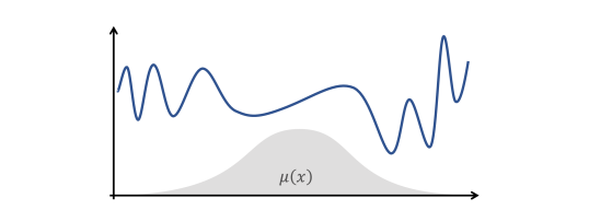
Figure 1: Illustration of a function and a measure $\mu$ exhibiting a large gap between “worst-case” smoothness (occurring in low density regions) and average-smoothness with respect to $\mu$.

Moreover, classically studied classes of average smoothness (e.g. Besov space) typically fix some distribution in advance (predominantly uniform), and then turn to consider smooth functions with respect to that single distribution. Thus, from a distribution-free statistical learning perspective — where the underlying distribution is assumed to be unknown — such classes fall short.

Seeking to address these drawbacks, Ashlagi et al. (2021) proposed a natural notion of average Lipschitz smoothness with respect to a distribution. Their average Lipschitz modulus can be considerably (even infinitely) smaller than the standard Lipschitz constant, while still being able to control the excess risk. However, the risk bounds obtained by Ashlagi et al. are far from optimal, while the optimal rates for distribution-free learning of average smoothness classes remained unknown. In particular, the cost of adapting to the smoothness with respect to the underlying distribution (in contrast to using classic worst-case smoothness) remained unclear so far.

Our contributions.

In this work, we generalize the aforementioned notion of average Lipschitz smoothness by extending it to Hölder smoothness of any exponent $\beta\in(0,1]$. After formally defining the average Hölder smoothness of a function with respect to a distribution in Section 2.1, our contributions can be summarized as follows:

• Bracketing numbers upper bound (Theorem 1). We establish a nearly-optimal distribution-free bound on the bracketing entropy of our proposed average-smooth function class, serving as the main crux on which we base our analyses throughout the paper. In particular, although it is known that asymptotically empirical covering numbers yield sharper bounds than bracketing numbers, in the case of average smoothness we reveal that the latter are tight up to a logarithmic factor.

• Realizable sample complexity (Theorem 2). We derive a nearly-optimal sample complexity required for uniform convergence of average-Hölder functions in the realizable case, which was not previously known even in the special case of average Lipschitz functions.

• Optimal realizable learning algorithm (Theorem 3). Since our notion of average smoothness is defined with respect to the unknown sampling distribution, the learner does not have an explicit representation of the function class, and hence is unable to execute ERM. We are able to overcome this obstacle by constructing a realizable nonparametric regression algorithm with a nearly-optimal learning rate. Such a rate was not previously known even in the special case of average Lipschitz smoothness.

• Agnostic learning algorithm (Theorem 4). We provide yet another learning algorithm for the fully agnostic (i.e. noisy) regression setting. Once again, our derived rate was not previously known even in the special case of average Lipschitz smoothness.

• Matching lower bound (Theorem 5). We prove a lower bound, showing that all the results mentioned above are tight up to logarithmic factors in the realizable case, establishing the (nearly) minimax risk rate for average-smooth classes.

• Illustrative comparisons (Section 7). Finally, we illustrate the extent to which the proposed smoothness notion is sharper than previously studied notions. We provide examples in which the “optimistic” average-Hölder constant is infinitely apart from both its “pessimistic” worst-case counterpart, or even the average-Lipschitz ($\beta=1$) constant, exemplifying the substantial (possibly infinite) speed-ups in terms of learning rates.

1.1 Related work.

The sample complexities associated to distribution-free learning of (classic) Hölder classes is well covered in the literature, see for example the books by Györfi et al. (2002); Tsybakov (2008).

Previous notions of average smoothness include Bounded Variation (BV) (Appell et al., 2014) in dimensions one and higher (Kuipers and Niederreiter, 1974; Niederreiter and Talay, 2006). One-dimensional BV has found learning-theoretic applications (Bartlett et al., 1997; Long, 2004; Anthony and Bartlett, 1999), but to our knowledge the higher-dimensional variants have not. Moreover, the positive results require $\mu$ to be uniformly distributed on a segment, and the aforementioned results break down for more general measures — especially if $\mu$ is not known to the learner.

Sobolev spaces, and the Sobolev-Slobodetskii norm in particular (Agranovich, 2015), bear some resemblance to our average Hölder smoothness. However, Ashlagi et al. (2021, Appendix I) demonstrate that from a learning-theoretic perspective this notion is inadequate for general (i.e., non-uniform or Lebesgue) measures, as it cannot be used to control sample complexity. Results for controlling bracketing in terms of various measures of average smoothness include Nickl and Pötscher (2007), who bound the bracketing numbers of Besov- and Sobolev-type classes and Malykhin (2010), who used the averaged modulus of continuity developed by Sendov and Popov (1988); again, these are all defined under the Lebesgue measure. While it is easy to define these smoothness notions with respect to arbitrary distributions, we are not aware of any existing work to bound their corresponding sample complexity (or even their covering or bracketing numbers) in a distribution-independent manner. Moreover, the smoothness notion studied in this paper is defined over arbitrary metric spaces, whereas previous notions are typically restricted to Euclidean structures (or variants thereof). Despite of the considerable generality of our setting, we are able to provide tight bounds for all metric spaces alike, without requiring specialized analyses.

A seminal work on recovering functions with spatially inhomogeneous smoothness from noisy samples is Donoho and Johnstone (1998). Arguably in the spirit of $\mu$-dependent Hölder smoothness, some of the classic results on $k$-NN risk decay rates were refined by Chaudhuri and Dasgupta (2014) via an analysis that captures the interplay between the metric and the sampling distribution. Another related notion is that of Probabilistic Lipschitzness (PL) (Urner and Ben-David, 2013; Urner et al., 2013; Kpotufe et al., 2015), which seeks to relax a hard Lipschitz condition on the regression function. While PL is in the same spirit as our notion, one critical distinction from our work is that, while existing analyses of learning under PL have focused specifically on binary classification, our interest in the present work is learning real-valued functions.

As previously mentioned, the main feature setting this work apart from others studying regression under average smoothness is that our notion is defined with respect to a general, unknown measure $\mu$. The notable exception is, of course, Ashlagi et al. (2021) — who introduced the framework of efficiently learning smooth-on-average functions with respect to an unknown distribution. Although extending their definition from Lipschitz to Hölder average smoothness was straightforward, optimal minimax rates are likely inaccessible via their techniques, which relied on empirical covering numbers. Estimating the magnitude of these random objects was a formidable challenge, and Ashlagi et al. were only able to do so to within an additive error decaying with sample size; this sampling noise appears to present an inherent obstruction to optimal rates. Thus, our results required a novel technique to overcome this obstruction, which we did by tightly controlling the bracketing entropy. Our Hölder-type extension is a direct adaptation of the Pointwise Minimum Slope Extension (PMSE) developed for the Lipschitz special case by Ashlagi et al., which in turn is closely related to the one introduced by Oberman (2008).

2 Preliminaries.

Setting.

Throughout the paper we consider functions $f:\Omega\to[0,1]$ where $(\Omega,\rho)$ is a metric space. We will consider a distribution $\mathcal{D}$ over $\Omega\times[0,1]$ with marginal $\mu$ over $\Omega$, such that $(\Omega,\rho,\mu)$ forms a metric probability space (namely, $\mu$ is supported on the Borel $\sigma$-algebra induced by $\rho$). We associate to any measurable function $f:\Omega\to[0,1]$ its $L_{1}$ risk $L_{\mathcal{D}}(f):=\mathop{\mathbb{E}}_{(X,Y)\sim\mathcal{D}}|f(X)-Y|$, and its empirical risk $L_{S}(f):=\frac{1}{n}\sum_{i=1}^{n}|f(X_{i})-Y_{i}|$ with respect to a sample $S=(X_{i},Y_{i})_{i=1}^{n}\sim\mathcal{D}^{n}$. More generally, we associate to any measurable function its $L_{1}$ norm $\|f\|_{L_{1}(\mu)}:=\mathop{\mathbb{E}}_{X\sim\mu}|f(X)|$, and given a sample $(X_{1},\dots,X_{n})\sim\mu^{n}$ we denote its $L_{1}$ norm with respect to the empirical measure $\|f\|_{L_{1}(\mu_{n})}:=\frac{1}{n}\sum_{i=1}^{n}|f(X_{i})|$.

We say that a distribution $\mathcal{D}$ over $\Omega\times[0,1]$ is realizable by a function class $\mathcal{F}\subset[0,1]^{\Omega}$ if there exists an $f^{*}\in\mathcal{F}$ such that $L_{\mathcal{D}}(f^{*})=0$. Thus, $f^{*}(X)=Y$ almost surely, where $(X,Y)\sim\mathcal{D}$.

Metric notions.

The diameter of $A\subset\Omega$ is $\mathrm{diam}(A):=\sup_{x,x^{\prime}\in A}\rho(x,x^{\prime})$, and we denote by $B(x,r):=\{x^{\prime}\in\Omega:\rho(x,x^{\prime})\leq r\}$ the closed ball around $x\in\Omega$ of radius $r>0$. For $t>0,~{}A,B\subset\Omega$, we say that $A$ is a $t$-cover of $B$ if $B\subset\bigcup_{a\in A}B(a,t)$, and define the $t$-covering number $\mathcal{N}_{B}(t)$ to be the minimal cardinality of any $t$-cover of $B$. We say that $A\subset B\subset\Omega$ is a $t$-packing of $B$ if $\rho(a,a^{\prime})\geq t$ for all $a\neq a^{\prime}\in A$. We call $V$ a $t$-net of $B$ if it is a $t$-cover and a $t$-packing. The induced Voronoi partition of $B$ with respect to a net $V$ is its partitioning into subsets sharing the same nearest neighbor in $V$ (with ties broken in some consistent arbitrary manner). A metric space $(\Omega,\rho)$ is said to be doubling if there exists $d\in\mathbb{N}$ such that every $r$-ball in $\Omega$ is contained in the union of some $d$ $r/2$-balls. The doubling dimension is defined as $\min_{d\geq 1}\log_{2}d$ where the minimum is taken over $d$ satisfying the doubling property.

Bracketing.

Given any two functions $l,u:\Omega\to[0,1]$, we say that $f:\Omega\to[0,1]$ belongs to the bracket $[l,u]$ if $l\leq f\leq u$. A set of brackets $\mathcal{B}$ is said to cover a function class $\mathcal{F}$ if any function in $\mathcal{F}$ belongs to some bracket in $\mathcal{B}$. We say that $[l,u]$ is a $t$-bracket with respect to a norm $\|\cdot\|$ if $\|u-l\|\leq t$. The $t$-bracketing number $\mathcal{N}_{[\,]}(\mathcal{F},\|\cdot\|,t)$ is defined as the minimal cardinality of any set of $t$-brackets that covers $\mathcal{F}$. The logarithm of this quantity is called the bracketing entropy.

Remark 1 (Covering vs. bracketing).

Having recalled two notions that quantify the “size” of a normed function space $(\mathcal{F},\|\cdot\|)$ — namely, its covering and bracketing numbers — it is useful to note they are related through

$$\mathcal{N}_{\mathcal{F}}(\varepsilon)\leq\mathcal{N}_{[\,]}(\mathcal{F},\|\cdot\|,2\varepsilon)~{},$$ (1)

though no converse inequality of this sort holds in general. On the other hand, the main advantage of using bracketing numbers for generalization bounds is that it suffices to bound the ambient bracketing numbers with respect to the distribution-specific metric, as opposed to the empirical covering numbers which are necessary to guarantee generalization (van der Vaart and Wellner, 1996, Section 2.1.1).

Strong and weak mean.

For any non-negative random variable $Z$ we define its weak mean by $\mathbb{W}[Z]:=\sup_{t>0}t\Pr[Z\geq t]$, and note that $\mathbb{W}[Z]\leq\mathop{\mathbb{E}}[Z]$ by Markov’s inequality. In the special case where $Z$ has finite support of size $N\geq 3$ where each atom has mass $1/N$ we have the reverse inequality $\mathop{\mathbb{E}}[Z]\leq 2\log(N)\mathbb{W}[Z]$ (Ashlagi et al., 2021, Lemma 22).

2.1 Average smoothness.

For $\beta\in(0,1]$ and $f:\Omega\to\mathbb{R}$, we define its $\beta$-slope at $x\in\Omega$ to be $\Lambda_{f}^{\beta}(x):=\sup_{y\in\Omega\setminus\{x\}}\frac{|f(x)-f(y)|}{\rho(x,y)^{\beta}}$. Recall that $f$ is called $\beta$-Hölder continuous if $\|f\|_{\mathrm{H\ddot{o}l}^{\beta}}:=\sup_{x\in\Omega}\Lambda_{f}^{\beta}(x)<\infty$, with this quantity serving as its Hölder seminorm. In particular, when $\beta=1$ these are exactly the Lipschitz functions equipped with the Lipschitz seminorm. For a metric probability space $(\Omega,\rho,\mu)$, we consider the average $\beta$-slope to be the mean of $\Lambda_{f}^{\beta}(X)$ where $X\sim\mu$. Namely, we define

$$\overline{\Lambda}_{f}^{\beta}(\mu) :=\mathbb{E}_{X\sim\mu}[\Lambda_{f}^{\beta}(X)]~{},$$

$$\widetilde{\Lambda}_{f}^{\beta}(\mu) :=\mathbb{W}_{X\sim\mu}[\Lambda_{f}^{\beta}(X)]=\sup_{t>0}\,t\cdot\mu(x:\Lambda_{f}^{\beta}(x)\geq t)~{}.$$

Notably,

$$\widetilde{\Lambda}_{f}^{\beta}(\mu)\leq\overline{\Lambda}_{f}^{\beta}(\mu)\leq\|f\|_{\mathrm{H\ddot{o}l}^{\beta}}~{},$$ (2)

where each subsequent pair can be infinitely apart — as we demonstrate in Section 7. Having defined notions of averaged smoothness, we can further define their corresponding function spaces

$$\mathrm{H\ddot{o}l}^{\beta}_{L}(\Omega) :=\left\{f:\Omega\to[0,1]\,:\,\|f\|_{\mathrm{H\ddot{o}l}^{\beta}}\leq L\right\},$$

$$\overline{\mathrm{H\ddot{o}l}}^{\beta}_{L}(\Omega,\mu) :=\left\{f:\Omega\to[0,1]\,:\,\overline{\Lambda}_{f}^{\beta}(\mu)\leq L\right\},$$

$$\widetilde{\mathrm{H\ddot{o}l}}^{\beta}_{L}(\Omega,\mu) :=\left\{f:\Omega\to[0,1]\,:\,\widetilde{\Lambda}_{f}^{\beta}(\mu)\leq L\right\}.$$

We occasionally omit $\mu$ when it is clear from context. Note that $\mathrm{H\ddot{o}l}^{\beta}_{L}(\Omega)\subset\overline{\mathrm{H\ddot{o}l}}^{\beta}_{L}(\Omega,\mu)\subset\widetilde{\mathrm{H\ddot{o}l}}^{\beta}_{L}(\Omega,\mu)$ due to Eq. (2), where both containments are strict in general. The special case of $\beta=1$ recovers the average-Lipschitz spaces $\mathrm{Lip}_{L}(\Omega)\subset\overline{\mathrm{Lip}}_{L}(\Omega,\mu)\subset\widetilde{\mathrm{Lip}}_{L}(\Omega,\mu)$ studied by Ashlagi et al. (2021).

3 Generalization bounds

Our first goal is to bound the bracketing entropy (namely, the logarithm of the bracketing number) of average-Hölder classes. We present this bound in full generality in terms of the underlying metric space, as captured by its covering number (see Corollary 1 for the typical scaling of covering numbers). As we will soon establish, this bound implies nearly-tight generalization guarantees in terms of the average smoothness constant.

Theorem 1.

For any metric probability space $(\Omega,\rho,\mu)$, any $\beta\in(0,1]$ and any $0<\epsilon<L$, it holds

$$\log\mathcal{N}_{[\,]}(\overline{\mathrm{H\ddot{o}l}}^{\beta}_{L}(\Omega,\mu),L_{1}(\mu),\varepsilon) \leq\log\mathcal{N}_{[\,]}(\widetilde{\mathrm{H\ddot{o}l}}^{\beta}_{L}(\Omega,\mu),L_{1}(\mu),\varepsilon)$$

$$\leq\mathcal{N}_{\Omega}\left(\left(\frac{\varepsilon}{128L\log(1/\varepsilon)}\right)^{1/\beta}\right)\cdot\log\left(\frac{16\log_{2}(1/\varepsilon)}{\varepsilon}\right)~{}.$$

Crucially, the bound above does not depend on $\mu$, allowing us to obtain distribution-free generalization guarantees. We defer the proof of Theorem 1 to Appendix 8.1. We start by showing that bounding the bracketing entropy implies a generalization bound in the realizable case:

Proposition 1.

Suppose $(\Omega,\rho)$ is a metric space, $\mathcal{F}\subseteq[0,1]^{\Omega}$ is a function class, and let $\mathcal{D}$ be a distribution over $\Omega\times[0,1]$ which is realizable by $\mathcal{F}$, with marginal $\mu$ over $\Omega$. Then with probability at least $1-\delta$ over drawing a sample $S\sim\mathcal{D}^{n}$ it holds that for all $f\in\mathcal{F}:$

$$L_{\mathcal{D}}(f)\leq 1.01L_{S}(f)+\inf_{\alpha\geq 0}\left(\alpha+\frac{205\log\mathcal{N}_{[\,]}(\mathcal{F},L_{1}(\mu),\alpha)}{n}\right)+\frac{205\log(1/\delta)}{n}~{}.$$

Remark 2 (Constant is arbitrary).

In Proposition 1 and in what follows, the constant multiplying $L_{S}(f)$ is arbitrary, and can be replaced by $(1+\gamma)$ for any $\gamma>0$ at the expense of multiplying the remaining summands by $\gamma^{-1}$. In the next section we will provide a realizable regression algorithm that returns an approximate empirical risk minimizer $f$ for which $L_{S}(f)\approx 0$, thus this constant will not matter for our purposes.

We prove Proposition 1 in Appendix 8.2. By combining Theorem 1 with Proposition 1 and setting $\alpha=\varepsilon/2$, we obtain the following realizable sample complexity result.

Theorem 2.

For any metric space $(\Omega,\rho)$, any $\beta\in(0,1]$ and any $0<\epsilon<L$, let $\mathcal{D}$ be a distribution over $\Omega\times[0,1]$ realizable by $\widetilde{\mathrm{H\ddot{o}l}}^{\beta}_{L}(\Omega,\mu)$. Then there exists $N=N(\beta,\varepsilon,\delta)\in\mathbb{N}$ satisfying

$$N=\widetilde{O}\left(\frac{\mathcal{N}_{\Omega}\left(\left(\frac{\varepsilon}{256L\log(1/\varepsilon)}\right)^{1/\beta}\right)+\log(1/\delta)}{\varepsilon}\right)$$

such that as long as $n\geq N$, with probability at least $1-\delta$ over drawing a sample $S\sim\mathcal{D}^{n}$ it holds that for all $f\in\widetilde{\mathrm{H\ddot{o}l}}^{\beta}_{L}(\Omega,\mu):$

$$L_{\mathcal{D}}(f)\leq 1.01L_{S}(f)+\varepsilon~{}.$$

The same claim holds for the smaller class $\overline{\mathrm{H\ddot{o}l}}^{\beta}_{L}(\Omega,\mu)$.

Corollary 1 (Doubling metrics).

In most cases of interest, $(\Omega,\rho)$ is a doubling metric space of some dimension $d$, e.g. when $\Omega$ is a subset of $\mathbb{R}^{d}$ (or more generally a $d$-dimensional Banach space). For $d$-dimensional doubling spaces of finite diameter we have $\mathcal{N}_{\Omega}(\varepsilon)\lesssim\left(\frac{1}{\varepsilon}\right)^{d}$ (Gottlieb et al., 2016, Lemma 2.1), which, plugged into Theorem 2, yields the simplified sample complexity bound

$$N=\widetilde{O}\left(\frac{L^{d/\beta}}{\varepsilon^{(d+\beta)/\beta}}\right)~{},$$

or equivalently

$$L_{\mathcal{D}}(f)\leq 1.01L_{S}(f)+\widetilde{O}\left(\frac{L^{d/(d+\beta)}}{n^{\beta/(d+\beta)}}\right)~{},$$

up to a constant which depends (exponentially) on $d$, but is independent of $L,n$.

Remark 3 (Tightness).

The bounds in Theorem 1 and Theorem 2 are both tight up to logarithmic factors, as we will prove in Section 6.

4 Realizable learning algorithm

Recall that without knowing $\mu$, the underlying distribution over $\Omega$, we cannot know for sure whether a function $f$ belongs to $\overline{\mathrm{H\ddot{o}l}}_{L}^{\beta}(\Omega,\mu)$ (except for the trivial case $f\in\mathrm{H\ddot{o}l}^{\beta}_{L}(\Omega)$). This gives rise to the challenge of designing a fully empirical algorithm — since standard empirical risk minimization is not possible. To that end, we provide the following algorithmic result with optimal guarantees (up to logarithmic factors).

Theorem 3.

For any metric space $(\Omega,\rho)$, any $\beta\in(0,1]$ and any $0<\epsilon<L$, let $\mathcal{D}$ be a distribution over $\Omega\times[0,1]$ realizable by $\overline{\mathrm{H\ddot{o}l}}^{\beta}_{L}(\Omega,\mu)$. Then there exists a polynomial time learning algorithm $\mathcal{A}$, which, given a sample $S\sim\mathcal{D}^{n}$ of size $n\geq N$ for some $N=N(\beta,\varepsilon,\delta)\in\mathbb{N}$ satisfying

$$N=\widetilde{O}\left(\frac{\mathcal{N}_{\Omega}\left(\left(\frac{\varepsilon}{256L\log(1/\varepsilon)}\right)^{1/\beta}\right)+\log(1/\delta)}{\varepsilon}\right),$$

constructs a hypothesis $f=\mathcal{A}(S)$ such that $L_{\mathcal{D}}(f)\leq\varepsilon$ with probability at least $1-\delta$.

Remark 4 (Doubling metrics).

As mentioned in Corollary 1, in most cases of interest we have $\mathcal{N}_{\Omega}(\varepsilon)\lesssim\left(\frac{1}{\varepsilon}\right)^{d}$. In that case, the algorithm above has sample complexity

$$N=\widetilde{O}\left(\frac{L^{d/\beta}}{\varepsilon^{(d+\beta)/\beta}}\right)~{},$$

or equivalently

$$L_{\mathcal{D}}(f)=\widetilde{O}\left(\frac{L^{d/(d+\beta)}}{n^{\beta/(d+\beta)}}\right)~{},$$

up to a constant which depends (exponentially) on $d$, but is independent of $L,n$.

Remark 5 (Computational complexity).

The algorithm constructed in Theorem 3 involves a one-time preprocessing step after which $f(x)$ can be evaluated at any given $x\in\Omega$ in $O(n^{2})$ time. We note that the computation at inference time matches that of (classic) Lipschitz/Hölder regression (e.g. Gottlieb et al., 2017). Furthermore, the computational complexity of the preprocessing step is similar to that in Ashlagi et al. (2021, Theorem 7) for the average Lipschitz case, where it is shown to run in time $\widetilde{O}(n^{2})$. The complexity analysis of our prepossessing step is entirely analogous to theirs, and we forgo repeating it here.

We will now outline the proof of Theorem 3, which appears in Section 8.3. The key idea is to analyze a natural fully-empirical quantity that will serve as an estimator of the true unknown average smoothness. To that end, given a sample $S=(X_{i},Y_{i})_{i=1}^{n}\sim\mathcal{D}^{n}$ and a function $f:\Omega\to[0,1]$, consider the following quantity which can be established directly from the data:

$$\widehat{\Lambda}^{\beta}_{f}:=\frac{1}{n}\sum_{i=1}^{n}\sup_{X_{j}\neq X_{i}}\frac{|f(X_{i})-f(X_{j})|}{\rho(X_{i},X_{j})^{\beta}}~{}.$$

Namely, this is the empirical average smoothness with respect to the sampled points. It would suit us well if the empirical average smoothness of a function did not greatly exceed its true average smoothness, with high probability. The fact something like this turns out to be true is somewhat surprising and may be of independent interest:

Proposition 2.

(Informal) Let $f^{*}:\Omega\to[0,1]$. Then with high probability $\widehat{\Lambda}_{f^{*}}^{\beta}\lesssim\overline{\Lambda}_{f^{*}}^{\beta}$ .

The proposition above implies that restricting to the sample, and letting $\widehat{f}(X_{i}):=Y_{i}$ yields a function over $\{X_{1},\dots,X_{n}\}$ which is empirically average-smooth over the sample (with high probability). We then turn to show that any such function can be approximately extended to the whole space, in a way that guarantees its average smoothness with respect to the underlying distribution.

Proposition 3.

(Informal) Let $\widehat{f}:\{X_{1},\dots,X_{n}\}\to[0,1]$ where $(X_{i})_{i=1}^{n}\sim\mu^{n}$. Then it is possible to construct $f:\Omega\to[0,1]$ such that with high probability $f(X_{i})\approx\widehat{f}(X_{i})$ for all $i\in[N]$, and $\overline{\Lambda}^{\beta}_{f}(\mu)\lesssim\widehat{\Lambda}^{\beta}_{\widehat{f}}$ .

We will now sketch the procedure described in Proposition 3, which serves as the main challenge in proving Theorem 3. Roughly speaking, the algorithm sorts the sampled points with respect to their relative slope to one another. Then, it discards a fraction of the sampled points with largest relative slope, which can be thought of as “outliers”. Then, the algorithm proceeds to extend the function in a smooth fashion among the remaining “well-behaved” samples. A careful probabilistic analysis shows that disregarding just the right amount of samples induces small error, while being average-smooth with high probability.

Overall this procedure yields a function $f:\Omega\to[0,1]$ which is an approximate empirical-minimizer (since $f(X_{i})\approx\widehat{f}(X_{i})=Y_{i}$), while guaranteed to be averagely-smooth with respect to the unknown distribution. Thus we can apply the uniform convergence of Theorem 2, proving Theorem 3.

5 Agnostic learning algorithm

Noticeably, up to this point, both the uniform convergence result we derived (Theorem 2) as well as the algorithmic result (Theorem 3) are tailored for the realizable regression setting. Inspired by a recent result of Hopkins et al. (2022) that showed a reduction from agnostic learning to realizable learning, we provide an algorithm for agnostic (i.e. noisy) regression of average-smooth functions. It is worth noting that the following algorithm does not require any prior assumption on the noise model, unlike many nonparametric regression methods, due to our distribution free analysis.

Theorem 4.

There exists a learning algorithm $\mathcal{A}$ such that for any metric space $(\Omega,\rho)$, any $\beta\in(0,1],~{}0<\epsilon<L$, and any distribution $\mathcal{D}$ over $\Omega\times[0,1]$, given a sample $S\sim\mathcal{D}^{n}$ of size $n\geq N$ for some $N=N(\beta,\varepsilon,\delta)$ satisfying

$$N=\widetilde{O}\left(\frac{\mathcal{N}_{\Omega}\left(\left(\frac{\varepsilon}{640L\log(1/\varepsilon)}\right)^{1/\beta}\right)+\log(1/\delta)}{\varepsilon^{2}}\right),$$

the algorithm constructs a hypothesis $f=\mathcal{A}(S)$ such that $L_{\mathcal{D}}(f)\leq\inf_{f^{*}\in\overline{\mathrm{H\ddot{o}l}}_{L}^{\beta}(\Omega,\mu)}L_{\mathcal{D}}(f^{*})+\epsilon$ with probability at least $1-\delta$.

Remark 6 (Doubling metrics).

As mentioned in Corollary 1, in most cases of interest we have $\mathcal{N}_{\Omega}(\varepsilon)\lesssim\left(\frac{1}{\varepsilon}\right)^{d}$. In that case, the algorithm above has sample complexity

$$N=\widetilde{O}\left(\frac{L^{d/\beta}}{\varepsilon^{(d+2\beta)/\beta}}\right)~{},$$

or equivalently

$$L_{\mathcal{D}}(f)=\inf_{f^{*}\in\overline{\mathrm{H\ddot{o}l}}_{L}^{\beta}(\Omega,\mu)}L_{\mathcal{D}}(f^{*})+\widetilde{O}\left(\frac{L^{d/(d+2\beta)}}{n^{\beta/(d+2\beta)}}\right)~{},$$

up to a constant which depends (exponentially) on $d$, but is independent of $L,n$.

Though our agnostic algorithm is similar in spirit to that obtained by the reduction of Hopkins et al. (2022), our analysis is self-contained and crucially relies on the bracketing bound given by Theorem 1, as well as analyzing the empirical smoothness estimator as provided by Proposition 2. We also note that unlike our algorithm for realizable learning, the agnostic algorithm is not computationally efficient. This seems to be inherent for such reductions, and we do not know whether this blow-up in running time can be avoided or not.

We will now describe the proof of Theorem 4 which appears in Section 8.4. Given a sample $S$ of size $n$, consider dividing it into two sub-samples $S_{1}\cup S_{2}=S$ of size $n/2$ each. We first use $S_{1}$ in order to construct an empirical $\epsilon$-net $h_{1},\dots,h_{N}:S_{1}\to[0,1]$, namely a set of functions which are sufficiently empirically smooth over the sample, yet far away enough from one another when averaged over the sample. Recalling that bracketing numbers upper bound covering numbers (Eq. (1)), and since Theorem 1 holds true for every measure (in particular for the empirical measure), we can bound $\log N\lesssim\mathcal{N}_{\Omega}((\epsilon/L)^{1/\beta})$. Moreover, using Proposition 2 we know that $f^{*}:=\arg\min_{f\in\overline{\mathrm{H\ddot{o}l}}_{L}^{\beta}(\Omega,\mu)}L_{\mathcal{D}}(f)$ is likely to be $\widetilde{O}(L)$ average-smooth over $S_{1}$, so there must exist some $h_{j}$ with $\epsilon$ excess empirical loss (since $f^{*}$ is in the class we are $\epsilon$-covering). Thus running the realizable algorithm of Theorem 3 over all $\{h_{1},\dots,h_{N}\}$, producing $f_{1},\dots,f_{N}:\Omega\to[0,1]$, yields at least one function which has both small excess empirical error, while being smooth with respect to the underlying distribution. Finally, running ERM over $\{f_{1},\dots,f_{N}\}$ with respect to the fresh sample $S_{2}$ reveals such a good candidate function within $\frac{\log(N)+\log(1/\delta)}{\epsilon^{2}}$ samples by applying standard uniform convergence for finite classes (i.e. Hoeffding’s inequality with the union bound).

6 Lower bound

We now turn to show that the bounds proved in Theorem 1, Theorem 2 and Theorem 3 are all tight up to logarithmic factors. In fact, since the bracketing entropy bound of Theorem 1 implies the generalization bound of Theorem 2 and the latter implies the sample complexity in Theorem 3, it is enough to show that the latter is nearly optimal.

Theorem 5.

For any $\beta\in(0,1],~{}\varepsilon\in(0,1)$ any metric space $(\Omega,\rho)$ and $L\geq\frac{8}{\mathrm{diam}(\Omega)}$, there exists a distribution $\mathcal{D}$ over $\Omega\times[0,1]$ which is realizable by $\overline{\mathrm{H\ddot{o}l}}^{\beta}_{L}(\Omega)$ such that any learning algorithm that produces $f=A(S)$ with $L_{\mathcal{D}}(f)\leq\varepsilon$ with constant probability, must have sample complexity

$$n=\Omega\left(\frac{\mathcal{N}_{\Omega}((\varepsilon/L)^{1/\beta})}{\varepsilon}\right)~{}.$$

Remark 7 (Typical case).

In most cases of interest it holds that $\mathcal{N}_{\Omega}(\varepsilon)\gtrsim\left(\frac{1}{\varepsilon}\right)^{d}$ for some constant $d$, e.g. when $\Omega$ is a subset of non-empty interior in $\mathbb{R}^{d}$ (or more generally in any $d$-dimensional Banach space). That being the case, Theorem 5 yields the simplified sample complexity lower bound of

$$n=\Omega\left(\frac{L^{d/\beta}}{\varepsilon^{(d+\beta)/\beta}}\right)$$

Equivalently, we obtain an excess risk lower bound of

$$L_{\mathcal{D}}(f)=\Omega\left(\frac{L^{d/(d+\beta)}}{n^{\beta/(d+\beta)}}\right)~{}.$$

We will now provide a proof sketch of Theorem 5, while the full proof appears in Section 8.5. Suppose $K\subset\Omega$ is a $(\varepsilon/L)^{1/\beta}$-net of most of $\Omega$, yet $x_{0}\in\Omega$ is some “isolated” point at constant distance away from $K$ (we show that such $x_{0},K$ always exist). Let $\mu$ be the measure that assigns $1-\varepsilon$ probability mass to $x_{0}$, while the rest of the probability mass is distributed uniformly over $K$. Now consider a (random) function that independently assigns either $0$ or $1$ to each point in $K$ uniformly, and is constant over $x_{0}$. Since points in $K$ are $(\varepsilon/L)^{1/\beta}$ away from one another, the local $\beta$-slope at each point in $K$ is roughly $1/((\varepsilon/L)^{1/\beta})^{\beta}=L/\varepsilon$, while the slope at $x_{0}$ is small since it is far enough from other points. Averaging over the space with respect to $\mu$, we see that the function is $\mu(K)\cdot L/\varepsilon=L$ average-Hölder. Now, we imitate the standard lower bound proof for VC classes over $K$: Since any point in $K$ is sampled with probability $\varepsilon/|K|$, any learning algorithm with much fewer than $|K|/\varepsilon\approx\mathcal{N}_{\Omega}((\varepsilon/L)^{1/\beta})/\varepsilon$ examples will guess wrong a large portion of $K$, suffering $L_{1}$-loss of at least order of $\mu(K)=\varepsilon$.

7 Illustrative examples

Having established the control that average-Hölder smoothness has on generalization, we illustrate the vast possible gap between the average smoothness and it’s “worst-case” classic counterpart. Indeed, in the examples we provide, the gap is infinite. Moreover, we also show that classes of average-Hölder smoothness are significantly richer than the previously studied average-Lipschitz, motivating the more general Hölder framework considered in this work. Finally, it is illuminating to notice that both claims to follow actually consist of the same simple function $f(x)=\boldsymbol{1}[x>\frac{1}{2}]$ though with respect to different distributions, emphasizing the crucial role of the underlying distribution in terms of establishing the function classes.

Claim 6.

For any $L>0,\beta\in(0,1)$, there exist $f:\Omega\to[0,1]$ and a probability measure $\mu$ such that

• $f$ is average-Hölder: $f\in\overline{\mathrm{H\ddot{o}l}}^{\beta}_{L}(\Omega,\mu)$ .

• $f$ is not Hölder with any finite Hölder constant: For all $M>0:~{}f\notin{\mathrm{H\ddot{o}l}}_{M}^{\beta}(\Omega)$ .

• $f$ is not (even) weakly-average-Lipschitz with any finite modulus: For all $M>0:f\notin\widetilde{\mathrm{Lip}}_{M}(\Omega,\mu)$ .

Thus, $\overline{\mathrm{H\ddot{o}l}}^{\beta}_{L}(\Omega,\mu)\not\subset\bigcup_{M=0}^{\infty}\left({\mathrm{H\ddot{o}l}}_{M}^{\beta}(\Omega)\cup\widetilde{\mathrm{Lip}}_{M}(\Omega,\mu)\right)$.

Claim 7.

For any $L>0,\beta\in(0,1)$, there exist $f:\Omega\to[0,1]$ and a probability measure $\mu$ such that

• $f$ is weakly-average-Hölder: $f\in\widetilde{\mathrm{H\ddot{o}l}}^{\beta}_{L}(\Omega,\mu)$ .

• $f$ is not strongly-average-Hölder with any finite modulus: For all $M>0:~{}f\notin\overline{\mathrm{H\ddot{o}l}}_{M}^{\beta}(\Omega)$ .

• $f$ is not (even) weakly-average-Lipschitz with any finite modulus: For all $M>0:f\notin\widetilde{\mathrm{Lip}}_{M}(\Omega,\mu)$ .

Thus, $\widetilde{\mathrm{H\ddot{o}l}}^{\beta}_{L}(\Omega,\mu)\not\subset\bigcup_{M=0}^{\infty}\left(\overline{\mathrm{H\ddot{o}l}}_{M}^{\beta}(\Omega,\mu)\cup\widetilde{\mathrm{Lip}}_{M}(\Omega,\mu)\right)$.

We prove both of the claims above in Section 8.6.

8 Proofs

8.1 Proof of Theorem 1

We start by stating a strengthened version of the triangle inequality (also known as the “snowflake” triangle inequality) which we will use later on. For any $\beta\in(0,1],~{}x\neq y,z\in\Omega$:

$$\rho(x,y)^{\beta}\leq\rho(x,z)^{\beta}+\rho(z,y)^{\beta}~{}.$$ (3)

Indeed, this follows from

$$\frac{\rho(x,z)^{\beta}+\rho(z,y)^{\beta}}{\rho(x,y)^{\beta}} \geq\frac{\rho(x,z)^{\beta}+\rho(z,y)^{\beta}}{(\rho(x,z)+\rho(z,y))^{\beta}}=\left(\frac{\rho(x,z)}{\rho(x,z)+\rho(z,y)}\right)^{\beta}+\left(\frac{\rho(z,y)}{\rho(x,z)+\rho(z,y)}\right)^{\beta}$$

$$\geq\left(\frac{\rho(x,z)}{\rho(x,z)+\rho(z,y)}\right)+\left(\frac{\rho(z,y)}{\rho(x,z)+\rho(z,y)}\right)=1~{}.$$

Let $0<\varepsilon<\frac{1}{4}$, denote $K:=\lceil\log_{2}(1/\varepsilon)\rceil,~{}\varepsilon^{\prime}:=\frac{1}{(K+1)2^{K}}$ and note that

$$\varepsilon^{\prime}\geq\frac{1}{\left(\log_{2}(1/\varepsilon)+2\right)2^{\log_{2}(1/\varepsilon)+1}}=\frac{\varepsilon}{2\left(\log_{2}(1/\varepsilon)+2\right)}\geq\frac{\varepsilon}{4\log_{2}(1/\varepsilon)}~{}.$$ (4)

Let $N=\{x_{1},\dots,x_{|N|}\}$ be a $\left(\frac{\varepsilon^{\prime}}{32L}\right)^{1/\beta}$-net of $\Omega$ of size $|N|=\mathcal{N}_{\Omega}\left(\left(\frac{\varepsilon^{\prime}}{32L}\right)^{1/\beta}\right)$, and let $\Pi=\{C_{1},\dots,C_{|N|}\}$ be its induced Voronoi partition. We define $\mathcal{B}=\{[l_{j},u_{j}]\}_{j\in J}\subset[0,1]^{\Omega}\times[0,1]^{\Omega}$ to be the pairs of functions constructed as follows:

• $l,u$ are both constant over every cell $C_{i}\in\Pi$, and map each cell to a value in $\{0,\frac{\varepsilon^{\prime}}{2},\varepsilon^{\prime},\frac{3\varepsilon^{\prime}}{2},\dots,1\}$.

• Choose some cells $S_{1}\subset\Pi$ such that $\mu(\bigcup_{C_{i}\in S_{1}}C_{i})\leq\varepsilon^{\prime}$ and set for any $C_{i}\in S_{1}:\ l|_{C_{i}}=0,~{}u|_{C_{i}}=1$.

• For $m=2,\dots,K$ choose some “unchosen” cells $S_{m}\subset\Pi\setminus\bigcup_{j<m}S_{j}$ such that $\mu(\bigcup_{C_{i}\in S_{m}}C_{i})\leq 2^{m-1}\varepsilon^{\prime}$ and set for any $C_{i}\in S_{m}:\ l|_{C_{i}}\in\{0,\frac{1}{2^{m}},\frac{2}{2^{m}},\dots,\frac{2^{m}-2}{2^{m}}\},~{},~{}u|_{C_{i}}=l+\frac{1}{2^{m-1}}$.

• In the ”remaining” cells $S_{K+1}:=\Pi\setminus\bigcup_{j\leq K}S_{j}$ set for any $C_{i}\in S_{K+1}:$

  $$l|_{C_{i}}\in\left\{0,\frac{1}{2^{K+1}},\frac{2}{2^{K+1}},\dots,\frac{2^{K+1}-2}{2^{K+1}}\right\},~{}u|_{C_{i}}=l+\frac{1}{2^{{K}}}~{}.$$

Notice that for any $[l,u]\in\mathcal{B}$ we have

$$\|l-u\|_{L^{1}(\mu)} =\sum_{C_{i}\in\Pi}\int_{C_{i}}|l(x)-u(x)|d\mu(x)=\sum_{m=1}^{K+1}\sum_{C_{i}\in S_{m}}\int_{C_{i}}|l(x)-u(x)|d\mu(x)$$

$$=\sum_{m=1}^{K+1}\sum_{C_{i}\in S_{m}}\int_{C_{i}}\frac{1}{2^{m-1}}d\mu(x)=\sum_{m=1}^{K+1}\frac{1}{2^{m-1}}\sum_{C_{i}\in S_{m}}\mu(C_{i})$$

$$=\sum_{m=1}^{K+1}\frac{2^{m-1}\varepsilon^{\prime}}{2^{m-1}}=\varepsilon^{\prime}(K+1)=\frac{1}{2^{K}}\leq\varepsilon~{}.$$

Furthermore, we can bound $|\mathcal{B}|$ by noticing that any such $l$ is defined by its values over $|N|$ cells who all belong to $\{0,\frac{\varepsilon^{\prime}}{2},\varepsilon^{\prime},\dots,1\}$, and that once $l$ is fixed then any associated $u$ has at most $K+1$ possible values over each cell since it equals $l+\frac{1}{2^{m-1}}$ for some $m\in[K+1]$. Thus

$$|\mathcal{B}|\leq(K+1)\left(\frac{8}{\varepsilon^{\prime}}\right)^{|N|}\leq\log_{2}\left(\frac{1}{\varepsilon}\right)\cdot\left(\frac{16\log_{2}(1/\varepsilon)}{\varepsilon}\right)^{\mathcal{N}\left(\left(\frac{\varepsilon}{128L\log(1/\varepsilon)}\right)^{1/\beta}\right)}~{},$$

where the last inequality uses Eq. (4) and definition of $K$. In order to finish the proof, in remains to show that $\mathcal{B}$ indeed cover $\widetilde{\mathrm{H\ddot{o}l}}_{L}^{\beta}(\Omega,\mu)$ as brackets. Namely, that for any $f\in\widetilde{\mathrm{H\ddot{o}l}}_{L}^{\beta}(\Omega,\mu)$ there exist $[l,u]\in\mathcal{B}$ such that $l\leq f\leq u$. To that end, let $f\in\widetilde{\mathrm{H\ddot{o}l}}_{L}^{\beta}(\Omega,\mu)$. Denote

$$S_{1}^{f}:=\left\{C_{i}\in\Pi\mathrm{~{}:~{}}\forall x\in C_{i}:\Lambda_{f}^{\beta}(x)\geq\frac{L}{\varepsilon^{\prime}}\right\}$$

and notice that $\bigcup\{C_{i}\in S_{1}^{f}\}\subseteq\{x:\Lambda_{f}^{\beta}(x)\geq L/\varepsilon^{\prime}\}\implies\mu(\bigcup\{C_{i}\in S_{1}^{f}\})\leq\varepsilon^{\prime}$. Hence we can pick $[l,u]\in\mathcal{B}$ such that $(l|_{C_{i}},u|_{C_{i}})\equiv(0,1)$ for any $C_{i}\in S^{f}_{1}$ (serving as $S_{1}$ in their construction). Clearly any such $l,u$ bound $f$ over these cells. Furthermore, for $m=2,\dots,K$ we denote

$$S_{m}^{f}:=\left\{C_{i}\in\Pi\setminus\bigcup_{j<m}S_{j}^{f}\mathrm{~{}:~{}}\forall x\in C_{i}:\Lambda_{f}^{\beta}(x)\geq\frac{L}{2^{m-1}\varepsilon^{\prime}}~{}\right\}~{},$$

and notice that $\bigcup\{C_{i}\in S_{m}^{f}\}\subseteq\{x:\Lambda_{f}^{\beta}(x)\geq L/(2^{m-1}\varepsilon^{\prime})\}\implies\mu(\bigcup\{C_{i}\in S_{m}^{f}\})\leq 2^{m-1}\varepsilon^{\prime}$. Consequently we can let $S^{f}_{m}$ serve as $S_{m}$ in the construction of $[l,u]\in\mathcal{B}$, assuming we will show such a choice can serve as a bracket of $f$ over such cells. Indeed, for any $x\in C_{i}$ we have

$$|f(x)-f(z_{i})|\leq\Lambda_{f}^{\beta}(z_{i})\cdot\rho(x,z_{i})^{\beta}\overset{Eq.~{}(\ref{eq: beta triangle ineq})}{\leq}\frac{L}{2^{m-2}\varepsilon^{\prime}}\cdot\frac{2\varepsilon^{\prime}}{32L}=\frac{1}{2^{m+2}},$$

which by the triangle inequality shows in particular that for any $x,y\in C_{i}:$

$$|f(x)-f(y)|\leq|f(x)-f(z_{i})|+|f(z_{i})-f(y)|\leq\frac{1}{2^{m+1}}=\frac{1}{4\cdot 2^{m-1}}~{}.$$

So clearly there exists $\alpha_{i}\in\{0,\frac{1}{2^{m}},\frac{2}{2^{m}},\dots,\frac{2^{m}-2}{2^{m}}\}$ such that $\alpha_{i}\leq f|_{C_{i}}\leq\alpha_{i}+\frac{1}{2^{m-1}}$, and by setting $l|_{C_{i}},u|_{C_{i}}=(\alpha_{i},\alpha_{i}+\frac{1}{2^{m-1}})$ for any $C_{i}\in S^{f}_{m}$ we ensure the bracketing property. Finally, for any of the remaining cells $S_{K+1}^{f}:=\Pi\setminus\bigcup_{j\leq K}S_{j}^{f}$ we get by construction that $\exists z_{i}\in C_{i}:\Lambda_{f}^{\beta}(z_{i})<\frac{L}{2^{K}\varepsilon^{\prime}}$ (otherwise they would satisfy the condition for some previously constructed $S_{m}^{f}$). Hence for any $x\in C_{i}$ we have

$$|f(x)-f(z_{i})|\leq\Lambda_{f}^{\beta}(z_{i})\cdot\rho(x,z_{i})^{\beta}\overset{Eq.~{}(\ref{eq: beta triangle ineq})}{\leq}\frac{L}{2^{K}\varepsilon^{\prime}}\cdot\frac{2\varepsilon^{\prime}}{32L}=\frac{1}{2^{K+4}},$$

which by the triangle inequality shows that for any $x,y\in C_{i}:$

$$|f(x)-f(y)|\leq\frac{1}{2^{K+3}}=\frac{1}{8\cdot 2^{K}}~{}.$$

So as before, there clearly exists $\alpha_{i}\in\{0,\frac{1}{2^{K+1}},\frac{2}{2^{K+1}},\dots,\frac{2^{K+1}-2}{2^{K+1}}\}$ such that $\alpha_{i}\leq f|_{C_{i}}\leq\alpha_{i}+\frac{1}{2^{K}}$, and by setting $l|_{C_{i}},u|_{C_{i}}=(\alpha_{i},\alpha_{i}+\frac{1}{2^{K}})$ for any $C_{i}\in S^{f}_{m}$ we ensure the bracketing property over all of $\Omega$, which finishes the proof.

8.2 Proof of Proposition 1

Recalling that the realizability assumption ensures a “perfect” predictor $f^{*}\in\mathcal{F}$, we start by introducing the loss class $\mathcal{L}_{\mathcal{F}}\subset[0,1]^{\Omega}:$

$$\mathcal{L}_{\mathcal{F}}=\{\ell_{f}(x):=|f(x)-f^{*}(x)|:f\in\mathcal{F}\}~{}.$$

Fix $\alpha>0$. We observe that $\mathcal{L}_{\mathcal{F}}$ is no larger than $\mathcal{F}$ in terms of bracketing entropy, namely

$$\mathcal{N}_{[\,]}(\mathcal{L}_{\mathcal{F}},L_{1}(\mu),\alpha)\leq\mathcal{N}_{[\,]}(\mathcal{F},L_{1}(\mu),\alpha)~{}.$$ (5)

Indeed, suppose we are given an $\alpha$-bracketing of $\mathcal{F}$ denoted by $\mathcal{B}_{\alpha}$, and denote for any $f\in\mathcal{F}$ by $[l_{f},u_{f}]\in\mathcal{B}_{\alpha}$ its associated bracket. Then any $\ell_{f}\in\mathcal{L}_{\mathcal{F}}$ is inside the bracket $[l_{\ell_{f}},u_{\ell_{f}}]$ where

$$l_{\ell_{f}}:= ~{}\max\{0\,,\,\min\{l_{f}-f^{*},f^{*}-u_{f}\}\}~{},$$

$$u_{\ell_{f}}:= ~{}\min\{1\,,\,\max\{u_{f}-f^{*},f^{*}-l_{f}\}\}~{}.$$

It is straightforward to verify that $\|u_{\ell_{f}}-l_{\ell_{f}}\|_{L_{1}(\mu)}\leq\|u_{f}-l_{f}\|_{L_{1}(\mu)}\leq\alpha$, and clearly the set of all such brackets is of size at most $|\mathcal{B}_{\alpha}|$, yielding Eq. (5).

Now notice that for any $f\in\mathcal{F}:$

$$L_{\mathcal{D}}(f)-1.01L_{S}(f)=\|\ell_{f}\|_{L_{1}(\mu)}-1.01\|\ell_{f}\|_{L_{1}(\mu_{n})}\leq\alpha+\|l_{\ell_{f}}\|_{L_{1}(\mu)}-1.01\|l_{\ell_{f}}\|_{L_{1}(\mu_{n})}~{},$$

hence

$$\sup_{f\in\mathcal{F}}\left(L_{\mathcal{D}}(f)-1.01L_{S}(f)\right)\leq\alpha+\max_{l_{\ell_{f}}}(\|l_{\ell_{f}}\|_{L_{1}(\mu)}-1.01\|l_{\ell_{f}}\|_{L_{1}(\mu_{n})})~{}.$$ (6)

In order to bound the right hand side, fix some $l_{\ell_{f}}$, and note that $\mathrm{Var}(l_{\ell_{f}})\leq\|l_{\ell_{f}}^{2}\|_{L_{1}(\mu)}\leq\|l_{\ell_{f}}\|_{L_{1}(\mu)}$, since $l_{\ell_{f}}(x)\in[0,1]$. Thus by Bernstein’s inequality and the AM-GM inequality we get that with probability at least $1-\gamma:$

$$\|l_{\ell_{f}}\|_{L_{1}(\mu)}-\|l_{\ell_{f}}\|_{L_{1}(\mu_{n})}\leq~{} \frac{\log(1/\gamma)}{n}+\sqrt{\frac{2\|l_{\ell_{f}}\|_{L_{1}(\mu)}\log(1/\gamma)}{n}}$$

$$\leq~{} \frac{202\log(1/\gamma)}{n}+\frac{1}{101}\|l_{\ell_{f}}\|_{L_{1}(\mu)}$$

$$\implies\|l_{\ell_{f}}\|_{L_{1}(\mu)}-1.01\|l_{\ell_{f}}\|_{L_{1}(\mu_{n})}\leq~{} \frac{205\log(1/\gamma)}{n}~{}.$$

Setting $\gamma=\delta/\mathcal{N}_{[\,]}(\mathcal{F},L_{1}(\mu),\alpha)$ and taking a union bound over $l_{\ell_{f}}$ whose number is bounded due to Eq. (5), we see that with probability $1-\delta:$

$$\max_{l_{\ell_{f}}}(\|l_{\ell_{f}}\|_{L_{1}(\mu)}-1.01\|l_{\ell_{f}}\|_{L_{1}(\mu_{n})})\leq\frac{205\log\mathcal{N}_{[\,]}(\mathcal{F},L_{1}(\mu),\alpha)+205\log(1/\delta)}{n}~{}.$$

Plugging this back into Eq. (6), and minimizing over $\alpha>0$ finishes the proof.

8.3 Proof of Theorem 3

Proposition 2.

Let $f:\Omega\to[0,1]$. Then with probability at least $1-\delta/2$ over drawing a sample it holds that

$$\widehat{\Lambda}_{f}^{\beta}\leq 4\log^{2}(4n/\delta)\overline{\Lambda}_{f}^{\beta}(\mu)+\frac{4\log^{2}(4n/\delta)}{n}~{}.$$

Corollary 2.

If $\mathcal{D}$ is realizable by $\overline{\mathrm{H\ddot{o}l}}^{\beta}_{L}(\Omega,\mu)$, then for $f^{*}:\Omega\to[0,1]$ such that $L_{\mathcal{D}}(f^{*})=0$ it holds with probability at least $1-\delta/2:~{}\widehat{\Lambda}^{\beta}_{f^{*}}\leq 5\log^{2}(4n/\delta)L$. Hence, $\widehat{f}(X_{i}):=f^{*}(X_{i})=Y_{i}$ satisfies $L_{S}(\widehat{f})=0$ and $\widehat{\Lambda}^{\beta}_{\widehat{f}}\leq 5\log^{2}(4n/\delta)L$ .

Proof.

(of Proposition 2) Fix $f:\Omega\to[0,1]$. Given a sample $(X_{i})_{i=1}^{n}\sim\mu^{n}$ which induces an empirical measure $\mu_{n}$, we get

$$\widehat{\Lambda}_{f}^{\beta}\leq\frac{1}{n}\sum_{i=1}^{n}\sup_{z\neq X_{i}}\frac{|f(X_{i})-f(z)|}{\rho(X_{i},z)^{\beta}}=\mathop{\mathbb{E}}_{X\sim\mu_{n}}[\Lambda_{f}^{\beta}(X)]\leq 2\log(n)\mathbb{W}_{X\sim\mu_{n}}[\Lambda_{f}^{\beta}(X)]~{},$$ (7)

where the last inequality follows from the reversed strong-weak mean inequality for uniform measures. We will now show that with high probability $\mathbb{W}_{X\sim\mu_{n}}[\Lambda_{f}^{\beta}(X)]\lesssim\mathbb{W}_{X\sim\mu}[\Lambda_{f}^{\beta}(X)]=\widetilde{\Lambda}_{f}^{\beta}$. To that end, we denote for any $t>0:\,M_{f}(t):=\{x:\Lambda_{f}^{\beta}(x)\geq t\}\subset\Omega$, let $K:=\widetilde{\Lambda}_{f}^{\beta}(\mu),~{}N:=\lceil 2\log(4n/\delta)\log\log(4n/\delta)\rceil$ and note that

$$\mathbb{W}_{X\sim\mu_{n}}[\Lambda_{f}^{\beta}(X)] =\sup_{t>0}t\mu_{n}(M_{f}(t))$$ (8)

$$\leq\sup_{0<t\leq K}t\mu_{n}(M_{f}(t))+2\max_{j\in\{0,1,\dots,N-1\}}2^{j}K\mu_{n}(M_{f}(2^{j}K))+\sup_{t\geq 2^{N}K}t\mu_{n}(M_{f}(t))~{}.$$

We will bound all three summands above. We easily bound the first term by

$$\sup_{0<t\leq K}t\mu_{n}(M_{f}(t))\leq K\cdot 1=\widetilde{\Lambda}_{f}^{\beta}(\mu)~{}.$$ (9)

For the second term, denote for any $t>0$ by $M_{f}^{+}(t)\supset M_{f}(t)$ a containing set for which $\frac{1}{n}\leq\mu(M_{f}^{+}(t))\leq\mu(M_{f}(t))+\frac{1}{n}$. We can always assume without loss of generality that such a set exists. By the multiplicative Chernoff bound we have for any $t,\alpha>0:$

$$\Pr_{S}\left[\mu_{n}(M_{f}^{+}(t))\geq(1+\alpha)\mu(M_{f}^{+}(t))\right]\leq\frac{e^{\alpha}}{(1+\alpha)^{1+\alpha}}~{},$$

hence by the union bound we get with probability at least $1-\frac{Ne^{\alpha}}{(1+\alpha)^{1+\alpha}}:$

$$\max_{j\in\{0,1,\dots,N-1\}}2^{j}K\mu_{n}(M_{f}(2^{j}K)) \leq\max_{j\in\{0,1,\dots,N-1\}}2^{j}K\mu_{n}(M_{f}^{+}(2^{j}K))$$

$$\leq(1+\alpha)\max_{j\in\{0,1,\dots,N-1\}}2^{j}L\mu(M_{f}^{+}(2^{j}K))$$

$$\leq(1+\alpha)\max_{j\in\{0,1,\dots,N-1\}}2^{j}K\left(\mu(M_{f}(2^{j}K))+\frac{1}{n}\right)$$

$$\leq(1+\alpha)\widetilde{\Lambda}^{\beta}_{f}(\mu)+\frac{1+\alpha}{n}~{}.$$

Letting $\alpha=\log(4n/\delta)-1$, by our choice of $N=\lceil 2\log(4n/\delta)\log\log(4n/\delta)\rceil$ we get that with probability at least $1-\delta/4:$

$$2\max_{j\in\{0,1,\dots,N-1\}}2^{j}K\mu_{n}(M_{f}(2^{j}K))\leq 2\log(4n/\delta)\widetilde{\Lambda}^{\beta}_{f}(\mu)+\frac{2\log(4n/\delta)}{n}~{}.$$ (10)

In order to bound the last term in Eq. (8), we observe that the empirical measure satisfies for any $A\subset\Omega:\mu_{n}(A)<\frac{1}{n}\iff\mu_{n}(A)=0$, and that $M_{f}(s)\subset M_{f}(t)$ for $s>t$. Furthermore, by definition of $K=\widetilde{\Lambda}_{f}^{\beta}(\mu)$ we have $\mu(M_{f}(t))\leq\frac{K}{t}$, hence by Markov’s inequality

$$\Pr_{S}\left[\sup_{s\geq t}\mu_{n}(M_{f}(s))\neq 0\right]\leq\Pr_{S}\left[\mu_{n}(M_{f}(t))\neq 0\right]=\Pr_{S}\left[\mu_{n}(M_{f}(t))\geq\frac{1}{n}\right]\leq\frac{nK}{t}~{}.$$

For $t:=2^{N}K$ yields $\Pr_{S}\left[\sup_{s\geq 2^{n}K}\mu_{n}(M_{f}(s))\neq 0\right]\leq\frac{n}{2^{N}}\leq\frac{\delta}{4}$. Combining this with Eq. (9), Eq. (10) and plugging back into Eq. (8), we get that with probability at least $1-\delta/2:$

$$\mathbb{W}_{X\sim\mu_{n}}[\Lambda^{\beta}_{f}(X)]\leq(1+2\log(4n/\delta))\widetilde{\Lambda}_{f}^{\beta}(\mu)+\frac{2\log(4n/\delta)}{n}\leq(1+2\log(4n/\delta))\overline{\Lambda}_{f}^{\beta}(\mu)+\frac{2\log(4n/\delta)}{n}~{}.$$

Recalling Eq. (7), we get overall that

$$\widehat{\Lambda}_{f}^{\beta}\leq 2\log(n)\left[(1+2\log(4n/\delta))\overline{\Lambda}_{f}^{\beta}(\mu)+\frac{2\log(4n/\delta)}{n}\right]~{}.$$

Simplifying the expression above finishes the proof.

∎

Proposition 3.

Under the same setting, for any $\gamma>0$ there exists an algorithm that given a sample $S\sim\mathcal{D}^{n}$ and any function $\widehat{f}:S\to[0,1]$, provided that $n\geq N$ for $N=\widetilde{O}\left(\frac{\mathcal{N}_{\Omega}(\gamma)+\log(1/\delta)}{\gamma}\right)$, constructs a function $f:\Omega\to[0,1]$ such that with probability at least $1-\delta/2:$

• $\|f-\widehat{f}\|_{L_{1}(\mu_{n})}\leq\gamma(1+2\widehat{\Lambda}_{\widehat{f}}^{\beta})$. In particular $L_{S}(f)\leq L_{S}(\widehat{f})+\gamma(1+2\widehat{\Lambda}_{\widehat{f}}^{\beta})$.

• $\overline{\Lambda}^{\beta}_{f}(\mu)\leq 5\widehat{\Lambda}_{\widehat{f}}^{\beta}$ .

Proof.

Throughout the proof, we denote for any point $x\in\Omega$, subset $B\subset\Omega$ and function $g:B\to[0,1]:$

$$\Lambda^{\beta}_{g}(x,B):=\sup_{y\in B\setminus\{x\}}\frac{|g(x)-g(y)|}{\rho(x,y)^{\beta}}~{}.$$

Give the sample $S=(X_{i},Y_{i})_{i=1}^{n}$, we denote $S_{x}=(X_{i})_{i=1}^{n}$. Let $\gamma>0$. The algorithm constructs $f:\Omega\to[0,1]$ as follows:

1. Let $S_{x}(\gamma)\subset S_{x}$ consist of the $\lfloor\gamma n\rfloor$ points whose $\Lambda_{\widehat{f}}(\cdot,S_{x})$ values are the largest (with ties broken arbitrarily), and $S^{\prime}_{x}(\gamma):=S_{x}\setminus S_{x}(\gamma)$ be the rest.

2. Let $A\subset S^{\prime}_{x}(\gamma)$ be a $\gamma^{1/\beta}$-net of $S^{\prime}_{x}(\gamma)$.

3. Define $f:\Omega\to[0,1]$ to be the $\beta$-PMSE extension of ${\widehat{f}}$ from $A$ to $\Omega$ as defined in Definition 1 (and analyzed throughout Appendix A).

We will prove that $f$ satisfies both requirements. For the first requirement, since $f|_{A}={\widehat{f}}|_{A}$ and $S_{x}=S^{\prime}_{x}(\gamma)\uplus S_{x}(\gamma)$ we have

$$\|f-{\widehat{f}}\|_{L_{1}(\mu_{n})}:=\frac{1}{n}\sum_{i=1}^{n}|f(x_{i})-g(x_{i})|=\frac{1}{n}\sum_{x\in S_{x}(\gamma)\setminus A}|f(x)-{\widehat{f}}(x)|+\frac{1}{n}\sum_{x\in S^{\prime}_{x}(\gamma)\setminus A}|f(x)-{\widehat{f}}(x)|~{}.$$

The first summand above is bounded by $\gamma$ since $0\leq f,\widehat{f}\leq 1\implies|f(x)-{\widehat{f}}(x)|\leq 1$ and $|S_{x}(\gamma)|\leq\gamma n$. In order to bound the second term, we denote by $N_{A}:S^{\prime}_{x}(\gamma)\to A$ to be the mapping of each element to its nearest neighbor in the net, and note that $\rho(x,N_{A}(x))\leq\gamma^{1/\beta}$. Then

$$\frac{1}{n}\sum_{x\in S^{\prime}_{x}(\gamma)\setminus A}|f(x)-{\widehat{f}}(x)| \leq\frac{1}{n}\sum_{x\in S^{\prime}_{x}(\gamma)\setminus A}\frac{\gamma}{\rho(x,N_{A}(x))^{\beta}}|f(x)-{\widehat{f}}(x)|$$

$$\leq\frac{\gamma}{n}\sum_{x\in S^{\prime}_{x}(\gamma)\setminus A}\frac{|f(x)-{\widehat{f}}(N_{A}(x))|+|{\widehat{f}}(N_{A}(x))-{\widehat{f}}(x)|}{\rho(x,N_{A}(x))^{\beta}}$$

$$=\frac{\gamma}{n}\sum_{x\in S^{\prime}_{x}(\gamma)\setminus A}\frac{|f(x)-f(N_{A}(x))|}{\rho(x,N_{A}(x))^{\beta}}+\frac{|{\widehat{f}}(N_{A}(x))-{\widehat{f}}(x)|}{\rho(x,N_{A}(x))^{\beta}}$$

$$\leq\frac{\gamma}{n}\sum_{x\in S^{\prime}_{x}(\gamma)\setminus A}\Lambda^{\beta}_{f}(x,A)+\Lambda^{\beta}_{\widehat{f}}(x,A)$$

$$\left[\mathrm{Theorem~{}\ref{thm: extension}}\right] \leq\frac{2\gamma}{n}\sum_{x\in S^{\prime}_{x}(\gamma)\setminus A}\Lambda^{\beta}_{\widehat{f}}(x,A)$$

$$\leq 2\gamma L~{}.$$

So overall we get $\|f-{\widehat{f}}\|_{L_{1}(\mu_{n})}\leq\gamma+2\gamma L=\gamma(1+2L)$ as claimed in the first bullet.

We move on to prove the second bullet. Let $U\subset\Omega$ be a $\frac{\gamma^{1/\beta}}{4}$-net of $\Omega$, $\Pi$ be its induced Voronoi partition and let $m:=|\Pi|\leq\mathcal{N}_{\Omega}(\gamma^{1/\beta}/4)$. Let Consider the following partition of $\Pi$ into “light” and “heavy” cells:

$$\Pi_{l}:=\left\{C\in\Pi\,:\,\mu_{n}(C)<n\gamma/m\right\},~{}~{}~{}\Pi_{h}:=\Pi\setminus\Pi_{l}~{}.$$

We will now state three lemmas required for the proof, two of which are due to (Ashlagi et al., 2021).

Lemma 1.

Suppose $A\subset\Omega$ and that $f:\Omega\to[0,1]$ is the $\beta$-PMSE extension of some function from $A$ to $\Omega$. Let $E\subset\Omega$ such that $\mathrm{diam}(E)^{\beta}\leq\frac{1}{2}\min_{x\neq x^{\prime}\in A}\rho(x,x^{\prime})^{\beta}$. Then $\sup_{x,x^{\prime}\in E}\frac{\Lambda^{\beta}_{f}(x)}{\Lambda^{\beta}_{f}(x^{\prime})}\leq 2$.

Proof.

Let $u_{x}^{*},v_{x}^{*}\in A$ be the pair of points which satisfy $\Lambda^{\beta}_{f}(x)=\frac{f(v^{*}_{x})-f(u^{*}_{x})}{\rho(v^{*}_{x},x)^{\beta}+\rho(u^{*}_{x},x)^{\beta}}$. By assumption on $E$, we know that $2\mathrm{diam}(E)^{\beta}\leq\rho(v^{*}_{x},u^{*}_{x})^{\beta}\leq\rho(v^{*}_{x},x)^{\beta}+\rho(u^{*}_{x},x)^{\beta}$, hence $\rho(v^{*}_{x},x)^{\beta}+\rho(u^{*}_{x},x)^{\beta}+2\mathrm{diam}(E)^{\beta}\leq 2(\rho(v^{*}_{x},x)^{\beta}+\rho(u^{*}_{x},x)^{\beta})$. We get

$$\Lambda_{f}^{\beta}(x^{\prime}) \geq\frac{f(v^{*}_{x})-f(u^{*}_{x})}{\rho(v^{*}_{x},x^{\prime})^{\beta}+\rho(u^{*}_{x},x^{\prime})^{\beta}}$$

$$\geq\frac{f(v^{*}_{x})-f(u^{*}_{x})}{\rho(v^{*}_{x},x)^{\beta}+\mathrm{diam}(E)^{\beta}+\rho(u^{*}_{x},x)^{\beta}+\mathrm{diam}(E)^{\beta}}$$

$$\geq\frac{f(v^{*}_{x})-f(u^{*}_{x})}{2(\rho(v^{*}_{x},x)^{\beta}+\rho(u^{*}_{x},x)^{\beta})}=\frac{1}{2}\Lambda^{\beta}_{f}(x)~{}.$$

∎

Lemma 2 (Ashlagi et al., 2021, Lemma 16).

If $n\gamma^{2}\geq m$, then

$$\Pr_{S\sim\mathcal{D}^{n}}\left[\min_{C\in\Pi_{h}}\frac{\mu_{n}(C)}{\mu(C)}>\frac{1}{2}\right] \geq 1-m\exp(-n\gamma/4m)~{},$$

$$\Pr_{S\sim\mathcal{D}^{n}}\left[\max_{C\in\Pi_{h}}\frac{\mu_{n}(C)}{\mu(C)}<2\right] \geq 1-m\exp(-n\gamma/3m)~{},$$

$$\Pr_{S\sim\mathcal{D}^{n}}\left[\sum_{C\in\Pi_{l}}\mu(C)<2\gamma\right] \geq 1-\exp\left(-n(\gamma-\sqrt{m/n})^{2}/2\right)~{}.$$

Lemma 3 (Ashlagi et al., 2021, Lemma 17).

$\|f\|_{\mathrm{H\ddot{o}l}^{\beta}}\leq\frac{2L}{\gamma}$.

Equipped with the three lemmas, we calculate

$$\overline{\Lambda}^{\beta}_{f}(\mu)=\int_{\Omega}\Lambda^{\beta}_{f}(x)d\mu=\sum_{C\in\Pi_{l}}\int_{C}\Lambda^{\beta}_{f}(x)d\mu+\sum_{C\in\Pi_{h}}\int_{C}\Lambda^{\beta}_{f}(x)d\mu~{}.$$ (11)

The first summand above is bounded with high probability using Lemma 2 and Lemma 3, since under the event described in Lemma 2 we have:

$$\sum_{C\in\Pi_{l}}\int_{C}\Lambda^{\beta}_{f}(x)d\mu \leq\sum_{C\in\Pi_{l}}\int_{C}\frac{2L}{\gamma}d\mu=\frac{2L}{\gamma}\sum_{C\in\Pi_{l}}\mu(C)$$

$$\leq\frac{2L}{\gamma}\cdot 2q=\frac{L}{4}~{}.$$

In order to bound the second term in Eq. (11), let $C\in\Pi,~{}x^{\prime}\in C$ and note that by applying Lemma 1 to $E:=S_{x}\cap C$ we get that $\Lambda^{\beta}_{f}(x^{\prime})\leq 2\min_{x\in S_{x}\cap C}\Lambda^{\beta}_{f}(x)$. Thus, under the high probability event described in Lemma 2 we have

$$\sum_{C\in\Pi_{h}}\int_{C}\Lambda^{\beta}_{f}(x)d\mu \leq\sum_{C\in\Pi_{h}}\int_{C}2\min_{x\in S_{x}\cap C}\Lambda^{\beta}_{f}(x)d\mu=2\sum_{C\in\Pi_{h}}\min_{x\in S_{x}\cap C}\Lambda^{\beta}_{f}(x)\mu(C)$$

$$\leq 4\sum_{C\in\Pi_{h}}\min_{x\in S_{x}\cap C}\Lambda^{\beta}_{f}(x)\mu_{n}(C)=\frac{4}{n}\sum_{C\in\Pi_{h}}\sum_{x^{\prime}\in S_{x}\cap C}\min_{x\in S_{x}\cap C}\Lambda^{\beta}_{f}(x)$$

$$\leq\frac{4}{n}\sum_{C\in\Pi_{h}}\sum_{x^{\prime}\in S_{x}\cap C}\Lambda^{\beta}_{f}(x^{\prime})\leq\frac{4}{n}\sum_{x^{\prime}\in S_{x}}\Lambda^{\beta}_{f}(x^{\prime})\leq 4L~{},$$

where the last inequality is due to the extension property of Theorem 8. Overall, plugging these bounds into Eq. (11) and using the union bound to ensure all required events to hold simultaneously, we see that the desired second bullet holds holds with probability at least $1-m\exp(-n\gamma/4m)-\exp\left(-n(\gamma-\sqrt{m/n})^{2}/2\right)$. A straightforward computation shows that by our assumption on $n$ being large enough, this probability exceeds $1-\delta/2$ as required.

∎

We are now ready to finish the proof of Theorem 3. Let $\gamma>0$. By Corollary 2, we can construct $\widehat{f}:S\to[0,1]$ such that with probability at least $1-\delta/2:~{}L_{S}(\widehat{f})=0$ and $\widehat{\Lambda}^{\beta}_{\widehat{f}}\leq 5\log^{2}(4n/\delta)L$. Assuming $n$ is appropriately large, we further apply Proposition 3 in order to obtain $f:\Omega\to[0,1]$ such that with probability at least $1-\delta/2:~{}f\in\overline{\mathrm{H\ddot{o}l}}^{\beta}_{25\log^{2}(4n/\delta)L}(\Omega)$ and also $L_{S}(f)\leq L_{S}(\widehat{f})+\gamma(1+2L)=\gamma(1+2L)$. By the union bound, we get that with probability at least $1-\delta:$

$$L_{\mathcal{D}}(f) =~{}1.01L_{S}(f)+(L_{\mathcal{D}}(f)-1.01L_{S}(f))$$

$$\leq~{}\gamma(1+2L)~{}+\sup_{f\in\overline{\mathrm{H\ddot{o}l}}^{\beta}_{25\log^{2}(4n/\delta)L}(\Omega)}(L_{\mathcal{D}}(f)-1.01L_{S}(f))~{}.$$

$$\overset{(*)}{\leq}~{}\frac{\varepsilon}{2}+\frac{\varepsilon}{2}=\varepsilon~{},$$

where $(*)$ is justified by setting $\gamma=\Theta(\varepsilon/L)$ and applying Theorem 2 for appropriately large $n$.

8.4 Proof of Theorem 4

Given a sample $S=(X_{i},Y_{i})_{i=1}^{n}\sim\mathcal{D}^{n}$, denote the empirically smooth class

$$\widehat{\mathrm{H\ddot{o}l}}:=\left\{f:\{X_{1},\dots,X_{\lfloor n/2\rfloor}\}\to[0,1]\,:\,\widehat{\Lambda}^{\beta}_{f}\leq 5\log^{2}(4n/\delta)L\right\}~{}.$$

Consider the following procedure:

1. (Empirical cover) Construct $h_{1},\dots,h_{N}\in\widehat{\mathrm{H\ddot{o}l}}$ for maximal $N$ such that $\forall i\neq j\in[N]:~{}\|h_{i}-h_{j}\|_{L_{1}(\mu_{n})}\geq\frac{\epsilon}{4}$ .

2. (Run realizable algorithm on cover) For any $j\in[N]$, execute the realizable algorithm $\mathcal{A}_{\mathrm{realizable}}$ of Theorem 3 on the “relabeled” dataset $(X_{i},h_{j}(X_{i}))_{i=1}^{\lfloor n/2\rfloor}$, and obtain $f_{j}:\Omega\to[0,1]$.

3. (ERM) Return $\arg\min_{f_{1},\dots,f_{N}}\sum_{i=\lfloor n/2\rfloor+1}^{n}|f_{j}(X_{i})-Y_{i}|$.

We will now prove that the algorithm above satisfies the theorem. Let $f^{*}\in\arg\min_{f\in\overline{\mathrm{H\ddot{o}l}}_{L}^{\beta}(\Omega,\mu)}L_{\mathcal{D}}(f)$, and note that by Proposition 2 (as explained in Corollary 2) we have $f^{*}\in\widehat{\mathrm{H\ddot{o}l}}$ with probability at least $1-\delta/2$. By construction, $h_{1},\dots,h_{N}$ is a maximal $\frac{\epsilon}{4}$-packing of $\widehat{\mathrm{H\ddot{o}l}}$, which is known to imply that it is also a $\frac{\epsilon}{4}$-net (Vershynin, 2018, Lemma 4.2.8) with respect to the metric $L_{1}(\mu_{n})$. In particular, this implies that there exists $j^{*}\in[N]$ such that

$$\|f^{*}-h_{j^{*}}\|_{L_{1}(\mu_{n})}\leq\frac{\epsilon}{4}\implies L_{S}(h_{j^{*}})\leq L_{S}(f^{*})+\frac{\epsilon}{4}~{}.$$

Further note for any $j\in[N]:~{}h_{j}\in\widehat{\mathrm{H\ddot{o}l}}$, so our realizable algorithm (as manifested in Proposition 3 for $\gamma=\Theta(\epsilon/L)$) when fed the “smoothed” labels $(X_{i},h_{j}(X_{i}))_{i=1}^{\lfloor n/2\rfloor}$ will produce $f_{j}$ such that $L_{S}(f_{j})\leq L_{S}(h_{j})\leq\frac{\epsilon}{4}$ and $\overline{\Lambda}^{\beta}_{f_{j}}(\mu)\leq 5\widehat{\Lambda}_{h_{j}}^{\beta}\leq 25\log^{2}(4n/\delta)L$. In particular

$$L_{S}(f_{j^{*}})\leq L_{S}(h_{j^{*}})+\frac{\epsilon}{4}\leq L_{S}(f^{*})+\frac{\epsilon}{2}~{}.$$

Finally, by Eq. (1) and Theorem 1 (which holds for any measure, in particular for the empirical measure $\mu_{n}$)

$$\log N \leq\log\mathcal{N}_{\widehat{\mathrm{H\ddot{o}l}}}(\epsilon/2)$$

$$\leq\log\mathcal{N}_{[\,]}(\widehat{\mathrm{H\ddot{o}l}},L_{1}(\mu_{n}),\epsilon)$$

$$\leq\log\mathcal{N}_{\Omega}\left(\left(\frac{\varepsilon}{640\log^{2}(4n/\delta)L\log(1/\varepsilon)}\right)^{1/\beta}\right)\cdot\log\left(\frac{16\log_{2}(1/\varepsilon)}{\varepsilon}\right)~{}.$$

Hence, by a standard Chernoff-Hoeffding bound over the finite class $\{f_{1},\dots,f_{N}\}$, step (3) of the algorithm yields $\frac{\epsilon}{2}$ excess risk as long as $\frac{n}{2}=\Omega\left(\frac{\log(N)+\log(1/\delta)}{\epsilon^{2}}\right)$.

8.5 Proof of Theorem 5

We start by providing a simple structural result which we will use for our lower bound construction, showing that in any metric space there exists a sufficiently isolated point from a large enough subset.

Lemma 4.

There exists a point $x_{0}\in\Omega$ and a subset $K\subset\Omega$ such that

• $\forall x\in K:\rho(x_{0},x)\geq\frac{\mathrm{diam}(\Omega)}{4}\,.$

• $\forall x\neq y\in K:\rho(x,y)\geq{(\varepsilon/L)^{1/\beta}}\,.$

• $|K|=\left\lfloor\frac{\mathcal{N}_{\Omega}((\varepsilon/L)^{1/\beta})}{2}\right\rfloor\,.$

Proof.

Denote $D:=\mathrm{diam}(\Omega)$, let $x_{0},x_{1}$ be two points such that $\rho(x_{0},x_{1})>D/2$, and let $\Pi=\{C_{0},C_{1}\}$ be a Voronoi partition of $\Omega$ induced by $\{x_{0},x_{1}\}$. For $\gamma>0$, let $N_{\gamma}$ be a maximal $\gamma$-packing of $\Omega$. By the pigeonhole principle there must exist a cell $C_{i}\in\Pi$ such that $|C_{i}\cap N_{\gamma}|\geq|N_{\gamma}|/2$, which we assume without loss of generality to be $C_{1}$. Now note that any $x\in C_{1}$ satisfies $\rho(x,x_{0})\geq\frac{1}{2}\rho(x,x_{0})+\frac{1}{2}\rho(x,x_{1})\geq\frac{1}{2}\rho(x_{0},x_{1})>D/4$. Finally, set $\gamma:=\varepsilon^{1/\beta}$ and let $K\subset C_{1}\cap N_{\gamma}$ be any subset of size $\left\lfloor\frac{\mathcal{N}_{\Omega}((\varepsilon/L)^{1/\beta})}{2}\right\rfloor$. ∎

Given $x_{0},K$ from the lemma above, we denote $\overline{K}=\{x_{0}\}\cup K$ and define the distribution $\mu$ over $\Omega$ supported on $\overline{K}$ such that $\mu(x_{0})=1-\frac{\varepsilon}{2}$ and $\mu(x)=\frac{\varepsilon}{2|K|}$ for all $x\in K$. From now on, the proof is similar to a classic lower bound strategy for VC classes in the realizable case (e.g. Kearns and Vazirani, 1994, Proof of Theorem 3.5). To that end, it is enough to provide a distribution over functions in $\overline{\mathrm{H\ddot{o}l}}_{L}^{\beta}(\Omega,\mu)$ such that with constant probability any algorithm must suffer significant loss for some function supported by the distribution.

We define such a distribution over functions $\overline{f}:\overline{K}\to\{0,1\}$ as follows: $\Pr[\overline{f}(x_{0})=0]=1$, while for any $x\in K:\Pr[\overline{f}(x)=0]=\Pr[\overline{f}(x)=1]=\frac{1}{2}$ independently of other points. We will now show that any such $\overline{f}:\overline{K}\to\{0,1\}$ is average Hölder smooth with respect to $\mu$. Indeed, for every $x\in K:$

$$\Lambda_{\overline{f}}^{\beta}(x)=\sup_{x^{\prime}\in\overline{K}\setminus\{x\}}\frac{|\overline{f}(x)-\overline{f}(x^{\prime})|}{\rho(x,x^{\prime})^{\beta}}\leq\frac{1}{\varepsilon/L}=\frac{L}{\varepsilon}~{},$$

while

$$\Lambda_{\overline{f}}^{\beta}(x_{0})=\sup_{x^{\prime}\in\overline{K}\setminus\{x_{0}\}}\frac{|\overline{f}(x_{0})-\overline{f}(x^{\prime})|}{\rho(x_{0},x^{\prime})^{\beta}}\leq\frac{1}{\mathrm{diam}(\Omega)/4}=\frac{4}{\mathrm{diam}(\Omega)}~{},$$

hence

$$\overline{\Lambda}_{\overline{f}}^{\beta}(x)=\mu(x_{0})\Lambda_{\overline{f}}^{\beta}(x_{0})+\sum_{x\in K}\mu(x)\Lambda_{\overline{f}}^{\beta}(x)\leq\frac{4}{D}+\frac{L}{2}\leq L~{}.$$

Finally, we define the (random) function $f^{*}:\Omega\to[0,1]$ to be the $\beta$-PMSE extension of $\overline{f}$ from $\overline{K}$ to $\Omega$ as defined in Definition 1, and note that $f^{*}$ satisfies the required smoothness assumption. Setting $\mathcal{D}$ over $\Omega\times[0,1]$ to have marginal $\mu$ and $Y=f^{*}(X)$, we ensure that $\mathcal{D}$ is indeed realizable by $\overline{\mathrm{H\ddot{o}l}}_{L}^{\beta}(\Omega)$.

Now assume $A$ is a learning algorithm which is given a sample $S$ of size $|S|\leq\frac{|K|}{4\varepsilon}$ and produces $A(S):\Omega\to[0,1]$. We call a point $x\in K$ ”misclassified” by the algorithm if $|A(S)(x)-f^{*}(x)|\geq\frac{1}{2}$, and denote the set of misclassified points by $M\subset K$. Recalling that $\forall x\in K:\Pr[f(x)=0]=\Pr[f(x)=1]=\frac{1}{2}$ independently, and that $\mu(x)=\frac{\varepsilon}{2|K|}$, we observe that with probability at least $\frac{1}{2}$ the algorithm will misclassify more than $|K|/2$ points. Thus, we get that with probability at least $\frac{1}{2}:$

$$L_{\mathcal{D}}(A(S))=\mathop{\mathbb{E}}_{X\sim\mu}[|A(S)(X)-f^{*}(X)|]\geq\sum_{x\in M}\mu(x)\cdot|A(S)(x)-f^{*}(x)|\geq\frac{|K|}{2}\cdot\frac{\varepsilon}{2|K|}\cdot\frac{1}{2}=\frac{\varepsilon}{8}~{}.$$

By rescaling $\varepsilon$, we see that in order to obtain $L_{\mathcal{D}}(A(S))\leq\varepsilon$ the sample size must be of size

$$\Omega\left(\frac{|K|}{\varepsilon}\right)=\Omega\left(\frac{\mathcal{N}_{\Omega}((\varepsilon/L)^{1/\beta})}{\varepsilon}\right)~{}.$$

8.6 Proofs from Section 7

Proof of Claim 6.

Let $\beta\in(0,1)$. Consider the unit segment $\Omega=[0,1]$ with the standard metric, equipped with the probability measure $\mu$ with density $\frac{d\mu}{dx}=\frac{1}{Z}|x-\frac{1}{2}|^{\frac{\beta-1}{2}}$ (where $Z=\int_{0}^{1}|x-\frac{1}{2}|^{\frac{\beta-1}{2}}<\infty$ is a normalizing constant). We examine the function $f(x)=\boldsymbol{1}[x>\frac{1}{2}]$ which is clearly not Hölder continuous since it is discontinuous. Furthermore,

$$\mu(\{x:\Lambda^{1}_{f}(x)\geq t\})=\mu\left(\left\{\left|x-\frac{1}{2}\right|\leq\frac{1}{t}\right\}\right)=\frac{2}{Z}\int_{0}^{1/t}x^{\frac{\beta-1}{2}}dx\asymp t^{-\frac{\beta+1}{2}}$$

$$\implies\widetilde{\Lambda}^{1}_{f}=\sup_{t>0}t\cdot\mu(\{x:\Lambda^{1}_{f}(x)\geq t\})\asymp\sup_{t>0}t^{\frac{1-\beta}{2}}=\infty~{},$$

hence $f\notin\widetilde{\mathrm{Lip}}_{M}(\Omega,\mu)$ for all $M>0$. On the other hand, $\Lambda^{\beta}_{f}(x)=\frac{1}{|x-\frac{1}{2}|^{\beta}}$ so

$$\overline{\Lambda}^{\beta}_{f}=\int_{0}^{1}\Lambda^{\beta}_{f}(x)d\mu=\frac{1}{Z}\int_{0}^{1}\frac{|x-\frac{1}{2}|^{\frac{\beta-1}{2}}}{|x-\frac{1}{2}|^{\beta}}dx=\frac{1}{Z}\int_{0}^{1}\frac{1}{|x-\frac{1}{2}|^{\frac{\beta+1}{2}}}dx\overset{(\beta<1)}{<}\infty~{},$$

thus $f\in\overline{\mathrm{H\ddot{o}l}}^{\beta}_{L}(\Omega)$ for some $L<\infty$. Note that by normalizing the function, the claim holds even for $L=1$.

Proof of Claim 7.

Let $\beta\in(0,1)$. Consider the unit segment $\Omega=[0,1]$ with the standard metric, equipped with the probability measure $\mu$ with density $\frac{d\mu}{dx}=\frac{1}{Z}|x-\frac{1}{2}|^{\beta-1}$ (where $Z=\int_{0}^{1}|x-\frac{1}{2}|^{\beta-1}dx<\infty$ is a normalizing constant). We examine the function $f(x)=\boldsymbol{1}[x>\frac{1}{2}]$. Note that for any $x\neq\frac{1}{2}:\,\Lambda^{1}_{f}(x)=\frac{1}{|x-\frac{1}{2}|}$, hence

$$\mu(\{x:\Lambda^{1}_{f}(x)\geq t\})=\mu\left(\left\{x:|x-\frac{1}{2}|\leq\frac{1}{t}\right\}\right)=\frac{2}{Z}\int_{0}^{1/t}{x^{\beta-1}}dx\asymp t^{-\beta}~{}.$$

This shows that

$$\widetilde{\Lambda}^{1}_{f}=\sup_{t>0}t\cdot\mu(\{x:\Lambda^{1}_{f}(x)\geq t\})\asymp\sup_{t>0}t^{1-\beta}=\infty~{},$$

hence $f\notin\widetilde{\mathrm{Lip}}_{M}(\Omega,\mu)$ for all $M>0$. Furthermore, for $x\neq\frac{1}{2}:\,\Lambda_{f}^{\beta}(x)=\frac{1}{|x-\frac{1}{2}|^{\beta}}$ so

$$\overline{\Lambda}^{\beta}_{f}=\int_{0}^{1}\frac{1}{|x-\frac{1}{2}|^{\beta}}d\mu=\frac{1}{Z}\int_{0}^{1}\frac{1}{|x-\frac{1}{2}|}dx=\infty~{},$$

hence $f\notin\widetilde{\mathrm{H\ddot{o}l}}_{M}^{\beta}(\Omega,\mu)$ for all $M>0$. On the other hand

$$\mu(\{x:\Lambda^{\beta}_{f}(x)\geq t\})=\mu(\{|x-\frac{1}{2}|\leq t^{-1/\beta}\})=\frac{2}{Z}\int_{0}^{t^{-1/\beta}}x^{\beta-1}dx\asymp t^{-1}~{}$$

$$\implies\widetilde{\Lambda}^{\beta}_{f}=\sup_{t>0}t\cdot\mu(\{x:\Lambda^{\beta}_{f}(x)\geq t\})<\infty~{},$$

thus $f\in\widetilde{\mathrm{H\ddot{o}l}}^{\beta}_{L}(\Omega)$ for some $L<\infty$. Note that by normalizing the function, the claim holds even for $L=1$.

9 Discussion

In this work, we have defined a notion of an average-Hölder smoothness, extending the average-Lipschitz one introduced by Ashlagi et al. (2021). Using proof techniques based on bracketing numbers, we have established the minimax rate for average-smoothness classes in the realizable setting with respect to the $L_{1}$ risk up to logarithmic factors, and have provided a nontrivial learning algorithm that attains this nearly-optimal learning rate. Moreover, we have also provided yet another learning algorithm for the agnostic setting. All of these results improve upon previously known rates even in the special case of average-Lipschitz classes.

A few notes are in order. First, the choice of focusing on $L_{1}$ risk as opposed to general $L_{p}$ losses is merely a matter of conciseness, as to avoid introducing additional parameters. Indeed, the only place throughout the proofs which we use the $L_{1}$ loss is in the proof of Proposition 1, where we show that the loss-class $\mathcal{L}_{\mathcal{F}}:=\{x\mapsto|f(x)-f^{*}(x)|:f\in\mathcal{F}\}$ satisfies

$$\mathcal{N}_{[\,]}(\mathcal{L}_{\mathcal{F}},L_{1}(\mu),\alpha)\leq\mathcal{N}_{[\,]}(\mathcal{F},L_{1}(\mu),\alpha)~{}.$$

It is easy to show via essentially the same proof that for any $p\in[1,\infty)$, the $L_{p}$-composed loss-class satisfies $\mathcal{N}_{[\,]}(\mathcal{L}_{\mathcal{F}},L_{1}(\mu),\alpha)\leq\mathcal{N}_{[\,]}(\mathcal{F},L_{1}(\mu),\alpha^{1/p})$, and the remaining proofs can be invoked verbatim. This yields a realizable sample complexity (in the typical, $d$-dimensional case) of order $N=\widetilde{O}\left(\frac{L^{d/p\beta}}{\varepsilon^{(d+p\beta)/p\beta}}\right)$, or equivalently $L_{p}$-risk decay rate of $L_{\mathcal{D}}(f)=\widetilde{O}\left(\frac{L^{d/(d+p\beta)}}{n^{p\beta/(d+p\beta)}}\right)$ which are also easily translatable to their corresponding agnostic rates.

Focusing again on $L_{1}$ minimax rates of average-Hölder classes, it is interesting to compare them to the minimax rates of “classic” (i.e., worst-case) Hölder classes. Schreuder (2020) has shown the minimax risk to be of order $n^{-\beta/d}$, whereas we showed the average-smooth case has the slightly worse rate of $n^{-\beta/(d+\beta)}$ (which cannot be improved, due to our matching lower bound). However, comparing the rates alone is rather misleading, since both risks are multiplied by a factor depending on their corresponding Hölder constant, which can be considerably smaller in the average-case result. Still, it is interesting to note that in the asymptotic regime there is a marginal advantage in case the learned function is worst-case Hölder, as opposed to Hölder on average.

Our work leaves open several questions. A relatively straightforward one is to compute the minimax rates and construct an optimal algorithm for the classification setting, which is not addressed by this paper. Moreover, there is a slight mismatch between our established upper and lower bounds in the agnostic setting, ranging between $\widetilde{O}(n^{-\beta/(d+2\beta)})$ and ${\Omega}(n^{-\beta/(d+\beta)})$. Closing this gap is an interesting problem which we leave for future work.

Acknowledgments.

AK is partially supported by the Israel Science Foundation (grant No. 1602/19), an Amazon Research Award, and the Ben-Gurion University Data Science Research Center. The authors would like to thank Max Hopkins for insightful discussions regarding the agnostic reduction, and for pointing out a bug (as well as the fix) in an earlier version of the paper.

Appendix A Minimal $\beta$-slope Hölder extension

In this section we describe a procedure that extends Hölder functions in an optimally smoothest manner at every point, as it will serve as a crucial ingredient in our proofs. That is, given a subset of a metric space $A\subset\Omega$ and a function $f:\Omega\to[0,1]$, it produces $F_{A}:\Omega\to[0,1]$ such that

1. It extends $f|_{A}:~{}F_{A}|_{A}=f|_{A}$.

2. For any $\widetilde{F}:\Omega\to[0,1]$ that extends $f|_{A}$, it holds that $\Lambda^{\beta}_{F_{A}}(x)\leq\Lambda^{\beta}_{\widetilde{F}}(x)$ for all $x\in\Omega$.

Such a procedure was described for Lipschitz extensions (namely when $\beta=1$) in Ashlagi et al. [2021]. The purpose of this section is to generalize this procedure to any Hölder exponent.

Throughout this section we fix $\beta\in(0,1],~{}\emptyset\neq A\subset\Omega$ and $f:\Omega\to[0,1]$, and will always assume the following.

Assumption 1.

$\|f|_{A}\|_{\mathrm{H\ddot{o}l}^{\beta}}<\infty$ and $\mathrm{diam}(A)<\infty$.

Keeping in mind that the case we are really interested in is when $A$ is finite (i.e. a sample), the conditions above are trivially satisfied. Nonetheless, everything we will present continues to hold in this more general setting. For $u,v\in A$ we introduce the following notation:

$$R_{x}(u,v) :=\frac{f(v)-f(u)}{\rho(x,v)^{\beta}+\rho(x,u)^{\beta}}~{},$$

$$F_{x}(u,v) :=f(u)+R_{x}(u,v)\rho(x,u)^{\beta}~{},$$

$$R^{*}_{x} :=\sup_{u,v\in A}R_{x}(u,v)~{},$$

$$W_{x}(\varepsilon) :=\{(u,v)\in A\times A:R_{x}(u,v)>R_{x}^{*}-\varepsilon\}~{},~{}~{}~{}~{}0<\varepsilon<R^{*}_{x}$$

$$\Phi_{x}(\varepsilon) :=\{F_{x}(u,v):(u,v)\in W_{x}(\varepsilon)\}~{}.$$

Definition 1.

We define the $\beta$-pointwise minimal slope extension ($\beta$-PMSE) to be the function $F_{A}:\Omega\to\mathbb{R}$ satisfying

$$F_{A}(x):=\lim_{\varepsilon\to 0^{+}}\Phi_{x}(\varepsilon)~{}.$$

In the degenerate case in which $f(u)=f(v)$ for all $u,v\in A$, define $F_{A}(x):=f(u)$ for some (and hence any) $u\in A$.

Theorem 8.

Let $\emptyset\neq A\subset\Omega,~{}f:\Omega\to[0,1]$, such that Assumption 1 holds. Then $F_{A}:\Omega\to[0,1]$ is well defined, and satisfies for any $x\in\Omega:~{}\Lambda^{\beta}_{F_{A}}(x)\leq\Lambda^{\beta}_{f}(x)$. Furthermore, if $A$ is finite, then $F_{A}(x)$ can be computed for any $x\in\Omega$ within $O(|A|^{2})$ arithmetic operations.

Remark 8.

When $R_{x}(\cdot,\cdot)$ has a unique maximizer $(u^{*}_{x},v^{*}_{x})\in A\times A$, the definition of $F_{A}$ simplifies to

$$F_{A}(x)=f(u^{*}_{x})+\frac{\rho(x,u^{*}_{x})^{\beta}}{\rho(x,u^{*}_{x})^{\beta}+\rho(x,v^{*}_{x})^{\beta}}(f(v^{*}_{x})-f(u^{*}_{x}))~{}.$$ (12)

We conclude that under Assumption 1, we can assume without loss of generality that for each $x\in\Omega$ there is such a unique maximizer (since the function is well defined, thus does not depend on the choice of the maximizer). Furthermore, this readily shows that when $A$ is finite, we can compute $F_{A}(x)$ for any $x\in\Omega$ within $O(|A|^{2})$ arithmetic operations – simply by finding this maximizer.

Proof.

(of Theorem 8)

We will assume that there exist $u,v\in A$ such that $f(u)\neq f(v)$, since the degenerate (constant extension) case is trivial to verify. This assumption implies that $R_{x}^{*}>0$. It is also easy to verify that $\sup_{x\in\Omega}R_{x}^{*}<\infty\iff\|f\|_{\mathrm{H\ddot{o}l}^{\beta}}<\infty$.

Lemma 5.

$F_{A}$ is well defined. Namely, under Assumption 1 the limit $\lim_{\varepsilon\to 0^{+}}\Phi_{x}(\varepsilon)\in[0,1]$ exists.

Proof.

Fix $x\in\Omega$ (we will omit the $x$ subscripts from now on). Let $\varepsilon<R^{*}/2$, $(u,v),(u^{\prime},v^{\prime})\in W(\varepsilon)$. Note that $R(u,v)>0$ and that $F(u,v)=f(v)-R(u,v)\rho(x,v)^{\beta}$. Hence

$$f(u)\leq F(u,v)\leq f(v)~{},$$ (13)

and the same clearly holds if we replace $(u,v)$ by $(u^{\prime},v^{\prime})$. Assume without loss of generality that $F(u,v)\leq F(u^{\prime},v^{\prime})$, hence $f(u)\leq F(u,v)\leq F(u^{\prime},v^{\prime})\leq f(v^{\prime})$. We get

$$R(u^{\prime},v^{\prime})+\varepsilon >R^{*}$$

$$\geq\frac{f(v^{\prime})-f(u)}{\rho(x,v^{\prime})^{\beta}+\rho(x,u)^{\beta}}$$

$$=\frac{f(v^{\prime})-F(u^{\prime},v^{\prime})+F(u,v)-f(u)}{\rho(x,v^{\prime})^{\beta}+\rho(x,u)^{\beta}}+\frac{F(u^{\prime},v^{\prime})-F(u,v)}{\rho(x,v^{\prime})^{\beta}+\rho(x,u)^{\beta}}$$

$$=\frac{R(u^{\prime},v^{\prime})\rho(x,v^{\prime})^{\beta}+R(u,v)\rho(x,u)^{\beta}}{\rho(x,v^{\prime})^{\beta}+\rho(x,u)^{\beta}}+\frac{F(u^{\prime},v^{\prime})-F(u,v)}{\rho(x,v^{\prime})^{\beta}+\rho(x,u)^{\beta}}$$

$$\geq\frac{R(u^{\prime},v^{\prime})\rho(x,v^{\prime})^{\beta}+(R(u^{\prime},v^{\prime})-\varepsilon)\rho(x,u)^{\beta}}{\rho(x,v^{\prime})^{\beta}+\rho(x,u)^{\beta}}+\frac{F(u^{\prime},v^{\prime})-F(u,v)}{2\mathrm{diam}(A)^{\beta}}$$

$$\geq R(u^{\prime},v^{\prime})-\varepsilon+\frac{F(u^{\prime},v^{\prime})-F(u,v)}{2\mathrm{diam}(A)^{\beta}}$$

$$\implies|F_{x}(u,v)-F_{x}(u^{\prime},v^{\prime})|\leq 4\varepsilon\,\mathrm{diam}(A)^{\beta}~{}.$$

We conclude that if $\mathrm{diam}(A)<\infty$ then $\lim_{\varepsilon\to 0^{+}}\Phi_{x}(\varepsilon)$ indeed exists.

∎

It remains to prove the optimality of the $\beta$-slope. Throughout the proof we will denote for any $u\neq v\in\Omega:$

$$S(u,v):=\frac{|F_{A}(u)-F_{A}(v)|}{\rho(u,v)^{\beta}}~{},$$

and for any point $x\in\Omega$, subset $B\subset\Omega$ and function $g:\Omega\to[0,1]$ we let

$$\Lambda^{\beta}_{g}(x,B):=\sup_{y\in B\setminus\{x\}}\frac{|g(x)-g(y)|}{\rho(x,y)^{\beta}}~{}.$$

The proof is split into three claims.

Claim I.

$\forall x\in\Omega\setminus A:~{}\Lambda^{\beta}_{F_{A}}(x,A)\leq\Lambda^{\beta}_{f}(x,A)$.

Let $x\in\Omega\setminus A$, and let $(u^{*},v^{*})\in A\times A$ be its associated maximizer of $R_{x}$. Recall Eq. (13) from which we can deduce that $F_{A}(u^{*})\leq F_{A}(x)\leq F_{A}(v^{*})$. Also note that a simple rearrangement based on Eq. (12) (and the fact that $f$ and $F_{A}$ agree on $A$) shows that $S(u^{*},x)=R_{x}(u^{*},v^{*})=S(x,v^{*})$. Furthermore, we claim that $\Lambda_{F_{A}}^{\beta}(x,A):=\sup_{y\in A\setminus\{x\}}S(x,y)=S(x,u^{*})$. If this were not true then we would have $S(x,y)>S(x,u^{*})=S(x,v^{*})$ for some $y\in A\setminus\{x,u^{*},v^{*}\}$. Using the mediant inequality, if $f(y)\geq f(x)$ this implies

$$R_{x}(u^{*},y)=\frac{f(y)-f(u^{*})}{\rho(x,y)^{\beta}+\rho(x,u^{*})^{\beta}}=\frac{F_{A}(y)-F_{A}(x)+F_{A}(x)-F_{A}(u^{*})}{\rho(x,y)^{\beta}+\rho(x,u^{*})^{\beta}}>S(x,u^{*})=R_{x}(u^{*},v^{*})~{},$$

while if $f(y)<f(x)$ then

$$R_{x}(y,v^{*})=\frac{f(v^{*})-f(y)}{\rho(x,v^{*})^{\beta}+\rho(x,y)^{\beta}}=\frac{F_{A}(v^{*})-F_{A}(x)+F_{A}(x)-F_{A}(y)}{\rho(x,v^{*})^{\beta}+\rho(x,y)^{\beta}}>S(x,v^{*})=R_{x}(u^{*},v^{*})~{},$$

both contradicting the maximizing property of $(u^{*},v^{*})$ - so indeed $\Lambda_{F_{A}}^{\beta}(x,A)=S(x,u^{*})=S(x,v^{*})$. In particular, we see that if $F_{A}(x)\geq f(x)$ then

$$\Lambda^{\beta}_{f}(x,A)=\sup_{y\in A\setminus\{x\}}\frac{|f(y)-f(x)|}{\rho(y,x)^{\beta}}\geq\frac{f(v^{*})-f(x)}{\rho(v^{*},x)^{\beta}}\geq\frac{F_{A}(v^{*})-F_{A}(x)}{\rho(v^{*},x)^{\beta}}=S(x,v^{*})=\Lambda_{F_{A}}^{\beta}(x,A)~{},$$

while if $F_{A}(x)<f(x)$ then

$$\Lambda^{\beta}_{f}(x,A)=\sup_{y\in A\setminus\{x\}}\frac{|f(x)-f(u)|}{\rho(x,y)^{\beta}}\geq\frac{f(x)-f(u^{*})}{\rho(x,u^{*})^{\beta}}>\frac{F_{A}(x)-F_{A}(u^{*})}{\rho(x,u^{*})^{\beta}}=S(x,u^{*})=\Lambda_{F_{A}}^{\beta}(x,A)~{},$$

proving Claim I in either case.

Claim II.

$\forall x\in\Omega\setminus A:~{}\Lambda^{\beta}_{F_{A}}(x,\Omega\setminus A)\leq\Lambda^{\beta}_{F_{A}}(x,A)$, in particular $\Lambda^{\beta}_{F_{A}}(x,\Omega)=\Lambda^{\beta}_{F_{A}}(x,A)$.

It suffices to show that for any $x,y\in\Omega\setminus A:$

$$S(x,y)\leq\min\{\Lambda_{F_{A}}^{\beta}(x,A),\Lambda_{F_{A}}^{\beta}(y,A)\}~{},$$

since taking the supremum of the left hand side over $y\in\Omega\setminus A$ shows the claim. Let $(u^{*}_{x},v^{*}_{x}),(u^{*}_{y},v^{*}_{y})$ the associated maximizers of $R_{x},R_{y}$ respectively, and note that by definition we have

$$\Lambda^{\beta}_{F_{A}}(x,A)=\sup_{z\in A\setminus\{x\}}S(x,z)\geq\max\{S(x,u^{*}_{y}),S(x,v^{*}_{y})\}~{}.$$ (14)

We assume without loss of generality that $\Lambda_{F_{A}}^{\beta}(x,A)\leq\Lambda_{F_{A}}^{\beta}(y,A)$, and recall that by Eq. (13) we can deduce that $F_{A}(u^{*}_{x})\leq F_{A}(x)\leq F_{A}(v^{*}_{x})$ and $F_{A}(u^{*}_{y})\leq F_{A}(y)\leq F_{A}(v^{*}_{y})$. Now suppose by contradiction that $S(x,y)>\Lambda_{F_{A}}^{\beta}(x,A)$. If $F_{A}(x)\leq F_{A}(y)$ then

$$F_{A}(v^{*}_{y}) =F_{A}(x)+\rho(x,y)^{\beta}S(x,y)+\rho(y,v^{*}_{y})^{\beta}\Lambda_{F_{A}}^{\beta}(y,A)$$

$$>F_{A}(x)+\rho(x,y)^{\beta}\Lambda_{F_{A}}^{\beta}(x,A)+\rho(y,v^{*}_{y})^{\beta}\Lambda_{F_{A}}^{\beta}(x,A)$$

$$\geq F_{A}(x)+\rho(x,v^{*}_{y})^{\beta}\Lambda_{F_{A}}^{\beta}(x,A)~{},$$

thus $S(x,v^{*}_{y})=\frac{|F_{A}(x)-F_{A}(v^{*}_{y})|}{\rho(x,v^{*}_{y})^{\beta}}>\Lambda^{\beta}_{F_{A}}(x,A)$ which contradicts Eq. (14). On the other hand, if $F_{A}(x)>F_{A}(y)$ then

$$F_{A}(x) =F_{A}(u^{*}_{y})+\rho(u^{*}_{y},y)^{\beta}\Lambda_{F_{A}}^{\beta}(y,A)+\rho(y,x)^{\beta}S(x,y)$$

$$>F_{A}(u^{*}_{y})+\rho(u^{*}_{y},y)^{\beta}\Lambda_{F_{A}}^{\beta}(x,A)+\rho(y,x)^{\beta}\Lambda_{F_{A}}^{\beta}(x,A)$$

$$\geq F_{A}(u^{*}_{y})+\rho(u^{*}_{y},x)^{\beta}\Lambda_{F_{A}}^{\beta}(x,A)~{},$$

thus $S(x,u^{*}_{y})=\frac{|F_{A}(x)-F_{A}(u^{*}_{y})|}{\rho(x,u^{*}_{y})^{\beta}}>\Lambda^{\beta}_{F_{A}}(x,A)$ which contradicts Eq. (14), and proves claim Claim II.

Claim III.

$\forall x\in A:~{}\Lambda^{\beta}_{F_{A}}(x,\Omega)=\Lambda^{\beta}_{F_{A}}(x,A)\leq\Lambda^{\beta}_{f}(x,\Omega)$.

Let $x\in A$. Assume towards contradiction that there exists $y\notin A$ such that

$$\Lambda_{F_{A}}(x,\Omega)\geq S(x,y)>\Lambda^{\beta}_{F_{A}}(x,A)~{}.$$

We denote by $(u^{*}_{y},v^{*}_{y})\in A\times A$ the maximizer of $R_{y}(\cdot,\cdot)$. Recall that since $x\in A$, in the proof of Claim I we showed that $S(x,y)\leq S(y,u^{*}_{y})=S(y,v^{*}_{y})$. If $F_{A}(x)\leq F_{A}(y)\leq F_{A}(v^{*}_{y})$ then

$$S(x,v^{*}_{y}) =\frac{F_{A}(v^{*}_{y})-F_{A}(x)}{\rho(v^{*}_{y},x)^{\beta}}\geq\frac{F_{A}(v^{*}_{y})-F_{A}(y)+F_{A}(y)-F_{A}(x)}{\rho(v^{*}_{y},y)^{\beta}+\rho(x,y)^{\beta}}$$

$$\geq\min\{S(y,v^{*}_{y}),S(x,y)\}=S(x,y)>\Lambda_{F_{A}}^{\beta}(x,A)~{},$$

while on the other hand if $F_{A}(x)>F_{A}(y)\geq F_{A}(u^{*}_{y})$ then

$$S(x,u^{*}_{y}) =\frac{F_{A}(x)-F_{A}(u^{*}_{y})}{\rho(x,u^{*}_{y})^{\beta}}\geq\frac{F_{A}(x)-F_{A}(y)+F_{A}(y)-F_{A}(u^{*}_{y})}{\rho(x,y)^{\beta}+\rho(u^{*}_{y},y)^{\beta}}$$

$$\geq\min\{S(x,y),S(y,u^{*}_{y})\}=S(x,y)>\Lambda_{F_{A}}^{\beta}(x,A)~{},$$

where in both calculations we used the mediant inequality. Both inequalities above contradict the definition of $\Lambda_{F_{A}}^{\beta}(x,A)$, thus proving Claim III.

Combining the ingredients.

We are now ready to finish the proof. For $x\in\Omega$, if $x\in A$ then Claim III provides the desired inequality. Otherwise, if $x\in\Omega\setminus A$ then

$$\Lambda_{F_{A}}^{\beta}(x,\Omega)\overset{\mathrm{Claim\,II}}{=}\Lambda_{F_{A}}^{\beta}(x,A)\overset{\mathrm{Claim\,I}}{\leq}\Lambda^{\beta}_{f}(x,A)\leq\Lambda^{\beta}_{f}(x,\Omega)~{}.$$

∎

References

- Agranovich [2015] Mikhail S. Agranovich. Sobolev spaces, their generalizations and elliptic problems in smooth and Lipschitz domains. Springer Monographs in Mathematics. Springer, Cham, 2015. ISBN 978-3-319-14647-8; 978-3-319-14648-5. doi: 10.1007/978-3-319-14648-5. URL https://doi.org/10.1007/978-3-319-14648-5. Revised translation of the 2013 Russian original.
- Anthony and Bartlett [1999] Martin Anthony and Peter L. Bartlett. Neural Network Learning: Theoretical Foundations. Cambridge University Press, Cambridge, 1999. ISBN 0-521-57353-X. doi: 10.1017/CBO9780511624216. URL http://dx.doi.org/10.1017/CBO9780511624216.
- Appell et al. [2014] Jürgen Appell, Józef Banaś, and Nelson Merentes. Bounded variation and around, volume 17 of De Gruyter Series in Nonlinear Analysis and Applications. De Gruyter, Berlin, 2014. ISBN 978-3-11-026507-1; 978-3-11-026511-8.
- Ashlagi et al. [2021] Yair Ashlagi, Lee-Ad Gottlieb, and Aryeh Kontorovich. Functions with average smoothness: structure, algorithms, and learning. In Conference on Learning Theory, pages 186–236. PMLR, 2021.
- Bartlett et al. [1997] Peter L. Bartlett, Sanjeev R. Kulkarni, and S. E. Posner. Covering numbers for real-valued function classes. IEEE Trans. Information Theory, 43(5):1721–1724, 1997. doi: 10.1109/18.623181. URL https://doi.org/10.1109/18.623181.
- Chaudhuri and Dasgupta [2014] Kamalika Chaudhuri and Sanjoy Dasgupta. Rates of convergence for nearest neighbor classification. In NIPS, 2014.
- Donoho and Johnstone [1998] David L. Donoho and Iain M. Johnstone. Minimax estimation via wavelet shrinkage. Ann. Statist., 26(3):879–921, 1998. ISSN 0090-5364. doi: 10.1214/aos/1024691081. URL https://doi.org/10.1214/aos/1024691081.
- Giné and Nickl [2021] Evarist Giné and Richard Nickl. Mathematical foundations of infinite-dimensional statistical models. Cambridge university press, 2021.
- Gottlieb et al. [2016] Lee-Ad Gottlieb, Aryeh Kontorovich, and Robert Krauthgamer. Adaptive metric dimensionality reduction. Theoretical Computer Science, 620:105–118, 2016.
- Gottlieb et al. [2017] Lee-Ad Gottlieb, Aryeh Kontorovich, and Robert Krauthgamer. Efficient regression in metric spaces via approximate lipschitz extension. IEEE Transactions on Information Theory, 63(8):4838–4849, 2017. doi: 10.1109/TIT.2017.2713820.
- Györfi et al. [2002] László Györfi, Michael Kohler, Adam Krzyżak, and Harro Walk. A distribution-free theory of nonparametric regression. Springer Series in Statistics. Springer-Verlag, New York, 2002. ISBN 0-387-95441-4. doi: 10.1007/b97848. URL http://dx.doi.org/10.1007/b97848.
- Hopkins et al. [2022] Max Hopkins, Daniel M Kane, Shachar Lovett, and Gaurav Mahajan. Realizable learning is all you need. In Conference on Learning Theory, pages 3015–3069. PMLR, 2022.
- Kearns and Vazirani [1994] Michael J Kearns and Umesh Vazirani. An introduction to computational learning theory. MIT press, 1994.
- Kpotufe et al. [2015] Samory Kpotufe, Ruth Urner, and Shai Ben-David. Hierarchical label queries with data-dependent partitions. In Peter Grünwald, Elad Hazan, and Satyen Kale, editors, Proceedings of The 28th Conference on Learning Theory, COLT 2015, Paris, France, July 3-6, 2015, volume 40 of JMLR Workshop and Conference Proceedings, pages 1176–1189. JMLR.org, 2015. URL http://proceedings.mlr.press/v40/Kpotufe15.html.
- Kuipers and Niederreiter [1974] L. Kuipers and H. Niederreiter. Uniform distribution of sequences. Wiley-Interscience [John Wiley & Sons], New York-London-Sydney, 1974. Pure and Applied Mathematics.
- Long [2004] Philip M. Long. Efficient algorithms for learning functions with bounded variation. Inf. Comput., 188(1):99–115, 2004. doi: 10.1016/S0890-5401(03)00164-0. URL https://doi.org/10.1016/S0890-5401(03)00164-0.
- Malykhin [2010] Yu. V. Malykhin. Averaged modulus of continuity and bracket compactness. Mat. Zametki, 87(3):468–471, 2010. ISSN 0025-567X. doi: 10.1134/S0001434610030181. URL https://doi.org/10.1134/S0001434610030181.
- Nickl and Pötscher [2007] Richard Nickl and Benedikt M. Pötscher. Bracketing metric entropy rates and empirical central limit theorems for function classes of Besov- and Sobolev-type. J. Theoret. Probab., 20(2):177–199, 2007. ISSN 0894-9840. doi: 10.1007/s10959-007-0058-1. URL https://doi.org/10.1007/s10959-007-0058-1.
- Niederreiter and Talay [2006] Harald Niederreiter and Denis Talay, editors. Monte Carlo and quasi-Monte Carlo methods 2004, 2006. Springer-Verlag, Berlin. ISBN 978-3-540-25541-3; 3-540-25541-9. doi: 10.1007/3-540-31186-6. URL https://doi.org/10.1007/3-540-31186-6.
- Oberman [2008] Adam M. Oberman. An explicit solution of the Lipschitz extension problem. Proc. Amer. Math. Soc., 136(12):4329–4338, 2008. ISSN 0002-9939. doi: 10.1090/S0002-9939-08-09457-4. URL https://doi.org/10.1090/S0002-9939-08-09457-4.
- Schreuder [2020] Nicolas Schreuder. Bounding the expectation of the supremum of empirical processes indexed by hölder classes. Mathematical Methods of Statistics, 29(1):76–86, 2020.
- Sendov and Popov [1988] Blagovest Sendov and Vasil A. Popov. The averaged moduli of smoothness. Pure and Applied Mathematics (New York). John Wiley & Sons, Ltd., Chichester, 1988. ISBN 0-471-91952-7. Applications in numerical methods and approximation, A Wiley-Interscience Publication.
- Tsybakov [2008] Alexandre B. Tsybakov. Introduction to Nonparametric Estimation. Springer Publishing Company, Incorporated, 1st edition, 2008. ISBN 0387790519.
- Urner and Ben-David [2013] Ruth Urner and Shai Ben-David. Probabilistic Lipschitzness: A niceness assumption for deterministic labels. In Learning Faster from Easy Data WorkshopNIPS, 2013.
- Urner et al. [2013] Ruth Urner, Sharon Wullf, and Shai Ben-David. PLAL: Cluster-based active learning. In Conference on Learning Theory, 2013.
- van der Vaart and Wellner [1996] Aad W. van der Vaart and Jon A. Wellner. Weak Convergence and Empirical Processes. Springer, 1996.
- Vershynin [2018] Roman Vershynin. High-dimensional probability: An introduction with applications in data science, volume 47. Cambridge university press, 2018.