Distributionally robust Kalman filtering with volatility uncertainty

Abstract

In this work, a distributionally robust Kalman filter is presented to address uncertainty in noise covariance matrices and predicted covariance estimates. We adopt a minimax formulation using bi-causal optimal transport to characterize a set of plausible alternative models. The optimization problem is transformed into a convex nonlinear semi-definite programming problem and solved using the trust-region interior point method with the aid of $LDL^{\top}$ decomposition. The empirical outperformance of our bi-causal framework is demonstrated through target tracking and pairs trading.
Keywords: Robust Kalman filtering, minimax optimization, bi-causal optimal transport.

1 Introduction

The Kalman filter is a commonly used algorithm that estimates unknown state variables based on noisy observations. It is applied in various fields, including control systems, communications, statistics, and finance. The standard Kalman filter assumes a linear system with Gaussian noise, but this assumption is often unrealistic and the noise covariance matrices can be challenging to estimate accurately. Therefore, the classic Kalman filter is prone to model misspecification, leading to a large body of literature on robust Kalman filters. There are several robust formulations, roughly classified into three categories:

1. $H^{\infty}$ and risk-sensitive filtering: Motivated by the $H^{\infty}$-control theory, the $H^{\infty}$ filtering problem constructs a filter to minimize the $H^{\infty}$ norm between the disturbed inputs and filtered outputs, as described in Petersen and Savkin, (1999); Hassibi et al., (1999). This approach seeks to avoid large errors, even if these errors are unlikely observed from the reference model. A closely related idea is risk-sensitive filtering in Speyer et al., (1974), which replaces mean squared errors with an exponential quadratic function to penalize large errors. However, these methods do not introduce errors in the model dynamics explicitly.

2. When Gaussian assumptions don’t hold and the noise has heavy tails and outliers, the $M$-estimation approach (Durovic and Kovacevic,, 1999) can be used to solve the regression problem in the Kalman filter robustly. A popular choice for $M$-estimators is the Huber loss function. Other filters robust to outliers include a generalized maximum likelihood-type estimator in Gandhi and Mili, (2009) and a method based on statistical similarity measure in Huang et al., (2020).

3. The minimax formulation involves considering a set of plausible alternative models that are similar to the reference model in some sense. This idea has its roots in Kassam and Poor, (1985) and is related to the minimax framework in Hansen and Sargent, (2001); Hansen, (2014). The Kullback-Leibler (KL) divergence is used to quantify the distance between two models (Levy and Nikoukhah,, 2012; Zorzi,, 2016). However, the KL divergence is not symmetric and requires both probabilities to be equivalent. Recent work in Shafieezadeh Abadeh et al., (2018) uses the Wasserstein distance from the optimal transport (OT) framework to measure the difference between the two models. The Wasserstein distance quantifies how difficult it is to transform a source probability into a target one. For Gaussian distributions, there is an explicit formula for the Wasserstein distance with $L_{2}$-norm. The OT framework has a clear geometric interpretation and has found applications in various fields including mathematics, machine learning, statistics, and economics; see Villani, (2009); Santambrogio, (2015); Galichon, (2016); Peyré and Cuturi, (2019); Taghvaei and Mehta, (2020); Zorzi, (2020) for an incomplete list.

In this paper, we address the issue of inaccurate or uncertain covariance matrices in Kalman filtering by a minimax formulation. Our approach is distinct from previous works (Huang et al.,, 2017; Shafieezadeh Abadeh et al.,, 2018) as it leverages a recent concept of the bi-causal OT.

When dealing with temporal data, OT must be appropriately formulated to account for the chronological structure. This was achieved by Lassalle, (2013) through the introduction of Causal Optimal Transport (COT), which imposes a causality constraint on the transport plans between discrete stochastic processes. Roughly speaking, given the past of a process $Z$, the past of another process $Z^{\prime}$ should be independent of the future of $Z$ under the transport plan. COT has gained increasing attention and has been applied in various fields, including mathematical finance (Backhoff-Veraguas et al.,, 2020), video modeling (Xu et al.,, 2020; Xu and Acciaio,, 2021), mean-field games (Acciaio et al.,, 2021), and stochastic optimization (Pflug and Pichler,, 2012; Acciaio et al.,, 2020).

Our main contributions are outlined as follows:

1. At a given time $t$, one source of uncertainty is from the inaccurate information on the covariance matrices of noises at the current time $t$. However, the previous estimate of the covariance for the unobserved state $x_{t-1}$ given measurements $y_{1:t-1}$ can also be misspecified. Our method allows the robust filter to correct any potential errors in the previous estimate, when the current measurement $y_{t}$ is available. Therefore, our method evaluates uncertainty from two time steps $t-1$ and $t$. The bi-causal OT method is adopted to quantify the distance between the reference and the alternative models.

2. The alternative model is assumed to have a linear Gaussian structure, potentially with different covariance matrices. The Wasserstein ball is not convex as mixtures of Gaussian distributions are not Gaussian in general. However, we derive an explicit formula for the bi-causal OT under the linear Gaussian framework by the dynamic programming principle (Backhoff-Veraguas et al.,, 2017). The minimax formulation is reduced to a convex nonlinear semi-definite programming problem.

3. For the numerical algorithms, we adopt the $LDL^{\top}$ decomposition method in Benson and Vanderbei, (2003) to reformulate the semi-definite constraints as more tractable convex constraints. We demonstrate the effectiveness of our method through a target tracking example and pairs trading utilizing Kalman filters. Our method allows any Kalman-like filter as the reference model. In this paper, we employ the expectation–maximization (EM) algorithm to calibrate the reference model parameters and apply them to out-of-sample tests. Our results show that the bi-causal OT method consistently outperforms the original OT method and the non-robust counterparts, providing strong empirical evidence for the benefit of considering the bi-causal OT.

The rest of the paper is organized as follows. Section 2 reviews the classic Kalman filtering procedures and introduces the minimax formulation based on the bi-causal OT. Section 3 reformulates the minimax problem as a convex optimization problem. Section 4 provides two examples to demonstrate the outperformance of our bi-causal OT method. The code is publicly available at https://github.com/hanbingyan/GaussianCOT_release. Technical proofs are deferred to the Appendix A.

We summarize the notations used in this paper: $I_{n}$ denotes the $n\times n$-dimensional identity matrix. $\text{tr}[X]$ denotes the trace of a matrix $X$. The space of all symmetric matrices in $\mathbb{R}^{n\times n}$ is denoted by $\mathbb{S}^{n}$. $\mathbb{S}^{n}_{+}$ and $\mathbb{S}^{n}_{++}$ are the cones of symmetric positive semi-definite and positive definite matrices, respectively. For $X,Y\in\mathbb{S}^{n}$, the relations $X\succeq Y$ and $X\succ Y$ mean that $X-Y\in\mathbb{S}^{n}_{+}$ and $X-Y\in\mathbb{S}^{n}_{++}$, respectively. For $X\in\mathbb{S}^{n}_{+}$, $\sqrt{X}$ denotes the square root matrix of $X$.

2 Problem formulation

2.1 Kalman filter

Consider a discrete-time linear stochastic state-space model defined as follows:

$$x_{t} =A_{t}x_{t-1}+w_{t},\quad w_{t}\sim N(0,B_{t}),$$ (2.1)

$$y_{t} =C_{t}x_{t}+v_{t},\quad v_{t}\sim N(0,D_{t}).$$ (2.2)

Here, $x_{t}$ is the unobserved $n$-dimensional state variable. $A_{t}\in\mathbb{R}^{n\times n}$ is the state transition matrix. $w_{t}\in\mathbb{R}^{n}$ is the process noise vector following a zero-mean Gaussian distribution with covariance $B_{t}\in\mathbb{S}^{n}_{++}$. $y_{t}$ is the $m$-dimensional observed measurement variable. $C_{t}\in\mathbb{R}^{m\times n}$ is the observation matrix. The measurement noise vector $v_{t}\in\mathbb{R}^{m}$ follows a zero-mean Gaussian distribution with covariance $D_{t}\in\mathbb{S}^{m}_{++}$.

The Kalman filter is a widely-used method for estimating the unobserved state $x_{t}$ based on the noisy observations $y_{1:t}$. The Kalman filter operates in a recursive manner, performing two steps. Suppose the conditional distribution of the state $x_{t-1}$ given measurements $y_{1:t-1}$ has been obtained as $\mathbb{P}(x_{t-1}|y_{1:t-1})=N(\hat{x}_{t-1},\Sigma_{t-1})$ and $\Sigma_{t-1}\in\mathbb{S}^{n}_{++}$.

1. In the prediction step, calculate a priori estimate $\mathbb{P}(x_{t},y_{t}|y_{1:t-1})$ using the previous estimate $\mathbb{P}(x_{t-1}|y_{1:t-1})$ and the transition $\mathbb{P}(x_{t},y_{t}|x_{t-1})$ implied by the state-space model (2.1)-(2.2). Note that

   $$\mathbb{P}(x_{t},y_{t}|x_{t-1})=N\left(\begin{pmatrix}A_{t}x_{t-1}\\ C_{t}A_{t}x_{t-1}\end{pmatrix},\begin{pmatrix}B_{t},&B_{t}C^{\top}_{t}\\ C_{t}B_{t},&C_{t}B_{t}C^{\top}_{t}+D_{t}\end{pmatrix}\right).$$

   Therefore, the a priori estimate is still Gaussian. We obtain $\mathbb{P}(x_{t},y_{t}|y_{1:t-1})=N(\mu_{t},V_{t})$ with

   $$\mu_{t}=\begin{pmatrix}A_{t}\hat{x}_{t-1}\\ C_{t}A_{t}\hat{x}_{t-1}\end{pmatrix}=:\\ \begin{pmatrix}\mu_{t,x}\\ \mu_{t,y}\end{pmatrix}$$

   and

   $$V_{t}=\begin{pmatrix}A_{t}\Sigma_{t-1}A^{\top}_{t}+B_{t},&A_{t}\Sigma_{t-1}A^{\top}_{t}C^{\top}_{t}+B_{t}C^{\top}_{t}\\ C_{t}A_{t}\Sigma_{t-1}A^{\top}_{t}+C_{t}B_{t},&C_{t}A_{t}\Sigma_{t-1}A^{\top}_{t}C^{\top}_{t}+C_{t}B_{t}C^{\top}_{t}+D_{t}\end{pmatrix}=:\\ \begin{pmatrix}V_{t,xx},&V_{t,xy}\\ V_{t,yx},&V_{t,yy}\end{pmatrix}.$$

   We assume $V_{t}\succ 0$ in this paper.

2. In the update step, calculate a posteriori estimate $\mathbb{P}(x_{t}|y_{1:t})$ with the new measurement $y_{t}$. This a posteriori estimate is a minimum mean square error (MMSE) estimator in

   $$\inf_{f\in{\mathcal{L}}}\mathbb{E}_{\mathbb{P}}\left[\|x_{t}-f(y_{t})\|^{2}\Big{|}y_{1:t-1}\right],$$ (2.3)

   where ${\mathcal{L}}$ denotes the set of all measurable functions from $\mathbb{R}^{m}$ to $\mathbb{R}^{n}$. The expectation is under $\mathbb{P}(x_{t},y_{t}|y_{1:t-1})=N(\mu_{t},V_{t})$ obtained in the prediction step. It is well-known that the MMSE estimator is linear and $\mathbb{P}(x_{t}|y_{1:t})=N(\hat{x}_{t},\Sigma_{t})$ with

   $$\hat{x}_{t}=V_{t,xy}V^{-1}_{t,yy}(y_{t}-\mu_{t,y})+\mu_{t,x},\quad\Sigma_{t}=V_{t,xx}-V_{t,xy}V^{-1}_{t,yy}V_{t,yx}.$$

2.2 Distributionally robust framework

If the true model for the system is the linear Gaussian state-space model (2.1)-(2.2) with known covariance matrices $B_{t}$ and $D_{t}$, then the Kalman filter is optimal in terms of MMSE (2.3). However, in practice, the state and measurement covariance matrices are often unknown, leading to large estimation errors or even divergence in the Kalman filter’s output. Additionally, the covariance $\Sigma_{t-1}$ of the previous estimate can also be misspecified and exhibits estimation errors.

A widely-used methodology to incorporate robustness is to consider some close but different distributions as alternatives to the reference model. In this paper, we consider alternative models that are still linear and Gaussian, given by

$$\bar{x}_{t} =A_{t}\bar{x}_{t-1}+\bar{w}_{t},\quad\bar{w}_{t}\sim N(0,\bar{B}_{t}),$$ (2.4)

$$\bar{y}_{t} =C_{t}\bar{x}_{t}+\bar{v}_{t},\quad\bar{v}_{t}\sim N(0,\bar{D}_{t}).$$ (2.5)

Unlike the approach in Shafieezadeh Abadeh et al., (2018), we assume that there is no uncertainty in the transition matrix $A_{t}$ and the observation matrix $C_{t}$. This assumption is reasonable in some applications, such as target tracking and pairs trading, where the $A_{t}$ and $C_{t}$ are easier to obtain. Knowledge of the drifts can exclude some conservative cases.

The alternative model (2.4)-(2.5) implies the transition kernel $\mathbb{Q}(\bar{x}_{t},\bar{y}_{t}|\bar{x}_{t-1})$ as

$$\mathbb{Q}(\bar{x}_{t},\bar{y}_{t}|\bar{x}_{t-1})=N\left(\begin{pmatrix}A_{t}\bar{x}_{t-1}\\ C_{t}A_{t}\bar{x}_{t-1}\end{pmatrix},\begin{pmatrix}\bar{B}_{t},&\bar{B}_{t}C^{\top}_{t}\\ C_{t}\bar{B}_{t},&C_{t}\bar{B}_{t}C^{\top}_{t}+\bar{D}_{t}\end{pmatrix}\right).$$

Besides, assume the alternative previous estimate is $\mathbb{Q}(\bar{x}_{t-1}|y_{1:t-1})=N(\hat{x}_{t-1},\bar{\Sigma}_{t-1})$. We also suppose there is no uncertainty in the previous mean $\hat{x}_{t-1}$.

Loosely speaking, at a given time $t$, our framework takes into account not only the uncertainty in the noise covariance matrices $B_{t}$ and $D_{t}$, but also the uncertainty in the previous $\Sigma_{t-1}$. This allows us to correct estimation errors from the previous step, preventing the propagation and accumulation of these errors in future steps. This dynamic approach, with two time steps, is distinct from the static, one-time-step framework in Shafieezadeh Abadeh et al., (2018).

One technical challenge is quantifying the distance between the nominal model $\mathbb{P}_{t-1}:=\mathbb{P}(x_{t-1},x_{t},y_{t}|y_{1:t-1})$ and an alternative model $\mathbb{Q}_{t-1}:=\mathbb{Q}(\bar{x}_{t-1},\bar{x}_{t},\bar{y}_{t}|y_{1:t-1})$. Two methods without the temporal structure have been proposed in the literature. Zorzi, (2016) used a KL divergence-based method, while Shafieezadeh Abadeh et al., (2018) used the optimal transport (OT) paradigm. The KL divergence is not symmetric and requires absolute continuity for finite values, but the OT framework does not have these limitations. We briefly review the OT framework in the following.

Consider two probability measures $\mathbb{P}$ and $\mathbb{Q}$ with possibly distinct domains ${\mathcal{Z}}$ and ${\mathcal{Z}}^{\prime}$. A coupling $\pi\in{\mathcal{P}}({\mathcal{Z}}\times{\mathcal{Z}}^{\prime})$ is a Borel probability measure that admits $\mathbb{P}$ and $\mathbb{Q}$ as its marginals on ${\mathcal{Z}}$ and ${\mathcal{Z}}^{\prime}$, respectively. Denote $\Pi(\mathbb{P},\mathbb{Q})$ as the set of all the couplings. $\pi(z,z^{\prime})$ is usually known as a transport plan between $\mathbb{P}$ and $\mathbb{Q}$. Heuristically, one can interpret $\pi(z,z^{\prime})$ as the probability mass moved from $z$ to $z^{\prime}$.

Suppose transporting one unit of mass from $z$ to $z^{\prime}$ incurs a cost of $c(z,z^{\prime})$. The classic OT problem is formulated as

$${\mathcal{W}}(\mathbb{P},\mathbb{Q}):=\inf_{\pi\in\Pi(\mathbb{P},\mathbb{Q})}\int_{{\mathcal{Z}}\times{\mathcal{Z}}^{\prime}}c(z,z^{\prime})\pi(dz,dz^{\prime}).$$ (2.6)

Intuitively, ${\mathcal{W}}(\mathbb{P},\mathbb{Q})$ quantifies how difficult it is to reshape the measure $\mathbb{P}$ as $\mathbb{Q}$. After we observed $y_{t-1}$, which is also $\bar{y}_{t-1}$, we assume a quadratic cost in this paper:

$$c(x_{t-1:t},\bar{x}_{t-1:t},y_{t},\bar{y}_{t})=\|x_{t-1}-\bar{x}_{t-1}\|^{2}+\|x_{t}-\bar{x}_{t}\|^{2}+\|y_{t}-\bar{y}_{t}\|^{2},$$

where $y_{t}$ and $\bar{y}_{t}$ are not revealed and random at time $t-1$.

First, we ignore the temporal structure in the data and consider the Wasserstein distance ${\mathcal{W}}(\mathbb{P}_{t-1},\mathbb{Q}_{t-1})$. $\mathbb{P}_{t-1}$ and $\mathbb{Q}_{t-1}$ are normal distributions. Indeed, $\mathbb{P}(x_{t-1},x_{t},y_{t}|y_{1:t-1})$ is a normal distribution with the mean

$$\begin{pmatrix}\hat{x}_{t-1}\\ A_{t}\hat{x}_{t-1}\\ C_{t}A_{t}\hat{x}_{t-1}\end{pmatrix}$$

and covariance matrix

$$\begin{pmatrix}\Sigma_{t-1},&\Sigma_{t-1}A^{\top}_{t},&\Sigma_{t-1}A^{\top}_{t}C^{\top}_{t}\\ A_{t}\Sigma_{t-1},&A_{t}\Sigma_{t-1}A^{\top}_{t}+B_{t},&A_{t}\Sigma_{t-1}A^{\top}_{t}C^{\top}_{t}+B_{t}C^{\top}_{t}\\ C_{t}A_{t}\Sigma_{t-1},&C_{t}A_{t}\Sigma_{t-1}A^{\top}_{t}+C_{t}B_{t},&C_{t}A_{t}\Sigma_{t-1}A^{\top}_{t}C^{\top}_{t}+C_{t}B_{t}C^{\top}_{t}+D_{t}\end{pmatrix}.$$

The alternative distribution $\mathbb{Q}_{t-1}$ is given similarly.

To calculate ${\mathcal{W}}(\mathbb{P}_{t-1},\mathbb{Q}_{t-1})$, we prove the following corollary which extends Givens and Shortt, (1984) slightly.

Corollary 2.1.

Suppose two $n$-dimensional multivariate normal random vectors are given by $\xi_{1}\sim\mathbb{P}_{1}=N(m_{1},M_{1})$ and $\xi_{2}\sim\mathbb{P}_{2}=N(m_{2},M_{2})$, where $M_{1},M_{2}\in\mathbb{S}^{n}_{+}$. Denote $P,Q,R$ as symmetric matrices with suitable dimensions. Then

$$\inf_{\pi\in\Pi(\mathbb{P}_{1},\mathbb{P}_{2})}\int(\xi_{1}^{\top}P\xi_{1}+\xi_{2}^{\top}Q\xi_{2}+\xi_{1}^{\top}R\xi_{2})d\pi$$

$$\qquad=m^{\top}_{1}Pm_{1}+m^{\top}_{2}Qm_{2}+m^{\top}_{1}Rm_{2}$$

$$\qquad\quad+{\rm{tr}}[PM_{1}]+{\rm{tr}}[QM_{2}]-{\rm{tr}}\left[\sqrt{\sqrt{M_{1}}RM_{2}R\sqrt{M_{1}}}\right].$$

2.3 Bi-causal optimal transport

The use of the ordinary Wasserstein distance ${\mathcal{W}}(\mathbb{P}_{t-1},\mathbb{Q}_{t-1})$ on temporal data has two limitations. Firstly, the covariance matrices in $\mathbb{P}_{t-1}$ and $\mathbb{Q}_{t-1}$ have dimensions of $(2n+m,2n+m)$, leading to higher computational costs. Secondly, a natural requirement of the transport plan $\pi(z,z^{\prime})$ is the non-anticipative condition. If the past of $z$ is given, then the past of $z^{\prime}$ should be independent of the future of $z$ under the measure $\pi$. Mathematically, a transport plan $\pi$ should satisfy

$$\pi(dz^{\prime}_{t}|dz_{1:T})=\pi(dz^{\prime}_{t}|dz_{1:t}),\quad t=1,...,T-1.$$ (2.7)

The property (2.7) is known as the causality condition and the transport plan satisfying (2.7) is called causal by Lassalle, (2013). If the same condition also holds when the positions of $z$ and $z^{\prime}$ are exchanged, the transport plan is called bi-causal. Denote $\Pi_{bc}(\mathbb{P},\mathbb{Q})$ as the set of all bi-causal transport plans between $\mathbb{P}$ and $\mathbb{Q}$.

Motivated by these reasons, we adopt the bi-causal or adapted Wasserstein distance, defined as

$${\mathcal{W}}_{bc}(\mathbb{P}_{t-1},\mathbb{Q}_{t-1}):=\inf_{\pi\in\Pi_{bc}(\mathbb{P}_{t-1},\mathbb{Q}_{t-1})}\int c(x_{t-1:t},\bar{x}_{t-1:t},y_{t},\bar{y}_{t})d\pi,$$ (2.8)

where the integral is over $x_{t-1:t},\bar{x}_{t-1:t},y_{t},\bar{y}_{t}$.

Using Corollary 2.1, Corollary 2.2 gives an explicit solution to the bi-causal Wasserstein distance (2.8). The highest dimension of the matrices is reduced to $(n+m,n+m)$ in the bi-causal Wasserstein distance formula. A crucial result is that (2.8) can be calculated recursively via dynamic programming principle; see Backhoff-Veraguas et al., (2017, Proposition 5.2).

Corollary 2.2.

Denote the following matrices

$$\sigma^{2}(B_{t},D_{t}):=\begin{pmatrix}B_{t}&B_{t}C^{\top}_{t}\\ C_{t}B_{t}&C_{t}B_{t}C^{\top}_{t}+D_{t}\end{pmatrix},$$

$$\sigma^{2}(\bar{B}_{t},\bar{D}_{t}):=\begin{pmatrix}\bar{B}_{t}&\bar{B}_{t}C^{\top}_{t}\\ C_{t}\bar{B}_{t}&C_{t}\bar{B}_{t}C^{\top}_{t}+\bar{D}_{t}\end{pmatrix},$$

and

$$H:=I_{n}+A^{\top}_{t}A_{t}+A^{\top}_{t}C^{\top}_{t}C_{t}A_{t}.$$

Then the bi-causal Wasserstein distance (2.8) is a function of $\bar{B}_{t},\bar{D}_{t},\bar{\Sigma}_{t-1}$ given by

$${\mathcal{W}}_{bc}(\mathbb{P}_{t-1},\mathbb{Q}_{t-1})=w(\bar{B}_{t},\bar{D}_{t},\bar{\Sigma}_{t-1})$$

$$\qquad:={\rm{tr}}\left[\sigma^{2}(B_{t},D_{t})+\sigma^{2}(\bar{B}_{t},\bar{D}_{t})-2\sqrt{\sqrt{\sigma^{2}(B_{t},D_{t})}\sigma^{2}(\bar{B}_{t},\bar{D}_{t})\sqrt{\sigma^{2}(B_{t},D_{t})}}\right]$$

$$\qquad\quad+{\rm{tr}}\left[H\Sigma_{t-1}+H\bar{\Sigma}_{t-1}-2\sqrt{\sqrt{\Sigma_{t-1}}H\bar{\Sigma}_{t-1}H\sqrt{\Sigma_{t-1}}}\right].$$

We consider alternative models that are close to the reference model under the bi-causal Wasserstein distance. Denote the bi-causal Wasserstein ball with a fixed radius $\varepsilon$ as

$$\mathcal{B}_{\varepsilon,t-1}:=\{\mathbb{Q}_{t-1}:{\mathcal{W}}_{bc}(\mathbb{P}_{t-1},\mathbb{Q}_{t-1})\leq\varepsilon,\;\mathbb{Q}_{t-1}\text{ is defined by \eqref{alt-state}-\eqref{alt-measure}.}\}.$$

In contrast to the update step in the non-robust Kalman filter, the distributionally robust MMSE problem consider a minimax formulation:

$$\inf_{f\in{\mathcal{L}}}\sup_{\mathbb{Q}}\mathbb{E}_{\mathbb{Q}}\left[\|\bar{x}_{t}-f(\bar{y}_{t})\|^{2}\Big{|}y_{1:t-1}\right]$$ (2.9)

$$\textrm{ subject to}\quad\mathbb{Q}\in\mathcal{B}_{\varepsilon,t-1},\;\bar{B}_{t}\in\mathbb{S}^{n}_{+},\,\bar{\Sigma}_{t-1}\in\mathbb{S}^{n}_{+},\text{ and }\bar{D}_{t}\succeq\delta I_{m},$$

for a fixed and sufficiently small $\delta>0$. We omit the time subscript $t-1$ in $\mathbb{Q}_{t-1}$ for simplicity. The constraint $\bar{D}_{t}\succeq\delta I_{m}$ guarantees that the problem does not degenerate. In the next section, we reduce (2.9) to a convex problem.

3 Convex reformulation

3.1 Minimax theorem

While the formulation (2.9) is non-convex and infinite dimensional in general, Theorem 3.1 proves that (2.9) is equivalent to a nonlinear semi-definite programming problem.

Theorem 3.1.

Denote the following matrices

$$K :=C_{t}A_{t}\bar{\Sigma}_{t-1}A^{\top}_{t}C^{\top}_{t}+C_{t}\bar{B}_{t}C^{\top}_{t}+\bar{D}_{t},$$

$$M :=C_{t}A_{t}\bar{\Sigma}_{t-1}A^{\top}_{t}+C_{t}\bar{B}_{t}.$$

Then the distributionally robust MMSE problem (2.9) is equivalent to the following optimization problem

$$\sup_{\bar{B}_{t},\bar{D}_{t},\bar{\Sigma}_{t-1}} F(\bar{B}_{t},\bar{D}_{t},\bar{\Sigma}_{t-1}):={\rm{tr}}[A_{t}\bar{\Sigma}_{t-1}A^{\top}_{t}+\bar{B}_{t}]-{\rm{tr}}[MM^{\top}K^{-1}]$$ (3.1)

$$\textrm{s.t.}\quad w(\bar{B}_{t},\bar{D}_{t},\bar{\Sigma}_{t-1})\leq\varepsilon,\;\bar{B}_{t}\succeq 0,\;\bar{D}_{t}\succeq\delta I_{m},\;\bar{\Sigma}_{t-1}\succeq 0,$$

with the function $w(\cdot)$ defined in Corollary 2.2. Moreover, if $(B_{*},D_{*},\Sigma_{*})$ is an optimizer for (3.1), then the robust estimator in (2.9) is given by

$$f(\bar{y}_{t})=M^{\top}_{*}K^{-1}_{*}\bar{y}_{t}+A_{t}\hat{x}_{t-1}-M^{\top}_{*}K^{-1}_{*}C_{t}A_{t}\hat{x}_{t-1},$$ (3.2)

where $M_{*}$ and $K_{*}$ are defined with $(B_{*},D_{*},\Sigma_{*})$. The worst-case distribution $\mathbb{Q}_{*}$ is also implied by $(B_{*},D_{*},\Sigma_{*})$.

One advantage of our framework is the optimization problem (3.1) is indeed a convex problem, proved in Lemma 3.2. The proof is lengthy but straightforward.

Lemma 3.2.

The optimization problem (3.1) is convex.

3.2 Optimization with $LDL^{\top}$ decomposition

The optimization problem (3.1) has a nonlinear objective together with nonlinear semi-definite inequality constraints. There is a vast literature on nonlinear semi-definite programming with tailor-made algorithms. In this paper, we utilize a general approach in Benson and Vanderbei, (2003) to reformulate the semi-definite constraints as new convex constraints.

As stated in Benson and Vanderbei, (2003, Theorem 1), the interior of $\mathbb{S}^{n}_{+}$ is $\mathbb{S}^{n}_{++}$. For any $\bar{B}\in\mathbb{S}^{n}_{+}$, there exists a unit triangular matrix $L$ and a unique diagonal matrix $D$ for which $\bar{B}=LDL^{T}$. It is also called an $LDL^{T}$ decomposition. Benson and Vanderbei, (2003) gave a useful result to calculate the entries of $D$. For $j\in\{1,...,n\}$, we denote the blocks of $\bar{B}$ as

$$\bar{B}=\pNiceMatrix Z&c*\\ c^{\top}b*\\ ***.$$

$Z$ is the $(j-1)\times(j-1)$ principle submatrix. $c$ is a column vector with $j-1$ elements. $b$ is the $(j,j)$ entry. Benson and Vanderbei, (2003, Theorem 2) proved that if $\bar{B}\in\mathbb{S}^{n}_{++}$, then the matrix $Z$ is nonsingular and the $j$-th diagonal element of $D$ is given by

$$d_{j}(\bar{B})=b-c^{\top}Z^{-1}c.$$

Crucially, Benson and Vanderbei, (2003, Theorem 3) showed that $d_{j}(\bar{B})$ is concave. Therefore, one can replace the positive semi-definite constraint $\bar{B}\succeq 0$ with $d_{j}(\bar{B})\geq 0,j=1,...,n$. Positive semi-definite constraints on $\bar{\Sigma}$ can be replaced similarly. For the positive definite condition on $\bar{D}$, we can impose $d_{j}(\bar{D})\geq\underline{\delta},\,j=1,...,m$, with a small $\underline{\delta}>0$. Indeed, for numerical stability in the implementation, the positive semi-definite constraints on $\bar{B}$ and $\bar{\Sigma}$ are also replaced with a small positive lower bound on all $d_{j}$. This modification is used in Benson and Vanderbei, (2003, Section 6).

With the $LDL^{\top}$ decomposition, we transform the semi-definite constraints into convex constraints, enabling us to solve the problem using an interior-point method. Our implementation leverages the minimize function from the scipy.optimize package in Python. To ensure that the intermediate solutions remain feasible, we set the argument $``keep\_feasible=True"$ in the $NonlinearConstraint$ function. Although a large number of iterations may be required for convergence, our experiments show that early stopping after a small number of iterations can still result in a good performance. For computational efficiency, we set the maximum number of iterations to 20 in all experiments.

4 Examples

4.1 Target tracking

We use the target tracking simulation example from Huang et al., (2017). Suppose the target moves in a two-dimensional space, with continuous white noise acceleration. We observe noisy measurements of the target’s position, denoted as $y_{t}\in\mathbb{R}^{2}$. The state vector is $x_{t}=[x_{1,t},x_{2,t},\dot{x}_{1,t},\dot{x}_{2,t}]^{\top}$, where $x_{1,t},x_{2,t}$ are Cartesian coordinates of the target and $\dot{x}_{1,t},\dot{x}_{2,t}$ are corresponding velocities. The state transition matrix $A_{t}$ and the observation matrix $C_{t}$ are

$$A_{t}=\pNiceMatrix[r]I_{2}&\Delta tI_{2}\\ 0I_{2},\quad C_{t}=\pNiceMatrix[l]I_{2}&0.$$

Set $\Delta t=1s$ as the sampling interval. The real state noise covariance matrix $B^{0}_{t}$ and the observation noise covariance matrix $D^{0}_{t}$ are given by

$$B^{0}_{t}=q\left[6.5+0.5\cos\left(\frac{\pi t}{T}\right)\right]\pNiceMatrix[r]\frac{(\Delta t)^{3}}{3}I_{2}&\frac{(\Delta t)^{2}}{2}I_{2}\\ \frac{(\Delta t)^{2}}{2}I_{2}\Delta tI_{2}$$

and

$$D^{0}_{t}=r\left[0.1+0.05\cos\left(\frac{\pi t}{T}\right)\right]\pNiceMatrix[r]1&0.5\\ 0.51.$$

Let $T=100s$ be the simulation time. Set $q=10m^{2}/s^{3}$ and $r=50m^{2}$.

In the simulation, we need a nominal model to estimate the real $B^{0}_{t}$ and $D^{0}_{t}$. The procedure is designed as follows. Suppose the agent can observe training samples with a much shorter simulation length $T^{\prime}=10$. Then the agent adopts the EM algorithm to estimate static $B$ and $D$ that are independent of time. Obviously, the estimated constant covariance matrices are misspecified.

We compare the performance of three filtering methods. The first method uses the EM algorithm with the covariance matrices calibrated from the training samples as fixed. This serves as an out-of-sample test for a misspecified model. Besides, our framework allows any other Kalman-like filters as the reference model. The second method considers the worst-case scenario in a Wasserstein ball defined by the OT formulation in (2.6). The third method uses the bi-causal Wasserstein ball instead. The radius of the Wasserstein ball plays a critical role in the performance. We consider a range of radii from $0.5$ to $4.0$ with a step size of $0.5$. For each radius, we simulate $I=10$ instances.

To measure the accuracy of the filtered outcome, we introduce the Root Mean Square Error (RMSE) for position measurements at time $t$ of instance $i$ as

$$\text{RMSE}_{i,t}=\sqrt{\Big{[}(x^{i}_{1,t}-\hat{x}^{i}_{1,t})^{2}+(x^{i}_{2,t}-\hat{x}^{i}_{2,t})^{2}\Big{]}}.$$

$(\hat{x}^{i}_{1,t},\hat{x}^{i}_{2,t})$ are estimated coordinates in the $i$th simulation at time $t$, while $(x^{i}_{1,t},x^{i}_{2,t})$ are the real coordinates. RMSE for the velocity measurements is defined in the same way.

Radius	0.5	1.0	1.5	2.0	2.5	3.0	3.5	4.0
Mean (COT - EM)	$-0.0842$	$-0.3048$	$-0.6042$	$-0.4328$	$-0.66$	$-0.3986$	$-0.2088$	$-0.434$
Var (COT - EM)	0.3332	1.751	3.5435	2.1723	4.2413	1.409	0.9757	2.3216
Mean (OT - EM)	$-0.0489$	$-0.295$	$-0.5621$	$-0.3366$	$-0.6304$	$-0.3382$	$-0.1012$	$-0.4093$
Var (OT - EM)	0.5085	2.0396	4.1437	2.3144	5.5164	1.8187	1.3591	3.2689

Table 1: Statistics of Position RMSE difference

Radius	0.5	1.0	1.5	2.0	2.5	3.0	3.5	4.0
Mean (COT - EM)	$-0.4664$	$-2.7545$	$-0.9604$	$-1.161$	$-0.9274$	$-0.4745$	$-1.727$	$-4.571$
Var (COT - EM)	4.7785	27.5135	12.5467	9.5549	6.4805	5.6263	18.8838	204.8375
Mean (OT - EM)	$-0.3777$	$-2.9552$	$-0.8091$	$-0.9999$	$-0.8515$	$-0.2806$	$-1.657$	$-4.5453$
Var (OT - EM)	5.8498	32.3483	13.9215	11.8039	8.2423	7.2835	23.3768	220.1552

Table 2: Statistics of Velocity RMSE difference

To compare the performance of the three methods, we compute the difference between their RMSEs and present the mean and variance of the differences across all instances and time steps in Tables 1 and 2. The results show that both the OT and COT methods reduce the RMSE for both the position and velocity measurements compared to the EM method, with the COT method achieving a smaller RMSE and having a smaller variance in the differences. This indicates that the bi-causality constraint improves and stabilizes the performance.

Figure 1 compares the cumulative distribution functions of the RMSE differences between the COT, OT method, and the EM benchmark. The results reveal that the COT method reduces the RMSE significantly more than the OT method for larger values of RMSE.

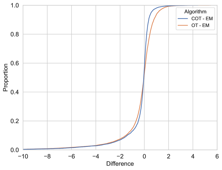
(a) Position RMSE difference

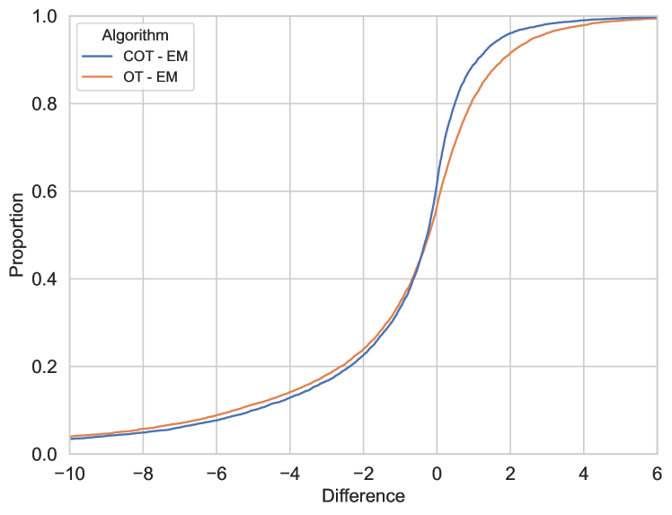
(b) Velocity RMSE difference

Figure 1: Cumulative distribution functions of RMSE differences

4.2 Pairs trading

In finance, one classic application of Kalman filters is in pairs trading. This strategy considers two stock prices, $y_{1,t}$ and $y_{2,t}$, which may be driven by many common characteristics and therefore have highly correlated stock returns. When one stock outperforms and another underperforms relative to each other, the pairs trade involves buying the under-performed stock and selling the outperformed one, with the expectation that the returns will converge and generate profits. Two stocks with strongly negative correlations can be considered similarly.

To quantify the relationship between two stocks, we employ a linear regression model with time-varying intercept and slope:

$$y_{1,t}=\alpha_{t}+\beta_{t}y_{2,t}+\varepsilon_{t}.$$

Since the intercept $\alpha_{t}$ and the slope $\beta_{t}$ are unknown, we treat them as unobservable state variables and assume a parsimonious dynamic as

$$\alpha_{t}=\alpha_{t-1}+\eta_{1,t},\quad\beta_{t}=\beta_{t-1}+\eta_{2,t},$$

where $\eta_{1,t}$ and $\eta_{2,t}$ are process noises.

Therefore, with the language of Kalman filters, the state transition matrix is $A_{t}=I_{2}$. Note that the linear regression model can be interpreted as

$$y_{1,t}=\pNiceMatrix 1&y_{2,t}\pNiceMatrix\alpha_{t}\\ \beta_{t}+\varepsilon_{t}.$$

Then the observation matrix $C_{t}=(1,y_{2,t})$. Indeed, the real noise covariance matrices are unknown. We assume the reference noise covariance matrices as $B_{t}=I_{2}$ and $D_{t}=1$, which may lead to misspecification.

The trader believes the spread, given by

$$y_{1,t}-\alpha_{t}-\beta_{t}y_{2,t},$$

is mean-reverting. Thus, when the spread exceeds the historical mean plus two standard deviations, for example, it’s considered higher than usual and the trader believes that the spread will decrease in the future. To profit from this expected mean-reversion, the trader can execute a pairs trade by longing $\beta_{t}$ shares of stock $y_{2}$ and short-selling one share of stock $y_{1}$. If the spread is too low, the trader would trade oppositely. When the spread returns to the historical mean level, the trader closes the position and realizes a profit. However, if the spread does not revert back to the mean level for an extended period, the trader may be forced to close the position and incur a loss.

We analyze the daily close prices of Google (Alphabet) and Amazon from August 9, 2019 to January 26, 2023, which comprises a total of 873 trading days. Using the first 100 days of data in 2019, we estimate the initial intercept $\alpha_{0}$ and slope $\beta_{0}$. Our portfolio starts with an initial wealth of $\$10000$. We take advantage of the mean-reverting behavior in the spread between the two stocks. When the spread deviates more than 2.0 standard deviations from its mean, we buy or sell $100\times(1,-\beta_{t})$ shares. The mean and standard deviation are calculated using a rolling window method with a window size of 20. As a result, the trade can commence on the 21st trading day of 2021. Assume the transaction cost is 0.01% of the value traded.

We consider a set of radii, ranging from 0.1 to 1.0 with a step size of 0.1, for the Wasserstein ball. The annualized Sharpe and Sortino ratios are commonly used performance measures to evaluate investment strategies. Higher ratios indicate better performance and the Sortino ratio considers the downside risk only. Table 3 presents the annualized ratios for individual stocks and the non-robust strategy, which utilizes the Kalman filter directly. For the sake of simplicity, we assume a 2% annual risk-free interest rate for this period.

Table 4 demonstrates that both the OT and COT strategies can enhance the portfolio performance by selecting an appropriate radius. In the ten choices of radii, six instances under the COT method and two instances under the OT method outperform the non-robust approach. In most cases, the COT method also outperforms the OT framework, thanks to the bi-causality constraint.

	Non-robust	GOOG	AMZN
Sharpe	0.9090	0.4671	0.1813
Sortino	2.2069	0.6545	0.2657

Table 3: Annual Sharpe and Sortino ratios of stocks and the non-robust strategy

Radius	0.1	0.2	0.3	0.4	0.5	0.6	0.7	0.8	0.9	1.0
COT Sharpe	0.8432	0.8953	0.9494	0.8973	1.0968	0.8981	1.07	1.0703	1.1322	1.1905
OT Sharpe	0.9062	0.9	0.8408	0.484	0.599	0.8284	0.8372	0.9145	1.0568	0.6908
COT Sortino	2.0257	2.0982	2.3016	2.1601	2.7703	2.1588	2.863	2.7822	2.8389	3.0438
OT Sortino	2.1341	2.1831	2.1723	1.0761	1.2958	1.9475	1.9682	2.2369	2.4592	1.5942

Table 4: Annual Sharpe and Sortino ratios of the OT and COT methods

Appendix A Proofs of results

A.1 Proof of Corollary 2.1

Define the centralized random variables as $\eta_{1}:=\xi_{1}-m_{1}\sim\tilde{\mathbb{P}}_{1}=N(0,M_{1})$ and $\eta_{2}:=\xi_{2}-m_{2}\sim\tilde{\mathbb{P}}_{2}=N(0,M_{2})$. Then the integrand reduces to

$$\xi_{1}^{\top}P\xi_{1}+\xi_{2}^{\top}Q\xi_{2}+\xi_{1}^{\top}R\xi_{2}$$

$$\qquad=(\eta_{1}+m_{1})^{\top}P(\eta_{1}+m_{1})+(\eta_{2}+m_{2})^{\top}Q(\eta_{2}+m_{2})+(\eta_{1}+m_{1})^{\top}R(\eta_{2}+m_{2})$$

$$\qquad=\eta_{1}^{\top}P\eta_{1}+\eta_{1}^{\top}Pm_{1}+m^{\top}_{1}P\eta_{1}+m^{\top}_{1}Pm_{1}$$

$$\qquad\quad+\eta_{2}^{\top}Q\eta_{2}+m_{2}^{\top}Q\eta_{2}+\eta_{2}^{\top}Qm_{2}+m_{2}^{\top}Qm_{2}$$

$$\qquad\quad+\eta_{1}^{\top}R\eta_{2}+m_{1}^{\top}R\eta_{2}+\eta_{1}^{\top}Rm_{2}+m_{1}^{\top}Rm_{2}.$$

We only need to calculate the OT problem with two zero-mean distributions, that is,

$$\inf_{\pi\in\Pi(\tilde{\mathbb{P}}_{1},\tilde{\mathbb{P}}_{2})}\int(\eta_{1}^{\top}P\eta_{1}+\eta_{2}^{\top}Q\eta_{2}+\eta_{1}^{\top}R\eta_{2})d\pi={\rm{tr}}[PM_{1}]+{\rm{tr}}[QM_{2}]+\inf_{\pi\in\Pi(\tilde{\mathbb{P}}_{1},\tilde{\mathbb{P}}_{2})}\int\eta_{1}^{\top}R\eta_{2}d\pi.$$

For the last minimization problem, we can regard $R\eta_{2}$ as a new normal random variable and apply Givens and Shortt, (1984) to $\eta_{1}$ and $R\eta_{2}$ to show that

$$\inf_{\pi\in\Pi(\tilde{\mathbb{P}}_{1},\tilde{\mathbb{P}}_{2})}\int\eta_{1}^{\top}R\eta_{2}d\pi=-{\rm{tr}}\left[\sqrt{\sqrt{M_{1}}RM_{2}R\sqrt{M_{1}}}\right].$$

∎

A.2 Proof of Corollary 2.2

By Backhoff-Veraguas et al., (2017, Proposition 5.2), the bi-causal Wasserstein distance (2.8) can be solved using the dynamic programming principle. The boundary condition implies the value function in Step 2 is

$$v_{2}=c=\|x_{t-1}-\bar{x}_{t-1}\|^{2}+\|x_{t}-\bar{x}_{t}\|^{2}+\|y_{t}-\bar{y}_{t}\|^{2}.$$

In Step 1, we obtain the value function

$$v_{1} =\inf_{\pi_{t}\in\Pi(\mathbb{P}(x_{t},y_{t}|x_{t-1},y_{1:t-1}),\mathbb{Q}(\bar{x}_{t},\bar{y}_{t}|\bar{x}_{t-1},y_{1:t-1}))}\int v_{2}d\pi_{t}$$

$$=\|x_{t-1}-\bar{x}_{t-1}\|^{2}+\inf_{\pi_{t}\in\Pi(\mathbb{P}(x_{t},y_{t}|x_{t-1}),\mathbb{Q}(\bar{x}_{t},\bar{y}_{t}|\bar{x}_{t-1}))}\int\left(\|x_{t}-\bar{x}_{t}\|^{2}+\|y_{t}-\bar{y}_{t}\|^{2}\right)d\pi_{t},$$

by the Markov property of the reference and alternative models, i.e., $\mathbb{P}(x_{t},y_{t}|x_{t-1},y_{1:t-1})=\mathbb{P}(x_{t},y_{t}|x_{t-1})$ and $\mathbb{Q}(\bar{x}_{t},\bar{y}_{t}|\bar{x}_{t-1},y_{1:t-1})=\mathbb{Q}(\bar{x}_{t},\bar{y}_{t}|\bar{x}_{t-1})$. By Corollary 2.1, with two Gaussian distributions $\xi_{1}=(x^{\top}_{t},y^{\top}_{t})^{\top}$ and $\xi_{2}=(\bar{x}^{\top}_{t},\bar{y}^{\top}_{t})^{\top}$, and coefficients $P=I_{n+m}$, $Q=I_{n+m}$, $R=-2I_{n+m}$, we obtain

$$v_{1}= \|x_{t-1}-\bar{x}_{t-1}\|^{2}+\begin{pmatrix}x^{\top}_{t-1}A^{\top}_{t},x^{\top}_{t-1}A^{\top}_{t}C^{\top}_{t}\end{pmatrix}\begin{pmatrix}A_{t}x_{t-1}\\ C_{t}A_{t}x_{t-1}\end{pmatrix}$$

$$+\begin{pmatrix}\bar{x}^{\top}_{t-1}A^{\top}_{t},\bar{x}^{\top}_{t-1}A^{\top}_{t}C^{\top}_{t}\end{pmatrix}\begin{pmatrix}A_{t}\bar{x}_{t-1}\\ C_{t}A_{t}\bar{x}_{t-1}\end{pmatrix}-2\begin{pmatrix}x^{\top}_{t-1}A^{\top}_{t},x^{\top}_{t-1}A^{\top}_{t}C^{\top}_{t}\end{pmatrix}\begin{pmatrix}A_{t}\bar{x}_{t-1}\\ C_{t}A_{t}\bar{x}_{t-1}\end{pmatrix}$$

$$+{\rm{tr}}\left[\sigma^{2}(B_{t},D_{t})+\sigma^{2}(\bar{B}_{t},\bar{D}_{t})-2\sqrt{\sqrt{\sigma^{2}(B_{t},D_{t})}\sigma^{2}(\bar{B}_{t},\bar{D}_{t})\sqrt{\sigma^{2}(B_{t},D_{t})}}\right].$$

With the definition of $H$, applying Corollary 2.1 again yields

$${\mathcal{W}}_{bc}(\mathbb{P}_{t-1},\mathbb{Q}_{t-1})= v_{0}=\inf_{\pi_{t-1}\in\Pi(\mathbb{P}(x_{t-1}|y_{1:t-1}),\mathbb{Q}(\bar{x}_{t-1}|y_{1:t-1}))}\int v_{1}d\pi_{t-1}$$

$$= \hat{x}^{\top}_{t-1}H\hat{x}_{t-1}+\hat{x}^{\top}_{t-1}H\hat{x}_{t-1}-2\hat{x}^{\top}_{t-1}H\hat{x}_{t-1}$$

$$+{\rm{tr}}\left[\sigma^{2}(B_{t},D_{t})+\sigma^{2}(\bar{B}_{t},\bar{D}_{t})-2\sqrt{\sqrt{\sigma^{2}(B_{t},D_{t})}\sigma^{2}(\bar{B}_{t},\bar{D}_{t})\sqrt{\sigma^{2}(B_{t},D_{t})}}\right]$$

$$+{\rm{tr}}\left[H\Sigma_{t-1}+H\bar{\Sigma}_{t-1}-2\sqrt{\sqrt{\Sigma_{t-1}}H\bar{\Sigma}_{t-1}H\sqrt{\Sigma_{t-1}}}\right]=:w(\bar{B}_{t},\bar{D}_{t},\bar{\Sigma}_{t-1}).$$

∎

A.3 Proof of Theorem 3.1

First, we prove the infimum and supremum in the problem (2.9) are interchangeable. Moreover, the infimum over $f\in{\mathcal{L}}$ can be restricted to linear functions.

By the weak duality and the fact that the optimizer is linear when $\mathbb{Q}$ is fixed, we obtain

$$\inf_{f\in{\mathcal{L}}}\sup_{\mathbb{Q}\in\mathcal{B}_{\varepsilon,t-1}}\mathbb{E}_{\mathbb{Q}}\left[\|\bar{x}_{t}-f(\bar{y}_{t})\|^{2}\Big{|}y_{1:t-1}\right] \geq\sup_{\mathbb{Q}\in\mathcal{B}_{\varepsilon,t-1}}\inf_{f\in{\mathcal{L}}}\mathbb{E}_{\mathbb{Q}}\left[\|\bar{x}_{t}-f(\bar{y}_{t})\|^{2}\Big{|}y_{1:t-1}\right]$$

$$=\sup_{\mathbb{Q}\in\mathcal{B}_{\varepsilon,t-1}}\inf_{G,g}\mathbb{E}_{\mathbb{Q}}\left[\|\bar{x}_{t}-G\bar{y}_{t}-g\|^{2}\Big{|}y_{1:t-1}\right].$$

Moreover, since a linear estimator is in ${\mathcal{L}}$, then

$$\inf_{f\in{\mathcal{L}}}\sup_{\mathbb{Q}\in\mathcal{B}_{\varepsilon,t-1}}\mathbb{E}_{\mathbb{Q}}\left[\|\bar{x}_{t}-f(\bar{y}_{t})\|^{2}\Big{|}y_{1:t-1}\right] \leq\inf_{G,g}\sup_{\mathbb{Q}\in\mathcal{B}_{\varepsilon,t-1}}\mathbb{E}_{\mathbb{Q}}\left[\|\bar{x}_{t}-G\bar{y}_{t}-g\|^{2}\Big{|}y_{1:t-1}\right].$$

If we can prove the strong duality for linear estimators, that is,

$$\sup_{\mathbb{Q}\in\mathcal{B}_{\varepsilon,t-1}}\inf_{G,g}\mathbb{E}_{\mathbb{Q}}\left[\|\bar{x}_{t}-G\bar{y}_{t}-g\|^{2}\Big{|}y_{1:t-1}\right] =\inf_{G,g}\sup_{\mathbb{Q}\in\mathcal{B}_{\varepsilon,t-1}}\mathbb{E}_{\mathbb{Q}}\left[\|\bar{x}_{t}-G\bar{y}_{t}-g\|^{2}\Big{|}y_{1:t-1}\right],$$ (A.1)

then all inequalities above are equalities and in particular,

$$\inf_{f\in{\mathcal{L}}}\sup_{\mathbb{Q}\in\mathcal{B}_{\varepsilon,t-1}}\mathbb{E}_{\mathbb{Q}}\left[\|\bar{x}_{t}-f(\bar{y}_{t})\|^{2}\Big{|}y_{1:t-1}\right]=\sup_{\mathbb{Q}\in\mathcal{B}_{\varepsilon,t-1}}\inf_{G,g}\mathbb{E}_{\mathbb{Q}}\left[\|\bar{x}_{t}-G\bar{y}_{t}-g\|^{2}\Big{|}y_{1:t-1}\right].$$ (A.2)

To prove the strong duality (A.1), we invoke Sion’s minimax theorem. Note that $\mathbb{Q}$ is fully characterized by the choice of $\bar{B}_{t},\bar{D}_{t},\bar{\Sigma}_{t-1}$. With a given $\mathbb{Q}$, we have

$$\mathbb{E}_{\mathbb{Q}}[\bar{x}^{\top}_{t}\bar{x}_{t}|y_{1:t-1}]= \hat{x}^{\top}_{t-1}A^{\top}_{t}A_{t}\hat{x}_{t-1}+{\rm{tr}}[A_{t}\bar{\Sigma}_{t-1}A^{\top}_{t}+\bar{B}_{t}],$$

$$\mathbb{E}_{\mathbb{Q}}[\bar{y}^{\top}_{t}G^{\top}G\bar{y}_{t}|y_{1:t-1}]= \hat{x}^{\top}_{t-1}A^{\top}_{t}C^{\top}_{t}G^{\top}GC_{t}A_{t}\hat{x}_{t-1}+{\rm{tr}}[C_{t}A_{t}\bar{\Sigma}_{t-1}A^{\top}_{t}C^{\top}_{t}G^{\top}G]$$

$$+{\rm{tr}}[(C_{t}\bar{B}_{t}C^{\top}_{t}+\bar{D}_{t})G^{\top}G],$$

$$\mathbb{E}_{\mathbb{Q}}[\bar{y}^{\top}_{t}G^{\top}\bar{x}_{t}|y_{1:t-1}]= \mathbb{E}_{\mathbb{Q}}[\bar{x}^{\top}_{t}G\bar{y}_{t}|y_{1:t-1}]$$

$$= \hat{x}^{\top}_{t-1}A^{\top}_{t}GC_{t}A_{t}\hat{x}_{t-1}+{\rm{tr}}[(C_{t}A_{t}\bar{\Sigma}_{t-1}A^{\top}_{t}+C_{t}\bar{B}_{t})G],$$

$$\mathbb{E}_{\mathbb{Q}}[\bar{y}^{\top}_{t}G^{\top}g|y_{1:t-1}]= \mathbb{E}_{\mathbb{Q}}[g^{\top}G\bar{y}_{t}|y_{1:t-1}]=\hat{x}^{\top}_{t-1}A^{\top}_{t}C^{\top}_{t}G^{\top}g,$$

$$\mathbb{E}_{\mathbb{Q}}[g^{\top}\bar{x}_{t}|y_{1:t-1}]= \mathbb{E}_{\mathbb{Q}}[\bar{x}^{\top}_{t}g|y_{1:t-1}]=\hat{x}^{\top}_{t-1}A^{\top}_{t}g.$$

Then we verify the conditions for Sion’s minimax theorem.

1. When written in a matrix form, the objective is linear and thus quasi-concave in $\bar{B}_{t},\bar{D}_{t},\bar{\Sigma}_{t-1}$. Besides, it is convex and thus quasi-convex in $G,g$.

2. The domain for $G,g$ is convex.

3. Since the set $\{\bar{B}_{t}\succeq 0,\bar{D}_{t}\succeq\delta I_{m},\bar{\Sigma}_{t-1}\succeq 0\}$ is closed and convex, we only need to prove the set $\{w(\bar{B}_{t},\bar{D}_{t},\bar{\Sigma}_{t-1})\leq\varepsilon\}$ is compact and convex. Noting that the trace operator is linear and $\sigma^{2}(\bar{B}_{t},\bar{D}_{t})$ is linear in $(\bar{B}_{t},\bar{D}_{t})$, it suffices to show that the function ${\rm{tr}}[\sqrt{(\cdot)}]$ is concave. Consider two positive semi-definite matrices $X$ and $Y$. We want to show

   $${\rm{tr}}[\sqrt{\lambda X+(1-\lambda)Y}]\geq\lambda{\rm{tr}}[\sqrt{X}]+(1-\lambda){\rm{tr}}[\sqrt{Y}].$$

   Equivalently, we need to prove

   $$\sqrt{\lambda X+(1-\lambda)Y}\succeq\lambda\sqrt{X}+(1-\lambda)\sqrt{Y}.$$

   Indeed, the square root is monotone for positive semi-definite matrices. Moreover,

   $$\lambda X+(1-\lambda)Y-(\lambda\sqrt{X}+(1-\lambda)\sqrt{Y})(\lambda\sqrt{X}+(1-\lambda)\sqrt{Y})$$

   $$\qquad=\lambda(1-\lambda)(X+Y-\sqrt{X}\sqrt{Y}-\sqrt{Y}\sqrt{X})\succeq 0.$$

   Then $w(\bar{B}_{t},\bar{D}_{t},\bar{\Sigma}_{t-1})$ is convex and $w(\bar{B}_{t},\bar{D}_{t},\bar{\Sigma}_{t-1})\leq\varepsilon$ is a convex set. It is straightforward to see the set is compact.

Conditions in Sion’s minimax theorem are verified. Hence, (A.1) and (A.2) hold.

Next, we further simplify the right-hand side of (A.2). Minimizing over $g$ and setting the first derivative to be zero, we obtain

$$g_{*}=A_{t}\hat{x}_{t-1}-GC_{t}A_{t}\hat{x}_{t-1}.$$

On the right-hand side of (A.2), terms depending on $g_{*}$ become

$$(g_{*})^{\top}g_{*}+2\hat{x}^{\top}_{t-1}A^{\top}_{t}C^{\top}_{t}G^{\top}g_{*}-2\hat{x}^{\top}_{t-1}A^{\top}_{t}g_{*}$$

$$\qquad=-\hat{x}^{\top}_{t-1}A^{\top}_{t}A_{t}\hat{x}_{t-1}+\hat{x}^{\top}_{t-1}A^{\top}_{t}C^{\top}_{t}G^{\top}A_{t}\hat{x}_{t-1}$$

$$\qquad\quad+\hat{x}^{\top}_{t-1}A^{\top}_{t}GC_{t}A_{t}\hat{x}_{t-1}-\hat{x}^{\top}_{t-1}A^{\top}_{t}C^{\top}_{t}G^{\top}GC_{t}A_{t}\hat{x}_{t-1}.$$

The objective $\mathbb{E}_{\mathbb{Q}}\left[\|\bar{x}_{t}-G\bar{y}_{t}-g\|^{2}\Big{|}y_{1:t-1}\right]$ with $g_{*}$ is given by

$${\rm{tr}}[A_{t}\bar{\Sigma}_{t-1}A^{\top}_{t}+\bar{B}_{t}]+{\rm{tr}}[C_{t}A_{t}\bar{\Sigma}_{t-1}A^{\top}_{t}C^{\top}_{t}G^{\top}G]$$

$$+{\rm{tr}}[(C_{t}\bar{B}_{t}C^{\top}_{t}+\bar{D}_{t})G^{\top}G]-{\rm{tr}}[(C_{t}A_{t}\bar{\Sigma}_{t-1}A^{\top}_{t}+C_{t}\bar{B}_{t})G]$$

$$-{\rm{tr}}[G^{\top}(A_{t}\bar{\Sigma}_{t-1}A^{\top}_{t}C^{\top}_{t}+\bar{B}_{t}C^{\top}_{t})].$$

Or in a matrix form, it becomes

$${\rm{tr}}\left[\begin{pmatrix}A_{t}\bar{\Sigma}_{t-1}A^{\top}_{t}+\bar{B}_{t},&A_{t}\bar{\Sigma}_{t-1}A^{\top}_{t}C^{\top}_{t}+\bar{B}_{t}C^{\top}_{t}\\ C_{t}A_{t}\bar{\Sigma}_{t-1}A^{\top}_{t}+C_{t}\bar{B}_{t},&C_{t}A_{t}\bar{\Sigma}_{t-1}A^{\top}_{t}C^{\top}_{t}+C_{t}\bar{B}_{t}C^{\top}_{t}+\bar{D}_{t}\end{pmatrix}\begin{pmatrix}I_{n},&-G\\ -G^{\top},&G^{\top}G\end{pmatrix}\right].$$ (A.3)

To minimize over $G$, note that $\bar{D}_{t}\succeq\delta I_{m}$ with a given sufficiently small $\delta>0$. Thus, the objective (A.3) is strictly convex in $G$. The minimization problem over $G$ has a unique solution $G_{*}$, which can be solved from the first-order optimality condition:

$$2G_{*}K-2M^{\top}=0.$$

Therefore, $G_{*}=M^{\top}K^{-1}$. Substituting $G_{*}$ into the objective (A.3), we obtain (3.1). The robust optimizer (3.2) is proved with the expressions of $G_{*}$ and $g_{*}$. ∎

A.4 Proof of Lemma 3.2

The idea is to investigate the Hessian matrix of the objective function $F$ in (3.1). Since ${\rm{tr}}[A_{t}\bar{\Sigma}_{t-1}A^{\top}_{t}+\bar{B}_{t}]$ is linear, we only need to show the Hessian of ${\rm{tr}}[MM^{\top}K^{-1}]$ is positive semi-definite. We omit the time subscript for simplicity.

Derivatives on $\bar{B}$

As ${\rm{tr}}[M^{\top}K^{-1}M]=\sum_{r}(M^{\top}K^{-1}M)_{rr}$, we have

$$\frac{\partial}{\partial\bar{B}_{ij}}(M^{\top}K^{-1}M)_{rr}=\frac{\partial}{\partial\bar{B}_{ij}}\sum_{w,x}(M^{\top})_{rw}(K^{-1})_{wx}M_{xr}$$

$$\qquad=\sum_{w,x}\frac{\partial(M^{\top})_{rw}}{\partial\bar{B}_{ij}}(K^{-1})_{wx}M_{xr}+(M^{\top})_{rw}\frac{\partial(K^{-1})_{wx}}{\partial\bar{B}_{ij}}M_{xr}+(M^{\top})_{rw}(K^{-1})_{wx}\frac{\partial M_{xr}}{\partial\bar{B}_{ij}}.$$

Since $M_{xr}=\text{constant}+\sum_{z}C_{xz}\bar{B}_{zr}$, then

$$\frac{\partial M_{xr}}{\partial\bar{B}_{ij}}=C_{xi}\delta_{rj},\quad\frac{\partial(M^{\top})_{rw}}{\partial\bar{B}_{ij}}=C_{wi}\delta_{rj},$$

where $\delta_{rj}$ is the Kronecker delta.

By the formula for the derivative of matrix inverse, see Petersen and Pedersen, (2012, Equation 60), we have

$$\frac{\partial(K^{-1})_{wx}}{\partial\bar{B}_{ij}} =\sum_{v,z}\frac{\partial(K^{-1})_{wx}}{\partial K_{vz}}\frac{\partial K_{vz}}{\partial\bar{B}_{ij}}=-\sum_{v,z}(K^{-1})_{wv}(K^{-1})_{zx}C_{vi}(C^{\top})_{jz}$$

$$=-(K^{-1}C)_{wi}(C^{\top}K^{-1})_{jx}.$$

Then

$$\frac{\partial}{\partial\bar{B}_{ij}}(M^{\top}K^{-1}M)_{rr}$$

$$\qquad=\sum_{w,x}C_{wi}\delta_{rj}(K^{-1})_{wx}M_{xr}-\sum_{v,z,w,x}(M^{\top})_{rw}(K^{-1})_{wv}(K^{-1})_{zx}C_{vi}(C^{\top})_{jz}M_{xr}$$

$$\qquad\quad+\sum_{w,x}(M^{\top})_{rw}(K^{-1})_{wx}C_{xi}\delta_{rj}.$$

Next, we sum over $r$ and rearrange terms in an order of matrix multiplication. Since $K^{-1}$ is symmetric, we obtain

$$\frac{\partial}{\partial\bar{B}_{ij}}{\rm{tr}}[M^{\top}K^{-1}M]$$

$$\qquad=2\sum_{w,x}(C^{\top})_{iw}(K^{-1})_{wx}M_{xj}-\sum_{r,v,z,w,x}(C^{\top})_{iv}(K^{-1})_{vw}M_{wr}(M^{\top})_{rx}(K^{-1})_{xz}C_{zj}.$$

For the second derivatives with respect to $\bar{B}$, we have

$$\frac{\partial^{2}}{\partial\bar{B}_{ij}\partial\bar{B}_{kl}}{\rm{tr}}[M^{\top}K^{-1}M]$$

$$\qquad=-2\sum_{w,x}(C^{\top})_{iw}(K^{-1}C)_{wk}(C^{\top}K^{-1})_{lx}M_{xj}+2\sum_{w,x}(C^{\top})_{iw}(K^{-1})_{wx}C_{xk}\delta_{lj}$$

$$\qquad\quad-\sum_{r,v,z,w,x}(C^{\top})_{iv}(-1)(K^{-1}C)_{vk}(C^{\top}K^{-1})_{lw}M_{wr}(M^{\top})_{rx}(K^{-1})_{xz}C_{zj}$$

$$\qquad\quad-\sum_{r,v,z,w,x}(C^{\top})_{iv}(K^{-1})_{vw}C_{wk}\delta_{lr}(M^{\top})_{rx}(K^{-1})_{xz}C_{zj}$$

$$\qquad\quad-\sum_{r,v,z,w,x}(C^{\top})_{iv}(K^{-1})_{vw}M_{wr}C_{xk}\delta_{lr}(K^{-1})_{xz}C_{zj}$$

$$\qquad\quad-\sum_{r,v,z,w,x}(C^{\top})_{iv}(K^{-1})_{vw}M_{wr}(M^{\top})_{rx}(-1)(K^{-1}C)_{xk}(C^{\top}K^{-1})_{lz}C_{zj}$$

$$\qquad=-2(C^{\top}K^{-1}C)_{ik}(C^{\top}K^{-1}M)_{lj}+2(C^{\top}K^{-1}C)_{ik}\delta_{lj}$$

$$\qquad\quad+(C^{\top}K^{-1}C)_{ik}(C^{\top}K^{-1}MM^{\top}K^{-1}C)_{lj}-(C^{\top}K^{-1}C)_{ik}(M^{\top}K^{-1}C)_{lj}$$

$$\qquad\quad-(C^{\top}K^{-1}M)_{il}(C^{\top}K^{-1}C)_{kj}+(C^{\top}K^{-1}MM^{\top}K^{-1}C)_{ik}(C^{\top}K^{-1}C)_{lj}.$$

Besides,

$$\frac{\partial^{2}}{\partial\bar{B}_{ij}\partial\bar{\Sigma}_{kl}}{\rm{tr}}[M^{\top}K^{-1}M]$$

$$\qquad=-2\sum_{w,x}(C^{\top})_{iw}(K^{-1}CA)_{wk}(A^{\top}C^{\top}K^{-1})_{lx}M_{xj}+2\sum_{w,x}(C^{\top})_{iw}(K^{-1})_{wx}(CA)_{xk}(A^{\top})_{lj}$$

$$\qquad\quad-\sum_{r,v,z,w,x}(C^{\top})_{iv}(-1)(K^{-1}CA)_{vk}(A^{\top}C^{\top}K^{-1})_{lw}M_{wr}(M^{\top})_{rx}(K^{-1})_{xz}C_{zj}$$

$$\qquad\quad-\sum_{r,v,z,w,x}(C^{\top})_{iv}(K^{-1})_{vw}(CA)_{wk}(A^{\top})_{lr}(M^{\top})_{rx}(K^{-1})_{xz}C_{zj}$$

$$\qquad\quad-\sum_{r,v,z,w,x}(C^{\top})_{iv}(K^{-1})_{vw}M_{wr}(CA)_{xk}(A^{\top})_{lr}(K^{-1})_{xz}C_{zj}$$

$$\qquad\quad-\sum_{r,v,z,w,x}(C^{\top})_{iv}(K^{-1})_{vw}M_{wr}(M^{\top})_{rx}(-1)(K^{-1}CA)_{xk}(A^{\top}C^{\top}K^{-1})_{lz}C_{zj}$$

$$\qquad=-2(C^{\top}K^{-1}CA)_{ik}(A^{\top}C^{\top}K^{-1}M)_{lj}+2(C^{\top}K^{-1}CA)_{ik}(A^{\top})_{lj}$$

$$\qquad\quad+(C^{\top}K^{-1}CA)_{ik}(A^{\top}C^{\top}K^{-1}MM^{\top}K^{-1}C)_{lj}-(C^{\top}K^{-1}CA)_{ik}(A^{\top}M^{\top}K^{-1}C)_{lj}$$

$$\qquad\quad-(C^{\top}K^{-1}MA)_{il}(A^{\top}C^{\top}K^{-1}C)_{kj}+(C^{\top}K^{-1}MM^{\top}K^{-1}CA)_{ik}(A^{\top}C^{\top}K^{-1}C)_{lj}.$$

Derivatives on $\bar{D}$

Note that $\bar{D}$ appears only in $K$. The first derivative is

$$\frac{\partial}{\partial\bar{D}_{ij}}{\rm{tr}}[M^{\top}K^{-1}M]=-\sum_{w,x,y}(K^{-1})_{iw}M_{wx}(M^{\top})_{xy}(K^{-1})_{yj}.$$

The second derivatives are

$$\frac{\partial^{2}}{\partial\bar{D}_{ij}\partial\bar{D}_{kl}}{\rm{tr}}[M^{\top}K^{-1}M]= -\sum_{w,x,y}(-1)(K^{-1})_{ik}(K^{-1})_{wl}M_{wx}(M^{\top})_{xy}(K^{-1})_{yj}$$

$$-\sum_{w,x,y}(-1)(K^{-1})_{iw}M_{wx}(M^{\top})_{xy}(K^{-1})_{yk}(K^{-1})_{lj}$$

$$= (K^{-1})_{ik}(K^{-1}MM^{\top}K^{-1})_{lj}+(K^{-1}MM^{\top}K^{-1})_{ik}(K^{-1})_{lj}$$

and

$$\frac{\partial^{2}}{\partial\bar{D}_{ij}\partial\bar{B}_{kl}}{\rm{tr}}[M^{\top}K^{-1}M]= \sum_{w,x,y}(K^{-1}C)_{ik}(C^{\top}K^{-1})_{lw}M_{wx}(M^{\top})_{xy}(K^{-1})_{yj}$$

$$-\sum_{w,x,y}(K^{-1})_{iw}C_{wk}\delta_{lx}(M^{\top})_{xy}(K^{-1})_{yj}$$

$$-\sum_{w,x,y}(K^{-1})_{iw}M_{wx}C_{yk}\delta_{lx}(K^{-1})_{yj}$$

$$+\sum_{w,x,y}(K^{-1})_{iw}M_{wx}(M^{\top})_{xy}(K^{-1}C)_{yk}(C^{\top}K^{-1})_{lj}$$

$$= (K^{-1}C)_{ik}(C^{\top}K^{-1}MM^{\top}K^{-1})_{lj}-(K^{-1}C)_{ik}(M^{\top}K^{-1})_{lj}$$

$$-(C^{\top}K^{-1})_{kj}(K^{-1}M)_{il}+(K^{-1}MM^{\top}K^{-1}C)_{ik}(C^{\top}K^{-1})_{lj}.$$

With

$$\frac{\partial(K^{-1})_{iw}}{\partial\bar{\Sigma}_{kl}}=-(K^{-1}CA)_{ik}(A^{\top}C^{\top}K^{-1})_{lw},\quad\frac{\partial M_{wx}}{\partial\bar{\Sigma}_{kl}}=(CA)_{wk}(A^{\top})_{lx},$$

we obtain

$$\frac{\partial^{2}}{\partial\bar{D}_{ij}\partial\bar{\Sigma}_{kl}}{\rm{tr}}[M^{\top}K^{-1}M]$$

$$\qquad=\sum_{w,x,y}(K^{-1}CA)_{ik}(A^{\top}C^{\top}K^{-1})_{lw}M_{wx}(M^{\top})_{xy}(K^{-1})_{yj}$$

$$\qquad\quad-\sum_{w,x,y}(K^{-1})_{iw}(CA)_{wk}(A^{\top})_{lx}(M^{\top})_{xy}(K^{-1})_{yj}$$

$$\qquad\quad-\sum_{w,x,y}(K^{-1})_{iw}M_{wx}(CA)_{yk}(A^{\top})_{lx}(K^{-1})_{yj}$$

$$\qquad\quad+\sum_{w,x,y}(K^{-1})_{iw}M_{wx}(M^{\top})_{xy}(K^{-1}CA)_{yk}(A^{\top}C^{\top}K^{-1})_{lj}$$

$$\qquad=(K^{-1}CA)_{ik}(A^{\top}C^{\top}K^{-1}MM^{\top}K^{-1})_{lj}-(K^{-1}CA)_{ik}(A^{\top}M^{\top}K^{-1})_{lj}$$

$$\qquad\quad-(A^{\top}C^{\top}K^{-1})_{kj}(K^{-1}MA)_{il}+(K^{-1}MM^{\top}K^{-1}CA)_{ik}(A^{\top}C^{\top}K^{-1})_{lj}.$$

Derivatives on $\bar{\Sigma}$

$\bar{\Sigma}$ appears in a similar position of $\bar{B}$. Therefore,

$$\frac{\partial}{\partial\bar{\Sigma}_{ij}}{\rm{tr}}[M^{\top}K^{-1}M]= 2\sum_{w,x,y}(A^{\top}C^{\top})_{iw}(K^{-1})_{wx}M_{xy}A_{yj}$$

$$-\sum_{r,v,z,w,x}(A^{\top}C^{\top})_{iv}(K^{-1})_{vw}M_{wr}(M^{\top})_{rx}(K^{-1})_{xz}(CA)_{zj}.$$

For the second derivatives, we have

$$\frac{\partial^{2}}{\partial\bar{\Sigma}_{ij}\partial\bar{\Sigma}_{kl}}{\rm{tr}}[M^{\top}K^{-1}M]= -2(A^{\top}C^{\top}K^{-1}CA)_{ik}(A^{\top}C^{\top}K^{-1}MA)_{lj}$$

$$+2(A^{\top}C^{\top}K^{-1}CA)_{ik}(A^{\top}A)_{lj}$$

$$+(A^{\top}C^{\top}K^{-1}CA)_{ik}(A^{\top}C^{\top}K^{-1}MM^{\top}K^{-1}CA)_{lj}$$

$$-(A^{\top}C^{\top}K^{-1}CA)_{ik}(A^{\top}M^{\top}K^{-1}CA)_{lj}$$

$$-(A^{\top}C^{\top}K^{-1}MA)_{il}(A^{\top}C^{\top}K^{-1}CA)_{kj}$$

$$+(A^{\top}C^{\top}K^{-1}MM^{\top}K^{-1}CA)_{ik}(A^{\top}C^{\top}K^{-1}CA)_{lj}.$$

To validate that the Hessian matrix is positive semi-definite, we take arbitrary positive semi-definite matrices $B,D,\Sigma$ and view them as double-indexed vectors. Consider the quadratic form

$$\sum_{i,j,k,l}\Big{\{} B_{ij}\frac{\partial^{2}{\rm{tr}}[M^{\top}K^{-1}M]}{\partial\bar{B}_{ij}\partial\bar{B}_{kl}}B_{kl}+B_{ij}\frac{\partial^{2}{\rm{tr}}[M^{\top}K^{-1}M]}{\partial\bar{B}_{ij}\partial\bar{D}_{kl}}D_{kl}+B_{ij}\frac{\partial^{2}{\rm{tr}}[M^{\top}K^{-1}M]}{\partial\bar{B}_{ij}\partial\bar{\Sigma}_{kl}}\Sigma_{kl}$$

$$+D_{ij}\frac{\partial^{2}{\rm{tr}}[M^{\top}K^{-1}M]}{\partial\bar{D}_{ij}\partial\bar{D}_{kl}}D_{kl}+D_{ij}\frac{\partial^{2}{\rm{tr}}[M^{\top}K^{-1}M]}{\partial\bar{D}_{ij}\partial\bar{B}_{kl}}B_{kl}+D_{ij}\frac{\partial^{2}{\rm{tr}}[M^{\top}K^{-1}M]}{\partial\bar{D}_{ij}\partial\bar{\Sigma}_{kl}}\Sigma_{kl}$$ (A.4)

$$+\Sigma_{ij}\frac{\partial^{2}{\rm{tr}}[M^{\top}K^{-1}M]}{\partial\bar{\Sigma}_{ij}\partial\bar{\Sigma}_{kl}}\Sigma_{kl}+\Sigma_{ij}\frac{\partial^{2}{\rm{tr}}[M^{\top}K^{-1}M]}{\partial\bar{\Sigma}_{ij}\partial\bar{B}_{kl}}B_{kl}+\Sigma_{ij}\frac{\partial^{2}{\rm{tr}}[M^{\top}K^{-1}M]}{\partial\bar{\Sigma}_{ij}\partial\bar{D}_{kl}}D_{kl}\Big{\}}.$$

We take the first term $B_{ij}\frac{\partial^{2}{\rm{tr}}[M^{\top}K^{-1}M]}{\partial\bar{B}_{ij}\partial\bar{B}_{kl}}B_{kl}$ as an example. We have

$$\sum_{i,j,k,l}-2(C^{\top}K^{-1}C)_{ik}B_{kl}(C^{\top}K^{-1}M)_{lj}B_{ij}= -2{\rm{tr}}\left[C^{\top}K^{-1}CBC^{\top}K^{-1}MB^{\top}\right]$$

$$= -2{\rm{tr}}\left[C^{\top}K^{-1}CBC^{\top}K^{-1}MB\right],$$

where the second equality follows from that $B$ is symmetric. Other terms can be calculated in the same way. Then

$$\sum_{i,j,k,l}B_{ij}\frac{\partial^{2}{\rm{tr}}[M^{\top}K^{-1}M]}{\partial\bar{B}_{ij}\partial\bar{B}_{kl}}B_{kl}= -2{\rm{tr}}\left[C^{\top}K^{-1}CBC^{\top}K^{-1}MB\right]+2{\rm{tr}}\left[C^{\top}K^{-1}CBB\right]$$

$$+{\rm{tr}}\left[C^{\top}K^{-1}CBC^{\top}K^{-1}MM^{\top}K^{-1}CB\right]$$

$$-{\rm{tr}}\left[C^{\top}K^{-1}CBM^{\top}K^{-1}CB\right]$$

$$-{\rm{tr}}\left[C^{\top}K^{-1}MBC^{\top}K^{-1}CB\right]$$

$$+{\rm{tr}}\left[C^{\top}K^{-1}MM^{\top}K^{-1}CBC^{\top}K^{-1}CB\right].$$

Similarly, we have the following results for other terms:

$$\sum_{i,j,k,l}D_{ij}\frac{\partial^{2}{\rm{tr}}[M^{\top}K^{-1}M]}{\partial\bar{D}_{ij}\partial\bar{D}_{kl}}D_{kl}={\rm{tr}}[K^{-1}DK^{-1}MM^{\top}K^{-1}D+K^{-1}MM^{\top}K^{-1}DK^{-1}D].$$

$$\sum_{i,j,k,l}\Sigma_{ij}\frac{\partial^{2}{\rm{tr}}[M^{\top}K^{-1}M]}{\partial\bar{\Sigma}_{ij}\partial\bar{\Sigma}_{kl}}\Sigma_{kl}= -2{\rm{tr}}[A^{\top}C^{\top}K^{-1}CA\Sigma A^{\top}C^{\top}K^{-1}MA\Sigma]$$

$$+2{\rm{tr}}[A^{\top}C^{\top}K^{-1}CA\Sigma A^{\top}A\Sigma]$$

$$+{\rm{tr}}[A^{\top}C^{\top}K^{-1}CA\Sigma A^{\top}C^{\top}K^{-1}MM^{\top}K^{-1}CA\Sigma]$$

$$-{\rm{tr}}[A^{\top}C^{\top}K^{-1}CA\Sigma A^{\top}M^{\top}K^{-1}CA\Sigma]$$

$$-{\rm{tr}}[A^{\top}C^{\top}K^{-1}MA\Sigma A^{\top}C^{\top}K^{-1}CA\Sigma]$$

$$+{\rm{tr}}[A^{\top}C^{\top}K^{-1}MM^{\top}K^{-1}CA\Sigma A^{\top}C^{\top}K^{-1}CA\Sigma].$$

$$\sum_{i,j,k,l}\Big{\{}D_{ij}\frac{\partial^{2}{\rm{tr}}[M^{\top}K^{-1}M]}{\partial\bar{D}_{ij}\partial\bar{B}_{kl}}B_{kl}+B_{ij}\frac{\partial^{2}{\rm{tr}}[M^{\top}K^{-1}M]}{\partial\bar{B}_{ij}\partial\bar{D}_{kl}}D_{kl}\Big{\}}$$

$$\qquad=2{\rm{tr}}[K^{-1}CBC^{\top}K^{-1}MM^{\top}K^{-1}D]-2{\rm{tr}}[K^{-1}CBM^{\top}K^{-1}D]$$

$$\qquad\quad-2{\rm{tr}}[C^{\top}K^{-1}DK^{-1}MB]+2{\rm{tr}}[K^{-1}MM^{\top}K^{-1}CBC^{\top}K^{-1}D].$$

$$\sum_{i,j,k,l}\Big{\{}B_{ij}\frac{\partial^{2}{\rm{tr}}[M^{\top}K^{-1}M]}{\partial\bar{B}_{ij}\partial\bar{\Sigma}_{kl}}\Sigma_{kl}+\Sigma_{ij}\frac{\partial^{2}{\rm{tr}}[M^{\top}K^{-1}M]}{\partial\bar{\Sigma}_{ij}\partial\bar{B}_{kl}}B_{kl}\Big{\}}$$

$$\qquad=-4{\rm{tr}}[C^{\top}K^{-1}CA\Sigma A^{\top}C^{\top}K^{-1}MB]+4{\rm{tr}}[C^{\top}K^{-1}CA\Sigma A^{\top}B]$$

$$\qquad\quad+2{\rm{tr}}[C^{\top}K^{-1}CA\Sigma A^{\top}C^{\top}K^{-1}MM^{\top}K^{-1}CB]$$

$$\qquad\quad-2{\rm{tr}}[C^{\top}K^{-1}CA\Sigma A^{\top}M^{\top}K^{-1}CB]$$

$$\qquad\quad-2{\rm{tr}}[C^{\top}K^{-1}MA\Sigma A^{\top}C^{\top}K^{-1}CB]$$

$$\qquad\quad+2{\rm{tr}}[C^{\top}K^{-1}MM^{\top}K^{-1}CA\Sigma A^{\top}C^{\top}K^{-1}CB].$$

$$\sum_{i,j,k,l}\Big{\{}D_{ij}\frac{\partial^{2}{\rm{tr}}[M^{\top}K^{-1}M]}{\partial\bar{D}_{ij}\partial\bar{\Sigma}_{kl}}\Sigma_{kl}+\Sigma_{ij}\frac{\partial^{2}{\rm{tr}}[M^{\top}K^{-1}M]}{\partial\bar{\Sigma}_{ij}\partial\bar{D}_{kl}}D_{kl}\Big{\}}$$

$$\qquad=2{\rm{tr}}[K^{-1}CA\Sigma A^{\top}C^{\top}K^{-1}MM^{\top}K^{-1}D]-2{\rm{tr}}[K^{-1}CA\Sigma A^{\top}M^{\top}K^{-1}D]$$

$$\qquad\quad-2{\rm{tr}}[K^{-1}MA\Sigma A^{\top}C^{\top}K^{-1}D]+2{\rm{tr}}[K^{-1}MM^{\top}K^{-1}CA\Sigma A^{\top}C^{\top}K^{-1}D].$$

Summing all terms up, we find that the quadratic form (A.4) equals to $2{\rm{tr}}[K^{-1}LL^{\top}]$ with

$$L:=DK^{-1}M+CBC^{\top}K^{-1}M-CB+CA\Sigma A^{\top}C^{\top}K^{-1}M-CA\Sigma A^{\top}.$$

It shows the Hessian matrix of ${\rm{tr}}[MM^{\top}K^{-1}]$ is positive semi-definite. ∎

References

• Acciaio et al., (2021) Acciaio, B., Backhoff-Veraguas, J., and Jia, J. (2021). Cournot–Nash equilibrium and optimal transport in a dynamic setting. SIAM Journal on Control and Optimization, 59(3):2273–2300.
• Acciaio et al., (2020) Acciaio, B., Backhoff-Veraguas, J., and Zalashko, A. (2020). Causal optimal transport and its links to enlargement of filtrations and continuous-time stochastic optimization. Stochastic Processes and their Applications, 130(5):2918–2953.
• Backhoff-Veraguas et al., (2020) Backhoff-Veraguas, J., Bartl, D., Beiglböck, M., and Eder, M. (2020). Adapted Wasserstein distances and stability in mathematical finance. Finance and Stochastics, 24(3):601–632.
• Backhoff-Veraguas et al., (2017) Backhoff-Veraguas, J., Beiglbock, M., Lin, Y., and Zalashko, A. (2017). Causal transport in discrete time and applications. SIAM Journal on Optimization, 27(4):2528–2562.
• Benson and Vanderbei, (2003) Benson, H. Y. and Vanderbei, R. J. (2003). Solving problems with semidefinite and related constraints using interior-point methods for nonlinear programming. Mathematical Programming, 95(2):279–302.
• Durovic and Kovacevic, (1999) Durovic, Z. M. and Kovacevic, B. D. (1999). Robust estimation with unknown noise statistics. IEEE Transactions on Automatic Control, 44(6):1292–1296.
• Galichon, (2016) Galichon, A. (2016). Optimal transport methods in economics. Princeton University Press.
• Gandhi and Mili, (2009) Gandhi, M. A. and Mili, L. (2009). Robust Kalman filter based on a generalized maximum-likelihood-type estimator. IEEE Transactions on Signal Processing, 58(5):2509–2520.
• Givens and Shortt, (1984) Givens, C. R. and Shortt, R. M. (1984). A class of Wasserstein metrics for probability distributions. Michigan Mathematical Journal, 31(2):231–240.
• Hansen and Sargent, (2001) Hansen, L. and Sargent, T. J. (2001). Robust control and model uncertainty. American Economic Review, 91(2):60–66.
• Hansen, (2014) Hansen, L. P. (2014). Nobel lecture: Uncertainty outside and inside economic models. Journal of Political Economy, 122(5):945–987.
• Hassibi et al., (1999) Hassibi, B., Sayed, A. H., and Kailath, T. (1999). Indefinite-quadratic estimation and control: A unified approach to $H^{2}$ and $H^{\infty}$ theories. SIAM.
• Huang et al., (2017) Huang, Y., Zhang, Y., Wu, Z., Li, N., and Chambers, J. (2017). A novel adaptive Kalman filter with inaccurate process and measurement noise covariance matrices. IEEE Transactions on Automatic Control, 63(2):594–601.
• Huang et al., (2020) Huang, Y., Zhang, Y., Zhao, Y., Shi, P., and Chambers, J. A. (2020). A novel outlier-robust Kalman filtering framework based on statistical similarity measure. IEEE Transactions on Automatic Control, 66(6):2677–2692.
• Kassam and Poor, (1985) Kassam, S. A. and Poor, H. V. (1985). Robust techniques for signal processing: A survey. Proceedings of the IEEE, 73(3):433–481.
• Lassalle, (2013) Lassalle, R. (2013). Causal transference plans and their Monge-Kantorovich problems. arXiv preprint arXiv:1303.6925.
• Levy and Nikoukhah, (2012) Levy, B. C. and Nikoukhah, R. (2012). Robust state space filtering under incremental model perturbations subject to a relative entropy tolerance. IEEE Transactions on Automatic Control, 58(3):682–695.
• Petersen and Savkin, (1999) Petersen, I. R. and Savkin, A. V. (1999). Robust Kalman filtering for signals and systems with large uncertainties. Springer Science & Business Media.
• Petersen and Pedersen, (2012) Petersen, K. B. and Pedersen, M. S. (November 15, 2012). The matrix cookbook.
• Peyré and Cuturi, (2019) Peyré, G. and Cuturi, M. (2019). Computational optimal transport: With applications to data science. Foundations and Trends® in Machine Learning, 11(5-6):355–607.
• Pflug and Pichler, (2012) Pflug, G. C. and Pichler, A. (2012). A distance for multistage stochastic optimization models. SIAM Journal on Optimization, 22(1):1–23.
• Santambrogio, (2015) Santambrogio, F. (2015). Optimal transport for applied mathematicians. Birkäuser, NY, 55(58-63):94.
• Shafieezadeh Abadeh et al., (2018) Shafieezadeh Abadeh, S., Nguyen, V. A., Kuhn, D., and Mohajerin Esfahani, P. M. (2018). Wasserstein distributionally robust Kalman filtering. Advances in Neural Information Processing Systems, 31.
• Speyer et al., (1974) Speyer, J., Deyst, J., and Jacobson, D. (1974). Optimization of stochastic linear systems with additive measurement and process noise using exponential performance criteria. IEEE Transactions on Automatic Control, 19(4):358–366.
• Taghvaei and Mehta, (2020) Taghvaei, A. and Mehta, P. G. (2020). An optimal transport formulation of the ensemble Kalman filter. IEEE Transactions on Automatic Control, 66(7):3052–3067.
• Villani, (2009) Villani, C. (2009). Optimal transport: old and new, volume 338. Springer.
• Xu and Acciaio, (2021) Xu, T. and Acciaio, B. (2021). Quantized conditional COT-GAN for video prediction. arXiv preprint arXiv:2106.05658.
• Xu et al., (2020) Xu, T., Li, W. K., Munn, M., and Acciaio, B. (2020). COT-GAN: Generating sequential data via causal optimal transport. Advances in Neural Information Processing Systems, 33:8798–8809.
• Zorzi, (2016) Zorzi, M. (2016). Robust Kalman filtering under model perturbations. IEEE Transactions on Automatic Control, 62(6):2902–2907.
• Zorzi, (2020) Zorzi, M. (2020). Optimal transport between Gaussian stationary processes. IEEE Transactions on Automatic Control, 66(10):4939–4944.