UWThPh-2001-20 April 2001 Magic Moments:
A Collaboration with John Bell

Abstract

I want to give an impression of the time I spent together with John S. Bell, of the atmosphere of our collaboration and friendship. I briefly review our work, the methods of nonrelativistic approximations to quantum field theory for calculating the properties of heavy quark-antiquark bound states.

1 Prologue

The working place of John Bell was CERN. Near the entrance of this huge laboratory stands the building where the Theory Division is located. There John Stewart Bell – often abbreviated just by JSB – had his office on the first floor.

It was in 1978 when I came to CERN for the first time as a young Austrian with a Fellowship there. CERN was very impressive for its experimental facilities, the big colliders, and as a place where one could meet all the distinguished physicists of the field.

One of the great physicists in the Theory Division was John Bell. He was highly respected and often consulted by his colleagues. He could judge if a theory was right or wrong, or as he phrased it: sound or wrotten . JSB was called the Oracle of CERN; there was a certain aura around him and his office. In my first impression the office was full of boxes where he filed the letters and collected the works of the several fields. He himself was sitting dignified on an armchair which sometimes dangerously bent backwards and only he could use. In the middle of the room was standing a double-desk, on the walls were attached two blackboards opposite to each other. In Fig.1 you can see a little bit of his desk.

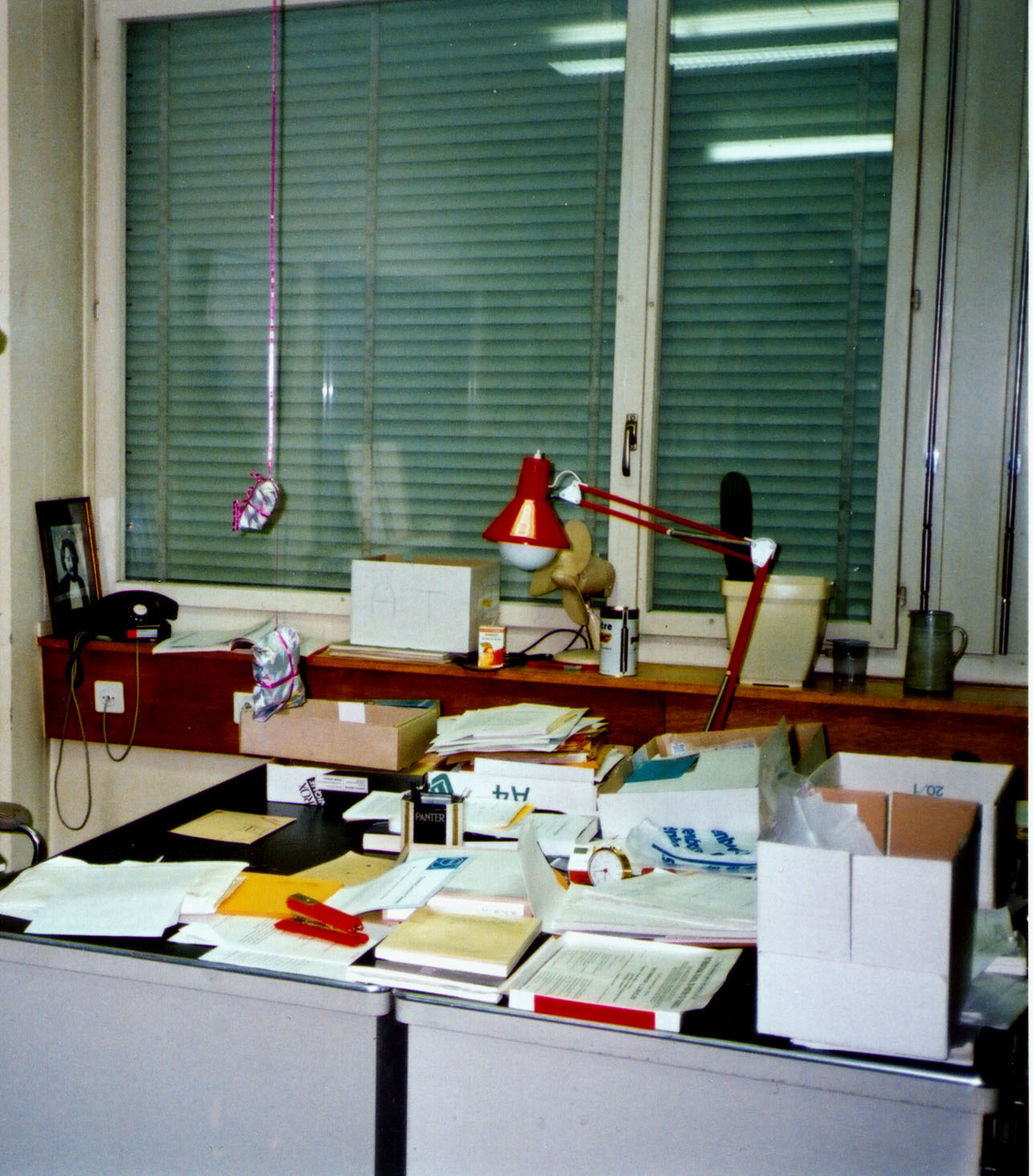
Figure 1: Desk of J.S. Bell at CERN

So you can imagine how exciting it was for me to get into contact with this man. I remember very well it was after a Seminar in the Theory Division, we had tea in the Common Room. There he approached me, the newcomer, and introduced himself: “I am John Bell, where are you from? What are you working on here?” My interest was calculating the properties of heavy quark-antiquark systems – quarkonium – specifically the wavefunctions, a hot subject at that time since charmonium (the $J/\psi$ family) had been found in 1974 and the even heavier system bottonium (the $\Upsilon$ family) recently discovered in 1977.

Bell was very interested in my explanations, he even liked my results, since they were in accordance with his Thomas-Fermi model calculations. So our discussions in this field began and became rather quickly a closer investigation into what is called duality.

2 Duality in hadronic reactions

The conception of duality is often used in physics. What I mean is that two seemingly different phenomena are strongly correlated to each other; they appear as the dual aspects of one and the same reality [1].

Hadron production in $e^{+}e^{-}$ collisions

Let us consider the production of hadrons (strongly interacting particles) in electron-positron collisions. Then among the hadrons there are also resonances produced, the $\rho,\phi,J/\psi,\Upsilon$ families of particles

$$e^{+}\;e^{-} \longrightarrow\;$$ hadrons (1)

$$\qquad\rho\;\qquad\quad\phi\;\;\;\quad J/\psi\;\quad\Upsilon\;\dots\qquad\textrm{resonances}$$

$$\qquad\Downarrow\quad\qquad\;\Downarrow\quad\quad\;\Downarrow\quad\quad\Downarrow$$

$$(u\bar{u}+d\bar{d})\quad\;(s\bar{s})\quad\;(c\bar{c})\quad(b\bar{b})\qquad\quad\textrm{boundstates}$$

The cross-section for these processes I have plotted qualitatively in Fig.2 and it exhibits the following feature. At low energies some pumps appear, the resonances, but at high energies the curve becomes quite flat or asymptotically smooth. These are two different phenomena, the resonance production and the asymptotic production of hadrons.

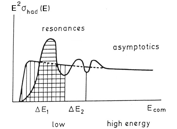
Figure 2: The hadronic cross-section in $e^{+}e^{-}$ collisions shown qualitatively

Question: Are they related to each other in a dual sense?

Answer: Yes, they are.

Question: How can we understand that?

Hadrons consist of quarks which are confined and interact strongly via gluons (the colour force). Now, at high energies, which corresponds to short distances, the quarks behave as quasi-free particles. The corresponding field theory – quantum chromo dynamics QCD – is asymptotically free. So there the process

$$e^{+}\;e^{-}\quad\longrightarrow\quad q\;\bar{q}\qquad\textrm{quasi-free (anti-) quark}$$ (2)

is a good approximation. Then the cross-section approaches a constant

$$E^{2}\sigma_{q\bar{q}}(E)\quad\longrightarrow\quad\frac{4\pi\alpha^{2}}{3}3\sum_{q}e_{q}^{2}\;=\;\textrm{constant}$$ (3)

which is proportional to the sum of the quark charges squared $e_{q}^{2}$ times the colour factor $3$. So we find the asymptotics correctly.

However, at low energies, where the quarks can penetrate into larger distances (the typical distance is of order fermi), they are confined and generate bound states which show up as resonances. These states are named quarkonium in analogy to positronium.

Duality

It was J.J. Sakurai [2] who formulated duality quantitatively. He found that if you average the cross-section suitably over all resonances then it agrees with the averaged asymptotics

$$\int_{\Delta E}E^{2}\sigma_{res}(E)dE = \int_{\Delta E}E^{2}\sigma_{q\bar{q}}(E)dE\;.$$ (4)

Relation (4) is called global duality.

Here is the point where Bell and I began our investigations [3].We simply asked: How far can we push duality?

How many resonances do we need in order to reproduce the asymptotics?

The answer is quite simple:

One individual resonance is enough!

This we called local duality [3]

$$\Delta E\quad\longrightarrow\quad\Delta E_{res}\;.$$ (5)

The explanation why it works we found in nonrelativistic potential theory.

3 Nonrelativistic potential theory

Although the bound states of quark-antiquark pairs are not ideal nonrelativistic systems, they decay and the relative velocity of the quarks is rather high ($v\approx 0.3\,c$), nonrelativistic potential theory is an amazingly powerful tool to describe their properties.

So for our purpose of energy averaging the cross-section we can approximate the resonances very well by a sum of delta functions

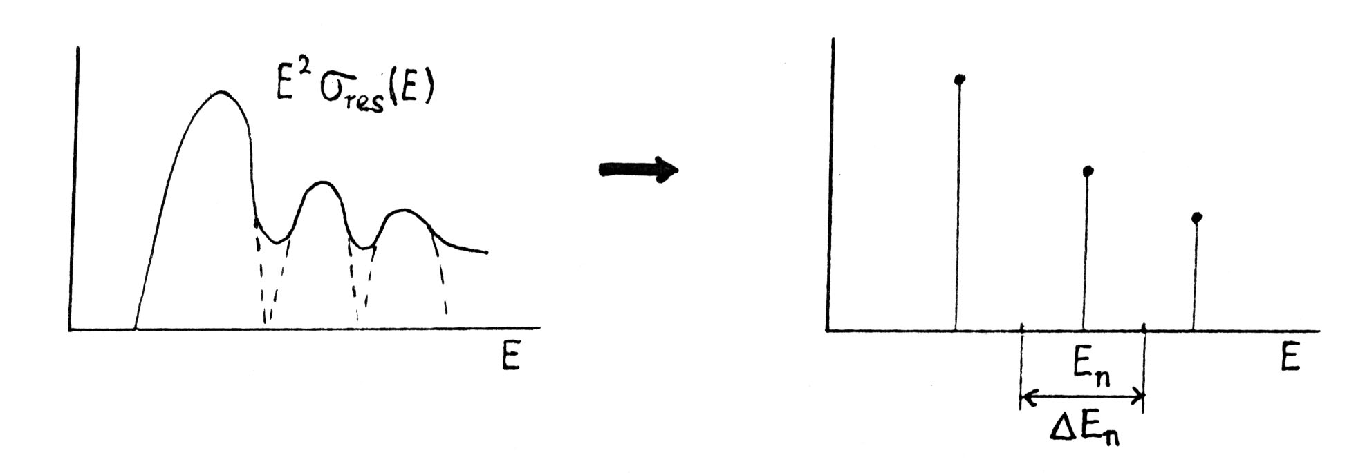
Figure 3: Approximation of resonances by delta functions

$$E^{2}\sigma_{res}(E) = 6\pi^{2}\sum_{n}\Gamma_{n}^{ee}\delta(E-E_{n})\;.$$ (6)

This replacement of the cross-section I have illustrated in Fig.3. The leptonic width of the resonance is related to the wave function at origin by

$$\Gamma_{n}^{ee} = N\frac{|\psi_{n}(0)|^{2}}{m^{2}}\qquad\qquad N=\frac{4\pi\alpha^{2}}{3}\cdot 3\cdot e_{q}^{2}\;.$$ (7)

On the other hand, in a nonrelativistic approximation the cross-section for quasi-free quarks depends just on their relative velocity $v=\sqrt{E/m}$

$$E^{2}\sigma_{q\bar{q}}(E) = N\frac{3v}{2}K(v)\;.$$ (8)

$$\hphantom{N\frac{3v}{2}}\Downarrow$$

Coulomb enhancement factor

The function $K(v)$ arises from the short distance part of the potential and is calculable. For example, in the case of the Coulomb potential it denotes the well-known Coulomb enhancement factor.

At this stage I must tell a story which happened when I was calculating some specific short distance functions $K(v)$. One day John Bell said: “Show me your calculations at home!” So in the evening I went to his apartment, in a big new building in Geneva, I took the lift to the second floor, and I was very excited when I rang the bell. John Bell opened the door, he was alone and offered me a drink, an orange juice. But I was so excited that I forgot to press my fingers on the glass, the whole orange juice dropped on the floor and polluted the beautiful carpet. I was shocked but John smiled and said: “You sit down and think – I clean the floor”. I certainly couldn’t think, I nearly fainted.

Coming back to expressions (6) and (8), if we compare both we can check quantitatively whether duality (4) in its local form (5) is true. The result for local duality is

$$4\pi|\psi_{n}(0)|^{2}\;=\;\frac{m^{2}}{\pi}\int_{\Delta E_{n}}dE\;v(E)K(E)\;,$$

$$\hphantom{4\pi|}\Uparrow\qquad\quad\hphantom{\frac{m^{2}}{\pi}\int_{\Delta E_{n}}dE\;v(}\Uparrow$$

o.k. within few % (9)

where we have chosen for each resonance the energy interval

$$\Delta E\quad\longrightarrow\quad\Delta E_{n}\;=\;\frac{E_{n}-E_{n-1}}{2}\;.$$ (10)

Calculating now the wavefunctions and the integrals in Eq.(3) explicitly it turns out that this local duality relation holds surprisingly well. For the ground state the duality integral in Eq.(3) approximates the wavefunction within a few percent, for the higher levels it practically coincides, and this rather independent of the potentials we used (for details see Ref.[3]).

Figure 4: Paper of magic moments

What’s the reason for it?

Let us further apply the mean value theorem to the duality integral in Eq.(3) then we find an expression which is quite familiar [4, 5, 6]. It’s the WKB relation

$$4\pi|\psi_{n}(0)|^{2} = \frac{m^{\frac{3}{2}}}{\pi}\sqrt{E_{n}}\;K(E_{n})\frac{dE_{n}}{dn}$$

wavefunction $$\Longleftrightarrow$$ energy spectrum (11)

which relates the wavefunction at origin to the energy spectrum. So we can trace back duality to a well-known result in quantum mechanics.

When we had our results and also thought to have understood them John proposed: “You begin to write the paper!” I felt very proud, worked all night, and showed him the paper the next day. John smiled: “Oh, that looks nice, I will have a closer look into it.” The day afterwards he returned the paper. I was shocked to find that there was no word left in the place where I had put it – it was a completely different paper! But, thank God, I slowly improved.

Résumé

Investigating local duality, the energy smearing of a resonance cross-section by a quasi-free quark cross-section, we find that relation (3) is very accurate independent of the considered potential.

This feature can be understood quite naively [1]. In the duality relation we allow for an energy spread, which means – via the uncertainty relation – that we focus on small values of the conjugate variable time. But for short times the corresponding wave cannot spread far enough to feel the details of the long distance part, the confining potential. So this part can be neglected, though certainly not the short distance part.

For this reason we can predict from a quasi-free $q\bar{q}$ pair the wave function at origin of the bound state, the leptonic width or the area of the resonance

$$\textrm{quasifree}\;q\bar{q}\quad\longrightarrow\quad|\psi_{n}(0)|^{2}\;\sim\;\Gamma_{res}^{ee}\;\sim\;\textrm{area of resonance}\;.$$ (12)

However, if we want to push the idea of duality even further in order to become sensitive for the position of the state, the mass of the resonance, then we penetrate into larger distances and we must have some information about confinement.

That’s the subject Bell and I got interested in next and it resulted in a wonderful collaboration which we called magic moments , see Fig.4.

4 Magic moments

One of John’s habits was to have a 4 o’clock tea . So in our afternoon discussions in John’s office we always made a break. It was like a ritual, at two minutes to four we left the office and stepped down to the CERN cafeteria. There John ordered in his typical British accent: “deux infusions verveine, s’il vous plâit”, John’s favorite tea. There, in a relaxed atmosphere, we talked not only about physics but also about politics, philosophy, and when Renata Bertlmann was with us we also had heated discussions about modern art.

When we worked at home a similar tea ritual took place in his flat, and as you can see from Fig.5, it took us quite a time to choose the right sort of verveine.

Figure 5: John Bell and Reinhold Bertlmann choosing the right sort of tea

So it was in this atmosphere verveine that John and I discussed how to include confinement in our duality idea in order to determine a bound state position.

Our starting point was the vacuum polarization tensor in quantum field theory. This is the Fourier transform of the vacuum expectation value of the time ordered product of two currents

$$i\int dx\;e^{iqx}\langle\Omega|T\;j_{\mu}(x)j_{\nu}(0)|\Omega\rangle = \Pi(q^{2})(q_{\mu}q_{\nu}-q^{2}g_{\mu\nu})\;.$$ (13)

It can be calculated within field theory, QCD, with help of Feynman diagrams, loop diagrams which I have depicted in Fig.6.

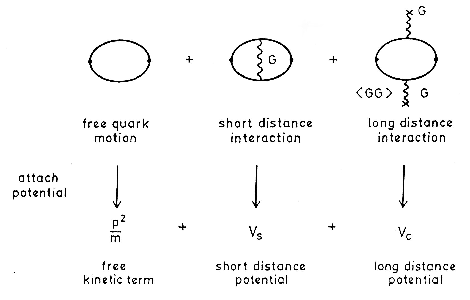
Figure 6: Feynman diagrams for the vacuum polarization tensor

The novel thing is that the usual perturbation series, representing the short distance interaction, gets modified by adding a small part (third diagram in Fig.6), the so-called gluon condensate $\langle GG\rangle$, the vacuum expectation value of two gluon field strength tensors. This part had been introduced at that time by a Russian group [7] in order to account for the longer distances, the influence of confinement.

Moments

Again, our investigation was within potential theory, where we could calculate both the perturbative and the exact result. For the energy smearing we chose exponentials (they worked best) and we defined the following nonrelativistic moment [8]

$$M(\tau) = \int dE\;e^{-E\tau}\;Im\Pi(E)\;,$$ (14)

where $Im\Pi(E)$ is the imaginary part of the vacuum polarization function calculable via the Feynman diagrams of Fig.6.

When we do the calculation, which is actually a perturbation theory calculation with respect to an imaginary time, the result is the following

$$M(\tau) = \frac{3}{8m^{2}}4\pi(\frac{m}{4\pi\tau})^{\frac{3}{2}}\biggl{\{}1+\frac{4}{3}\alpha_{S}\sqrt{\pi m}\;\tau^{\frac{1}{2}}-\frac{4\pi^{2}}{288m}\langle\frac{\alpha_{S}}{\pi}GG\rangle\;\tau^{3}\biggr{\}}\;.$$ (15)

The leading term corresponds to the free motion of the quarks (first diagram in Fig.6); it is perturbed by the $\alpha_{s}$ term, representing the short distance interaction (second diagram), and by the gluon condensate $\langle GG\rangle$ term, responsible for the longer distances (third diagram).

On the other hand, the exact moment – which is our ‘experimental’ moment containing the resonances, the bound states – is given by the optical theorem

$$Im\Pi(E)\;\sim\;\sigma(E)$$ (16)

which relates the imaginary part of the vacuum polarization function (the forward scattering amplitude) to the total cross-section. Inserting this cross-section within our potential theory, Eq.(6) together with Eq.(7), we get

$$Im\Pi(E) = \frac{3}{8m}\sum_{n}4\pi|\psi_{n}(0)|^{2}\delta(E-E_{n})\;.$$ (17)

This is the expression we have to insert into Eq.(14) to find the exact nonrelativistic moment.

Ground state

How do we obtain the ground state level?

To find the ground state level $E_{1}\/$, the mass of the resonance $M=2m+E_{1}\/$, we finally work with a logarithmic derivative, the ratio of moments

$$R(\tau) = -\frac{d}{d\tau}logM(\tau)\;=\;\frac{\int dE\;E\;e^{-E\tau}Im\Pi(E)}{\int dE\;e^{-E\tau}Im\Pi(E)}\quad\stackrel{{\scriptstyle\tau\longrightarrow\infty}}{{\longrightarrow}}\quad E_{1}\;.$$ (18)

For large (imaginary) times $\tau$ the ratio of moments cuts off the contributions from the higher states and projects the ground state energy $E_{1}\/$.

In the corresponding theoretical – perturbative – expression we regard the minimum value, even though not occurring at infinity, as an approximation to $E_{1}$

$$min\mathcal{R}(\tau)\;=\;E_{1}\;,$$

$$\quad\Uparrow\qquad\qquad\quad\Uparrow$$

o.k. within few % (19)

where the theoretical ratio of moments is given by a very simple formula

$$R(\tau) = \frac{3}{2\tau}-\frac{2}{3}\alpha_{S}\sqrt{\pi m}\tau^{-\frac{1}{2}}+\frac{4\pi^{2}}{96m}\langle\frac{\alpha_{S}}{\pi}GG\rangle\;\tau^{2}\;.$$ (20)

The mass of the corresponding resonance is then $M=2m+minR(\tau)\/$.

What’s now the result?

Let me discuss a typical example, charmonium, with values $m=1.4GeV$, $\alpha_{s}=0.3$ and $\langle\frac{\alpha_{s}}{\pi}GG\rangle=0.02GeV^{4}$. I have plotted the ratio $R(\tau)$ in Fig.7. It shows the following typical features:

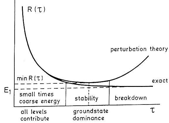
Figure 7: ratio of moments plotted qualitatively

The exact ratio approaches rather quickly its limit $E_{1}\/$. The theoretical ratio agrees perfectly for small times and stabilizes for large times. This stability, the minimum, happens to be already close to the ground state, quantitatively within $12\%$. So we get a good prediction for the position of the ground state.

Balance

We could show within potential theory that there exists a balance which we can phrase in the following way [8]:

$$\begin{array}[]{l}\textrm{course enough}\\ \textrm{pertubation theory o.k}\end{array}\qquad \Longleftrightarrow \qquad\begin{array}[]{l}\textrm{fine enough}\\ E_{1}\;\textrm{accurate}\end{array}$$ (25)

The energy average can be made coarse enough – involving small times – for the modified perturbation theory to work, while on the other hand fine enough for the individual levels to emerge clearly.

Surprising? Yes! Intuitively we had expected that for a clearly emerging level the confinement force must be dominant and not just a small additional perturbation. The moments, however, forced us to re-educate our intuition, when modifying the perturbation, levels do appear for magical reasons.

5 Equivalent potential

Since John and I worked within potential theory it was quite natural for us to ask whether one can attach a potential to this gluon condensate effect. This led us to our next collaboration [9, 10].

One of the nice things about being a physicist is that you travel around the world and meet your collaborators and friends everywhere. So it happened that in the year 1983 I stayed at the University of Marseille together with Eduardo de Rafael. He also invited John and Mary Bell to visit the institute. There we had interesting discussions and we also enjoyed the beautiful surroundings. One of our walks to the Calanque of Port Alon you can see in Fig.8. We even arranged a nice British weather for John, which was not so easy to get in the South of France.

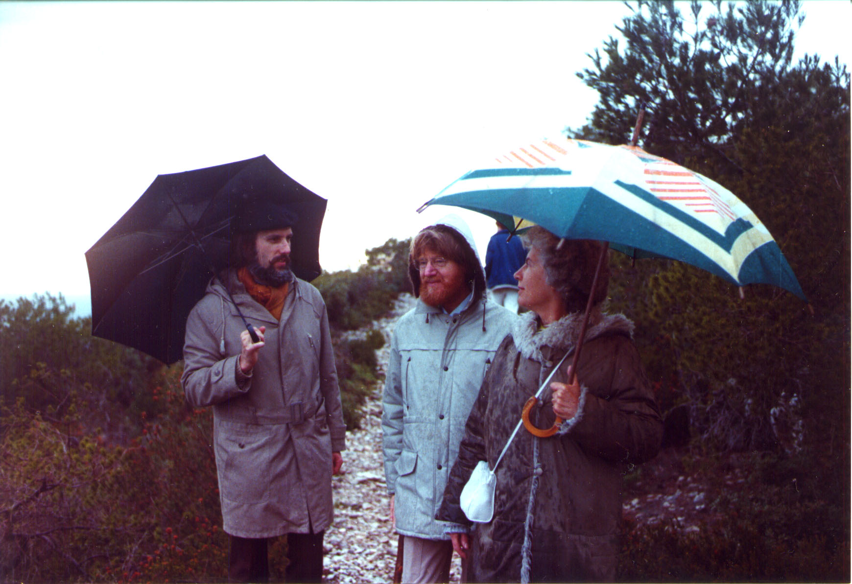
Figure 8: Reinhold Bertlmann, John Bell and Mary Bell on a walk in the Calanque of Port Alon, South of France, 1983

When starting from quantum field theory we faced the essential difficulty of representing the gluon condensate insertion, in the gluon propagator, by a potential. Whereas from the short distance part of the gluon propagator a potential can be extracted in the usual way, the familiar Coulomb potential, the long distance part, the gluon condensate contribution, diverges in this procedure. So we had to look for regularized quantities. But these we had already close at hand – these were our magic moments .

We know already the gluon condensate effect of quantum field theory in a nonrelativistic approximation, it is expression (15). So what we have to do is to calculate the nonrelativistic moment (14) within quantum mechanics determined by the Hamiltonian

$$H = \frac{p^{2}}{m}+V\;,$$ (26)

where $V$ represents now the potential.

The moment defined by equation (14) we can rewrite, by virtue of expression (17), as

$$M(\tau) = \int dE\;e^{-E\tau}Im\Pi(E)\;=\;\frac{3}{8m^{2}}\sum_{n}4\pi|\psi_{n}(0)|^{2}\;e^{-E_{n}\tau}$$ (27)

$$= \frac{3}{8m^{2}}\langle\vec{x}=0|e^{-H\tau}|\vec{x}=0\rangle$$

and we recover the (imaginary) time-dependent Green function at $\vec{x}=0\/$.

According to our previous procedure, we perturb the kinetic term by the potential with respect to the time $\tau$

$$e^{-H\tau} = e^{-\frac{p^{2}}{m}\tau}-\int_{0}^{\tau}d\tau^{\prime}\;e^{-\frac{p^{2}}{m}(\tau-\tau^{\prime})}\;V\;e^{-\frac{p^{2}}{m}\tau^{\prime}}\;.$$ (28)

The perturbation integral is determined by the potential and the familiar free Green function. For power potentials like

$$V = \sum_{s}\lambda_{s}r^{s}$$ (29)

the result for the moment is quite simple [8]

$$M(\tau) = \frac{3}{8m^{2}}4\pi(\frac{m}{4\pi\tau})^{\frac{3}{2}}\biggl{\{}1-\sum_{s}\lambda_{s}\Gamma(\frac{s}{2}+1)\;m\;(\frac{\tau}{m})^{\frac{s}{2}+1}\biggr{\}}\;.$$ (30)

This perturbation formula we have to compare with the corresponding field-theoretic expression (15). Identifying term by term ($s=-1$ and $s=4$) leads to the equivalent potential of Bell and Bertlmann [9]

$$V_{BB} = -\frac{4\alpha_{S}}{3r}+\frac{\pi^{2}}{144}\langle\frac{\alpha_{S}}{\pi}GG\rangle\;mr^{4}\;.$$ (31)

It is a superposition of Coulomb and quartic potential, it is quite steep and mass (or flavour) dependent. So it is rather different to those favoured by the potential modellers [11].

Finally, John and I also considered very heavy quarkonium systems which are very compact and dominated by the Coulomb interaction [12, 13]. There we also found a static potential reproducing precisely the gluon condensate contribution, however, it is also mass dependent [14].

In conclusion, no adequate bridge is found between field theory with a gluon condensate contribution, on the one hand, and popular potential models on the other. For an overview of this field I refer to Ref.[15].

6 Epilogue

John Bell was a deep and sharp thinker, a philosopher of Nature but with the tools of a theoretical physicist. And it was his great critical intellect that led him to his profound discoveries. So he found together with Roman Jackiw [16] the celebrated anomalies of quantum field theory , which opened the door to a deeper understanding of Nature (see Jackiw’s [17] contribution to the book), and which I could enjoy in discussing with John [18].

Bell’s famous dictum:

“Speakable and unspeakable in quantum mechanics”

which collects his quantum papers to a milestone book [19], or its variation Quantum [Un]speakables, the title of the conference commemorating John Bell [20], expresses truly his character. The use of words, their meaning, must be very precise. I could experience it in all our works.

Concern about terminology!

This was Bell’s demand. Like a moralist he attacked bad habits, the imprecise use of words. His attacks culminated in his brilliant article Against ‘measurement’ [21], where he branded the words that should be forbidden in any serious discussion:

“system, apparatus, environment, microscopic, macroscopic, reversible, irreversible, observable, information, measurement”.

For instance, observables should be replaced by his favorite concept, the beables [22], or measurements by experiments. But it is his great humor (for me his typical Irish wit) which makes his attacks so delightful. For example,

“ordinary quantum mechanics is just fine FAPP”

FAPP = for all practical purposes.

Bell’s wit you can find in all his actions, in every day life, and also when he communicated by drawing little sketches. In one sketch he characterized himself, and indeed, John was a gifted cartoonist. But before I show it I have to explain it a little bit.

In winter time, when it was cold, John liked to wear a Norwegian cap. On the cap one could see the letters: APPI LAPPI embroidered. Fig.9 shows the real cap.

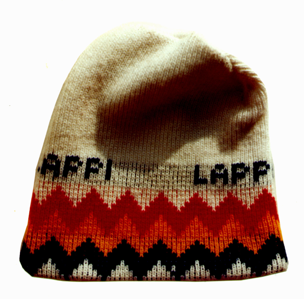
Figure 9: The real Norwegian APPI LAPPI cap of John Bell

With this APPI LAPPI cap on his head John has sketched himself – and as you can see from Fig.10,

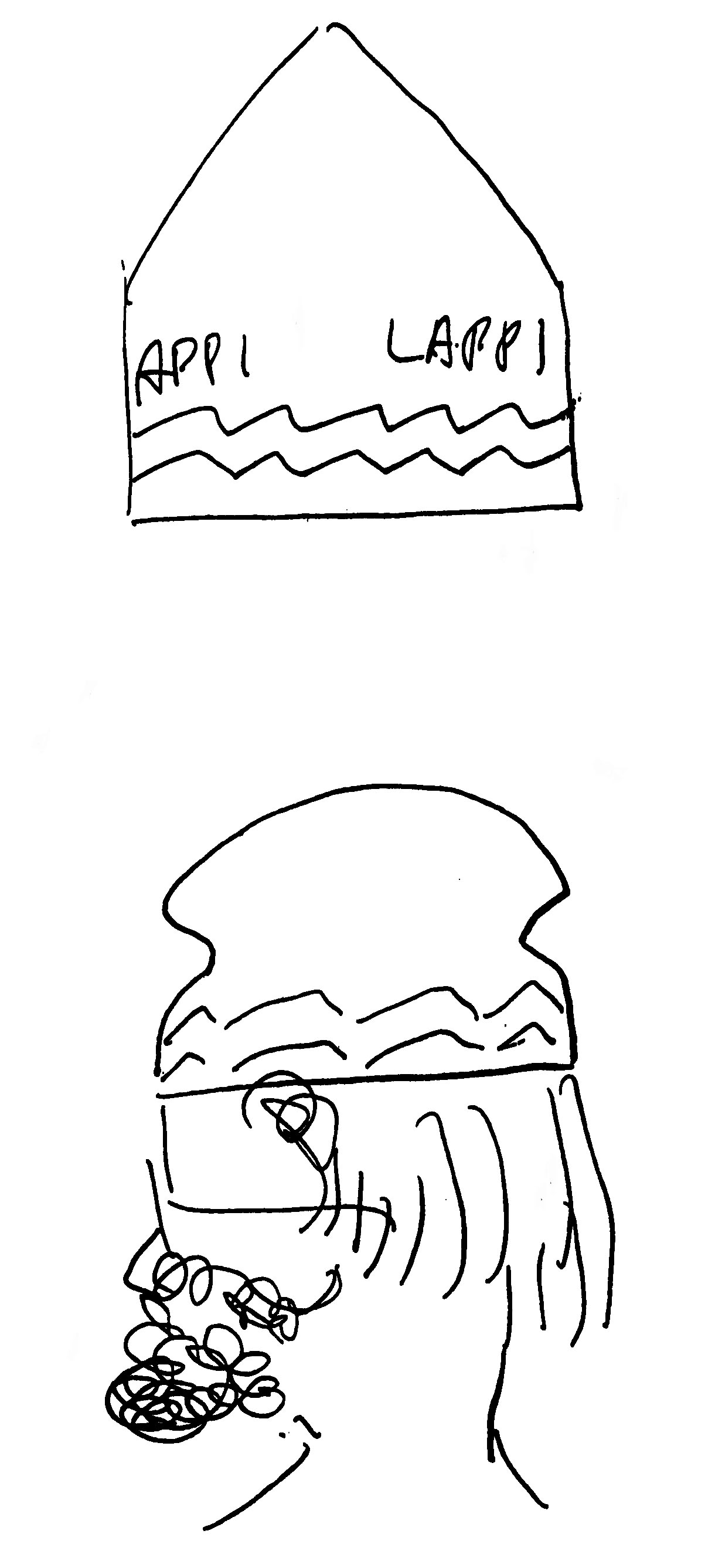
Figure 10: John Bell sketched by himself

the cap, the hairs, the glasses, the beard, his image is just perfect.

Now I come to the story some of you might know. Also I became a victim of his splendid wit. His article Bertlmann’s socks and the nature of reality [23], where he described the Einstein-Podolsky-Rosen correlations with Bertlmann’s socks, came out of the blue for me. In our first years of collaboration he never mentioned his quantum works to me. And I had not the slightest idea that he had noticed my habits of wearing socks of different colours (a habit I had had since my student days). Completely unexpected, this article appeared and pushed me instantaneously into the debate of quantum mechanics, and actually it was the cartoon, see Fig.11,

Figure 11: “Bertlmann’s socks”, sketch by John Bell

showing me with my odd socks in an EPR-like situation, which really changed my life. Everybody wants to see my socks now.

My answer to Bell’s article was also a paper which I named Bell’s theorem and the nature of reality and which I dedicated to him on occasion of his 60th birthday. So I wrote a preprint in July 1988 [24] and sent it to all universities, which was the customary procedure at that time. It appeared later on in Foundation of Physics [25]. In the Conclusion of the paper I took a little revenge by also drawing a cartoon, emphasizing the spooky action at a distance, see Fig.12.

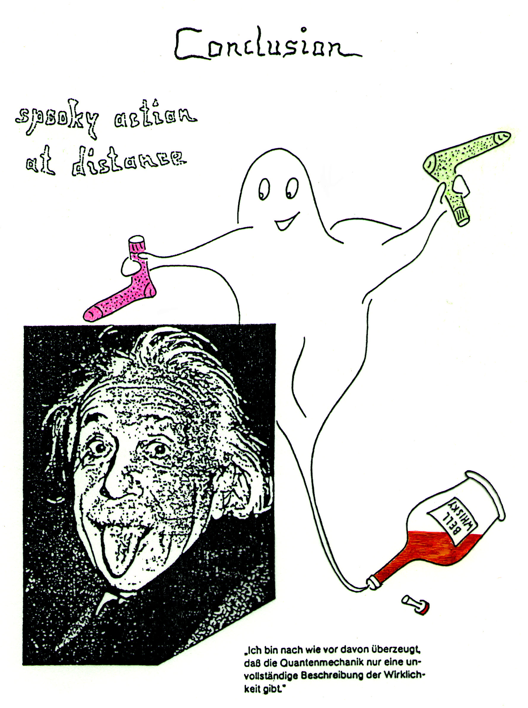
Figure 12: Conclusion of the preprint dedicated to John Bell

It amused John very much, who was rather unaccustomed to alcohol, that the spooky action escaped from a Bell whisky bottle which really does exist.

When I recall now my collaboration with John Bell and the time we spent together, I really can say it was a great and wonderful time, it was magic moments indeed, and I hope I have been able to give some impression of this in these pages.

References

- [1] R.A. Bertlmann, Acta Phys. Austr. 53 (1981) 305.
- [2] J.J. Sakurai, Phys. Lett. 46B (1973) 207.
- [3] J.S. Bell and R.A. Bertlmann, Z. Phys. C4 (1980) 11.
- [4] M. Krammer and P. Leal-Ferreira, Rev. Bras. Fis. 6 (1976) 7.
- [5] C. Quigg and J.L. Rosner, Phys. Rev. D17 (1978) 2364.
- [6] J.S. Bell and J. Pasupathy, Phys. Lett. 83B (1979) 389.
- [7] M.A. Shifman, V.I. Vainshtein and V.I. Zakharov, Nucl. Phys. B147 (1979) 385, 448, 519.
- [8] J.S. Bell and R.A. Bertlmann, Nucl. Phys. B177 (1981) 218.
- [9] J.S. Bell and R.A. Bertlmann, Nucl. Phys. B187 (1981) 285.
- [10] J.S. Bell and R.A. Bertlmann, Phys. Lett. 137B (1984) 107.
- [11] W. Lucha, F.F. Schöberl, D. Gromes, Phys. Rep. 200 (1991) 127.
- [12] H. Leutwyler, Phys. Lett. 98B (1981) 447.
- [13] M.B. Voloshin, Nucl. Phys. B154 (1979) 365.
- [14] R.A. Bertlmann and J.S. Bell, Nucl. Phys. B227 (1983) 435.
- [15] R.A. Bertlmann, Nucl. Phys. B (Proc. Suppl.) 23B (1991) 307.
- [16] J.S. Bell and R. Jackiw, Nuovo Cim. 60A (1969) 47.
- [17] R Jackiw, “John Bell’s observation on the chiral anomaly and some properties of its descendants”, hep-th/0011274.
- [18] R.A. Bertlmann, Anomalies in Quantum Field Theory. International series of monographs on physics 91, Clarendon Press, Oxford (1996).
- [19] J.S. Bell, Speakable and unspeakable in quantum mechanics, Cambridge University Press, (1987).
- [20] Quantum [Un]speakables, Conference in commemoration of John S. Bell, 10 - 14 November 2000, University of Vienna.
- [21] J.S. Bell, Physics World 3 (August 1990) 33.
- [22] J.S. Bell, “Beables for quantum field theory”, Article 19 of Ref.[19].
- [23] J.S. Bell, “Bertlmann’s socks and the nature of reality”, Article 16 of Ref.[19].
- [24] R.A. Bertlmann, “Bell’s theorem and the nature of reality”, Preprint University of Vienna, UWTh-Ph-1988-35, (1988).
- [25] R.A. Bertlmann, Found. Phys. 20 (1990) 1191.