Spatial magnetization profile in spherical nanomagnets with surface anisotropy: Green’s function approach

Abstract

We consider a single spherical nanomagnet and investigate the spatial magnetization profile $\mathbf{m}\left(\mathbf{r}\right)$ in the continuum approach, using the Green’s function formalism. The energy of the (many-spin) nanomagnet comprises an isotropic exchange interaction, a uniaxial anisotropy in the core and Néel’s surface anisotropy, and an external magnetic field. We derive a semi-analytical expression for the magnetization vector field $\mathbf{m}\left(\mathbf{r}\right)$ for an arbitrary position $\mathbf{r}$ within and on the boundary of the nanomagnet, as a solution of a homogeneous Helmholtz equation with inhomogeneous Neumann boundary conditions. In the absence of core anisotropy, we use the solution of this boundary problem and infer approximate analytical expressions for the components $m_{\alpha},\alpha=x,y,z$, as a function of the radial distance $r$ and the direction solid angle. Then, we study the effects of the nanomagnet’s size and surface anisotropy on the spatial behavior of the net magnetic moment.

In the presence of a core anisotropy, an approximate analytical solution is only available for a position $\mathbf{r}$ located on the surface,i.e. $\mathbf{r}=R\mathbf{n}$, where $R$ is the radius of the nanomagnet and $\mathbf{n}$ the verse of the normal to the surface. This solution yields the maximum spin deviation as a result of the competition between the uniaxial core anisotropy and Néel’s surface anisotropy. Along with these (semi-)analytical calculations, we have solved a system of coupled Landau-Lifshitz equations written for the atomic spins, and compared the results with the Green’s function approach.

For a plausible comparison with experiments, e.g. using the technique of small-angle magnetic neutron scattering, we have averaged over the direction solid angle and derived the spatial profile in terms of the distance $r$. We believe that the predictions of the present study could help to characterize and understand the effects of size and surface anisotropy on the magnetization configurations in nanomagnet assemblies such as arrays of well-spaced platelets.

• August 2023

1 Introduction

Why has studying nanoscaled systems suddenly become so important? How can a material that is so small be so influential as to trigger a tremendous research activity worldwide? To understand the power of nanomaterials, we need to understand how materials work at the very small scale. When the dimensions of the system are reduced down to the nanoscale, the first big change is the larger proportion of atoms at its surface, and this leads to a dramatic change in the chemical and physical properties. For example, bulk gold is an inert metal that does not react much and thus does not rust, whereas at the nanoscale, it works as a catalyst. A nanoparticle of gold about 90nm in size absorbs red and yellow light from the color spectrum, making the nanoparticle appear blue or green [1]. However, the same nanoparticle that is only 30nm in size, absorbs blue and green light, and so appears red. Today, we know that this is so because the optical properties of metal nanoparticles are dominated by the surface plasmon resonances for both absorption and scattering of light [2]. At the bottom end of the nanoscale, quantum phenomena start to emerge through a transition from the electronic-band structure to discrete energy levels [3]. This fundamentally alters the material properties and leads to many new phenomena [4], such as the energy gap and excitonic absorption of light, unique catalytic activity, and single-electron magnetism. In addition to the electronic structure alteration, the crystal structure also starts to exhibit significant changes with respect to the bulk material.

The reduction of the size and the entailed changes in the electronic and crystal structure fundamentally alter the magnetic properties as well. As the size reduces to the nanometer, the magnetic system, nowadays called a nanomagnet, exhibits a new phenomenon known as superparamagnetism [5, 6] with a change in the relevant temperature by an order of magnitude and in the relaxation time by several orders of magnitude. Furthermore, the large surface contribution in nanoscaled magnetic systems leads to inhomogeneous atomic-spin configurations [see Refs. [7, 8, 9, 10, 11] and references therein] and thereby to a drastically different behavior in response to external stimuli. For example, new modes of magnetization switching play a crucial role in many new spintronic applications [12]. Likewise, these surface-induced effects strongly affect the relaxation processes owing to a more complex potential energy and new excitation modes [13, 14].

Therefore, in order to understand and master the new magnetic properties of nano-elements, in view of efficient practical applications, it is essential to probe the novel features induced by their surfaces and interfaces. In particular, it is crucial to investigate the atomic-spin configurations within the nanomagnets and characterize the spatial profile of their magnetization. In this work, we present a study of the latter within spherical nanomagnets using the technique of Green’s functions (GF). This is part of a broader work that makes use of complementary techniques with the aim to better characterize surface-induced spin noncollineartities and their effects on the equilibrium and dynamic behaviors of assemblies of nanomagnets. In this context, the present work provides a general formalism that renders fairly precise and useful analytical expressions of the spatial magnetization profile, clearly presenting all the involved mathematical steps and approximations. As a byproduct, it confirms and elaborates on the conclusions reached by previous works regarding the effects of surface anisotropy in nanomagnets.

When averaged over the solid angle, the spatial magnetization profile may be compared with experiments, such as magnetic small-angle neutron scattering (SANS)[15] in assemblies of nanomagnets. Indeed, the present formalism constitutes a basis for computing the magnetic SANS cross-section of nanomagnets as a function of their various physical parameters. Accordingly, in a recent study [16, 17], we investigated the signature of surface-induced spin misalignments in the SANS cross section upon varying the applied magnetic field and the nanomagnet energy parameters.

Plan of the article: After an introduction, in Section 2, we present our model for a nanomagnet, viewed as a crystallite of $\mathcal{N}$ atomic magnetic moments and then describe the continuum approach for studying the spatial profile of its magnetization. In Section 3, we use the Green’s function technique to obtain the spin deviation vector in terms of surface anisotropy, in addition to other parameters, both with and without the anisotropy in the core. We plot the magnetization profile in the radial direction and study its behavior as we vary the size of the nanomagnet and the anisotropy constants. The results from the Green’s function formalism are also compared to the numerical calculations based on the solution of the system of coupled Landau-Lifshitz equations. Finally, in Section 4, we summarize the main results of this work and discuss the possibility of experimentally investigating the surface-induced spin-misalignments, e.g. by SANS technique. The paper ends with an Appendix.

2 Many-spin nanomagnet

2.1 Discrete lattice

A many-spin nanomagnet (NM) is viewed as a crystallite of $\mathcal{N}$ atomic magnetic moments $\mathbf{\mu}_{i}=\mu_{a}\mathbf{m}_{i}$ ($\left\|\mathbf{m}_{i}\right\|=1$) with $\mu_{a}=M_{s}v_{0}$, where $M_{s}$ is the saturation magnetization and $v_{0}$ is the volume of the unit cell of the underlying lattice. The magnetic state of the NM may be investigated with the help of the atomistic approach based on the anisotropic (classical) Dirac-Heisenberg Hamiltonian [18, 19, 20, 21, 22, 23, 7, 24, 25]

$$\mathcal{H} =-\frac{1}{2}\sum\limits_{\left\langle i,j\right\rangle}J_{ij}\,\mathbf{m}_{i}\cdot\mathbf{m}_{j}-\mu_{a}\mathbf{H}_{\rm{ext}}\cdot\sum_{i=1}^{\mathcal{N}}\mathbf{m}_{i}+\sum_{i=1}^{\mathcal{N}}\mathcal{H}_{{\rm an},i}$$

$$\equiv\mathcal{H}_{{\rm exc}}+\mathcal{H}_{{\rm Z}}+\mathcal{H}_{\rm an},$$

where $\mathcal{H}_{{\rm exc}}$ is the (nearest-neighbor) exchange energy, $\mathcal{H}_{{\rm Z}}$ the Zeeman contribution and $\mathcal{H}_{{\rm an}}\equiv\sum_{i=1}^{\mathcal{N}}\mathcal{H}_{{\rm an},i}$ the anisotropy energy with $\mathcal{H}_{{\rm an},i}=-K_{i}\,\mathcal{A}\left(\mathbf{m}_{i}\right)$, being the anisotropy contribution of each spin on site $i$; $\mathcal{A}\left(\mathbf{m}_{i}\right)$ is the anisotropy function that depends on the locus of the atomic spin $\mathbf{s}_{i}$. So, for core spins, the anisotropy may be uniaxial and/or cubic, while for surface spins there are a few models for on-site anisotropy that is very often taken as uniaxial with either a transverse or parallel easy axis. There is also the more plausible model proposed by Néel [26] for which $\mathcal{A}\left(\mathbf{m}_{i}\right)=\frac{1}{2}\sum\limits_{j=1}^{z_{i}}\left(\mathbf{m}_{i}\cdot\mathbf{u}_{ij}\right)^{2}$, where $z_{i}$ is the coordination number at site $i$ and $\mathbf{u}_{ij}$ a unit vector connecting the nearest neighbors $i,j$. The constant $K_{i}>0$ is usually denoted by $K_{{\rm c}}$ if the site $i$ is in the core and by $K_{{\rm s}}$ if it is on the boundary.

Therefore, in the sequel we will refer to the Néel Surface Anisotropy (NSA) model and this means that we consider a uniaxial anisotropy in the core with easy axis (whose verse is the unit vector $\mathbf{e}_{A}$) and Néel’s on-site anisotropy for spins on the surface. More precisely, in the NSA model we adopt the following anisotropy energy

$$\mathcal{H}_{{\rm an},i}=\left\{\begin{array}[]{lc}-K_{c}\left(\mathbf{m}_{i}\cdot\mathbf{e}_{A}\right)^{2},&i\in{\rm core}\\ \\ +\frac{1}{2}K_{s}{\displaystyle\sum_{j\in{\rm n.n.}}}\left(\mathbf{m}_{i}\cdot\mathbf{u}_{ij}\right)^{2},&i\in\mathrm{surface}.\end{array}\right.$$ (2)

The macroscopic state of the NM may be described using what is often called the superspin or macrospin, that is the net magnetic moment

$$\mathbf{m}=\frac{1}{\mathcal{N}}\sum_{i=1}^{\mathcal{N}}\mathbf{m}_{i}.$$ (3)

The dynamics of the magnetic moments $\mathbf{m}_{i}$ is governed by the (damped) Landau-Lifshitz equation (LLE) or, more precisely, the system of coupled Landau-Lifshitz equations written for the atomic magnetic moments $\mathbf{m}_{i}$ ($i=1,2,\ldots,\mathcal{N}$),

$$\frac{d\mathbf{m}_{i}}{d\tau}=\mathbf{m}_{i}\times\mathbf{h}_{{\rm eff},i}-\alpha\mathbf{m}_{i}\times\left(\mathbf{m}_{i}\times\mathbf{h}_{{\rm eff},i}\right),$$ (4)

with the (normalized) local effective field $\mathbf{h}_{{\rm eff},i}$, acting on $\mathbf{s}_{i}$, being defined by $\mathbf{h}_{{\rm eff},i}=-\delta\mathcal{H}/\delta\mathbf{s}_{i}$. $\tau$ is the reduced time given by $\tau=t/\tau_{{\rm s}},$ where $\tau_{{\rm s}}=\mu_{a}/\left(\gamma J\right)$ is a characteristic time of the system’s dynamics; $\gamma\simeq 1.76\times 10^{11}$ (Ts)^-1 is the gyromagnetic ratio and $\alpha$ the damping parameter ($\sim 0.01-0.1$). For example, for cobalt $J=8{\rm\ meV}$ and $\tau_{s}=70\ {\rm fs}$. In these units, $\mathbf{h}_{{\rm eff},i}=\mu_{a}\mathbf{H}_{{\rm eff},i}/J$, where $\mathbf{H}_{i}^{{\rm eff}}=-\left(1/\mu_{a}\right)\left(\delta\mathcal{H}/\delta\mathbf{m}_{i}\right)$ is the deterministic field that comprises the exchange field, the magnetic field $\mathbf{H}_{\mathrm{ext}}$ and the anisotropy field $\mathbf{H}_{A}$.

The spin configuration shown in Fig. 1, with the net magnetic moment along the diagonal, is obtained by (numerically) minimizing the energy (2.1) by solving the system of coupled Landau-Lifshitz equations (4) [23, 27, 28, 7, 29, 30]. This is a typical spin structure that is induced by the NSA in a spherical NM. Note that the atomic magnetic moments $\mathbf{m}_{i}$ progressively deviate from the global orientation (here the diagonal) as the site $i$ is located closer to the NM border and away from the diagonal.

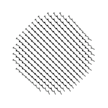
Figure 1: Magnetic structure of a spherical nanoparticle of linear size $N=20$, showing atoms in the plane $z=0$.

Orders of magnitude of materials parameters: Let us now give a few orders of magnitude of the physical parameters that appear in the Hamiltonian (2.1). First of all, we note that Eq. (2.1) is the energy per atom, obtained by dividing the total energy of the system by $\mathcal{N}$, the number of atoms in the NM. Hence, the physical parameters involved, namely $J,K$ and $\mu_{a}\left(\mu_{0}H\right)$, are measured in Joule per atom. For instance, the anisotropy energy, which is often written as $\tilde{K}V$ where $V$ is the volume of the NM and $\tilde{K}$ the density of anisotropy energy (in ${\rm J/m}^{3}$), becomes $\tilde{K}V=\mathcal{N}v_{0}\tilde{K}\equiv\mathcal{N}K$. Similarly, the Zeeman contribution which usually reads $\mu_{0}HM$ is now rewritten as $\mu_{0}HM=\mathcal{N}\mu_{a}\left(\mu_{0}H\right)$ . In the NSA model, we distinguish between the core (full coordination) and surface atoms (with smaller coordination). As such, the anisotropy constant $K_{c}$ applies only to atoms in the core of the NM and $K_{s}$ only to those on its surface. For instance, for cobalt, the magnetic moment per atom $\mu_{a}=n_{0}\mu_{B}$, with $n_{0}$ being the number of Bohr magnetons per atom ($n_{0}\simeq 1.7$) and $\mu_{B}=9.274\times 10^{-24}$J/T is the Bohr magneton. Hence, $\mu_{a}\simeq 1.58\times 10^{-23}\,{\rm J/T}$. Next, the magneto-crystalline anisotropy constant is roughly $K_{c}\simeq 3\times 10^{-24}$ J/atom, the surface anisotropy constant is around $K_{s}\simeq 5.22\times 10^{-23}\,$ Joule/atom and the (bulk) exchange coupling is $J\simeq 8\,\mathrm{mev}$ or $1.2834\times 10^{-21}$ J/atom. The lattice parameter is $a=0.3554$ nm. As such, $k_{c}\equiv K_{c}/J\simeq 0.00234$ while $k_{s}\equiv K_{s}/J\simeq 0.04$. The latter value is within the range of values estimated by several experimental studies. Indeed, one may find $K_{s}/J\simeq 0.1$ for cobalt [31], $K_{s}/J\simeq 0.06$ for iron [32], and $K_{s}/J\simeq 0.04$ for maghemite particles [33].

2.2 Continuum approach

In the continuum approach, the magnetic configuration of a system is described by the continuous magnetization vector field $\mathbf{M}\left(\mathbf{r}\right)$ constrained to a constant norm $M_{s}$. The relation between the discrete and continuous descriptions is [34]

$$\mathbf{M}\left(\mathbf{r}\right)=\sum_{i}\boldsymbol{\mu}_{i}/v_{0}$$ (5)

where $\boldsymbol{\mu}_{i}$ is the discrete magnetic moment of the $i^{\mathrm{th}}$ ion belonging to a given sub-lattice. The summation is carried over all sites in a physically small volume $v_{0}$, around a point whose position is $\mathbf{r}=(x,y,z)$, and within which the moments $\boldsymbol{\mu}_{i}$ are assumed to be uniform. The normalized magnetization density vector field is then defined by

$$\mathbf{m}(\mathbf{r})\equiv\mathbf{M}\left(\mathbf{r}\right)/M_{s}.$$ (6)

In the continuum limit, the exchange interaction is written in terms of the exchange stiffness $A$ (e.g. about $3.6\,{\rm pJ/m}$ for cobalt) as an integral over the volume $V$ of the NM

$$\mathcal{H}_{{\rm exc}} =A\int_{V}d\mathbf{r}\,\sum_{\alpha=x,y,z}\left(\mathbf{\nabla}m_{\alpha}\cdot\mathbf{\nabla}m_{\alpha}\right).$$ (7)

For a simple cubic lattice, we have the relation between $J$ and $A$: $A=J/2a$, with $a$ being the lattice constant. This is the classical analog of the relation that applies to a simple cubic lattice of quantum spins, $A=J\left\langle S^{2}\right\rangle/2a$.

Using the identity $\nabla\cdot(m_{\alpha}\cdot\nabla m_{\alpha})=m_{\alpha}\Delta m_{\alpha}+(\nabla m_{\alpha})^{2}$ and the divergence theorem, the exchange energy can split into a core and a surface contribution, namely

$$\mathcal{H}_{{\rm exc}} =-A\sum_{\alpha=x,y,z}\int_{V}m_{\alpha}\Delta m_{\alpha}\;\mathrm{d}^{3}r+A\sum_{\alpha=x,y,z}\oint_{\partial V}m_{\alpha}\nabla m_{\alpha}\;\mathbf{n}\,\mathrm{d}^{2}r.$$ (8)

Next, the Zeeman term reads,

$$\mathcal{H}_{{\rm Z}} =-M_{s}\mathbf{H}_{\mathrm{ext}}\cdot\int_{V}\mathrm{d}^{3}r\,\mathbf{m}\left(\mathbf{r}\right)$$ (9)

and the anisotropy energy for core spins becomes

$$\mathcal{H}_{{\rm core}} =-\frac{K_{c}}{v_{0}}\int_{V_{{\rm in}}}d^{3}r\,\left(\mathbf{m}\cdot\mathbf{e}_{z}\right)^{2}.$$

Note that $V_{{\rm in}}/v_{0}$, with $v_{0}=a^{3}$, is equal to the number of core atoms that we denote by $N_{{\rm c}}$, so that $V_{{\rm in}}K_{c}/v_{0}=N_{{\rm c}}K_{c}$. Regarding surface anisotropy, it was shown in Ref. [27] that the corresponding energy in the NSA model can be replaced by the approximate expression for a sphere [see Ref. [35] for a cube]

$$\mathcal{H}_{{\rm surface}}=-\frac{K_{s}}{2}\sum_{\alpha}\left|n_{\alpha}\right|m_{\alpha}^{2},$$ (10)

where $\mathbf{n}$ is the unit vector of the normal to the surface (the boundary $\partial V$ of the NM). Then, in the continuum limit, $\mathcal{H}_{{\rm surface}}$ becomes

$$\mathcal{H}_{{\rm surface}}=-\frac{K_{s}}{2a^{2}}\sum_{\alpha=x,y,z}\oint_{\partial V}d^{2}r\left|n_{\alpha}\right|m_{\alpha}^{2}.$$

Therefore, collecting all contributions, the nanomagnet’s Hamiltonian in Eq. (2.1) becomes in the continuum approach

$$\mathcal{H} =A\sum_{\alpha\in\{x,y,z\}}\left[\oint_{\partial V}m_{\alpha}\mathbf{\nabla}m_{\alpha}\cdot\mathbf{n}\,\mathrm{d}^{2}r-\int_{V}m_{\alpha}\Delta m_{\alpha}\;\mathrm{d}^{3}r\right]$$

$$-M_{s}\mathbf{H}_{\mathrm{ext}}\cdot\int_{V}d^{3}r\,\mathbf{m}\left(\mathbf{r}\right)$$

$$-\frac{K_{c}}{a^{3}}\int_{V}\left(\mathbf{m}\cdot\mathbf{e}_{A}\right)^{2}\;\mathrm{d}^{3}r-\frac{K_{s}}{2a^{2}}\sum_{\alpha\in\{x,y,z\}}\oint_{\partial V}\left|n_{\alpha}\right|m_{\alpha}^{2}\;\mathrm{d}^{2}r.$$

In the case of small spin-misalignment, where the magnetization density $\mathbf{m}\left(\mathbf{r}\right)$ slightly deviates from the homogeneous magnetization state $\mathbf{m}_{0}$ [see Fig. 1], a perturbation approach is applicable. Accordingly, $\mathbf{m}_{0}$ is considered as the principal unit vector associated with $\mathbf{m}(\mathbf{r})$ while the spin-misalignment is encoded in the vector field $\boldsymbol{\psi}\left(\mathbf{r}\right)$ with $\boldsymbol{\psi}\left(\mathbf{r}\right)\perp\mathbf{m}_{0}$. Therefore, we write [36, 37]

$$\mathbf{m}\left(\mathbf{r}\right)=\mathbf{m}_{0}\sqrt{1-\|\boldsymbol{\psi}\left(\mathbf{r}\right)\|^{2}}+\boldsymbol{\psi}\left(\mathbf{r}\right),$$ (12)

with $\mathbf{m}_{0}\cdot\mathbf{\boldsymbol{\psi}}=0$ and thereby $\left|\mathbf{m}\left(\mathbf{r}\right)\right|=1$, together with the condition (discussed later in the text)

$$\int_{V}d^{3}r\,\mathbf{\boldsymbol{\psi}}\left(\mathbf{r}\right)=0.$$ (13)

Assuming that $\psi_{\alpha}\ll 1,\alpha=x,y,z$, an approximate closed-form solution for the normalized magnetization density can be obtained by performing the second-order expansion of equation Eq. (12) with respect to $\boldsymbol{\psi}$ :

$$\mathbf{m}\left(\mathbf{r}\right)\cong\mathbf{m}_{0}+\boldsymbol{\psi}\left(\mathbf{r}\right)-\frac{1}{2}\|\boldsymbol{\psi}\left(\mathbf{r}\right)\|^{2}\mathbf{m}_{0}.$$ (14)

Next, one can rewrite the Hamiltonian (2.2) using a perturbation approach and minimizing with respect to the Cartesian components $\psi_{x},\psi_{y},\psi_{z}$, leading to a homogeneous (vector) Helmholtz equation for these components, together with inhomogeneous Neumann boundary conditions. However, owing to the transverse character of $\mathbf{\boldsymbol{\psi}}$ ($\mathbf{m}_{0}\cdot\mathbf{\boldsymbol{\psi}}=0$), it is more convenient to work in the local frame attached to $\mathbf{m}_{0}$, i.e. $\left(\mathbf{m}_{0},\mathbf{u}_{1},\mathbf{u}_{2}\right)$, where $\mathbf{u}_{1}$ and $\mathbf{u}_{2}$ are the following two unit vectors [37]

$$\mathbf{u}_{1} = \frac{\mathbf{m}_{0}\times\mathbf{e}_{A}}{\left\|\mathbf{m}_{0}\times\mathbf{e}_{A}\right\|},\quad\mathbf{u}_{2}=\frac{\mathbf{m}_{0}\left(\mathbf{m}_{0}\cdot\mathbf{e}_{A}\right)-\mathbf{e}_{A}}{\left\|\mathbf{m}_{0}\left(\mathbf{m}_{0}\cdot\mathbf{e}_{A}\right)-\mathbf{e}_{A}\right\|}.$$ (15)

In the new frame, we have

$$\mathbf{\boldsymbol{\psi}}=\psi_{1}\mathbf{u}_{1}+\psi_{2}\mathbf{u}_{2}$$ (16)

and $\|\boldsymbol{\psi}\left(\mathbf{r}\right)\|^{2}=\psi_{1}^{2}+\psi_{2}^{2}$. Consequently, with the help of a linear transformation, the problem is readily reduced to the following system of decoupled homogeneous scalar (dimensionless) Helmholtz equations

$$\left[\Delta_{\xi}-\kappa_{\beta}^{2}\right]\psi_{\beta}\left(\boldsymbol{\xi}\right)=0,\quad\beta=1,2$$ (17)

along with the inhomogeneous Neumann boundary conditions

$$\left.\frac{\mathrm{d}\psi_{\beta}}{\mathrm{d}\xi}\right|_{\xi=1}=\widetilde{k}_{s}\sum_{\alpha=x,y,z}\left|n_{\alpha}\right|\left(\mathbf{m}_{0}\cdot\mathbf{e}_{\alpha}\right)\left(\mathbf{u}_{\beta}\cdot\mathbf{e}_{\alpha}\right),\quad\beta=1,2.$$ (18)

Here we have introduced the dimensionless coordinates $\boldsymbol{\xi}=\mathbf{r}/R$, where $R$ is the NM radius, together with the following Helmholtz coefficients $\kappa_{\beta},\beta=1,2$, given by

$$\left\{\begin{array}[]{lll}\kappa_{1}^{2}&=&\left(\widetilde{\mathbf{h}}_{\mathrm{ext}}\cdot\mathbf{m}_{0}\right)+2\widetilde{k}_{c}\cdot\left(\mathbf{m}_{0}\cdot\mathbf{e}_{A}\right)^{2},\\ \\ \kappa_{2}^{2}&=&\left(\widetilde{\mathbf{h}}_{\mathrm{ext}}\cdot\mathbf{m}_{0}\right)+2\widetilde{k}_{c}\cdot\left[2\left(\mathbf{m}_{0}\cdot\mathbf{e}_{A}\right)^{2}-1\right].\end{array}\right.$$ (19)

where

$$\tilde{k}_{c}=\frac{1}{2}\left(\frac{D}{a}\right)^{2}k_{c},\qquad\tilde{k}_{s}=\left(\frac{D}{a}\right)k_{s},\qquad\tilde{h}_{\mathrm{ext}}=\frac{1}{2}\left(\frac{D}{a}\right)^{2}h_{\mathrm{ext}},$$ (20)

with $D=2R$ being the diameter of the NM, $k_{c}\equiv K_{c}/J$ and $k_{s}\equiv K_{s}/J$ the (dimensionless) reduced anisotropy constants introduced earlier, and $h_{\mathrm{ext}}\equiv\mu_{a}H_{\mathrm{ext}}/J$ the reduced magnetic field.

For later use and simplicity of notation, we introduce the surface anisotropy field

$$\Sigma_{\beta}\left(\mathbf{m}_{0},\mathbf{n}\right)\equiv\left.\frac{\mathrm{d}\psi_{\beta}}{\mathrm{d}\xi}\right|_{\xi=1}.$$ (21)

In the case of a core anisotropy easy axis in the $z$ direction, $\mathbf{e}_{A}=\mathbf{e}_{z}$,

$$\mathbf{u}_{1} = \frac{\mathbf{m}_{0}\times\mathbf{e}_{z}}{\sqrt{1-m_{0,z}^{2}}},\quad\mathbf{u}_{2}=\frac{\mathbf{m}_{0}\left(\mathbf{m}_{0}\cdot\mathbf{e}_{z}\right)-\mathbf{e}_{z}}{\sqrt{1-m_{0,z}^{2}}},$$ (22)

and

$$\Sigma_{1} =\widetilde{k}_{s}\frac{m_{0,x}m_{0,y}}{\sqrt{1-m_{0,z}^{2}}}\left(\left|n_{x}\right|-\left|n_{y}\right|\right),$$ (23)

$$\Sigma_{2} =\widetilde{k}_{s}\frac{m_{0,z}}{\sqrt{1-m_{0,z}^{2}}}\left[\left(\left|n_{x}\right|-\left|n_{z}\right|\right)m_{0,x}^{2}+\left(\left|n_{y}\right|-\left|n_{z}\right|\right)m_{0,y}^{2}\right].$$

3 Magnetization profile: Green’s function approach

To solve the homogeneous Helmholtz equation (17) for $\psi_{\beta}$, with the inhomogeneous Neumann boundary conditions (18), a specified gradient on the surface, we use the Green’s function (GF) approach [38, 39, 40]. The GF $\mathcal{G}_{\beta}\left(\boldsymbol{\xi},\boldsymbol{\xi}^{\prime}\right)$ for this problem satisfies the equation

$$\left[\Delta_{\xi}-\kappa_{\beta}^{2}\right]\mathcal{G}_{\beta}\left(\boldsymbol{\xi},\boldsymbol{\xi}^{\prime}\right)=-4\pi\delta\left(\boldsymbol{\xi}-\boldsymbol{\xi}^{\prime}\right),$$ (24)

and may be chosen to satisfy the homogeneous boundary condition of the same type as $\psi_{\beta}$, i.e. Neumann boundary conditions,

$$\left.\frac{\mathrm{d}\mathcal{G}_{\beta}}{\mathrm{d}\xi}\right|_{\boldsymbol{\xi}=1}=0.$$ (25)

In this case, we have the solution [40, 39, 27, 38]

$$\psi_{\beta}\left(\boldsymbol{\xi}\right)=\frac{1}{4\pi}\oint_{\partial V}d^{2}n^{\prime}\,\Sigma_{\beta}\left(\mathbf{m}_{0},\mathbf{n}^{\prime}\right)\mathcal{G}_{\beta}(\boldsymbol{\xi},\mathbf{n}^{\prime})$$ (26)

for $\boldsymbol{\xi}$ inside and on its boundary $\partial V$, where $\Sigma_{\beta}\left(\mathbf{m}_{0},\mathbf{n}\right)=\left.\frac{\mathrm{d}\psi_{\beta}}{\mathrm{d}\xi}\right|_{\boldsymbol{\xi}=\mathbf{n}}=\left(\mathbf{\nabla}_{\xi}\psi_{\beta}\right)\cdot\mathbf{n}$ is the outward normal gradient of $\psi_{\beta}$ at the surface of the NM, with $\mathbf{n}=\left(\sin\theta\cos\varphi,\sin\theta\sin\varphi,\cos\theta\right)$ and $d^{2}n=d\Omega=\sin\theta\,d\theta d\varphi$.

The result in Eq. (26) simply reflects the fact that the source of spin mis-alignment $\psi_{\beta}$ within the NM spin configuration is induced by surface anisotropy via the field $\Sigma_{\beta}=\left.\frac{\mathrm{d}\psi_{\beta}}{\mathrm{d}\xi}\right|_{\boldsymbol{\xi}=\mathbf{n}}$ given in Eq. (18). As discussed in Ref. [27], the spin mis-alignment (or disorder) initiated at the surface of the NM propagates into the body of the latter down to its center. In this case, the contribution of surface anisotropy to the overall anisotropy of the NM scales with its volume ($N^{3}$). In the presence of uniaxial anisotropy in the core, the surface spin disorder is screened out at a certain distance from the center and the contribution of the surface to the overall anisotropy then scales as the surface ($N^{2}$) [see Section 3.2 for further discussion].

3.1 No core anisotropy

In the absence of core anisotropy ($K_{{\rm c}}=0$) and magnetic field, $\kappa_{1}^{2}=\kappa_{2}^{2}=0$ [see Eq. (19)], the vector $\mathbf{m}_{0}$ is along the cube diagonal, i.e., $m_{0,\alpha}=1/\sqrt{3}$. Then, Eq. (17) reduces to the Laplace equation $\Delta\psi_{\beta}=0$, subjected again to the inhomogeneous Neumann boundary conditions (18). The corresponding GF $\mathcal{G}^{\left(0\right)}\left(\boldsymbol{\xi},\boldsymbol{\xi}^{\prime}\right)$ satisfies the Poisson equation

$$\Delta\mathcal{G}^{\left(0\right)}\left(\boldsymbol{\xi},\boldsymbol{\xi}^{\prime}\right) =-4\pi\delta\left(\boldsymbol{\xi}-\boldsymbol{\xi}^{\prime}\right).$$ (27)

However, integrating over the volume of the NM, we can see that the homogeneous boundary condition (25) can no longer be used. Instead, setting $\left.\frac{\mathrm{d}\mathcal{G}_{\beta}}{\mathrm{d}\xi}\right|_{\boldsymbol{\xi}=1}=C$, i.e. an inhomogeneous Neumann boundary condition, one finds that $C=-1$, and the GF function of the problem is then given by [27, 41] (up to a constant)

$$\mathcal{G}^{(0)}\left(\boldsymbol{\xi},\boldsymbol{\xi}^{\prime}\right) =\frac{1}{\left|\boldsymbol{\xi}-\boldsymbol{\xi}^{\prime}\right|}+\frac{1}{\sqrt{1+\mathbf{\xi}^{2}\mathbf{\xi}^{\prime 2}-2\left(\boldsymbol{\xi}\cdot\boldsymbol{\xi}^{\prime}\right)}}$$

$$\quad-\ln\left|1-\left(\boldsymbol{\xi}\cdot\boldsymbol{\xi}^{\prime}\right)+\sqrt{1+\mathbf{\xi}^{2}\mathbf{\xi}^{\prime 2}-2\left(\boldsymbol{\xi}\cdot\boldsymbol{\xi}^{\prime}\right)}\right|.$$

$$\left.\frac{\mathrm{d}\mathcal{G}^{(0)}}{\mathrm{d}\xi}\right|_{\xi=1} =-1.$$ (29)

When one of the arguments is on the surface, i.e. $\mathbf{\mathbf{\xi}}^{\prime}=\mathbf{n}^{\prime}$ ($\xi^{\prime}=1$), (3.1) simplifies into

$$\mathcal{G}^{(0)}\left(\boldsymbol{\xi},\mathbf{n}^{\prime}\right) =\frac{2}{\sqrt{1+\boldsymbol{\xi}^{2}-2\left(\boldsymbol{\xi}\cdot\mathbf{n}^{\prime}\right)}}$$

$$\quad-\ln\left|1-\left(\boldsymbol{\xi}\cdot\mathbf{n}^{\prime}\right)+\sqrt{1+\boldsymbol{\xi}^{2}-2\left(\boldsymbol{\xi}\cdot\mathbf{n}^{\prime}\right)}\right|.$$

Note that, in general, because of the inhomogeneous boundary condition (29), the GF $\mathcal{G}^{(0)}\left(\boldsymbol{\xi},\boldsymbol{\xi}^{\prime}\right)$ looses its symmetry of interchange $\boldsymbol{\xi}\longleftrightarrow\boldsymbol{\xi}^{\prime}$. However, by imposing the condition $\oint_{\partial V}\mathcal{G}^{(0)}(\boldsymbol{\xi},\mathbf{n}^{\prime})\,d^{2}n^{\prime}=0$, this symmetry is restored. The GF $\mathcal{G}^{(0)}\left(\boldsymbol{\xi},\boldsymbol{\xi}^{\prime}\right)$ in (3.1) yields $\left(1/4\pi\right)\oint_{\partial V}\mathcal{G}^{(0)}(\boldsymbol{\xi},\mathbf{n}^{\prime})\,d^{2}n^{\prime}=2-\ln 2$, and hence by making the replacement $\mathcal{G}^{(0)}\rightarrow\mathcal{G}^{(0)}-\left(2-\ln 2\right)$, which does not modify the boundary condition (29), we restore the symmetry $\boldsymbol{\xi}\longleftrightarrow\boldsymbol{\xi}^{\prime}$.

For $\xi\ll 1$ (or $r\ll R$), we obtain the fourth-order expansion

$$\mathcal{G}^{(0)}\left(\boldsymbol{\xi},\mathbf{n}\right) \simeq 2-\ln 2+3\left(\mathbf{n}\cdot\boldsymbol{\xi}\right)+\frac{5}{4}\left[3\left(\mathbf{n}\cdot\boldsymbol{\xi}\right)^{2}-\xi^{2}\right]$$

$$+\frac{7}{6}\left(\mathbf{n}\cdot\boldsymbol{\xi}\right)\left[5\left(\mathbf{n}\cdot\boldsymbol{\xi}\right)^{2}-3\xi^{2}\right]$$

$$+\frac{9}{32}\left[35\left(\mathbf{n}\cdot\boldsymbol{\xi}\right)^{4}-30\left(\mathbf{n}\cdot\boldsymbol{\xi}\right)^{2}\xi^{2}+3\xi^{4}\right]+\ldots$$

In this Section ($K_{{\rm c}}=0$), the spin deviation $\psi_{\beta}$ is then given by [40]

$$\psi_{\beta}^{\left(0\right)}\left(\boldsymbol{\xi}\right)=\frac{1}{4\pi}\oint_{\partial V}d^{2}n^{\prime}\,\Sigma_{\beta}\left(\mathbf{m}_{0},\mathbf{n}^{\prime}\right)\mathcal{G}^{\left(0\right)}\left(\boldsymbol{\xi},\mathbf{n}^{\prime}\right).$$ (32)

Note that had we kept the constant $2-\ln 2$ in $\mathcal{G}^{(0)}\left(\boldsymbol{\xi},\mathbf{n}\right)$, we would have obtained the same result since the contribution of this constant term vanishes under the surface integral when we substitute $\Sigma_{\beta}$ from Eqs. (21, 18). For the same reason, odd-order terms in the expansion (3.1) do not contribute to (32).

Therefore, using (18) and the expansion (3.1) up to $4^{\mathrm{nd}}$ order in $\xi$, we obtain the following explicit expressions ($\xi=r/R$) for the components of the spin deviation vector $\boldsymbol{\psi}^{\left(0\right)}$:

$$\psi_{1}^{\left(0\right)}\simeq\lambda_{s}\frac{m_{0,x}m_{0,y}}{\sqrt{1-m_{0,z}^{2}}}\left(\xi_{x}^{2}-\xi_{y}^{2}\right)\left[1+\frac{1}{16}\left(7\xi_{z}^{2}-\xi^{2}\right)\right],$$ (33)

$$\psi_{2}^{\left(0\right)}\simeq\lambda_{s}\frac{m_{0,z}}{\sqrt{1-m_{0,z}^{2}}}\left\{\begin{array}[]{l}m_{0,x}^{2}\left(\xi_{x}^{2}-\xi_{z}^{2}\right)+m_{0,y}^{2}\left(\xi_{y}^{2}-\xi_{z}^{2}\right)+\\ \frac{1}{16}\left[m_{0,x}^{2}\left(\xi_{x}^{2}-\xi_{z}^{2}\right)\left(7\xi_{y}^{2}-\xi^{2}\right)+m_{0,y}^{2}\left(\xi_{y}^{2}-\xi_{z}^{2}\right)\left(7\xi_{x}^{2}-\xi^{2}\right)\right]\end{array}\right\},$$ (36)

where $\lambda_{s}\equiv 15\widetilde{k}_{s}/32$. These expressions have been obtained using the following integrals

$$\frac{3}{4\pi}\oint_{\partial V}\left(\mathbf{n}\cdot\boldsymbol{\xi}\right)\left|n_{\alpha}\right|\;\mathrm{d}^{2}n=0,\quad\alpha=x,y,z,$$ (37)

$$\frac{1}{4\pi}\oint_{\partial V}\left[3\left(\mathbf{n}\cdot\boldsymbol{\xi}\right)^{2}-\xi^{2}\right]\left|n_{\alpha}\right|\;\mathrm{d}^{2}n=\frac{1}{8}\left(3\xi_{\alpha}^{2}-\xi^{2}\right),$$

$$\frac{1}{4\pi}\oint_{\partial V}\left[35\left(\mathbf{n}\cdot\boldsymbol{\xi}\right)^{4}-30\left(\mathbf{n}\cdot\boldsymbol{\xi}\right)^{2}\xi^{2}+3\xi^{4}\right]\left|n_{\alpha}\right|\;\mathrm{d}^{2}n=-\frac{1}{48}\left(35\xi_{\alpha}^{4}-30\xi^{2}\xi_{\alpha}^{2}+3\xi^{4}\right).$$

We see in Eq. (33) that the spin deviation $\mathbf{\boldsymbol{\psi}}^{\left(0\right)}$, caused by surface anisotropy, is linear in the corresponding constant $k_{s}$ (through $\lambda_{s}$) and depends on the equilibrium magnetic moment $\mathbf{m}_{0}$. It is also clear that this deviation depends on the position within the NM and on the direction along which $\xi$ is varied from the center out to the boundary of the NM. These results corroborate the discussion of the spin configuration shown in Fig. 1.

When $\mathbf{r}$ is on the surface, i.e. $\mathbf{\xi}=\mathbf{n}$, we obtain the largest deviation with respect to the homogeneous state $\mathbf{m}_{0}$ (using the $\xi^{2}$ expansion):

$$\psi_{1}^{\left(0\right)}\left(\mathbf{n},\mathbf{m}_{0}\right) \simeq\lambda_{s}\left(n_{x}^{2}-n_{y}^{2}\right)\frac{m_{0,x}m_{0,y}}{\sqrt{1-m_{0,z}^{2}}},$$ (38)

$$\psi_{2}^{\left(0\right)}\left(\mathbf{n},\mathbf{m}_{0}\right) \simeq\lambda_{s}\frac{m_{0,z}}{\sqrt{1-m_{0,z}^{2}}}\left[\left(n_{x}^{2}-n_{z}^{2}\right)m_{0,x}^{2}+\left(n_{y}^{2}-n_{z}^{2}\right)m_{0,y}^{2}\right].$$

As we will see below and in the next Section, it is handier in practice to use the expansions in Eq. (33) than the exact integral (32). For this purpose, we compare the two in Fig. 2.

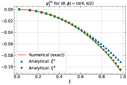
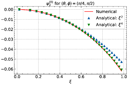
Figure 2: Components $\psi_{\alpha}^{(0)},\alpha=1,2$, of the spin deviation vector $\boldsymbol{\psi}$ as a function of (scaled) distance $\xi$ from the center of the nanomagnet. The red curve is a plot of the integral (32), numerically computed using the exact Green’s function (3.1). The blue and green curves (in symbols) are, respectively, obtained from Eq. (3.1) using the second and fourth order expansions. For both components, the direction of $\mathbf{\xi}$ is set to $\theta=\pi/4,\varphi=\pi/2$. $k_{c}=0,k_{s}=0.1$. [No magnetic field].

The plots in Fig. 2 show that the $4^{\mathrm{th}}-$order expansion of the Green function (3.1) renders a fairly good approximation to the components of $\boldsymbol{\psi}$ for all $\xi$ between $0$ and $1$, i.e. from the center of the nanomagnet up to its border.

We have also compared these results, rendered by the Green’s function technique, to the solution of the same boundary problem using the technique of spherical harmonics (SH), presented in Refs. [16, 17]. The outcome of this comparison is shown in Fig. 3 for two values of $k_{s}$. Note that here we have averaged the net magnetic moment over the direction solid angle [see discussion below]. We see that the $4^{\mathrm{th}}-$order approximation given in Eq. (3.1) and adopted here for the Green’s function $\mathcal{G}^{(0)}\left(\mathbf{n},\boldsymbol{\xi}^{\prime}\right)$, agrees very well with the expansion in terms of spherical harmonics up to the same order, to the $6^{\mathrm{th}}$ and even to the $10^{\mathrm{th}}$ order (not shown).

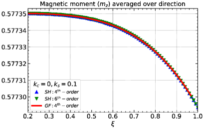
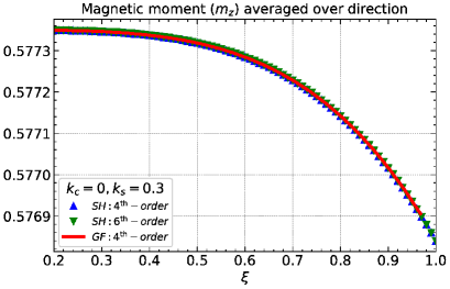
Figure 3: Component of the net magnetic moment, averaged over the solid angle, as a function of $\xi$, for $k_{c}=0,k_{s}=0.1$ (left) and $k_{c}=0.0,k_{s}=0.3$ (right), as given by the GF approach ($4^{\mathrm{th}}-$order) and SH approach ($4^{\mathrm{th}}$ and $6^{\mathrm{th}}$ orders). [No magnetic field].

Next, using (14), we can now write explicit expressions for the components of the NM magnetic moment, $m_{\alpha},\alpha=x,y,z$. In the frame $\left(\mathbf{m}_{0},\mathbf{u}_{1},\mathbf{u}_{2}\right)$ with $\mathbf{u}_{1}$ and $\mathbf{u}_{2}$ given in Eq. (22), we have

$$\boldsymbol{\psi}\left(\mathbf{r}\right)=\psi_{1}\mathbf{u}_{1}+\psi_{2}\mathbf{u}_{2}$$

or using $m_{0,\alpha}=1/\sqrt{3}$ and

$$\mathbf{u}_{1}\cdot\mathbf{e}_{x} =\frac{1}{\sqrt{2}},\mathbf{u}_{1}\cdot\mathbf{e}_{y}=\frac{-1}{\sqrt{2}},\mathbf{u}_{1}\cdot\mathbf{e}_{z}=0,$$

$$\mathbf{u}_{2}\cdot\mathbf{e}_{x} =\frac{1}{\sqrt{6}},\mathbf{u}_{2}\cdot\mathbf{e}_{y}=\frac{1}{\sqrt{6}},\mathbf{u}_{2}\cdot\mathbf{e}_{z}=-\sqrt{\frac{2}{3}},$$

we write $\boldsymbol{\psi}\left(\mathbf{r}\right)$ in the frame $\left(\mathbf{e}_{x},\mathbf{e}_{y},\mathbf{e}_{z}\right)$ as :

$$\boldsymbol{\psi}\left(\mathbf{r}\right) =\psi_{x}\mathbf{e}_{x}+\psi_{y}\mathbf{e}_{y}+\psi_{z}\mathbf{e}_{z}=\frac{1}{\sqrt{2}}\left(\begin{array}[]{l}\psi_{1}+\frac{1}{\sqrt{3}}\psi_{2}\\ -\psi_{1}+\frac{1}{\sqrt{3}}\psi_{2}\\ -\frac{2}{\sqrt{3}}\psi_{2}\end{array}\right).$$

Therefore, to $2^{\mathrm{nd}}$ order in $r$ (or $\xi$), we obtain the spatial profile of the net magnetic moment (for $k_{c}=0$)

$$\mathbf{m}\left(\mathbf{r}\right) \cong\mathbf{m}_{0}+\boldsymbol{\psi}\left(\mathbf{r}\right)=\left(\begin{array}[]{l}\frac{1}{\sqrt{3}}+\frac{1}{\sqrt{2}}\left(\psi_{1}^{\left(0\right)}+\frac{1}{\sqrt{3}}\psi_{2}^{\left(0\right)}\right)\\ \frac{1}{\sqrt{3}}+\frac{1}{\sqrt{2}}\left(-\psi_{1}^{\left(0\right)}+\frac{1}{\sqrt{3}}\psi_{2}^{\left(0\right)}\right)\\ \frac{1}{\sqrt{3}}\left(1-\sqrt{2}\psi_{2}^{\left(0\right)}\right)\end{array}\right)$$

with

$$\psi_{1}^{\left(0\right)} =\frac{\lambda_{s}}{R^{2}}\frac{1}{\sqrt{6}}\left(\tilde{\xi}_{x}^{2}-\tilde{\xi}_{y}^{2}\right)r^{2},$$

$$\psi_{2}^{\left(0\right)} =\frac{\lambda_{s}}{R^{2}}\frac{1}{3\sqrt{2}}\times\left[\left(\tilde{\xi}_{x}^{2}-\tilde{\xi}_{z}^{2}\right)+\left(\tilde{\xi}_{y}^{2}-\tilde{\xi}_{z}^{2}\right)\right]r^{2}$$

where $\tilde{\mathbf{\xi}}\equiv\mathbf{\xi}/\xi=\left(\sin\theta\cos\varphi,\sin\theta\sin\varphi,\cos\theta\right)$ gives the direction of $\mathbf{\xi}$ within the nanomagnet.

More explicitly, we have

$$\mathbf{m}\left(\xi,\theta,\varphi\right) \cong\mathbf{m}_{0}+\frac{\lambda_{s}}{3\sqrt{12}}\left(\begin{array}[]{l}\sin^{2}\theta\left(1+3\cos 2\varphi\right)-2\cos^{2}\theta\\ \sin^{2}\theta\left(1-3\cos 2\varphi\right)-2\cos^{2}\theta\\ -2\left(\sin^{2}\theta-2\cos^{2}\theta\right)\end{array}\right)\xi^{2}.$$ (44)

This analytical result, a quadratic expansion in $\xi$, may be compared to the numerical solution of the LLE (4). However, such a comparison is not easy in practice and here is why.

The magnetization profile similar to Eq. (44) has been obtained, in the discrete approach, by solving the (damped) LLE (4) for a spherical NM as defined earlier with the Hamiltonian in Eq. (2.1). More precisely, we prepare the NM by cutting a sphere in a simple-cubic $3D$ lattice of linear size $N=N_{x}=N_{y}=N_{z}$, the outcome being a sphere-shaped ensemble of $\mathcal{N}$ spins. Then, we set the physical parameters $J,K_{c},K_{s},h,$ etc, and run the Heun (or $4^{\mathrm{th}}$-order Runge-Kutta) routine to solve Eq. (4), until the equilibrium state is reached. The result is a spin configuration similar to that shown in Fig. 1. For each such a spin configuration, we collect the spatial profile of the net magnetic moment $\mathbf{m}$ as we go from the center to the border of the NM, in a given direction. Now, because of the discreteness of the underlying lattice (inside a spherical NM cut out of a simple-cubic lattice), the raw profile, or the components of $\mathbf{m}$ in Eq. (3) as a function of the lattice site $\mathbf{r}_{i}$, yields rather jagged plots. In order to smooth out the data, we may average over the direction $\left(\theta,\varphi\right)$ of $\mathbf{\xi}$ and consider only the radial profile of $\mathbf{m}$, i.e. $\mathbf{m}\left(\xi\right)$. This is given by

$$\left\langle\mathbf{m}\right\rangle_{\Omega}=\oint_{\partial V}\frac{d\Omega}{4\pi}\>\mathbf{m}\left(\boldsymbol{\xi}\right)=\mathbf{m}_{0}\times\left[1-\frac{1}{2}\oint_{\partial V}\frac{d\Omega}{4\pi}\|\boldsymbol{\psi}\left(\mathbf{r}\right)\|^{2}\right].$$ (45)

We see that upon averaging over the direction $\left(\theta,\varphi\right)$, the linear contribution in $\boldsymbol{\psi}$ vanishes. This can also be checked by performing the same average in Eq. (32) which, in turn, amounts to checking that the average of the GF (3.1) over the direction of $\mathbf{\xi}$ vanishes. This result is consistent with and justifies the condition (13).

Then, the integration over $\Omega$ yields

$$\oint_{\partial V}\frac{d\Omega}{4\pi}\left(\tilde{\xi}_{\alpha}^{2}-\tilde{\xi}_{\beta}^{2}\right)^{2}=\frac{4}{15},\quad\oint_{\partial V}\frac{d\Omega}{4\pi}\left(\tilde{\xi}_{x}^{2}-\tilde{\xi}_{z}^{2}\right)\left(\tilde{\xi}_{y}^{2}-\tilde{\xi}_{z}^{2}\right)=\frac{2}{15}$$

and upon using $1=\left(m_{0,z}^{2}+m_{0,x}^{2}+m_{0,y}^{2}\right)^{2}$, we obtain

$$\oint_{\partial V}\frac{d\Omega}{4\pi}\|\boldsymbol{\psi}\left(\mathbf{r}\right)\|^{2} =\frac{2}{15}\lambda_{s}^{2}\left(1-\sum_{\alpha}m_{0,\alpha}^{4}\right)\xi^{4}.$$ (46)

This finally leads to the solid-angle average of the magnetization profile

$$\left\langle\mathbf{m}\right\rangle_{\Omega}\left(\xi\right) \simeq\mathbf{m}_{0}\left[1-\frac{\lambda_{s}^{2}}{15}\left(1-\sum_{\alpha}m_{0,\alpha}^{4}\right)\xi^{4}\right].$$ (47)

Note that upon averaging over the direction $\left(\theta,\varphi\right)$, the quadratic contribution in Eq. (44) vanishes and only the quartic contribution remains in the expansion (14). The experimental techniques at our disposal today are not precise enough to allow for a probe of the magnetization profile in a given direction $\left(\theta,\varphi\right)$ within the nanomagnet. In addition, even if this were possible, the prototypical nanomagnet samples are assemblies with distributed nanomagnets and, as such only an average over the whole assembly can be accessed by measurements. This implies that if we were able to probe the magnetization profile, we should most likely observe the quartic behavior given by Eq. (47).

For later reference, we introduce the coefficient (of $\xi^{4}$)

$$\mathcal{C}_{\beta}\equiv m_{0,\beta}\frac{\lambda_{s}^{2}}{15}\left(1-\sum_{\alpha}m_{0,\alpha}^{4}\right),\quad\beta=x,y,z.$$ (48)

In order to further smooth out the lattice-induced jaggedness of the numerical data, we may also average over the magnitude of $\xi$ taken within slices (or ring bands) perpendicular to the radial direction. For this, we adopt an onion structure for the NM and plot the net magnetic moment $\left\langle\mathbf{m}\right\rangle_{\Omega}$ as a function of the points $\xi_{n},i=1\ldots M$, each of which being the center of a ring band. Doing so, leads to the discrete expression

$$\left\langle\mathbf{m}\right\rangle_{\Omega}^{n}\left(\xi_{n}\right) \simeq\mathbf{m}_{0}-\mathbf{m}_{0}\frac{\lambda_{s}^{2}}{15}\left(1-\sum_{\alpha}m_{0,\alpha}^{4}\right)\xi_{n}^{4}$$

or component-wise

$$\left\langle m_{\beta}\right\rangle_{\Omega}^{n}\left(\xi_{n}\right) \simeq m_{0,\beta}-\mathcal{C}_{\beta}\xi_{n}^{4}.$$ (49)

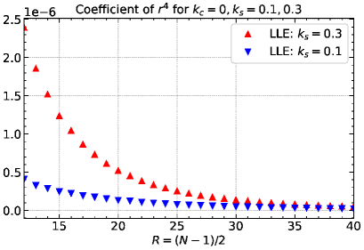
Figure 4: (Left) Magnetization profile $m_{z}$ against $\xi$ given by Eq. (49) and (right) coefficient of $r^{4}$ as a function of the NM radius $R=\left(N-1\right)/2$, with $N$ being the linear size. This is $\mathcal{C}_{z}$ defined in Eq. (48) divided by $R^{4}$. These results are for a spherical NM with $k_{c}=0,k_{s}=0.1,0.3$. [No magnetic field].

In the numerical calculations (numerical solution of the LLE), from each spin configuration obtained for a set of physical parameters and a given linear size $N$, we infer the average $\left\langle\mathbf{m}\right\rangle_{\Omega}^{n}\left(r_{n}=R\xi_{n}\right)$. The latter is fit to $a_{\beta}-\mathcal{C}_{\beta}r^{4}$, for $\beta=x,y,z$, to obtain the coefficient $\mathcal{C}_{\beta}$. The results are shown in Fig. 4 (right). It is clearly seen that a larger $k_{s}$ corresponds to a larger coefficient and thereby to stronger spin misalignments or deviations from $\mathbf{m}_{0}$. In addition, as the radius of the NM increases (we only show part of the data that have been obtained for $N=25,26,\ldots,111$ or $R=12,13,\ldots,55$), the coefficients for different values of $k_{s}$ tend to zero. Indeed, as the size increases, the ratio of the number of surface spins to the total number decreases to zero. This translates into negligible surface effects and thereby to vanishing spin deviations. Indeed, a fit of the curves in Fig. 4 (right) yields $\mathcal{C}_{\beta}\sim R^{-2}$, leading to $\left\langle m_{\beta}\right\rangle_{\Omega}^{n}\left(r\right)\sim a_{\beta}-\left(b_{\beta}/R^{2}\right)r^{4}$, where $b_{\beta}$ is a constant. This is illustrated in Fig. 5 where we compare the magnetic profile for different sizes to $m_{0,z}$, the magnetic moment in the uniform state. Finally, it is worth noting, by examining the vertical scale, that the deviation of the magnetic moment from the net direction $\mathbf{m}_{0}$ is rather small but it increases towards the NM boundary.

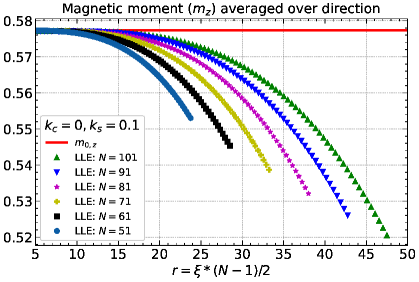
Figure 5: Spatial profile of the $z$ component of the NM net magnetic moment, averaged over the direction $\Omega$, as a function of the radial distance $r=\left(N-1\right)/2\times\xi$, with $0\leq\xi\leq 1$, for $k_{c}=0,k_{s}=0.1$. The continuous red line is the net magnetic moment component $m_{0,z}=1/\sqrt{3}$. On the scale used here, the GF function curve given by Eq. (49) coincides with the asymptotic straight line $m_{0,z}=1/\sqrt{3}$. [No magnetic field].

3.2 In the presence of core anisotropy

The more realistic situation with anisotropy in the core of the NM ($K_{{\rm c}}\neq 0$), as well as on the surface ($K_{{\rm s}}\neq 0$), is more involved. Indeed, there is no GF solving the problem stated in Eqs. (24, 25). However, since the coefficients $\kappa_{\alpha}^{2}$ in Eq. (19) are small, owing to the fact that the core anisotropy and the applied field are, in typical situations, small with respect to the exchange coupling, we can use a perturbative approach. Indeed, we may write [30]

$$\psi_{\beta}\left(\boldsymbol{\xi}\right)\simeq\psi_{\beta}^{\left(0\right)}\left(\boldsymbol{\xi}\right)+\kappa_{\beta}^{2}\,\psi_{\beta}^{\left(1\right)}\left(\boldsymbol{\xi}\right).$$ (50)

Then, substituting in Eq. (17), using $\Delta_{\xi}\psi_{\beta}^{\left(0\right)}\left(\boldsymbol{\xi}\right)=0$ [see Section 3.1] and dropping the term in $\kappa_{\beta}^{4}$, leads to

$$\Delta_{\xi}\psi_{\beta}^{\left(1\right)}\left(\boldsymbol{\xi}\right)=\psi_{\beta}^{\left(0\right)}\left(\boldsymbol{\xi}\right).$$

Next, we have

$$\left.\frac{\mathrm{d}\psi_{\beta}}{\mathrm{d}\xi}\right|_{\xi=1}=\left.\frac{\mathrm{d}\psi_{\beta}^{\left(0\right)}}{\mathrm{d}\xi}\right|_{\xi=1}+\kappa_{\beta}^{2}\,\left.\frac{\mathrm{d}\psi_{\beta}^{\left(1\right)}}{\mathrm{d}\xi}\right|_{\xi=1}.$$

Now, $\boldsymbol{\psi}^{\left(0\right)}$ is the major contribution to $\boldsymbol{\psi}$ that stems from surface anisotropy and $\boldsymbol{\psi}^{\left(1\right)}$ appears only in the presence of core anisotropy and/or applied magnetic field ($\kappa_{\beta}\neq 0$), which tend to reduce the spin misalignments. We may then consider that $\boldsymbol{\psi}^{\left(0\right)}$ still satisfies the boundary conditions (18), thus leading to

$$\left.\frac{\mathrm{d}\psi_{\beta}^{\left(1\right)}}{\mathrm{d}\xi}\right|_{\xi=1}=0.$$

Therefore, $\psi_{\beta}^{\left(1\right)}$ is a field that satisfies Poisson’s equation subjected to homogeneous Neumann boundary conditions, namely

$$\Delta_{\xi}\psi_{\beta}^{\left(1\right)}\left(\boldsymbol{\xi}\right) =\psi_{\beta}^{\left(0\right)}\left(\boldsymbol{\xi}\right),$$ (51)

$$\left.\frac{\mathrm{d}\psi_{\beta}^{\left(1\right)}}{\mathrm{d}\xi}\right|_{\xi=1} =0.$$ (52)

The solution of this problem can only exist if $\int_{V}d\boldsymbol{\xi}\,\psi_{\beta}^{\left(0\right)}\left(\boldsymbol{\xi}\right)=0$. It can be checked that this is indeed the case by using expressions (33). This is also compatible with the condition (13) that could be assumed to apply at all orders of perturbation. In this case, there exists a GF, call it $\tilde{\mathcal{G}}\left(\boldsymbol{\xi}^{\prime},\boldsymbol{\xi}\right)$, satisfying

$$\left\{\begin{array}[]{lll}\Delta_{\xi}\tilde{\mathcal{G}}\left(\boldsymbol{\xi}^{\prime},\boldsymbol{\xi}\right)&=&-4\pi\delta\left(\boldsymbol{\xi}-\boldsymbol{\xi}^{\prime}\right),\\ \\ \left.\frac{\mathrm{d}\tilde{\mathcal{G}}\left(\boldsymbol{\xi}^{\prime},\boldsymbol{\xi}\right)}{\mathrm{d}\xi}\right|_{\xi=1}&=&-1.\end{array}\right.$$ (53)

The solution of the problem then reads [40]

$$\psi_{\beta}^{\left(1\right)}\left(\boldsymbol{\xi}\right) =-\frac{1}{4\pi}\int_{V}d\boldsymbol{\xi}^{\prime}\,\tilde{\mathcal{G}}\left(\boldsymbol{\xi}^{\prime},\boldsymbol{\xi}\right)\psi_{\beta}^{\left(0\right)}\left(\boldsymbol{\xi}^{\prime}\right)-\frac{1}{4\pi}\oint_{\partial V}d^{2}n^{\prime}\,\psi_{\beta}^{\left(1\right)}\left(\mathbf{n}^{\prime}\right)\left.\frac{\mathrm{d}\tilde{\mathcal{G}}\left(\boldsymbol{\xi}^{\prime},\boldsymbol{\xi}\right)}{\mathrm{d}\xi^{\prime}}\right|_{\xi^{\prime}=1}$$

$$=-\frac{1}{4\pi}\int_{V}d\boldsymbol{\xi}^{\prime}\,\tilde{\mathcal{G}}\left(\boldsymbol{\xi}^{\prime},\boldsymbol{\xi}\right)\psi_{\beta}^{\left(0\right)}\left(\boldsymbol{\xi}^{\prime}\right)+D_{\beta},$$

where $D_{\beta}$ is a constant. In fact, we see that $\tilde{\mathcal{G}}\left(\boldsymbol{\xi},\boldsymbol{\xi}^{\prime}\right)$ is the solution of the same problem as $\mathcal{G}^{(0)}\left(\boldsymbol{\xi},\boldsymbol{\xi}^{\prime}\right)$ and, as such, we may simply take $\tilde{\mathcal{G}}\left(\boldsymbol{\xi},\boldsymbol{\xi}^{\prime}\right)=\mathcal{G}^{(0)}\left(\boldsymbol{\xi},\boldsymbol{\xi}^{\prime}\right)$. In addition, the constant $D_{\beta}$ can be determined by assuming that the spin mis-alignment vanishes at the center of the NM, i.e. $\psi_{\beta}^{\left(1\right)}\left(\boldsymbol{0}\right)=0$. This yields, using Eq. (3.1), $D_{\beta}=\frac{1}{4\pi}\int_{V}d\boldsymbol{\xi}\,\mathcal{G}^{(0)}\left(0,\boldsymbol{\xi}\right)\psi_{\beta}^{\left(0\right)}\left(\boldsymbol{\xi}\right)=0$.

Finally, we obtain the solution

$$\psi_{\beta}^{\left(1\right)}\left(\boldsymbol{\xi}\right) =-\frac{1}{4\pi}\int_{V}d\boldsymbol{\xi}^{\prime}\,\mathcal{G}^{(0)}\left(\boldsymbol{\xi},\boldsymbol{\xi}^{\prime}\right)\psi_{\beta}^{\left(0\right)}\left(\boldsymbol{\xi}^{\prime}\right).$$ (54)

Note that this result can also be obtained by proceeding through an expansion of the GF $\mathcal{G}_{\beta}\left(\boldsymbol{\xi},\mathbf{n}^{\prime}\right)$ that appears in Eq. (24), instead of the expansion in Eq. (50). This is done in A. Eq. (54), which derives from Eq. (51), suggests that $\psi_{\beta}^{\left(0\right)}$ acts as a source for the field $\psi_{\beta}^{\left(1\right)}$.

Let us now discuss the explicit calculation of the components $\psi_{\beta}^{\left(1\right)}\left(\boldsymbol{\xi}\right)$ of the spin deviation. Note that in Eq. (54), we have an integral over the volume and thereby none of the arguments of $\mathcal{G}^{(0)}\left(\boldsymbol{\xi},\boldsymbol{\xi}^{\prime}\right)$ is fixed on the surface. As a consequence, we have to use the exact expression (3.1), instead of the expansion (3.1). Unfortunately, it is then difficult to obtain a closed analytical result for the integral in Eq. (54). On the other hand, if we use instead the representation (54) in terms of the GF $\mathcal{G}^{(1)}$ in Eq. (59), we again encounter an integral over the volume of the product of two $\mathcal{G}^{(0)}$, one of which has both arguments inside $\partial V$. Consequently, we can provide analytical (approximate) expressions for $\psi_{\beta}^{\left(1\right)}\left(\boldsymbol{\xi}\right)$ only for $\boldsymbol{\xi}$ on the boundary $\partial V$. This should yield the largest contribution from $\psi_{\beta}^{\left(1\right)}\left(\boldsymbol{\xi}\right)$, as one obtains for $\psi_{\beta}^{\left(0\right)}$ in Eq. (38), see below. For arbitrary $\boldsymbol{\xi}$, with $0\leq\xi\leq 1$, we must resort to numerical integration.

For $\boldsymbol{\xi}$ on the boundary $\partial V$, i.e. $\boldsymbol{\xi}=\mathbf{n}$, we use Eqs. (3.1) and (38) to derive the following expressions for the components of $\boldsymbol{\psi}^{\left(1\right)}$ on the sphere:

$$\psi_{1}^{\left(1\right)}\left(\mathbf{n},\mathbf{m}_{0}\right) \simeq-\frac{\lambda_{s}}{14}\frac{m_{0,x}m_{0,y}}{\sqrt{1-m_{0,z}^{2}}}\left(n_{y}^{2}-n_{x}^{2}\right),$$ (55)

$$\psi_{2}^{\left(1\right)}\left(\mathbf{n},\mathbf{m}_{0}\right) \simeq-\frac{\lambda_{s}}{14}\frac{m_{0,z}}{\sqrt{1-m_{0,z}^{2}}}\left[\left(n_{x}^{2}-n_{z}^{2}\right)m_{0,x}^{2}+\left(n_{y}^{2}-n_{z}^{2}\right)m_{0,y}^{2}\right].$$

The components of the largest spin deviation represented by the (total) vector $\boldsymbol{\psi}$, within a spherical NM with equilibrium magnetic moment $\mathbf{m}_{0}$, are obtained by substituting (38) and (55) into Eq. (50). This yields

$$\psi_{1}\left(\mathbf{n},\mathbf{m}_{0}\right) \simeq\lambda_{s}\left(1-\frac{\kappa_{1}^{2}}{14}\right)\frac{m_{0,x}m_{0,y}}{\sqrt{1-m_{0,z}^{2}}}\left(n_{x}^{2}-n_{y}^{2}\right),$$ (56)

$$\psi_{2}\left(\mathbf{n},\mathbf{m}_{0}\right) \simeq\lambda_{s}\left(1-\frac{\kappa_{2}^{2}}{14}\right)\frac{m_{0,z}}{\sqrt{1-m_{0,z}^{2}}}\left[\left(n_{x}^{2}-n_{z}^{2}\right)m_{0,x}^{2}+\left(n_{y}^{2}-n_{z}^{2}\right)m_{0,y}^{2}\right].$$

Note that because of the factor $1-\kappa_{\alpha}^{2}/14$, these expressions are valid for $\kappa_{\alpha}\leq\sqrt{14}\simeq 3.74$. However, since they have been derived using an expansion in $\kappa_{\alpha}$, these expressions are actually valid for a much smaller $\kappa_{\alpha}$ and the previous condition adds no new constraint.

We can also numerically compute the integral in (54) and then average over the solid angle. However, although this procedure is quite affordable to today’s computers using optimized algorithms, it still remains rather costly with regard to the CPU resources, especially when several curves are needed for comparison. Here, we resort to the numerical solution of the LLE system, as done in the case of $k_{c}=0$, which allows for the full procedure in an easier manner. Accordingly, in Fig. 6 we plot the deviation of the $z$ component of the net magnetic moment, $\delta m_{z}\equiv m_{z}\left(r\right)-m_{z}\left(0\right)$, averaged over the direction $\Omega$, as a function of the radial distance $r=\left(N-1\right)/2\times\xi$, for $k_{s}=0.3$ and $k_{c}=0.01$ (full lines) and $k_{c}=0$ (dashed lines). We recall that the uniaxial anisotropy here is taken along the $z$ axis. If it is taken along the cube diagonal, the deviations will be much smaller. Indeed, we note that in the presence of anisotropy in the core with an easy axis in the $z$ direction, the state $\mathbf{m}_{0}$ is no longer along the cube diagonal; it is tilted towards the $z$ axis by an angle that depends on the relative strength of the core anisotropy ($k_{c}$). This results in a competition between the core and surface anisotropies.

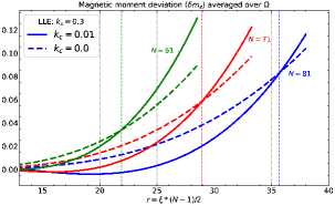
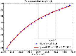
Figure 6: (Left) Deviation of the net magnetic moment $\delta m_{z}\equiv m_{z}\left(r\right)-m_{z}\left(0\right)$, averaged over the direction $\Omega$, as a function of the radial distance $r=\left(N-1\right)/2\times\xi$, for $k_{s}=0.3$ and $k_{c}=0.01$ (full lines) and $k_{c}=0$ (dashed lines). Note that, for the reasons explained in the text, the maximum value of $\xi$ is $0.95$ and this is why the curves do not reach the last points at $r=30,35,40$. (Right) The core correlation length over which the core anisotropy dominates (see text). [No magnetic field].

The results in Fig. 6 show that, both with and without core anisotropy, the overall spin deviations are reduced when the NM size increases. In addition, here we see that for a given size $N$ of the NM, the curves with and without core anisotropy (same color) intersect at a given distance $r_{c}$ from the center of the NM. As discussed earlier, the spin misalignments induced by the surface anisotropy tend to propagate from the boundary to the center of the NM, while the effect of the core (uniaxial) anisotropy is to align the spins parallel to each other and thus to push the spin misalignments out to the border. The competition between these two effects results in a critical radius $r_{c}$, or core correlation length (indicated by the dashed vertical lines), over which the core anisotropy dominates, thereby rendering a weaker spin deviation. This is illustrated by the fact that, for $r\leq r_{c}$, the continuous curves ($k_{c}\neq 0$) are below the dashed ones ($k_{c}=0$). Furthermore, in the plot on the right, we see that the distance $r_{c}$ increases with the radius $R=\left(N-1\right)/2$ of the NM ; it behaves as $a-b/R^{2}$ with $b>0$ (see the fitting curve in red). So, as $R$ increases the surface relative contribution decreases and the core anisotropy then dominates and pushes the spin noncollinearities farther out towards the NM border. As a consequence, the surface contribution to the overall anisotropy of the NM scales with the surface ($\sim R^{2}$), as was discussed in Ref. [27].

4 Summary, Conclusions, and Outlook

We have built a formalism for solving the Helmholtz equation, with inhomogeneous Neumann boundary conditions, satisfied by the spin deviation vector induced by surface anisotropy in a nanomagnet, using the technique of Green’s functions in the continuum limit. The nanomagnet has been modeled as a spherical crystallite of $\mathcal{N}$ atomic magnetic moments and whose energy comprises the exchange interaction, the Zeeman contribution and the anisotropy energy that discriminates between spins in the core, attributed a uniaxial anisotropy, and spins at the surface whose anisotropy is given by Néel’s model. We have also provided the numerical solution of a system of coupled Landau-Lifshitz equations written for the atomic magnetic moments and compared the results to those of the analytical approach. We have computed the solid-angle averaged components of the nanomagnet’s net moment as a function of the distance to the NM center in the radial direction, both in the absence and presence of anisotropy in the core. In the former case, we have provided good approximate analytical expressions for the spin deviation at an arbitrary position within the nanomagnet. In the latter case, however, the solution is only given numerically, either through a volume integral within the Green’s function approach, or numerically by solving the Landau-Lifshitz equations. Nonetheless, an analytical solution for this case has been given on the boundary of the NM, which represents the largest spin deviation. Both the numerical and (semi-)analytical results show that the spin deviations induced by surface anisotropy are stronger with larger surface anisotropy constant and/or smaller sizes.

As discussed in the introduction, the small-angle neutron scattering technique should provide us with a relatively precise probe of a signature of spin deviations in nanomagnets. However, with real samples, we are faced with various distributions (size, shape and anisotropy) and collective effects due to inter-particle interactions which may lead to a smearing out of the surface effects and the entailed sought-for spin misalignments. As a first step, we may consider doing measurements on an array of well separated platelets (or thin cylinders), thus avoiding strong inter-particle interactions while ensuring enhanced surface contributions to the overall anisotropy. In parallel to these investigations, further theoretical endeavor is required in order to take account of the inter-particle interactions together with other forms of anisotropy that might stem from different shapes and internal structures of the nanomagnets (e.g. platelets). In this context, the present Green’s function methodology may form the basis for computing the magnetic small angle neutron scattering cross-section of nanomagnets according to their magnetic materials parameters.

Appendix A Expansion of the Green’s function in the presence of core anisotropy

Similarly to the expansion of $\boldsymbol{\psi}$ in Eq. (50), we may write the GF $\mathcal{G}_{\beta}$ that appears in Eq. (24) as follows [30]

$$\mathcal{G}_{\alpha}\left(\mathbf{m}_{0},\boldsymbol{\xi},\boldsymbol{\xi}^{\prime}\right)=\mathcal{G}^{(0)}\left(\boldsymbol{\xi},\boldsymbol{\xi}^{\prime}\right)+\kappa_{\alpha}^{2}\,\left(\mathbf{m}_{0},\mathbf{h}\right)\mathcal{G}^{(1)}\left(\boldsymbol{\xi},\boldsymbol{\xi}^{\prime}\right)+\ldots.$$ (57)

It is then easy to see, upon using Eq. (27), that the correction term $\mathcal{G}^{(1)}\left(\boldsymbol{\xi},\boldsymbol{\xi}^{\prime}\right)$ satisfies the following equation (upon dropping terms in $\kappa_{\alpha}^{4}$)

$$\Delta\mathcal{G}^{(1)}\left(\boldsymbol{\xi},\boldsymbol{\xi}^{\prime}\right)\simeq\mathcal{G}^{(0)}\left(\boldsymbol{\xi},\boldsymbol{\xi}^{\prime}\right)$$ (58)

and that its solution can be written as a convolution

$$\mathcal{G}^{(1)}\left(\boldsymbol{\xi},\boldsymbol{\xi}^{\prime}\right)=-\frac{1}{4\pi}\int_{V}\mathcal{G}^{(0)}\left(\boldsymbol{\xi}^{\prime\prime},\boldsymbol{\xi}^{\prime}\right)\mathcal{G}^{(0)}\left(\boldsymbol{\xi},\boldsymbol{\xi}^{\prime\prime}\right)\;d^{3}\xi^{\prime\prime}$$ (59)

with the boundary condition [using Eq. (29)]

$$\left.\frac{\mathrm{d}\mathcal{G}^{(1)}}{\mathrm{d}\xi}\right|_{\xi=1} =\frac{1}{4\pi}\int_{V}\mathcal{G}^{(0)}\left(\boldsymbol{\xi}^{\prime\prime},\boldsymbol{\xi}^{\prime}\right)\;\mathrm{d}^{3}\xi^{\prime\prime}.$$ (60)

Then, in Eq. (26), we substitute the expansions for $\psi_{\beta}\left(\boldsymbol{\xi}\right)$ and $\mathcal{G}_{\beta}\left(\boldsymbol{\xi},\mathbf{n}^{\prime}\right)$, from Eqs. (50) and (57), respectively, and identifying the terms of the same order in $\kappa_{\beta}$, we obtain the following two equations

$$\psi_{\beta}^{\left(0\right)}\left(\boldsymbol{\xi}\right) =\frac{1}{4\pi}\oint_{\partial V}d^{2}n^{\prime}\left.\frac{\mathrm{d}\psi_{\beta}}{\mathrm{d}\xi}\right|_{\boldsymbol{\xi}=\mathbf{n}^{\prime}}\mathcal{G}^{(0)}\left(\boldsymbol{\xi},\mathbf{n}^{\prime}\right)$$

$$\psi_{\beta}^{\left(1\right)}\left(\boldsymbol{\xi}\right) =\frac{1}{4\pi}\oint_{\partial V}d^{2}n^{\prime}\left.\frac{\mathrm{d}\psi_{\beta}}{\mathrm{d}\xi}\right|_{\boldsymbol{\xi}=\mathbf{n}^{\prime}}\mathcal{G}^{(1)}\left(\boldsymbol{\xi},\mathbf{n}^{\prime}\right).$$

Next, using (52) we recover Eq. (32) for the component $\psi_{\beta}^{\left(0\right)}$ together with the following equation for $\psi_{\beta}^{\left(1\right)}$:

$$\psi_{\beta}^{\left(1\right)}\left(\boldsymbol{\xi}\right) =\frac{1}{4\pi}\oint_{\partial V}d^{2}n^{\prime}\Sigma_{\beta}\left(\mathbf{m}_{0},\mathbf{n}^{\prime}\right)\mathcal{G}^{(1)}\left(\boldsymbol{\xi},\mathbf{n}^{\prime}\right).$$ (61)

Then, replacing $\mathcal{G}^{(1)}\left(\boldsymbol{\xi},\mathbf{n}^{\prime}\right)$ by its expression in Eq. (59) leads to

$$\psi_{\beta}^{\left(1\right)}\left(\boldsymbol{\xi}\right)=-\frac{1}{4\pi}\int_{V}d^{3}\xi^{\prime\prime}\,\mathcal{G}^{(0)}\left(\boldsymbol{\xi},\boldsymbol{\xi}^{\prime\prime}\right)\left[\frac{1}{4\pi}\oint_{\partial V}d^{2}n^{\prime}\,\Sigma_{\beta}\left(\mathbf{m}_{0},\mathbf{n}^{\prime}\right)\mathcal{G}^{(0)}\left(\boldsymbol{\xi}^{\prime\prime},\mathbf{n}^{\prime}\right)\right].$$

Here, we recognize the term between brackets as $\psi_{\beta}^{\left(0\right)}$, according to Eq. (32), thus recovering (up to a constant) the result obtained in Eq. (54). Note that the main difference between the two representations, is that (54) is an integral over the volume of the NM whereas (61) is an integral over its surface.

References

- [1] D. R. Huffman C. F. Bohren. Absorption and scattering of light by small Nanoparticles. Willey-VCH Verlag GmbH, 1983.
- [2] Jin et al. Controlling anisotropic nanoparticle growth through plasmon excitation. Nature, 425:487–490, 2003.
- [3] Zhu et al. Correlating the crystal structure of a thiol-protected au25 cluster and optical properties. J. Am. Chem. Soc., 130:5883–5885, 2008.
- [4] Jin et al. Atomically precise colloidal metal nanoclusters and nanoparticles: fundamentals and opportunities. Chem. Rev., 116:10346–10413, 2016.
- [5] L. Néel, L’anisotropie superficielle des substances ferromagnétiques. Compt. Rend. Acad. Sci., 237:1468, 1953.
- [6] C. P. Bean and J. D. Livingston. Superparamagnetism. J. Appl. Phys., 30:S120, 1959.
- [7] H. Kachkachi and D.A. Garanin. Magnetic nanoparticles as many-spin systems. In D. Fiorani, editor, Surface effects in magnetic nanoparticles, page 75. Springer, Berlin, 2005.
- [8] G. Srajer, L. Lewis, S. Bader, A. Epstein, C. Fadley, E. Fullerton, A. Hoffmann, J. Kortright, K. M. Krishnan, S. Majetich, T. Rahman, C. Ross, M. Salamon, I. Schuller, T. Schulthess, and J. Sun. Advances in nanomagnetism via x-ray techniques. J. Magn. Magn. Mater., 307:1, 2006.
- [9] D.S. Schmool and H. Kachkachi. Chapter One - Collective Effects in Assemblies of Magnetic Nanaparticles. volume 67 of Solid State Physics, pages 1–101. Academic Press, 2016.
- [10] K. Koumpouras. Atomistic spin dynamics and relativistic effects in chiral anomagnets. Thesis/Dissertation, Uppsala University, 2017.
- [11] Òscar Iglesias and Hamid Kachkachi. Single Nanomagnet Behaviour: Surface and Finite-Size Effects, pages 3–38. Springer International Publishing, Cham, 2021.
- [12] Hirohata et al. Magnetic neutron scattering from spherical nanoparticles with néel surface anisotropy: analytical treatment. J. Magn. Magn. Mater., 509:166711, 2020.
- [13] P.-M. Déjardin, H. Kachkachi, Yu. Kalmykov, Thermal and surface anisotropy effects on the magnetization reversal of a nanocluster. J. Phys. D, 41:134004, 2008.
- [14] F. Vernay, Z. Sabsabi, and H. Kachkachi. ac susceptibility of an assembly of nanomagnets: Combined effects of surface anisotropy and dipolar interactions. Phys. Rev. B, 90:094416, Sep 2014.
- [15] Sebastian Mühlbauer, Dirk Honecker, Élio A. Périgo, Frank Bergner, Sabrina Disch, André Heinemann, Sergey Erokhin, Dmitry Berkov, Chris Leighton, Morten Ring Eskildsen, and Andreas Michels. Magnetic small-angle neutron scattering. Rev. Mod. Phys., 91:015004, Mar 2019.
- [16] M. P. Adams, A. Michels and H. Kachkachi. Magnetic neutron scattering from spherical nanoparticles with néel surface anisotropy: analytical treatment. J. Appl. Cryst., 55:1475–1487, 2022.
- [17] M. P. Adams, A. Michels and H. Kachkachi. Magnetic neutron scattering from spherical nanoparticles with néel surface anisotropy: atomistic simulations. J. Appl. Cryst., 55:1488–1499, 2022.
- [18] D.A. Dimitrov and Wysin, Effects of surface anisotropy on hysteresis in fine magnetic particles. Phys. Rev. B, 50:3077, 1994.
- [19] R.H. Kodama and A.E. Berkovitz, Atomic-scale magnetic modeling of oxide nanoparticles. Phys. Rev. B, 59:6321, 1999.
- [20] H. Kachkachi and D. A. Garanin. Boundary and finite-size effects in small magnetic systems. Physica A Statistical Mechanics and its Applications, 300:487–504, November 2001.
- [21] H. Kachkachi and D. A. Garanin. Spin-wave theory for finite classical magnets and superparamagnetic relation. European Physical Journal B, 22:291–300, August 2001.
- [22] O. Iglesias and A. Labarta, Finite-size and surface effects in maghemite nanoparticles: Monte Carlo simulations. Phys. Rev. B, 63:184416, 2001.
- [23] H. Kachkachi and M. Dimian, Hysteretic properties of a magnetic particle with strong surface anisotropy. Phys. Rev. B, 66:174419, 2002.
- [24] N. Kazantseva, D. Hinzke, U. Nowak, R. W. Chantrell, U. Atxitia, and O. Chubykalo-Fesenko, Towards multiscale modeling of magnetic materials: Simulations of FePt. Phys. Rev. B, 77:184428, 2008.
- [25] R. F. L. Evans, W. J. Fan, P. Chureemart, T. A. Ostler, M. O. A. Ellis, and R. W. Chantrell. Atomistic spin model simulations of magnetic nanomaterials. J. Phys.: Condens. Mat., 26:103202, 2014.
- [26] L. Néel, Anisotropie magnétique superficielle et surstructures d’orientation. J. Phys. Radium, 15:225, 1954.
- [27] D. A. Garanin and H. Kachkachi. Surface Contribution to the Anisotropy of Magnetic Nanoparticles. Phys. Rev. Lett., 90:065504, Feb 2003.
- [28] H. Kachkachi and H. Mahboub, Surface anisotropy in nanomagnets: Néel or Transverse? Surface anisotropy in nanomagnets: Néel or Transverse ? J. Magn. Magn. Mater., 278:334, 2004.
- [29] H. Kachkachi and E. Bonet, Surface-induced cubic anisotropy in nanomagnets. Phys. Rev. B, 73:224402, 2006.
- [30] H. Kachkachi, Effects of spin non-collinearities in magnetic nanoparticles. J. Magn. Magn. Mater., 316:248, 2007.
- [31] R. Skomski and J.M.D. Coey. Permanent Magnetism, Studies in Condensed Matter Physics Vol. 1. IOP Publishing, London, 1999.
- [32] K.B. Urquhart, B. Heinrich, J.F. Cochran, A.S. Arrott, and K. Myrtle, Ferromagnetic resonance in ultrahigh vacuum of bcc Fe(001) films grown on Ag(001). J. Appl. Phys., 64:5334, 1988.
- [33] R. Perzynski and Yu.L. Raikher. In D. Fiorani, editor, Surface effects in magnetic nanoparticles, page 141. Springer, Berlin, 2005.
- [34] E. A. Turov. Physical properties of magnetically ordered crystals. Academic Press, New York, 1965.
- [35] D. A. Garanin , Effective anisotropy due to the surface of magnetic nanoparticles. Phys. Rev. B, 98:2018, 2018.
- [36] A.M. Polyakov. Interaction of goldstone particles in two dimensions. applications to ferromagnets and massive yang-mills fields. Phys. Rev. B, 80:014420, 2009.
- [37] D. A. Garanin and H. Kachkachi, Magnetization reversal via internal spin waves in magnetic nanoparticles. Phys. Rev. B, 80:014420, 2009.
- [38] D. G. Duffy. Green’s functions with applications. Chapman and Hall/CRC, 2015.
- [39] P. M. Morse and H. Feshbach. American Journal of Physics, 22:410, 1954.
- [40] Ph. M. Morse and H. Feshbach. Methods of theoretical physics. McGraw-Hill, New York, 1953.
- [41] M. A. Sadybekov, B. T. Torebek, and B. Kh. Turmetov. Eurasian Math. J., 7:100, 2016.