Interpretable Deep Learning for Forecasting Online Advertising Costs: Insights from the Competitive Bidding Landscape

Abstract

As advertisers increasingly shift their budgets toward digital advertising, forecasting advertising costs is essential for making budget plans to optimize marketing campaign returns. In this paper, we perform a comprehensive study using a variety of time-series forecasting methods to predict daily average cost-per-click (CPC) in the online advertising market. We show that forecasting advertising costs would benefit from multivariate models using covariates from competitors’ CPC development identified through time-series clustering. We further interpret the results by analyzing feature importance and temporal attention. Finally, we show that our approach has several advantages over models that individual advertisers might build based solely on their collected data.

Introduction

The global advertising market has evolved beyond recognition over the past decades. According to Dentsu’s latest Global Ad Spend Forecast report, the total ad spend worldwide is expected to reach $738.5 billion in 2022, and digital advertising accounts for 55.5% of overall ad spend (Dentsu 2022). While continuing a remarkable recovery from the pandemic setbacks, digital advertising considerably drives sales growth through e-commerce platforms. The pandemic has disrupted shopping habits and led people to stay and/or work from home, resulting in a vast increase in online traffic. In response, advertisers spark a surge in investing in digital marketing channels driven by accelerated digital transformation. The ad agency Zenith predicts that ad budgets previously used to negotiate for shelf space in physical stores are increasingly shifted toward digital advertising in the post-pandemic era due to sustained demand from advertisers (Zenith 2022). Moreover, these advertisers have limited technical sophistication and marketing resources. They tend to collaborate with digital advertising networks such as Google and Facebook and adopt the auction mechanism to allow advertisers to bid on the keywords for paid search advertising. As such, the advertisers would benefit significantly from forecasting advertising cost in terms of cost-per-click (CPC) when making budget plans to estimate pay-per-click (PPC) marketing campaign returns.

Overall, the online advertising cost is dynamically determined by multiple factors, such as the industry, the quality of the ads, and the keywords, among others. According to Worldstream, the CPC in Google Ads vary significantly across sectors. The average CPC for the legal industry and consumer service reaches over $6, whereas the average CPC for E-commerce is only $1 (Irvine 2022). In particular, the advertising cost would highly depend on the macroeconomic condition and competitive landscape of the online advertising market, i.e., the CPC would depend on the competing advertiser’s bidding price at the time of auction. However, advertisers that only have access to their own budget plans may lack a holistic view of the bidding strategies of other advertisers. For example, Google Ads now provides a keyword planning tool for advertisers to evaluate their budget plans to forecast the future performance of marketing campaigns. But such an estimated CPC would only reflect the generic weekly average maximum CPC based on the different bidding strategies and would need to be adjusted to generate actual CPC. Additionally, the tool only displays the forecasted CPC, which limits the advertisers from gaining insights into the cost structure of the online advertising market.

Feature	Description	Type	Mean
adcustomerid	Advertiser unique id	identifier	-
category	Primary advertiser category	categorical	-
adcost	Daily actual advertising cost in USD	numerical	3,060.23
adclicks	Daily number of ad clicks	numerical	4,406.20
impressions	Daily number of ad impressions	numerical	71,775.81
cpc	Daily mean cost-per-click in USD (extracted as adcost/ adclicks)	numerical	1.11
adbudget	Monthly budget set by advertiser in USD (extracted from adcost)	numerical	3,053.33

Table 1: Features included in the final processed data frame used for modeling

To address this business question, we aim to forecast online advertising CPC for advertisers in different industries over multiple time horizons using a large-scale paid search dataset comprising many advertisers participating in the bidding competition. We do so by applying several off-the-shelf time-series forecasting techniques, including statistical methods (SARIMA), machine learning (XGBoost), and deep learning (LSTM and Transformer). For the models capable of handling covariates, we further introduce a set of additional features, including information about the advertisers and their competitors, and compare the multivariate performance to the one achieved by univariate time-series forecasting. We adopted three time-series clustering approaches, namely distance-based clustering, extracted-features-based clustering, and category-based clustering, respectively, to identify the relevant covariates within the expansive advertiser landscape. Our results show that the Temporal Fusion Transformer (TFT) based on recently developed Transformer architecture tends to outperform the other time-series forecasting methods. In particular, the TFT model that uses the covariates obtained from distance-based clustering achieves the best performance. Furthermore, we interpret the feature importance output by the TFT and demonstrate how our model learns the non-linear effect of budget levels on the CPC.

Importantly, this paper shows that advertisers would benefit from learning the competitive landscape in the Google Ads auction market, advertising strategies from similar advertisers. In our policy experiment, we test the learning stability of our proposed model during periods where significant economic crises are present in the training data. In doing so, we demonstrate the advantages over models that individual advertisers might build based solely on their collected data.

Data

Data Description

The data used in this research was provided by Grips, an e-commerce research platform based in Berlin, collecting adspend data through data partnerships worldwide. Data is collected directly through the first-party analytics tracking system, namely Google Analytics, and data partners allow Grips and other users of the ”give to share” model to analyze the data on an aggregated and anonymized level. Since the data is first-party, it is in the interest of each advertiser to be in the cleanest possible format. Furthermore, all data sources are structured identically, and no further tagging, classification, or normalization was necessary. The dataset encompasses over 249,000 advertisers, covers around 9.2% of the total Google Adrevenue and shows a correlation to Alphabet, Google’s parent company’s, reported adrevenue of more than 0.9. The dataset covers multiple ad distribution networks provided by Google Ads: Google Search, Search Partners, Content, and Cross-network. Data is available daily, offering device category and corresponding metrics: adcost, adclicks, and impressions.

Data Preprocessing

To cut down the significant data size and keep as many industries covered sufficiently, we opted for a geographical subset, i.e., choosing to analyze only advertisers in Germany. Furthermore, within this analysis, we are only focusing on Google’s paid search, as opposed to, e.g., Search Partners and Cross Networks. This should eliminate further actors within the dependency line as changes in other ad or website provider partners might have an unaccounted but heavy influence on ad success. In addition, paid search results will organically open up research opportunities on the keyword level in the future.

Advertisers generally set their marketing budget monthly. However, it is possible to adjust spending during the month, and Google algorithmically allocates the budget not at a constant level but at a highly fluctuating level from day to day. The competitive patterns we are looking for to support our predictions are also likely to occur at shorter intervals than the monthly budget inputs, as online price spikes and trends, together with customer and competitor responses, can change quickly. Therefore, we chose to aggregate and use data daily rather than monthly or weekly granularity to preserve as much detail as possible. This decision is also supported from a technical perspective, as deep learning models, which are a central part of our study, have shown to work best when fed with long time series consisting of many data points (Cerqueira, Torgo, and Soares 2019).

We use the last three years of available data to train our models on the closest representation of current advertising behavior. The COVID-19 pandemic has significantly impacted online pricing structures during our selected time frame. However, the target of our prediction is cost-per-click which is a relative measure of advertising cost and the number of clicks. Therefore, our study is not significantly affected by absolute cost changes occurring during the pandemic, allowing us to select the latest possible split date and provide the maximum amount of data for deep learning.

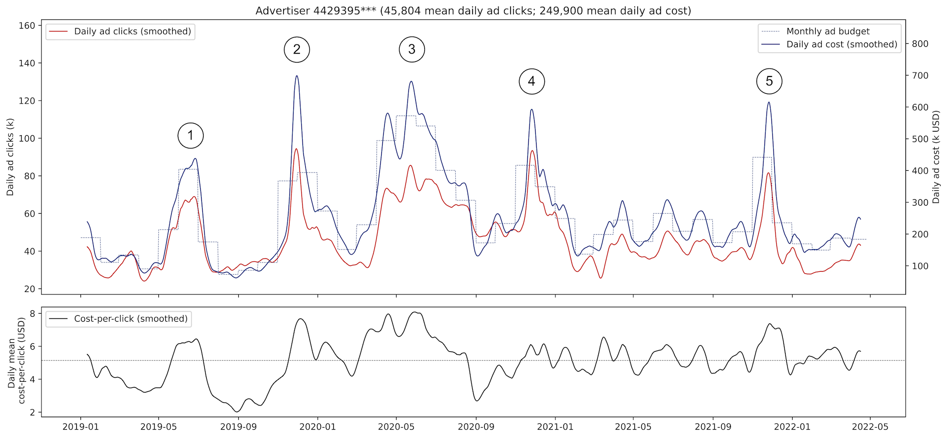
Figure 1: Simplified example of feature interconnections in Google online advertising over three years

Time series modeling generally requires clean data with no missing time steps for all models in the scope of our study. We consequently filter all advertisers that exceed more than one percent of missing data on our predefined daily aggregated level. All remaining missing time steps are imputed following a linear interpolation strategy, i.e., generating data points to connect the two closest observations available linearly. Table 1 summarizes the set of features from the dataset used for modeling. We further extract four temporal descriptives: day of the week, day of the year, month of the year, and a 7-day lag of the target, CPC, to support the modeling of weekly seasonalities and special days like Christmas.

Exploratory Data Analysis

Figure 1 demonstrates the logic of the key variables in online advertising. Understanding the interconnections between these factors is fundamental for building meaningful predictive models: Google Ads requires the advertiser to set a monthly budget indicating how much he is willing to spend on average per day (monthly ad budget) (Google 2022). Google then automatically allocates the budget to the individual auctions daily (actual daily ad cost). The allocation is thereby not constant across the days of the month, but most of the time series underlies a weekly seasonality that changes in amplitude (Yuan, Wang, and Zhao 2013).

Increasing the ad budget is to gain higher ranks in the bidding iterations and consequently generate more attention. Reliable measures for ad attention are how often the ad appeared on a user’s screen (daily ad impressions) and how often the user reacted to it by clicking the link (daily ad clicks). As shown by the example in Figure 1, the amount of clicks generated is highly influenced by the budget input. Across all advertisers in scope, clicks and impressions have a Pearson correlation coefficient to the monthly ad budget of 0.71 and 0.69, respectively.

The daily average cost-per-click is calculated as the dividend of the actual daily ad cost and the number of ad clicks on a given day. It indicates how effectively a campaign converts ad budget to user clicks – a higher CPC means less effective marketing. Our example shows that the CPC development cannot be explained solely by the abovementioned variables. Even though the budget increases, annotated in Figure 1, are roughly on the same level, the conversion to daily actual ad cost and the CPC does not follow proportionally. We take this as an indication that further drivers of online advertising effectiveness are located deeper in the corresponding data of multiple competing entities. This is supported by recent research showing that various online advertising-related factors impact the CPC and actual sales through online channels, where the significance of the variable dependencies varies over time (Yang et al. 2022).

Methodology

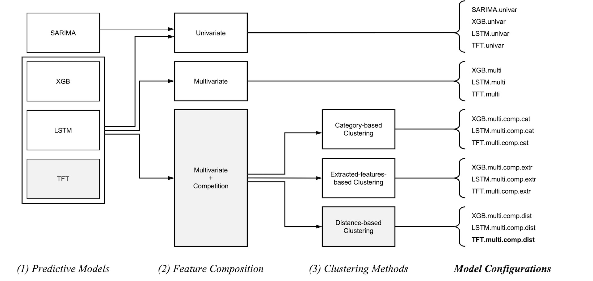
Figure 2: Study setup showing the resulting configurations of predictive models, feature compositions, and clustering methods in the scope of this paper. SARIMA is used as a benchmark model and only tested in a univariate configuration. The best-performing configuration is the Temporal Fusion Transformer based on multivariate features, including competitors’ data identified through distance-based clustering (highlighted in grey).

In our study, we test a variety of model configurations to identify the setup that performs best in predicting the future CPC of a sample of online advertisers. The core of each configuration is a predictive model. We selected four relevant model types representing different categories of time series forecasting approaches SARIMA as a statistical model, Extreme Gradient Boosting (XGB) from classical machine learning, Long short-term memory neural networks (LSTM) from deep learning, and the Temporal Fusion Transformer (TFT) representing novel transformer-based architectures.

Except for SARIMA, which is used as a univariate benchmark model, every model type is tested with three different compositions of input features: First, the model is only fed the univariate past cost-per-click data of the target advertiser. Second, in the multivariate setting, the set of features is extended to all data available for the target advertiser. Finally, we test if including data from a group of competing advertisers as further covariates improves predictive performance. Groups of competing advertisers are determined through time series clustering. As a benchmark, we use the advertisers’ primary category as cluster labels. We then adopt two proposed methods for time-series clustering: Extracted-features-based clustering and distance-based clustering.

Figure 2 shows how each of the 16 model configurations is put together. Every configuration is run iteratively to produce forecasts for every advertiser in scope. We evaluate the performance based on three forecasting horizons: 14 days, 30 days, and 60 days. Thereby we cover short-term forecasting, which in a practical application can be used for reacting to the current market situation, and long-term forecasting multiple months in advance for strategic budget planning. Finally, we compare models based on the aggregated average mean absolute error (MAE) and symmetric mean absolute percentage error (SMAPE) across all advertisers.

Predictive Models

Temporal Fusion Transformer

The Temporal Fusion Transformer (TFT) is an attention-based deep neural network architecture introduced by Lim et al. (2021) as a project within Google Cloud. In addition to producing accurate predictions across multiple forecasting horizons, this model stands out from other deep learning approaches by providing detailed interpretability of feature importances and temporal dynamics. With its inherent variable selection mechanism, the TFT is designed explicitly for multivariate big data problems. Successful applications in research involve predicting wind speed and traffic (Wu, Wang, and Zeng 2022; Zhang et al. 2022).

The TFT consists of multiple processing layers stacked on top of each other. In the first layer, all known, unknown, and static inputs are processed individually by variable selection networks (VSN). Features that do not contribute to model performance are filtered out. Furthermore, the selection is performed at each time step, which allows for the computation of feature importances for model interpretability.

Next is an LSTM encoder-decoder layer to perform locality enhancement. Hereby, the encoder LSTM is fed the known and unknown time series, while the decoder LSTM is only fed the known time series, both of which have previously been processed and weighted by the corresponding VSNs. The outputs of the locality enhancement layer are all provided to a gated residual network (GRN) committed to static enrichment. The GRN is an essential part of the TFT architecture and is also located under the hood of every individual VSN. It provides more freedom for the model to adjust the non-linear complexity for every input separately.

The final temporal self-attention layer captures long-term trends by accessing information from the far past. Compared to other transformer-based architectures, the TFT provides a multi-head attention mechanism, which enables interpretability. Each head learns distinct temporal patterns while attending to the same inputs. Overall attention can be computed across all heads and used for model interpretation (Fan et al. 2019).

Long Short-term Memory

Long Short-term Memory (LSTM) is an advanced deep learning architecture. Deep learning has generally been shown to be efficient in learning temporal patterns without the need for extensive preprocessing or feature engineering (Hochreiter and Schmidhuber 1997; Lim and Zohren 2021). In our data scope, the advertiser time series include multivariate features with a length of over a thousand daily observations. For forecasting problems of this complexity, deep learning models start to benefit from their ability to fit complex, non-linear functions and have proven to outperform statistical models reliably (Cerqueira, Torgo, and Soares 2019). In the LSTM architecture, each historical time step is represented in the network as an individual cell (Bahdanau, Cho, and Bengio 2014). As each cell corresponds to a historical time step, they can be fed the known and unknown time series. A multi-step output vector is computed from the final hidden state, fed through a linear layer to match the required length of the forecasting horizon. Through so-called gates, an LSTM learns the important parts of the input sequences while forgetting the less significant parts. They work best in application to long time series and are thus commonly used as a deep learning baseline for big data time series problems.

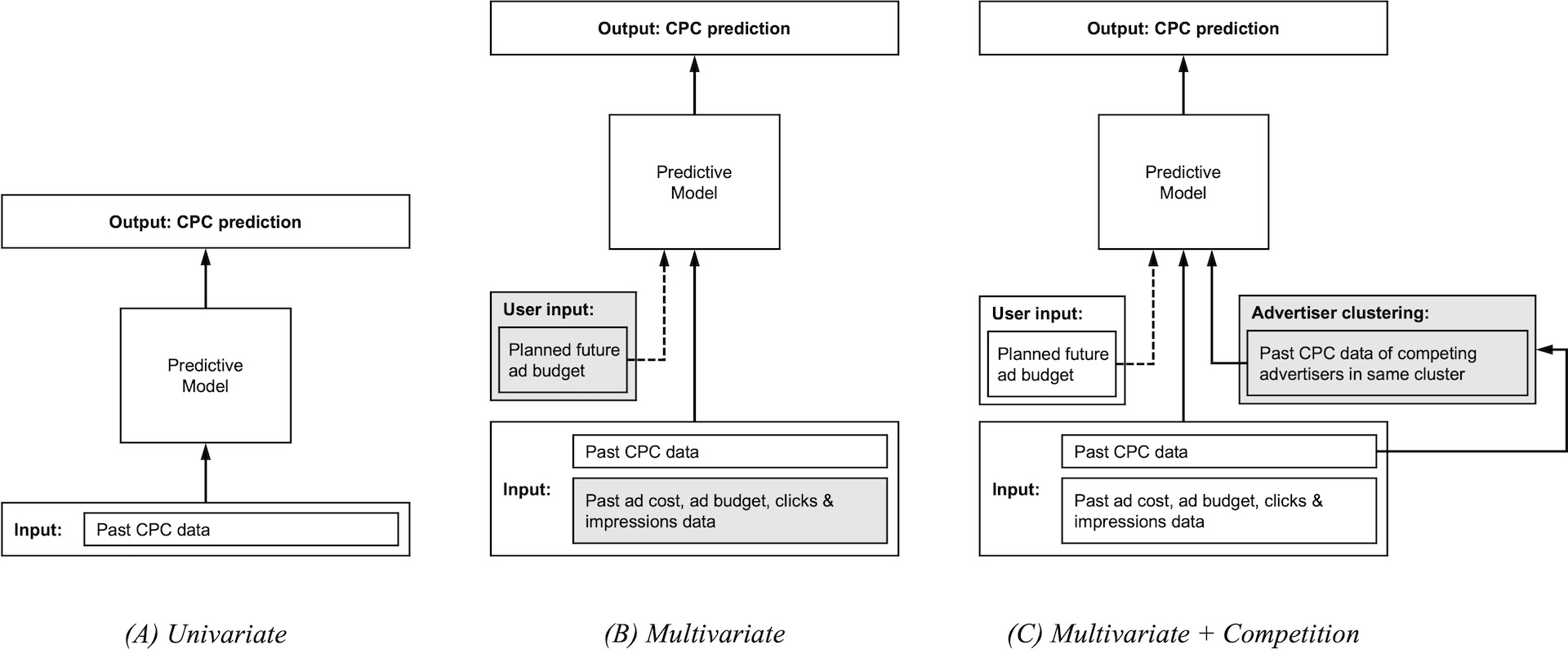
Figure 3: Feature composition set up for our three configurations (added component highlighted in grey).

Extreme Gradient Boosting

Extreme Gradient Boosting, or XGBoost, is an implementation of the Gradient Boosting Decision Trees (GBDT) ensemble learning algorithm. A trained model consists of several shallow decision trees, so-called weak learners, which are individually not meaningful. However, the weighted sum of all tree estimates together yields accurate final predictions. XGBoost was initially developed for classical machine learning disciplines such as classification, and regression (Chen and Guestrin 2016). However, by restructuring a time series dataset into a machine learning problem, the ensemble learning algorithm can also be applied to time series forecasting. Multi-step results are generated by fitting a separate model for each time step in the target sequence. Recent studies show that XGBoost time series forecasting achieves good scores in many domains and even outperforms complex deep learning models on some tasks (Elsayed et al. 2021). The predictions generated by an XGBoost model are inherently interpretable. The importance of each feature is calculated as its contribution to improving performance within each decision tree. The importance scores are then aggregated across all weak learners to obtain the overall interpretability of the predictions.

SARIMA

The Autoregressive Integrated Moving Average is a widely used statistical method for modeling univariate time series. In comparative studies, ARIMA models still outperform more complex approaches for univariate problems, especially on shorter time series, and is, therefore, as in our study, a common choice as a baseline model (Makridakis, Spiliotis, and Assimakopoulos 2018; Spiliotis et al. 2021). It consists of three components: The autoregressive component (AR) produces a forecast using a linear combination of the past values of the target variables’ own past values, while the moving average (MA) component models past forecasting errors. AR and MA themselves can only be applied to stationary series. Therefore, differencing of a certain degree is used as a third component to ensure stationarity. SARIMA extends the standard ARIMA method to support the direct modeling of a seasonal component. Three additional hyperparameters describing the nature of the seasonality to be captured, are required, as well as the number of time steps for a single seasonal period.

Feature Composition

The cost structures of online advertising are naturally driven by the competitive behavior of advertisers, which is intended and supported by Google through its keyword bidding architecture. Higher competition on certain keywords will inevitably lead to higher cost-per-click for the bidding parties. We aim to leverage these cost structures on an aggregated daily level to build multivariate forecasting models including the information of competing advertisers.

We experiment with feeding different compositions of features to our models. Thereby we can make assumptions about how much value lies in including additional information in relation to the increasing complexity of the problem and consequently, time to train the model. Figure 3 shows the three sets of features tested on each model. Every model is benchmarked against its simplest univariate configuration which solely learns from the historical CPC development (univariate). In the multivariate setup, we extend the data fed to the model by past information about ad cost, budget, clicks, and impressions of the individual target advertiser (multivariate). We furthermore include the planned ad budget, i.e. the model has access to the future budget level during the forecasting horizon since in a practical application this will be input by the user. In our final setup, we extract and include features describing the competitive landscape the target advertiser is part of. Competing advertisers are grouped using time-series clustering and the past CPC series of advertisers in the same cluster as the target are added as further covariates (multivariate + competition).

Clustering Methods

Category-based Clustering

The Google advertising data set provides information about the primary category to which each advertiser is assigned. We select this feature to use as labels for creating baseline clusters. Advertisers from the same industry are a natural choice for competing groups, as they are most likely to advertise similar products and services. Our category-based cluster assignment not only serves as a basis for performance comparison but also allows for subsequent analysis of the assignment of our two following data point-based methods. Insights will emerge about advertisers that are in direct competition across different categories, which can help to further improve predictive performance.

Extracted-features-based Clustering

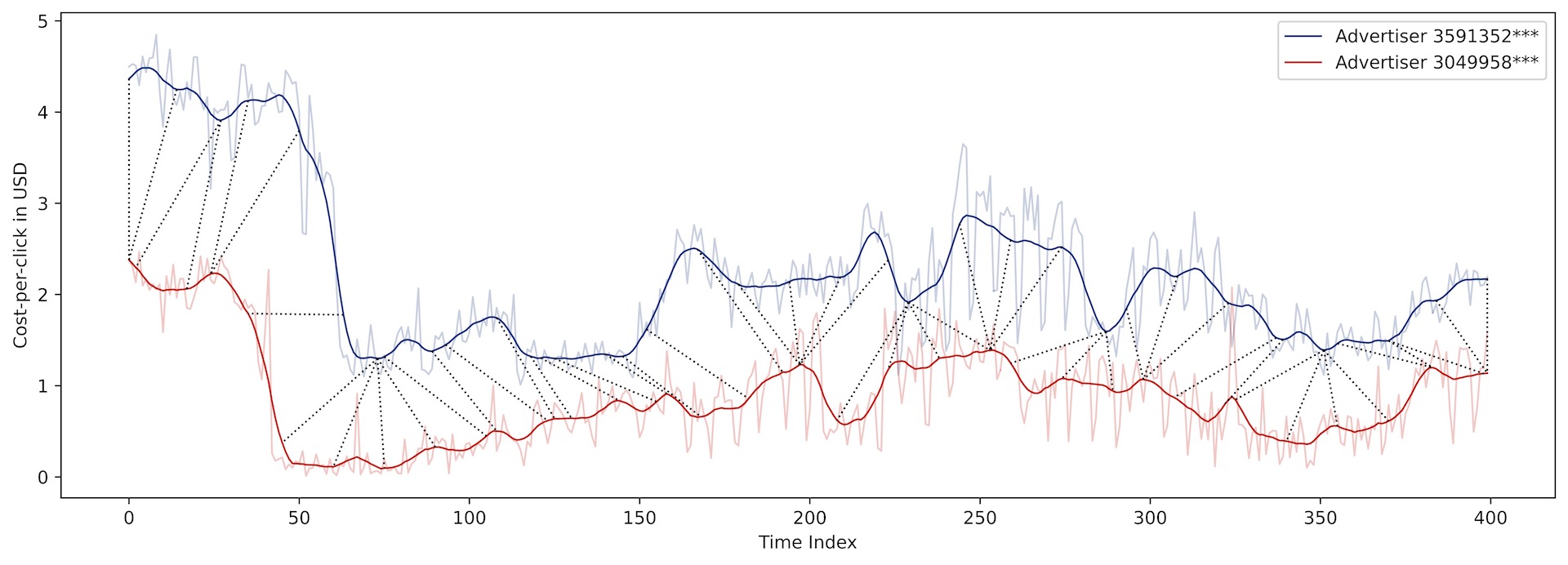
Figure 4: Example of matching two smoothed advertiser time-series using Dynamic Time Warping as a distance measure.

There are a variety of ways to extract features for time series clustering. The proposed methods range from generating a large number of features to represent the characteristics of the time series as accurately as possible, to extracting only selected descriptive features in order to avoid irritation from noise and outliers in the data. We follow the approach of Bandara, Bergmeir, and Smyl (2020), which states that a smaller number of high-level extracted features is more efficient for time series clustering. In addition, our third, distance-based method uses a large number of features, i.e., all raw data points, so using fewer but more informative features in this method allows for greater comparison. We generate 14 high-level descriptive features from each advertiser’s CPC time series, further described in Table 2. Based on the extracted numerical features, we apply the standard k-Means algorithm and choose the value of k according to the elbow method.

Extracted feature	Description
mean	Mean
variance	Variance
acf_1	First order of autocorrelation
trend	Strength of trend
linearity	Strength of linearity
curvature	Strength of curvature
season	Strength of seasonality
peak	Strength of peaks
trough	Strength of trough
entropy	Spectral entropy
lumpiness	Changing variance in remainder
spikiness	Strength of spikiness
f_spots	Flat spots using discretization
c_points	Number of crossing points

Table 2: Set of extracted time series features following Bandara, Bergmeir, and Smyl (2020)

Distance-based Clustering

We are using the time series k-Means algorithm (TSkmeans) introduced by Huang et al. (2016) to conduct our distance-based clustering of advertisers. TSkmeans solves existing problems of matching noisy time series by selecting smooth subspaces in the series and assigning weights to the time stamps that have the highest value for forming clusters. Furthermore, the TSkmeans algorithm leverages from averaging methods introduced by Petitjean, Ketterlin, and Gançarski (2011) to enable the usage of classical distance measures for matching serial data. The time-series k-means algorithm requires a distance measure to determine the similarity between two time-series. The most commonly used distance measures for time-series data are Euclidean distance and Dynamic Time Warping (DTW).

Euclidean distance is a simple and intuitive measure of similarity, it calculates the straight-line distance between two points in a multidimensional space. However, it is not suitable for time-series data because it assumes that the time-series are aligned and have the same length. This assumption is often violated in practice, making Euclidean distance a poor choice for time-series data. For example, if two time-series have similar patterns but one is shorter or longer than the other, the Euclidean distance will be large even though the patterns are similar.

Dynamic Time Warping (DTW) was introduced to solve the weaknesses of the Euclidean distance metric in application to time series (Berndt and Clifford 1994). DTW is a distance measure that addresses the alignment problem by warping the time-series in a non-linear fashion. It allows for differences in time scales and non-uniform sampling rates, making it a more robust distance measure for time-series data. DTW is defined as the minimum accumulated distance between two time-series, where the distance between two points is calculated as the Euclidean distance and the accumulated distance is computed by moving through a matrix of pairwise distances, with the restriction of not being able to move diagonally to the left. This restriction ensures that the time-series are aligned before computing the distance, making it more robust to variations in time scales and non-uniform sampling rates. Figure 4 demonstrates, how DTW allows for the alignment of two smoothed advertiser time series, where similar patterns are shifted in time and occur in different scales.

DTW has been proven to be a more accurate and robust distance measure for time-series data than Euclidean distance (Ratanamahatana and Keogh 2005). In speech recognition, DTW has been shown to improve recognition rates over Euclidean distance because it is able to align different spoken versions of the same word (Amin and Mahmood 2008). In bioinformatics, DTW has been used to align protein sequences and has been shown to be more effective than Euclidean distance in identifying similar patterns (Aach and Church 2001).

Model		14 days			30 days			60 days
		MAE $\downarrow$	SMAPE $\downarrow$		MAE $\downarrow$	SMAPE $\downarrow$		MAE $\downarrow$	SMAPE $\downarrow$
SARIMA.univar		0.211	0.179		0.227	0.197		0.306	0.264
XGB.univar		0.259	0.225		0.278	0.243		0.340	0.279
XGB.multivar		0.242	0.218		0.271	0.231		0.274	0.258
XGB.multivar.comp.cat		0.245	0.219		0.250	0.218		0.278	0.423
XGB.multivar.comp.extr		0.248	0.228		0.257	0.216		0.267	0.239
XGB.multivar.comp.dist		0.244	0.213		0.246	0.227		0.276	0.235
LSTM.univar		0.245	0.203		0.265	0.217		0.318	0.251
LSTM.multivar		0.235	0.204		0.250	0.215		0.252	0.236
LSTM.multivar.comp.cat		0.231	0.199		0.229	0.202		0.253	0.228
LSTM.multivar.comp.extr		0.227	0.202		0.235	0.199		0.253	0.237
LSTM.multivar.comp.dist		0.229	0.196		0.231	0.210		0.250	0.232
TFT.univar		0.216	0.185		0.236	0.204		0.307	0.241
TFT.multivar		0.203	0.180		0.223	0.192		0.241	0.214
TFT.multivar.comp.cat		0.208	0.181		0.215	0.188		0.238	0.204
TFT.multivar.comp.extr		0.207	0.181		0.211	0.186		0.235	0.202
TFT.multivar.comp.dist		0.201	0.177		0.216	0.183		0.232	0.196

Table 3: Model performance comparison of all model and clustering configurations in three forecasting horizons

Results

Model Performance Comparison

The final scores for every model configuration and each of the three forecasting horizons are demonstrated in Table 3. The overall best-performing model in our evaluation setup is the Temporal Fusion Transformer, including competing advertiser timer series identified through distance-based clustering as covariates. Especially in the longest forecasting horizon tested (60 days), this configuration outperforms all other models across all three performance measures. Notably, univariate SARIMA performs well on shorter forecasting horizons. For longer horizons however, the performance drops rapidly and SARIMA is outperformed by more complex models including multivariate features.

We observe, that for all tested models the best configuration is always based on clustered multivariate features from competitors included as covariates. Except for the 14-day XGBoost and the 14-day LSTM prediction, where the best performance was obtained by category-based and extracted-features-based clustering respectively, the best performance is consistently achieved through distance-based clustering in terms of SMAPE. Our results thus stand in contrast to Bandara, Bergmeir, and Smyl (2020), who apply clustering based on extracted features on the assumption that few high-level descriptive features serve better as a basis for selecting groups of relevant time series to use as covariates. We find, that clustering based on the actual data points of the time series using Dynamic Time Warping selects better clusters in terms of achieving superior SMAPE scores. Interestingly, using the advertiser categories as clusters was outperformed by both of the clustering algorithms in almost every test scenario. We can think of two possible explanations for this result: First, we have 21 advertiser categories in our data set as opposed to six and seven clusters created by the clustering algorithms. Especially XGBoost and the TFT inherently perform different processes to filter relevant features. Consequently, feeding them a larger group of exogenous advertiser time series bears a higher likelihood of filtering relevant ones that contribute to improving model performance. Second, online advertisers may be in competition with parties from other categories. The better-performing algorithm-generated clusters represent the advertiser categories only to a certain degree, as further analyzed in section 4.2, which may indicate that there are cross-categorical competitive patterns that help to improve predictions.

The tested models can be grouped into three categories: Statistical models, machine learning, and deep learning. We find that, for the advertisers and time frame in scope, deep learning models, namely LSTM and TFT, perform best overall. SARIMA as a statistical model performs well in shorter horizons, but for long-term forecasting, the statistical approach decreases strongly in performance. XGBoost, LSTM, and TFT as machine and deep learning models especially in the multivariate configurations show a more stable development of the forecasting errors with increasing horizon length.

We also find, that for all models the univariate configuration decreases stronger in performance over longer horizons than the multivariate. This could be due to the budget data, which multivariate models include as a covariate. As further explained in the section on Model Explainability, the CPC development is highly dependent on the advertisers’ budget input which occurs on the monthly level. Therefore, models that have access to the budget information and are complex enough to learn the monthly input structure, in our tests mainly the deep learning models, perform better in predicting the monthly level changes for forecasting horizons longer than a month. Our results support this since for all models the univariate prediction performance decreases strongly, similar to the univariate statistical models, while the multivariate prediction performances remain more stable.

Lastly, we find that our identified best model, the TFT, has the smallest performance difference between the three clustering configurations. Transformers have proven to work best with large amounts of data i.e. long time series and a large number of features. Especially the Temporal Fusion Transformer architecture used in our research includes an inherent layer of variable selection networks dedicated to filtering the most relevant variables. The model is therefore likely to assign the highest weights to a group of a few highly relevant exogenous advertiser time series that are included in the same cluster according to all three clustering approaches.

Cluster Assignment

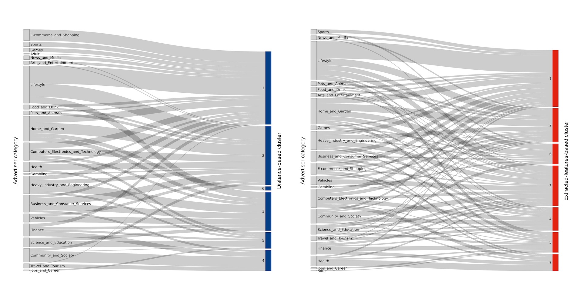
Figure 5: Sankey diagram of cluster assignments using the distance-based (left) and extracted-features-based approach (right) compared to the advertisers’ native category.

Our two clustering assignments, generated by applying k-Means to a distance-based representation and an extracted-feature-based representation of advertisers’ cost-per-click time series, differ from each other and also from the advertiser categories we use as baseline clusters.

Following the elbow method, the distance-based approach assigns advertisers to six clusters. We observe a strong representation of the advertiser categories in the assignment, as larger groups of advertisers stemming from the same category tend to be also located in the same clusters. More than half of the advertisers are assigned to two large clusters, while more interestingly, the four smaller clusters include a selected combination of advertisers from different categories. The Sankey visualization technique applied in Figure 5 sorts the source and target nodes to optimize towards a clean layout. We can not only track the exact category composition of each cluster but also make assumptions about categories that might be correlated in their CPC development through algorithmic sorting of the nodes: Advertiser categories that are close to each other in the visualization share a similar pattern of cluster assignment. For distance-based clustering, this means that interestingly the connected advertisers show a similar development of their CPC, although they often come from different categories. Examples of connected categories that make sense in context are ”Sports” and ”Games” or ”E-commerce & Shopping” and ”Lifestyle” which are mainly located in cluster 1.

For k-Means clustering based on the extracted features, the elbow method suggests seven clusters. In contrast to distance-based clustering, we do not find a strong representation of advertiser categories in the clusters. It is already visually apparent that the resulting clusters consist of mixtures of much smaller advertiser subgroups. The advertisers for most categories are well distributed across multiple clusters. One possible explanation is that the high-level descriptive features do not reflect the local patterns of the time series well enough to cluster the advertisers of the same category. Instead, clustering is based on more general characteristics such as mean CPC value and distribution. Spontaneous spikes or level changes that would be captured by distance-based clustering are unlikely to be accounted for in the assignment of extracted-feature-based clustering and may be an explanation for the identified poorer multivariate prediction results as these rely heavily on local similarities between the target and the exogenous time series.

Model Explainability

Feature importance of the Temporal Fusion Transformer is analyzed by interpreting its Variable Selection Networks (VSNs), which produce sparse weights for static, encoder, and decoder inputs. Furthermore, all attention heads of the TFT share the same weights, so the overall attention can be computed by aggregation across the individual heads.

Figure 6 demonstrates, how the TFT predicts a 60-day CPC forecast for two exemplary advertisers. We include temporal attention as a heatmap behind the time stamps and the encoder and decoder feature importance in sorted bar charts in the visualization. We further plot the average CPC of the advertisers within the same cluster. We intentionally selected two advertisers with different structural patterns to demonstrate the adaptability of our TFT process for individual groups of time series.

In the first example, we predict an advertiser with a strong underlying weekly seasonality in his CPC. As we can further observe, in the past CPC data plotted, the weekly seasonality that is predicted by the model is visually actually not as present, at least in the represented time window. The encoder’s importance tells us, that one competing advertiser is highly important for model training. The advertiser’s inherent features CPC and 7-day lagged CPC are comparatively unimportant. Consequently, the model is likely to learn the level and seasonality not only within the advertisers’ own data but primarily in the data of one or multiple competing advertisers. The prediction does not only accurately represent the short-term fluctuations of the future CPC, but also follows the increasing peaks and amplitude in the long term.

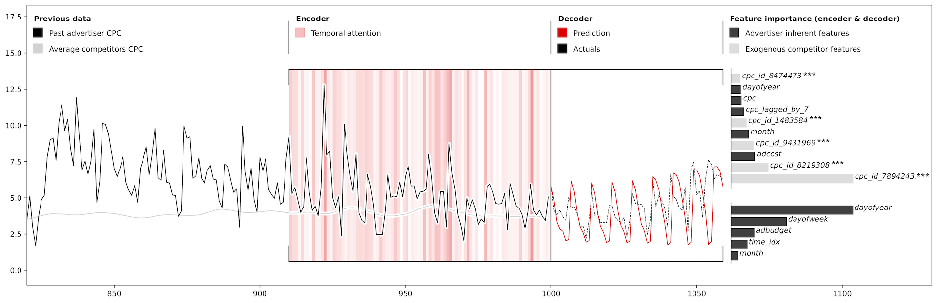
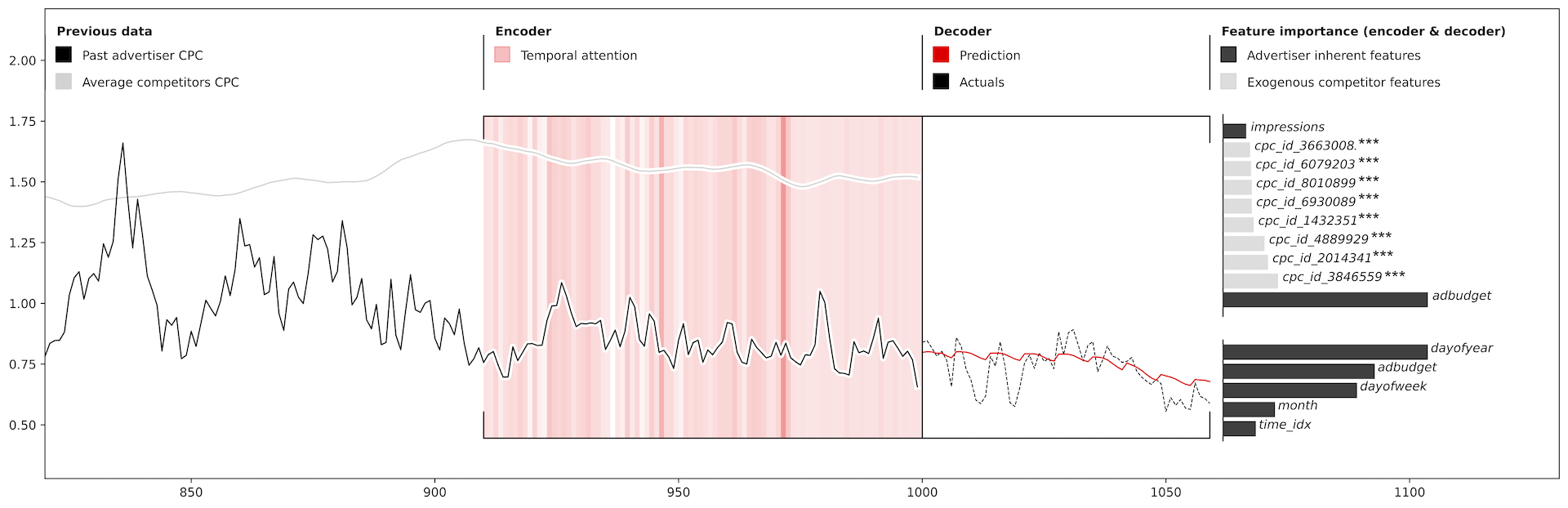
Figure 6: Exemplary 60-day predictions of our proposed model for two selected advertisers showing different underlying CPC structures. We highlight the temporal attention to the encoder time steps in red, indicate the encoder (top) and decoder (bottom) feature importance as bar charts, and plot the average CPC of the advertisers in the same clusters as a grey line.

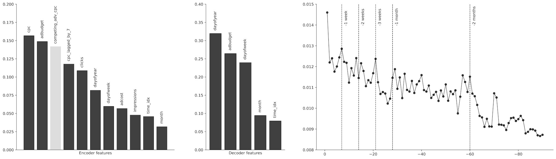
Figure 7: Average feature importance and temporal attention across all advertiser models. The weights dedicated to competing advertiser’s CPC features are summed up to one bar in the encoder highlighted in grey.

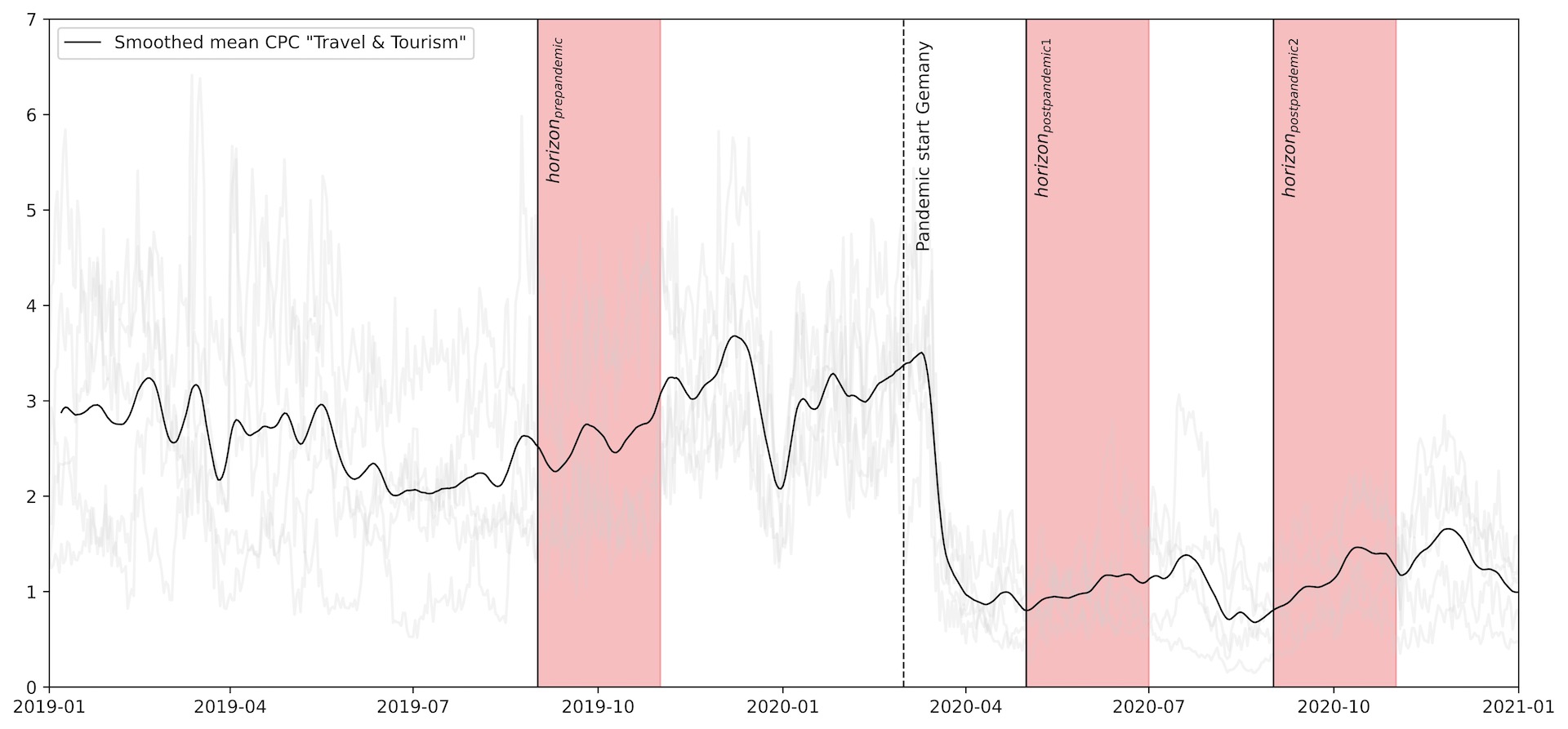
Figure 8: Pandemic impact on the average CPC of six advertisers from “Travel & Tourism” with highlighted forecasting horizons to test model performance in different stages of the crisis

Horizon	TFT.multivar	TFT.multivar.comp.dist
Pre-Pandemic (2019-09 and 2019-10)	$0.244\pm 0.193$	$0.227\pm 0.124$
Post-Pandemic 1 (2020-05 and 2020-06)	$0.750\pm 0.544$	$0.687\pm 0.413$
Post-Pandemic 2 (2020-09 and 2020-10)	$0.528\pm 0.339$	$0.329\pm 0.162$

Table 4: Performance improvement measured by mean SMAPE across six advertisers from “Travel & Tourism” over three forecasting horizons by including clustered competitors’ data as covariates

The second example advertiser does not show a strong weekly seasonality. Looking at the encoder and decoder importances, the monthly advertising budget seems to be a central factor for the development of this advertiser’s CPC. The TFT prediction captures a strong decrease in the future CPC which is most likely influenced by a change in the planned future advertising budget. The model manages to accurately convert this input information into a smooth decrease of the CPC level in the long term, reflecting what it has learned from the past CPC reactions to ad budget adaptions.

Figure 7 further shows the average feature importance and temporal attention across all advertiser models that we have trained. All encoder importance dedicated to competing advertisers’ CPCs is summed up in one bar. Unsurprisingly, the past values of the target variable, CPC, are most important for the encoder. Additionally, the advertising budget and the competing advertisers dominate the variable selection of the encoder, followed by the day of the week supporting the modeling of weekly seasonalities, which is often present in the series.

The decoder outputs the importance of the features for which the future values are known. Most weight is assigned to the day of the year, which is likely due to special days like Christmas, where a lot of competition is present in the online advertising market and consequently CPCs tend to spike up on the same days every year. Important is also the advertising budget and day of the week to determine the accurate level and seasonality of the prediction.

Lastly, Figure 7 includes the average temporal attention to the time steps in the encoder. Apart from the last available time step, which is assigned the largest importance, the weights decrease rather constantly going back in time. We observe weight peaks around time steps that naturally represent seasonality cycles, i.e. every seven days over the first month and also in the long run roughly every new month.

Policy Experiment

A prevalent problem in deep learning of long time-series data are large distortions in the training data associated with one-time external events, e.g., economic crises. Significant changes in the data can prevent Deep Learning models from detecting consistent patterns, resulting in lower predictive performance. The time frame chosen for our study spans the beginning of the Covid 19 pandemic. In our geographical data scope, Germany, the first restrictions on public life, including contact restrictions and cancellations of major events, began in March 2020. One sector that was severely affected by this crisis is travel and tourism. As uncertainty about further restrictions increased, customers postponed booking their summer vacations or canceled existing plans.

We are interested in the robustness of our proposed model that leverages information about related advertisers within or outside their industry. Therefore, we select all advertisers from the “Travel & Tourism” category in our data scope and test the performance of two models, one that incorporates competing advertisers (TFT.multivar.comp.dist), which was the best-performing model in our previous tests, and a simpler version of this model that only considers each advertiser’s own characteristics, such as past cpc, clicks, and budget (TFT.multivar). We further select three forecasting horizons for comparison: First, a time window prior to the onset of the pandemic in Germany (September and October 2019) to test the performance of the models trained on one and a half years of relatively stable data without significant level changes. Second, a window immediately after the onset of the pandemic (May and June 2020), where the direct impact of public and travel restrictions on the online advertising market is represented not only in the training data but also in the 90-day encoder window of the specific forecast. And finally, a window a few months after the pandemic outbreak (September and October 2020) to compare how well the two models adapt to the new situation in terms of predictive performance.

Figure 8 shows the three forecast horizons and the average CPC development of the selected advertisers from “Travel & Tourism”. Interestingly, we observed a sudden drop in the CPC level immediately after the start of the pandemic, meaning that advertising got significantly cheaper. In the following, the CPCs remain low for the duration of the first pandemic year in Germany. A further investigation of the variables shows that advertisers reacted immediately after the pandemic outbreak by substantially reducing their advertising budget. The lowered costs for advertising could represent Google’s reaction. Shortly after, advertisers increased their budgets again in the summer of 2020 to almost the same level as before. However, conversion to clicks remained high, resulting in consistently lower cost-per-click over the course of the first pandemic year.

Table 4 shows the results of our robustness experiment. In the first forecasting horizon, we observe a difference in performance between the models that is consistent with our overall results (previously shown in Table 3): The TFT trained with competing advertisers (TFT.multivar.comp.dist) achieves a slightly better SMAPE but predictions are at a similar level to those of the multivariate TFT that is only fed the advertisers’ inherent features (TFT.multivar). In the second horizon, both models achieve drastically worse performance. The CPC level change in the encoder window distorts the predictions, although the TFT.multivar.comp.dist still achieves a better score. The last horizon shows that our proposed model learns more reliably and performs better when trained on long data series that include drastic changes in past target variable development. Including competing advertisers as features for the model, training helps to learn better the connected patterns of budget, ad cost, clicks, and resulting CPC and is less affected by large changes in the training data.

Conclusion

Summary

This study aims to forecast online advertising cost-per-click for advertisers in different industries over multiple time horizons using a large-scale paid search dataset. Several time-series forecasting techniques were applied, including statistical methods, machine learning models, and deep learning models. We further experiment with adding additional features from the advertiser itself, as well as from similar advertisers to set up multivariate baseline configurations. Three time-series clustering approaches were adopted to identify relevant covariates within the expansive advertiser landscape.

Our results show that the Temporal Fusion Transformer architecture using CPC from related advertisers within the same cluster identified through distance-based clustering obtains the best performance across all model and clustering configurations in three forecasting horizons. Furthermore, we analyzed the feature importance and temporal attention output to interpret the model predictions and demonstrated how the model learns weekly and monthly seasonality, as well as CPC information from related advertisers within the same cluster, and captured the non-linear effect of budget levels on the CPC.

Lastly, we show that our approach may provide robust predictions when the online advertising market experiences significant changes, e.g., COVID-19 pandemic. Compared to model configurations with the same architecture with only the focal advertiser’sCPC information, i.e., a model that individual advertisers would be able to build themselves, our approach shows consistently better performance across different time horizons.

We contribute to existing approaches in the online advertising community by proposing a scalable technique to select relevant covariates from a wide pool of advertisers that contribute to improving multi-horizon prediction performance. Our approach also enables individual advertisers to input future budget plans and receive accurate long-term forecasts using patterns observed in the past. The separate elements of our proposed forecasting pipeline can further be used for other tasks: Many advertisers in the dataset are not natively assigned to a category. Using the distance-based clustering method from our study, advertisers organically form groups which help to determine a category. Our technique is furthermore not only helpful for forecasting but can be used to accurately close existing gaps for advertisers’ time series in the database, especially when signals of the majority of advertisers within the cluster are existent.

Business Context

Google has started changing their presentation of keyword level information in their ad tool ”keyword planner”. Where as before you were only provided a mean CPC for a given keyword, you are now given two values of ”low range” and ”high range” price values. This makes your keyword level assignments of your max cpc bidding strategies easier since you are now able to estimate if your are in the upper or lower max CPC area - but the values are static on monthly levels and do not take into account future events like black Friday, Christmas seasons or similar predictable events. This research paper has shown the far more accuracy in predicting campaign or website level CPCs are possible and will be invaluable for assessing budget viability for a long future horizon. In the highly competitive adspace both small to medium and large online businesses will gain an edge over the competition by being able to shift budgets over longer periods of time maximize ad effectiveness within their seperate monetary constraints. For the former, it will be possible to ”choose your battles wisely” and shift budgets into times of less competitive CPCs in order to maximize the ROAS in the respective phases. In contrast, the latter companies with a larger budget should fully allocate budgets into the high demand CPC phases. Many more strategies are of course possible which are all enabled by a more accurate prediciton of future CPC behaviour.

Outlook

The strong correlations of CPC changes between industries of all facets give rise to both more in-depth research and an obligation for practitioners to broaden their horizons. They should not only look at the CPCs developments and corresponding predictions within their own sector. They will also need to go further than looking at the overall adspends in their entirety. To truly get the best predictions, our models have shown that it is essential to examine non-obvious connections between advertisers, often from different industries, as identified in our study through distance-based clustering. Further research on the actual keyword level is necessary to explore the advertising connections across the industries.

From an overall Analytics perspective, there are of course even more metrics of interest that would benefit from the proposed techniques in this paper. Predicting your overall revenue, number of transaction, the cost-per-acquistion or ROAS would be a significant help for multiple decision makers of online marketing teams. All of the metrics are inherently intertwined with market and competitor behaviours so it is likely that the same techniques will yield promising results.

Recent advances in the development of Graph Neural Networks (GNN), which use either static or temporal dynamic graph representations of a network of series, seem to be well suited for modeling the competitive landscape of online advertising (Wu et al. 2020; Cui et al. 2021). It would be interesting to compare the performance obtained first by the proposed graph generation based on the distances of the multivariate series, as in this study but on a smaller granularity, and second by a manual graph structure based on the keyword data available in our database, where each node is an advertiser and the weight of the edges is the number of shared keywords.

References

- Aach and Church (2001) Aach, J.; and Church, G. M. 2001. Aligning gene expression time series with time warping algorithms. Bioinformatics, 17(6): 495–508.
- Amin and Mahmood (2008) Amin, T. B.; and Mahmood, I. 2008. Speech recognition using dynamic time warping. In 2008 2nd international conference on advances in space technologies, 74–79. IEEE.
- Bahdanau, Cho, and Bengio (2014) Bahdanau, D.; Cho, K.; and Bengio, Y. 2014. Neural Machine Translation by Jointly Learning to Align and Translate.
- Bandara, Bergmeir, and Smyl (2020) Bandara, K.; Bergmeir, C.; and Smyl, S. 2020. Forecasting across time series databases using recurrent neural networks on groups of similar series: A clustering approach. Expert Systems with Applications, 140(112896).
- Berndt and Clifford (1994) Berndt, D. J.; and Clifford, J. 1994. Using Dynamic Time Warping to Find Patterns in Time Series. In KDD ’94, 10th ACM SIGKDD International Conference on Knowledge Discovery & Data Mining, 359–370.
- Cerqueira, Torgo, and Soares (2019) Cerqueira, V.; Torgo, L.; and Soares, C. 2019. Machine Learning vs Statistical Methods for Time Series Forecasting: Size Matters.
- Chen and Guestrin (2016) Chen, T.; and Guestrin, C. 2016. XGBoost: A Scalable Tree Boosting System. In Proceedings of the 22nd ACM SIGKDD International Conference on Knowledge Discovery and Data Mining, KDD ’16, 785–794. New York, NY, USA: Association for Computing Machinery. ISBN 9781450342322.
- Cui et al. (2021) Cui, Y.; Zheng, K.; Cui, D.; Xie, J.; Deng, L.; Huang, F.; and Zhou, X. 2021. METRO: a generic graph neural network framework for multivariate time series forecasting. Proceedings of the VLDB Endowment, 15(2): 224–236.
- Dentsu (2022) Dentsu. 2022. Global Ad Spend Forecast July 2022.
- Elsayed et al. (2021) Elsayed, S.; Thyssens, D.; Rashed, A.; Jomaa, H. S.; and Schmidt-Thieme, L. 2021. Do We Really Need Deep Learning Models for Time Series Forecasting?
- Fan et al. (2019) Fan, C.; Zhang, Y.; Pan, Y.; Li, X.; Zhang, C.; Yuan, R.; Wu, D.; Wang, W.; Pei, J.; and Huang, H. 2019. Multi-horizon time series forecasting with temporal attention learning. In Proceedings of the 25th ACM SIGKDD International conference on knowledge discovery & data mining, 2527–2535.
- Google (2022) Google. 2022. How AdSense works.
- Hochreiter and Schmidhuber (1997) Hochreiter, S.; and Schmidhuber, J. 1997. Long short-term memory. Neural computation, 9(8): 1735–1780.
- Huang et al. (2016) Huang, X.; Ye, Y.; Xiong, L.; Lau, R. Y.; Jiang, N.; and Wang, S. 2016. Time series k-means: A new k-means type smooth subspace clustering for time series data. Information Sciences, 367-368: 1–13.
- Irvine (2022) Irvine, M. 2022. Google Ads Benchmarks for YOUR Industry [Updated!].
- Lim et al. (2021) Lim, B.; Arık, S.; Loeff, N.; and Pfister, T. 2021. Temporal Fusion Transformers for interpretable multi-horizon time series forecasting. International Journal of Forecasting, 37(4): 1748–1764.
- Lim and Zohren (2021) Lim, B.; and Zohren, S. 2021. Time-series forecasting with deep learning: a survey. Philosophical Transactions of the Royal Society A: Mathematical, Physical and Engineering Sciences, 379(2194): 20200209.
- Makridakis, Spiliotis, and Assimakopoulos (2018) Makridakis, S.; Spiliotis, E.; and Assimakopoulos, V. 2018. Statistical and Machine Learning forecasting methods: Concerns and ways forward. PLoS ONE, 13(3): e0194889.
- Petitjean, Ketterlin, and Gançarski (2011) Petitjean, F.; Ketterlin, A.; and Gançarski, P. 2011. A global averaging method for dynamic time warping, with applications to clustering. Pattern Recognition, 44(3): 678–693.
- Ratanamahatana and Keogh (2005) Ratanamahatana, C. A.; and Keogh, E. 2005. Three myths about dynamic time warping data mining. In Proceedings of the 2005 SIAM international conference on data mining, 506–510. SIAM.
- Spiliotis et al. (2021) Spiliotis, E.; Makridakis, S.; Semenoglou, A.-A.; and Assimakopoulos, V. 2021. Comparison of statistical and machine learning methods for daily SKU demand forecasting. Operational Research, 22: 3037–3061.
- Wu, Wang, and Zeng (2022) Wu, B.; Wang, L.; and Zeng, Y.-R. 2022. Interpretable wind speed prediction with multivariate time series and temporal fusion transformers. Energy, 252: 123990.
- Wu et al. (2020) Wu, Z.; Pan, S.; Long, G.; Jiang, J.; Chang, X.; and Zhang, C. 2020. Connecting the dots: Multivariate time series forecasting with graph neural networks. In Proceedings of the 26th ACM SIGKDD international conference on knowledge discovery & data mining, 753–763.
- Yang et al. (2022) Yang, Y.; Zhao, K.; Zeng, D. D.; and Jansen, B. J. 2022. Time-varying effects of search engine advertising on sales–An empirical investigation in E-commerce. Decision Support Systems, 163: 113843.
- Yuan, Wang, and Zhao (2013) Yuan, S.; Wang, J.; and Zhao, X. 2013. Real-time Bidding for Online Advertising: Measurement and Analysis. In Seventh International Workshop on Data Mining for Online Advertising, 1–8.
- Zenith (2022) Zenith. 2022. Advertising Expenditure Forecasts December 2021.
- Zhang et al. (2022) Zhang, H.; Zou, Y.; Yang, X.; and Yang, H. 2022. A temporal fusion transformer for short-term freeway traffic speed multistep prediction. Neurocomputing, 500: 329–340.