Individualized Treatment Allocation in Sequential Network Games

Abstract

Designing individualized allocation of treatments so as to maximize the equilibrium welfare of interacting agents has many policy-relevant applications. Focusing on sequential decision games of interacting agents, this paper develops a method to obtain optimal treatment assignment rules that maximize a social welfare criterion by evaluating stationary distributions of outcomes. Stationary distributions in sequential decision games are given by Gibbs distributions, which are difficult to optimize with respect to a treatment allocation due to analytical and computational complexity. We apply a variational approximation to the stationary distribution and optimize the approximated equilibrium welfare with respect to treatment allocation using a greedy optimization algorithm. We characterize the performance of the variational approximation, deriving a performance guarantee for the greedy optimization algorithm via a welfare regret bound. We establish the convergence rate of this bound. We implement our proposed method in simulation exercises and an empirical application using the Indian microfinance data (Banerjee et al., 2013), and show it delivers significant welfare gains.

Keywords: Treatment choice, Markov random field, Gibbs distribution, variational approximation, mean field games, graphical potential game.

1 Introduction

The question of how best to allocate treatment to units interacting in a network is relevant to many policy areas, including the provision of local public goods (Bramoullé and Kranton, 2007), the diffusion of microfinance (Banerjee et al. (2013); and Akbarpour et al. (2020)), and strategic immunization (Galeotti and Rogers (2013); and Kitagawa and Wang (2023)). Obtaining an optimal individualized allocation, however, is often infeasible due to analytical and computational challenges. As a consequence, practical counterfactual policy analysis in the presence of network spillovers is limited to simulating and comparing outcome distributions or welfare values across a few benchmark candidate policies. This leaves the magnitude of the potential welfare gains of an optimal individualized assignment policy unknown.

Focusing on a class of social network models in which interacting agents play sequential decision games (Mele (2017); and Christakis et al. (2020)), this paper develops a method to obtain optimal treatment assignment rules that maximize a social welfare criterion. We consider an individualized allocation of binary treatments over agents who are heterogeneous in terms of their own observable characteristics, their network configurations, and their neighbors’ observable characteristics. Each agent chooses a binary outcome so as to maximize their own utility. This choice depends upon the agent’s own characteristics and treatment as well as their neighbors’ characteristics, treatments and choices. The sequential decisions of randomly ordered agents induce a unique stationary distribution of choices (Mele, 2017). We specify the planner’s welfare criterion to be the mean of the aggregate outcomes (i.e., the sum of the means of binary outcomes over all agents in the network) at the stationary state that is associated with a given treatment allocation. We aim to maximize the welfare evaluated at the stationary outcome distribution with respect to the individualized allocation of treatments.

There are analytical and computational challenges to solving the maximization problem for optimal targeting. First, fixing an allocation of treatments, the sequential decision games induce a Markov random field (MRF) and the stationary outcome distribution has a Gibbs distribution representation. The analytical properties of the mean of the aggregate outcomes, however, are difficult to characterize. To approximate the joint distribution of outcomes, the literature on MRFs performs numerical methods such as Markov Chain Monte Carlo (MCMC) (Geman and Geman, 1984). If the size of the network is moderate to large though, MCMC can be slow to converge. It is, therefore, infeasible to perform MCMC to evaluate the welfare at every candidate treatment assignment policy. Second, obtaining an optimal individualized assignment is a combinatorial optimization problem with respect to a binary vector whose cardinality is equal to the number of agents in the network. A brute force search quickly becomes infeasible as the size of network expands.

We tackle these challenges by proposing methods for approximately solving the combinatorial optimization problem for individualized assignment. Our proposal is to perform a variational approximation of the stationary distribution of outcomes and to optimize the approximated equilibrium welfare with respect to an assignment vector by using a greedy optimization algorithm. The variational approximation step lessens the computational burden of running MCMC at each candidate policy. The greedy optimization step reduces the computational burden of the combinatorial optimization by assigning treatment sequentially to the agent who generates the largest welfare gain given previous assignments. Since our proposal involves approximation of the objective function and the heuristic method of greedy optimization, our proposal is not guaranteed to lead to a global optimum. A novel contribution of this paper is that we derive a performance guarantee for our proposed method in terms of an analytical upper bound on the welfare loss relative to the globally optimal assignment. The upper bound on the welfare regret consists of two terms: the welfare loss due to variational approximation and the welfare loss due to greedy optimization. We show that, once scaled such that it can be interpreted as the per-person welfare loss, the first term of the upper bound on the welfare loss (originating from the variational approximation) vanishes asymptotically as the number of agents in the network increases. On the other hand, we show that the second term of the upper bound on the the welfare loss (originating from the greedy optimization) does not generally converge to zero.

To highlight this paper’s unique contributions to the literature, we abstract from estimation of the structural parameters underlying the sequential decision game and assume that they are known. See Geyer and Thompson (1992), Snijders et al. (2002), Wainwright et al. (2008), Chatterjee and Diaconis (2013), Mele (2017), Boucher and Mourifié (2017), and Mele and Zhu (2022) for identification and estimation of these parameters. In practical terms, our proposed method is useful for computing an optimal assignment of treatment, with point estimates plugged-in in place of structural parameters.

To assess the performance of our proposal, we perform extensive numerical studies. Given that the number of possible configurations increases exponentially with the size of the network, we are only able to apply the brute force method to search for the optimal allocation rule in a small network setting. We find that our proposed method leads to a globally optimal solution in a small network setting under our assumptions. In a large network setting, we first examine the performance of using our method compared with No treatment and with random allocation. We attain a welfare improvement of around $50\%$ relative to a No treatment rule, and an improvement of around $10\%$ relative to a random allocation rule. In addition, we evaluate the welfare performance gap of using variational approximation compared with MCMC to approximate the stationary distribution of the outcome. Under our assumptions, the variational approximation performs as well as MCMC for all of the treatment allocation rules that we consider.

We augment these numerical studies with an empirical application that illustrates the implementation and welfare performance of our method. Specifically, we apply our procedure to Indian microfinance data that has been previously analyzed by Banerjee et al. (2013). The data contains information about households in a number of villages, their relation to other households in their village, and whether they chose to purchase a microfinance product. For each village in the sample, we estimate the structural parameters of an assumed utility function using the method outlined in Snijders et al. (2002). Plugging in the parameter estimates, we obtain an individualized treatment allocation rule using our greedy algorithm. We compare the village welfare attained by our greedy algorithm with the welfare achieved by an NGO called Bharatha Swamukti Samsthe (BSS). For all $43$ villages in the sample, our method is associated with a higher welfare-level, with the magnitude of improvement varying from $9.82\%$ to $137.46\%$ (average improvement is $40.69\%$). The magnitude of the welfare gain is remarkable and demonstrates the benefits of individualized targeting under interference.

The remainder of this paper is organized as follows. We first review the relevant literature in the remainder of this section. Section 2 details the sequential decision process and the stationary distribution of the outcome variable. Section 3 contains theoretical results relating to the implementation of a variational approximation and to the maximization of the variationally approximated outcome. Simulation results are shown in Section 4. We apply our proposed method to the Indian microfinance data, which is studied by Banerjee et al. (2013), and demonstrate its performance in Section 5. Section 6 concludes. All proofs and derivations are shown in Appendix A to B.

1.1 Literature Review

This paper intersects with several literatures in economics and econometrics, including graphical game analysis, Markov random fields and variational approximation, discrete optimization of non-submodular functions, and statistical treatment rules.

Graphical game analysis has a long history in economics, see Rosenthal (1973), Kakade et al. (2003), Ballester et al. (2006), Roughgarden (2010), Kearns et al. (2013), Babichenko and Tamuz (2016), De Paula et al. (2018), Leung (2020) and Parise and Asuman (2023). The most relevant paper to our work are Mele (2017) and Christakis et al. (2020), which study strategic network formation. Despite both of them consider the sequential network formation process, there exists some variations in their meeting technology. Mele (2017) assumes units can revise their actions frequently and can meet multiple times, while Christakis et al. (2020) assumes units can only meet once and their actions are permanent. Under their meeting technology, Mele (2017) formulates the network formation game as a potential game (Monderer and Shapley, 1996), and characterizes the stationary distribution of the network as an exponential distribution. We also formulate our game as a potential game and adopt a similar sequential decision process (Blume, 1993) to study the stationary distribution for our game. Jackson and Watts (2002) indicates that this sequential decision process is a specific equilibrium selection mechanism. Kline et al. (2021) discusses the difficulties and potential solutions of analyzing counterfactuals with multiple equilibria. Lee and Pakes (2009) suggests using the best response dynamics learning model (our sequential decision process) to perform counterfactual analysis with multiple equilibria. De Paula (2013) reviews the recent literature on the econometric analysis of games with multiple equilibria. Badev (2021) extends the setting in Mele (2017) to study how behavioral choices change the network formation. De Paula (2020) reviews recent works on network formation. Whilst Mele (2017) devotes considerable attention to characterizing the stationary distribution of a network formation game, the main focus of this paper is to develop a method for approximating optimal targeting in network games. Galeotti et al. (2020) also studies targeting an intervention in a network setting, but the utility specification and decision process in that paper differ from those in our setting. Those differences lead to a different equilibrium and a different identification strategy for the optimal intervention compared with our setting.

This paper is also relevant to the literature on Markov random fields (MRF) and variational approximation. MRF offer a way to represent the joint distribution of random variables as a collection of conditional distributions. MRF has been used in a wide variety of fields, including in statistical physics (e.g., Ising model; Ising, 1925), and in image processing (Wang et al., 2013). We model an individual’s choice of outcomes as the maximization of a latent payoff function that depends upon a treatment allocation and their neighbors’ choices, and derive an MRF representation of the joint distribution of outcomes. We use variational approximation as a computationally tractable approximation of the stationary outcome distribution. See Wainwright et al. (2008) for a comprehensive survey on variational approximation and MRF. Chatterjee and Dembo (2016) provides an approximation error bound to variational approximation applied to MRF of binary outcomes. Mele and Zhu (2022) apply this method to estimate parameters in a network formation model. However, none of the aforementioned papers have considered how changing parameter values affects the mean value or the distribution of MRF. This literature has not, to the best of our knowledge, studied how to obtain an optimal intervention in terms of a criterion function defined on the joint distribution of outcomes characterized through a MRF.

We build a connection to the literature on providing a theoretical performance guarantee to using a greedy algorithm. Nemhauser et al. (1978) provides a performance guarantee for a general greedy algorithm solving submodular maximization problems with a cardinality constraint. Many optimization problems, however, are not submodular (Krause et al., 2008) and greedy algorithms usually still exhibit good empirical performance (Das and Kempe, 2011). Given this, there is considerable interest in solving non-submodular optimization problems using greedy algorithms amongst researchers. See Das and Kempe (2011), Bian et al. (2017), El Halabi and Jegelka (2020), and Jagalur-Mohan and Marzouk (2021). We use the result from Bian et al. (2017) to produce a performance guarantee for our treatment allocation problem by clarifying sufficient conditions for obtaining non-trivial bounds on the submodularity ratio and the curvature of our objective function. We are unaware of these recent advances in the literature on discrete optimization of non-submodular functions being applied elsewhere to the problem of optimal targeting in the presence of network spillovers.

Although it does not introduce sampling uncertainty, this paper shares some motivation with the literature on statistical treatment rules, which was first introduced into econometrics by Manski (2004). Following the pioneering works of Savage (1951), and Hannan (1957), researchers often characterize the performance of decision rules using regret. See Dehejia (2005), Stoye (2009, 2012), Hirano and Porter (2009, 2020), Chamberlain (2011, 2020), Tetenov (2012), and Christensen et al. (2022) for decision theoretic analyses of statistical treatment rules. There is also a growing literature learning on studying individualized treatment assignments including Kitagawa and Tetenov (2018), Athey and Wager (2021), Kasy and Sautmann (2021), Kitagawa et al. (2021), Mbakop and Tabord-Meehan (2021), Sun (2021), and Adjaho and Christensen (2022), among others. These works do not consider settings that allow for the network spillovers of treatments. There are some recent works that introduce network spillovers into statistical treatment choice, such as Viviano (2019, 2020), Ananth (2020), Kitagawa and Wang (2023), and Munro et al. (2023). Viviano (2019) and Ananth (2020) assume the availability of network data from a randomised control trial (RCT) experiment. They do not model the behavior of units from a structural perspective. Viviano (2020) studies how to assign treatments over the social network in an experiment design setting. Munro et al. (2023) studies targeting analysis taking into account spillovers through the market equilibrium. Kitagawa and Wang (2023) considers the allocation of vaccines over an epidemiological network model (a Susceptible-Infected-Recovered, or SIR, network). Kitagawa and Wang (2023) considers a simple two-period transition model and does not consider the long-run stationary distribution of health status over the network. In contrast, in this paper, we consider sequential decision games and aim to optimize the long-run equilibrium welfare by exploiting its MRF representation. As an application of varionational approximation to treatment choice in a different context, Kitagawa et al. (2022) applies variational approximation to a quasi-posterior distribution for individualized treatment assignment policies and studies welfare regret performances when assignment policies are drawn randomly from the variationally approximated posterior.

2 Model

2.1 Setup

Let $\mathcal{N}=\{1,2,...,N\}$ be the population. Each unit has a $K$-dimensional vector of observable characteristics that we denote by $X_{i}$, $i\in\mathcal{N}$. Assuming that the support of $X_{i}$ is bounded, we normalize the measurements of $X_{i}$ to be nonnegative, such that $X_{i}\in\mathbb{R}_{+}^{K}$. Let $\mathcal{X}=\{X_{1},...,X_{N}\}$ be a matrix that collects the characteristics of units in the population, and let $\mathcal{X}^{N}$ denote the set of all possible matrices $\mathcal{X}$. Let $D=\{d_{1},...,d_{N}\}$ denote a vector of treatment allocation, where $d_{i}\in\{0,1\}$, $i\in\mathcal{N}$, indicates whether unit $i$ is treated ($d_{i}=1$) or untreated ($d_{i}=0$).

The social network is represented by an $N\times N$ binary matrix that we denote by $G=\{G_{ij}\}_{i,j\in\mathcal{N}}$, and that is fixed and exogenous in this work. $G_{ij}=1$ indicates that units $i$ and $j$ are connected in the social network, whilst $G_{ij}=0$ indicates that they are not. Let $\mathcal{N}_{i}$ indicate the set of neighbors of unit $i$. $\overline{N}$ denotes the maximum number of edges for one unit in the network (i.e., $\overline{N}=\max_{i}|\mathcal{N}_{i}|$); $\underline{N}$ denotes the minimum number of edges for one unit in the network (i.e., $\underline{N}=\min_{i}|\mathcal{N}_{i}|$). As a convention, we assume there are no self-links (i.e., $G_{ii}=0,\>\forall i\in\mathcal{N}$). We further assume that the following property holds for the network structure$\colon$

Assumption 1.

(Undirected Link) The adjacency matrix $G$ is undirected. i.e., $G_{ij}=G_{ji}.$

The symmetric property of interaction in Assumption 1 is a necessary condition for our interacted sequential decision game to be a proper potential game (Definition 2.1 below) that can yield a unique stationary outcome distribution. The size of the spillover between units $i$ and $j$ depends not only upon $G_{ij}$ but also upon the treatment allocation and upon covariates, which are allowed to be asymmetric. We, accordingly, have a directed weighted network structure for the spillovers.

As we have previously mentioned, we consider a sequential decision game setting to derive the unique stationary outcome distribution. We now introduce the notation for our sequential decision game. Let $Y_{i}^{t}\in\mathcal{Y}=\{0,1\}$ be unit $i$’s choice made at time $t$, which we refer to as $i$’s outcome. Let $Y^{t}$ be the collection of outcome variables $\{Y_{1}^{t},...,Y_{N}^{t}\}\in\mathcal{Y}^{N}$ at time $t$. We consider a discrete-time infinite-horizon setting. For each time period $t$ in the decision process, we denote the realization of $Y^{t}$ by $y^{t}\in\{0,1\}^{N}$, and the realization of unit $i$’s outcome by $y_{i}^{t}$. The outcome set that includes all of the current outcomes but $y^{t}_{i}$, that is, $y^{t}\setminus y_{i}^{t}$, is denoted by $y_{-i}^{t}$. Let $Y=\{Y_{i}\}_{i=1}^{N}\in\mathcal{Y}^{N}$ denote the collection of the outcome variables in equilibrium, which follows the stationary outcome distribution.

The game, which we denote by $\mathcal{G}$, comprises:

• the aforementioned set of individuals that we label $\mathcal{N}$, a social planner, and nature;

• a set of actions $Y^{t}$ that records the binary choice that is made by each individual in every time period $t$ in which they are selected (by nature) to move, and a treatment choice $D$ for each individual that is made by the social planner in the initial period upon observing $\mathcal{X}$ and $G$ but before $Y^{1}$ is chosen;

• a player function that selects a single individual to be active in each time period based upon whom nature indicates;

• a sequence of histories over an infinite-horizon that is summarised by an initial treatment allocation and by the identity of the individual that is selected by nature in each time period alongside their corresponding action;

• the preferences (utilities) of individuals $\{U_{i}(y^{t},\mathcal{X},D,G;\boldsymbol{\theta})\}_{i=1}^{N}$, which depend upon both their own and others’ actions (i.e., upon each individual’s initial treatment allocation and the binary choices that they subsequently make whenever they are selected to do so by nature) and by the social planner’s actions (i.e., upon the treatment choice that the social planner makes in the initial period), and that we imbue with certain properties specified in Section 2.5;

• the individual selected by nature in each time period receives a pair of preference shocks (one for each of their two choices) before they make a decision. Each individual maximizes their utility at each time period in which they are selected by nature. The social planner chooses the initial treatment allocation to maximize an objective function, which we call the planner’s welfare.

2.2 Potential Game

We consider pure-strategy Nash equilibrium as the solution concept of our game. Recall that the definition of a pure-strategy Nash equilibrium is a set of actions $y^{*}=\{y_{1}^{*},...,y_{N}^{*}\}$ such that

$$U_{i}(y_{i}^{*},y_{-i}^{*},\mathcal{X},D,G;\boldsymbol{\theta})\geq U_{i}(y_{i}^{\prime},y_{-i}^{*},\mathcal{X},D,G;\boldsymbol{\theta})$$ (1)

for any $y_{i}^{\prime}\in\mathcal{Y}$ and for all $i\in\mathcal{N}$. This requires that no individual has a profitable deviation from her current decision when she is randomly selected by nature. To analyze the Nash equilibrium of our game, we characterize our game as a potential game. The concept of a potential game has been used to study strategic interaction since Rosenthal (1973). It provides a tool to analyze the Nash equilibria of (non) cooperative games in various settings (e.g., Jackson, 2010, and Bramoullé et al., 2014). We now formally define the potential game.

Definition 2.1.

(Potential Game (Monderer and Shapley, 1996)) $\mathcal{G}$ is a potential game if there exists a potential function $\Phi\mathrel{\mathop{\mathchar 58\relax}}\mathcal{Y}^{N}\rightarrow\mathbb{R}$ such that for all $i\in\mathcal{N}$ and for all $y_{i},y_{i}^{\prime}\in\mathcal{Y}$

$$U_{i}(y_{i},y_{-i})-U_{i}(y_{i}^{\prime},y_{-i})=\Phi(y_{i},y_{-i})-\Phi(y_{i}^{\prime},y_{-i}).$$ (2)

The change in potentials from any player’s unilateral deviation matches the change in their payoffs. Nash equilibria, therefore, must be the local maximizers of potential. Monderer and Shapley (1996, §Theorem 4.5) states that

$$\frac{\partial U_{i}}{\partial y_{i}\partial y_{j}}=\frac{\partial U_{j}}{\partial y_{j}\partial y_{i}}$$ (3)

is a necessary and sufficient condition for a game featuring a twice continuously differentiable utility function to be a potential game. For the discrete outcome case, a condition – that we refer to as the symmetry property – analogous to Eq.3 is a necessary and sufficient condition for the existence of a potential function. Chandrasekhar and Jackson (2014), and Mele (2017) also use a potential game framework to analyze Nash equilibria in a network game. We restrict our analysis to potential games equipped with a potential function $\Phi(y,\mathcal{X},D,G;\boldsymbol{\theta})$. We later specify a functional form for the utility function that satisfies the symmetry property and provide an explicit functional form for the potential function in Section 2.5. In assuming that our game is a potential game, we guarantee that at least one pure strategy Nash equilibrium exists, as per Monderer and Shapley (1996).

2.3 Sequential Decision Process

The details of the sequential decision process are as follows. In the initial period, the social planner observes the connections in the social network and individuals’ attributes, and decides the treatment allocation so as to maximize the planner’s welfare. Then, at the beginning of every period $t$, an individual $i$ is randomly chosen from $\mathcal{N}$ by nature. Unit $i$ chooses an action (outcome) $y_{i}^{t}$. The selection process is a stochastic sequence $O=(O^{t})_{t=1}^{\infty}$ with support $\mathcal{N}$. Realizations of $O^{t}$ indicate the unit that makes a decision in period $t$; all other units maintain the same choice as in the last period.

The probability of unit $i$ being randomly chosen from $\mathcal{N}$ at time $t$ is given by:

$$\Pr(O^{t}=i|y^{t-1},\mathcal{X},D,G)=\rho_{i}(y_{-i}^{t-1}),$$ (4)

where $\sum_{i=1}^{N}\rho_{i}(y_{-i}^{t-1})=1$ for all $y\in\{0,1\}^{N}$. In the simplest case, $\rho_{i}(y_{-i}^{t-1})=1/N$ for all $t$. The idea here is that only previously-made choices (outcome) factor into the decision of the unit that is selected by nature in period $t$. Without this, it is not possible to provide a closed-form expression for the joint distribution of the outcome. We require that any individual can be selected and that this selection depends upon $y_{-i}^{t-1}$ rather than upon $y^{t-1}$.

Assumption 2.

(Decision Process) The probability of unit $i$ being selected at time $t$ does not depend upon $y_{i}^{t-1}$, and each action has a positive probability of occurring:

$$\rho_{i}(y_{-i}^{t-1})=\Pr(O^{t}=i|y_{-i}^{t-1},\mathcal{X},D,G)>0\quad\forall i\in\mathcal{N}.$$ (5)

Once unit $i$ has been selected in period $t$, they choose action $y_{i}^{t}$ so to maximize their current utility. We assume that there is complete information, such that unit $i$ can observe the attributes and treatment status of their neighbors. Before making their decision, unit $i$ receives an idiosyncratic shock $\varepsilon$. Then, unit $i$ chooses $Y_{i}^{t}=1$ if and only if:

$$U_{i}(1,y_{-i}^{t-1},\mathcal{X},D,G;\boldsymbol{\theta})+\varepsilon_{1t}\geq U_{i}(0,y_{-i}^{t-1},\mathcal{X},D,G;\boldsymbol{\theta})+\varepsilon_{0t}.$$ (6)

Following the discrete choice literature (e.g., Train et al., 1987; Brock and Durlauf, 2001) and Mele (2017), we put the following assumption about the idiosyncratic shock.

Assumption 3.

(Preference Shock) $\varepsilon_{1t}$ and $\varepsilon_{0t}$ follow a Type 1 extreme value distribution and are independent and identically distributed among units and across time.

Under Assumption 3, the conditional probability of unit $i$ choosing $Y_{i}^{t}=1$ is given by:

$$P(Y_{i}^{t}=1|Y_{-i}^{t-1}=y_{-i}^{t-1},\mathcal{X},D,G;\boldsymbol{\theta})=\frac{\exp[U_{i}(1,y_{-i}^{t-1},\mathcal{X},D,G;\boldsymbol{\theta})]}{\sum_{y_{i}\in\{0,1\}}\exp[U_{i}(y_{i},y_{-i}^{t-1},\mathcal{X},D,G;\boldsymbol{\theta})]}.$$ (7)

Therefore, the sequence $[y^{0},y^{1},...,y^{t}]$ evolves as a Markov chain such that:

$$y^{t}_{i}=\begin{cases}y^{t-1}_{i}&\text{w/p}\mspace{10.0mu}1-\rho_{i}(y_{-i}^{t-1})\\ y&\text{w/p}\mspace{10.0mu}\rho_{i}(y_{-i}^{t-1})\cdot P(Y_{i}^{t}=y|Y_{-i}^{t-1}=y_{-i}^{t-1}),\end{cases}\quad\forall i\in\mathcal{N},$$ (8)

where $y\in\{0,1\}$. Under Assumption 1 to 3, this Markov chain is irreducible and aperiodic, which has a unique stationary distribution. Note that in the special case when there is no idiosyncratic shock, the sequence will stay in one Nash equilibrium in the long run.

The individual decision process is a stochastic best response dynamic process (Blume, 1993). This sequential decision process generates a Markov Chain of decisions. Jackson and Watts (2002) shows that the sequential decision process plays the role of a stochastic equilibrium selection mechanism. Without this sequential structure, the model would be an incomplete model. Lee and Pakes (2009) performs counterfactual predictions of policy interventions in the presence of multiple equilibria, with best response dynamics playing the role of an equilibrium selection mechanism.

2.4 Stationary Distribution

Following Mele (2017, §Theorem 1), the stationary joint distribution of the outcomes in our sequential decision game is given by:

Theorem 2.1.

Unique Stationary Distribution (Mele, 2017): Under Assumption 1 to 3, the interacted decision game has a unique stationary distribution:

$$P[Y=y|\mathcal{X},D,G;\boldsymbol{\theta}]=\frac{\exp[\Phi(y,\mathcal{X},D,G;\boldsymbol{\theta})]}{\sum_{\delta\in\{0,1\}^{N}}\exp[\Phi(\delta,\mathcal{X},D,G;\boldsymbol{\theta})]}.$$ (9)

Mele (2017) discusses the relationship between Nash equilibria and this stationary distribution. The set of Nash equilibria is the set of local maxima of the potential function. We also know that the probability of a given configuration increases with the value of the potential. Nash equilibria of the game must, therefore, be visited more often in the long run. Given this, modes of the stationary distribution will correspond to Nash equilibria.

Theorem 2.1 shows that, given the parametric specification of the distribution of unobservables (Assumption 3), the joint distribution of the outcomes is given by a Gibbs distribution characterized by the potentials. This result has a close connection to the MRF literature. Specifically, we can view the joint distribution of the outcomes in the stationary as a Markov random field (see, e.g., Brémaud, 2013):

The random field $\{Y_{i}\}_{i=1}^{N}$ is a collection of random variables on the state space $\mathcal{Y}$. This random field is a Markov random field if for all $i\in\mathcal{N}$ and $y\in\mathcal{Y}^{N}$:

$$P(Y_{i}=y_{i}|Y_{-i}=y_{-i})=P(Y_{i}=y_{i}|Y_{j\in\mathcal{N}_{i}}=y_{j\in\mathcal{N}_{i}}).$$ (10)

Given the specification of our utility function, the conditional distribution of $Y_{i}$ satisfies this Markov property. By connecting $Y$ to MRF, the Hammersley-Clifford Theorem (Hammersley and Clifford, 1971; Besag, 1974) establishes that the joint distribution of $Y$ must follow a Gibbs distribution, which is consistent with the result of Theorem 2.1.

The stationary distribution of the outcomes shown in Theorem 2.1 is structural in the sense that the specification of the potential function in the Gibbs distribution relies on the functional form specification of the latent payoff function of agents. An advantage of the current structural approach is that we are transparent about the assumptions that we impose on the behavior of agents, on the structure of social interaction, and on the equilibrium concept. The structural approach, accordingly, disciplines the class of joint distributions of observed outcomes to be analyzed. As an alternative to the structural approach, we can consider a reduced-form approach where we model the conditional distribution of the observed outcomes given the treatment vector. Maintaining the family of Gibbs distributions, the reduced-form approach corresponds to introducing a more flexible functional form for the potential functions without guaranteeing that it is supported as a Nash equilibrium of the potential game. Despite this potential issue, our approach of variational approximation and greedy optimization can be used to obtain an optimal targeting rule for a broad class of potential functions.

2.5 Preference

As in Mele (2017), Galeotti et al. (2020), and Sheng (2020), we specify the individual utility function as a linear quadratic function of choice. The deterministic component of the utility of player $i$ of choosing $y_{i}$ relative to $y_{i}=0$ is given by:

$$U_{i}(y,\mathcal{X},D,G;\alpha,\beta)=\alpha_{i}y_{i}+\sum_{j\neq i}^{N}\beta_{ij}y_{i}y_{j}.$$ (11)

Given a network $G$, covariates $\mathcal{X}=(X_{1},...,X_{N})$, and a treatment allocation $D=(d_{1},...,d_{N})$, the coefficient $\alpha_{i}$ on unit $i$’s choice depends upon their own covariates and treatment status as well as those of all of their neighbors; the coefficient $\beta_{ij}$ on the quadratic term $y_{i}y_{j}$ depends upon their own covariates and treatment status as well as those of their neighbor unit $j$. Allowing for $\alpha_{i}$ and $\beta_{ij}$ to be unconstrained, this specification of the utility function is without loss of generality since choice is binary. The condition for the existence of a potential function (Eq.3), however, requires that $\beta_{ij}=\beta_{ji}$ for all $i\neq j\in\mathcal{N}$. This symmetry assumption on $\beta_{ij}$ restricts the spillover effect of unit $i$’s choice on unit $j$. The approach that is proposed in this paper to obtain an optimal treatment allocation can be implemented for any utility function specification as long as this symmetry condition is imposed. Nevertheless, to obtain a specific welfare performance guarantee for our method, we consider the following parametric specification of the utility functions in the remaining sections.

$$U_{i}(y,\mathcal{X},D,G;\boldsymbol{\theta})=\Big{[}\theta_{0}+\theta_{1}d_{i}+X_{i}^{\prime}\theta_{2}+X_{i}^{\prime}\theta_{3}d_{i}+A_{N}\sum_{j\in\mathcal{N}_{i}}\theta_{4}m_{ij}d_{j}\Big{]}y_{i}+A_{N}\sum_{j\in\mathcal{N}_{i}}m_{ij}(\theta_{5}+\theta_{6}d_{i}d_{j})y_{i}y_{j},$$ (12)

where $m_{ij}=m(X_{i},X_{j})$ is a (bounded) real-valued function of personal characteristics. In the absence of binary treatments, this specification appears in Mele (2017), and Sheng (2020). $m_{ij}$ measures the distance between unit $i$’s characteristics and unit $j$’s characteristics; the spillover effect is weighted by how similar two units appear. $A_{N}$ is a term that governs the magnitude of spillovers. As $A_{N}$ increases, unit $i$’s decision is more heavily influenced by their neighbor’s choices and treatment status. The magnitude of $A_{N}$ that is suitable for generating stochastic choice depends upon the size and the density of the network. We adopt the following notion of network density.

Definition 2.2.

Sparse Network: the maximum number of links that a node can have is constant (i.e., independent of $N$). Dense network: the maximum number of links a node can have increases with $N$.

For instance, to maintain comparability of the magnitude of own and spillover effects, a suitable scaling for $A_{N}$ is

$$A_{N}=\begin{cases}1&\text{for sparse networks}\\ \frac{1}{N}&\text{for dense networks}.\end{cases}$$ (13)

Similar choices of $A_{N}$ have been used in many settings. For example, Sheng (2020) chooses $A_{N}=\frac{1}{N-2}$; Galeotti et al. (2020) chooses $A_{N}=1$ but imposes an additional assumption on the coefficient.

The utility that unit $i$ derives from an action is the sum of the net benefits that they accrue from their own actions and from those of their neighbors. In this work, we assume that only direct neighbors are valuable and units do not receive utility from one-link-away contacts. The total benefit of playing action $Y_{i}=1$ has six components. When unit $i$ chooses action $Y_{i}=1$, they receive utility $\theta_{0}$ from their own choice without treatment. They also receive additional utility $\theta_{1}d_{i}$ depending upon their own treatment status. Their utility also has a heterogeneous treatment effect component $X_{i}^{\prime}(\theta_{2}+\theta_{3}d_{i})$, which depends upon their personal characteristics $X_{i}$. Units value treatment externalities; that is, treatment received by other units. Unit $i$ receives additional utility $\theta_{4}m_{ij}$ if their neighbor unit $j$ receives treatment, no matter their own treatment status. Units value choice spillovers. When unit $i$ is deciding whether to play action $1$, they observe unit $j$’s choice and attributes. If unit $j$ is a neighbor of unit $i$ that chooses action $1$ then this provides $\theta_{5}m_{ij}$ additional utility to unit $i$. The final component corresponds to the choice spillovers from those neighbors who receive treatment. If both unit $i$ and unit $j$ receive treatment and both of them choose action $1$, unit $i$ receives additional utility $\theta_{6}m_{ij}$ from the common treatment and choice.

Example 1.

(Customer Purchase Decisions) Individual $i$ makes a purchase decision $Y_{i}$ (i.e., buy or not buy) for one product (e.g., Dropbox subscription, Orange from Sainsbury, iPhone). In this example, the social planner is the company that is trying to maximize the total number of customers that purchase its products. Individuals’ purchase decisions sequentially depend upon the purchase decision of their friends or of their colleagues. The company observes individuals’ friendships and then decides how to allocate discount offers to achieve its own targets. (e.g., Richardson and Domingos, 2002)

Example 2.

(Criminal Network) In a criminal network, suspects are connected by a social network. Suspect $i$ makes a decision whether to commit a crime, $Y_{i}=0$, or not, $Y_{i}=1$. The social planner in this example is the government or a police force that is trying to minimize the total number of crimes in the long run. The decision that a suspect makes about whether to commit a crime is based upon whether they and their friends have been arrested before ($d_{i}=1$ denotes they have been arrested before and $d_{i}=0$ denotes they have not been arrested in the past). The social planner observes the criminal network and decides which suspects to arrest. (e.g, Lee et al., 2021)

To ensure that our game is a potential game, we impose an additional assumption on $m_{ij}$. We assume that the following condition is satisfied.

Assumption 4.

(Non-negative, Bounded and Symmetric Property) Function $m_{ij}$ satisfies the following restrictions:

$$m(X_{i},X_{j})=m(X_{j},X_{i}),\quad\forall i,j\in\mathcal{N}.$$ (14)

$$m_{ij}\in[\underline{m},\overline{m}]\in\mathbb{R}_{+},\quad\forall i,j\in\mathcal{N}.$$ (15)

Assumption 4 ensures that $m_{ij}$ is symmetric hold for all $i,j\in\mathcal{N}$. Researchers can freely choose any $m_{ij}$ which satisfies the above assumption. The following proposition indicates that our decision game is a potential game.

Proposition 2.1.

(Potential Function) Under Assumption 1 and 4, the potential function $\Phi(y,\mathcal{X},D,G;\boldsymbol{\theta})$ for $U_{i}(y,\mathcal{X},D,G;\boldsymbol{\theta})$ specified in Eq.12 can be defined as:

$$\begin{split}\Phi(y,\mathcal{X},D,G;\boldsymbol{\theta})&=\sum_{i=1}^{N}\left(\theta_{0}+\theta_{1}d_{i}+X_{i}^{\prime}(\theta_{2}+\theta_{3}d_{i})+A_{N}\sum_{j=1}^{N}\theta_{4}m_{ij}G_{ij}d_{j}\right)y_{i}\\ &\quad+\frac{A_{N}}{2}\sum_{i=1}^{N}\sum_{j=1}^{N}m_{ij}G_{ij}y_{i}y_{j}(\theta_{5}+\theta_{6}d_{i}d_{j}),\end{split}$$ (16)

and our interacted decision game is a potential game.

Proof of Proposition 2.1 is provided in Appendix A.2. We can, however, easily verify that this specification satisfies the definition of a potential function (i.e., Eq.2). Notice that the potential function is not the summation of the utility function across all units; summation of the utility function counts the interaction terms twice and violates Eq.2. By characterizing our game as a potential game, we can employ the stationary outcome distribution that we derived in Theorem 2.1 to evaluate the planner’s expected welfare.

3 Treatment Allocation

The objective of the social planner is to select a treatment assignment $D^{*}\in\{0,1\}^{N}$ that maximizes equilibrium mean outcomes subject to a capacity constraint that the number of individuals that are treated cannot exceed $\kappa>0$:

$$D^{*}=\operatorname*{arg\,max}_{D\in\{0,1\}^{N}}\sum_{i=1}^{N}\mathbb{E}_{P}[Y_{i}|\mathcal{X},D,G;\boldsymbol{\theta}],$$ (17)

$$s.t.\quad\sum_{i=1}^{N}d_{i}\leq\kappa.$$

From Theorem 2.1, the stationary joint distribution of $Y$ depends on the treatment allocation $D$. Fixing the parameters $\boldsymbol{\theta}$, attributes $\mathcal{X}$, and network $G$, the social planner selects the joint distribution that maximizes equilibrium outcomes by manipulating treatment allocation rules.

In this work, we assume that the structural parameters $\boldsymbol{\theta}$ underlying the sequential decision game are given and abstract from uncertainty in parameters estimation. In general, there are three common estimation strategies used in the MRF literature.

• Markov chain Monte Carlo (MCMC; Metropolis and Ulam, 1949): Geyer and Thompson (1992), Snijders et al. (2002), Mele (2017), Badev (2021).

• Pseudo-likelihood: Besag (1974), Van Duijn et al. (2009), Boucher and Mourifié (2017).

• Variational approximation: Wainwright et al. (2008), Chatterjee and Diaconis (2013), Mele and Zhu (2022).

MCMC involves sampling from a large class of joint distributions and scales well with the dimensionality of the sample space (Bishop and Nasrabadi, 2006). An issue, however, is that the mixing time of the Markov chain generated by Metropolis or Gibbs sampling takes exponential time (Bhamidi et al., 2008; Chatterjee and Diaconis, 2013). Pseudo-likelihood focuses on the conditional probability—rather than the joint distribution—and is computationally fast. Its properties, however, are not well studied except in some specific cases (Boucher and Mourifié, 2017). Variational approximation, which is optimization-based rather than sampling-based, is an attractive alternative to MCMC if a fast optimization algorithm is available. To approximate the Gibbs distribution, a fast iteration algorithm for optimization is known (Wainwright et al., 2008) and is what we employ in a part of our algorithm (Algorithm 1 in Section 3.2).

3.1 Welfare Approximation

We cannot directly maximize the equilibrium welfare; instead, we seek to maximize the approximated welfare. We now discuss what prevents us from maximizing the equilibrium welfare. Recall that the objective function $W(D)$ from Eq.17 is:

$$\begin{split}W(D)&=\sum_{i=1}^{N}\mathbb{E}_{P}[Y_{i}|\mathcal{X},D,G]\\ &=\sum_{i=1}^{N}\sum_{y\in\{0,1\}^{N}}y_{i}P(Y=y|\mathcal{X},D,G)\\ &=\sum_{i=1}^{N}\sum_{y\in\{0,1\}^{N}}y_{i}\frac{\exp[\Phi(y,\mathcal{X},D,G;\boldsymbol{\theta})]}{\sum_{\delta\in\{0,1\}^{N}}\exp[\Phi(\delta,\mathcal{X},D,G;\boldsymbol{\theta})]}\\ &=\sum_{i=1}\sum_{y\in\{0,1\}^{N}}y_{i}\frac{\exp[w_{1}^{\prime}y+y^{\prime}w_{2}y]}{\sum_{\delta\in\{0,1\}^{N}}\exp[w_{1}^{\prime}\delta+\delta^{\prime}w_{2}\delta]},\end{split}$$ (18)

where $w_{1}$ is a $N\times 1$ weighting vector and $w_{2}$ is a $N\times N$ weighting matrix. The $i$-th element in $w_{1}$ takes the value:

$$w_{1}^{i}=\theta_{0}+\theta_{1}d_{i}+(\theta_{2}+\theta_{3}d_{i})X_{i}+A_{N}\sum_{j=1}^{N}\theta_{4}m_{ij}G_{ij}d_{j}.$$ (19)

The $i,j$-th element in $w_{2}$ takes the value:

$$w_{2}^{ij}=\frac{A_{N}}{2}m_{ij}G_{ij}(\theta_{5}+\theta_{6}d_{i}d_{j}).$$ (20)

We define the denominator in Eq.18 – the partition function – as $\mathcal{Z}$:

$$\mathcal{Z}\coloneqq\sum_{\delta\in\{0,1\}^{N}}\exp[w_{1}^{\prime}\delta+\delta^{\prime}w_{2}\delta].$$ (21)

Since the partition function $\mathcal{Z}$ sums all possible configurations (of which there are $2^{N}$), it is infeasible to evaluate the expectation. When $N>276$, there are more configurations than atoms in the observable universe (De Paula, 2020).

Given this well-known problem, we seek to approximate the distribution $P$ using a tractable distribution $Q$. Defining $\mu_{i}^{P}\coloneqq\mathbb{E}_{P}[Y_{i}|\mathcal{X},D,G]$ and $\mu_{i}^{Q}\coloneqq\mathbb{E}_{Q}[Y_{i}|\mathcal{X},D,G]$, the objective function can be bounded from above by:

$$\begin{split}W(D)&=\sum_{i=1}^{N}\mu_{i}^{P}\\ &\leq\sum_{i=1}^{N}|\mu_{i}^{P}-\mu_{i}^{Q}|+\sum_{i=1}^{N}\mu_{i}^{Q}\\ &=2\mathbb{TV}(P,Q)+\sum_{i=1}^{N}\mu_{i}^{Q}\\ &\leq\sqrt{2\mathbb{KL}(Q||P)}+\sum_{i=1}^{N}\mu_{i}^{Q}\quad(\text{by Pinsker's Inequality}),\end{split}$$ (22)

where $\mathbb{TV}(P,Q)$ is the total variation distance between the distributions $P$ and $Q$. The approximation error is, therefore, bounded by:

$$\sum_{i=1}^{N}\mu_{i}^{P}-\sum_{i=1}^{N}\mu_{i}^{Q}\leq\sqrt{2\mathbb{KL}(Q||P)}.$$ (23)

It is natural to choose a distribution $Q$ that minimizes the upper bound $\mathbb{KL}(Q||P)$ so as to reduce the approximation error. It is not, however, feasible to search over all tractable distributions to find $Q$; we choose to work with an independent Bernoulli distribution.

Remark 3.1.

Some social planners may target maximizing the expected utilitarian welfare (i.e., the summation of individual utilities) when choosing the optimal treatment allocation, in which case the objective function becomes:

$$\begin{split}W_{U}(D)&=\sum_{i=1}^{N}\mathbb{E}_{P}[U_{i}(y,\mathcal{X},D,G;\boldsymbol{\theta})|\mathcal{X},D,G]\\ &=\sum_{i=1}^{N}\theta^{1}_{ij}\mathbb{E}_{P}[y_{i}|\mathcal{X},D,G]+\sum_{i=1}^{N}\sum_{j=1}^{N}\theta^{2}_{ij}\mathbb{E}_{P}[y_{i}y_{j}|\mathcal{X},D,G]\\ &=\sum_{i=1}^{N}\theta^{1}_{ij}\mu_{i}^{P}+\sum_{i=1}^{N}\sum_{j=1}^{N}\theta^{2}_{ij}\mu_{ij}^{P},\end{split}$$ (24)

where $\theta^{1}_{ij}=\theta_{0}+\theta_{1}d_{i}+X_{i}^{\prime}\theta_{2}+X_{i}^{\prime}\theta_{3}d_{i}+A_{N}\sum_{j\in\mathcal{N}_{i}}\theta_{4}m_{ij}d_{j}$, $\theta^{2}_{ij}=A_{N}\sum_{j\in\mathcal{N}_{i}}(\theta_{5}+\theta_{6}d_{i}d_{j})m_{ij}$, and $\mu_{ij}^{P}=\mathbb{E}_{P}[y_{i}y_{j}|\mathcal{X},D,G]$. This $\mu_{ij}^{P}$ term leads to the bound on the objective function differing substantially from the one in Eq.22. Standard variational approximation does not apply in this setting. We leave analysis of this problem for future research.

3.2 Mean Field Method

Using an independent Bernoulli distribution to approximate the target distribution is called naive mean field approximation (Wainwright et al., 2008). This method can be viewed as a specific method in the general approach of variational approximation, which approximates a complicated probability distribution by a distribution belonging to a class of analytically tractable parametric distributions. In Eq.22, $P$ corresponds to the target distribution to be approximated and $Q$ corresponds to a simple parametric distribution approximating $P$. We consider the class of independent Bernoulli distributions as a parametric family for $Q$, since it delivers a feasible and fast optimization algorithm and the magnitude of its approximation error is already established in the literature.

The probability mass function of an independent Bernoulli distribution $Q$ is expressed as:

$$Q(Y=y)=\prod_{i=1}^{N}(\mu_{i}^{Q})^{y_{i}}(1-\mu_{i}^{Q})^{1-y_{i}}.$$ (25)

Let $\mu^{Q}$ be an $N\times 1$ vector that collects $\{\mu_{i}^{Q}\}_{i=1}^{N}$. The Kullback–Leibler divergence between $Q$ and $P$ equals:

$$\begin{split}\mathbb{KL}(Q||P)&=\mathbb{E}_{Q}\Big{[}\log\frac{Q(y)}{P(y)}\Big{]}\\ &=\mathbb{E}_{Q}\Big{[}\log\frac{Q(y)}{\exp[w_{1}^{\prime}y+y^{\prime}w_{2}y-\log\mathcal{Z}]}\Big{]}\\ &=\mathbb{E}_{Q}[\log Q(y)-w_{1}^{\prime}y-y^{\prime}w_{2}y+\log\mathcal{Z}]\\ &=\log\mathcal{Z}-\Big{[}w_{1}^{\prime}\mu^{Q}+(\mu^{Q})^{\prime}w_{2}\mu^{Q}-\sum_{i=1}^{N}\big{[}\mu_{i}^{Q}\log(\mu_{i}^{Q})+(1-\mu_{i}^{Q})\log(1-\mu_{i}^{Q})\big{]}\Big{]}.\end{split}$$ (26)

The last line holds since the diagonal entries of $w_{2}$ are zero and

$$\begin{split}\mathbb{E}_{Q}[y^{\prime}w_{2}y]&=\mathbb{E}_{Q}\Big{[}\sum_{i=1}^{N}\sum_{j\neq i}^{N}w_{2}^{ij}y_{i}y_{j}\Big{]}=\sum_{i=1}^{N}\sum_{j\neq i}^{N}w_{2}^{ij}\mathbb{E}_{Q}[y_{i}y_{j}]=\sum_{i=1}^{N}\sum_{j\neq i}^{N}w_{2}^{ij}\mathbb{E}_{Q}[y_{i}]\mathbb{E}_{Q}[y_{j}]\\ &=(\mu^{Q})^{\prime}w_{2}\mu^{Q}.\end{split}$$ (27)

Recall $\mathcal{Z}$ in Eq.18 sums over all possible configurations. $\mathcal{Z}$ is, therefore, independent of $Y$ (i.e., it is constant). We define $\mathcal{A}(\mu^{Q},\mathcal{X},D,G)$ as:

$$\mathcal{A}(\mu^{Q},\mathcal{X},D,G)\coloneqq w_{1}^{\prime}\mu^{Q}+(\mu^{Q})^{\prime}w_{2}\mu^{Q}-\sum_{i=1}^{N}\big{[}\mu_{i}^{Q}\log(\mu_{i}^{Q})+(1-\mu_{i}^{Q})\log(1-\mu_{i}^{Q})\big{]}.$$ (28)

As such, minimizing $\mathbb{KL}(Q||P)$ is equivalent to maximizing $\mathcal{A}(\mu^{Q},\mathcal{X},D,G)$. We denote by $\tilde{\mu}$ the result of the following optimization:

$$\begin{split}\tilde{\mu}&=\operatorname*{arg\,sup}_{\mu^{Q}}\mathcal{A}(\mu^{Q},\mathcal{X},D,G)\\ &=\operatorname*{arg\,sup}_{\mu^{Q}}w_{1}^{\prime}\mu^{Q}+(\mu^{Q})^{\prime}w_{2}\mu^{Q}-\sum_{i=1}^{N}\big{[}\mu_{i}^{Q}\log(\mu_{i}^{Q})+(1-\mu_{i}^{Q})\log(1-\mu_{i}^{Q})\big{]}.\end{split}$$ (29)

Then the approximated distribution $Q^{*}$ is expressed as:

$$Q^{*}(Y=y)=\prod_{i=1}^{N}(\tilde{\mu}_{i})^{y_{i}}(1-\tilde{\mu}_{i})^{1-y_{i}}.$$ (30)

The first order condition of Eq.29 is:

$$\begin{split}\tilde{\mu}_{i}&=\frac{1}{1+\exp[-(\theta_{0}+\theta_{1}d_{i}+X_{i}^{\prime}(\theta_{2}+\theta_{3}d_{i})+A_{N}\theta_{4}\sum\limits_{j\neq i}m_{ij}G_{ij}d_{j}+A_{N}\sum\limits_{j\neq i}m_{ij}G_{ij}(\theta_{5}+\theta_{6}d_{i}d_{j})\tilde{\mu}_{j})]}\\ &=\Lambda\Big{[}\theta_{0}+\theta_{1}d_{i}+X_{i}^{\prime}(\theta_{2}+\theta_{3}d_{i})+A_{N}\theta_{4}\sum\limits_{j\neq i}m_{ij}G_{ij}d_{j}+A_{N}\sum\limits_{j\neq i}m_{ij}G_{ij}(\theta_{5}+\theta_{6}d_{i}d_{j})\tilde{\mu}_{j}\Big{]}.\end{split}$$ (31)

Given that the above objective function (Eq.29) is non-concave, there may exist multiple maximizers. In the following proposition, we show that this optimization problem does have a unique maximizer.

Proposition 3.1.

Unique Maximizer: Under Assumptions 1 to 4, the optimization problem defining $\tilde{\mu}$ has a unique maximizer and the iteration procedure of Algorithm 1 converges to it.

Proof of Proposition 3.1 is provided in Appendix A.3. To obtain the global optimum, it is sufficient to solve the first-order condition (Eq.31). Finding a root of the first-order conditions is feasible and there exists a fast off-the-shelf iterative method to compute $\tilde{\mu}$ (see Algorithm 1). Convergence of this algorithm has been extensively studied in the literature on variational approximation (Wainwright et al., 2008). Iteration in Algorithm 1 amounts to coordinate ascent of the mean field variational problem (Eq.29). Given that Eq.29 is a strictly concave function of $\mu_{i}$ when all other coordinates $\mu_{-i}$ are held fixed (Wainwright et al., 2008, §Chapter 5.3), the maximum is uniquely attained at every coordinate update. Bertsekas (2016, §Chapter 1.8) guarantees that $\{\tilde{\mu}^{0},\tilde{\mu}^{1},...\}$ converges to a local optimum. Although local convergence is guaranteed, convergence to a global optimum is not; guaranteeing convergence to a global optimum requires additional conditions that we present in Assumption 5 below.

In approximating an interacted joint distribution by a fully independent distribution it is conceivable that there should be some information loss. The following theorem shows, however, that the information loss due to variational approximation (measured in terms of the Kullbuck-Leibler divergence) converges to zero as the size of the network grows to infinity.

Theorem 3.1.

Approximation Error Bound: Let $Q^{*}$ denote the independent Bernoulli distribution solving Eq.29. Under Assumptions 1 to 4, the Kullback–Leibler divergence of $Q^{*}$ from $P$ is bounded from above by:

$$\mathbb{KL}(Q^{*}||P)\leq C_{1}A_{N}\overline{N}+C_{2}N+\mathcal{O}\left(\sqrt{A_{N}^{2}\overline{N}^{2}N}\right)+\mathcal{O}\left(\sqrt{A_{N}^{3}\overline{N}^{2}N^{2}}\right)+\mathcal{O}\left(\sqrt{A_{N}^{3}\overline{N}N^{3}}\right)+o(N),$$ (32)

where $C_{1},C_{2}$ are known constants that depend only upon $\boldsymbol{\theta}$ and $\overline{m}$.

This theorem follows as a direct corollary of Chatterjee and Dembo (2016, §Theorem 1.6). Proof of Theorem 3.1 is provided in Appendix B.1. Theorem 3.1 shows that the upper bound on the approximation error depends upon the complexity of the network (i.e., upon $\overline{N}$, which is the maximum number of links for one unit in the network, and upon the size of the network), upon attributes in the population, and upon the parameters of the individual utility function.

Recall from Eq.23 and Eq.32 that the error due to approximating the welfare at $P$ by the welfare at $Q^{*}$ can be bounded by $\sqrt{\mathbb{KL}(Q^{*}||P)}\leq\mathcal{O}(N^{3/4})$. If our objective is to maximize $\frac{1}{N}\sum_{i=1}^{N}\mu_{i}^{P}$, Theorem 3.1 implies that this term can be bounded from above by $\frac{1}{N}\sqrt{\mathbb{KL}(Q^{*}||P)}\leq\mathcal{O}(N^{-1/4})$, which converges to zero as $N$ becomes large. This means that, as the size of the network becomes large, spillover effects become less important.

Remark 3.2.

We derive the result in Theorem 3.1 by assuming that the structural parameters $\boldsymbol{\theta}$ are independent of $N$. Recently, Joseph and Mark (2022) discusses the potential issue of using variational approximation when structural parameters depend upon the network size $N$. Joseph and Mark (2022) shows numerically that estimation of the parameters using variational approximation can delivers estimates that are far from true parameter values if the network is more transitive. If the transitivity of a network depends upon its size, then the approximation error may not shrink to zero. The analogous problem for us is when the parameters that measure the spillover effects depend upon $N$, our approximation error bound may not converge to zero. We emphasize several things. First, the estimation method that we adopted in the empirical application section is MCMC-MLE, which is known to converge to the true parameter value. That is also supported by Joseph and Mark (2022). Second, in our empirical application, we show for networks of different sizes that our parameter estimates are quite similar to each other. This is indicative of our parameters not depending upon $N$. In addition, the empirical results illustrate that our proposed method performs well across all network sizes in the dataset.

3.3 Implementation

In the last section, we discussed how to approximate the mean value of the outcome variable using the mean field method. In this section, we propose an algorithm to allocate treatment so as to maximize the approximated welfare and discuss its implementation.

Suppose that the set of feasible allocations is subject to a capacity constraint, $\sum_{i=1}^{N}d_{i}\leq\kappa$, where $\kappa\in\mathbb{N}_{+}$ specifies the maximum number of units that can be treated. We denote the set of feasible allocations by $\mathcal{D}_{\kappa}\equiv\{D\in\{0,1\}^{N}\mathrel{\mathop{\mathchar 58\relax}}\sum_{i=1}^{N}d_{i}\leq\kappa\}$, and the approximated welfare by:

$$\tilde{W}(D)=\sum_{i=1}^{N}\tilde{\mu}_{i}.$$ (33)

We seek to maximize the approximated welfare:

$$\begin{split}\tilde{D}=\operatorname*{arg\,max}_{D\in\mathcal{D}_{\kappa}}\tilde{W}(D).\end{split}$$ (34)

As shown in the Eq.31, $\{\tilde{\mu}_{i}\}_{i=1}^{N}$ is a large non-linear simultaneous equation system. The approximated mean value $\tilde{\mu}_{i}$ of each unit $i$ depends non-linearly upon the approximated mean value $\tilde{\mu}_{j}$ and the treatment assignment $d_{j}$ of her neighbor, unit $j$. Hence, the optimization problem (Eq.34) becomes a complicated combinatorial optimization. We propose a greedy algorithm (Algorithm 2) to solve this problem heuristically.

The idea of our greedy algorithm is to assign treatment to the unit that contributes most to the welfare objective, repeating this until the capacity constraint binds. Specifically, in each round, Algorithm 1 computes the marginal gain of receiving treatment for each untreated unit. We refer to the unit whose treatment induces the largest increase in the approximated welfare as the most influential unit in that round. We provide a theoretical performance guarantee for our greedy algorithm in Section 3.4. We also numerically examine the performance of our method in Section 4.

In Algorithm 2, we use a variational approximation method to compute $\tilde{\mu}$ for each assignment rule and for each round (i.e., there are $\mathcal{O}(N)$ operations in each round). Alternatively, MCMC can be used to simulate the mean value $\mu$ of the unique stationary distribution (Eq.9) instead of computing the variationally approximated $\tilde{\mu}$. Since MCMC may require exponential time for convergence (Chatterjee and Diaconis, 2013) though, simulating $\mu$ is infeasible for a large network (i.e., MCMC needs to be run $\mathcal{O}(\kappa N)$ times). In Section 4.2, we compare the welfare computed using these two methods for various treatment allocation rules.

Input: Weighted adjacency matrix $G$, treatment allocation $D$, covariates $\mathcal{X}$, parameters $\boldsymbol{\theta}$, and threshold $\varrho$

Initialization: Draw $\tilde{\mu}_{i}^{0}\sim U[0,1],\forall i\in\mathcal{N};\quad t=1$

while $\mathcal{A}(\tilde{\mu}^{t},\mathcal{X},D,G)-\mathcal{A}(\tilde{\mu}^{t-1},\mathcal{X},D,G)>\varrho$ do

       $t\leftarrow t+1$

       for $i\leftarrow 1,...,N$ do

             $\tilde{\mu}_{i}^{t}\leftarrow\Lambda\Big{[}\theta_{0}+\theta_{1}d_{i}+X_{i}^{\prime}(\theta_{2}+\theta_{3}d_{i})+A_{N}\theta_{4}\sum\limits_{j\neq i}m_{ij}G_{ij}d_{j}+A_{N}\sum\limits_{j\neq i}m_{ij}G_{ij}(\theta_{5}+\theta_{6}d_{i}d_{j})\tilde{\mu}_{j}^{t-1}\Big{]}$

       end for

      

end while

Return $\tilde{\mu}\leftarrow\tilde{\mu}^{t}$

Algorithm 1 Computing $\tilde{\mu}$

Input: Weighted adjacency matrix $G$, covariates $\mathcal{X}$, parameters $\boldsymbol{\theta}$, capacity constraint $\kappa$

Output: Treatment allocation regime $\tilde{D}$

Initialization: $D\leftarrow 0_{N\times 1}$

if $\sum_{i=1}^{N}d_{i}<\kappa$ then

       for $i$ with $d_{i}=0$ do

             $d_{i}\leftarrow 1$, denote new treatment vector as $D^{\prime}$

             $\tilde{\mu}\leftarrow$ Run Algorithm 1 with $D^{\prime}$

             $\Delta_{i}\leftarrow\tilde{W}(D^{\prime})-\tilde{W}(D)$

            

       end for

      $i^{*}\leftarrow\operatorname*{arg\,max}_{i}\Delta_{i}$

       $d_{i^{*}}\leftarrow 1$

      

else

       $\tilde{D}\leftarrow D$

      

end if

Algorithm 2 Maximizing Over Treatment Allocation Rules

3.4 Theoretical Analysis

In this section, we focus on the theoretical properties of our proposed treatment allocation method. First, we study the convergence of Algorithm 1 to a global optimum. We provide a sufficient condition under which Algorithm 1 is a contraction mapping, which has a unique fixed point. Second, we analyze the regret of the treatment allocation rule computed using our greedy algorithm.

Assumption 5.

(Parameter Restriction) We assume that the following restriction on the parameters holds:

$$A_{N}\overline{m}(|\theta_{5}|+|\theta_{6}|)\overline{N}\leq 4.$$ (35)

Assumption 5 restricts the magnitude of the spillover effect from common actions with neighbors, $y_{i}=y_{j}=1$. If this spillover effect is too strong, Algorithm 1 is not guaranteed to be a contraction mapping and convergence to a global optimum is not a given. Algorithm 1 is still guaranteed, however, to converge to a local optimum regardless of whether this condition holds or not. If a different procedure is available for optimizing Eq.29, we do not need to impose Assumption 5. Given knowledge of the parameter values, we can directly check if Assumption 5 holds or not in the given application. In the simulation exercise below, we examine the performance of our greedy algorithm when Assumption 5 is relaxed.

Proposition 3.2.

Global Optimum: Under Assumptions 1 to 5, Algorithm 1 is a contraction mapping for all $\{d_{i}\}_{i=1}^{N}\in\{0,1\}^{N}$, for all $\mathcal{X}\in\mathbb{R}^{N\times k}$, and for all $G\in\{0,1\}^{N\times N}$.

Proof of Proposition 3.2 is provided in Appendix A.4. Since $\tilde{\mu}\in[0,1]^{N}$, we know that any sequence of iterations generated by Algorithm 1 must converge to a unique fixed point. Algorithm 1 must, therefore, yield the unique solution to the problem in Eq.29. Importantly, using iteration to solve the mean field approximation under a proper condition (Assumption 5) does not introduce any further error. We are now able to analyze the regret that is associated with our method.

Given $D^{*}=\operatorname*{arg\,max}_{D\in\mathcal{D}_{\kappa}}W(D)$ is the maximizer of $W(D)$, then $W(D^{*})$ denotes the maximum value of $W(D)$. Regret is the gap between the maximal equilibrium (oracle) welfare $W(D^{*})$ and the equilibrium welfare attained at the treatment allocation rule computed using our greedy algorithm $W(D_{G})$. We decompose regret into four terms:

$$\begin{split}W(D^{*})-W(D_{G})&=\underbrace{W(D^{*})-\tilde{W}(D^{*})}_{\leq\sqrt{2\mathbb{KL}(Q^{*}||P)}}+\underbrace{\tilde{W}(D^{*})-\tilde{W}(\tilde{D})}_{\leq 0}+\underbrace{\tilde{W}(\tilde{D})-\tilde{W}(D_{G})}_{\text{Regret from greedy}}+\underbrace{\tilde{W}(D_{G})-W(D_{G})}_{\leq\sqrt{2\mathbb{KL}(Q^{*}||P)}}\\ &\leq\sqrt{8\mathbb{KL}(Q^{*}||P)}+\tilde{W}(\tilde{D})-\tilde{W}(D_{G}).\end{split}$$ (36)

The first term corresponds to the approximation error of using variational approximation; the second term comes from using the maximizer of the approximated equilibrium welfare $\tilde{D}$; the third term comes from using our greedy algorithm instead of using the maximizer of the variationally approximated welfare; and the last component is again introduced by using the approximated equilibrium welfare $\tilde{W}(D)$.

Theorem 3.1 provides an upper bound on the approximation error $\sqrt{8\mathbb{KL}(Q^{*}||P)}$:

$$\begin{split}\sqrt{8\mathbb{KL}(Q^{*}||P)}&\leq\sqrt{8\left[C_{1}A_{N}\overline{N}+C_{2}N+\mathcal{O}\left(\sqrt{A_{N}^{2}\overline{N}^{2}N}\right)+\mathcal{O}\left(\sqrt{A_{N}^{3}\overline{N}^{2}N^{2}}\right)+\mathcal{O}\left(\sqrt{A_{N}^{3}\overline{N}N^{3}}\right)\right]}\\ &\quad+o(N^{1/2}).\end{split}$$ (37)

In Eq.37, the convergence rate of the upper bound on approximation error depends upon the network size $N$, sparsity of the network $\bar{N}$, and the choice of normalization $A_{N}$. Depending upon how $A_{N}$ changes with the size of the network (i.e., our choice of $A_{N}$ in Eq.13), we have different convergence rates for the upper bound on the variational approximation error:

$$\sqrt{8\mathbb{KL}(Q^{*}||P)}\leq\begin{cases}\mathcal{O}(N^{3/4})&\text{for Sparse Network}\\ \mathcal{O}(N^{1/2})&\text{for Dense Network}.\end{cases}$$ (38)

For a general objective function mapping $\{0,1\}^{N}$ to $\mathbb{R}$, however, there is no theoretical performance guarantee for the greedy algorithm, i.e., it is not known how much worse the greedy optimizer can be than the global optimum in terms of the value of the objective function. For a class of non-decreasing submodular functions on $\mathcal{D}_{\kappa}\subset\{0,1\}^{N}$, Nemhauser et al. (1978) shows the existence of performance guarantees ($1-1/e$).

Unfortunately, submodularity does not generally hold for our problem (Eq.34). Other applications have faced the same issue. Relaxing the requirement of submodularity, Conforti and Cornuéjols (1984) introduces the concept of curvature to characterize a constant factor in the performance guarantee. Das and Kempe (2011) introduces the submodularity ratio to define the closeness of a set function to submodularity. Bian et al. (2017) combines these two concepts (curvature and the submodularity ratio) to obtain a performance guarantee for the greedy algorithm for a large class of non-submodular functions. In what follows, we apply these techniques to the variationally approximated welfare.

The definitions of submodularity, the submodularity ratio, and the curvature of a set function $f$ are as follows.

Definition 3.1.

(Submodularity): A set function is a submodular function if:

$$\sum_{k\in R\setminus S}[f(S\cup\{k\})-f(S)]\geq f(S\cup R)-f(S),\quad\forall S,R\subseteq\mathcal{N}.$$ (39)

Definition 3.2.

(Submodularity Ratio) The submodularity ratio of a non-negative set function $f(\cdot)$ is the largest $\gamma$ such that

$$\sum_{k\in R\setminus S}[f(S\cup\{k\})-f(S)]\geq\gamma[f(S\cup R)-f(S)],\quad\forall S,R\subseteq\mathcal{N}.$$ (40)

Definition 3.3.

(Curvature) The curvature of a non-negative set function $f(\cdot)$ is the smallest value of $\xi$ such that

$$f(R\cup\{k\})-f(R)\geq(1-\xi)[f(S\cup\{k\})-f(S)],\quad\forall S\subseteq R\subseteq\mathcal{N},\forall k\in\mathcal{N}\setminus R.$$ (41)

The submodularity of a set function is analogous to concavity of a real function and implies that the function has diminishing returns. The marginal increase in the probability of choosing action $1$ decreases with the number of treated units. The submodularity ratio captures how much greater the probability of choosing action $1$ is from providing treatment to a group of units versus the combined benefit of treating each unit individually. Curvature can be interpreted as how close a set function is to being additive.

We associate the set function $f(\cdot)$ in the above definitions with the variationally approximated welfare $\tilde{W}(\cdot)$, which we view as a real-valued mapping of treatment allocation sets $\mathcal{D}\subset\mathcal{N}$ (i.e., $\mathcal{D}=\{i\in\mathcal{N}\mathrel{\mathop{\mathchar 58\relax}}d_{i}=1\}$):

$$\begin{split}\tilde{W}(\mathcal{D})&=\sum_{i\in\mathcal{D}}\Lambda\big{[}\theta_{0}+\theta_{1}+X_{i}^{\prime}(\theta_{2}+\theta_{3})+A_{N}\theta_{5}\sum_{\begin{subarray}{c}j\neq i\\ j\in\mathcal{N}\end{subarray}}m_{ij}G_{ij}\tilde{\mu}_{j}+A_{N}\sum_{\begin{subarray}{c}j\neq i\\ j\in\mathcal{D}\end{subarray}}m_{ij}G_{ij}(\theta_{4}+\theta_{6}\tilde{\mu}_{j})\big{]}\\ &\quad+\sum_{k\in\mathcal{N}\setminus\mathcal{D}}\Lambda\big{[}\theta_{0}+X_{k}^{\prime}\theta_{2}+A_{N}\theta_{4}\sum_{\ell\in\mathcal{D}}m_{k\ell}G_{k\ell}+A_{N}\theta_{5}\sum_{\begin{subarray}{c}\ell\neq k\\ \ell\in\mathcal{N}\end{subarray}}m_{k\ell}G_{k\ell}\tilde{\mu}_{\ell}\big{]}.\end{split}$$ (42)

We characterize the submodularity ratio and curvature of $\tilde{W}(\cdot)$ to obtain an analytical performance guarantee for our greedy algorithm. In addition, we restrict our analysis to settings of positive treatment and spillover effects by imposing the following assumption.

Assumption 6.

(Positive Treatment and Spillover Effects) We assume that $\theta_{1},\theta_{3},\theta_{4},\theta_{5},\theta_{6}\geq 0$.

Assumption 6 restricts the signs of own treatment and spillover effects and it ensures that $\tilde{W}(\mathcal{D})$ is a non-decreasing set function of $\mathcal{D}$. This assumption works in many applications, such as allocating vaccinations to increase social health, providing discounts to encourage purchase, and assigning tax auditing to encourage paying tax.

Lemma 3.1.

Under Assumption 1 to 6, $\tilde{W}(\mathcal{D})$ is a non-negative and non-decreasing set function.

Proof of Lemma 3.1 is provided in Appendix A.5. By showing that a set function is non-decreasing, its curvature $\xi$ and its submodularity ratio $\gamma$ must belong to $[0,1]$ (Bian et al., 2017). Having $\xi\in[0,1]$ and $\gamma\in[0,1]$ is not, however, enough to attain a nontrivial performance guarantee. For instance, if $\gamma=0$, the lower bound in Theorem 3.2 equals 0, which is a trivial lower bound; if $\xi=0$, then the lower bound equals $\gamma$, which could be $0$. To rule out these trivial cases, we impose the following assumption, which gives a sufficient condition to bound the submodularity ratio and curvature away from 0 and 1.

Assumption 7.

(Lower Bound on $N$) We assume that the sample size satisfies:

$$N\geq\big{(}A_{N}\theta_{4}\underline{N}\cdot\underline{m}+\theta_{1}\big{)}/4.$$ (43)

Assumption 7 restricts the sample size of the network. Even in a dense network, $\underline{N}$ (the minimum number of edges for one unit in the network) can be small and, accordingly, the requirement on the sample size. Assumption 7 easily holds as $N$ grows. We are now able to provide a performance guarantee for our greedy algorithm.

Theorem 3.2.

Performance Guarantee for greedy Algorithm: Under Assumptions 1 to 7, the curvature $\xi$ of $\tilde{W}(\mathcal{D})$ and the submodularity ratio $\gamma$ of $\tilde{W}(\mathcal{D})$ are in $(0,1)$. The greedy algorithm enjoys the following approximation guarantee for the problem in Eq.34:

$$\tilde{W}(D_{G})\geq\frac{1}{\xi}(1-e^{-\xi\gamma})\tilde{W}(\tilde{D}),$$ (44)

where $D_{G}$ is the treatment assignment rule that is obtained by Algorithm 2.

The second part of Theorem 3.2 is taken from (Bian et al., 2017, §Theorem 1). Proof of Theorem 3.2 is provided in Appendix B.2. Theorem 3.2 indicates that there exists a performance guarantee that depends upon the unknown curvature and upon the submodularity ratio. The first part of Theorem 3.2 dictates that the performance guarantee is a non-trivial bound. It is infeasible to determine $\xi$ and $\gamma$ for $\tilde{W}(\mathcal{D})$; it is, however, possible to derive an upper bound for $\xi$ and a lower bound for $\gamma$, which combined with Assumption 7, excludes triviality. Combining all of the previous results, we are able to use Bian et al. (2017, §Theorem 1) to provide a non-trivial performance guarantee on $\tilde{W}(\mathcal{D})$. We emphasize that if $\xi=1$ and $\gamma=1$, the performance guarantee in Theorem 3.2 coincides with the well-known performance guarantee constant of the greedy algorithm for submodular functions (i.e., $1-1/e$ Nemhauser et al., 1978). If $\xi<1$ or $\gamma<1$, the performance guarantee is worse than $1-1/e$.

Via Theorem 3.2 we can obtain an upper bound on the regret from using our greedy algorithm:

$$\tilde{W}(\tilde{D})-\tilde{W}(D_{G})\leq\Big{[}1-\frac{1}{\xi}(1-e^{-\xi\gamma})\Big{]}\tilde{W}(\tilde{D}).$$ (45)

Plugging Eq.45 into Eq.36, we obtain our main theorem:

Theorem 3.3.

Regret Bound: Let $D^{*}$ denote the maximizer of $\tilde{W}(\mathcal{D})$ and $D_{G}$ be the assignment vector obtained by Algorithm 2. Under Assumptions 1 to 7, given curvature $\xi$ and submodularity ratio $\gamma$, the regret is bounded from above by:

$$\begin{split}W(D^{*})-W(D_{G})&\leq\sqrt{8\left[C_{1}A_{N}\overline{N}+C_{2}N+\mathcal{O}\left(\sqrt{A_{N}^{2}\overline{N}^{2}N}\right)+\mathcal{O}\left(\sqrt{A_{N}^{3}\overline{N}^{2}N^{2}}\right)+\mathcal{O}\left(\sqrt{A_{N}^{3}\overline{N}N^{3}}\right)\right]}\\ &+\Big{[}1-\frac{1}{\xi}(1-e^{-\xi\gamma})\Big{]}\tilde{W}(\tilde{D})+o(N^{1/2}),\end{split}$$ (46)

where $C_{1},C_{2}$ are known constants that are defined in Theorem 3.1. Hence,

$$W(D^{*})-W(D_{G})\leq\begin{cases}\mathcal{O}(N^{3/4})+\mathcal{O}(N)\Big{[}1-\frac{1}{\xi}(1-e^{-\xi\gamma})\Big{]}&\text{for a sparse network}\\ \mathcal{O}(N^{1/2})+\mathcal{O}(N)\Big{[}1-\frac{1}{\xi}(1-e^{-\xi\gamma})\Big{]}&\text{for a dense network}.\end{cases}$$ (47)

Theorem 3.3 is our key result. It characterizes the convergence rate of overall regret. Overall regret depends upon the network complexity, the network size, and the parameters of the utility function. If we examine the average equilibrium welfare, then the regret bound becomes:

$$\frac{1}{N}(W(D^{*})-W(D_{G}))\leq\begin{cases}\mathcal{O}(N^{-1/4})+\frac{1}{N}\tilde{W}(\tilde{D})\Big{[}1-\frac{1}{\xi}(1-e^{-\xi\gamma})\Big{]}&\text{for a sparse network}\\ \mathcal{O}(N^{-1/2})+\frac{1}{N}\tilde{W}(\tilde{D})\Big{[}1-\frac{1}{\xi}(1-e^{-\xi\gamma})\Big{]}&\text{for a dense network}.\end{cases}$$ (48)

The first term is the approximation error and shrinks to zero as $N$ goes to infinity. Given that $\tilde{W}(\tilde{D})$ can be a function of $N$, the regret that is associated with our greedy algorithm can converge to a constant.

4 Simulation Exercises

In this section, we evaluate the performance of our greedy algorithm in simulation exercises. We use an Erdös-Renyi model to generate random social networks. For each choice of $N$, we generate $100$ networks with fixed density (i.e., $0.3$ and $0.6$) and use the average of the equilibrium welfare over these $100$ networks to assess the performance of our method. For personal covariates $\mathcal{X}$, we choose a binary variable that is generated from a Bernoulli distribution $B(0.5)$. We specify $m(X_{i},X_{j})$ as $m_{ij}=|X_{i}-X_{j}|$. We report the equilibrium welfare as the per-person equilibrium average, $\max_{D\in\mathcal{D}_{\kappa}}1/N\sum_{i=1}^{N}\mathbb{E}[Y_{i}|\mathcal{X},D,G]$. In addition, we specify the tolerance level $\varrho$ of Algorithm 1 as $1.0\mathrm{E}-9$. The capacity constraint that we choose is $\kappa=30\%N$. To evaluate the impact of Assumption 5 on the performance of our greedy algorithm, we choose two parameter sets. The first set of parameters satisfies Assumption 5 whilst the second set of parameters violates this condition. Table 1 summarizes the values of the parameters in our simulation.

Parameters	$\theta_{0}$	$\theta_{1}$	$\theta_{2}$	$\theta_{3}$	$\theta_{4}$	$\theta_{5}$	$\theta_{6}$
Set $1$	$-2$	$0.5$	$0.1$	$0.6$	$0.7$	$0.8$	$0.9$
Set 2	$-2$	$0.5$	$0.1$	$0.6$	$0.7$	$7$	$7$

Table 1: Summary of the parameter values

In the following sections, we compare our greedy algorithm with random allocation in a small network setting and in a large network setting. Random allocation assigns treatment to a fraction $\kappa$ of units independently of personal characteristics and network structure. In the small network setting, we are able to compute the distribution of outcomes at every possible assignment vector, and use a brute force method to find an optimal treatment allocation. Using the welfare level at the optimal assignment as a benchmark, we can calculate the regret of our greedy algorithm. Since the number of possible assignment vectors grows rapidly with the number of units, we cannot compute the regret in the large network analysis of Section 4.2 in this way. We instead assess the welfare performance of the greedy targeting rule in comparison to the welfare level of the No treatment rule.

4.1 Small Network

We consider $N=5,7,9,11,13$ or $15$ to be a small network setting in our simulation exercise. First, we consider all possible treatment allocations subject to the capacity constraint and perform brute force search to find an optimal assignment. For instance, when $N=15$, the number of feasible assignment vectors is $32,768$. We compute the joint distribution of outcomes at each possible treatment allocation by applying the joint probability mass function of the Gibbs distribution (Eq.9). Second, to assess the welfare loss from implementing the variational approximation, we evaluate the regret of a treatment assignment rule that is obtained by maximizing the variationally approximated welfare over every feasible treatment allocation meeting the capacity constraint (without greedy optimization). We label this method of obtaining the optimal treatment assignment as brute force with variational approximation (BFVA). Table 2 records the main differences between the two aforementioned methods and the greedy targeting rule in terms of in-sample average welfare.

From Table 2, we find that our greedy algorithm performs as well as the brute force method in a small network setting except when $N=5$ ($1\%$ gap for $N=5$). This indicates a good performance of our method. We find that the regret when $N=5$ mainly comes from the approximation error of using a variational approximation. As we have shown in Theorem 3.1, the upper bound on the Kullback–Leibler divergence can be large when the sample size is small. This coincides with the empirical result. Our greedy algorithm can, however, achieve the same performance as BFVA, which means that using our greedy algorithm has a negligible effect upon regret.

In Figure 1, we compare the regret from using our greedy algorithm to random allocation for parameter set $1$ (Assumption 5 is satisfied). Here, random allocation means that we randomly draw 50 allocation rules that satisfy the capacity constraint and average the welfare that they generate. The left-hand graph presents this comparison for density equal to $0.3$; the right-hand graph presents this comparison for density equal to $0.6$. From Figure 1, we find that the performance gap between our greedy targeting rule and random allocation in terms of regret ranges from $7\%$ to $14\%$.

Figure 2 indicates the results from using parameter set 2 (Assumption 5 is violated). Regret is greater than for parameter set 1, both when using our greedy algorithm and using random allocation. This indicates the appropriateness of our assumptions. As for parameter set 1, when the sample size is small the majority of regret comes from using variational approximation, with Algorithm 1 converging to a local optimum for each of the sample sizes that we consider. This result coincides with Proposition 3.2. We emphasize, however, that when $N=7,9,11,13,15$, the regret from using our greedy algorithm is maintained within $10\%$, which dominates the performance of random allocation. This indicates that the advantage to using our greedy method is maintained even when Assumption 5 does not hold.

	Network Size
Allocation Rule	$N=5$	$N=7$	$N=9$	$N=11$	$N=13$	$N=15$
Density $=0.3$
Brute force	$0.189$	$0.185$	$0.192$	$0.181$	$0.189$	$0.194$
	($<0.01$)	($<0.01$)	($<0.01$)	($<0.01$)	($<0.01$)	($<0.01$)
Brute force with var. approx.	$0.187$	$0.185$	$0.192$	$0.181$	$0.189$	$0.194$
	($<0.01$)	($<0.01$)	($<0.01$)	($<0.01$)	($<0.01$)	($<0.01$)
greedy with var. approx.	$0.187$	$0.185$	$0.192$	$0.181$	$0.189$	$0.194$
	($<0.01$)	($<0.01$)	($<0.01$)	($<0.01$)	($<0.01$)	($<0.01$)
Density $=0.6$
Brute force	$0.197$	$0.193$	$0.201$	$0.183$	$0.195$	$0.201$
	($<0.01$)	($<0.01$)	($<0.01$)	($<0.01$)	($<0.01$)	($<0.01$)
Brute force with var. approx.	$0.196$	$0.193$	$0.201$	$0.183$	$0.195$	$0.201$
	($<0.01$)	($<0.01$)	($<0.01$)	($<0.01$)	($<0.01$)	($<0.01$)
greedy with var. approx.	$0.196$	$0.193$	$0.201$	$0.183$	$0.195$	$0.201$
	($<0.01$)	($<0.01$)	($<0.01$)	($<0.01$)	($<0.01$)	($<0.01$)

Table 2: Comparison for parameter set $1$

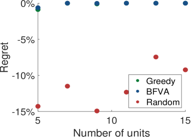
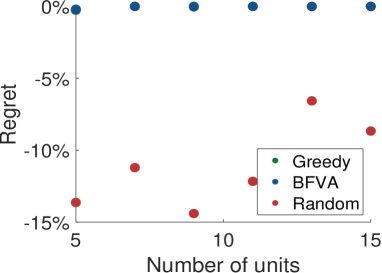
Figure 1: Comparison between the greedy algorithm and random allocation for the parameter set $1$ (Left: density $=0.3$ and Right: density $=0.6$)

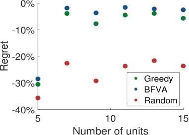
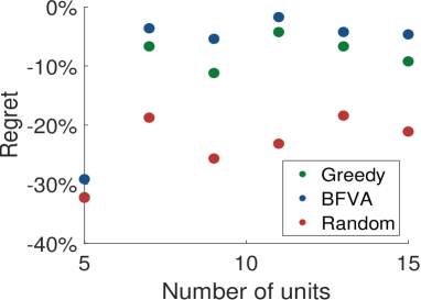
Figure 2: Comparison between the greedy algorithm and random allocation for the parameter set $2$ (Left: density $=0.3$ and Right: density $=0.6$)

4.2 Large Network

We now extend our simulation exercise to large network settings where $N=50,100$ or $150$. As previously mentioned, we can neither search over all possible allocation vectors nor compute the joint distribution over all possible vectors in a large network setting. To deal with these two problems, we first choose a baseline assignment rule – the No treatment rule – with which to compare the allocation rules that we compute. We evaluate the additional average welfare that we gain by providing treatment relative to the No treatment rule, rather than relative to the optimal assignment rule as we did for the small network setting. In Table 3, we summarize the average welfare for treatment assignment rules corresponding to greedy targeting, random allocation, and No treatment. Second, we use Gibbs sampling to approximate the joint distribution (Eq.9), iterating $10,000$ times (burning period equal to $5,000$) for each class of treatment rule.

Using Gibbs sampling, however, is not necessarily a feasible method to evaluate random allocation (and more generally) in a large network given its slow convergence. In the exercise, we use $10$ random networks and $10$ random draws, which takes approximately $30$ hours to compute a result for random allocation. In contrast, it takes only $20$ seconds to obtain a result for random allocation using variational approximation.

In Table 3, we compare the welfare delivered by Gibbs sampling with that delivered by variational approximation for the three aforementioned classes of treatment assignment rules. All the results in Table 3 are computed across $100$ random networks, using the average of $10$ random draws for random allocation, and with the capacity constraint set at $0.3N$. Table 3 indicates that variational approximation constitutes a good approximation of the Gibbs distribution (Eq.9) under Assumption 5. This provides strong evidence in favour of using the variational approximation in our algorithm.

Table 3 indicates that using our greedy algorithm leads to an increase in welfare of approximately $10\%$ as compared with random allocation. Relative to No treatment, our greedy algorithm performs $37\%\sim 55\%$ better than the random allocation. This result is robust to the network density. This suggests that the welfare gain from using our greedy algorithm carries over to the large network setting.

	Average Welfare with MCMC			Average Welfare with VA
Allocation Rule	$N=50$	$N=100$	$N=150$	$N=50$	$N=100$	$N=150$
Density $=0.3$
greedy algorithm	$0.186$	$0.186$	$0.186$	$0.186$	$0.186$	$0.186$
	($<0.01$)	($<0.01$)	($<0.01$)	($<0.01$)	($<0.01$)	($<0.01$)
Random allocation	$0.166$	$0.170$	$0.170$	$0.164$	$0.170$	$0.169$
	($<0.01$)	($<0.01$)	($<0.01$)	($<0.01$)	($<0.01$)	($<0.01$)
No treatment rule	$0.126$	$0.127$	$0.127$	$0.126$	$0.127$	$0.127$
	($<0.01$)	($<0.01$)	($<0.01$)	($<0.01$)	($<0.01$)	($<0.01$)
Density $=0.6$
greedy algorithm	$0.194$	$0.193$	$0.193$	$0.194$	$0.193$	$0.193$
	($<0.01$)	($<0.01$)	($<0.01$)	($<0.01$)	($<0.01$)	($<0.01$)
Random allocation	$0.173$	$0.178$	$0.178$	$0.172$	$0.178$	$0.178$
	($<0.01$)	($<0.01$)	($<0.01$)	($<0.01$)	($<0.01$)	($<0.01$)
No treatment rule	$0.128$	$0.129$	$0.129$	$0.127$	$0.129$	$0.129$
	($<0.01$)	($<0.01$)	($<0.01$)	($<0.01$)	($<0.01$)	($<0.01$)

Table 3: Comparison between the average welfare computed using Gibbs sampling and variational approximation for parameter set $1$

	Average Welfare with MCMC			Average Welfare with VA
Allocation Rule	$N=50$	$N=100$	$N=150$	$N=50$	$N=100$	$N=150$
Density $=0.3$
greedy algorithm	$0.227$	$0.218$	$0.215$	$0.237$	$0.228$	$0.225$
	($<0.01$)	($<0.01$)	($<0.01$)	($<0.01$)	($<0.01$)	($<0.01$)
Random allocation	$0.201$	$0.203$	$0.203$	$0.209$	$0.214$	$0.213$
	($<0.01$)	($<0.01$)	($<0.01$)	($<0.01$)	($<0.01$)	($<0.01$)
No treatment rule	$0.143$	$0.143$	$0.143$	$0.149$	$0.150$	$0.149$
	($<0.01$)	($<0.01$)	($<0.01$)	($<0.01$)	($<0.01$)	($<0.01$)
Density $=0.6$
greedy algorithm	$0.317$	$0.305$	$0.299$	$0.346$	$0.343$	$0.339$
	($<0.01$)	($<0.01$)	($<0.01$)	($<0.01$)	($<0.01$)	($<0.01$)
Random allocation	$0.287$	$0.293$	$0.292$	$0.321$	$0.334$	$0.333$
	($<0.01$)	($<0.01$)	($<0.01$)	($<0.01$)	($<0.01$)	($<0.01$)
No treatment rule	$0.171$	$0.171$	$0.170$	$0.207$	$0.208$	$0.208$
	($<0.01$)	($<0.01$)	($<0.01$)	($<0.01$)	($<0.01$)	($<0.01$)

Table 4: Comparison between the average welfare computed using Gibbs sampling and variational approximation for parameter set $2$

5 Empirical Application

We illustrate our proposed method using the dataset of Banerjee et al. (2013), which examines take-up of a microfinance initiative in India. A detailed description of the study can be found in the original paper. This study features 43 villages in Karnataka that participated in a newly available microfinance loan program. Bharatha Swamukti Samsthe (BSS)—an Indian non-governmental microfinance institution administering the initiative—provided information about the availability of microfinance and program details (the treatment) to individuals that they identified as ‘leaders’ (e.g., teachers, shopkeepers, savings group leaders, etc.) so as to maximize the number of households that chose to adopt the microfinance product. The data provide network information at the household level (network data is available across 12 dimensions, including financial and medical links, social activity, and known family members) for each village. We use all available households characteristics that are available in the dataset (quality of access to electricity, quality of latrines, number of beds, number of rooms, the number of beds per capita, and the number of rooms per capita) as covariates. The program started in 2007, and the survey for microfinance adoption was finished in early 2011. We treat each household’s choice about whether to purchase microfinance or not as observations drawn from a stationary distribution of the sequential game.

The most common occupations in these villages are in agriculture, sericulture, and dairy production (Banerjee et al., 2013). In addition, these villages had almost no exposure to microfinance institutions and other types of credit before this program. Our target in this application is to maximize the participation rate of microfinance (4 years after program assignment) given a capacity constraint on treatment (i.e., Eq.17); we set our capacity constraint equal to the number of households that BSS contacted in the original study. In the previous sections, we have assumed that the parameters $\boldsymbol{\theta}$ are given; here, we must estimate them. We estimate the parameters of our utility function for each village using Markov Chain Monte Carlo Maximum Likelihood (Snijders et al., 2002). For each iteration of the procedure, we set the number of draws in the Gibbs sampling procedure equal to $200N^{2}$. In addition, we choose $m(X_{i},X_{j})=\frac{1}{1+|X_{i}-X_{j}|}$, which is a monotonically decreasing function in the distance between $X_{i}$ and $X_{j}$. We also note that each household is connected to approximately $10$ others on average across all of the $43$ villages. Comparing this with the total number of households in each village (there are between $107$ and $341$ households in each village), we find that the household network in each village is a sparse network. We, therefore, choose $A_{N}=1$ in this application.

As an additional check, we compare the average probability of purchasing microfinance in each village—an additional statistic that we observe but that we do not use in our estimation—with the equivalent statistic that we obtain from our MCMC-MLE estimates. We refer to the sample average as the Empirical Average and to the estimated probability as the Welfare under Original Allocation. We provide standard errors for the Empirical Average, which we calculate using network HAC estimation (Leung (2019); and Kojevnikov et al. (2021)). We compute the Welfare under Original Allocation by substituting the estimated parameters and the original treatment allocation rule (used by BSS) into our model. To further evaluate the performance of our proposed method, we randomly draw 100 treatment allocations that satisfy the capacity constraint in each village, and calculate the probability of purchasing microfinance for each allocation. We refer to the average probability over these draws as the Welfare under Random Allocation. We then implement our proposed method with the estimated parameters to find the optimal treatment allocation rule. We refer to the share of households adopting microfinance according to the optimal treatment allocation and our model as the Welfare under our Greedy Allocation. Table 5 records these statistics for the $43$ villages in the dataset, with the final column comparing the Welfare under our Greedy Allocation with the Welfare under Original Allocation.

First, we assert that the estimated average share of households who adopt microfinance under the MCMC-MLE estimates fits the data well for all $43$ villages. We also find that the HAC standard error for the empirical average tends to be large, since there are relatively few households in each village, and this noise is a possible explanation for the large differences between the estimated share of households purchasing microfinance and the empirical average in some villages. Second, we find that random allocation delivers a comparable level of welfare to the original treatment allocation. This result is indicative that the leaders that BSS selected were not particularly effective in encouraging take-up by other households. Third, we find that our proposed method compares favourably to the method that is implemented in Banerjee et al. (2013), yielding a treatment allocation that attains a higher welfare-level. As shown in Table 5, the welfare gain is positive for all $43$ villages (exceeding $100\%$ in some villages). This indicates that if the specification of the sequential network game is correct in the context of the current application, individualized treatment allocation that takes into account network spillovers can generate large welfare gains—something that indicates that the network structure matters. Existing empirical work around social networks has not quantified the welfare gain from individualized treatment allocation under spillovers due to a lack of feasible procedures to obtain an optimal individualized assignment policy. In contrast, we uncover evidence of the welfare gains that can be realised by exploiting network spillovers. Fourth, we find many villages fail to satisfy Assumption 5 and Assumption 6, which are sufficient conditions for the performance guarantee to hold. Table 5, nevertheless, shows that our proposed method attains a higher welfare-level than the benchmark across all villages.

We note that Akbarpour et al. (2020) argues that the optimal treatment allocation rule under a capacity constraint may lose any advantage that it enjoys over random allocation if the capacity constraint is even slightly relaxed by a few additional households. The objective in that paper, however, is to maximize information diffusion in the context of a large network asymptotic. This is distinct from our target. We focus on the proportion of households that purchase microfinance in equilibrium. Spillover effects for product purchase are distinct from those for information diffusion both in mechanism and in intuition. In particular, we emphasize that in our setting it matters who households receive their information from and how this affects their purchase decision, rather than simply whether they are informed. We additionally note that the condition on the spillover effects that is maintained in the analysis of Akbarpour et al. (2020) becomes more restrictive when spillover effects are heterogeneous.

	Empirical Average	Welfare under Original Allocation	Welfare under Random Allocation	Welfare under Our Greedy Allocation	Welfare Gain
Village 1	$0.240$ ($0.332$)	$0.249$	$0.248$	$0.296$	$18.75\%$
Village 2	$0.146$ ($0.285$)	$0.188$	$0.195$	$0.216$	$16.81\%$
Village 3	$0.140$ ($0.378$)	$0.163$	$0.166$	$0.282$	$75.52\%$
Village 4	$0.077$ ($0.361$)	$0.101$	$0.106$	$0.173$	$72.01\%$
Village 5	$0.234$ ($0.294$)	$0.242$	$0.232$	$0.305$	$26.18\%$
Village 6	$0.184$ ($0.358$)	$0.156$	$0.162$	$0.279$	$78.57\%$
Village 7	$0.295$ ($0.485$)	$0.432$	$0.488$	$0.610$	$41.25\%$
Village 8	$0.118$ ($0.340$)	$0.130$	$0.146$	$0.216$	$66.68\%$
Village 9	$0.205$ ($0.421$)	$0.199$	$0.215$	$0.297$	$49.81\%$
Village 10	$0.356$ ($0.485$)	$0.364$	$0.405$	$0.482$	$32.18\%$
Village 11	$0.451$ ($0.645$)	$0.467$	$0.475$	$0.515$	$10.30\%$
Village 12	$0.153$ ($0.372$)	$0.153$	$0.150$	$0.176$	$14.66\%$
Village 13	$0.190$ ($0.269$)	$0.192$	$0.194$	$0.223$	$16.01\%$
Village 14	$0.169$ ($0.466$)	$0.188$	$0.202$	$0.277$	$47.82\%$
Village 15	$0.267$ ($0.332$)	$0.283$	$0.297$	$0.325$	$14.89\%$
Village 16	$0.354$ ($0.487$)	$0.346$	$0.343$	$0.414$	$19.82\%$
Village 17	$0.185$ ($0.431$)	$0.281$	$0.283$	$0.314$	$12.09\%$
Village 18	$0.186$ ($0.380$)	$0.203$	$0.201$	$0.245$	$20.82\%$
Village 19	$0.078$ ($0.273$)	$0.088$	$0.088$	$0.097$	$9.82\%$
Village 20	$0.193$ ($0.359$)	$0.200$	$0.190$	$0.328$	$64.10\%$
Village 21	$0.347$ ($0.505$)	$0.377$	$0.369$	$0.473$	$25.45\%$
Village 22	$0.245$ ($0.583$)	$0.245$	$0.239$	$0.282$	$15.09\%$
Village 23	$0.209$ ($0.397$)	$0.258$	$0.271$	$0.382$	$47.89\%$
Village 24	$0.235$ ($0.468$)	$0.250$	$0.235$	$0.299$	$21.64\%$
Village 25	$0.229$ ($0.275$)	$0.213$	$0.231$	$0.312$	$46.31\%$
Village 26	$0.187$ ($0.473$)	$0.218$	$0.225$	$0.314$	$43.95\%$
Village 27	$0.094$ ($0.283$)	$0.088$	$0.088$	$0.129$	$45.76\%$
Village 28	$0.123$ ($0.444$)	$0.104$	$0.112$	$0.186$	$79.24\%$
Village 29	$0.101$ ($0.282$)	$0.117$	$0.113$	$0.175$	$49.57\%$
Village 30	$0.110$ ($0.727$)	$0.174$	$0.179$	$0.203$	$16.75\%$
Village 31	$0.153$ ($0.328$)	$0.196$	$0.187$	$0.304$	$54.79\%$
Village 32	$0.084$ ($0.263$)	$0.091$	$0.086$	$0.216$	$137.46\%$
Village 33	$0.150$ ($0.438$)	$0.143$	$0.135$	$0.203$	$41.61\%$
Village 34	$0.177$ ($0.472$)	$0.230$	$0.229$	$0.274$	$19.16\%$
Village 35	$0.109$ ($0.331$)	$0.115$	$0.112$	$0.150$	$30.67\%$
Village 36	$0.167$ ($0.339$)	$0.166$	$0.177$	$0.238$	$43.57\%$
Village 37	$0.298$ ($0.532$)	$0.346$	$0.346$	$0.410$	$18.62\%$
Village 38	$0.147$ ($0.339$)	$0.215$	$0.205$	$0.251$	$16.44\%$
Village 39	$0.211$ ($0.357$)	$0.222$	$0.210$	$0.267$	$20.34\%$
Village 40	$0.164$ ($0.550$)	$0.170$	$0.179$	$0.310$	$81.97\%$
Village 41	$0.160$ ($0.513$)	$0.154$	$0.116$	$0.217$	$40.99\%$
Village 42	$0.177$ ($0.376$)	$0.167$	$0.194$	$0.2278$	$66.38\%$
Village 43	$0.238$ ($0.466$)	$0.181$	$0.202$	$0.326$	$80.82\%$

Table 5: Comparison using $43$ Indian villages microfinance data from Banerjee et al. (2013)

6 Conclusion

In this work, we have introduced a novel method to obtain individualized treatment allocation rules that maximize the equilibrium welfare in sequential network games. We have considered settings where the stationary joint distribution of outcomes follows a Gibbs distribution. To handle the analytical and computational challenge of analyzing the Gibbs distribution, we use variational approximation and maximize the approximated welfare criterion using a greedy maximization algorithm over treatment allocations. We have obtained bounds on the approximation error of the variational approximation and of the greedy maximization in terms of the equilibrium welfare. Moreover, we derive an upper bound on the convergence rate of the welfare regret bound. Using simulation, we have shown that our greedy algorithm performs as well as the globally optimal treatment allocation in a small network setting. In a large network setting with a given specification of parameter values, our greedy algorithm dominates random allocation and leads to a welfare improvement of around $50\%$ compared with No treatment. We then apply our method to the Indian microfinance date (Banerjee et al., 2013). We find our method outperforms both the original allocation and random allocation across all the villages. The average welfare gain is around $40\%$.

We suggest that several questions remain open and that there are several ways in which our work can be extended. First, we have not considered parameter estimation in this work. A relevant question is how to incorporate the uncertainty from parameter estimation into our analysis of regret. In addition, we may want to perform inference for the welfare at the obtained assignment rule, taking into account the uncertainty of parameter estimates and a potential winner’s bias (Andrews et al., 2020). Second, to validate the iteration method for computing the variational approximation, we rely on assumptions on the spillover effect to guarantee convergence to an optimal variational approximation. Relaxing this assumption to allow for unconstrained parameter values remains a topic for future research. Third, we have used a naive mean field method in this work. As is mentioned in Wainwright et al. (2008), using a structural mean field method can improve the performance of an approximation and can lead to better welfare performance.

Appendix A Lemma and Proposition

A.1 Preliminary Lemma

In this section, we collect various lemmata that we use to prove our main results.

Lemma A.1.

For any $\tau>0$, there is a finite set of $N\times 1$ vectors $\mathcal{W}(\tau)$ such that

$$|\mathcal{W}(\tau)|\leq 2^{N},$$ (49)

and for any $N\times 1$ vector $M$ with entries in $\{0,1\}$, there exists a $W\in\mathcal{W}(\tau)$ such that

$$\sum_{i}(M_{i}-W_{i})^{2}\leq\tau^{2}.$$ (50)

Proof.

Since all the entries of $M$ in $\{0,1\}$, $M$ must be a vertex of the N-dimensional unit hypercube $[0,1]^{N}$. As such, we let $\mathcal{W}$ be the collection of all vertices of the N-dimensional unit hypercube. For any $M$, we can always find an element in $\mathcal{W}$ such that:

$$\sum_{i}(M_{i}-W_{i})^{2}=0\leq\tau^{2}.$$ (51)

Then $|\mathcal{W}(\tau)|=2^{N}$. ∎

For completeness, we present the statement of the Banach fixed-point theorem.

Theorem A.1.

Banach Fixed-Point Theorem: Let $(X,d)$ be a non-empty complete metric space with a contraction mapping $T\mathrel{\mathop{\mathchar 58\relax}}X\rightarrow X$. Then T admits a unique fixed-point $x^{*}$.

Lemma A.2.

Suppose Assumptions 1 to 6 hold. Let $R\subset\mathcal{N}$ be a treatment allocation set, $R=\{i\in\mathcal{N}\mathrel{\mathop{\mathchar 58\relax}}d_{i}=1\}$ such that $\mathcal{N}\setminus R\neq\emptyset$. Given $k\in\mathcal{N}\setminus R$, let $\tilde{\mu}_{i}$, $i=1,\dots,N$, be a solution of the first-order conditions of Eq.31 when the treatment allocation set is $R\cup\{k\}$ and $\tilde{\mu}_{i}^{\prime}$, $i=1,\dots,N$, be a solution of Eq.31 when the treatment allocation set is $R$, i.e.,

$$\tilde{\mu}_{i}=\Lambda\big{(}\theta_{0}+\theta_{1}d_{i}+X_{i}^{\prime}(\theta_{2}+\theta_{3}d_{i})+A_{N}\theta_{5}\sum_{j\neq i}m_{ij}G_{ij}\tilde{\mu}_{j}+A_{N}\sum_{\begin{subarray}{c}j\neq i\\ j\in R\end{subarray}}m_{ij}G_{ij}(\theta_{4}+\theta_{6}d_{i}\tilde{\mu}_{j})+\mathcal{M}_{ik}(\tilde{\mu})\big{)},$$ (52)

$$\tilde{\mu}_{i}^{\prime}=\Lambda\big{(}\theta_{0}+\theta_{1}d_{i}+X_{i}^{\prime}(\theta_{2}+\theta_{3}d_{i})+A_{N}\theta_{5}\sum_{j\neq i}m_{ij}G_{ij}\tilde{\mu}_{j}^{\prime}+A_{N}\sum_{\begin{subarray}{c}j\neq i\\ j\in R\end{subarray}}m_{ij}G_{ij}(\theta_{4}+\theta_{6}d_{i}\tilde{\mu}_{j}^{\prime})\big{)},$$ (53)

where $\mathcal{M}_{ik}\mathrel{\mathop{\mathchar 58\relax}}[0,1]^{N}\to\mathbb{R}_{+}$ is defined by

$$\mathcal{M}_{ik}(\mu)=A_{N}m_{ik}G_{ik}(\theta_{4}+\theta_{6}d_{i}\mu_{k})+\mathbbm{1}\{i=k\}(X_{i}^{\prime}\theta_{3}+A_{N}\sum_{j\in R}\theta_{6}m_{ij}G_{ij}\mu_{j}).$$ (54)

Then, $\tilde{\mu}_{i}\geq\tilde{\mu}_{i}^{\prime}$ holds for all $i\in\mathcal{N}$ at any $\mathcal{X}\in\mathbb{R}^{N\times k}$ and $G\in\{0,1\}^{N\times N}$.

Proof.

Let us define $\tilde{\mu}$ as a vector with elements $\{\tilde{\mu}_{i}\}_{i=1}^{N}$ and $\tilde{\mu}^{\prime}$ as a vector with elements $\{\tilde{\mu}_{i}^{\prime}\}_{i=1}^{N}$. By the assumption that $\theta_{3},\theta_{4},\theta_{6}\geq 0$, $\mathcal{M}_{ik}$ is non-negative for all $i\in\mathcal{N}$. We define

$$\tilde{\mu}_{i}^{1}=\Lambda\big{(}\theta_{0}+\theta_{1}d_{i}+X_{i}^{\prime}(\theta_{2}+\theta_{3}d_{i})+A_{N}\theta_{5}\sum_{j\neq i}m_{ij}G_{ij}\tilde{\mu}_{j}^{\prime}+A_{N}\sum_{\begin{subarray}{c}j\neq i\\ j\in R\end{subarray}}m_{ij}G_{ij}(\theta_{4}+\theta_{6}d_{i}\tilde{\mu}_{j}^{\prime})+\mathcal{M}_{ik}(\tilde{\mu}^{\prime})\big{)},$$ (55)

for all $i\in\mathcal{N}$, where $\tilde{\mu}^{1}_{i}\geq\tilde{\mu}_{i}^{\prime}$. Then, we use $\tilde{\mu}^{1}$ to generate $\tilde{\mu}^{2}$:

$$\tilde{\mu}_{i}^{2}=\Lambda\big{(}\theta_{0}+\theta_{1}d_{i}+X_{i}^{\prime}(\theta_{2}+\theta_{3}d_{i})+A_{N}\theta_{5}\sum_{j\neq i}m_{ij}G_{ij}\tilde{\mu}_{j}^{1}+A_{N}\sum_{\begin{subarray}{c}j\neq i\\ j\in R\end{subarray}}m_{ij}G_{ij}(\theta_{4}+\theta_{6}d_{i}\tilde{\mu}_{j}^{1})+\mathcal{M}_{ik}(\tilde{\mu}^{1})\big{)},$$ (56)

for all $i\in\mathcal{N}$, where $\tilde{\mu}^{2}_{i}\geq\tilde{\mu}_{i}^{1}$. We iterate the above process until it converges. If this iteration is a contraction mapping, we can guarantee convergence to $\tilde{\mu}$, which is a unique equilibrium (by Theorem A.1). We denote this iteration process as $\{\tilde{\mu}^{t}\}_{t=1}^{\mathcal{T}}$ and show that the above mapping $T\mathrel{\mathop{\mathchar 58\relax}}[0,1]^{N}\rightarrow[0,1]^{N}$ is a contraction mapping; we equate the distance metric with the $\ell_{1}$-distance. For any $t\geq 1$,

$$d(T(\tilde{\mu}^{t}),T(\tilde{\mu}^{s}))=\sum_{i=1}^{N}\big{|}\tilde{\mu}_{i}^{t+1}-\tilde{\mu}_{i}^{s+1}\big{|},$$ (57)

$$d(\tilde{\mu}^{t},\tilde{\mu}^{s})=\sum_{i=1}^{N}\big{|}\tilde{\mu}_{i}^{t}-\tilde{\mu}_{i}^{s}\big{|}.$$ (58)

First, we know that $\Lambda(\cdot)$ is a sigmoid function. Hence, its steepest slope is 0.25.

$$\begin{split}\tilde{\mu}^{t+1}_{i}-\tilde{\mu}^{s+1}_{i}&\leq 0.25A_{N}\sum_{j\neq i}(\theta_{5}+\theta_{6}d_{i})m_{ij}G_{ij}(\tilde{\mu}_{j}^{t}-\tilde{\mu}_{j}^{s})\\ &(\text{By Multivariate Mean Value Theorem})\\ &\leq 0.25A_{N}\overline{m}(\theta_{5}+\theta_{6})\sum_{j\neq i}G_{ij}(\tilde{\mu}_{j}^{t}-\tilde{\mu}_{j}^{s}\big{)}\\ &\leq 0.25A_{N}\overline{m}(\theta_{5}+\theta_{6})\sum_{j\neq i}G_{ij}|\tilde{\mu}_{j}^{t}-\tilde{\mu}_{j}^{s}\big{|}.\end{split}$$ (59)

Therefore,

$$\begin{split}\big{|}\tilde{\mu}^{t+1}_{i}-\tilde{\mu}^{s+1}_{i}\big{|}&\leq\frac{\overline{m}A_{N}(\theta_{5}+\theta_{6})}{4}\sum_{j\neq i}G_{ij}|\tilde{\mu}_{j}^{t}-\tilde{\mu}_{j}^{s}\big{|}.\end{split}$$ (60)

Hence,

$$\begin{split}\sum_{i=1}^{N}\big{|}\tilde{\mu}^{t+1}_{i}-\tilde{\mu}^{s+1}_{i}\big{|}&\leq\frac{\overline{m}A_{N}(\theta_{5}+\theta_{6})}{4}\sum_{i=1}^{N}\sum_{j\neq i}G_{ij}|\tilde{\mu}_{j}^{t}-\tilde{\mu}_{j}^{s}\big{|}\\ &\leq\frac{\overline{m}A_{N}(\theta_{5}+\theta_{6})\overline{N}}{4}\sum_{i=1}^{N}\big{|}\tilde{\mu}_{i}^{t}-\tilde{\mu}_{i}^{s}\big{|}.\end{split}$$ (61)

By assuming $\overline{m}A_{N}(\theta_{5}+\theta_{6})\overline{N}\leq 4$, we can show that $T$ is a contraction mapping. In addition, since $\tilde{\mu}^{t}\in[0,1]$ for all $t\geq 1$, the metric space $(\tilde{\mu},d)$ is a complete metric space. By Theorem A.1, $\{\tilde{\mu}^{\prime},\tilde{\mu}^{1},...\}$ converges to $\tilde{\mu}$. Since $\mathcal{M}_{ik}\in[0,+\infty)$ for all $i\in\mathcal{N}$, this result applies for any $\mathcal{M}_{ik}$. We conclude that $\tilde{\mu}_{i}\geq\tilde{\mu}_{i}^{\mathcal{T}-1}\geq\cdots\geq\tilde{\mu}_{i}^{\prime},\forall i\in\mathcal{N}\setminus\{k\}$. ∎

Lemma A.3.

Under Assumptions 1 to 7, the upper bound on the curvature $\xi^{up}$ and the lower bound on the submodularity ratio $\gamma^{low}$ is given by:

$$\xi\leq\xi^{up}=1-\zeta\in(0,1),$$ (62)

$$\gamma\geq\gamma^{low}=\zeta\in(0,1),$$ (63)

where

$$\zeta=\frac{1}{N}\min\{\Lambda^{\prime}\big{(}\theta_{0}+\underline{X^{\prime}\theta_{2}}\big{)},\Lambda^{\prime}\big{(}\theta_{0}+\theta_{1}+\overline{X^{\prime}\theta_{2}}+\overline{X^{\prime}\theta_{3}}+A_{N}(\theta_{4}+\theta_{5}+\theta_{6})\overline{m}\overline{N}\big{)}\}\big{(}A_{N}\theta_{4}\underline{N}\cdot\underline{m}+\theta_{1}\big{)},$$ (64)

and $\underline{X^{\prime}\theta_{2}}=\min_{i\in\mathcal{N}}X_{i}^{\prime}\theta_{2}$, $\overline{X^{\prime}\theta_{2}}=\max_{i\in\mathcal{N}}X_{i}^{\prime}\theta_{2}$, $\overline{X^{\prime}\theta_{3}}=\operatorname*{arg\,max}_{i\in\mathcal{N}}X_{i}^{\prime}\theta_{3}$.

Proof.

Curvature:
The curvature is defined as the smallest value of $\xi$ such that

$$\tilde{W}(R\cup\{k\})-\tilde{W}(R)\geq(1-\xi)[\tilde{W}(S\cup\{k\})-\tilde{W}(S)]\quad\forall S\subseteq R\subseteq\mathcal{N},\forall k\in\mathcal{N}\setminus R.$$ (65)

As a consequence,

$$\xi=\max_{S\subseteq R\subset\mathcal{N},k\in\mathcal{N}\setminus R}1-\frac{\tilde{W}(R\cup\{k\})-\tilde{W}(R)}{\tilde{W}(S\cup\{k\})-\tilde{W}(S)}.$$ (66)

We first denote $\tilde{W}_{i}(\mathcal{D})$ as:

$$\begin{split}\tilde{W}_{i}(\mathcal{D})&\coloneqq\mathbbm{1}_{\{i\in\mathcal{D}\}}\Lambda\big{[}\theta_{0}+\theta_{1}+X_{i}^{\prime}(\theta_{2}+\theta_{3})+A_{N}\theta_{5}\sum_{\begin{subarray}{c}j\neq i\\ j\in\mathcal{N}\end{subarray}}m_{ij}G_{ij}\tilde{\mu}_{j}+A_{N}\sum_{\begin{subarray}{c}j\neq i\\ j\in\mathcal{D}\end{subarray}}m_{ij}G_{ij}(\theta_{4}+\theta_{6}\tilde{\mu}_{j})\big{]}\\ &\quad+\mathbbm{1}_{\{k\in\mathcal{N}\setminus\mathcal{D}\}}\Lambda\big{[}\theta_{0}+X_{k}^{\prime}\theta_{2}+A_{N}\theta_{4}\sum_{\ell\in\mathcal{D}}m_{k\ell}G_{k\ell}+A_{N}\theta_{5}\sum_{\begin{subarray}{c}\ell\neq k\\ \ell\in\mathcal{N}\end{subarray}}m_{k\ell}G_{k\ell}\tilde{\mu}_{\ell}\big{]}.\end{split}$$ (67)

We can upper bound the denominator in Eq.66 by:

$$\begin{split}\tilde{W}(S\cup\{k\})-\tilde{W}(S)&=\sum_{i=1}^{N}\tilde{W}_{i}(S\cup\{k\})-\tilde{W}_{i}(S)\leq N,\end{split}$$ (68)

A lower bound on the numerator in Eq.66 is:

$$\Delta F\doteq\tilde{W}(R\cup\{k\})-\tilde{W}(R)\quad\forall k\in\mathcal{N},R\subseteq\mathcal{N}.$$ (69)

Then we define $\xi^{up}$ as:

$$\xi^{up}\equiv 1-\frac{\Delta F}{N}\geq\xi.$$ (70)

Let $\tilde{\mu}$ denote the solution of Eq.29 with $d_{i}=1$ for $i\in R\cup\{k\}$ and $\tilde{\mu}^{\prime}$ denote the solution of Eq.29 with $d_{i}=1$ for $i\in R$. We first rewrite $\tilde{W}(R\cup\{k\})-\tilde{W}(R)$ with a view to deriving a lower bound. To do so, we define

$$\overline{\phi}_{i}(\mu)\coloneqq\theta_{0}+\theta_{1}+X_{i}^{\prime}(\theta_{2}+\theta_{3})+A_{N}\theta_{5}\sum_{j\neq i}m_{ij}G_{ij}\mu_{j}+A_{N}\sum_{\begin{subarray}{c}j\neq i\\ j\in R\end{subarray}}m_{ij}G_{ij}(\theta_{4}+\theta_{6}\mu_{j})+A_{N}m_{ik}G_{ik}(\theta_{4}+\theta_{6}\mu_{k});$$ (71)

$$\underline{\phi}_{i}(\mu)\coloneqq\theta_{0}+\theta_{1}+X_{i}^{\prime}(\theta_{2}+\theta_{3})+A_{N}\theta_{5}\sum_{j\neq i}m_{ij}G_{ij}\mu_{j}+A_{N}\sum_{\begin{subarray}{c}j\neq i\\ j\in R\end{subarray}}m_{ij}G_{ij}(\theta_{4}+\theta_{6}\mu_{j});$$ (72)

$$\overline{\varphi}_{c}(\mu)\coloneqq\theta_{0}+X_{c}^{\prime}\theta_{2}+A_{N}\theta_{5}\sum_{b\neq c}G_{cb}m_{bc}\mu_{b}+A_{N}\theta_{4}\sum_{\begin{subarray}{c}z\in R\end{subarray}}m_{cz}G_{cz}+A_{N}\theta_{4}m_{ck}G_{ck};$$ (73)

$$\underline{\varphi}_{c}(\mu)\coloneqq\theta_{0}+X_{c}^{\prime}\theta_{2}+A_{N}\theta_{5}\sum_{b\neq c}G_{cb}m_{bc}\mu_{b}+A_{N}\theta_{4}\sum_{\begin{subarray}{c}z\in R\end{subarray}}m_{cz}G_{cz};$$ (74)

$$\overline{\psi}_{k}(\mu)\coloneqq\theta_{0}+\theta_{1}+X_{k}^{\prime}(\theta_{2}+\theta_{3})+A_{N}\theta_{5}\sum_{e\neq k}m_{ke}G_{ke}\mu_{e}+A_{N}\sum_{\begin{subarray}{c}l\in R\end{subarray}}m_{kl}G_{kl}(\theta_{4}+\theta_{6}\mu_{l});$$ (75)

$$\underline{\psi}_{k}(\mu)\coloneqq\theta_{0}+X_{k}^{\prime}\theta_{2}+A_{N}\theta_{5}\sum_{e\neq k}m_{ke}G_{ke}\mu_{e}+A_{N}\theta_{4}\sum_{l\in R}m_{kl}G_{kl}$$ (76)

Then, we have

$$\begin{split}&\quad\tilde{W}(R\cup\{k\})-\tilde{W}(R)\\ &=\sum_{i\in R}\left[\Lambda\left(\overline{\phi}_{i}(\tilde{\mu})\right)-\Lambda\left(\underline{\phi}_{i}(\tilde{\mu}^{\prime})\right)\right]+\sum_{c\in\mathcal{N}\setminus R\cup\{k\}}\left[\Lambda\Big{(}\overline{\varphi}_{c}(\tilde{\mu})\Big{)}-\Lambda\left(\underline{\varphi}_{c}(\tilde{\mu}^{\prime})\right)\right]+\Lambda\left(\overline{\psi}_{k}(\tilde{\mu})\right)-\Lambda\left(\underline{\psi}_{k}(\tilde{\mu}^{\prime})\right).\end{split}$$ (77)

By Lemma A.2, we can bound the above equation from below by replacing $\tilde{\mu}_{i}^{\prime}$ with $\tilde{\mu}_{i}$ for all $i\in\mathcal{N}$. Then, Eq.77 is bounded by:

$$\begin{split}&\tilde{W}(R\cup\{k\})-\tilde{W}(R)\\ \geq&\sum_{i\in R}\left[\Lambda\left(\overline{\phi}_{i}(\tilde{\mu})\right)-\Lambda\left(\underline{\phi}_{i}(\tilde{\mu})\right)\right]+\sum_{c\in\mathcal{N}\setminus R\cup\{k\}}\left[\Lambda\Big{(}\overline{\varphi}_{c}(\tilde{\mu})\Big{)}-\Lambda\left(\underline{\varphi}_{c}(\tilde{\mu})\right)\right]+\Lambda\left(\overline{\psi}_{k}(\tilde{\mu})\right)-\Lambda\left(\underline{\psi}_{k}(\tilde{\mu})\right).\end{split}$$ (78)

Using the mean value theorem, and letting $\phi_{i}\in\left(\underline{\phi}_{i}(\tilde{\mu}),\overline{\phi}_{i}(\tilde{\mu})\right)$, $\varphi_{c}\in\left(\underline{\varphi}_{c}(\tilde{\mu}),\overline{\varphi}_{c}(\tilde{\mu})\right)$, $\psi_{k}\in\left(\underline{\psi}_{k}(\tilde{\mu}),\overline{\psi}_{k}(\tilde{\mu})\right)$, we have:

$$\begin{split}&\quad\tilde{W}(R\cup\{k\})-\tilde{W}(R)\\ &\geq\sum_{i\in R}\Lambda^{\prime}(\phi_{i})A_{N}(\theta_{4}+\theta_{6}\tilde{\mu}_{k})m_{ik}G_{ik}+\sum_{c\in\mathcal{N}\setminus R\cup\{k\}}\Lambda^{\prime}(\varphi_{c})A_{N}\theta_{4}m_{ck}G_{ck}\\ &\quad+\Lambda^{\prime}(\psi_{k})(\theta_{1}+X_{k}^{\prime}\theta_{3}+\theta_{6}A_{N}\sum_{l\in R}m_{kl}G_{kl}\tilde{\mu}_{l})\\ &\geq\sum_{i\in R}\Lambda^{\prime}(\phi_{i})A_{N}\theta_{4}m_{ik}G_{ik}+\sum_{c\in\mathcal{N}\setminus R\cup\{k\}}\Lambda^{\prime}(\varphi_{c})A_{N}\theta_{4}m_{ck}G_{ck}+\Lambda^{\prime}(\psi_{k})\theta_{1}\\ &\geq\sum_{i\in R}\underline{\Lambda^{\prime}(\phi_{i})}A_{N}\theta_{4}m_{ik}G_{ik}+\sum_{c\in\mathcal{N}\setminus R\cup\{k\}}\underline{\Lambda^{\prime}(\varphi_{c})}A_{N}\theta_{4}m_{ck}G_{ck}+\underline{\Lambda^{\prime}(\psi_{k})}\theta_{1}\\ &\geq\underline{\Lambda^{\prime}}\cdot\big{(}\sum_{i\neq k}A_{N}\theta_{4}m_{ik}G_{ik}+\theta_{1}\big{)}\\ &\geq\underline{\Lambda^{\prime}}\cdot\big{(}A_{N}\theta_{4}\underline{N}\cdot\underline{m}+\theta_{1}\big{)},\end{split}$$ (79)

where

$$\underline{\Lambda^{\prime}(\phi_{i})}=\min\{\Lambda^{\prime}(\underline{\phi}_{i}),\Lambda^{\prime}(\overline{\phi}_{i})\},$$ (80)

$$\underline{\Lambda^{\prime}(\varphi_{c})}=\min\{\Lambda^{\prime}(\underline{\varphi}_{c}),\Lambda^{\prime}(\overline{\varphi}_{c})\},$$ (81)

$$\underline{\Lambda^{\prime}(\psi_{k})}=\min\{\Lambda^{\prime}(\underline{\psi}_{k}),\Lambda^{\prime}(\overline{\psi}_{k})\},$$ (82)

$$\underline{\Lambda^{\prime}}=\min\{\Lambda^{\prime}\big{(}\theta_{0}+\underline{X^{\prime}\theta_{2}}\big{)},\Lambda^{\prime}\big{(}\theta_{0}+\theta_{1}+\overline{X^{\prime}\theta_{2}}+\overline{X^{\prime}\theta_{3}}+A_{N}(\theta_{4}+\theta_{5}+\theta_{6})\overline{m}\overline{N}\big{)}\}.$$ (83)

Then,

$$\xi^{up}=1-\frac{1}{N}\underline{\Lambda^{\prime}}\cdot\big{(}A_{N}\theta_{4}\underline{N}\cdot\underline{m}+\theta_{1}\big{)}.$$ (84)

Under Assumption 2 and 6

$$\begin{split}\theta_{1},\theta_{4},A_{N},\underline{N},\underline{m}>0\Rightarrow\big{(}A_{N}\theta_{4}\underline{N}\cdot\underline{m}+\theta_{1}\big{)}>0.\end{split}$$ (85)

In addition, we know that $\Lambda(x)$ is a logistic function, and so

$$\begin{split}&\Lambda^{\prime}\big{(}\theta_{0}+\underline{X^{\prime}\theta_{2}}\big{)}\in(0,0.25],\\ &\Lambda^{\prime}\big{(}\theta_{0}+\theta_{1}+\overline{X^{\prime}\theta_{2}}+\overline{X^{\prime}\theta_{3}}+A_{N}(\theta_{3}+\theta_{4}+\theta_{5})\overline{m}\overline{N}\big{)}\in(0,0.25].\\ \end{split}$$ (86)

Hence,

$$\begin{split}\underline{\Lambda^{\prime}}\in(0,0.25).\end{split}$$ (87)

By assuming that $\big{(}A_{N}\theta_{4}\underline{N}\cdot\underline{m}+\theta_{1}\big{)}\leq 4N$, we obtain

$$\begin{split}\underline{\Lambda^{\prime}}\cdot\big{(}A_{N}\theta_{4}\underline{N}\cdot\underline{m}+\theta_{1}\big{)}<N.\end{split}$$ (88)

We conclude that $\xi^{up}<1$. From Bian et al. (2017), $\xi$ only equal to 0 if $\tilde{W}(\mathcal{D})$ is supermodular. Since $\tilde{W}(\mathcal{D})$ is not supermodular, $\xi^{up}>\xi>0$.

Submodularity Ratio

The submodularity ratio of a non-negative set function is the largest $\gamma$ such that

$$\sum_{k\in R\setminus S}[\tilde{W}(S\cup\{k\})-\tilde{W}(S)]\geq\gamma[\tilde{W}(S\cup R)-\tilde{W}(S)],\quad\forall S,R\subseteq\mathcal{N}.$$ (89)

As a consequence,

$$\begin{split}\gamma&=\min_{S\neq R}\frac{\sum_{k\in R\setminus S}[\tilde{W}(S\cup\{k\})-\tilde{W}(S)]}{\tilde{W}(S\cup R)-\tilde{W}(S)}\\ &=\min_{S\neq R}\frac{\sum_{k\in R\setminus S}\sum_{i}[\tilde{W}_{i}(S\cup\{k\})-\tilde{W}_{i}(S)]}{\sum_{i}[\tilde{W}_{i}(S\cup R)-\tilde{W}_{i}(S)]}\end{split}$$ (90)

We can upper bound the denominator in Eq.90 by:

$$\sum_{i=1}^{N}[\tilde{W}_{i}(S\cup R)-\tilde{W}_{i}(S)]\leq N.$$ (91)

We first rewrite $\sum_{k\in R\setminus S}[\tilde{W}(S\cup\{k\})-\tilde{W}(S)]$ with a view to deriving a lower bound.

$$\begin{split}&\quad\sum_{k\in R\setminus S}\sum_{i}[\tilde{W}_{i}(S\cup\{k\})-\tilde{W}_{i}(S)]\\ &=\sum_{k\in R\setminus S}\Bigg{[}\sum_{i\in S}\Big{[}\Lambda\big{(}\theta_{0}+\theta_{1}+X_{i}^{\prime}(\theta_{2}+\theta_{3})+A_{N}\theta_{5}\sum_{j\neq i}m_{ij}G_{ij}\tilde{\mu}_{j}+A_{N}\sum_{\begin{subarray}{c}j\neq i\\ j\in S\end{subarray}}m_{ij}G_{ij}(\theta_{4}+\theta_{6}\tilde{\mu}_{j})\\ &\quad+A_{N}m_{ik}G_{ik}(\theta_{4}+\theta_{6}\tilde{\mu}_{k})\big{)}-\Lambda\big{(}\theta_{0}+\theta_{1}+X_{i}^{\prime}(\theta_{2}+\theta_{3})+A_{N}\theta_{5}\sum_{j\neq i}m_{ij}G_{ij}\tilde{\mu}_{j}^{\prime}+A_{N}\sum_{\begin{subarray}{c}j\neq i\\ j\in S\end{subarray}}m_{ij}G_{ij}(\theta_{4}+\theta_{6}\tilde{\mu}_{j}^{\prime})\big{)}\Big{]}\\ &\quad+\sum_{c\in\mathcal{N}\setminus S\cup\{k\}}\Big{[}\Lambda\big{(}\theta_{0}+X_{c}^{\prime}\theta_{2}+A_{N}\theta_{5}\sum_{b\neq c}G_{cb}m_{bc}\tilde{\mu}_{b}+A_{N}\theta_{4}\sum_{\begin{subarray}{c}z\in S\end{subarray}}m_{cz}G_{cz}+A_{N}\theta_{4}m_{ck}G_{ck}\big{)}\\ &\quad-\Lambda(\theta_{0}+X_{c}^{\prime}\theta_{2}+A_{N}\theta_{5}\sum_{b\neq c}G_{cb}m_{bc}\tilde{\mu}_{b}^{\prime}+A_{N}\theta_{4}\sum_{\begin{subarray}{c}z\in S\end{subarray}}m_{cz}G_{cz})\Big{]}\\ &\quad+\Lambda(\theta_{0}+\theta_{1}+X_{k}^{\prime}(\theta_{2}+\theta_{3})+A_{N}\theta_{5}\sum_{e\neq k}m_{ke}G_{ke}\tilde{\mu}_{e}+A_{N}\sum_{\begin{subarray}{c}l\in S\end{subarray}}m_{kl}G_{kl}(\theta_{4}+\theta_{6}\tilde{\mu}_{l}))\\ &\quad-\Lambda(\theta_{0}+X_{k}^{\prime}\theta_{2}+A_{N}\theta_{5}\sum_{e\neq k}m_{ke}G_{ke}\tilde{\mu}_{e}^{\prime}+A_{N}\theta_{4}\sum_{l\in S}m_{kl}G_{kl})\Bigg{]}.\end{split}$$ (92)

We can lower bound the numerator in Eq.90 by:

$$\begin{split}\sum_{k\in R\setminus S}\sum_{i}[\tilde{W}_{i}(S\cup\{k\})-\tilde{W}_{i}(S)]&\geq\sum_{k\in R\setminus S}\underline{\Lambda^{\prime}}\cdot\big{(}A_{N}\theta_{4}\underline{N}\cdot\underline{m}+\theta_{1}\big{)}\\ &(\text{By Eq.\ref{eqrk}})\\ &\geq\underline{\Lambda^{\prime}}\cdot\big{(}A_{N}\theta_{4}\underline{N}\cdot\underline{m}+\theta_{1}\big{)}\end{split}$$ (93)

Defining:

$$\gamma^{low}=\frac{1}{N}\underline{\Lambda^{\prime}}\cdot\big{(}A_{N}\theta_{4}\underline{N}\cdot\underline{m}+\theta_{1}\big{)},$$ (94)

the submodularity ratio can be bounded from below by:

$$\gamma\geq\gamma^{low}=1-\xi^{up}\in(0,1).$$ (95)

∎

A.2 Proof of Proposition 2.1

Under Assumptions 1 and 4, the potential function $\Phi(y,\mathcal{X},D,G;\boldsymbol{\theta})$ for $U_{i}(y,\mathcal{X},D,G;\boldsymbol{\theta})$ can be defined as:

$$\begin{split}\Phi(y,\mathcal{X},D,G;\boldsymbol{\theta})&=\sum_{i=1}^{N}\left(\theta_{0}+\theta_{1}d_{i}+X_{i}^{\prime}(\theta_{2}+\theta_{3}d_{i})+A_{N}\sum_{j=1}^{N}\theta_{4}m_{ij}G_{ij}d_{j}\right)y_{i}\\ &\quad+\frac{A_{N}}{2}\sum_{i=1}^{N}\sum_{j=1}^{N}m_{ij}G_{ij}y_{i}y_{j}(\theta_{5}+\theta_{6}d_{i}d_{j}),\end{split},$$ (96)

and our interacted decision game is a potential game.

Proof.

A potential function is a function $\Phi\mathrel{\mathop{\mathchar 58\relax}}Y\rightarrow\mathbb{R}$ such that:

$$\Phi(y_{i}=1,y_{-i},\mathcal{X},D,G)-\Phi(y_{i}=0,y_{-i},\mathcal{X},D,G)=U_{i}(y_{i}=1,y_{-i},\mathcal{X},D,G)-U_{i}(y_{i}=0,y_{-i},\mathcal{X},D,G).$$ (97)

Simple computation shows that for any $i\in\mathcal{N}$,

$$\begin{split}&\quad\Phi(y_{i}=1,y_{-i},\mathcal{X},D,G)-\Phi(y_{i}=0,y_{-i},\mathcal{X},D,G)\\ &=\theta_{0}+\theta_{1}d_{i}+X_{i}^{\prime}(\theta_{2}+\theta_{3}d_{i})+A_{N}\sum_{j=1}^{N}\theta_{4}m_{ij}G_{ij}d_{j}+A_{N}\sum_{j=1}^{N}m_{ij}G_{ij}y_{j}(\theta_{5}+\theta_{6}d_{i}d_{j})\\ &=U_{i}(y_{i}=1,y_{-i},\mathcal{X},D,G)-U_{i}(y_{i}=0,y_{-i},\mathcal{X},D,G).\end{split}$$ (98)

Therefore, $\Phi$ is the potential of our interacted decision game.

∎

A.3 Proof of Proposition 3.1

Under Assumptions 1 to 4, the optimization for $\tilde{\mu}$ has a unique maximizer and the iteration procedure of Algorithm 1 converges to this maximizer.

Proof.

To prove the existence of a unique maximizer, we need to show that two conditions are satisfied.

• The objective function is continuous and differentiable in the interior.

• The boundary point cannot be a global optimum.

Since our objective function is the sum of linear terms, quadratic functions and logarithmic functions, the first condition is trivially satisfied. To check the second condition, we need to verify that the derivative is positive at $\mu^{Q}_{i}=0$ and is negative at $\mu^{Q}_{i}=1$. The derivative is:

$$\begin{split}\frac{\partial}{\partial\mu^{Q}_{i}}\mathcal{A}(\mu^{Q},\mathcal{X},D,G)&=\theta_{0}+\theta_{1}d_{i}+X_{i}^{\prime}\theta_{2}+X_{i}^{\prime}\theta_{3}d_{i}+A_{N}\sum_{j=1}^{N}\theta_{4}m_{ij}G_{ij}d_{j}\\ &\quad+A_{N}\sum_{j=1}^{N}m_{ij}G_{ij}(\theta_{5}+\theta_{6}d_{i}d_{j})\mu^{Q}_{j}-\log(\mu^{Q}_{i})+\log(1-\mu^{Q}_{i}).\end{split}$$ (99)

When $\mu^{Q}_{i}=0$,

$$-\log(\mu^{Q}_{i})+\log(1-\mu^{Q}_{i})=-\log(0)+\log(1)=+\infty.$$ (100)

When $\mu^{Q}_{i}=1$,

$$-\log(\mu^{Q}_{i})+\log(1-\mu^{Q}_{i})=-\log(1)+\log(0)=-\infty.$$ (101)

Since all of the elements in $\theta_{0}+\theta_{1}d_{i}+X_{i}^{\prime}\theta_{2}+X_{i}^{\prime}\theta_{3}d_{i}+A_{N}\sum_{j=1}^{N}\theta_{4}m_{ij}G_{ij}d_{j}+A_{N}\sum_{j=1}^{N}m_{ij}G_{ij}(\theta_{5}+\theta_{6}d_{i}d_{j})\mu^{Q}_{j}$ are bounded,

$$\frac{\partial}{\partial\mu^{Q}_{i}}\mathcal{A}(\mu^{Q},\mathcal{X},D,G)|_{\mu^{Q}_{i}=0}=+\infty,$$ (102)

and

$$\frac{\partial}{\partial\mu^{Q}_{i}}\mathcal{A}(\mu^{Q},\mathcal{X},D,G)|_{\mu^{Q}_{i}=1}=-\infty.$$ (103)

Away from the boundary, the objective function increases. A global optimum, if it exists, then has to be in the interior. Since the objective function is continuous and differentiable, the first-order condition has to be satisfied at the global optimum. The coordinate ascent property that holds at every iterative step implies that the objective function increases at each step, which further implies that the point that the algorithm converges to cannot be a local maximum. ∎

A.4 Proof of Proposition 3.2

Under Assumptions 1 to 5, the iteration procedure in Algorithm 1 is a contraction mapping for all $i\in\mathcal{N}$, for all $\{d_{i}\}_{i=1}^{N}\in\{0,1\}^{N}$, for all $\mathcal{X}\in\mathbb{R}^{N\times k}$, and for all $G\in\{0,1\}^{N\times N}$.

Proof.

This proof is very similar to Lemma A.2. Recall the iteration in Algorithm 1:

$$\tilde{\mu}_{i}^{t+1}=\Lambda\Big{[}\theta_{0}+\theta_{1}d_{i}+X_{i}^{\prime}(\theta_{2}+\theta_{3}d_{i})+A_{N}\theta_{4}\sum\limits_{j\neq i}m_{ij}G_{ij}d_{j}+A_{N}\sum\limits_{j\neq i}m_{ij}G_{ij}(\theta_{5}+\theta_{6}d_{i}d_{j})\tilde{\mu}_{j}^{t}\Big{]}.$$ (104)

We denote this iteration process as $\{\tilde{\mu}^{t}\}_{t=1}^{\mathcal{T}}$ and show the above mapping $T\mathrel{\mathop{\mathchar 58\relax}}[0,1]^{N}\rightarrow[0,1]^{N}$ is a contraction mapping. To prove the above iteration is a contraction mapping, we use $\ell_{1}$-distance. For any $t\geq 1$,

$$d(T(\tilde{\mu}^{t}),T(\tilde{\mu}^{s}))=\sum_{i=1}^{N}\big{|}\tilde{\mu}_{i}^{t+1}-\tilde{\mu}_{i}^{s+1}\big{|},$$ (105)

$$d(\tilde{\mu}^{t},\tilde{\mu}^{s})=\sum_{i=1}^{N}\big{|}\tilde{\mu}_{i}^{t}-\tilde{\mu}_{i}^{s}\big{|}.$$ (106)

First, we know $\Lambda(\cdot)$ is a sigmoid function. Hence, its largest slope is 0.25.

$$\begin{split}\tilde{\mu}^{t+1}_{i}-\tilde{\mu}^{s+1}_{i}&\leq 0.25A_{N}\sum_{j\neq i}(\theta_{5}+\theta_{6}d_{i}d_{j})m_{ij}G_{ij}(\tilde{\mu}_{j}^{t}-\tilde{\mu}_{j}^{s})\\ &(\text{By Multivariate Mean Value Theorem})\\ &\leq 0.25A_{N}\overline{m}(|\theta_{5}|+|\theta_{6}|)\sum_{j\neq i}G_{ij}(\tilde{\mu}_{j}^{t}-\tilde{\mu}_{j}^{s}\big{)}\\ &\leq 0.25A_{N}\overline{m}(|\theta_{5}|+|\theta_{6}|)\sum_{j\neq i}G_{ij}|\tilde{\mu}_{j}^{t}-\tilde{\mu}_{j}^{s}\big{|}.\end{split}$$ (107)

Therefore,

$$\begin{split}\big{|}\tilde{\mu}^{t+1}_{i}-\tilde{\mu}^{s+1}_{i}\big{|}&\leq\frac{\overline{m}A_{N}(|\theta_{5}|+|\theta_{6}|)}{4}\sum_{j\neq i}G_{ij}|\tilde{\mu}_{j}^{t}-\tilde{\mu}_{j}^{s}\big{|}.\end{split}$$ (108)

Hence,

$$\begin{split}\sum_{i=1}^{N}\big{|}\tilde{\mu}^{t+1}_{i}-\tilde{\mu}^{s+1}_{i}\big{|}&\leq\frac{\overline{m}A_{N}(|\theta_{5}|+|\theta_{6}|)}{4}\sum_{i=1}^{N}\sum_{j\neq i}G_{ij}|\tilde{\mu}_{j}^{t}-\tilde{\mu}_{j}^{s}\big{|}\\ &\leq\frac{\overline{m}A_{N}(|\theta_{5}|+|\theta_{6}|)\overline{N}}{4}\sum_{i=1}^{N}\big{|}\tilde{\mu}_{i}^{t}-\tilde{\mu}_{i}^{s}\big{|}.\end{split}$$ (109)

Therefore, under Assumption 5, $T$ is a contraction mapping. In addition, since $\tilde{\mu}^{t}\in[0,1]$ for all $t\geq 1$, the metric space $(\tilde{\mu},d)$ is a complete metric space. By Theorem A.1, $\{\tilde{\mu}^{\prime},\tilde{\mu}^{1},...\}$ will converge to a unique fixed point, which is $\tilde{\mu}$. ∎

A.5 Proof of Lemma 3.1

Under Assumptions 1 to 6, $\tilde{W}(\mathcal{D})$ is a non-negative and non-decreasing set function.

Proof.

First, since $\tilde{W}(\mathcal{D})$ is the summation of logistic functions and the logistic function is non-negative, $\tilde{W}(\mathcal{D})$ is non-negative. Second, if we assign one more unit $z$ to $\mathcal{D}$, by Lemma A.2, for all $i\in\mathcal{N}$, $\tilde{\mu}_{i}$ is non-decreasing. $\tilde{W}(\mathcal{D})$ is, therefore, a non-decreasing set function. ∎

Appendix B Theorem

B.1 Proof of Theorem 3.1

Let $Q^{*}$ denote the independent Bernoulli distribution that solves Eq.29. Under Assumptions 1 to 4, the Kullback–Leibler divergence between $Q^{*}$ and $P$ is bounded from above by:

$$\mathbb{KL}(Q^{*}||P)\leq C_{1}A_{N}\overline{N}+C_{2}N+\mathcal{O}\left(\sqrt{A_{N}^{2}\overline{N}^{2}N}\right)+\mathcal{O}\left(\sqrt{A_{N}^{3}\overline{N}^{2}N^{2}}\right)+\mathcal{O}\left(\sqrt{A_{N}^{3}\overline{N}N^{3}}\right)+o(N),$$ (110)

where $C_{1},C_{2},C_{3},C_{4},C_{5},C_{6}$ are constants that depend only upon $\boldsymbol{\theta}$, $\overline{m}$, $\max_{1\leq i\leq N}|X_{i}^{\prime}\theta_{2}|$, and $\max_{1\leq i\leq N}|X_{i}^{\prime}\theta_{3}|$.

For completeness, we present the statement of Theorem 1.6 in Chatterjee and Dembo (2016).

Theorem B.1.

Chatterjee and Dembo (2016) Suppose that $f\mathrel{\mathop{\mathchar 58\relax}}[0,1]^{N}\rightarrow\mathbb{R}$ is twice continuously differentiable in $(0,1)^{N}$, so that $f$ and all of its first- and second-order derivatives extend continuously to the boundary. Let $\lVert f\rVert$ denote the supremum norm of $f\mathrel{\mathop{\mathchar 58\relax}}[0,1]^{N}\rightarrow\mathbb{R}$. For each $i$ and $j$, denote

$$f_{i}\mathrel{\mathop{\mathchar 58\relax}}=\frac{\partial f}{\partial x_{i}},\quad f_{ij}\mathrel{\mathop{\mathchar 58\relax}}=\frac{\partial^{2}f}{\partial x_{i}\partial x_{j}},$$ (111)

and let

$$a\mathrel{\mathop{\mathchar 58\relax}}=\lVert f\rVert,\quad b_{i}\mathrel{\mathop{\mathchar 58\relax}}=\lVert f_{i}\rVert,\quad c_{ij}\mathrel{\mathop{\mathchar 58\relax}}=\lVert f_{ij}\rVert.$$ (112)

Given $\epsilon>0$, $\mathcal{M}(\epsilon)$ is a finite subset of $\mathbb{R}^{N}$ such that for any $\tilde{\mu}\in\{0,1\}^{N}$, there exists $\eta=(\eta_{1},...,\eta_{N})\in\mathcal{M}(\epsilon)$ such that

$$\sum_{i}\Big{(}\frac{\partial f(\tilde{\mu})}{\partial\tilde{\mu}_{i}}-\eta_{i}\Big{)}^{2}\leq N\epsilon^{2}.$$ (113)

Let us define for any $\tilde{\mu}=(\tilde{\mu}_{1},...,\tilde{\mu}_{N})\in[0,1]^{N}$,

$$I(\tilde{\mu})=\sum_{i=1}^{N}\left[\tilde{\mu}_{i}\log\tilde{\mu}_{i}+(1-\tilde{\mu}_{i})\log(1-\tilde{\mu}_{i})\right].$$ (114)

Let us define

$$F=\sup_{\tilde{\mu}\in[0,1]^{N}}(f(\tilde{\mu})-I(\tilde{\mu}))+\text{lower order terms}.$$ (115)

Then for an $\epsilon>0,$

$$F\leq\sup_{\tilde{\mu}\in[0,1]^{N}}(f(\tilde{\mu})-I(\tilde{\mu}))+\textit{complexity term}+\textit{smoothness term}.$$ (116)

where

$$\textit{complexity term}=\frac{1}{4}\Big{(}n\sum_{i=1}^{N}b_{i}^{2}\Big{)}^{1/2}\epsilon+3N\epsilon+\log|\mathcal{M}(\epsilon)|,$$ (117)

and

$$\begin{split}\textit{smoothness term}&=4\Big{(}\sum_{i=1}^{N}(ac_{ii}+b_{i}^{2})+\frac{1}{4}\sum_{i,j=1}^{N}(ac_{ij}^{2}+b_{i}b_{j}c_{ij}+4b_{i}c_{ij})\Big{)}^{1/2}\\ &\quad+\frac{1}{4}\Big{(}\sum_{i=1}^{N}b_{i}^{2}\Big{)}^{1/2}\Big{(}\sum_{i=1}^{N}c_{ii}^{2}\Big{)}^{1/2}+3\sum_{i=1}^{N}c_{ii}+\log 2.\end{split}$$ (118)

Proof.

We need to apply Theorem B.1. We define $f\mathrel{\mathop{\mathchar 58\relax}}[0,1]^{N}\rightarrow\mathbb{R}$ as:

$$f(\tilde{\mu})=\sum_{i}(\theta_{0}+\theta_{1}d_{i}+X_{i}^{\prime}(\theta_{2}+\theta_{3}d_{i})+A_{N}\theta_{4}\sum\limits_{j\neq i}m_{ij}G_{ij}d_{j})\tilde{\mu}_{i}+\frac{A_{N}}{2}\sum_{i}\sum_{j}(\theta_{5}+\theta_{6}d_{i}d_{j})m_{ij}G_{ij}\tilde{\mu}_{i}\tilde{\mu}_{j}.$$ (119)

Therefore,

$$\begin{split}\lVert f\rVert&\leq\sum_{i}(|\theta_{0}|+|\theta_{1}|+|X_{i}^{\prime}\theta_{2}|+|\theta_{3}X_{i}|)+A_{N}\sum_{i}\sum_{j}|\theta_{4}m_{ij}|G_{ij}+\frac{A_{N}}{2}\sum_{i}\sum_{j}G_{ij}(|\theta_{5}m_{ij}|+|\theta_{6}m_{ij}|)\\ &\leq N(|\theta_{0}|+|\theta_{1}|+\max_{i}|X_{i}^{\prime}\theta_{2}|+\max_{i}|X_{i}^{\prime}\theta_{3}|)+\overline{m}A_{N}(|\theta_{4}|+|\theta_{5}|+|\theta_{6}|)\sum_{i}\sum_{j}G_{ij}\\ &\leq N(|\theta_{0}|+|\theta_{1}|+\max_{i}|X_{i}^{\prime}\theta_{2}|+\max_{i}|X_{i}^{\prime}\theta_{3}|)+\overline{m}A_{N}N\overline{N}(|\theta_{4}|+|\theta_{5}|+|\theta_{6}|)\\ &\eqqcolon\tilde{a}.\end{split}$$ (120)

The partial derivative of $f(\tilde{\mu})$ with respect to $\tilde{\mu}_{i}$ is:

$$\frac{\partial f(\tilde{\mu})}{\partial\tilde{\mu}_{i}}=\theta_{0}+\theta_{1}+X_{i}^{\prime}\theta_{2}+X_{i}^{\prime}\theta_{3}d_{i}+A_{N}\sum_{j\neq i}\theta_{4}m_{ij}G_{ij}d_{j}+A_{N}\sum_{j\neq i}\theta_{5}m_{ij}G_{ij}\tilde{\mu}_{j}+A_{N}\sum_{j\neq i}\theta_{6}m_{ij}G_{ij}d_{i}d_{j}\tilde{\mu}_{j}.$$ (121)

Therefore,

$$\begin{split}\lVert\nabla_{i}f(\tilde{\mu})\rVert\leq|\theta_{0}|+|\theta_{1}|+\max_{i}|X_{i}^{\prime}\theta_{2}|+\max_{i}|X_{i}^{\prime}\theta_{3}|+\overline{m}A_{N}\overline{N}(|\theta_{4}|+|\theta_{5}|+|\theta_{6}|)\eqqcolon\tilde{b}.\end{split}$$ (122)

The second partial derivative with respect to $\tilde{\mu}_{j}$ is:

$$\frac{\partial^{2}f(\tilde{\mu})}{\partial\tilde{\mu}_{i}\partial\tilde{\mu}_{j}}=A_{N}\theta_{5}m_{ij}G_{ij}+A_{N}\theta_{6}m_{ij}G_{ij}d_{i}d_{j}.$$ (123)

Therefore, for all $j\neq i$,

$$\lVert\nabla_{i}\nabla_{j}g(\tilde{\mu})\rVert\leq\overline{m}A_{N}(|\theta_{5}|+|\theta_{6}|)\eqqcolon\tilde{c},$$ (124)

with the second derivative zero if $i=j$. Next, we need to compute $|\mathcal{M}(\epsilon)|$, where $\mathcal{M}(\epsilon)$ is the finite subset of $\mathbb{R}^{N}$ such that for any $\tilde{\mu}\in\{0,1\}^{N}$, there exists $\eta=(\eta_{1},...,\eta_{N})\in\mathcal{M}(\epsilon)$ such that

$$\sum_{i}\Big{(}\frac{\partial f(\tilde{\mu})}{\partial\tilde{\mu}_{i}}-\eta_{i}\Big{)}^{2}\leq N\epsilon^{2}.$$ (125)

We note that this is requirement on the derivative at the boundary; we only need the above condition to hold when $\tilde{\mu}\in\{0,1\}^{N}$ to define $\mathcal{M}(\epsilon)$, and not more generally for $\tilde{\mu}\in(0,1)^{N}$. Recalling Eq.121 and defining $T_{1}$ and $T_{2}$ as:

$$\begin{split}T_{1}(\tilde{\mu})\coloneqq\frac{A_{N}\theta_{5}}{2}\sum_{i}\sum_{j}m_{ij}G_{ij}\tilde{\mu}_{i}\tilde{\mu}_{j},\quad T_{2}(\tilde{\mu})\coloneqq\frac{A_{N}\theta_{6}}{2}\sum_{i}\sum_{j}m_{ij}G_{ij}d_{i}d_{j}\tilde{\mu}_{i}\tilde{\mu}_{j},\end{split}$$ (126)

we state the partial derivative of $f(\tilde{\mu})$ as

$$\begin{split}\frac{\partial f(\tilde{\mu})}{\partial\tilde{\mu}_{i}}&=\theta_{0}+\theta_{1}+X_{i}^{\prime}\theta_{2}+X_{i}^{\prime}\theta_{3}d_{i}+\theta_{4}A_{N}\sum_{j}m_{ij}G_{ij}d_{j}+\frac{\partial T_{1}(\tilde{\mu})}{\partial\tilde{\mu}_{i}}+\frac{\partial T_{2}(\tilde{\mu})}{\partial\tilde{\mu}_{i}}.\end{split}$$ (127)

Let $\mathcal{M}_{1}(\epsilon)$ be the finite subset of $\mathbb{R}^{N}$ such that for any $\tilde{\mu}\in\{0,1\}^{N}$, there exists $\lambda=(\lambda_{1},...,\lambda_{N})\in\mathcal{M}_{1}(\epsilon)$ such that

$$\sum_{i}\Big{(}\frac{\partial T_{1}(\tilde{\mu})}{\partial\tilde{\mu}_{i}}-\lambda_{i}\Big{)}^{2}\leq N\epsilon^{2}.$$ (128)

Let $\mathcal{M}_{2}(\epsilon)$ be the finite subset of $\mathbb{R}^{N}$ such that for any $\tilde{\mu}\in\{0,1\}^{N}$, there exists $\vartheta=(\vartheta_{1},...,\vartheta_{N})\in\mathcal{M}_{2}(\epsilon)$ such that

$$\sum_{i}\Big{(}\frac{\partial T_{2}(\tilde{\mu})}{\partial\tilde{\mu}_{i}}-\vartheta_{i}\Big{)}^{2}\leq N\epsilon^{2}.$$ (129)

Defining $\lambda_{i}$ and $\vartheta_{i}$ for all $i\in\mathcal{N}$ to be:

$$\lambda_{i}=A_{N}\theta_{5}\sum_{j}m_{ij}G_{ij}\tilde{y}_{j},\quad\vartheta_{i}=A_{N}\theta_{6}\sum_{j}m_{ij}G_{ij}d_{i}d_{j}\tilde{v}_{j},$$ (130)

where $\tilde{y}_{j}\in\{0,1\}$ and $\tilde{v}_{j}\in\{0,1\}$ by Lemma A.1, we can then define $\mathcal{M}(\epsilon)$ as:

$$\begin{split}\mathcal{M}(\epsilon)&\mathrel{\mathop{\mathchar 58\relax}}=\Big{\{}\theta_{0}+\theta_{1}+X_{i}^{\prime}\theta_{2}+X_{i}^{\prime}\theta_{3}d_{i}+A_{N}\theta_{4}\sum_{j}m_{ij}G_{ij}d_{j}+\ell_{1}+\ell_{2}\\ &\quad\mathrel{\mathop{\mathchar 58\relax}}\ell_{1}\in\mathcal{M}_{1}\left(\frac{\epsilon}{\sqrt{2}}\right),\ell_{2}\in\mathcal{M}_{2}\left(\frac{\epsilon}{\sqrt{2}}\right),i\in\mathcal{N}\Big{\}}.\end{split}$$ (131)

Then,

$$\begin{split}\Big{(}\frac{\partial T_{1}(\tilde{\mu})}{\partial\tilde{\mu}_{i}}-\lambda_{i}\Big{)}^{2}&=\Big{(}A_{N}\theta_{5}\sum_{j}m_{ij}G_{ij}(\tilde{\mu}_{j}-\tilde{y}_{j})\Big{)}^{2}\\ &\leq\Big{(}A_{N}\theta_{5}\sum_{j}m_{ij}^{2}G_{ij}\Big{)}\Big{(}A_{N}\theta_{5}\sum_{j}(\tilde{\mu}_{j}-\tilde{y}_{j})^{2}\Big{)}\\ &(\text{By the Cauchy–Schwarz inequality})\\ &\leq A_{N}^{2}\theta_{5}^{2}N\sum_{j}(\tilde{\mu}_{j}-\tilde{y}_{j})^{2}\max_{i,j}m_{ij}^{2}\\ &\leq A_{N}^{2}\theta_{5}^{2}N\tau_{1}^{2}\max_{i,j}m_{ij}^{2}\\ &\text{(By Lemma \ref{lemmatau})}\\ &=\frac{\epsilon^{2}}{2}\quad\text{By choosing $\tau_{1}=\sqrt{\frac{\epsilon^{2}}{2A_{N}^{2}\theta_{5}^{2}N\max_{ij}m_{ij}^{2}}}$}.\end{split}$$ (132)

$$\begin{split}\Big{(}\frac{\partial T_{2}(\tilde{\mu})}{\partial\tilde{\mu}_{i}}-\vartheta_{i}\Big{)}^{2}&=\Big{(}A_{N}\theta_{6}\sum_{j}m_{ij}G_{ij}d_{i}d_{j}(\tilde{\mu}_{j}-\tilde{v}_{j})\Big{)}^{2}\\ &\leq\Big{(}A_{N}\theta_{6}\sum_{j}m_{ij}^{2}G_{ij}d_{i}d_{j}\Big{)}\Big{(}A_{N}\theta_{6}\sum_{j}(\tilde{\mu}_{j}-\tilde{v}_{j})^{2}\Big{)}\\ &(\text{By the Cauchy–Schwarz inequality})\\ &\leq A_{N}^{2}\theta_{6}^{2}N\sum_{j}(\tilde{\mu}_{j}-\tilde{v}_{j})^{2}\max_{i,j}m_{ij}^{2}\\ &\leq A_{N}^{2}\theta_{6}^{2}N\tau_{2}^{2}\max_{i,j}m_{ij}^{2}\\ &\text{(By Lemma \ref{lemmatau})}\\ &=\frac{\epsilon^{2}}{2}\quad\text{By choosing $\tau_{2}=\sqrt{\frac{\epsilon^{2}}{2A_{N}^{2}\theta_{6}^{2}N\max_{ij}m_{ij}^{2}}}$}.\end{split}$$ (133)

Therefore,

$$|\mathcal{M}(\epsilon)|\leq N\cdot\frac{N(N+1)}{2}\cdot\Big{|}\mathcal{M}_{1}\left(\frac{\epsilon}{\sqrt{2}}\right)\Big{|}\cdot\Big{|}\mathcal{M}_{2}\left(\frac{\epsilon}{\sqrt{2}}\right)\Big{|}\leq 2^{2N-1}N^{2}(N+1).$$ (134)

We now apply Theorem B.1, choosing $\epsilon=N^{-1}$:

$$\small\begin{split}\mathbb{K}(Q^{*}\lVert P)&\leq\frac{1}{4}(N\sum_{i}b_{i}^{2})^{\frac{1}{2}}N^{-1}+3+\log(2^{2N-1}(N^{3}+N))\\ &\quad+4\Big{(}\sum_{i}b_{i}^{2}+\frac{1}{4}\sum_{i,j}(ac_{ij}^{2}+b_{i}b_{j}c_{ij}+4b_{i}c_{ij})\Big{)}^{\frac{1}{2}}+\log 2\\ &\leq\frac{\tilde{b}}{4}+3+2N\log 2+\log(N^{3}+N)+4\Big{(}\tilde{b}^{2}N+\frac{1}{4}N^{2}(\tilde{a}\tilde{c}^{2}+\tilde{b}^{2}\tilde{c}+4\tilde{b}\tilde{c})\Big{)}^{\frac{1}{2}}\\ &=C_{1}A_{N}\overline{N}+C_{2}N\\ &+\sqrt{(C_{3}A_{N}\overline{N}+C_{4}A_{N}^{2}\overline{N}^{2})N+(C_{5}A_{N}+C_{6}A_{N}^{2}\overline{N}+C_{7}A_{N}^{3}\overline{N}^{2})N^{2}+(C_{8}A_{N}^{2}+C_{9}\overline{N}A_{N}^{3})N^{3}}+o(N)\\ &=C_{1}A_{N}\overline{N}+C_{2}N+\mathcal{O}\left(\sqrt{A_{N}^{2}\overline{N}^{2}N}\right)+\mathcal{O}\left(\sqrt{A_{N}^{3}\overline{N}^{2}N^{2}}\right)+\mathcal{O}\left(\sqrt{A_{N}^{3}\overline{N}N^{3}}\right)+o(N).\end{split}$$ (135)

where $o(N)$ collects those elements that are constant or that grow at a slower rate than $N$, and

$$C_{1}=\frac{1}{4}\overline{m}(|\theta_{4}|+|\theta_{5}|+|\theta_{6}|),$$ (136)

$$C_{2}=2\log 2,$$ (137)

$$C_{3}=32\overline{m}(|\theta_{0}|+|\theta_{1}|+\max_{i}|X_{i}^{\prime}\theta_{2}|+\max_{i}|X_{i}^{\prime}\theta_{3}|)(|\theta_{4}|+|\theta_{5}|+|\theta_{6}|)$$ (138)

$$C_{4}=16\overline{m}^{2}(|\theta_{4}|+|\theta_{5}|+|\theta_{6}|)^{2}$$ (139)

$$C_{5}=4\overline{m}(|\theta_{0}|+|\theta_{1}|+\max_{i}|X_{i}^{\prime}\theta_{2}|+\max_{i}|X_{i}^{\prime}\theta_{3}|+4)(|\theta_{0}|+|\theta_{1}|+\max_{i}|X_{i}^{\prime}\theta_{2}|+\max_{i}|X_{i}^{\prime}\theta_{3}|)(|\theta_{5}|+|\theta_{6}|).$$ (140)

$$C_{6}=8\overline{m}^{2}[(|\theta_{0}|+|\theta_{1}|+\max_{i}|X_{i}^{\prime}\theta_{2}|+\max_{i}|X_{i}^{\prime}\theta_{3}|)+2](|\theta_{4}|+|\theta_{5}|+|\theta_{6}|)(|\theta_{5}|+|\theta_{6}|),$$ (141)

$$C_{7}=4\overline{m}^{3}(|\theta_{4}|+|\theta_{5}|+|\theta_{6}|)^{2}(|\theta_{5}|+|\theta_{6}|),$$ (142)

$$C_{8}=4\overline{m}^{2}(|\theta_{0}|+|\theta_{1}|+\max_{i}|X_{i}^{\prime}\theta_{2}|+\max_{i}|X_{i}^{\prime}\theta_{3}|)(|\theta_{5}|+|\theta_{6}|)^{2},$$ (143)

$$C_{9}=4\overline{m}^{3}(|\theta_{4}|+|\theta_{5}|+|\theta_{6}|)(|\theta_{5}|+|\theta_{6}|)^{2}.$$ (144)

∎

B.2 Proof of Theorem 3.2

Under Assumptions 1 to 7, the curvature $\xi$ and submodularity ratio $\gamma$ of $\tilde{W}(\mathcal{D})$ are in $(0,1)$. The greedy Algorithm enjoys an approximation guarantee for solving the problem in Eq.34 of:

$$\tilde{W}(D_{G})\geq\frac{1}{\xi}(1-e^{-\xi\gamma})\tilde{W}(\tilde{D}),$$ (145)

where $D_{G}$ is the treatment assignment rule obtained by Algorithm 2.

For completeness, we present the statement of Theorem 1 in Bian et al. (2017).

Theorem B.2.

Theorem 1 (Bian et al., 2017) Let $F(\cdot)$ be a non-negative nondecreasing set function with submodularity ratio $\gamma\in[0,1]$ and curvature $\xi\in[0,1]$. The greedy algorithm enjoys the following approximation guarantee for solving the maximization problem with cardinality constraint:

$$F(D_{G})\geq\frac{1}{\xi}(1-e^{-\xi\gamma})F(D^{*}),$$ (146)

where $D_{G}$ is the result of the greedy algorithm and $D^{*}$ is the optimal solution.

Proof.

The first statement in Theorem 3.2 directly follows Lemma A.3. Then we apply Theorem B.2 to get the second statement. ∎

References

• Adjaho and Christensen (2022) Adjaho, C. and T. Christensen (2022): “Externally Valid Treatment Choice,” arXiv preprint arXiv:2205.05561.
• Akbarpour et al. (2020) Akbarpour, M., S. Malladi, and A. Saberi (2020): “Just a few seeds more: value of network information for diffusion,” Available at SSRN 3062830.
• Ananth (2020) Ananth, A. (2020): “Optimal treatment assignment rules on networked populations,” Tech. rep., working paper.
• Andrews et al. (2020) Andrews, I., T. Kitagawa, and A. McCloskey (2020): “Inference on winners,” cemmap working paper CWP43/20.
• Athey and Wager (2021) Athey, S. and S. Wager (2021): “Policy learning with observational data,” Econometrica, 89, 133–161.
• Babichenko and Tamuz (2016) Babichenko, Y. and O. Tamuz (2016): “Graphical potential games,” Journal of Economic Theory, 163, 889–899.
• Badev (2021) Badev, A. (2021): “Nash equilibria on (un) stable networks,” Econometrica, 89, 1179–1206.
• Ballester et al. (2006) Ballester, C., A. Calvó-Armengol, and Y. Zenou (2006): “Who’s who in networks. Wanted: The key player,” Econometrica, 74, 1403–1417.
• Banerjee et al. (2013) Banerjee, A., A. G. Chandrasekhar, E. Duflo, and M. O. Jackson (2013): “The Diffusion of Microfinance,” Science, 341, 1236498.
• Bertsekas (2016) Bertsekas, D. (2016): Nonlinear Programming, Athena scientific optimization and computation series, Athena Scientific.
• Besag (1974) Besag, J. (1974): “Spatial interaction and the statistical analysis of lattice systems,” Journal of the Royal Statistical Society: Series B (Methodological), 36, 192–225.
• Bhamidi et al. (2008) Bhamidi, S., G. Bresler, and A. Sly (2008): “Mixing time of exponential random graphs,” in 2008 49th Annual IEEE Symposium on Foundations of Computer Science, IEEE, 803–812.
• Bian et al. (2017) Bian, A. A., J. M. Buhmann, A. Krause, and S. Tschiatschek (2017): “Guarantees for greedy maximization of non-submodular functions with applications,” in International conference on machine learning, PMLR, 498–507.
• Bishop and Nasrabadi (2006) Bishop, C. M. and N. M. Nasrabadi (2006): Pattern recognition and machine learning, vol. 4, Springer.
• Blume (1993) Blume, L. E. (1993): “The statistical mechanics of strategic interaction,” Games and economic behavior, 5, 387–424.
• Boucher and Mourifié (2017) Boucher, V. and I. Mourifié (2017): “My friend far, far away: a random field approach to exponential random graph models,” The econometrics journal, 20, S14–S46.
• Bramoullé and Kranton (2007) Bramoullé, Y. and R. Kranton (2007): “Public goods in networks,” Journal of Economic theory, 135, 478–494.
• Bramoullé et al. (2014) Bramoullé, Y., R. Kranton, and M. D’amours (2014): “Strategic interaction and networks,” American Economic Review, 104, 898–930.
• Brémaud (2013) Brémaud, P. (2013): Markov chains: Gibbs fields, Monte Carlo simulation, and queues, vol. 31, Springer Science & Business Media.
• Brock and Durlauf (2001) Brock, W. A. and S. N. Durlauf (2001): “Discrete choice with social interactions,” The Review of Economic Studies, 68, 235–260.
• Chamberlain (2011) Chamberlain, G. (2011): “Bayesian Aspects of Treatment Choice,” The Oxford Handbook of Bayesian Econometrics.
• Chamberlain (2020) ——— (2020): “Robust decision theory and econometrics,” Annual Review of Economics, 12, 239–271.
• Chandrasekhar and Jackson (2014) Chandrasekhar, A. G. and M. O. Jackson (2014): “Tractable and consistent random graph models,” Tech. rep., National Bureau of Economic Research.