Verifying Generalization in Deep Learning

Abstract

Deep neural networks (DNNs) are the workhorses of deep learning, which constitutes the state of the art in numerous application domains. However, DNN-based decision rules are notoriously prone to poor generalization, i.e., may prove inadequate on inputs not encountered during training. This limitation poses a significant obstacle to employing deep learning for mission-critical tasks, and also in real-world environments that exhibit high variability. We propose a novel, verification-driven methodology for identifying DNN-based decision rules that generalize well to new input domains. Our approach quantifies generalization to an input domain by the extent to which decisions reached by independently trained DNNs are in agreement for inputs in this domain. We show how, by harnessing the power of DNN verification, our approach can be efficiently and effectively realized. We evaluate our verification-based approach on three deep reinforcement learning (DRL) benchmarks, including a system for Internet congestion control. Our results establish the usefulness of our approach. More broadly, our work puts forth a novel objective for formal verification, with the potential for mitigating the risks associated with deploying DNN-based systems in the wild.

1 Introduction

Over the past decade, deep learning [41] has achieved state-of-the-art results in natural language processing, image recognition, game playing, computational biology, and many additional fields [94, 93, 4, 24, 56, 18, 51]. However, despite its impressive success, deep learning still suffers from severe drawbacks that limit its applicability in domains that involve mission-critical tasks or highly variable inputs.

One such crucial limitation is the notorious difficulty of deep neural networks (DNNs) to generalize to new input domains, i.e., their tendency to perform poorly on inputs that significantly differ from those encountered while training. During training, a DNN is presented with input data sampled from a specific distribution over some input domain (“in-distribution” inputs). The induced DNN-based rules may fail in generalizing to inputs not encountered during training due to (1) the DNN being invoked “out-of-distribution” (OOD), i.e., when there is a mismatch between the distribution over inputs in the training data and in the DNN’s operational data; (2) some inputs not being sufficiently represented in the finite training data (e.g., various low-probability corner cases); and (3) “overfitting” the decision rule to the training data.

A notable example of the importance of establishing the generalizability of DNN-based decisions lies in recently proposed applications of deep reinforcement learning (DRL) [62] to real-world systems. Under DRL, an agent, realized as a DNN, is trained by repeatedly interacting with its environment to learn a decision-making policy that attains high performance with respect to a certain objective (“reward”). DRL has recently been applied to many real-world challenges [73, 117, 70, 61, 50, 105, 22, 71, 60, 72]. In many application domains, the learned policy is expected to perform well across a daunting breadth of operational environments, whose diversity cannot possibly be captured in the training data. Further, the cost of erroneous decisions can be dire. Our discussion of DRL-based Internet congestion control (see Sec. 4.3) illustrates this point.

Here, we present a methodology for identifying DNN-based decision rules that generalize well to all possible distributions over an input domain of interest. Our approach hinges on the following key observation. DNN training in general, and DRL policy training in particular, incorporate multiple stochastic aspects, such as the initialization of the DNN’s weights and the order in which inputs are observed during training. Consequently, even when DNNs with the same architecture are trained to perform an identical task on the same data, somewhat different decision rules will typically be learned. Paraphrasing Tolstoy’s Anna Karenina [102], we argue that “successful decision rules are all alike; but every unsuccessful decision rule is unsuccessful in its own way”. Differently put, when examining the decisions by several independently trained DNNs on a certain input, these are likely to agree only when their (similar) decisions yield high performance.

In light of the above, we propose the following heuristic for generating DNN-based decision rules that generalize well to an entire given domain of inputs: independently train multiple DNNs, and then seek a subset of these DNNs that are in strong agreement across all possible inputs in the considered input domain (implying, by our hypothesis, that these DNNs’ learned decision rules generalize well to all probability distributions over this domain). Our evaluation demonstrates (see Sec. 4) that this methodology is extremely powerful and enables distilling from a collection of decision rules the few that indeed generalize better to inputs within this domain. Since our heuristic seeks DNNs whose decisions are in agreement for each and every input in a specific domain, the decision rules reached this way achieve robustly high generalization across different possible distributions over inputs in this domain.

Since our methodology involves contrasting the outputs of different DNNs over possibly infinite input domains, using formal verification is natural. To this end, we build on recent advances in formal verification of DNNs [66, 2, 13, 15, 84, 11, 95, 111, 31]. DNN verification literature has focused on establishing the local adversarial robustness of DNNs, i.e., seeking small input perturbations that result in misclassification by the DNN [37, 67, 42]. Our approach broadens the applicability of DNN verification by demonstrating, for the first time (to the best of our knowledge), how it can also be used to identify DNN-based decision rules that generalize well. More specifically, we show how, for a given input domain, a DNN verifier can be utilized to assign a score to a DNN reflecting its level of agreement with other DNNs across the entire input domain. This enables iteratively pruning the set of candidate DNNs, eventually keeping only those in strong agreement, which tend to generalize well.

To evaluate our methodology, we focus on three popular DRL benchmarks: (i) Cartpole, which involves controlling a cart while balancing a pendulum; (ii) Mountain Car, which involves controlling a car that needs to escape a valley; and (iii) Aurora, an Internet congestion controller.

Aurora is a particularly compelling example for our approach. While Aurora is intended to tame network congestion across a vast diversity of real-world Internet environments, Aurora is trained only on synthetically generated data. Thus, to deploy Aurora in the real world, it is critical to ensure that its policy is sound for numerous scenarios not captured by its training inputs.

Our evaluation results show that, in all three settings, our verification-driven approach is successful at ranking DNN-based DRL policies according to their ability to generalize well to out-of-distribution inputs. Our experiments also demonstrate that formal verification is superior to gradient-based methods and predictive uncertainty methods. These results showcase the potential of our approach. Our code and benchmarks are publicly available as an artifact accompanying this work [7].

The rest of the paper is organized as follows. Sec. 2 contains background on DNNs, DRLs, and DNN verification. In Sec. 3 we present our verification-based methodology for identifying DNNs that successfully generalize to OOD inputs. We present our evaluation in Sec. 4. Related work is covered in Sec. 5, and we

Figure 1: A toy DNN.

conclude in Sec. 6.

2 Background

Deep neural networks (DNNs) [41] are directed graphs that comprise several layers. Upon receiving an assignment of values to the nodes of its first (input) layer, the DNN propagates these values, layer by layer, until ultimately reaching the assignment of the final (output) layer. Computing the value for each node is performed according to the type of that node’s layer. For example, in weighted-sum layers, the node’s value is an affine combination of the values of the nodes in the preceding layer to which it is connected. In rectified linear unit (ReLU) layers, each node $y$ computes the value $y=\text{ReLU}{}(x)=\max(x,0)$, where $x$ is a single node from the preceding layer. For additional details on DNNs and their training see [41]. Fig. 1 depicts a toy DNN. For input $V_{1}=[1,2]^{T}$, the second layer computes the (weighted sum) $V_{2}=[10,-1]^{T}$. The ReLU functions are subsequently applied in the third layer, and the result is $V_{3}=[10,0]^{T}$. Finally, the network’s single output is $V_{4}=[20]$.

Deep reinforcement learning (DRL) [62] is a machine learning paradigm, in which a DRL agent, implemented as a DNN, interacts with an environment across discrete time-steps $t\in{0,1,2...}$. At each time-step, the agent is presented with the environment’s state $s_{t}\in\mathcal{S}$, and selects an action $N(s_{t})=a_{t}\in\mathcal{A}$. The environment then transitions to its next state $s_{t+1}$, and presents the agent with the reward $r_{t}$ for its previous action. The agent is trained through repeated interactions with its environment to maximize the expected cumulative discounted reward $R_{t}=\mathbb{E}\big{[}\sum_{t}\gamma^{t}\cdot r_{t}\big{]}$ (where $\gamma\in\big{[}0,1\big{]}$ is termed the discount factor) [99, 116, 91, 106, 100, 44].

DNN and DRL Verification. A sound DNN verifier [52] receives as input (i) a trained DNN $N$; (ii) a precondition $P$ on the DNN’s inputs, limiting the possible assignments to a domain of interest; and (iii) a postcondition $Q$ on the DNN’s outputs, limiting the possible outputs of the DNN. The verifier can reply in one of two ways: (i) SAT, with a concrete input $x^{\prime}$ for which $P(x^{\prime})\wedge Q(N(x^{\prime}))$ is satisfied; or (ii) UNSAT, indicating there does not exist such an $x^{\prime}$. Typically, $Q$ encodes the negation of $N$’s desirable behavior for inputs that satisfy $P$. Thus, a SAT result indicates that the DNN errs, and that $x^{\prime}$ triggers a bug; whereas an UNSAT result indicates that the DNN performs as intended. An example of this process appears in subsection B.1 of the Appendix. To date, a plethora of verification approaches have been proposed for general, feed-forward DNNs [3, 52, 37, 108, 67, 47], as well as DRL-based agents that operate within reactive environments [25, 14, 34, 8, 5].

3 Quantifying Generalizability via Verification

Our approach for assessing how well a DNN is expected to generalize on out-of-distribution inputs relies on the “Karenina hypothesis”: while there are many (possibly infinite) ways to produce incorrect results, correct outputs are likely to be fairly similar. Hence, to identify DNN-based decision rules that generalize well to new input domains, we advocate training multiple DNNs and scoring the learned decision models according to how well their outputs are aligned with those of the other models for the considered input domain. These scores can be computed using a backend DNN verifier. We show how, by iteratively filtering out models that tend to disagree with the rest, DNNs that generalize well can be effectively distilled.

We begin by introducing the following definitions for reasoning about the extent to which two DNN-based decision rules are in agreement over an input domain.

Definition 1 (Distance Function)

Let $\mathcal{O}$ be the space of possible outputs for a DNN. A distance function for $\mathcal{O}$ is a function $d:\mathcal{O}\times\mathcal{O}\mapsto\mathbb{R^{+}}$.

Intuitively, a distance function (e.g., the $L_{1}$ norm) allows us to quantify the level of (dis)agreement between the decisions of two DNNs on the same input. We elaborate on some choices of distance functions that may be appropriate in various domains in Appendix B.

Definition 2 (Pairwise Disagreement Threshold)

Let $N_{1},N_{2}$ be DNNs with the same output space $\mathcal{O}$, let $d$ be a distance function, and let $\Psi$ be an input domain. We define the pairwise disagreement threshold (PDT) of $N_{1}$ and $N_{2}$ as:

$$\alpha=\text{PDT}{}_{d,\Psi}(N_{1},N_{2})\triangleq\min\left\{\alpha^{\prime}\in\mathbb{R}^{+}\mid\forall x\in\Psi\colon d(N_{1}(x),N_{2}(x))\leq\alpha^{\prime}\right\}$$

The definition captures the notion that for any input in $\Psi$, $N_{1}$ and $N_{2}$ produce outputs that are at most $\alpha$-distance apart. A small $\alpha$ value indicates that the outputs of $N_{1}$ and $N_{2}$ are close for all inputs in $\Psi$, whereas a high value indicates that there exists an input in $\Psi$ for which the decision models diverge significantly.

To compute PDT values, our approach employs verification to conduct a binary search for the maximum distance between the outputs of two DNNs; see Alg. 1.

Algorithm 1 Pairwise Disagreement Threshold

Input: DNNs ($N_{i}$, $N_{j}$), distance func. $d$, input domain $\Psi$, max. disagreement $\texttt{M}>0$
Output: $\text{PDT}(N_{i},N_{j})$

1:$\texttt{low}\leftarrow 0$, $\texttt{high}\leftarrow\texttt{M}$

2:while $\left(\texttt{low}<\texttt{high}\right)$ do

3:     $\alpha\leftarrow\frac{1}{2}\cdot(\texttt{low}+\texttt{high})$

4:     query $\leftarrow$ SMT SOLVER $\langle P\leftarrow\Psi,[N_{i};N_{j}],Q\leftarrow d(N_{i},N_{j})\geq\alpha\rangle$

5:     if query is SAT then: $\texttt{low}\leftarrow\alpha$

6:     else if query is UNSAT then: $\texttt{high}\leftarrow\alpha$

7:end while

8:return $\alpha$

Pairwise disagreement thresholds can be aggregated to measure the disagreement between a decision model and a set of other decision models, as defined next.

Definition 3 (Disagreement Score)

Let $\mathcal{N}=\{N_{1},N_{2},\ldots,N_{k}\}$ be a set of $k$ DNN-induced decision models, let $d$ be a distance function, and let $\Psi$ be an input domain. A model’s disagreement score (DS) with respect to $\mathcal{N}$ is defined as:

$$DS_{\mathcal{N},d,\Psi}(N_{i})=\frac{1}{|\mathcal{N}|-1}\sum_{j\in[k],j\neq i}\text{PDT}_{d,\Psi}(N_{i},N_{j})$$

Intuitively, the disagreement score measures how much a single decision model tends to disagree with the remaining models, on average.

Using disagreement scores, our heuristic employs an iterative scheme for selecting a subset of models that generalize to OOD scenarios — as encoded by inputs in $\Psi$ (see Alg. 2). First, a set of $k$ DNNs $\{N_{1},N_{2},\ldots,N_{k}\}$ are independently trained on the training data. Next, a backend verifier is invoked to calculate, for each of the ${k\choose 2}$ DNN-based model pairs, their respective pairwise-disagreement threshold (up to some $\epsilon$ accuracy). Next, our algorithm iteratively: (i) calculates the disagreement score for each model in the remaining subset of models; (ii) identifies the models with the (relative) highest $DS$ scores; and (iii) removes them (Line 9 in Alg. 2). The algorithm terminates after exceeding a user-defined number of iterations (Line 3 in Alg. 2), or when the remaining models “agree” across the input domain, as indicated by nearly identical disagreement scores (Line 7 in Alg. 2). We note that the algorithm is also given an upper bound (M) on the maximum difference, informed by the user’s domain-specific knowledge.

Algorithm 2 Model Selection

Input: Set of models $\mathcal{N}=\{N_{1},\ldots,N_{k}\}$, max disagreement M, number of ITERATIONS
Output: $\mathcal{N^{\prime}}\subseteq\mathcal{N}$

1:PDT $\leftarrow$ Pairwise Disagreement Thresholds($\mathcal{N},d,\Psi,\texttt{M}$) $\triangleright$ table with all PDTs

2:$\mathcal{N^{\prime}}\leftarrow\mathcal{N}$

3:for $l=1\ldots$ITERATIONS  do

4:     for $N_{i}\in\mathcal{N^{\prime}}$ do

5:         currentDS[$N_{i}$] $\leftarrow DS_{\mathcal{N^{\prime}}}(N_{i},\texttt{PDT})$ $\triangleright$ based on definition 3

6:     end for

7:     if modelScoresAreSimilar(currentDS) then: break

8:     $\texttt{modelsToRemove}\leftarrow\texttt{findModelsWithHighestDS({currentDS})}$

9:     $\mathcal{N^{\prime}}\leftarrow\mathcal{N^{\prime}}\setminus\texttt{modelsToRemove}$ $\triangleright$ remove models that tend to disagree

10:end for

11:return $\mathcal{N^{\prime}}$

DS Removal Threshold. Different criteria are possible for determining the DS threshold above for which models are removed, and how many models to remove in each iteration (Line 8 in Alg. 2). A natural and simple approach, used in our evaluation, is to remove the $p\%$ models with the highest disagreement scores, for some choice of $p$ ($25\%$ in our evaluation). Due to space constraints, a thorough discussion of additional filtering criteria (all of which proved successful) is relegated to Appendix C.

4 Evaluation

We extensively evaluated our method using three DRL benchmarks. As discussed in the introduction, verifying the generalizability of DRL-based systems is important since such systems are often expected to provide robustly high performance across a broad range of environments, whose diversity is not captured by the training data. Our evaluation spans two classic DRL settings, Cartpole [16] and Mountain Car [74], as well as the recently proposed Aurora congestion controller for Internet traffic [50]. Aurora is a particularly compelling example for a fairly complex DRL-based system that addresses a crucial real-world challenge and must generalize to real-world conditions not represented in its training data.

Setup. For each of the three DRL benchmarks, we first trained multiple DNNs with the same architecture, where the training process differed only in the random seed used. We then removed from this set of DNNs all but the ones that achieved high reward values in-distribution (to eliminate the possibility that a decision model generalizes poorly simply due to poor training). Next, we defined out-of-distribution input domains of interest for each specific benchmark, and used Alg. 2 to select the models most likely to generalize well on those domains according to our framework. To establish the ground truth for how well different models actually generalize in practice, we then applied the models to OOD inputs drawn from the considered domain and ranked them based on their empirical performance (average reward). To investigate the robustness of our results, the last step was conducted for varying choices of probability distributions over the inputs in the domain. All DNNs used have a feed-forward architecture comprised of two hidden layers of ReLU activations, and include $32$-$64$ neurons in the first hidden layer, and $16$ neurons in the second hidden layer.

The results indicate that models selected by our approach are likely to perform significantly better than the rest. Below we describe the gist of our evaluation; extensive additional information is available in the appendices.

4.1 Cartpole

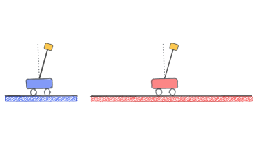
Figure 2: Cartpole: in-distribution setting (blue) and OOD setting (red).

Cartpole [39] is a well-known RL benchmark in which an agent controls the movement of a cart with an upside-down pendulum (“pole”) attached to its top. The cart moves on a platform and the agent’s goal is to keep the pole balanced for as long as possible (see Fig. 2).

Agent and Environment. The agent’s inputs are $s=(x,v_{x},\theta,v_{\theta})$, where $x$ represents the cart’s location on the platform, $\theta$ represents the pole’s angle (i.e., $|\theta|\approx 0$ for a balanced pole, $|\theta|\approx 90\degree$ for an unbalanced pole), $v_{x}$ represents the cart’s horizontal velocity and $v_{\theta}$ represents the pole’s angular velocity.

In-Distribution Inputs. During training, the agent is incentivized to balance the pole, while staying within the platform’s boundaries. In each iteration, the agent’s single output indicates the cart’s acceleration (sign and magnitude) for the next step. During training, we defined the platform’s bounds to be $[-2.4,2.4]$, and the cart’s initial position as near-static, and close to the center of the platform (left-hand side of Fig. 2). This was achieved by drawing the cart’s initial state vector values uniformly from the range $[-0.05,0.05]$.

(OOD) Input Domain. We consider an input domain with larger platforms than the ones used in training. To wit, we now allow the $x$ coordinate of the input vectors to cover a wider range of $[-10,10]$. For the other inputs, we used the same bounds as during the training. See Appendices A and B for additional details.

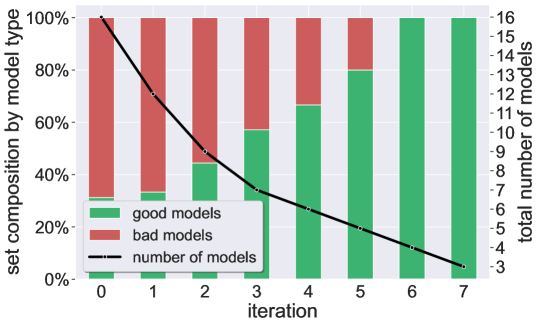
Figure 3: Cartpole: Alg. 2’s results, per iteration: the bars reflect the ratio between the good/bad models (left y-axis) in the surviving set of models, and the curve indicates the number of surviving models (right y-axis).

Evaluation. We trained $k=16$ models, all of which achieved high rewards during training on the short platform. Next, we ran Alg. 2 until convergence ($7$ iterations, in our experiments) on the aforementioned input domain, resulting in a set of $3$ models. We then tested all $16$ original models using (OOD) inputs drawn from the new domain, such that the generated distribution encodes a novel setting: the cart is now placed at the center of a much longer, shifted platform (see the red cart in Fig. 2).

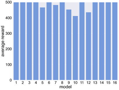
(a)

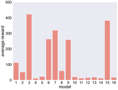
(b)

Figure 9: Cartpole: models’ average rewards in different distributions.

All other parameters in the OOD environment were identical to those used for the original training. Fig. 9 (in the Appendix) depicts the results of evaluating the models using $20,000$ OOD instances. Of the original $16$ models, $11$ scored a low-to-mediocre average reward, indicating their poor ability to generalize to this new distribution. Only $5$ models obtained high reward values, including the $3$ models identified by Alg. 2; thus implying that our method was able to effectively remove all $11$ models that would have otherwise performed poorly in this OOD setting (see Fig. 3). For additional information, see Appendix D.

4.2 Mountain Car

For our second experiment, we evaluated our method on the Mountain Car [86] benchmark, in which an agent controls a car that needs to learn how to escape a valley and reach a target. As in the Cartpole experiment, we selected a set of models that performed well in-distribution and applied our method to identify a subset of models that make similar decisions in a predefined input domain. We again generated OOD inputs (relative to the training) from within this domain, and observed that the models selected by our algorithm indeed generalize significantly better than their peers that were iteratively removed. Detailed information about this benchmark can be found in Appendix E.

4.3 Aurora Congestion Controller

In our third benchmark, we applied our method to a complex, real-world system that implements a policy for Internet congestion control. The goal of congestion control is to determine, for each traffic source in a communication network, the pace at which data packets should be sent into the network. Congestion control is a notoriously difficult and fundamental challenge in computer networking [65, 75]; sending packets too fast might cause network congestion, leading to data loss and delays. Conversely, low sending rates might under-utilize available network bandwidth. Aurora [50] is a DRL-based congestion controller that is the subject of recent work on DRL verification [34, 8]. In each time-step, an Aurora agent observes statistics regarding the network and decides the packet sending rate for the following time-step. For example, if the agent observes excellent network conditions (e.g., no packet loss), we expect it to increase the packet sending rate to better utilize the network. We note that Aurora handles a much harder task than classical RL benchmarks (e.g., Cartpole and Mountain Car): congestion controllers must react gracefully to various possible events based on nuanced signals, as reflected by Aurora’s inputs. Here, unlike in the previous benchmarks, it is not straightforward to characterize the optimal policy.

Agent and Environment. Aurora’s inputs are $t$ vectors $v_{1},\ldots,v_{t}$, representing observations from the $t$ previous time-steps. The agent’s single output value indicates the change in the packet sending rate over the next time-step. Each vector $v_{i}\in\mathbb{R}^{3}$ includes three distinct values, representing statistics that reflect the network’s condition (see details in Appendix F). In line with previous work [34, 50, 8], we set $t=10$ time-steps, making Aurora’s inputs of size $3t=30$. The reward function is a linear combination of the data sender’s throughput, latency, and packet loss, as observed by the agent (see [50] for additional details).

In-Distribution Inputs. Aurora’s training applies the congestion controller to simple network scenarios where a single sender sends traffic towards a single receiver across a single network link. Aurora is trained across varying choices of initial sending rate, link bandwidth, link packet-loss rate, link latency, and size of the link’s packet buffer. During training, packets are initially sent by Aurora at a rate corresponding to $0.3-1.5$ times the link’s bandwidth.

(OOD) Input Domain. In our experiments, the input domain encoded a link with a shallow packet buffer, implying that only a few packets can accumulate in the network (while most excess traffic is discarded), causing the link to exhibit a volatile behavior. This is captured by the initial sending rate being up to $8$ times the link’s bandwidth, to model the possibility of a dramatic decrease in available bandwidth (e.g., due to competition, traffic shifts, etc.). See Appendix F for additional details.

Evaluation. We ran our algorithm and scored the models based on their disagreement upon this large domain, which includes inputs they had not encountered during training, representing the aforementioned novel link conditions.

Experiment (1): High Packet Loss. In this experiment, we trained over $100$ Aurora agents in the original (in-distribution) environment. Out of these, we selected $k=16$ agents that achieved a high average reward in-distribution (see Fig. LABEL:subfig:auroraRewards:inDist). Next, we evaluated these agents on OOD inputs that are included in the previously described domain. The main difference between the training distribution and the new (OOD) ones is the possibility of extreme packet loss rates upon initialization.

Our evaluation over the OOD inputs, within the domain, indicates that although all $16$ models performed well in-distribution, only $7$ agents could successfully handle such OOD inputs (see Fig. LABEL:subfig:auroraRewards:OOD). When we ran Alg. 2 on the 16 models, it was able to filter out all $9$ models that generalized poorly on the OOD inputs (see Fig. 4). In particular, our method returned model $\{16\}$, which is the best-performing model according to our simulations. We note that in the first iterations, the four models to be filtered out were models $\{1,2,6,13\}$, which are indeed the four worst-performing models on the OOD inputs (see Appendix F).

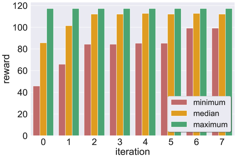
(a) Reward statistics of remaining models

(b) Ratio between good/bad models

Figure 4: Aurora: Alg. 2’s results, per iteration.

Experiment (2): Additional Distributions over OOD Inputs. To further demonstrate that, in the specified input domain, our method is indeed likely to keep better-performing models while removing bad models, we reran the previous Aurora experiments for additional distributions (probability density functions) over the OOD inputs. Our evaluation reveals that all models removed by Alg. 2 achieved low reward values also for these additional distributions (see Appendix F). These results highlight an important advantage of our approach: it applies to all inputs within the considered domain, and so it applies to all distributions over these inputs.

Additional Experiments. We also generated a new set of Aurora models by altering the training process to include significantly longer interactions. We then repeated the aforementioned experiments. The results (summarized in Appendix F) demonstrate that our approach (again) successfully selected a subset of models that generalizes well to distributions over the OOD input domain.

4.4 Comparison to Additional Methods

Gradient-based methods [46, 69, 68, 59] are optimization algorithms capable of finding DNN inputs that satisfy prescribed constraints, similarly to verification methods. These algorithms are extremely popular due to their simplicity and scalability. However, this comes at the cost of being inherently incomplete and not as precise as DNN verification [110, 10]. Indeed, when modifying our algorithm to calculate PDT scores with gradient-based methods, the results (summarized in Appendix G) reveal that, in our context, the verification-based approach is superior to the gradient-based ones. Due to the incompleteness of gradient-based approaches [110], they often computed sub-optimal PDT values, resulting in models that generalize poorly being retained.

Predictive uncertainty methods [80, 1] are online methods for assessing uncertainty with respect to observed inputs, to determine whether an encountered input is drawn from the training distribution. We ran an experiment comparing our approach to uncertainty-prediction-based model selection: we generated ensembles [57, 27, 36] of our original models, and used a variance-based metric (motivated by [64]) to identify subsets of models with low output variance on OOD-sampled inputs. Similar to gradient-based methods, predictive-uncertainty techniques proved fast and scalable, but lacked the precision afforded by verification-driven model selection and were unable to discard poorly generalizing models. For example, when ranking Cartpole models by their uncertainty on OOD inputs, the three models with the lowest uncertainty included also “bad” models, which had been filtered out by our approach.

5 Related Work

Recently, a plethora of approaches and tools have been put forth for ensuring DNN correctness [31, 52, 53, 54, 47, 58, 42, 95, 37, 101, 63, 55, 109, 92, 82, 76, 43, 67, 111, 20, 107, 14, 29, 30, 98, 35, 38, 89, 48, 103, 96, 113, 40, 28, 104, 115, 49, 2], including techniques for DNN shielding [66], optimization [13, 97], quantitative verification [15], abstraction [84, 11, 95, 114, 79, 12], size reduction [83], and more. Non-verification techniques, including runtime-monitoring [45], ensembles [112, 78, 88, 77] and additional methods [81] have been utilized for OOD input detection.

In contrast to the above approaches, we aim to establish generalization guarantees with respect to an entire input domain (spanning all distributions across this domain). In addition, to the best of our knowledge, ours is the first attempt to exploit variability across models for distilling a subset thereof, with improved generalization capabilities. In particular, it is also the first approach to apply formal verification for this purpose.

6 Conclusion

This work describes a novel, verification-driven approach for identifying DNN models that generalize well to an input domain of interest. We presented an iterative scheme that employs a backend DNN verifier, allowing us to score models based on their ability to produce similar outputs on the given domain. We demonstrated extensively that this approach indeed distills models capable of good generalization. As DNN verification technology matures, our approach will become increasingly scalable, and also applicable to a wider variety of DNNs.

Acknowledgements. The work of Amir, Zelazny, and Katz was partially supported by the Israel Science Foundation (grant number 683/18). The work of Amir was supported by a scholarship from the Clore Israel Foundation. The work of Maayan and Schapira was partially supported by funding from Huawei.

Appendices

Appendix A Training and Evaluation

In this appendix, we elaborate on the hyperparameters and the training procedure, for reproducing all models and environments of all three benchmarks. We also provide a thorough overview of various implementation details. The code is based on the Stable-Baselines 3 [85] and OpenAI Gym [19] packages. Unless stated otherwise, the values of the various parameters used during training and evaluation are the default values (per training algorithm, environment, etc.). Our original code and models are publicly available online [7].

A.1 Training Algorithm

We trained our models with Actor-Critic algorithms. These are state-of-the-art RL training algorithms that iteratively optimize two neural networks:

• a critic network, that learns a value function [73] (also known as a Q-function), that assigns a value to each $\langle$state,action$\rangle$ pair; and

• an actor network, which is the DRL-based agent trained by the algorithm. This network iteratively maximizes the value function learned by the critic, thus improving the learned policy.

Specifically, we used two implementations of Actor-Critic algorithms: Proximal Policy Optimization (PPO) [91] and Soft Actor-Critic (SAC) [44].

Actor-Critic algorithms are considered very advantageous, due to their typical requirement of relatively few samples to learn from, and also due to their ability to allow the agent to learn policies for continuous spaces of $\langle$state,action$\rangle$ pairs.

In each training process, all models were trained using the same hyperparameters, with the exception of the Pseudo Random Number Generator’s (PRNG) seed. Each training phase consisted of $10$ checkpoints, while each checkpoint included a constant number of environment steps, as described below. For model evaluation, we used the last checkpoint of each training process (per benchmark).

A.2 Architecture

In all benchmarks, we used DNNs with a feed-forward architecture. We refer the reader to Table 1 for a summary of the chosen architecture per each benchmark.

benchmark	hidden layers	layer size	activation function	training algorithm
Cartpole	2	[32, 16]	ReLU	PPO
Mountain Car	2	[64, 16]	ReLU	SAC
Aurora	2	[32, 16]	ReLU	PPO

Table 1: DNN architectures and training algorithms, per benchmark.

A.3 Cartpole Parameters

A.3.1 Architecture and Training

1. Architecture

   • hidden layers: 2

   • size of hidden layers: 32 and 16, respectively

   • activation function: ReLU

2. Training

   • algorithm: Proximal Policy Optimization (PPO)

   • gamma ($\gamma$): 0.95

   • batch size: 128

   • number of checkpoints: $10$

   • total time-steps (number of training steps for each checkpoint): $50,000$

   • PRNG seeds (each one used to train a different model):
     $\{1,2,3,4,5,6,7,8,9,10,11,12,13,14,15,16\}$

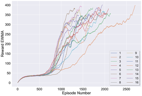
Figure 5: Cartpole: models’ reward exponential weighted moving average (EWMA). All models achieved a high reward (at the end of their training).

A.3.2 Environment

We used the configurable CartPoleContinuous-v0 environment. Given lower and upper bounds for the x-axis location, denoted as $[low,high]$, and $mid=\frac{high+low}{2}$, the initial x position is randomly, uniformly drawn from the interval $[mid-0.05,mid+0.05]$.

An episode is a sequence of agent interactions with the environment, which ends when a terminal state is reached. In the Cartpole environment, an episode terminates after the first of the following occurs:

1. The cart’s location exceeds the platform’s boundaries (as expressed via the $x$-axis location); or

2. The cart was unable to balance the pole, which fell (as expressed via the $\theta$-value); or

3. $500$ time-steps have passed

A.3.3 Domains

1. (Training) In-Distribution

   • action min magnitude: True

   • x-axis lower bound (x_threshold_low): $-2.4$

   • x-axis upper bound (x_threshold_high): $2.4$

2. (OOD) Input Domain

   Two symmetric OOD scenarios were evaluated: the cart’s $x$ position represented significantly extended platforms in a single direction, hence, including areas previously unseen during training. Specifically, we generated a domain of input points characterized by $x$-axis boundaries that were selected, with an equal probability, either from $[-10,-2.4]$ or from $[2.4,10]$ (instead of the in-distribution range of $[-2.4,2.4])$. The cart’s initial location was uniformly drawn from the range’s center $\pm 0.05$: $[-6.4-0.05,-6.4+0.05]$ and $[6.4-0.05,6.4+0.05]$, respectively.

   All other parameters were the same as the ones used in-distribution.

   OOD scenario 1

   • x-axis lower bound (x_threshold_low): $-10.0$

   • x-axis upper bound (x_threshold_high): $-2.4$

   OOD scenario 2

   • x-axis lower bound (x_threshold_low): $2.4$

   • x-axis upper bound (x_threshold_high): $10.0$

A.4 Mountain Car Parameters

A.4.1 Architecture and Training

1. Architecture

   • hidden layers: 2

   • size of hidden layers: 64 and 16, respectively

   • activation function: ReLU

   • clip mean parameter: 5.0

   • log stdinit parameter: -3.6

2. Training

   • algorithm: Soft Actor Critic (SAC)

   • gamma ($\gamma$): 0.9999

   • batch size: 512

   • buffer size: 50,000

   • gradient steps: 32

   • learning rate: $3\text{\times}{10}^{-4}$

   • learning starts: 0

   • tau ($\tau$): 0.01

   • train freq: 32

   • use sde: True

   • number of checkpoints: $10$

   • total time-steps (number of training steps for each checkpoint): $5,000$

   • PRNG seeds (each one used to train a different model):
     $\{1,2,3,4,5,6,7,8,9,10,11,12,13,14,15,16\}$

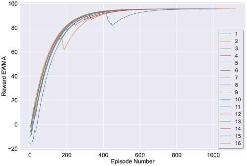
Figure 6: Mountain Car: models’ reward exponential weighted moving average (EWMA). All models achieved a high reward (at the end of their training).

A.4.2 Environment

We used the MountainCarContinuous-v1 environment.

A.4.3 Domains

1. (Training) In-Distribution

   • min position: $-1.2$

   • max position: $-0.6$

   • goal position: $0.45$

   • min action (if the agent’s action is negative and under this value, this value is used): $-2$

   • max action (if the agent’s action is positive and above this value, this value is used): $2$

   • max speed: $0.4$

   • initial location range (from which the initial location is uniformly drawn): $[-0.9,-0.6]$

   • initial velocity range (from which the initial velocity is uniformly drawn): $[0,0]$ (i.e., the initial velocity in this scenario is always $0$)

   • x scale factor (used for scaling the x-axis): $1.5$

2. (OOD) Input Domain

   The inputs are the same as the ones used in-distribution, except for the following:

   • min position: $-2.4$

   • max position: $1.2$

   • goal position: $0.9$

   • initial location range: $[0.4,0.5]$

   • initial location velocity: $[-0.4,-0.3]$

A.5 Aurora Parameters

A.5.1 Architecture and Training

1. Architecture

   • hidden layers: 2

   • size of hidden layers: 32 and 16, respectively

   • activation function: ReLU

2. Training

   • algorithm: Proximal Policy Optimization (PPO)

   • gamma ($\gamma$): 0.99

   • number of steps to run for each environment, per update (n_steps): $8,192$

   • Number of epochs when optimizing the surrogate loss (n_epochs): $4$

   • learning rate: $1\text{\times}{10}^{-3}$

   • Value function loss coefficient (vf_coef): $1$

   • Entropy function loss coefficient (ent_coef): $1\text{\times}{10}^{-2}$

   • number of checkpoints: $6$

   • total time-steps (number of training steps for each checkpoint): $656,000$ (as used in the original paper [50])

   • PRNG seeds (each one used to train a different model):
     $\{4,52,105,666,850,854,857,858,885,897,901,906,907,929,944,945\}$
     We note that for simplicity, these were mapped to indices $\{1\ldots 16\}$, accordingly (e.g., $\{4\}\rightarrow\{1\}$, $\{52\}\rightarrow\{2\}$, etc.).

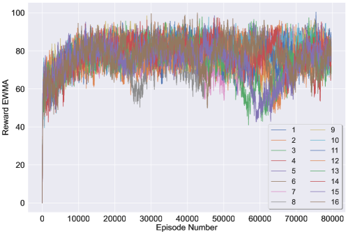
Figure 7: Aurora (short training): models’ reward exponential weighted moving average (EWMA) during training. All models achieved a high reward (at the end of their training).

A.5.2 Environment

We used a configurable version of the PccNs-v0 environment. For models in Exp. 4.3(with the short training), each episode consisted of $50$ steps. For models in Exp. 20 (with the long training), each episode consisted of $400$ steps.

A.5.3 Domains

1. (Training) In-Distribution

   • minimal initial Sending Rate ratio (to the link’s bandwidth) (min_initial_send_rate_bw_ratio): $0.3$

   • maximal initial Sending Rate ratio (to the link’s bandwidth) (max_initial_send_rate_bw_ratio): $1.5$

2. (OOD) Input Domain

   To bound the latency gradient and latency ratio elements of the input, we used a shallow buffer setup, with a bounding parameter $\delta>0$ such that latency gradient $\in[-\delta,\delta]$ and latency ratio $\in[1.0,1.0+\delta]$.

   • minimal initial sending rate ratio (to the link’s bandwidth) (min_initial_send_rate_bw_ratio): $2.0$

   • maximal initial sending rate ratio (to the link’s bandwidth) (max_initial_send_rate_bw_ratio): $8.0$

   • Use shallow buffer: True

   • Shallow buffer $\delta$ bound parameter: $1\text{\times}{10}^{-2}$

Appendix B Verification Queries

B.1 A DNN Verification Query: Toy Example

Let us revisit the DNN in Fig. 1. Suppose that we wish to verify that for all nonnegative inputs the DNN outputs a value strictly smaller than $25$, i.e., for all inputs $x=\langle v_{1}^{1},v_{1}^{2}\rangle\in\mathbb{R}^{2}_{\geq 0}$, it holds that $N(x)=v_{4}^{1}<25$. This is encoded as a verification query by choosing a precondition restricting the inputs to be non-negative, i.e., $P=(v^{1}_{1}\geq 0\wedge v_{1}^{2}\geq 0)$, and by setting $Q=(v_{4}^{1}\geq 25)$, which is the negation of our desired property. For this specific verification query, a sound verifier will return SAT, alongside a feasible counterexample such as $x=\langle 0,4\rangle$, which produces $v_{4}^{1}=28\geq 25$. Hence, this property does not hold for the DNN described in Fig. 1. All queries were dispatched to Marabou [54] — a sound and complete verification engine, previously used in other DNN-verification-related work [10, 9, 5, 21, 49, 110, 108, 95, 33, 79, 26, 17, 32, 6, 23].

B.2 Input Domain Queries

Next, we elaborate on how we encoded the queries, which we later fed to our backend verification engine, in order to compute the PDT scores for a DNN pair. Given a DNN pair, $N_{1}$ and $N_{2}$, we execute the following stages:

1. We concatenate $N_{1}$ and $N_{2}$ to a new DNN $N_{3}=[N_{1};N_{2}]$, which is roughly twice the size of each of the original DNNs (as both $N_{1}$ and $N_{2}$ have the same architecture). The input of $N_{3}$ is of the same original size as each single DNN and is connected to the second layer of each DNN, consequently allowing the same input to flow throughout the network to the output layer of each original DNN ($N_{1},N_{2}$). Thus, the output layer of $N_{3}$ is a concatenation of the outputs of both $N_{1}$ and $N_{2}$. A scheme depicting the construction of a concatenated DNN appears in Fig. 8.

   

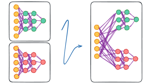
   Figure 8: In order to calculate the PDT scores, we generated a new DNN which is the concatenation of each pair of DNNs, sharing the same input.

2. Encoding a precondition P which represents the ranges of the input variables. We used these inputs to include values in the input domains of interest. In some cases, these values were predefined to match the OOD setting evaluated, and in others, we extracted these values based on empirical simulations of the models post-training. As we mentioned before, the bounds are supplied by the system designer, based on prior knowledge of the input domain. In our experiments, we used the following bounds of the input domain:

   1. Cartpole:

      • x position: $x\in[-10,-2.4]$ or $x\in[2.4,10]$ The PDT was set to be the maximum PDT score of each of these two scenarios.

      • $x$ velocity: $v_{x}\in[-2.18,2.66]$

      • angle: $\theta\in[-0.23,0.23]$

      • angular velocity: $v_{\theta}\in[-1.3,1.22]$

   2. Mountain Car:

      • x position: $x\in[-2.4,0.9]$

      • $x$ velocity: $v_{x}\in[-0.4,0.134]$

   3. Aurora:

      • latency gradient: $x_{t}\in[-0.007,0.007]$, for all $t$ s.t. $(t\mod 3)=0$

      • latency ratio: $x_{t}\in[1,1.04]$, for all $t$ s.t. $(t\mod 3)=1$

      • sending ratio: $x_{t}\in[0.7,8]$, for all $t$ s.t. $(t\mod 3)=2$

3. Encoding a postcondition Q which encodes (for a fixed slack $\alpha$) and a given distance function $d:\mathcal{O}\times\mathcal{O}\mapsto\mathbb{R^{+}}$, that for an input $x^{\prime}\in\Psi$ the following holds: $d(N_{1}(x^{\prime}),N_{2}(x^{\prime}))\geq\alpha$

   Examples of distance functions:

   1. $L_{1}$ norm:

      $$d(N_{1},N_{2})=\operatorname*{arg\,max}_{x\in\Psi}(|N_{1}(x)-N_{2}(x)|)$$

      This distance function was used in the case of the Aurora benchmark.

   2. $\mathbf{condition-distance(``c-distance^{\prime\prime})}$: the $c-distance$ function returns the maximal $L_{1}$ norm of two DNNs, for all inputs $x\in\Psi$ such that both outputs $N_{1}(x)$, $N_{2}(x)$ comply to constraint $\mathbf{c}$.

      $$c-distance(N_{1},N_{2})\triangleq\max_{x\in\Psi\text{ s.t. }N_{1}(x),N_{2}(x)\vDash c}(|N_{1}(x)-N_{2}(x)|)$$

      For the Cartpole and Mountain Car benchmarks, we defined the distance function to be:

      $$d(N_{1},N_{2})=\min_{c,c^{\prime}}(c-distance(N_{1},N_{2}),c^{\prime}-distance(N_{1},N_{2}))$$

      We chose $c:=N_{1}(x)\geq 0\wedge N_{2}(x)\geq 0$ and $c^{\prime}:=N_{1}(x)\leq 0\wedge N_{2}(x)\leq 0$

      This distance function is tailored to find the maximal difference between the outputs (actions) of two models, in a given category of inputs (non-positive or non-negative, in our case). The intuition behind this function is that in some benchmarks, good and bad models may differ in the sign (rather than only the magnitude) of their actions. For example, consider a scenario of the Cartpole benchmark where the cart is located on the “edge” of the platform: an action to one direction (off the platform) will cause the episode to end, while an action to the other direction will allow the agent to increase its rewards by continuing the episode.

Appendix C Algorithm Variations and Hyperparameters

In this appendix, we elaborate on our algorithms’ additional hyperparameters and filtering criteria, used throughout our evaluation. As the results demonstrate, our method is highly robust in a myriad of settings.

C.1 Precision

For each benchmark and each experiment, we arbitrarily selected $k=16$ models which reached our reward threshold for the in-distribution data. Then, we used these models for our empirical evaluation. The PDT scores were calculated up to a finite precision of $0.5\leq\epsilon\leq 1$, depending on the benchmark ($1$ for Cartpole and Aurora, and $0.5$ for Mountain Car).

C.2 Filtering Criteria

As elaborated in Section 3, our algorithm iteratively filters out (Line 8 in Alg. 2) models with a relatively high disagreement score, i.e., models that may disagree with their peers in the inputs domain. We present three different criteria in which we may choose the models to remove in a given iteration, after sorting the models based on their DS score:

1. PERCENTILE: in which we remove the top $p\%$ of models with the highest disagreement scores, for a predefined value $p$. In our experiments, we chose $p=25\%$.

2. MAX: in which we:

   1. sort the DS scores of all models in a descending order

   2. calculate the difference between every two adjacent scores

   3. search for the greatest difference of any two subsequent DS scores

   4. for this difference, use the larger DS as a threshold

   5. remove all models with a DS that is greater than or equal to this threshold

3. COMBINED: in which we remove models based either on MAX or PERCENTILE, depending on which criterion eliminates more models in a specific iteration.

Appendix D Cartpole: Supplementary Results

Throughout our evaluations of this benchmark, we use a threshold of 250 to distinguish between good and bad models — this threshold value induces a large margin from rewards of poorly-performing models (which are usually less than $100$).

Note that as seen in Fig. 10, our algorithm eventually also removes some of the more successful models. However, the final result contains only well-performing models, as in the other benchmarks.

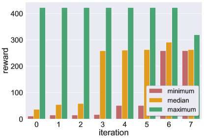
Figure 10: Cartpole: model selection results: minimum, median, and maximum rewards of the models selected after each iteration.

D.1 Result per Filtering Criteria

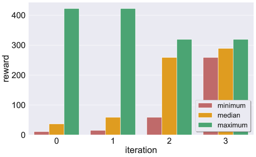
(a) Rewards statistics

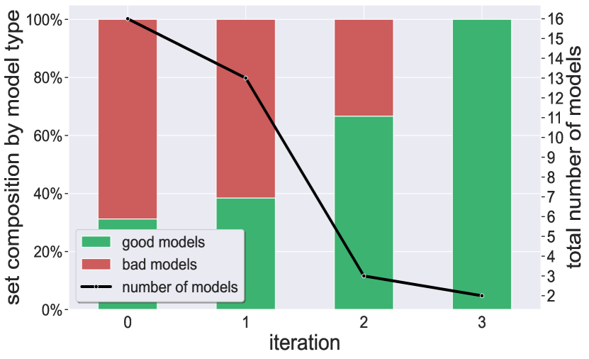
(b) Remaining good and bad models ratio

Figure 11: Cartpole: results using the MAX filtering criterion.

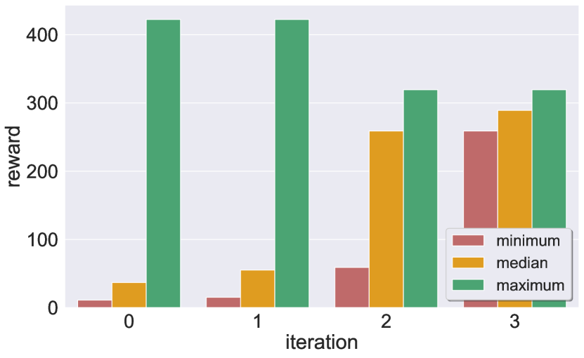
(a) Rewards statistics

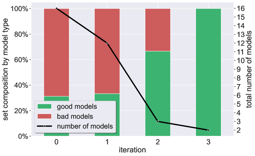
(b) Remaining good and bad models ratio

Figure 12: Cartpole: results using the COMBINED filtering criterion.

Appendix E Mountain Car: Supplementary Results

E.1 The Mountain Car Benchmark

Mountain Car is a classic, relatively simple RL benchmark. In this benchmark, a car (agent) is placed in a valley between two hills (at $x\in[-1.2,0.6]$), and needs to reach a flag on top of one of the hills. The state, $s=(x,v_{x})$ represents the car’s location (along the x-axis) and velocity. The agent’s action (output) is the applied force: a continuous value indicating the magnitude and direction in which the agent wishes to move. During training, the agent is incentivized to reach the flag (placed at the top of a valley, originally at $x=0.45$). For each time-step until the flag is reached, the agent receives a small, negative reward; if it reaches the flag, the agent is rewarded with a large positive reward. An episode terminates when the flag is reached, or when the number of steps exceeds some predefined value ($300$ in our experiments). Good and bad models are distinguished by an average reward threshold of 90.

During training (in-distribution), the car is initially placed on the left side of the valley’s bottom, with a low, random velocity (see Fig. 13(a)). We trained $k=16$ agents (denoted as $\{1,2,\ldots 16\}$), which all perform well (i.e., achieve an average reward higher than our threshold) in-distribution. This evaluation was done for over $10,000$ episodes.

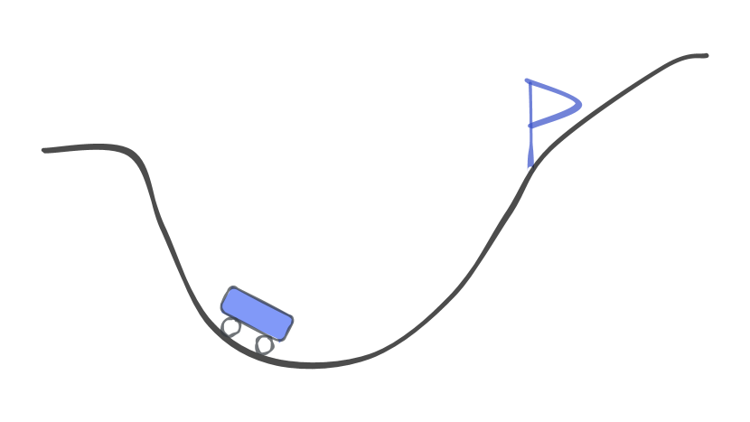
(a) Training (in-distribution) setting: the agent’s initial point is on the left side, and the goal is at a nearby point

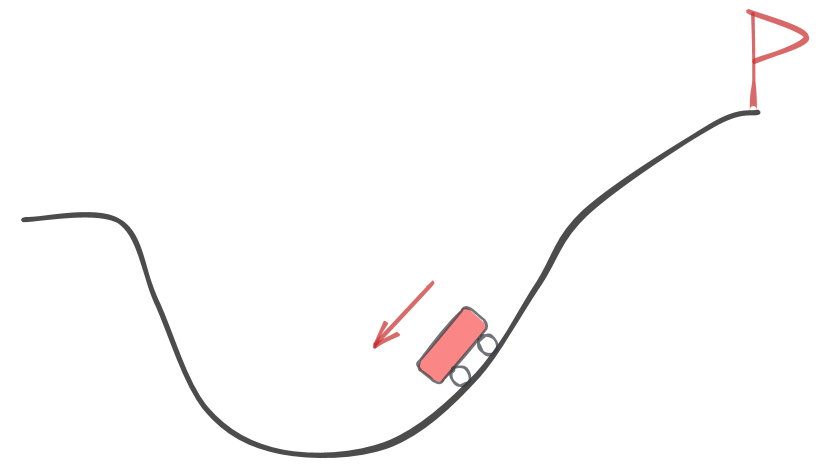
(b) OOD setting: the agent’s initial point is farther away, with initial negative velocity; the goal is significantly farther up than in training

Figure 13: Mountain Car: figure (a) depicts the setting on which the agents were trained, and figure (b) depicts the harder, OOD setting.

According to the scenarios used by the training environment, we specified the (OOD) input domain by: (i) extending the x-axis, from $[-1.2,0.6]$ to $[-2.4,0.9]$; (ii) moving the flag further to the right, from $x=0.45$ to $x=0.9$; and (iii) setting the car’s initial location further to the right of the valley’s bottom, and with a large initial negative velocity (to the left). An illustration appears in Fig. 13(b). These new settings represent a novel state distribution, which causes the agents to respond to states that they had not observed during training: different locations, greater velocity, and different combinations of location and velocity directions.

Out of the $k=16$ models that performed well in-distribution, $4$ models failed (i.e., did not reach the flag, ending their episodes with a negative average reward) in the OOD scenario, while the remaining $12$ succeeded, i.e., reached a high average reward when simulated on the OOD data (see Fig. 14). The large ratio of successful models is not surprising, as Mountain Car is a relatively easy benchmark.

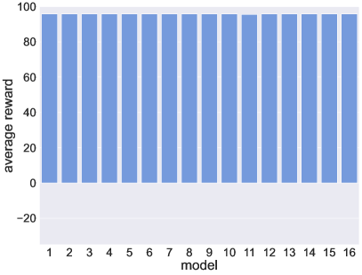
(a)

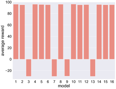
(b)

Figure 14: Mountain Car: the models’ average rewards in different distributions.

To evaluate our algorithm, we ran it on these models, and the aforementioned (OOD) input domain, and checked whether it removed the models that (although successful in-distribution) fail in the new, harder, setting. Indeed, our method was able to filter out all unsuccessful models, leaving only a subset of $5$ models ($\{2,4,8,10,15\}$), all of which perform well in the OOD scenario.

We also note that our algorithm is robust to various hyperparameters, as demonstrated in Fig. 15, Fig. 16 and Fig. 17 which depict the results of each iteration of our algorithm, when applied with various filtering criteria (elaborated in Appendix C).

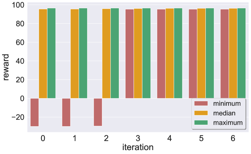
(a) Rewards statistics

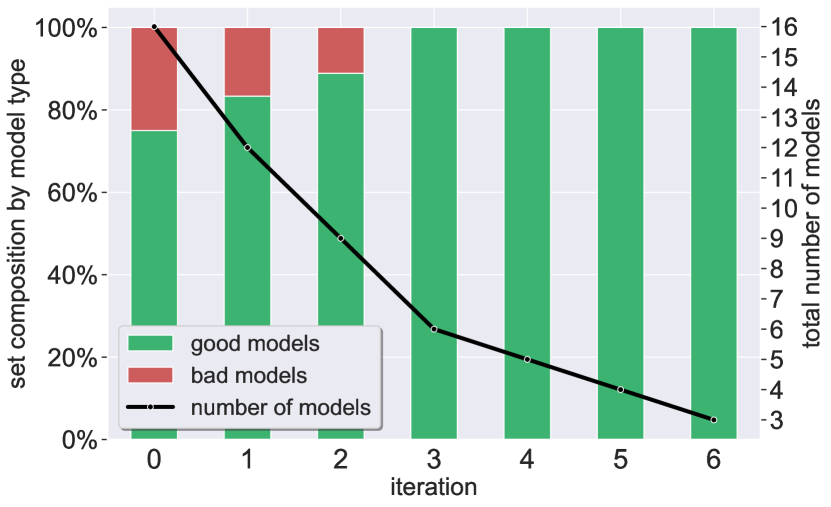
(b) Remaining good and bad models ratio

Figure 15: Mountain Car: results using the PERCENTILE filtering criterion.

E.2 Additional Filtering Criteria

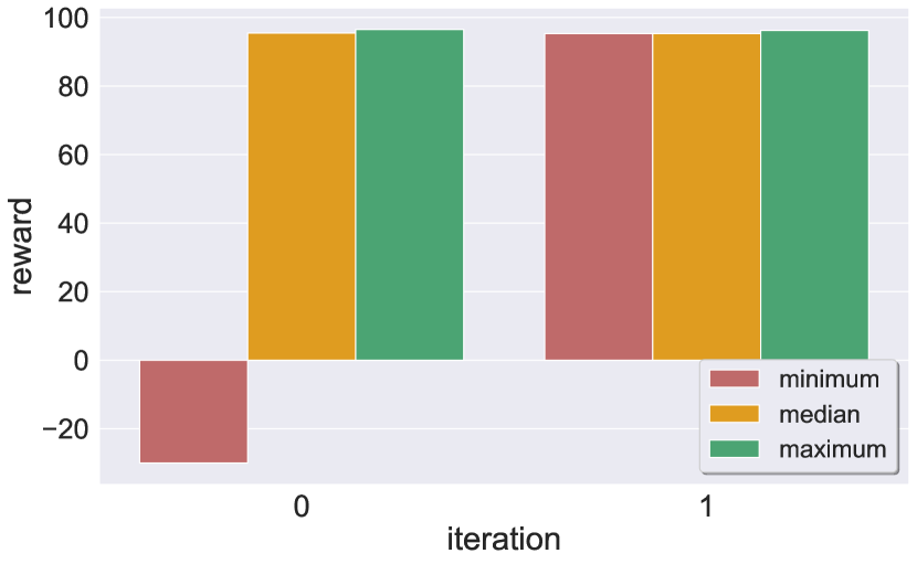
(a) Rewards statistics

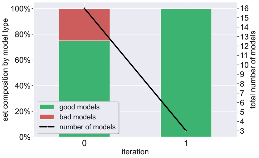
(b) Remaining good and bad models ratio

Figure 16: Mountain Car: results using the MAX filtering criterion.

(a) Rewards statistics

(b) Remaining good and bad models ratio

Figure 17: Mountain Car: results using the COMBINED filtering criterion.

E.3 Combinatorial Experiments

Due to the original bias of the initial set of candidates, in which $12$ out of the original $16$ models are good in the OOD setting, we set out to validate that the fact that our algorithm succeeded in returning solely good models is indeed due to its correctness, and not due to the inner bias among the set of models, to contain good models. In our experiments (summarized below) we artificially generated new sets of models in which the ratio of good models is deliberately lower than in the original set. We then reran our algorithm on all possible combinations of the initial subsets, and calculated (for each subset) the probability to select a good model in this new setting, from the models surviving our filtering process. As we show, our method significantly improves the chances of selecting a good model even when these are a minority in the original set. For example, the leftmost column of Fig. 18 shows that over sets consisting of $4$ bad models and only $2$ good ones, the probability of selecting a good model after running our algorithm is over $60\%$ (!) — almost double the probability of randomly selecting a good model from the original set before running our algorithm. These results were consistent across multiple subset sizes, and with various filtering criteria. We note that for the calculations demonstrating the chance to select a good model, we assume random selection from a subset of models: before applying our algorithm, the subset is the original set of models; and after our algorithm is applied — the subset is updated based on the result of our filtering procedure. The probability is computed based on the number of combinations of bad models surviving the filtering process, and their ratio relative to all the models returned in those cases (we assume uniform probability, per subset).

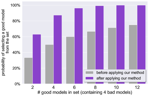
Figure 18: Mountain Car: our algorithm effectively increases the probability to choose a good model, due to effective filtering. The plot corresponds to Table 3.

COMPOSITION		total $\#$ experiments	$\#$ experiments with		probability to choose good models
good	bad	subgroup combinations of good models	all surviving models good	some surviving models bad	naive	our method
12	4	${12\choose{\color[rgb]{0,0.4296875,0.19921875}12}}=1$	1	0	75 %	100%
10	4	${12\choose{\color[rgb]{0,0.4296875,0.19921875}10}}=66$	65	1	71.43 %	99.49 %
8	4	${12\choose{\color[rgb]{0,0.4296875,0.19921875}8}}=495$	423	72	66.67 %	95.15 %
6	4	${12\choose{\color[rgb]{0,0.4296875,0.19921875}6}}=924$	549	375	60 %	86.26 %
4	4	${12\choose{\color[rgb]{0,0.4296875,0.19921875}4}}=495$	123	372	50 %	74.01 %
2	4	${12\choose{\color[rgb]{0,0.4296875,0.19921875}2}}=66$	66	0	33.33 %	54.04 %

Table 2: Results summary of the combinatorial Mountain Car experiment, using the PERCENTILE filtering criterion.

COMPOSITION		total $\#$ experiments	$\#$ experiments with		probability to choose good models
good	bad	subgroup combinations of good models	all surviving models good	some surviving models bad	naive	our method
12	4	${12\choose{\color[rgb]{0,0.4296875,0.19921875}12}}=1$	1	0	75 %	100%
10	4	${12\choose{\color[rgb]{0,0.4296875,0.19921875}10}}=66$	66	0	71.43 %	100 %
8	4	${12\choose{\color[rgb]{0,0.4296875,0.19921875}8}}=495$	486	9	66.67 %	99.34 %
6	4	${12\choose{\color[rgb]{0,0.4296875,0.19921875}6}}=924$	844	80	60 %	96.33 %
4	4	${12\choose{\color[rgb]{0,0.4296875,0.19921875}4}}=495$	375	120	50 %	87.32 %
2	4	${12\choose{\color[rgb]{0,0.4296875,0.19921875}2}}=66$	31	35	33.33 %	63.03 %

Table 3: Results summary of the combinatorial Mountain Car experiment, using the MAX filtering criterion.

COMPOSITION		total $\#$ experiments	$\#$ experiments with		probability to choose good models
good	bad	subgroup combinations of good models	all surviving models good	some surviving models bad	naive	our method
12	4	${12\choose{\color[rgb]{0,0.4296875,0.19921875}12}}=1$	1	0	75 %	100%
10	4	${12\choose{\color[rgb]{0,0.4296875,0.19921875}10}}=66$	66	0	71.43 %	100 %
8	4	${12\choose{\color[rgb]{0,0.4296875,0.19921875}8}}=495$	481	12	66.67 %	99.26 %
6	4	${12\choose{\color[rgb]{0,0.4296875,0.19921875}6}}=924$	842	82	60 %	96.74 %
4	4	${12\choose{\color[rgb]{0,0.4296875,0.19921875}4}}=495$	372	123	50 %	88.09 %
2	4	${12\choose{\color[rgb]{0,0.4296875,0.19921875}2}}=66$	31	35	33.33 %	63.36 %

Table 4: Results summary of the combinatorial Mountain Car experiment, using the COMBINED filtering criterion.

Appendix F Aurora: Supplementary Results

F.1 Additional Information

1. A more detailed explanation of Aurora’s input statistics: (i) Latency Gradient: a derivative of latency (packet delays) over the recent MI (“monitor interval”); (ii) Latency Ratio: the ratio between the average latency in the current MI to the minimum latency previously observed; and (iii) Sending Ratio: the ratio between the number of packets sent to the number of acknowledged packets over the recent MI. As mentioned, these metrics indicate the link’s congestion level.

2. For all our experiments on this benchmark, we defined “good” models as models that achieved an average reward greater than a threshold of 99; “bad” models are models that achieved a reward lower than this threshold.

3. In-distribution, the average reward is not necessarily correlated with the average reward OOD. For example, in Exp. 4.3 with the short episodes during training (see Fig. 20):

   1. In-distribution, model $\{4\}$ achieved a lower reward than models $\{2\}$ and $\{5\}$, but a higher reward OOD.

   2. In-distribution, model $\{16\}$ achieved a lower reward than model $\{15\}$, but a higher reward OOD.

(a) In-distribution setting, in which the agent was trained, with low packet congestion

(b) OOD settings, of a much higher congestion rate, with a significantly greater packet loss

Figure 19: Aurora: illustration of in-distribution and OOD settings.

Experiment(4.3): Aurora: Short Training Episodes

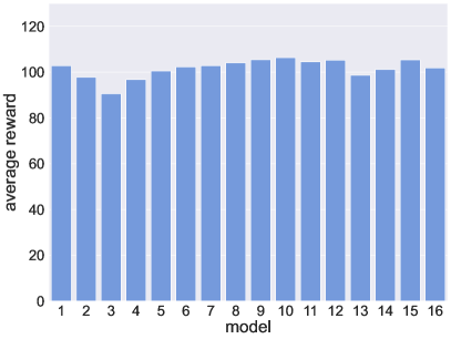
(a)

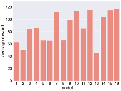
(b)

Figure 20: Aurora Experiment 4.3: the models’ average rewards when simulated on different distributions.

Experiment (3): Aurora: Long Training Episodes

Similar to Experiment 4.3, we trained a new set of $k=16$ agents. In this experiment, we increased each training episode to consist of $400$ steps (instead of $50$, as in the “short” training). The rest of the parameters were identical to the previous setup in Experiment 4.3. This time, $5$ models performed poorly in the OOD environment (i.e., did not reach our reward threshold of $99$), while the remaining $11$ models performed well both in-distribution and OOD.

When running our method with the MAX criterion, our algorithm returned $4$ models, all being a subset of the group of $11$ models which generalized successfully, and after fully filtering out all the unsuccessful models. Running the algorithm with the PERCENTILE or the COMBINED criteria also yielded a subset of this group, indicating the filtering process was again successful (and robust to various algorithm hyperparameters).

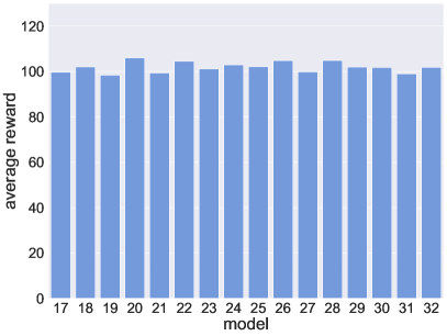
(a)

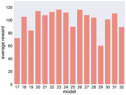
(b)

Figure 21: Aurora Experiment 20: the models’ average rewards when simulated on different distributions.

(a) Rewards statistics

(b) Remaining good and bad models ratio

Figure 22: Aurora Experiment 20: model selection results.

F.2 Additional Probability Density Functions

Following are the results discussed in subsection 4.3, and to further demonstrate our method’s robustness to different types of out-of-distribution inputs, we applied it not only to different values (e.g., high Sending Rate values) but also to various Probability Density Functions (PDFs) of values in the (OOD) input domain in question. More specifically, we repeated the OOD experiments (Experiment 4.3 and Experiment 20) with different PDFs. In their original settings, all of the environment’s parameters (link’s bandwidth, latency, etc.) are uniformly drawn from a range $[low,high]$. However, in this experiment, we generated two additional PDFs: Truncated normal (denoted as $\mathcal{TN}_{[low,high]}(\mu,\sigma^{2})$) distributions that are truncated within the range $[low,high]$). The first PDF was used with $\mu_{low}=0.3*high+(1-0.3)*low$, and the other with a $\mu_{high}=0.8*high+(1-0.8)*low$. For both PDFs, the variance, $\sigma^{2}$, was arbitrarily set to $\frac{high-low}{4}$. These new distributions are depicted in Fig. 23 and were used to test the models from both batches of Aurora experiments (experiments 4.3 and 20).

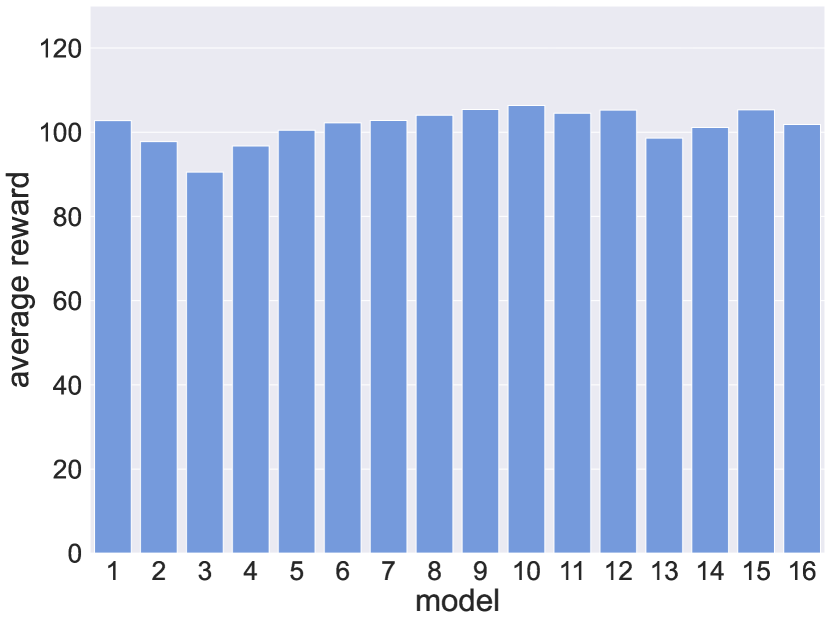
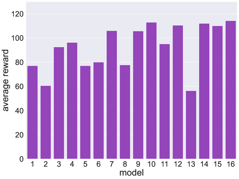
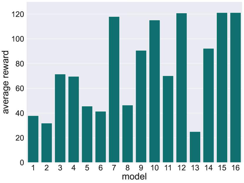
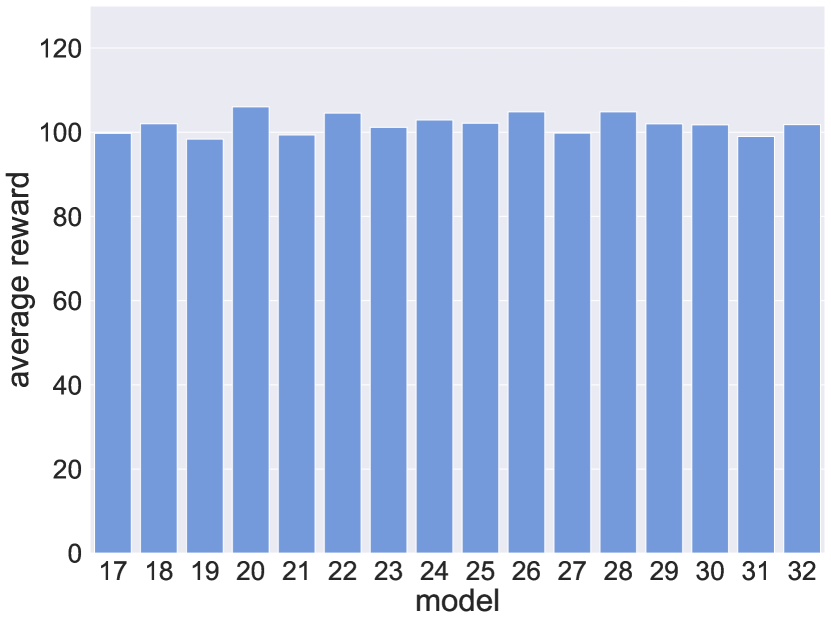
(a) In-distribution
($\sim\mathcal{U}(low,high)$)

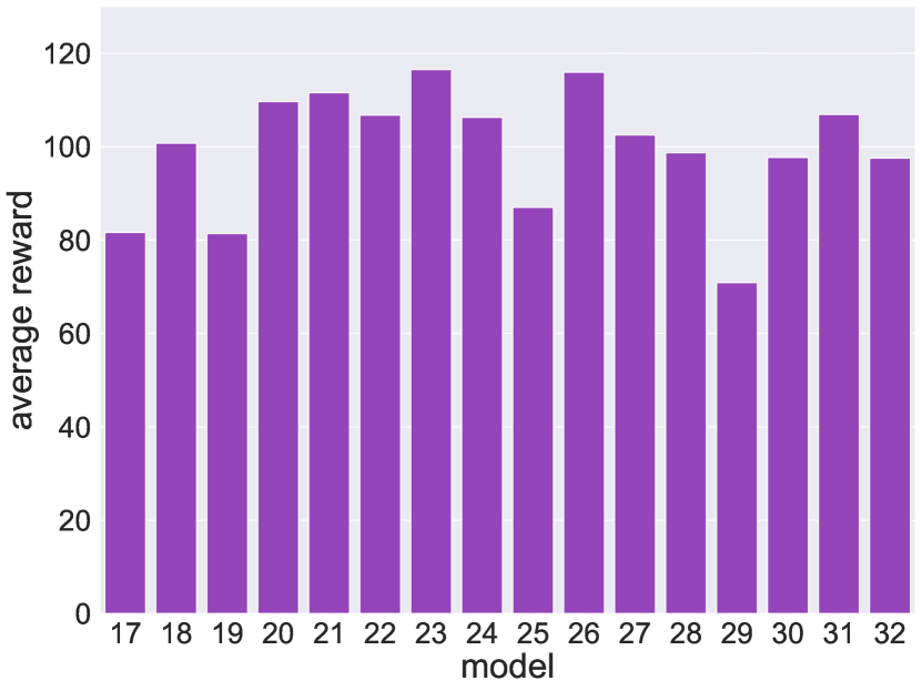
(b) OOD ($\sim\mathcal{TN}(\mu_{low},\sigma^{2}$))

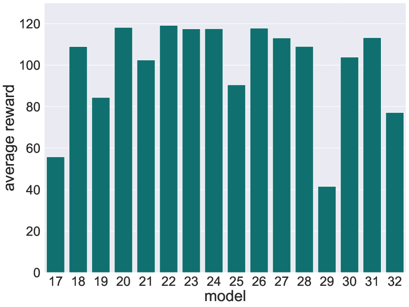
(c) OOD ($\sim\mathcal{TN}(\mu_{high},\sigma^{2}$))

Figure 23: Aurora: the models’ average rewards under different PDFs.
Top row: results for the models used in Experiment 4.3.
Bottom row: results for the models used in Experiment 20.

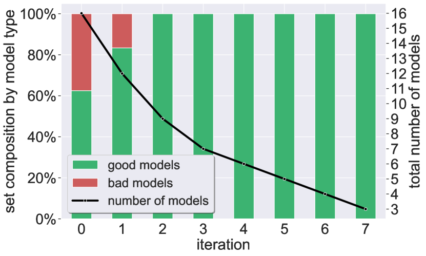
(a) OOD $\sim\mathcal{TN}(\mu_{low},\sigma^{2}$)

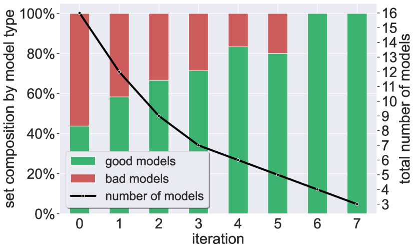
(b) OOD $\sim\mathcal{TN}(\mu_{high},\sigma^{2}$)

Figure 24: Aurora: Additional PDFs: model selection results for OOD values; the models are the same as in Experiment 4.3.

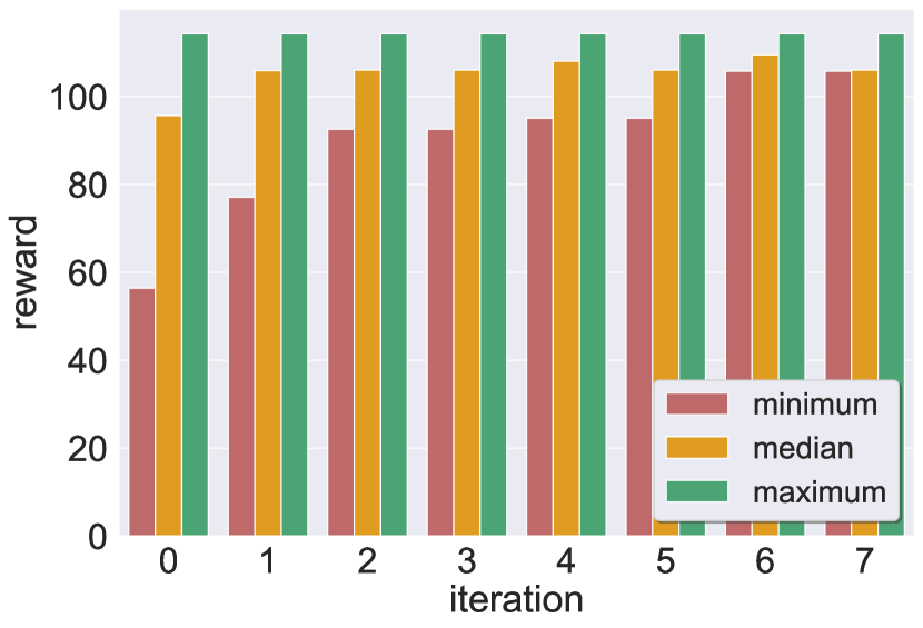
(a) OOD $\sim\mathcal{TN}(\mu_{low},\sigma^{2}$)

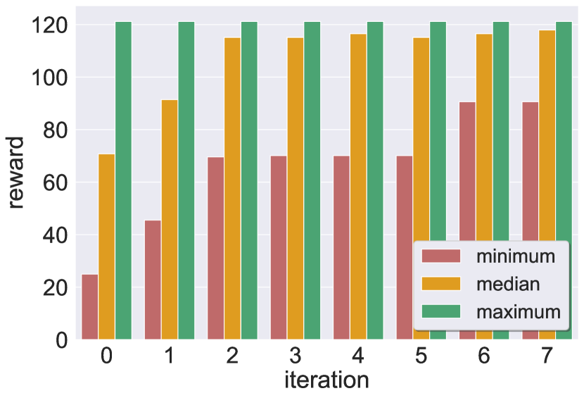
(b) OOD $\sim\mathcal{TN}(\mu_{high},\sigma^{2}$)

Figure 25: Aurora: Additional PDFs: model selection results: rewards statistics per iteration; the models are the same as in Experiment 4.3.

(a) $\sim\mathcal{TN}(\mu_{low},\sigma^{2}$)

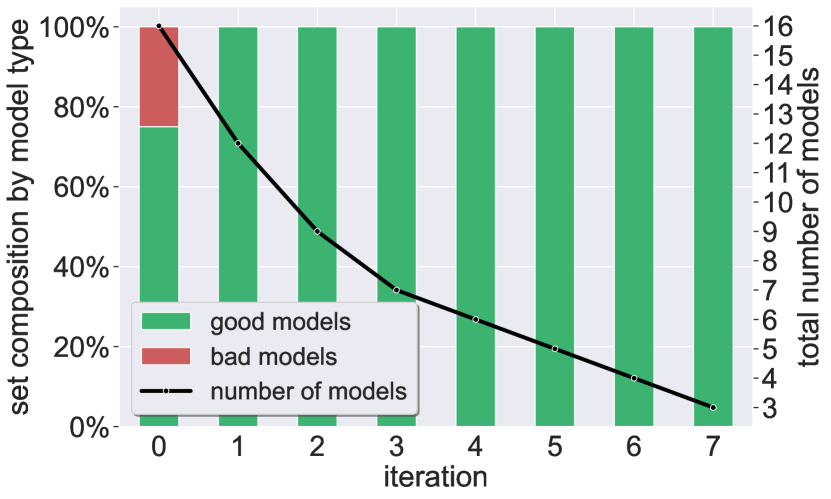
(b) $\sim\mathcal{TN}(\mu_{high},\sigma^{2}$)

Figure 26: Aurora: Additional PDFs: model selection results for OOD values; the models are the same as in Experiment 20.

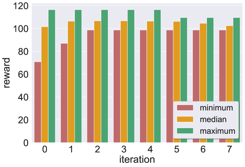
(a) $\sim\mathcal{TN}(\mu_{low},\sigma^{2}$)

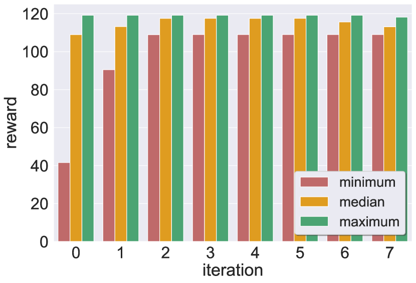
(b) $\sim\mathcal{TN}(\mu_{high},\sigma^{2}$)

Figure 27: Aurora: Additional PDFs: model selection results: rewards statistics per iteration; the models are the same as in Experiment 20.

F.3 Additional Filtering Criteria: Experiment 4.3

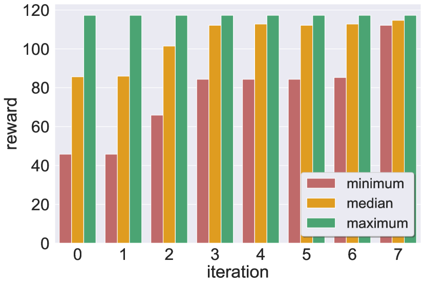
(a) Rewards statistics

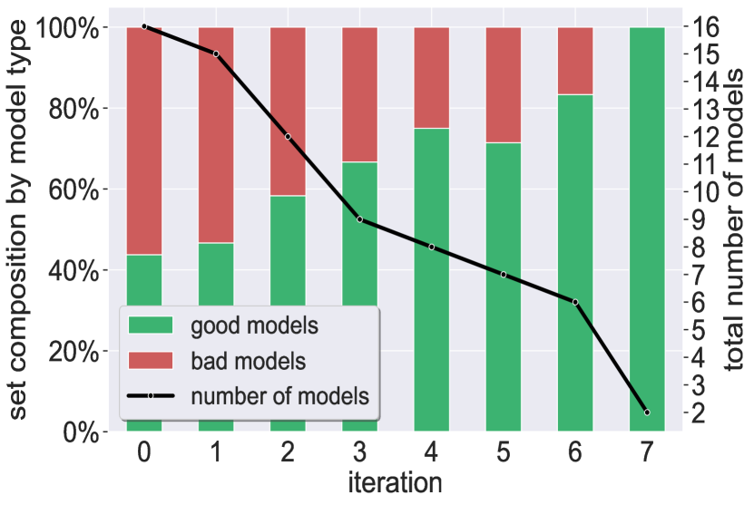
(b) Remaining good and bad models ratio

Figure 28: Aurora Experiment 4.3: results using the MAX filtering criterion.

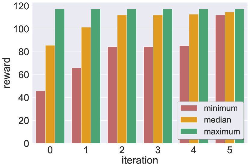
(a) Rewards statistics

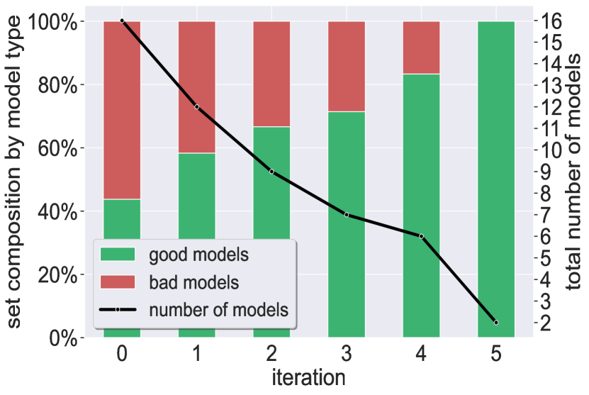
(b) Remaining good and bad models ratio

Figure 29: Aurora Experiment 4.3: results using the COMBINED filtering criterion.

F.4 Additional Filtering Criteria: Experiment 20

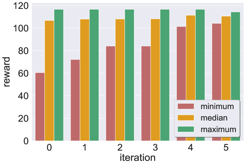
(a) Rewards statistics

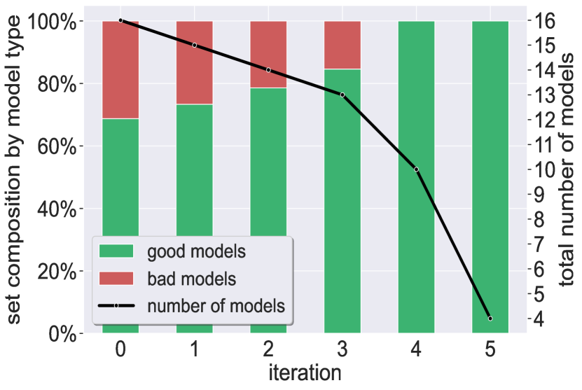
(b) Remaining good and bad models ratio

Figure 30: Aurora Experiment 20: results using the MAX filtering criterion.

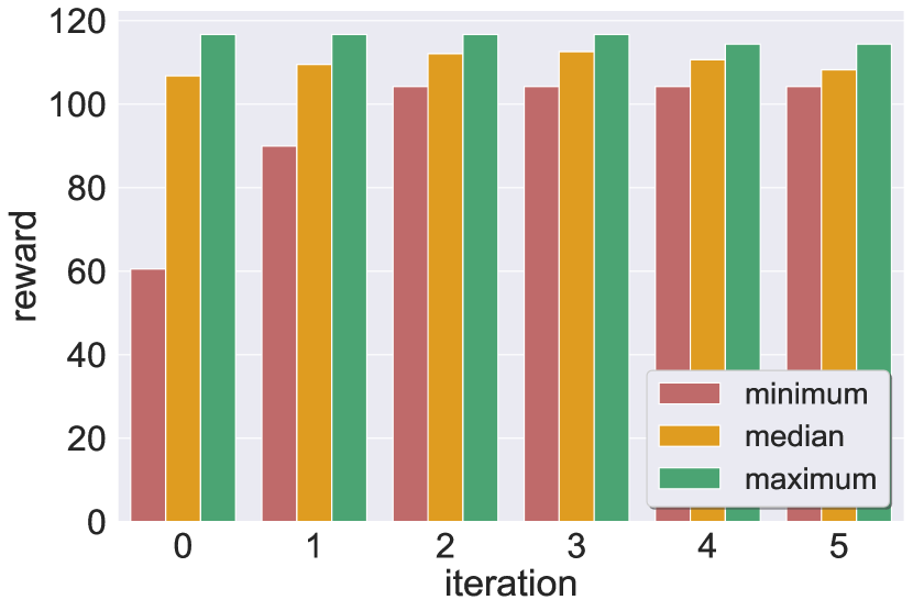
(a) Rewards statistics

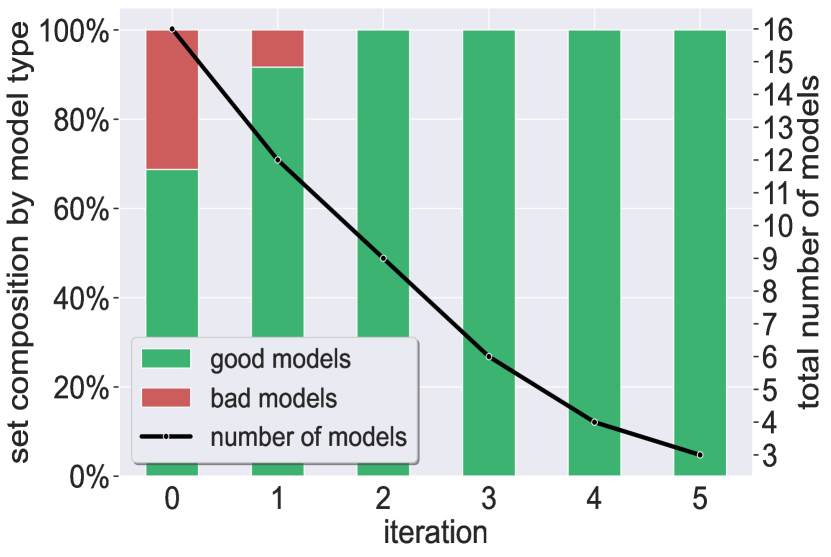
(b) Remaining good and bad models ratio

Figure 31: Aurora Experiment 20: results using the COMBINED filtering criterion.

F.5 Additional Filtering Criteria: Additional PDFs

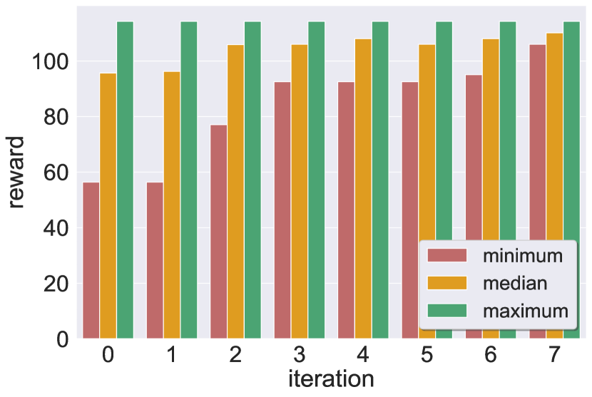
(a) Rewards statistics

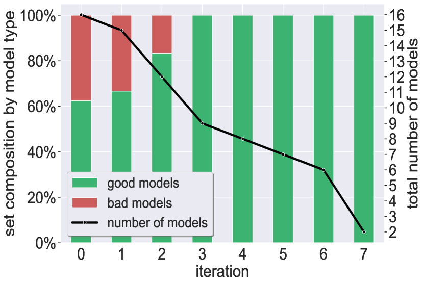
(b) Remaining good and bad models ratio

Figure 32: Aurora Experiment 4.3: PDF $\sim\mathcal{TN}(\mu_{low},\sigma^{2}$): results using the MAX filtering criterion.

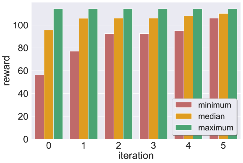
(a) Rewards statistics

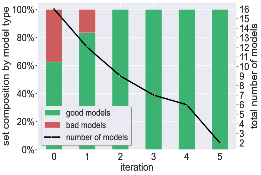
(b) Remaining good and bad models ratio

Figure 33: Aurora Experiment 4.3: PDF $\sim\mathcal{TN}(\mu_{low},\sigma^{2}$): results using the COMBINED filtering criterion.

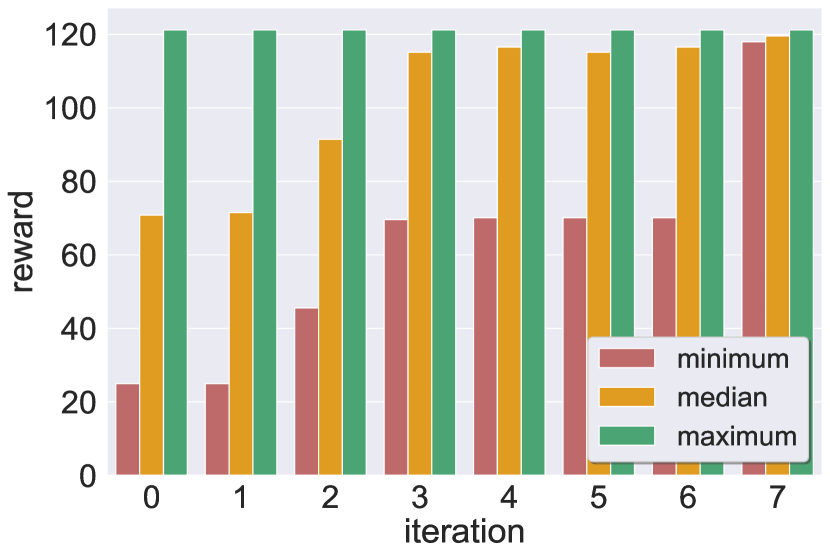
(a) Rewards statistics

(b) Remaining good and bad models ratio

Figure 34: Aurora Experiment 4.3: PDF $\sim\mathcal{TN}(\mu_{high},\sigma^{2}$): results using the MAX filtering criterion.

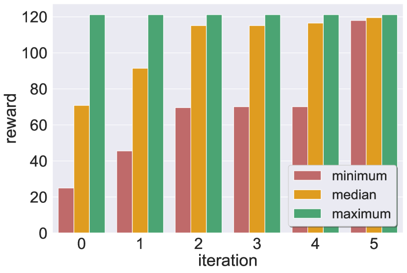
(a) Rewards statistics

(b) Remaining good and bad models ratio

Figure 35: Aurora Experiment 4.3: PDF $\sim\mathcal{TN}(\mu_{high},\sigma^{2}$): results using the COMBINED filtering criterion.

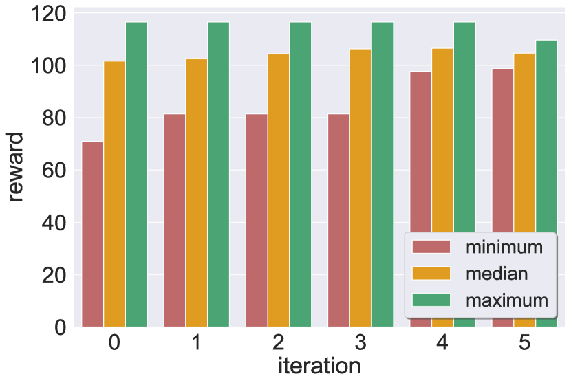
(a) Rewards statistics

(b) Remaining good and bad models ratio

Figure 36: Aurora Experiment 20:, PDF $\sim\mathcal{TN}(\mu_{low},\sigma^{2}$): results using the MAX filtering criterion.

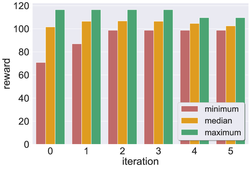
(a) Rewards statistics

(b) Remaining good and bad models ratio

Figure 37: Aurora Experiment 20: PDF $\sim\mathcal{TN}(\mu_{low},\sigma^{2}$): results using the COMBINED filtering criterion.

(a) Rewards statistics

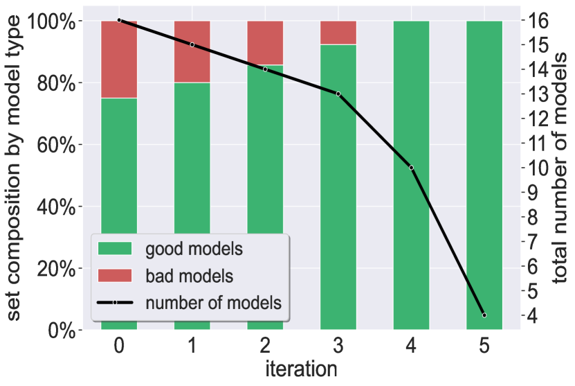
(b) Remaining good and bad models ratio

Figure 38: Aurora Experiment 20: PDF $\sim\mathcal{TN}(\mu_{high},\sigma^{2}$): results using the MAX filtering criterion.

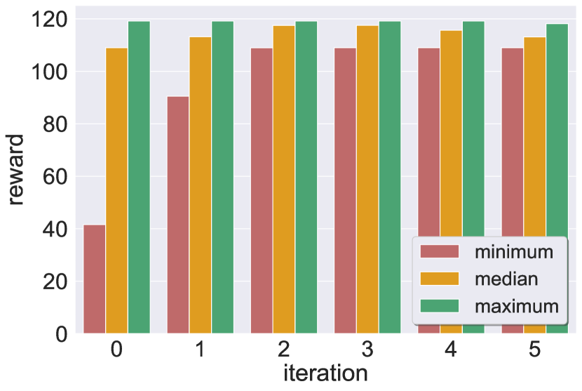
(a) Rewards statistics

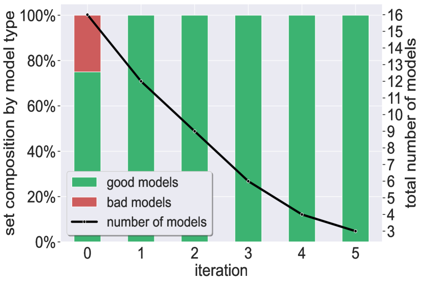
(b) Remaining good and bad models ratio

Figure 39: Aurora Experiment 20: PDF $\sim\mathcal{TN}(\mu_{high},\sigma^{2}$): results using the COMBINED filtering criterion.

Appendix G Comparison to Gradient-Based Methods

G.1 Introduction

The methods presented in this paper effectively utilize DNN verification technology (Line 4 in Alg. 1) in order to solve an optimization problem: given a pair of DNNs, a predefined inputs domain, and a distance function, what is the maximal distance between their outputs? In other words, we use verification to find an input that maximizes the difference between the outputs of two neural networks, under certain constraints. Although verification is highly complex [53], we demonstrate that it is crucial in our setting. Specifically, we show the results of our method when verification is replaced with other techniques. One such technique for optimizing non-convex functions is utilizing gradient-based algorithms (“attacks”) such as Gradient Descent [90], Projected Gradient Descent (PGD) [69], and others. These methods, however, are not directly suitable for optimizing non-trivial constraints, and hence require modification in order for them to succeed in our scenarios (see “distance functions” in Appendix B). We generated three gradient attacks:

1. gradient attack # 1: a non-iterative Fast Gradient Sign Method (FGSM) [46] attack, used when optimizing linear constraints (i.e., $L_{1}$ norm; see Appendix B), as in the case of Aurora.

2. gradient attack # 2: an Iterative PGD [69] attack, also used when optimizing linear constraints (i.e., $L_{1}$ norm; see Appendix B), as in the case of Aurora. We note that we used this attack in cases when the previous attack failed on linear constraints.

3. gradient attack # 3: a Constrained Iterative PGD [69] attack, used in the case when encoding non-linear constraints (i.e., c-distance function; see Appendix B), as in the case of Cartpole and Mountain Car.

Next, we formalize these constrained optimization problems.

G.2 Formulation

Throughout our work, we focus on an output space $\mathcal{O}=\mathbb{R}$. For a shared input domain $\mathcal{D}$ and two neural networks $N_{1}:\mathcal{D}\to\mathbb{R}$ and $N_{2}:\mathcal{D}\to\mathbb{R}$, for which we wish to find an input $\boldsymbol{x}\in\mathcal{D}$ that maximizes the difference between the outputs of these neural networks.

Formally, in the case of the $L_{1}$ norm, we wish to solve the following optimization problem:

$$\underset{x}{\textbf{max}}\quad |N_{1}(\boldsymbol{x})-N_{2}(\boldsymbol{x})|$$

s.t. $$\boldsymbol{x}\in\mathcal{D}$$

G.2.1 Gradient Attacks $1$ & $2$.

When only input constraints are present, a local maximum can be obtained via conventional gradient methods, maximizing the following objective function:

$$L(\boldsymbol{x})=|N_{1}(\boldsymbol{x})-N_{2}(\boldsymbol{x})|$$

by taking steps in the direction of its gradient, and projecting them into the domain $\mathcal{D}$, that is:

$$\boldsymbol{x_{0}}\in\mathcal{D}$$

$$\boldsymbol{x}_{t+1}=[\boldsymbol{x}_{t}+\epsilon\cdot\nabla_{\boldsymbol{x}}L(\boldsymbol{x}_{t})]_{\mathcal{D}}$$

Where $[\cdot]_{\mathcal{D}}:\mathbb{R}^{n}\to\mathcal{D}$ projects the result onto $\mathcal{D}$ and $\epsilon$ is the step size. we note that $[\cdot]_{\mathcal{D}}$ may not be trivial to implement, however for $\mathcal{D}\equiv\{\boldsymbol{x}\ |\ x\in\mathbb{R}^{n}\,\,\forall i\in[n]:l_{i}\leq x_{i}\leq u_{i}\}$ it can be implemented by clipping every coordinate to its appropriate range and $\boldsymbol{x_{0}}$ can be obtained by taking $\boldsymbol{x_{0}}=\frac{\boldsymbol{l}+\boldsymbol{u}}{2}$.

For adversarial attacks on DNNs, i.e., maximizing a loss function for a pair of DNNs, relative to their input, the FGSM algorithm (gradient attack # 1) moves in a single step toward the direction of the gradient. This simple attack has been shown [46] to be quite efficient for causing misclassification. This (projected) FGSM is formalized as follows:

Algorithm 3 FGSM

Input: objective $L$, variables $\boldsymbol{x}$, input domain $\mathcal{D}$:(INIT, PROJECT), step size $\epsilon$
      Output: adversarial input $\boldsymbol{x}$

1:$\boldsymbol{x_{0}}\leftarrow\textsc{Init}(\mathcal{D})$

2:$\boldsymbol{x}_{\textbf{adv}}\leftarrow\textsc{Project}(\boldsymbol{x}_{0}+\epsilon\cdot\textbf{sign}(\nabla_{\boldsymbol{x}}L(\boldsymbol{x}_{0})))$

3:return $\boldsymbol{x}_{\textbf{adv}}$

In the context of our algorithms, we define $\mathcal{D}$ by two functions: INIT which returns an initial value from $\mathcal{D}$ and PROJECT which implements $[\cdot]_{\mathcal{D}}$.

A more powerful extension of this attack is the PGD algorithm, which we refer to as gradient attack # 2. This attack iteratively moves in the direction of the gradient, often yielding superior results when compared to its single-step counterpart. The attack is formalized as follows:

Algorithm 4 PGD (maximize)

Input: objective $L$, variables $\boldsymbol{x}$, input domain $\mathcal{D}$:(INIT, PROJECT), iterations $T$, step size $\epsilon$
      Output: adversarial input $\boldsymbol{x}$

1:$\boldsymbol{x_{0}}\leftarrow\texttt{INIT}({\mathcal{D}})$

2:for $t=0\ldots T-1$ do

3:     $\boldsymbol{x}_{t+1}\leftarrow\texttt{PROJECT}({\boldsymbol{x}_{t}+\epsilon\cdot\nabla_{\boldsymbol{x}}L(\boldsymbol{x}_{t})})$ $\triangleright$ $\textbf{sign}(\nabla_{\boldsymbol{x}}L(\boldsymbol{x}_{t}))$ may also be used

4:end for

5:return $\boldsymbol{x}_{T}$

We note that the case for using PGD in order to minimize the objective function is symmetric.

G.2.2 Gradient Attack $3$.

However, in some cases, the gradient attack needs to optimize a loss function that represents constraints on the outputs of the DNN pairs as well. This is the case with the Cartpole and Mountain Car benchmarks, in which we used the c-distance function. Specifically, in this scenario, we may need to encode constraints of the form:

$$N_{1}(\boldsymbol{x})\leq 0$$

$$N_{2}(\boldsymbol{x})\leq 0$$

resulting in the following constrained optimization problem:

$$\underset{x}{\textbf{max}}\quad |N_{1}(\boldsymbol{x})-N_{2}(\boldsymbol{x})|$$

s.t. $$\boldsymbol{x}\in\mathcal{D}$$

$$N_{1}(\boldsymbol{x})\leq 0$$

$$N_{2}(\boldsymbol{x})\leq 0$$

Conventional gradient attacks are typically not used to solve such optimizations. Hence, we tailored an additional gradient attack (gradient attack # 3) that can efficiently do so by combining our Iterative PGD attack with Lagrange Multipliers [87] $\boldsymbol{\lambda}\equiv(\lambda^{(1)},\lambda^{(2)})$ to penalize solutions for which the constraints do not hold. To this end, we defined a novel objective function:

$$L_{-}(\boldsymbol{x},\boldsymbol{\lambda})=|N_{1}(\boldsymbol{x})-N_{2}(\boldsymbol{x})|-\lambda^{(1)}\cdot\text{ReLU}(N_{1}(\boldsymbol{x}))-\lambda^{(2)}\cdot\text{ReLU}(N_{2}(\boldsymbol{x}))$$

resulting in the following optimization problem:

$$\underset{x}{\textbf{max}}\,\underset{\lambda}{\textbf{min}}\quad L_{-}(\boldsymbol{x},\boldsymbol{\lambda})$$

s.t. $$\boldsymbol{x}\in\mathcal{D}$$

$$\lambda^{(1)}\geq 0$$

$$\lambda^{(2)}\geq 0$$

and implemented a Constrained Iterative PGD algorithm that approximates a solution:

Algorithm 5 Constrained Iterative PGD

Input: objective $L$, input domain $\mathcal{D}$, constraints: $C_{i}(\boldsymbol{x})$, iterations: $T,T_{x},T_{\lambda}$, step sizes: $\epsilon_{x},\epsilon_{\lambda}$
      Output: adversarial input $\boldsymbol{x}$

$\boldsymbol{x_{0}}\leftarrow\textsc{Init}(\mathcal{D})$

$L_{C}(\boldsymbol{x},\boldsymbol{\lambda})\equiv L(\boldsymbol{x})-\sum^{k}_{i=0}\lambda^{(i)}\cdot\text{ReLU}(C_{i}(\boldsymbol{x}))$ $\triangleright$ the new objective

for $t=0\ldots T-1$ do

     $\boldsymbol{\lambda}_{t+1}\leftarrow\textsc{PGD\_min}(L_{C},\boldsymbol{\lambda},(\boldsymbol{\lambda}\leftarrow 0,\boldsymbol{\lambda}\geq 0),T_{\lambda},\epsilon_{\lambda})$ $\triangleright$ minimize $L_{C}(\boldsymbol{x}_{t},\boldsymbol{\lambda})$ with $\boldsymbol{x}_{t}$ as constant

     $\boldsymbol{x}_{t+1}\leftarrow\textsc{PGD\_max}(L_{C},\boldsymbol{x},\mathcal{D},T_{x},\epsilon_{x})$ $\triangleright$ maximize $L_{C}(\boldsymbol{x},\boldsymbol{\lambda}_{t})$ with $\boldsymbol{\lambda}_{t}$ as constant

end for

return $\boldsymbol{x}_{T}$

G.3 Results

As elaborated in subsection 4.4, we ran our algorithm on the original models, with the sole difference being the replacement of the backend verification engine (Line 4 in Alg. 1) with the attacks described above. The first two attacks (i.e., FGSM and Iterative PGD) were used for both Aurora batches (“short” and “long” training), and the third (Constrained Iterative PGD) was used in the case of Cartpole and Mountain Car. We note that in the case of Aurora, we ran the Iterative PGD attack only when the weaker attack failed (hence, only the models from Experiment 4.3). The results (summarized in Table 5) validate that in the majority of the cases, the attack either failed or mistakenly recognized bad models as good ones in the predefined input region. For further details regarding the cases in which the feasible gradient attacks failed, see Fig. 40, Fig. 41, and Fig. 42. These results show the importance of using verification for our method.

ATTACK	BENCHMARK	FEASIBLE	$\#$ PAIRS	$\#$ ALIGNED	$\#$ UNTIGHTENED	$\#$ FAILED	CRITERION	SUCCESSFUL
1	Aurora (short)	yes	120	70	50	0	MAX	no
							COMBINED	yes
							PERCENTILE	yes
1	Aurora (long)	yes	120	111	9	0	MAX	yes
							COMBINED	yes
							PERCENTILE	yes
2	Aurora (short)	yes	120	104	16	0	MAX	no
							COMBINED	yes
							PERCENTILE	yes
3	Mountain Car	no	120	38	35	47	MAX	no
							COMBINED	no
							PERCENTILE	no
3	Cartpole	partially	120	56	61	3	MAX	no
							PERCENTILE	no
							PERCENTILE	no

Table 5: Summary of the gradient attack comparison. The first two columns describe the attack chosen and the benchmark on which it was evaluated; the third column states if the incomplete attack allowed a gradient-based approximation of all PDT scores; the next four columns respectively represent the total number of DNN pairs, the number of pairs in which the attack returned a PDT score identical to the original one received by our verification engine, the number of pairs in which the attack returned a score that is less precise than the one returned by our verification engine; and the number of cases in which that attack failed. The second-to-last column shows the filtering criterion, and the last column indicates whether using the attack-based scores resulted in good models only (as was the case when verification was used).

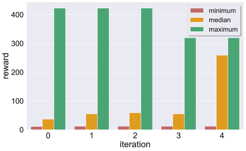
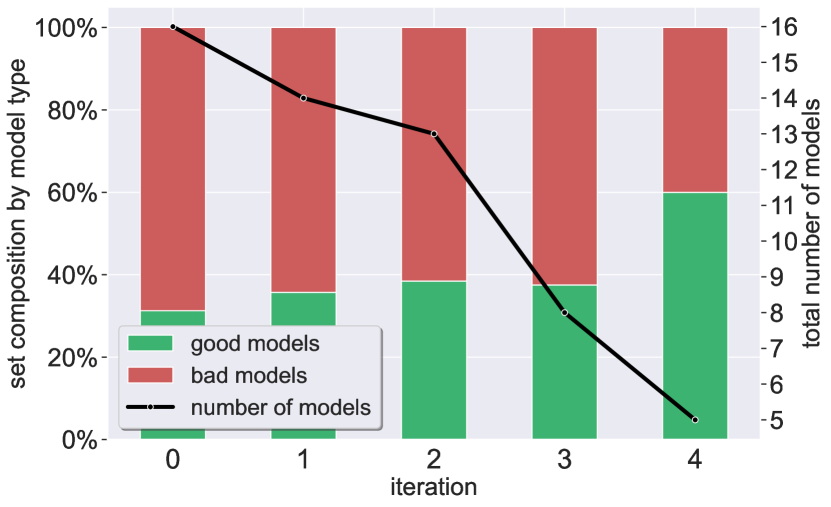
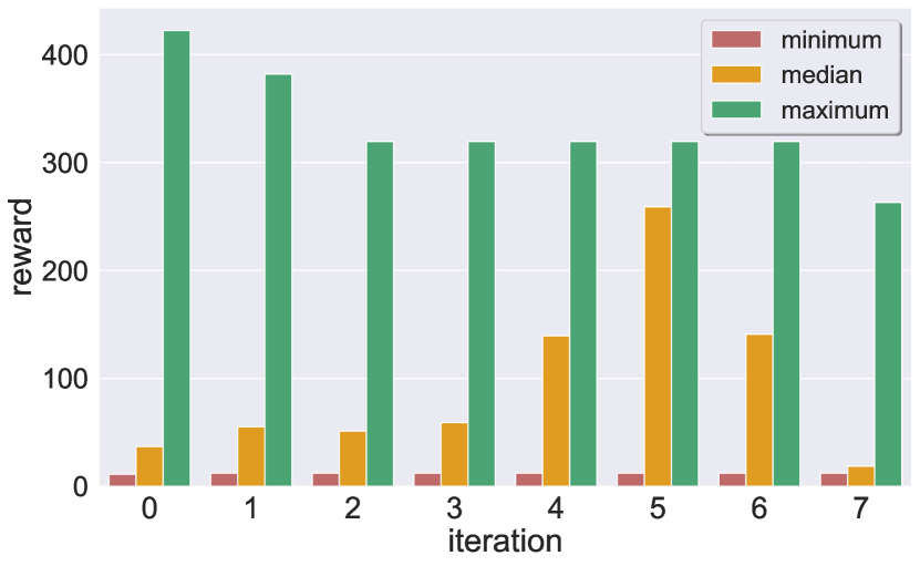
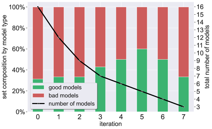
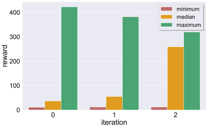
(a) Rewards statistics

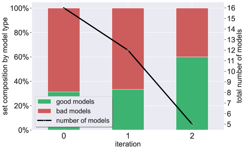
(b) Remaining good and bad models ratio

Figure 40: Cartpole: attack # 3 (Constrained Iterative PGD): Results of models filtered using PDT scores approximated by gradient attacks (instead of a verification engine) on the Cartpole models.
Each row, from top to bottom, contains results using a different filtering criterion (and terminating in advance if the disagreement scores are no larger than $2$): PERCENTILE (compare to Fig. 3 and Fig. 10), MAX (compare to Fig. 11), and COMBINED (compare to Fig. 12).
In all cases, the algorithm returns at least one bad model (and usually more than one), resulting in models with lower average rewards than our verification-based results.

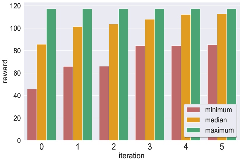
(a) Rewards statistics

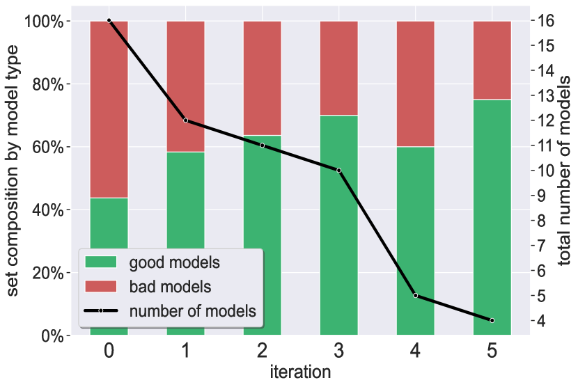
(b) Remaining good and bad models ratio

Figure 41: Aurora: attack # 1 (single-step FGSM): Results of models filtered using PDT scores approximated by gradient attacks (instead of a verification engine) on short-trained Aurora models, using the MAX criterion (and terminating in advance if the disagreement scores are no larger than $2$). In contrast to our verification-driven approach, the final result contains a bad model. Compare to Fig. 28.

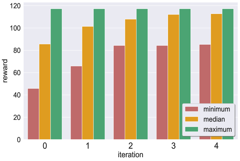
(a) Rewards statistics

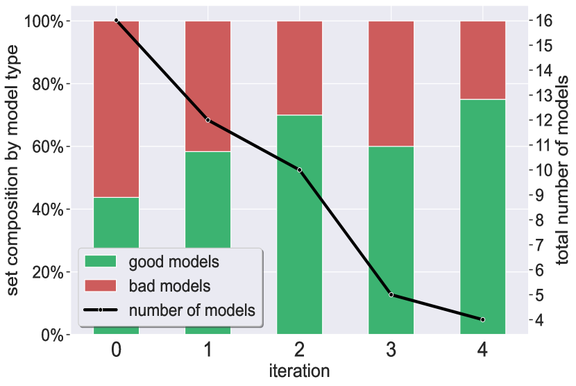
(b) Remaining good and bad models ratio

Figure 42: Aurora: attack # 2 (Iterative PGD): Results of models filtered using PDT scores approximated by gradient attacks (instead of a verification engine) on short-trained Aurora models, using the MAX criterion (and terminating in advance if the disagreement scores are no larger than $2$). In contrast to our verification-driven approach, the final result contains a bad model. Compare to Fig. 28.

References

- [1] M. Abdar, F. Pourpanah, S. Hussain, D. Rezazadegan, L. Liu, M. Ghavamzadeh, P. Fieguth, X. Cao, A. Khosravi, U. Acharya, V. Makarenkov, and S. Nahavandi. A Review of Uncertainty Quantification in Deep Learning: Techniques, Applications and Challenges. Information Fusion, 76:243–297, 2021.
- [2] P. Alamdari, G. Avni, T. Henzinger, and A. Lukina. Formal Methods with a Touch of Magic. In Proc. 20th Int. Conf. on Formal Methods in Computer-Aided Design (FMCAD), pages 138–147, 2020.
- [3] A. Albarghouthi. Introduction to Neural Network Verification. verifieddeeplearning.com, 2021.
- [4] M. AlQuraishi. AlphaFold at CASP13. Bioinformatics, 35(22):4862–4865, 2019.
- [5] G. Amir, D. Corsi, R. Yerushalmi, L. Marzari, D. Harel, A. Farinelli, and G. Katz. Verifying Learning-Based Robotic Navigation Systems. In Proc. 29th Int. Conf. on Tools and Algorithms for the Construction and Analysis of Systems (TACAS), pages 607–627, 2023.
- [6] G. Amir, Z. Freund, G. Katz, E. Mandelbaum, and I. Refaeli. veriFIRE: Verifying an Industrial, Learning-Based Wildfire Detection System. In Proc. 25th Int. Symposium on Formal Methods (FM), pages 648–656, 2023.
- [7] G. Amir, O. Maayan, T. Zelazny, G. Katz, and M. Schapira. Verifying Generalization in Deep Learning: Artifact, 2023. https://zenodo.org/record/7884514#.ZFAz_3ZBy3B.
- [8] G. Amir, M. Schapira, and G. Katz. Towards Scalable Verification of Deep Reinforcement Learning. In Proc. 21st Int. Conf. on Formal Methods in Computer-Aided Design (FMCAD), pages 193–203, 2021.
- [9] G. Amir, H. Wu, C. Barrett, and G. Katz. An SMT-Based Approach for Verifying Binarized Neural Networks. In Proc. 27th Int. Conf. on Tools and Algorithms for the Construction and Analysis of Systems (TACAS), pages 203–222, 2021.
- [10] G. Amir, T. Zelazny, G. Katz, and M. Schapira. Verification-Aided Deep Ensemble Selection. In Proc. 22nd Int. Conf. on Formal Methods in Computer-Aided Design (FMCAD), pages 27–37, 2022.
- [11] G. Anderson, S. Pailoor, I. Dillig, and S. Chaudhuri. Optimization and Abstraction: a Synergistic Approach for Analyzing Neural Network Robustness. In Proc. 40th ACM SIGPLAN Conf. on Programming Languages Design and Implementations (PLDI), pages 731–744, 2019.
- [12] P. Ashok, V. Hashemi, J. Kretinsky, and S. Mohr. DeepAbstract: Neural Network Abstraction for Accelerating Verification. In Proc. 18th Int. Symp. on Automated Technology for Verification and Analysis (ATVA), pages 92–107, 2020.
- [13] G. Avni, R. Bloem, K. Chatterjee, T. Henzinger, B. Könighofer, and S. Pranger. Run-Time Optimization for Learned Controllers through Quantitative Games. In Proc. 31st Int. Conf. on Computer Aided Verification (CAV), pages 630–649, 2019.
- [14] E. Bacci, M. Giacobbe, and D. Parker. Verifying Reinforcement Learning up to Infinity. In Proc. 30th Int. Joint Conf. on Artificial Intelligence (IJCAI), 2021.
- [15] T. Baluta, S. Shen, S. Shinde, K. Meel, and P. Saxena. Quantitative Verification of Neural Networks and its Security Applications. In Proc. ACM SIGSAC Conf. on Computer and Communications Security (CCS), pages 1249–1264, 2019.
- [16] A. Barto, R. Sutton, and C. Anderson. Neuronlike Adaptive Elements that Can Solve Difficult Learning Control Problems. In Proc. of IEEE Systems Man and Cybernetics Conference (SMC), pages 834–846, 1983.
- [17] S. Bassan and G. Katz. Towards Formal Approximated Minimal Explanations of Neural Networks. In Proc. 29th Int. Conf. on Tools and Algorithms for the Construction and Analysis of Systems (TACAS), pages 187–207, 2023.
- [18] M. Bojarski, D. Del Testa, D. Dworakowski, B. Firner, B. Flepp, P. Goyal, L. Jackel, M. Monfort, U. Muller, J. Zhang, X. Zhang, J. Zhao, and K. Zieba. End to End Learning for Self-Driving Cars, 2016. Technical Report. http://arxiv.org/abs/1604.07316.
- [19] G. Brockman, V. Cheung, L. Pettersson, J. Schneider, J. Schulman, J. Tang, and W. Zaremba. OpenAI Gym, 2016. Technical Report. https://arxiv.org/abs/1606.01540.
- [20] R. Bunel, I. Turkaslan, P. Torr, P. Kohli, and P. Mudigonda. A Unified View of Piecewise Linear Neural Network Verification. In Proc. 32nd Conf. on Neural Information Processing Systems (NeurIPS), pages 4795–4804, 2018.
- [21] M. Casadio, E. Komendantskaya, M. Daggitt, W. Kokke, G. Katz, G. Amir, and I. Refaeli. Neural Network Robustness as a Verification Property: A Principled Case Study. In Proc. 34th Int. Conf. on Computer Aided Verification (CAV), pages 219–231, 2022.
- [22] W. Chen, Y. Xu, and X. Wu. Deep Reinforcement Learning for Multi-Resource Multi-Machine Job Scheduling, 2017. Technical Report. http://arxiv.org/abs/1711.07440.
- [23] E. Cohen, Y. Elboher, C. Barrett, and G. Katz. Tighter Abstract Queries in Neural Network Verification. In Proc. 24th Int. Conf. on Logic for Programming, Artificial Intelligence and Reasoning (LPAR), 2023.
- [24] R. Collobert, J. Weston, L. Bottou, M. Karlen, K. Kavukcuoglu, and P. Kuksa. Natural Language Processing (Almost) from Scratch. Journal of Machine Learning Research (JMLR), 12:2493–2537, 2011.
- [25] D. Corsi, E. Marchesini, and A. Farinelli. Formal Verification of Neural Networks for Safety-Critical Tasks in Deep Reinforcement Learning. In Proc. 37th Conf. on Uncertainty in Artificial Intelligence (UAI), pages 333–343, 2021.
- [26] D. Corsi, R. Yerushalmi, G. Amir, A. Farinelli, D. Harel, and G. Katz. Constrained Reinforcement Learning for Robotics via Scenario-Based Programming, 2022. Technical Report. https://arxiv.org/abs/2206.09603.
- [27] T. Dietterich. Ensemble Methods in Machine Learning. In Proc. 1st Int. Workshop on Multiple Classifier Systems (MCS), pages 1–15, 2020.
- [28] G. Dong, J. Sun, J. Wang, X. Wang, and T. Dai. Towards Repairing Neural Networks Correctly, 2020. Technical Report. http://arxiv.org/abs/2012.01872.
- [29] S. Dutta, X. Chen, and S. Sankaranarayanan. Reachability Analysis for Neural Feedback Systems using Regressive Polynomial Rule Inference. In Proc. 22nd ACM Int. Conf. on Hybrid Systems: Computation and Control (HSCC), pages 157–168, 2019.
- [30] S. Dutta, S. Jha, S. Sankaranarayanan, and A. Tiwari. Learning and Verification of Feedback Control Systems using Feedforward Neural Networks. IFAC-PapersOnLine, 51(16):151–156, 2018.
- [31] R. Ehlers. Formal Verification of Piece-Wise Linear Feed-Forward Neural Networks. In Proc. 15th Int. Symp. on Automated Technology for Verification and Analysis (ATVA), pages 269–286, 2017.
- [32] Y. Elboher, E. Cohen, and G. Katz. Neural Network Verification using Residual Reasoning. In Proc. 20th Int. Conf. on Software Engineering and Formal Methods (SEFM), pages 173–189, 2022.
- [33] Y. Elboher, J. Gottschlich, and G. Katz. An Abstraction-Based Framework for Neural Network Verification. In Proc. 32nd Int. Conf. on Computer Aided Verification (CAV), pages 43–65, 2020.
- [34] T. Eliyahu, Y. Kazak, G. Katz, and M. Schapira. Verifying Learning-Augmented Systems. In Proc. Conf. of the ACM Special Interest Group on Data Communication on the Applications, Technologies, Architectures, and Protocols for Computer Communication (SIGCOMM), pages 305–318, 2021.
- [35] N. Fulton and A. Platzer. Safe Reinforcement Learning via Formal Methods: Toward Safe Control through Proof and Learning. In Proc. 32nd AAAI Conf. on Artificial Intelligence (AAAI), 2018.
- [36] M. Ganaie, M. Hu, A. Malik, M. Tanveer, and P. Suganthan. Ensemble Deep Learning: A Review. Engineering Applications of Artificial Intelligence, 115:105151, 2022.
- [37] T. Gehr, M. Mirman, D. Drachsler-Cohen, E. Tsankov, S. Chaudhuri, and M. Vechev. AI2: Safety and Robustness Certification of Neural Networks with Abstract Interpretation. In Proc. 39th IEEE Symposium on Security and Privacy (S&P), 2018.
- [38] C. Geng, N. Le, X. Xu, Z. Wang, A. Gurfinkel, and X. Si. Toward Reliable Neural Specifications, 2022. Technical Report. https://arxiv.org/abs/2210.16114.
- [39] S. Geva and J. Sitte. A Cartpole Experiment Benchmark for Trainable Controllers. IEEE Control Systems Magazine, 13(5):40–51, 1993.
- [40] B. Goldberger, Y. Adi, J. Keshet, and G. Katz. Minimal Modifications of Deep Neural Networks using Verification. In Proc. 23rd Int. Conf. on Logic for Programming, Artificial Intelligence and Reasoning (LPAR), pages 260–278, 2020.
- [41] I. Goodfellow, Y. Bengio, and A. Courville. Deep Learning. MIT Press, 2016.
- [42] D. Gopinath, G. Katz, C. Pǎsǎreanu, and C. Barrett. DeepSafe: A Data-driven Approach for Assessing Robustness of Neural Networks. In Proc. 16th. Int. Symposium on Automated Technology for Verification and Analysis (ATVA), pages 3–19, 2018.
- [43] E. Goubault, S. Palumby, S. Putot, L. Rustenholz, and S. Sankaranarayanan. Static Analysis of ReLU Neural Networks with Tropical Polyhedra. In Proc. 28th Int. Symposium on Static Analysis (SAS), pages 166–190, 2021.
- [44] T. Haarnoja, A. Zhou, P. Abbeel, and S. Levine. Soft Actor-Critic: Off-Policy Maximum Entropy Deep Reinforcement Learning with a Stochastic Actor. In Int. Conf. on Machine Learning, pages 1861–1870. PMLR, 2018.
- [45] V. Hashemi, J. Křetínsky, S. Rieder, and J. Schmidt. Runtime Monitoring for Out-of-Distribution Detection in Object Detection Neural Networks, 2022. Technical Report. http://arxiv.org/abs/2212.07773.
- [46] S. Huang, N. Papernot, I. Goodfellow, Y. Duan, and P. Abbeel. Adversarial Attacks on Neural Network Policies, 2017. Technical Report. https://arxiv.org/abs/1702.02284.
- [47] X. Huang, M. Kwiatkowska, S. Wang, and M. Wu. Safety Verification of Deep Neural Networks. In Proc. 29th Int. Conf. on Computer Aided Verification (CAV), pages 3–29, 2017.
- [48] O. Isac, C. Barrett, M. Zhang, and G. Katz. Neural Network Verification with Proof Production. In Proc. 22nd Int. Conf. on Formal Methods in Computer-Aided Design (FMCAD), pages 38–48, 2022.
- [49] Y. Jacoby, C. Barrett, and G. Katz. Verifying Recurrent Neural Networks using Invariant Inference. In Proc. 18th Int. Symposium on Automated Technology for Verification and Analysis (ATVA), pages 57–74, 2020.
- [50] N. Jay, N. Rotman, B. Godfrey, M. Schapira, and A. Tamar. A Deep Reinforcement Learning Perspective on Internet Congestion Control. In Proc. 36th Int. Conf. on Machine Learning (ICML), pages 3050–3059, 2019.
- [51] K. Julian, J. Lopez, J. Brush, M. Owen, and M. Kochenderfer. Policy Compression for Aircraft Collision Avoidance Systems. In Proc. 35th Digital Avionics Systems Conf. (DASC), pages 1–10, 2016.
- [52] G. Katz, C. Barrett, D. Dill, K. Julian, and M. Kochenderfer. Reluplex: An Efficient SMT Solver for Verifying Deep Neural Networks. In Proc. 29th Int. Conf. on Computer Aided Verification (CAV), pages 97–117, 2017.
- [53] G. Katz, C. Barrett, D. Dill, K. Julian, and M. Kochenderfer. Reluplex: a Calculus for Reasoning about Deep Neural Networks. Formal Methods in System Design (FMSD), 2021.
- [54] G. Katz, D. Huang, D. Ibeling, K. Julian, C. Lazarus, R. Lim, P. Shah, S. Thakoor, H. Wu, A. Zeljić, D. Dill, M. Kochenderfer, and C. Barrett. The Marabou Framework for Verification and Analysis of Deep Neural Networks. In Proc. 31st Int. Conf. on Computer Aided Verification (CAV), pages 443–452, 2019.
- [55] B. Könighofer, F. Lorber, N. Jansen, and R. Bloem. Shield Synthesis for Reinforcement Learning. In Proc. Int. Symposium on Leveraging Applications of Formal Methods, Verification and Validation (ISoLA), pages 290–306, 2020.
- [56] A. Krizhevsky, I. Sutskever, and G. Hinton. Imagenet Classification with Deep Convolutional Neural Networks. In Proc. 26th Conf. on Neural Information Processing Systems (NeurIPS), pages 1097–1105, 2012.
- [57] A. Krogh and J. Vedelsby. Neural Network Ensembles, Cross Validation, and Active Learning. In Proc. 7th Conf. on Neural Information Processing Systems (NeurIPS), pages 231–238, 1994.
- [58] L. Kuper, G. Katz, J. Gottschlich, K. Julian, C. Barrett, and M. Kochenderfer. Toward Scalable Verification for Safety-Critical Deep Networks, 2018. Technical Report. https://arxiv.org/abs/1801.05950.
- [59] A. Kurakin, I. Goodfellow, and S. Bengio. Adversarial Examples in the Physical World, 2016. Technical Report. http://arxiv.org/abs/1607.02533.
- [60] A. Lekharu, K. Moulii, A. Sur, and A. Sarkar. Deep Learning Based Prediction Model for Adaptive Video Streaming. In Proc. 12th Int. Conf. on Communication Systems & Networks (COMSNETS), pages 152–159. IEEE, 2020.
- [61] W. Li, F. Zhou, K. R. Chowdhury, and W. Meleis. QTCP: Adaptive Congestion Control with Reinforcement Learning. IEEE Transactions on Network Science and Engineering, 6(3):445–458, 2018.
- [62] Y. Li. Deep Reinforcement Learning: An Overview, 2017. Technical Report. http://arxiv.org/abs/1701.07274.
- [63] A. Lomuscio and L. Maganti. An Approach to Reachability Analysis for Feed-Forward ReLU Neural Networks, 2017. Technical Report. http://arxiv.org/abs/1706.07351.
- [64] A. Loquercio, M. Segu, and D. Scaramuzza. A General Framework for Uncertainty Estimation in Deep Learning. In Proc. Int. Conf. on Robotics and Automation (ICRA), pages 3153–3160, 2020.
- [65] S. Low, F. Paganini, and J. Doyle. Internet Congestion Control. IEEE Control Systems Magazine, 22(1):28–43, 2002.
- [66] A. Lukina, C. Schilling, and T. Henzinger. Into the Unknown: Active Monitoring of Neural Networks. In Proc. 21st Int. Conf. on Runtime Verification (RV), pages 42–61, 2021.
- [67] Z. Lyu, C. Y. Ko, Z. Kong, N. Wong, D. Lin, and L. Daniel. Fastened Crown: Tightened Neural Network Robustness Certificates. In Proc. 34th AAAI Conf. on Artificial Intelligence (AAAI), pages 5037–5044, 2020.
- [68] J. Ma, S. Ding, and Q. Mei. Towards More Practical Adversarial Attacks on Graph Neural Networks. In Proc. 34th Conf. on Neural Information Processing Systems (NeurIPS), 2020.
- [69] A. Madry, A. Makelov, L. Schmidt, D. Tsipras, and A. Vladu. Towards Deep Learning Models Resistant to Adversarial Attacks, 2017. Technical Report. http://arxiv.org/abs/1706.06083.
- [70] R. Mammadli, A. Jannesari, and F. Wolf. Static Neural Compiler Optimization via Deep Reinforcement Learning. In Proc. 6th IEEE/ACM Workshop on the LLVM Compiler Infrastructure in HPC (LLVM-HPC) and Workshop on Hierarchical Parallelism for Exascale Computing (HiPar), pages 1–11, 2020.
- [71] H. Mao, M. Alizadeh, I. Menache, and S. Kandula. Resource Management with Deep Reinforcement Learning. In Proc. 15th ACM Workshop on Hot Topics in Networks (HotNets), pages 50–56, 2016.
- [72] H. Mao, R. Netravali, and M. Alizadeh. Neural Adaptive Video Streaming with Pensieve. In Proc. Conf. of the ACM Special Interest Group on Data Communication on the Applications, Technologies, Architectures, and Protocols for Computer Communication (SIGCOMM), pages 197–210, 2017.
- [73] V. Mnih, K. Kavukcuoglu, D. Silver, A. Graves, I. Antonoglou, D. Wierstra, and M. Riedmiller. Playing Atari with Deep Reinforcement Learning, 2013. Technical Report. https://arxiv.org/abs/1312.5602.
- [74] A. Moore. Efficient Memory-based Learning for Robot Control, 1990. University of Cambridge.
- [75] J. Nagle. Congestion Control in IP/TCP Internetworks. ACM SIGCOMM Computer Communication Review, 14(4):11–17, 1984.
- [76] T. Okudono, M. Waga, T. Sekiyama, and I. Hasuo. Weighted Automata Extraction from Recurrent Neural Networks via Regression on State Spaces. In Proc. 34th AAAI Conf. on Artificial Intelligence (AAAI), pages 5037–5044, 2020.
- [77] L. Ortega, R. Cabañas, and A. Masegosa. Diversity and Generalization in Neural Network Ensembles. In Proc. 25th Int. Conf. on Artificial Intelligence and Statistics (AISTATS), pages 11720–11743, 2022.
- [78] I. Osband, J. Aslanides, and A. Cassirer. Randomized Prior Functions for Deep Reinforcement Learning. In Proc. 31st Int. Conf. on Neural Information Processing Systems (NeurIPS), pages 8617–8629, 2018.
- [79] M. Ostrovsky, C. Barrett, and G. Katz. An Abstraction-Refinement Approach to Verifying Convolutional Neural Networks. In Proc. 20th. Int. Symposium on Automated Technology for Verification and Analysis (ATVA), pages 391–396, 2022.
- [80] Y. Ovadia, E. Fertig, J. Ren, Z. Nado, D. Sculley, S. Nowozin, J. Dillon, B. Lakshminarayanan, and J. Snoek. Can You Trust Your Model’s Uncertainty? Evaluating Predictive Uncertainty Under Dataset Shift. In Proc. 33rd Conf. on Neural Information Processing Systems (NeurIPS), pages 14003–14014, 2019.
- [81] C. Packer, K. Gao, J. Kos, P. Krähenbühl, V. Koltun, and D. Song. Assessing Generalization in Deep Reinforcement Learning, 2018. Technical Report. https://arxiv.org/abs/1810.12282.
- [82] E. Polgreen, R. Abboud, and D. Kroening. Counterexample Guided Neural Synthesis, 2020. Technical Report. https://arxiv.org/abs/2001.09245.
- [83] P. Prabhakar. Bisimulations for Neural Network Reduction. In Proc. 23rd Int. Conf. Verification on Model Checking, and Abstract Interpretation (VMCAI), pages 285–300, 2022.
- [84] P. Prabhakar and Z. Afzal. Abstraction Based Output Range Analysis for Neural Networks, 2020. Technical Report. https://arxiv.org/abs/2007.09527.
- [85] A. Raffin, A. Hill, A. Gleave, A. Kanervisto, M. Ernestus, and N. Dormann. Stable-Baselines3: Reliable Reinforcement Learning Implementations. Journal of Machine Learning Research (JMLR), 22:1–8, 2021.
- [86] M. Riedmiller. Neural Fitted Q Iteration — First Experiences with a Data Efficient Neural Reinforcement Learning Method. In Proc. 16th European Conf. on Machine Learning (ECML), pages 317–328, 2005.
- [87] T. Rockafellar. Lagrange Multipliers and Optimality. SIAM Review, 35(2):183–238, 1993.
- [88] N. Rotman, M. Schapira, and A. Tamar. Online Safety Assurance for Deep Reinforcement Learning. In Proc. 19th ACM Workshop on Hot Topics in Networks (HotNets), pages 88–95, 2020.
- [89] W. Ruan, X. Huang, and M. Kwiatkowska. Reachability Analysis of Deep Neural Networks with Provable Guarantees. In Proc. 27th Int. Joint Conf. on Artificial Intelligence (IJCAI), 2018.
- [90] S. Ruder. An Overview of Gradient Descent Optimization Algorithms, 2016. Technical Report. https://arxiv.org/abs/1609.04747.
- [91] J. Schulman, F. Wolski, P. Dhariwal, A. Radford, and O. Klimov. Proximal Policy Optimization Algorithms, 2017. Technical Report. http://arxiv.org/abs/1707.06347.
- [92] S. Seshia, A. Desai, T. Dreossi, D. Fremont, S. Ghosh, E. Kim, S. Shivakumar, M. Vazquez-Chanlatte, and X. Yue. Formal Specification for Deep Neural Networks. In Proc. 16th Int. Symposium on Automated Technology for Verification and Analysis (ATVA), pages 20–34, 2018.
- [93] D. Silver, A. Huang, C. Maddison, A. Guez, L. Sifre, G. van Den Driessche, J. Schrittwieser, I. Antonoglou, V. Panneershelvam, M. Lanctot, and S. Dieleman. Mastering the Game of Go with Deep Neural Networks and Tree Search. Nature, 529(7587):484–489, 2016.
- [94] K. Simonyan and A. Zisserman. Very Deep Convolutional Networks for Large-Scale Image Recognition, 2014. Technical Report. http://arxiv.org/abs/1409.1556.
- [95] G. Singh, T. Gehr, M. Puschel, and M. Vechev. An Abstract Domain for Certifying Neural Networks. In Proc. 46th ACM SIGPLAN Symposium on Principles of Programming Languages (POPL), 2019.
- [96] M. Sotoudeh and A. Thakur. Correcting Deep Neural Networks with Small, Generalizing Patches. In Workshop on Safety and Robustness in Decision Making, 2019.
- [97] C. Strong, H. Wu, A. Zeljić, K. Julian, G. Katz, C. Barrett, and M. Kochenderfer. Global Optimization of Objective Functions Represented by ReLU Networks. Journal of Machine Learning, pages 1–28, 2021.
- [98] X. Sun, H. Khedr, and Y. Shoukry. Formal Verification of Neural Network Controlled Autonomous Systems. In Proc. 22nd ACM Int. Conf. on Hybrid Systems: Computation and Control (HSCC), 2019.
- [99] R. Sutton and A. Barto. Reinforcement Learning: An Introduction. MIT press, 2018.
- [100] R. Sutton, D. McAllester, S. Singh, and Y. Mansour. Policy Gradient Methods for Reinforcement Learning with Function Approximation. In Proc. 12th Conf. on Neural Information Processing Systems (NeurIPS), 1999.
- [101] V. Tjeng, K. Xiao, and R. Tedrake. Evaluating Robustness of Neural Networks with Mixed Integer Programming, 2017. Technical Report. http://arxiv.org/abs/1711.07356.
- [102] L. Tolstoy. Anna Karenina. The Russian Messenger, 1877.
- [103] C. Urban, M. Christakis, V. Wüstholz, and F. Zhang. Perfectly Parallel Fairness Certification of Neural Networks. In Proc. ACM Int. Conf. on Object Oriented Programming Systems Languages and Applications (OOPSLA), pages 1–30, 2020.
- [104] M. Usman, D. Gopinath, Y. Sun, Y. Noller, and C. Pǎsǎreanu. NNrepair: Constraint-based Repair of Neural Network Classifiers, 2021. Technical Report. http://arxiv.org/abs/2103.12535.
- [105] A. Valadarsky, M. Schapira, D. Shahaf, and A. Tamar. Learning to Route with Deep RL. In NeurIPS Deep Reinforcement Learning Symposium, 2017.
- [106] H. van Hasselt, A. Guez, and D. Silver. Deep Reinforcement Learning with Double Q-Learning. In Proc. 30th AAAI Conf. on Artificial Intelligence (AAAI), 2016.
- [107] M. Vasić, A. Petrović, K. Wang, M. Nikolić, R. Singh, and S. Khurshid. MoËT: Mixture of Expert Trees and its Application to Verifiable Reinforcement Learning. Neural Networks, 151:34–47, 2022.
- [108] S. Wang, K. Pei, J. Whitehouse, J. Yang, and S. Jana. Formal Security Analysis of Neural Networks using Symbolic Intervals. In Proc. 27th USENIX Security Symposium, pages 1599–1614, 2018.
- [109] H. Wu, A. Ozdemir, A. Zeljić, A. Irfan, K. Julian, D. Gopinath, S. Fouladi, G. Katz, C. Păsăreanu, and C. Barrett. Parallelization Techniques for Verifying Neural Networks. In Proc. 20th Int. Conf. on Formal Methods in Computer-Aided Design (FMCAD), pages 128–137, 2020.
- [110] H. Wu, A. Zeljić, K. Katz, and C. Barrett. Efficient Neural Network Analysis with Sum-of-Infeasibilities. In Proc. 28th Int. Conf. on Tools and Algorithms for the Construction and Analysis of Systems (TACAS), pages 143–163, 2022.
- [111] W. Xiang, H. Tran, and T. Johnson. Output Reachable Set Estimation and Verification for Multi-Layer Neural Networks. IEEE Transactions on Neural Networks and Learning Systems (TNNLS), 2018.
- [112] J. Yang, X. Zeng, S. Zhong, and S. Wu. Effective Neural Network Ensemble Approach for Improving Generalization Performance. IEEE Transactions on Neural Networks and Learning Systems (TNNLS), 24(6):878–887, 2013.
- [113] X. Yang, T. Yamaguchi, H. Tran, B. Hoxha, T. Johnson, and D. Prokhorov. Neural Network Repair with Reachability Analysis. In Proc. 20th Int. Conf. on Formal Modeling and Analysis of Timed Systems (FORMATS), pages 221–236, 2022.
- [114] T. Zelazny, H. Wu, C. Barrett, and G. Katz. On Reducing Over-Approximation Errors for Neural Network Verification. In Proc. 22nd Int. Conf. on Formal Methods in Computer-Aided Design (FMCAD), pages 17–26, 2022.
- [115] H. Zhang, M. Shinn, A. Gupta, A. Gurfinkel, N. Le, and N. Narodytska. Verification of Recurrent Neural Networks for Cognitive Tasks via Reachability Analysis. In Proc. 24th European Conf. on Artificial Intelligence (ECAI), pages 1690–1697, 2020.
- [116] J. Zhang, J. Kim, B. O’Donoghue, and S. Boyd. Sample Efficient Reinforcement Learning with REINFORCE, 2020. Technical Report. https://arxiv.org/abs/2010.11364.
- [117] J. Zhang, Y. Liu, K. Zhou, G. Li, Z. Xiao, B. Cheng, J. Xing, Y. Wang, T. Cheng, L. Liu, et al. An End-to-End Automatic Cloud Database Tuning System Using Deep Reinforcement Learning. In Proc. of the 2019 Int. Conf. on Management of Data (SIGMOD), pages 415–432, 2019.