Gintropic Scaling of Scientometric Indexes

Abstract

The most frequently used indicators for the productivity and impact of scientists are the total number of publication ($N_{pub}$), total number of citations ($N_{cit}$) and the Hirsch (h) index. Since the seminal paper of Hirsch, in 2005, it is largely debated whether the h index can be considered as an indicator independent of $N_{pub}$ and $N_{cit}$. Exploiting the Paretian form for the distribution of citations for the papers authored by a researcher, here we discuss scaling relations between h, $N_{pub}$ and $N_{cit}$. The analysis incorporates the Gini index as an inequality measure of citation distributions and a recently proposed inequality kernel, gintropy (resembling to the entropy kernel). We find a new upper bound for the h value as a function of the total number of citations, confimed on massive data collected from Google Scholar. Our analyses reveals also that the individualized Gini index calculated for the citations received by the publications of an author peaks around 0.8, a value much higher than the one characteristic for the usual socio-economic inequalities.

1 Introduction

For characterizing the scientific productivity of a researcher or institution the published research papers/books are used as a proxy, while the impact of these works are measured through citations. It is known, that productivity and impact are not entirely independent of each other, since no one can have impact without productivity. In order to construct a simple measure for both productivity and impact, the Argentinian physicist Jorge Hirsch introduced a simple scalar measure, known today as the ”Hirsch index”, or simply as the ”h index” [2]. However one may have a single paper worth of Nobel price.  Someone else may have several thousand papers with weak or mediocre citation score but nevertheless outperforms the former person with respect to the Hirsch index. So the Hirsch index alone is not a sufficient indicator of scientific performance. It is a long-standing question in Scientometrics, whether the three most simple and well-known measures: the number of publications ($N_{pub}$), the total number of citations ($N_{cit}$) and the ”h-index” ($h$) are connected statistically by scaling laws [3].

In a recent paper Siudem et.al. [4] build a growth model using first principles: ”preferential attachment” and ”rich get richer” aka Matthew effect.  Their model nicely fits to empirical data. They argue that scientific impact has three dimensions.  In particular they refer to the Hirsch index as a widely used one but insufficient to properly grab the merit of the investigated researcher, journal or institute.  The Matthew effect based dynamic modeling in scientometrics goes back to Schubert [27]. Barabási applied the ”rich get richer” principle to network evolution renaming it as preferential attachment.  Siudem [4] combines in its model the two, and uses as a third factor the probability of switching on and off the Matthew effect. In fact similar observations are made without any modelling (cf. [5] and references therein).

The use of the preference switch probability appears as a third factor in the modelling, but is not a real ”scientometric” indicator.  Nevertheless the Sidum model is very convincing and provides an excellent fit to empirical data for various fields of sciences. Siudem [4] shows, as a byproduct, that a single indicator, in particular the Hirsch index, is not sufficient to properly grab scientific merit.

In subsequent papers ([8, 9, 12] ) further excellent refinement of the 3-variate regression of the Hirsch index and other scientific indicators are presented.

In what follows we provide a theoretical framework which incorporates the Hirsch index as a third scientometrics indicator in addition to productivity (publication) and impact (citation) for the description of scientific merit. More specifically, we search for statistical evidences on the scaling of the Hirsch index, using basic concepts borrowed from inequality measures like the Gini index [14] and Gintropy [15], and verify our approach by using data collected from Google Scholar.

Scientific citations and their statistics are intensively studied by the field of Scientometrics [16]. The h-index quantifies the largest $h$ number of publications of an author, so that each of them have at least $h$ citations. The work of Hirsch [2] has nowadays above 13.000 Google Scholar citations, illustrating the attention it received from the scientific community. Regarding the h-index, many criticism were formulated and connections with other indicators were identified, the topic generating its own subfield in scientometrics (for a review see [17, 18]). Along with the h-index there are many other indices used in scientometrics to characterize scientific output. One may mention here without reaching comprehensiveness some other well-know indices like the ”R-index”, ”m-index”, ”i-10 index”, ”g-index”…etc [19]. It is known today that no index is perfect, and even inside of a subfield no researcher should be boxed in according to these crude numbers [20]. Nevertheless, scientometric measures remain an objective tool that complements the more personalized, yet sometimes subjective evaluations. In order to further simplify the use of crude numbers as evaluation tools, it is important to understand whether they are independent measures or linked to each other.

The total number of published research papers, citations, the number of independent citations or citing papers, h-index and even these normalized to the number of authors is not a reliable scientometric measure, if we do not limit our investigations to a narrow subfield of science. From a pure statistical investigation it makes sense, however, to consider a large ensemble of researchers, across a variety of scientific fields. Such studies are concerned about the big, coarse-grained picture of publication habits in science, and make sense from a pure statistical view. It has been speculated already that $N_{cit}$ and $h$ are statistically connected [3]. The fact that universal patterns for the distribution of the number of papers and number of citations for the publications authored by a researcher, journal or institution were identified [21, 22], suggests that one could search for further statistical connections between the main scientometric and productivity indicators. In the following sections, after a brief introduction to the measures used in our investigations, we aim to uncover such connections analyzing citations from the view of inequalities.

2 Gini index, Cumulatives and Gintropy

The Gini index was introduced by Corrado Gini in order to compress the information on wealth-inequality in a single measure between zero and one [14]. Its definition is simply the average of the absolute valued difference between two data points - normalized by the expectation value of the sum. For a given Probability Density Function (PDF), $\rho(x)$, defined for $x\geq 0$, it can be written as a ratio of integrals as follows:

$$G\>\equiv\>\frac{\left\langle{\>|x-y|\>}\right\rangle}{\left\langle{\>|x+y|\>}\right\rangle}=\frac{1}{2\left\langle{x}\right\rangle}\,\int_{0}^{\infty}\limits\!dx\,\int_{0}^{\infty}\limits\!dy\,\left|x-y\right|\,\rho(x)\,\rho=\frac{1}{\left\langle{x}\right\rangle}\int_{0}^{\infty}\limits\!dx\int_{x}^{\infty}\limits\!\!\,(y-x)\rho(x)\rho(y).$$ (1)

The expected values for the base variables are denoted by angular brackets: $\left\langle{\ \,\cdot\,}\right\rangle$.

This definition has several alternate forms.  Using

$$\overline{C}(x)\>\equiv\>\int_{x}^{\infty}\limits\!\!\,\rho(y)\,dy,$$ (2)

and

$$\overline{F}(x)\>\equiv\>\frac{1}{\left\langle{x}\right\rangle}\,\int_{x}^{\infty}\limits\!\!\,y\,\rho(y)\,dy,$$ (3)

one obtains

$$G=\int_{0}^{\infty}\!\,\rho(x)\,\left[\overline{F}(x)-\frac{x}{\left\langle{x}\right\rangle}\overline{C}(x)\right]\,dx$$ (4)

Further alternative expressions for the Gini index can be obtained by some straightforward mathematics, and reflect a geometric meaning of an area:

$$G=\int_{0}^{\infty}\!dx\,\overline{F}(x)\,\rho(x)-\int_{0}^{\infty}\!dx\,\frac{x}{\left\langle{x}\right\rangle}\overline{C}(x)\,\rho(x)=\int_{0}^{1}\!\!\overline{F}d\overline{C}\,-\,\int_{0}^{1}\!\!\overline{C}d\overline{F}.$$ (5)

The Gini index can also be expressed via the cumulative population in a form which is low end high end symmetric:

$$G\>=\>\frac{1}{\left\langle{x}\right\rangle}\int_{0}^{\infty}\limits\!\,\overline{C}(x)\,\left(1-\overline{C}(x)\right)\,dx.$$ (6)

Note that for scaling PDF-s, $\rho(x)=\frac{1}{\left\langle{x}\right\rangle}\,f\left(\frac{x}{\left\langle{x}\right\rangle}\right)$,  $\overline{C},\overline{F}$ and $G$ do not depend directly on $\left\langle{x}\right\rangle$. The curve on the $\overline{F}-\overline{C}$ map, constructed from the PDF, $\rho(x)$, is the Lorenz curve [23], illustrated in Figure 1.

Gintropy [15, 24] was constructed in order to emphasize entropy-like properties when constructing the Gini index in wealth and income distribution studies. It is based on the Lorentz curve geometry describing a certain area in the data plane spanned by the cumulative population and cumulative wealth axes. It is defined as

$$\sigma=\overline{F}-\overline{C},$$ (7)

and geometrically illustrated in Figure 1. From the Lorentz curve geometry we get:

$$\int_{0}^{1}\!\!\sigma\,d\overline{C}\>=\>\int_{0}^{1}\!\!\sigma\,d\overline{F}\>=\>\frac{1}{2}G.$$ (8)

We recall here the general entropy-like properties of gintropy.

1. The gintropy is never negative:
   $\sigma=\overline{F}-\overline{C}=C-F\>\geq\>0$. This is obvious from inspecting the integral $\sigma\>=\>\int_{x}^{\infty}\limits\!\!\left(\frac{y}{\left\langle{x}\right\rangle}-1\right)\,\rho(y)dy\>=\>\int_{0}^{x}\limits\!\!\left(1-\frac{y}{\left\langle{x}\right\rangle}\right)\,\rho(y)dy\>\geq\>0$. One can take the first form for $y\geq x\geq\left\langle{x}\right\rangle$ and the second form for the opposite case.

2. $\sigma(x)$ is maximal at $x=\left\langle{x}\right\rangle$. Investigating $d\sigma(x)/dx\>=\>\big{(}1-x/\left\langle{x}\right\rangle\big{)}\,\rho(x)$, $\rho\geq 0$, it is immediate to locate the point where $\sigma(x)$ has a maximal value.

3. $\sigma(x)$ is a concave curve. Taking into account that $\frac{\mathrm{d}\sigma}{\mathrm{d}\overline{C}}=\frac{x}{\left\langle{x}\right\rangle}-1$, we get :

   $$\frac{\mathrm{d}^{2}\sigma}{\mathrm{d}\overline{C}^{2}}=\frac{1}{\left\langle{x}\right\rangle}\frac{\mathrm{d}x}{\mathrm{d}\overline{C}}=-\frac{1}{\left\langle{x}\right\rangle\rho(x)}\><\>0.$$ (9)

4. For many practically important PDF’s the $\sigma(\overline{C})$ formula looks like entropy terms based on $\rho(x)$ [15].

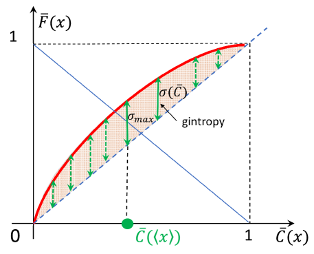
Figure 1: The cumulative number of citations, $\overline{F}$, plotted against the the cumulative publication fraction of those cited at least $x$ times, $\overline{C}$, - known also as the Lorentz curve. This plot also reveals visually the Gintropy $\sigma$ and the Gini index $G$: $\sigma$ is the distance between the Lorentz curve and the diagonal, $G/2$ is the area between these lines.

3 Hirsch index scaling

3.1 General considerations

The Hirsch index (or simply the ”h” index) [2], promoted to use for evaluation of scientific popularity of individuals, journals and institutions, is defined as that number of publications for which at least the same amount of citations has been collected:

$$h\>=\>N(x\geq h)\>=\>N_{\mathrm{pub}}\,\overline{C}(h).$$ (10)

For a given PDF, $\rho(x)$, the Hirsch index $h$ is the solution of the above equation, which in most of the common cases is transcendental.

Some distributions are special. Whenever they reflect some underlying scaling property, we expect that the Hirsch index is also subject to some consequential scaling. The question is in what construction can one make such a scaling apparent. In this paper we aim at constructing a scaling between the Hirsch index, $h$, the total number of publications, $N_{pub}$, and citations to those publications, $N_{cit}$. Note that $\left\langle{x}\right\rangle=N_{cit}/N_{pub}$.

In risk analysis the typical cumulative function has a form

$$\overline{C}(x)=\mathrm{e}^{-H(x)}.$$ (11)

In such cases the PDF, $\rho(x)=-d\overline{C}/dx$, becomes

$$\rho(x)=H^{\prime}(x)\,\mathrm{e}^{-H(x)}.$$ (12)

Here $H(x)$ is called the cumulative risk, while its derivative, $H^{\prime}(x)$ the risk rate [29].

Quite often the PDF-s used to fit statistical data have two common parameters, reflecting a shift and a magnification of the independent variable. These two parameters can be connected to the mean value and to the variation. As a formula one uses (or guesses) a universal function taken at a linear form of the argument. Assuming

$$H(x)\>=\>f(ax+b)$$ (13)

with a parameterless function, normalization criteria are automatically fulfilled for the PDF. The parameters $a$ and $b$ can be related to the expectation value, $\left\langle{x}\right\rangle$, and the remaining problem will contain only one single parameter. One can always choose $f(x)$ in a way that $a>0$.

Using eq.(13), and its inverse,

$$x\>\equiv\>\frac{f^{-1}(H)-b}{a},$$ (14)

one determines the following universal value

$$\kappa(b)\>\equiv\>a\left\langle{x}\right\rangle+b\>=\>\int_{f(b)}^{\infty}f^{-1}(H)\mathrm{e}^{-H}\,dH.$$ (15)

The cumulative risk, and with that all other functions related to the PDF, are parameterized in terms of $b$ only, and are functions of $x/\left\langle{x}\right\rangle$. Therefore such a scaling property is quite general.

$$H(x)=f\left([\kappa(b)-b]\frac{x}{\left\langle{x}\right\rangle}+b\right).$$ (16)

In conclusion, a very important subclass of PDF-s shows the scaling

$$\rho(x)\>=\>\frac{1}{\left\langle{x}\right\rangle}\,p\left(\frac{x}{\langle{x}\rangle}\right).$$ (17)

In these cases the cumulative integrals $\overline{C}$ and $\overline{F}$, and therefore the gintropy, $\sigma\equiv\overline{F}-\overline{C}$, depend only on the ratio to the expected value, $x/\left\langle{x}\right\rangle$, and the parameter $b$. Therefore

$$\overline{C}_{b}(h)\>=\>c_{b}\left(\frac{h}{\langle{x}\rangle}\right).$$ (18)

Knowing that $\left\langle{x}\right\rangle=N_{cit}/N_{pub}$, the Hirsch index is a solution of the general expression using the cumulative fraction:

$$\frac{h}{N_{pub}}=\mathrm{e}^{-f\left([\kappa(b)-b]\frac{h}{N_{pub}}\frac{N_{pub}^{2}}{N_{cit}}+b\right)},$$ (19)

since

$$\frac{h}{\left\langle{x}\right\rangle}=\frac{h}{N_{pub}}\,\frac{N_{pub}^{2}}{N_{cit}}.$$ (20)

From here it follows that there is a scaling between $N_{cit}$, $N_{pub}$ and $h$, based on the universal function, $f$, the parameter $b$ and its special integral summarized in $\kappa(b)$:

$$\frac{\sqrt{N_{cit}}}{N_{pub}}\>=\>\sqrt{[\kappa(b)-b]\frac{h/N_{pub}}{f^{-1}[-\ln(h/N_{pub})]-b}}.$$ (21)

Further scaling relations for the h-index can be obtained in various ways. They are not independent from the above result. We derive that $h/\left\langle{x}\right\rangle$ satisfies a consistency relation

$$\frac{h}{\left\langle{x}\right\rangle}\>=\>\frac{N_{\mathrm{pub}}^{2}}{N_{\mathrm{cit}}}\,c_{b}\left(\frac{h}{\left\langle{x}\right\rangle}\right)$$ (22)

For a fixed $b$ value the solution for this ratio depends on the single parameter

$$\lambda\>=\>\frac{N_{\mathrm{pub}}^{2}}{N_{\mathrm{cit}}}.$$ (23)

We note that $\lambda\left\langle{x}\right\rangle=N_{\mathrm{pub}}$, due to $\left\langle{x}\right\rangle=N_{\mathrm{cit}}/N_{\mathrm{pub}}$ being the average number of citations for the investigated distribution. Comparing now the two forms of the relations for the Hirsch index, equations (19) and (22)

$$\frac{h}{\left\langle{x}\right\rangle}=\lambda c_{b}\left(\frac{h}{\left\langle{x}\right\rangle}\right),\qquad\frac{h}{N_{\mathrm{pub}}}=c_{b}\left(\lambda\frac{h}{N_{\mathrm{pub}}}\right),$$ (24)

one realizes that both $h/\left\langle{x}\right\rangle$ and $h/N_{\mathrm{pub}}$ are functions of the single parameter combination, $\lambda$.

Multiplying the above two scaling laws, yields the already known forms:

$$\frac{h^{2}}{N_{\mathrm{cit}}}\>=\>\lambda c_{b}\left(\frac{h}{\left\langle{x}\right\rangle}\right)^{2}\>=\>\frac{h}{\left\langle{x}\right\rangle}c_{b}\left(\frac{h}{\left\langle{x}\right\rangle}\right).$$ (25)

The result is that for a constant parameter $b$ the ratio, $h^{2}/N_{\mathrm{cit}}$ depends only on the ratio $h/\left\langle{x}\right\rangle$, just like the gintropy does. Since the gintropy has a maximal value, one can derive from that an inequality for the $h^{2}/N_{\mathrm{cit}}$ ratio, too. According to [3], for most data sets

$$\sqrt{N_{\mathrm{cit}}}\approx 2h$$ (26)

3.2 Scaling for the Pareto distribution

The scaling Tsallis-Pareto distribution [25] is a special case of the distributions satisfying the form implied in (16). The validity of this for the distribution of citations of individuals was proven in [22]. The probability density function writes as:

$$\rho(x)=a\,b\,(1+ax)^{-b-1}$$ (27)

The tail-cumulative integrals in the Pareto case are given by:

$$\overline{C}(x)\>=\>(1+ax)^{-b}$$ (28)

$$\overline{F}(x)\>=\>\frac{(1+a\,b\,x)}{a}\>(1+a\,x)^{-b}$$ (29)

while the gintropy is

$$\sigma(x)\>=\>ab\,x\,(1+ax)^{-b}.$$ (30)

The Gini index can be also computed for the Tsallis-Pareto distribution. A simple mathematics leads us to

$$G_{TP}=\frac{b}{2b-1},$$ (31)

which is seemingly a general rule for the PDF’s characterizing the distribution of citations.

For the Tsallis-Pareto distribution, the (25) scaling relation write as:

$$\frac{h^{2}}{N_{\mathrm{cit}}}\>=\>\>\frac{h}{\left\langle{x}\right\rangle}c_{b}\left(\frac{h}{\left\langle{x}\right\rangle}\right)=\>\>\frac{h}{\left\langle{x}\right\rangle}\overline{C}_{b}(h)$$ (32)

Noting that $1/\left\langle{x}\right\rangle=a(b-1)$, and taking into account (29) and (30) we get

$$\frac{h^{2}}{N_{\mathrm{cit}}}\>=\>\frac{b-1}{b}\,\sigma(h).$$ (33)

Now, it has been shown in [15] that the gintropy has a maximum, therefore

$$\frac{h^{2}}{N_{\mathrm{cit}}}\leq(1-1/b)\,\max({\sigma}).$$ (34)

What remains is to obtain the maximum value of gintropy for the scaling Tsallis-Pareto distribution. Taking into account that the gintropy reaches its maximum for $x=\left\langle{x}\right\rangle$, this leads to:

$$\max(\sigma)=\sigma(\langle x\rangle)=\frac{b}{b-1}\left(1+\frac{1}{b-1}\right)^{-b}.$$ (35)

Using equation (34) we conclude that:

$$\frac{h^{2}}{N_{\mathrm{cit}}}\leq\left(1+\frac{1}{b-1}\right)^{-b}.$$ (36)

From the definition of the h index the scaling between $N_{cit}$, $N_{pub}$ and $h$:

$$\frac{h}{N_{pub}}=\overline{C}(h)\>=\>\left(1+\frac{h\,N_{pub}}{(b-1)\,N_{cit}}\right)^{-b}$$ (37)

This leads the special form of the scaling suggested in equation (21) as being

$$\frac{\sqrt{N_{cit}}}{N_{pub}}=\sqrt{\frac{h/N_{pub}}{(b-1)\,\left[(h/N_{pub})^{-1/b}-1\right]}}$$ (38)

4 Test on google scholar data

According to our former study [22], citation distributions are similar to the distribution of Facebook shares and scales according to a common Tsallis-Pareto distribution, with $b=1.4$. We have argued that the reason for this is the existence of the preferential dynamics in citations and the exponential growth in the number of publications (Facebook posts). Here we pursue a numerical investigation on the relation between the Hirsch index ($h$), citation number ($N_{cit}$) and total publication number ($N_{pub}$) of individual scientists on a large sample size. We intend to validate also our hypothesis regarding the Tsallis-Pareto shape of the probability density for the citation distribution and to reconsider the universality of the scaling exponent $b$.

Data are collected using a crawler internet robot, mapping the Google Scholar website.

In collecting citations we have started form a strongly connected author (Prof. H.E. Stanley) and mapped recursively his coauthor network. In this manner we collected the relevant data for 44 360 researchers with $N_{cit}\geq 10000$ and $N_{pub}\geq 100$. These limits were imposed in order to have enough data for constructing the probability density function. For each researcher, the Tsallis-Pareto fit was done automatically by covering the $b\in(1,8)$ values with a $\Delta b=0.025$ step. We searched for that $b$ value here for which we obtain the minima of the average relative difference squares:

$$s=\frac{1}{W}\sum_{i}^{W}\left(\frac{\log[\overline{C}^{exp}_{i}]-\log[\overline{C}^{theo}_{i}]}{\log[\overline{C}^{exp}_{i}]}\right)^{2},$$ (39)

Here $W$ denotes the number of experimental points used to quantify the distribution. We used the cumulative distribution function $\overline{C}(x)$ in order to have a smoother distribution of the experimental data. The logarithm was considered in order to fit accurately also the tail of the distribution, ensuring that all data points have the same order of magnitude.

On Figure 2 we first illustrate for a few randomly selected researchers with largely different citation numbers the validity of the Tsallis-Pareto PDF for their citations using $b$ exponents determined by our method. Here we collapsed the probability density functions for the citation distribution by considering the values relative to the mean and plotting $\rho(x/\langle x\rangle)$ as a function of $x/\langle x\rangle$.

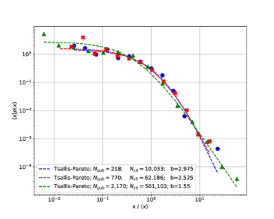
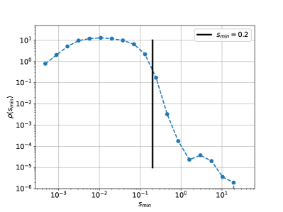
Figure 2: Validity of the Tsallis-Pareto form for the citations distribution. On the upper figure we illustrate the case of three researchers with very different $N_{cit}$ numbers. As the statistics gets better the Tsallis-Pareto fit also improves. In the figure from below we indicate the PDF for the distribution of the $s_{min}$ parameter, indicating the goodness of the Tsallis-Pareto fit for different researchers. The vertical line indicates the maximal limit accepted for our study.

The goodness of the fit can be characterized by the minimal $s$ value, denoted as $s_{min}$. The obtained distribution of the $s_{min}$ values is illustrated on log-log axes on the bottom Figure 2.

As we can observe from this Figure, the distribution has a long tail. Therefore we imposed an upper cutoff at $s_{min}=0.2$, and disregard in our further investigation those few cases where the Tsallis-Pareto fit is less reliable. Furthermore we disregarded also those cases where the best fit surpassed the imposed $b=8$ limit. From the initial $44360$ studied researchers we remained with $43656$ records.

The distribution of the fitted $b$ values for these researchers are given in Figure 5 where we have used again log-log axes. This distribution has a sharp peak around $b_{max}=1.32$ and indicates $\langle b\rangle=1.58$. The interval between the maximum value and the average is in good agreement with the scaling index suggested in our previous hypothesis [22].

Using the data for the researchers which passed the filters we are ready now to study the validity of the scaling relations presented in the previous section.

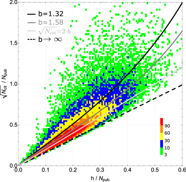
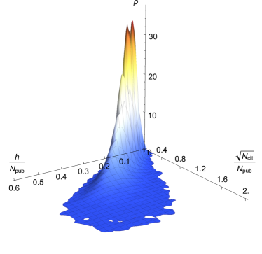
Figure 3: Validity and limits of the scaling relation between $h$, $N_{cit}$ and $N_{pub}$. In a 2D and 3D representation we illustrate the distribution of the points with coordinates ($\sqrt{N_{cit}}/N_{pub}$, $h/N_{pub}$). For the 2D representation the color-code given in the legend is used to indicate the density of the points. Different lines indicate the scaling for various $b$ Pareto exponents and the generally accepted $\sqrt{N_{cit}}=2h$ trend.

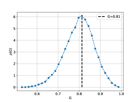
Figure 4: Distribution of the individualized Gini coefficient values for the studied researchers

Let us check first the scaling between $N_{cit}$, $N_{pub}$ and $h$, as indicated in eq. (38). In order to illustrate this scaling we plot $\sqrt{N_{cit}}/N_{pub}$ as a function of $h/N_{pub}$ for all the $43656$ records. On Figure 3 we indicate the density of these points by two methods. In the top Figure we use a 2D density plot, and in the bottom Figure we consider a 3D smoothed histogram representation. From the density plot representation it is clear that for small $h/N_{pub}$ values $\sqrt{N_{cit}}\propto h$, confirming the validity of the scaling expressed by eq. 26. The previously proposed scaling [3], $\sqrt{N_{cit}}=2h$ works perfectly for the bulk of our results. This figure also shows that the limits derived from the maximal values of Gintropy are applicable whenever we consider the $b=\infty$ limit. From here it a generally valid scaling follows, giving an interesting limit for the minimal number of citations for a given $h$ value.

$$\sqrt{N_{cit}}\geq h\lim_{b\rightarrow\infty}(1-1/b)^{-b/2}=h\sqrt{e}$$ (40)

This condition, $N_{cit}\geq eh^{2}$, is indeed much stronger than the obvious $N_{cit}\geq h^{2}$, and weaker than the previously proposed $N_{cit}=4h^{2}$, the latter works only for the main trend. The 3D plot (Figure 3b) indicates more convincingly that the spread of the data from the main trend is actually narrow.

As we have mentioned previously, the Tsallis-Pareto type distribution implies that the Gini coefficient satisfies: $G>1/2$. For all the selected researchers’ publications we have computed the individualized Gini index for the received citations. As expected, we find a wide distribution that peaks at $G=0.81$, corresponding to $b\approx 1.3$, indicating a large diversity for the citation numbers. The probability density function illustrated in Figure 4 presents a quite broad distribution, and we find our initial lower bound $G=1/2$ valid.

5 Discussion and Conclusions

The dimensionality of scientific performance has not only theoretical interest. The collection and analysis of scientific indicators is costly and complex. Reduction of the needed indicators attracted attention from scientometric research (see for example [5] and its bibliography). There are two approaches, the statistical one and the modelling one (cf. again [5, 4]). Here we followed the former approach with particular attention to the incorporation of the Hirsch index into the collection of indicators. The difficulty hides in the fact that the definition of the Hirsch index boils down to a functional equation which can not be solved explicitly. There are several studies which use parametric assumptions in order to find a good approximation for the Hirsch index. Among others the Pareto distribution by Glanzel in [6], geometric distribution by Bertoli-Barsotti & Lando [7], and the Weibull distribution used by [10] (see also the review [11] ). A numerical calculation of the transcendental equation for H conform (10) and (12) is given in [8].

Our first aim was to obtain a general non-parametric scaling relation for the h-index. In order to do so and to enjoy the formal analogy and nice properties of the gintropy and the survival description of the citation distribution, first we briefly recalled the Gini index and gintropy. Then the very general but implicit scaling of the h-index was derived with the aid of the gintropy formalism (21). Then we used the assumption that citations follow the Tsallis-Pareto distribution to obtain a more explicit expression. Selection of the location parameter and check of the validity of the arguments was done on Google Scholar data. In addition to the derivation of the scaling of the Hirsch index a new, sharper upper bound is now given for the h-index (40).

The universal citation pattern, unveiled in our previous studies [21, 22], is confirmed here by a statistically elaborated study on data collected from Google Scholar. Without limiting the studied research field in our statistical analyses, we find that the fitted Pareto exponents are distributed close to the previously proposed $b=1.4$ value (maximum at $b_{max}=1.32$ and mean at $\langle b\rangle=1.58$), but also show a heavy tail (Figure 5).

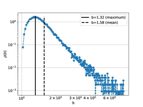
Figure 5: Distribution of the fitted $b$ values for the $43656$ researchers that passed the imposed filters.

This finding, suggested that the individualized Gini index, calculated for the citations of the publications of individual authors, should satisfy $G>1/2$. It is indeed in agreement with the data observed in Google Scholar. As a surprise we have learned, however, that the distribution of these individualized $G$ values considered for all the considered authors resembles a normal distribution that peaks a very high value, $G_{max}\approx 0.81$. This suggests a pronounce inequality among the number of citations that researchers receive for their publications. Furthermore, the Pareto-Tsallis type form for the distribution of citations of articles authored by researchers leads to several interesting connections and limits, concerning the total number of publications, the total number of citations and the h-index. The relation (38) derived from the Paretian shape of the distribution function is in agreement with data collected from Google Scholar. One concludes from the 3D representation of the data in Figure 3 showing a very sharp distribution of the data points, that such a scaling should indeed be valid. It is surprising, however, that inspecting Figure 3 one concludes that the previously proposed scaling [3] $\sqrt{N_{cit}}=2h$ follows more the peak of this distribution than the results obtained with $b_{max}$ or $\langle b\rangle$. The gintropy, as a novel inequality measure introduced recently [15], proved to be helpful in finding a proper limit for $h$ as a function of $N_{cit}$. The bound obtained by that argumentation, $N_{cit}\geq e\,h^{2}$, is nicely confirmed by the used Google Scholar data.

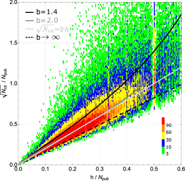
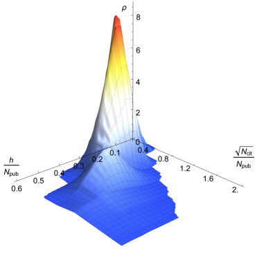
Figure 6: Distribution of the points with coordinates ($\sqrt{N_{cit}}/N_{pub}$, $h/N_{pub}$) in 2D and 3D representations considering the limits $N_{pub}\geq 10$ and $N_{cit}\geq 100$. To be compared with Figure 3

Finally, one should keep in mind that our statistical analyses are performed only on researchers with high productivity ($N_{pub}\geq 100$) and large number of citations ($N_{cit}\geq 10000$). Our starting hypothesis was already based on the fact that the distribution function for the citations can be described with a Tsallis-Pareto form. For understanding the applicability limits of our results it worth considering their generalization for researchers that have much less productivity and impact. Considering the limits $N_{pub}\geq 10$ and $N_{cit}\geq 100$, and keeping by this in the statistics more than 96% of the researchers mapped recursively with our crawler, the results corresponding to Figure 3 are presented now in Figure 6. The extended statistics suggests that the distribution of the points ($\sqrt{N_{cit}}/N_{pub}$, $h/N_{pub}$) are more spread, however the scaling $\sqrt{N_{cit}}=2\,h$ still follows the main trend. The limit $\sqrt{N_{cit}}\geq\sqrt{e}\,h$ is less evident, and 4.31% of the records violates it. This has to be compared with the case of largely cited researchers $N_{pub}\geq 100$ and $N_{cit}\geq 10000$, where only 0.16% of the researcher violates this limit. All these results confirm our initial working hypothesis according to which the proposed limits and scaling are based on the Pareto type distribution of citations, and are derived assuming that one can construct such a distribution function. Therefore one should be carefully with these results for the majority of those researchers that have a minor number of publications and citations.

Definitely, one may consider to perform even more proper data analyses by using scientifically more solid databases, like Web of Science or Scopus, however such studies should be more sophisticated in order to overcome the restrictive user policy of these databases. This is the main reason we have used here the freely available, although possibly less rigorous Google Scholar data.

Acknowledgements

This research was supported by UEFSCDI, under the contract PN-III-P4-ID-PCE-2020-0647.
T.S.B. thanks NKFIH for supporting research in the framework of the Hungarian National Laboratory Program under 2022-2.1.1-NL-2022-00002, which - among other indicators - requires to enhance citation and productivity in terms of publications. The work of M.J. was supported by the Collegium Talentum Programme of Hungary.

Competing interest

The authors declare no competing interest.

Author contributions

Conceptualization by TSB and ZN. Analysis by TSB and AT. Data mining and processing MJ and ZN. TSB, ZN and AT contributed in an equal manner to the first draft of the manuscript.

References

- [1] A. Schubert, & W. Glänzel, A dynamic look at a class of skew distributions. A model with scientometric applications. Scientometrics 6, 149-167 (1984).
- [2] J.E. Hirsch, An index to quantify an individual’s scientific output. PNAS 102, 16569-16572 (2005).
- [3] W. Glänzel, On the h-index - A mathematical approach to a new measure of publication activity and citation impact. Scientometrics 67, 315-321 (2006).
- [4] G. Siudem, B. Żogała-Siudem, A. Cena and M. Gagolewski, Three dimensions of scientific impact. PNAS 117, 13896-13900 (2020).
- [5] G. Prathap, Letter to the editor: comments on the paper of Gagolewski et al.: Ockham’s index of citation impact, Scientometrics 127, 6051-6054 (2022).
- [6] W. Glänzel, On some new bibliometric applications of statistics related to the h-index. Scientometrics 77, 187-196 (2008).
- [7] L. Bertoli-Barsotti, and T. Lando, On a formula for the h-index. Journal of Informetrics 9, 762-776 (2015).
- [8] L. Bertoli-Barsotti, and T. Lando, A theoretical model of the relationship between the h-index and other simple citation indicators. Scientometrics 111, 1415-1448 (2017).
- [9] L. Bertoli-Barsotti, and T. Lando, How mean rank and mean size may determine the generalised Lorenz curve: With application to citation analysis. Journal of Informetrics 13, 387-396 (2019).
- [10] L. Bertoli-Barsotti, and T. Lando, The h-index as an almost-exact function of some basic statistics. Scientometrics 113, 1209–1228 (2017).
- [11] L. Egghe, and R. Rousseau, The h-index formalism. Scientometrics 126, 6137-6145 (2021).
- [12] M. Gagolewski, B. Żogała-Siudem, G. Siudem, and A. Cena, Ockham’s index of citation impact. Scientometrics 127, 2829-2845 (2022).
- [13] A.L. Barabási and R. Albert, Emergence of scaling in random networks. Science 286, 509-512 (1999).
- [14] C. Gini, Sulla misura della concentrazione e della variabilità dei caratteri. Atti del Reale Istituto Veneto di Scienze, (Lettere ed Arti. A.A., 1914), pp. 1203-1248.
- [15] T.S. Biró and Z. Néda, Gintropy: Gini Index Based Generalization of Entropy, Entropy 22, 879 (2020).
- [16] J. Mingers and L. Leydesdorff, A Review of Theory and Practice in Scientometrics. European Journal of Operational Research 246, 1-19 (2015).
- [17] S. Alonso and F.J. Cabrerizo and E. Herrera-Viedma and F. Herrera, h-Index: A review focused in its variants, computation and standardization for different scientific fields. Journal of Infometrics 3, 273-289 (2009).
- [18] A. Bihari, S. Tripathi and A. Deepak, A review on h-index and its alternative indices, Journal of Information Science 0, 0165551521101447 (2021).
- [19] L. Bornmann, R. Mutz and H.D. Daniel, Are there better indices for evaluation purposes than the h index? A comparison of nine different variants of the h index using data from biomedicine. Journal of the American Society for Information Science and Technology 59, 830-837 (2008).
- [20] A. M. C. Sengor, How scientometry is killing science. GSA today 24, 44-45 (2014).
- [21] K. Barcza and A. Telcs, Paretian publication patterns imply Paretian Hirsch Index. Scientometrics 81, 513 (2009).
- [22] Z. Néda, L. Varga, T.S. Biró, Science and Facebook: the same popularity law! PLOS ONE 12, 0179656 (2017).
- [23] M.O. Lorenz, Methods of measuring the concentration of wealth. Publ. Am. Stat. Assoc. 9, 209-219 (1905).
- [24] T.S. Biró, A. Telcs, M. Józsa and Z. Néda, f-Gintropy: an Entropic Distance Ranking based on the Gini Index. Entropy 24, 407 (2022).
-
[25]
https://en.wikipedia.org/wiki/Generalized
_Pareto_distribution - [26] W. Glänzel, A. Telcs, and A. Schubert, Characterization by truncated moments and its application to Pearson-type distributions. Zeitschrift für Wahrscheinlichkeitstheorie und verwandte Gebiete 66, 173-183 (1984).
- [27] A. Schubert, and W. Glänzel, A dynamic look at a class of skew distributions. A model with scientometric applications. Scientometrics 6, 149-167 (1984).
- [28] A. Telcs, W. Glänzel, and A. Schubert, Characterization and statistical test using truncated expectations for a class of skew distributions. Mathematical Social Sciences 10, 169-178 (1985).
- [29] https://en.wikipedia.org/wiki/Survival_analysis
- [30] C. Tsallis, Introduction to Nonextensive Statistical Mechanics, Approaching a Complex World. (Springer 2009), pp. 41.