Towards indirect assessment of surface anomalies on wind turbine rotor blades

Abstract

We present results from novel field, lab and computer studies, that pave the way towards non-invasive classification of localised surface defects on running wind turbine rotors using infrared thermography (IRT). In particular, we first parametrise the problem from a fluid dynamical point of view using the roughness Reynolds number ($Re_{k}$) and demonstrate how the parameter regime relevant for modern wind turbines translate to parameter values that are currently feasible in typical wind tunnel and computer experiments. Second, we discuss preparatory wind tunnel and field measurements, that demonstrate a promising degree of sensitivity of the recorded IRT data w. r. t. the key control parameter ($Re_{k}$), which is a minimum requirement for the proposed classification technique to work. Third, we introduce and validate a local domain ansatz for future computer experiments, that enables well-resolved Navier–Stokes simulations for the target parameter regime at reasonable computational costs.

1 Background and motivation

With $132\text{\,}\frac{\mathrm{TW}\text{\,}\mathrm{h}}{}$ electricity fed into the grid in 2020, wind power has become Germany’s leading source of energy ($27\text{\,}\frac{\mathrm{\char 37\relax}}{}$) outperforming any fossil source [1]. However, cost reduction is indispensable to further strengthen the competitiveness of sustainable energy production beyond initial stages of massive subsidisation and political control. Rotor blade inspection of ageing wind turbines, for example, is elaborate and time-consuming and thus offers high potential to further reduce energy production costs through more efficient maintenance procedures [2, 3].

Health monitoring

of wind turbine blades usually employs visual inspection (from the ground or using drones and climbers), in order to assess damage and contamination level of the rotor blade’s surface (Fig. 1a–c).

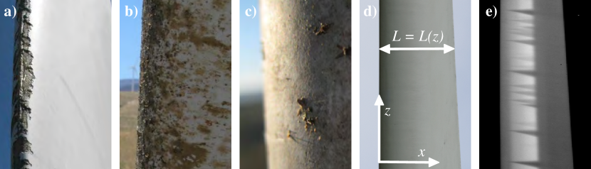
Figure 1: Problem description. a–c): Wind turbine rotor blades with typical surface defects as they occur during operation [4]. a): Heavy erosion of the blade’s leading edge due to impact (e. g., sand, rain, hail). b, c): Distributed and localised contamination with insect debris. d): Operating wind turbine in our preliminary field measurements in Thedinghausen. The blade suffers from naturally occurring surface anomalies, that are not visible from the ground ($>$100\text{\,}\frac{\mathrm{m}}{}$$). The streamwise direction is approximately in $x$-direction and the blade’s chord length ($L(z)\approx$5\text{\,}\frac{\mathrm{m}}{}$$) varies from root to tip. e): Thermographic image of the same blade (as in d), showing regions with higher (light) and lower (dark) surface temperature (black is blue sky compensation). Low temperature wedges indicate locally turbulent flow in the downstream wake of small localised surface anomalies in contrast to the otherwise laminar flow (high temperature).

These methods require a shutdown of the turbine and/or suffer from poor spatial resolution [5, 6]. Common alternatives (e. g. strain-gauges, optical and acoustical sensors) require elaborate instrumentation and suffer from costly recertification [2]. Additionally, some of these techniques heavily impair the aerodynamic performance of the rotor blades. More advanced techniques (e. g. ultrasonic, radiographic and electromagnetic testing) are sometimes used in well-controlled lab environments, but are essentially impossible to transfer to running wind turbines in the field.

Infrared thermography (IRT)

is an established diagnostic tool for indirect flow visualisation in aerofoil boundary layers [7], that overcomes the aforementioned drawbacks. It is based on the fact, that the convective heat flux between the fluid and the surface strongly depends on the local flow state (e. g. laminar or turbulent). For a given temperature difference between the incoming fluid and the aerofoil, flow state dependent spatial temperature gradients develop on the surface. This gradients can be measured by detecting the temperature dependent radiation from the surface with an infrared camera. For example, IRT has been used in well-controlled wind tunnel environments to detect laminar-turbulent transition and flow separation [8, 9, 10]. In these type of studies, the aerofoils are actively heated with $\mathcal{O}\!\left(${10}^{3}$\right)$\frac{\mathrm{W}}{{\mathrm{m}}^{2}}$$, to increase the convective heat flux density and thereby improving the thermal contrast (TC) between regions of different flow states. In contrast, applying IRT to operating wind turbines in the field is much more challenging because of several reasons [9]. First, active rotor blade heating is undesired. This heavily limits the maximum achievable TC, which now depends on local weather conditions and absorbed solar irradiation (i. e. $\mathcal{O}\!\left(${10}^{2}$\right)$\frac{\mathrm{W}}{{\mathrm{m}}^{2}}$$ during clear sky). Second, measuring from remote ground locations ($>$100\text{\,}\frac{\mathrm{m}}{}$$) causes large transmission losses and low contrast to noise ratios (CNR). Third, the camera exposure time must not exceed $\mathcal{O}\!\left(${10}^{-4}$\right)$\frac{\mathrm{s}}{}$$, in order to prevent blur due to rotor blade motion. Despite these constraints, IRT has been recently used to successfully detect premature laminar-turbulent flow transition due to surface anomalies in operating wind turbines [11, 12, 13, 14]. These achievements open new avenues to monitor damage and contamination level of wind turbine blades (Fig. 1a–c) via IRT of the blade’s surface (Fig. 1e) without shutting the turbine down for inspection nor modifying the rotor with additional sensors. For the application, however, it is not sufficient to simply detect the presence of an anomaly via IRT. Instead, it would be necessary to additionally infer exact position, size and shape of geometrical defects in order to enable remote classification of the surface anomaly; e. g. distinguish between erosion and deposition (Fig. 1a,b) or distinguish between different levels of contamination (Fig. 1b,c). This poses many methodological challenges and it is currently unclear, to what extent such a classification can be inferred faithfully from IRT images and whether physically informed modelling approaches might improve this endeavour.

Here we present

results from our preliminary studies paving the way towards indirect assessment of surface anomalies on running wind turbine rotor blades. In §2, we briefly summarise the state of the art in early laminar-turbulent transition in flat plate (Blasius) boundary layers and establish terminology necessary for the rest of the paper. In §3, we introduce a parametrisation of our problem in terms of the roughness Reynolds number ($Re_{k}$), which is commonly used to characterise roughness induced transition in Blasius boundary layers. In §4, we discuss new results from our wind tunnel and field measurements, that demonstrate a promising degree of sensitivity of the recorded IRT data with respect to $Re_{k}$. In §5, we introduce and validate a local domain ansatz for future computer simulations, that enables well-resolved 3d DNS for the target parameter regime at reasonable computational costs. In §6, we briefly propose future directions.

2 Turbulence transition in Blasius’ boundary layer flow

Probably the best understood example of boundary layer (BL) transition is a flat plate BL flow. In this canonical benchmark system, the streamwise velocity profile, $u_{x}=u_{x}(x,y)$, and thus the thickness of the BL, $\delta_{99}(x)$, are both very well described by the self-similar Blasius solution [e. g. 15]. The Blasius profile only depends on the wall-normal coordinate ($y$) and can be re-scaled for arbitrary streamwise locations ($x>0$) just by fixing the Reynolds number, $Re=\nicefrac{{x\,u_{\infty}}}{{\nu_{\infty}}}$, where $u_{\infty}$ and $\nu_{\infty}$ are the velocity and the viscosity of the fluid in the far field.

The Blasius BL becomes linearly unstable at $Re=\mathcal{O}\!\left(10^{5}\right)$. In experiments, however, this instability is bypassed and laminar-turbulent transition can occur at lower $Re$ due to finite-amplitude perturbations, which are usually present in the free-stream [16]. Especially relevant to our present work is the transition due to single (isolated) geometric perturbation elements on the plates surface, which perturb the velocity profile locally. Following a number of studies chiefly employing flow visualisations [17, 18], Klebanoff et al. [19] provided an in depth, quantitative analysis of the transition to turbulence caused by a semisphere glued to a flat plate’s surface. They showed that the key parameter governing the transition is the roughness Reynolds number, $Re_{k}=\nicefrac{{u_{k}\,k}}{{\nu_{\infty}}}$, where $k$ is the height of the roughness element (e. g. radius of the semisphere) and $u_{k}=u_{x}(x=x_{k},y=k)$ is the undisturbed streamwise velocity component at that height ($y=k$) and streamwise location ($x=x_{k}$). They placed semispheres with different $k$ at several $x_{k}$ and found a critical Reynolds number of $Re_{k}\approx$325$$, that is independent of $x_{k}$. They also studied a cylinder of unit aspect ratio ($\Gamma_{k}=\nicefrac{{k}}{{d}}=1$, where $d$ is the cylinders diameter) and found a critical Reynolds number of $Re_{k}\approx$450$$, which was lower than in most previous studies [18]. Since then, many experimental [20, 15, 21] and numerical [22, 23, 24, 25, 26] studies have been carried out, and it has been repeatedly highlighted that $Re_{k}$ is the main parameter governing transition, albeit the geometry of the element (including $\Gamma_{k}$) plays an important role as well. For the specific case of cylinders, Puckert & Rist [15] demonstrated a changeover from purely convective to global instability for transcritical $Re_{k}$ and an additional competition between varicose and sinuous instabilities, when the element is especially thin (i. e. large $\Gamma_{k}$). This indicates that the perturbation element solely acts as an amplifier in the subcritical regime (leading to symmetrical wake structures) and, additionally, as a wavemaker in the supercritical regime (leading to wake vortex shedding). We expect, that already these subtle differences, for example, will be distinguishable in the instantaneous wall-shear stress and thus in the plate’s surface temperature distribution as well, assuming a unit Prandtl number and Reynolds’ analogy to hold.

For wind turbines, however, we expect the curvature of the blade’s surface to play an important role for this specific transition scenario. First, because the curved geometry results in streamwise pressure gradients and velocity profiles that can deviate notably from the Blasius solution. Second, because the velocity profile is not self-similar, implying that a particular $Re_{k}$ can result from different combinations of $(x_{k},k)$, as discussed in §3. It is currently unclear to what extent these conditions change the underlying mechanisms (compared to Blasius’ scenario) and whether these changes might help or hinder our endeavour.

3 Relevant parameter space ($Re$-$Re_{k}$)

Modern wind turbines in the multi-megawatt class operate at Reynolds numbers up to $Re=${10}^{7}$$, where $x$ is taken to be $L$ (i. e. the local chord length of the rotor blade), and $u_{\infty}$ is taken to be the relative wind speed at a particular radial location ($z$) of the rotating blade (Fig. 1e) [27]. Modern wind turbines also employ rather thick rotor blade profiles (Fig. 2a) [28], so that even for large angle of attack ($\alpha$), the most prone location for surface anomalies due to foreign impact remains the vicinity of the blade’s leading edge ($\nicefrac{{x}}{{L}}\lesssim$0.2$$). In this region, the BL is typically laminar, since natural transition in wind turbine rotor blades usually occurs later ($\nicefrac{{x}}{{L}}\gtrsim$0.3$$). Now, we here consider generic geometric perturbation elements with a characteristic size ranging from $k=\mathcal{O}\!\left(10^{-5}\right)$\frac{\mathrm{m}}{}$$ (reflecting e. g. small sand grain) up to $k=\mathcal{O}\!\left(10^{-2}\right)$\frac{\mathrm{m}}{}$$ (reflecting e. g. insect debris) in order to model highly localised deposition on operating wind turbine rotor blades (Fig. 1c). Note, that more severe (distributed) contamination (Fig. 1b) and surface ablations (Fig. 1a) will be considered elsewhere. Furthermore, we begin by making the crude assumption, that the laminar BL in this region can be approximated by Blasius’ solution. This allows us, for the first time, to roughly quantify the relevant range of $Re_{k}$ for our problem by estimating the a priori unknown $u_{k}$ from the given parameter values ($Re$, $x_{k}$, $k$) discussed above.

The results are summarised in figure 2c.

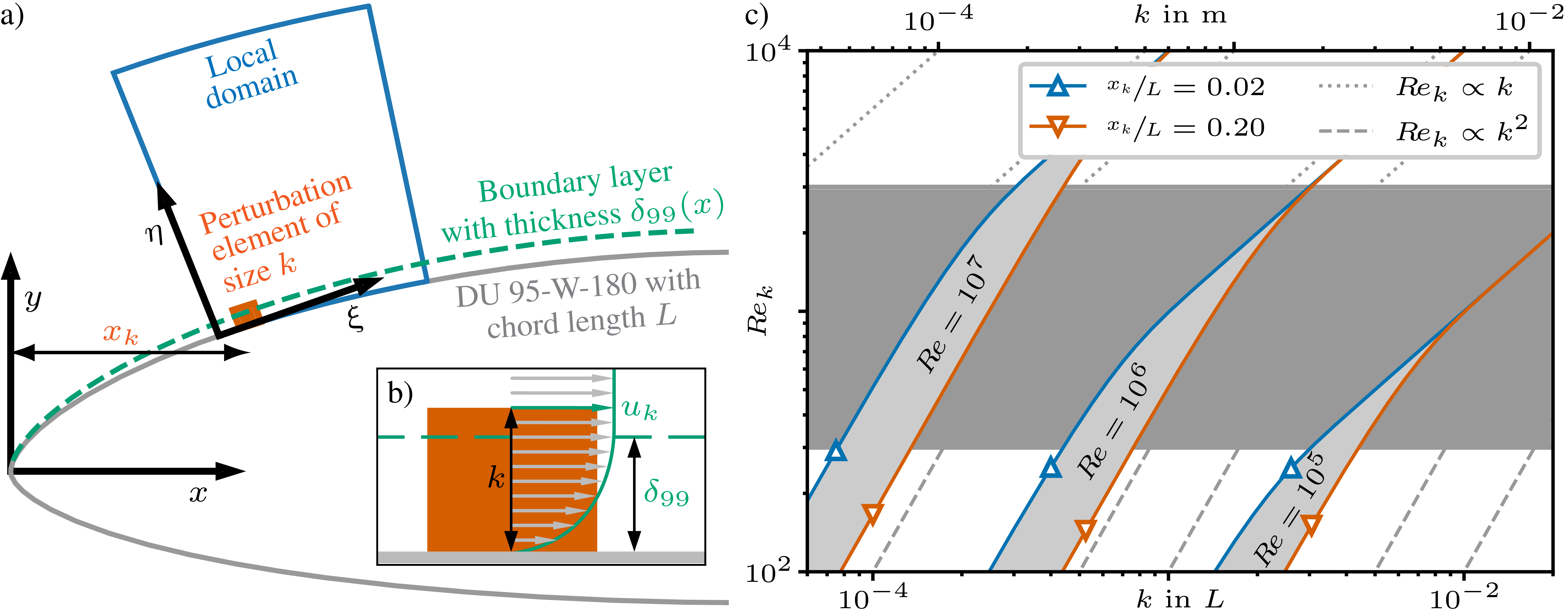
Figure 2: Parametrisation of the problem. a): Sketch of a typical wind turbine rotor blade profile (DU 95-W-180 [28]) with its leading edge at $(x=0,y=0)$ in the global coordinate system. A laminar boundary layer (broken line) is growing from its leading edge and a generic perturbation element is located at $\nicefrac{{x_{k}}}{{L}}\approx\nicefrac{{1}}{{10}}$. A local computational domain is placed around the perturbation element. b): Zoom of a. c): Relevant parameter space in terms of element size ($k$), position ($x_{k}$), chord ($Re$) and roughness ($Re_{k}$) Reynolds number, based on the crude assumption of a Blasius BL to estimate the local BL thickness, $\delta_{99}=\delta_{99}(x_{k})$, and the relevant velocity scale, $u_{k}=u_{k}(x_{k},k)$.

The dark grey region denotes the range of $Re_{k}$ realised in our preliminary wind tunnel campaign (at $Re=${10}^{5}$$, see §4), covering one order of magnitude from the sub-critical ($Re_{k}\approx$300$$) up to the fully turbulent ($Re_{k}\approx$3000$$) regime. Figure 2c also indicates, how these values translate to other situations; e. g., other combinations of $(x_{k},k)$ or higher $Re$. In this context, it is important to note, that for $k\ll\delta_{99}$ (i. e. element fully embedded in the linear part of the Blasius BL), $Re_{k}$ scales quadratic with $k$ for a given location ($x_{k}$), whereas for $k\gg\delta_{99}$ (i. e. element penetrates the flow outside the Blasius BL, as in fig. 2b), $Re_{k}$ scales only linear with $k$ and is thus basically independent of $x_{k}$. Where exactly this transition from the quadratic to the linear scaling takes place, depends on $Re$. In any case, relevant locations for generic perturbation elements would be $$0.02$<\nicefrac{{x_{k}}}{{L}}<$0.2$$, according to the discussion above. For a thick rotor blade profile (in contrast to the crude Blasius assumption here), the scaling in this two regimes will not be exactly quadratic and linear, due to curvature effects, but we expect the general behaviour to be qualitatively similar.

4 Infrared thermography (IRT)

We have performed preparatory IRT measurements on a running $1.5\text{\,}\frac{\mathrm{MW}}{}$-wind turbine in Thedinghausen, Germany, and on a down-scaled wind tunnel model using the Deutsche WindGuard facilities near Bremerhaven. Our results show, that it is feasible to distinguish between different localised perturbation elements in terms of their size ($k$) and location ($x_{k}$) by means of an IRT image of the blades’ surface temperature.

Already our field measurement at $Re=\mathcal{O}\!\left(${10}^{6}$\right)$ demonstrates a very promising degree of sensitivity of the IRT method w. r. t. different perturbations in the vicinity of the blade’s leading edge (Fig. 1e). Note, that here natural perturbations on the rotor blade’s surface (as they occur during operation) generate a variety of distinguishable thermal wake patterns in the IRT image. In particular, the different shades of dark grey wedges indicate regions of different temperatures at different locations on the blade’s surface that are presumably generated by surface anomalies of different size and location.

Our wind tunnel measurements at $Re=\mathcal{O}\!\left(${10}^{5}$\right)$ are a first successful effort to better quantify the underlying relationships between surface anomalies (cause) and their footprint in the surface temperature (effect). Here, we equipped the suction side of a typical rotor blade profile (DU 97-W-250 [28], $L=$30\text{\,}\frac{\mathrm{cm}}{}$$, $\alpha=$2\text{\,}\frac{\mathrm{\SIUnitSymbolDegree}}{}$$) with ten cylindrical perturbation elements of varying size ($k\in[$0.5$,$1.6$]$\frac{\mathrm{mm}}{}$$, constant $\Gamma_{k}=$0.3$$) and repeated the IRT measurements for three different element locations ($\nicefrac{{x_{k}}}{{L}}\in\{$0.03$,$0.1$,$0.2$\}$). Our results are summarised in figure 3.

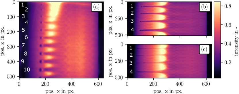
Figure 3: Sensitivity analysis in the wind tunnel. Shown are IRT images of the blade’s surface for fixed $(Re=${10}^{5}$,\alpha=$2\text{\,}\frac{\mathrm{\SIUnitSymbolDegree}}{}$)$ and varying $(Re_{k},x_{k})$, where higher/lower intensity reflects a warmer/cooler surface. The blade geometry is a DU 97-W-250 profile [28] with a constant chord length of $L=$30\text{\,}\frac{\mathrm{cm}}{}$$. a): Sensitivity of the thermogram for fixed $(\nicefrac{{x_{k}}}{{L}}=$0.2$)$ and varying $Re_{k}\in[$270$,$800$]$ in the transcritical regime, where we expect the onset of unsteady flow. The cylindrical perturbation elements are numbered from one to ten with increasing $Re_{k}$. b): Same as in a, but for $(\nicefrac{{x_{k}}}{{L}}=$0.1$)$. The four elements are numbered with increasing $Re_{k}\in[$800$,$3100$]$. c): Same as in b, but for $(\nicefrac{{x_{k}}}{{L}}=$0.03$)$.

Although $Re_{k}$ is the only control parameter in the flat plate transition scenario, it is apparent from fig. 2, that on an aerofoil, one particular $Re_{k}$ can be realised with different combinations of $(x_{k},k)$ for given free-stream conditions ($Re$). Thus, we first fix $\nicefrac{{x_{k}}}{{L}}=$0.2$$ to isolate the effect of varying $k$ (Fig. 3a). In this particular scenario, IRT is remarkably sensitive with respect to a varying $k$, which here corresponds to $Re_{k}\in[$270$,$800$]$. From element #3 on (i. e. $Re_{k}$ >$500$), a thermal signature is clearly visible in the downstream wake (Fig. 3a). This indicates that IRT is indeed capable of detecting weak transitional wakes at low trans-critical $Re_{k}$. If we now translate this first rough estimate of a minimum threshold for detectability ($Re_{k}\approx$500$$) to a real-word wind turbine scenario by making use of fig. 2b, we can conclude that our proposed measurement approach is suitable for detecting rotor blade defects as small as roughly $0.1\text{\,}\frac{\mathrm{mm}}{}$, with the exact threshold depending on both, $\nicefrac{{x_{k}}}{{L}}$ and $Re$. Additionally, the size of the wake pattern as well as its CNR w. r. t. the undisturbed (i. e. warmer) surrounding increase with $Re_{k}$ (Fig. 4a), thereby demonstrating a continuous sensitivity of our measurement approach.

Comparing figs. 3a, b, and c additionally demonstrates that the IRT method is clearly capable of distinguishing different $x_{k}$ in the entire range of relevant distances from the blade’s leading edge ($\nicefrac{{x_{k}}}{{L}}\in[$0.03$,$0.2$]$). However, for elements at $\nicefrac{{x_{k}}}{{L}}=$0.03$$, the wake pattern in the thermogram is less distinct when compared to the wake patterns originating from elements placed farther downstream (e. g. $\nicefrac{{x_{k}}}{{L}}=0.1$). In particular, the CNR of the thermal wake patterns increases twofold, when the perturbation elements are moved farther downstream (i. e. from $\nicefrac{{x_{k}}}{{L}}=0.03$ to $\nicefrac{{x_{k}}}{{L}}=0.1$). We conclude, that the position of a surface defect directly affects the detectability of its thermal wake pattern. Note, that for the four elements shown in figs. 3b and c, $Re_{k}\in[$800$,$3100$]$, which is considerably higher than the roughness Reynolds numbers shown in figure 3a.

5 Direct numerical simulations (DNS)

We have performed preparatory DNS of the incompressible Navier–Stokes equations using the spectral-element framework nektar++, which is purposely designed for high-fidelity flow simulations on unstructured grids in moderately complex domains. In order to enable well-resolved 3d DNS of laminar-turbulent transition in a rotor blade boundary layer with geometric perturbation elements at reasonable computational costs, we introduce and validate a local domain ansatz in massively reduced computational domains. We stress, that otherwise an extensive variation study of the relevant control parameters would be prohibitively expansive for the intended range of parameter values ($Re>${10}^{5}$$, $Re_{k}\gg$300$$).

The general idea of our local ansatz (Fig. 2a) goes as follows. First, we perform a 2d simulation of a typical wind turbine rotor blade (DU 95-W-180 [28]) in a large (global) computational domain without any perturbation element. Note, that we here use a sufficiently large domain (C-type, dimensions $$15$L\times$12$L$), in order to generate tailored inflow and pressure boundary conditions (BC) for much smaller local domains, that are located around the desired $x_{k}$. Recall, that the flow in the region of interest (i. e. $\nicefrac{{x}}{{L}}<$0.2$$) is always laminar, justifying our 2d approach. In a second step, we perform well-resolved 3d DNS in a local domain capturing only a small part of the curved rotor blade surface. In the future, this will allow us to include different isolated perturbation elements and, for the first time, investigate the transitional/turbulent flow in their downstream wake and the resulting local heat transfer between the fluid and the curved rotor blade surface in unprecedented detail.

Here we demonstrate the general viability of our ansatz (Fig. 4).

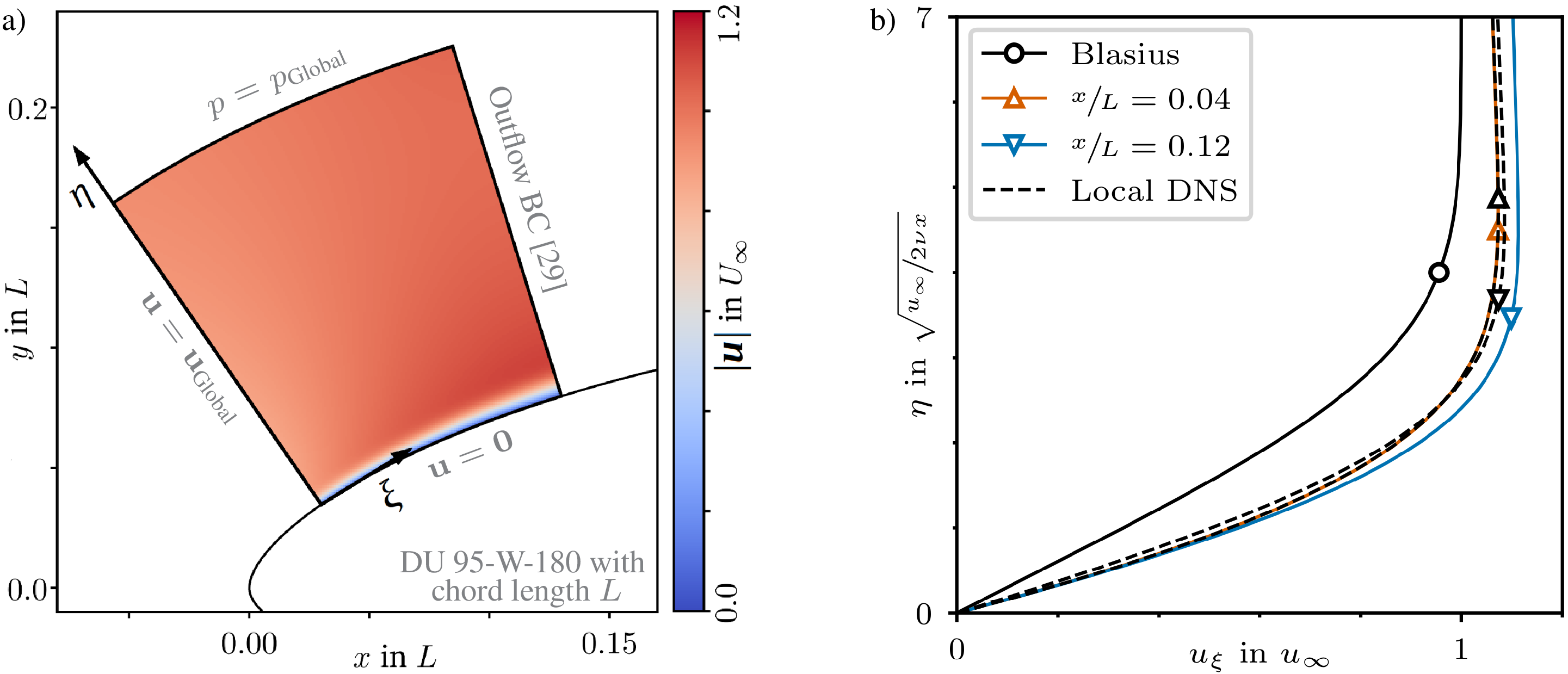
Figure 4: Local domain ansatz. a): Velocity field ($\lvert\boldsymbol{u}\rvert=\sqrt{u_{x}^{2}+u_{y}^{2}}$) generated in a local 2d simulation ($Re=${10}^{4}$$, domain at $$0.03$\leq\nicefrac{{x}}{{L}}\leq$0.13$$) of a clean rotor blade (DU 95-W-180 [28], $\alpha=$2\text{\,}\frac{\mathrm{\SIUnitSymbolDegree}}{}$$, w/o perturbation) using Dirichlet BC for $\boldsymbol{u}$ and $p$ as indicated and a robust outflow BC [29] at the right. b): Comparison of the velocity profile, $u_{\xi}(\eta)$, in the boundary layer at two different streamwise locations, $\nicefrac{{x}}{{L}}$, as predicted in local (broken lines) and global (full lines) DNS. The Blasius solution is given as reference.

For example, fig. 4b compares velocity profiles from a global and a local DNS run (here both 2d, $Re=${10}^{4}$$) and shows two things. First, the velocity profiles in the rotor blade boundary layer are, as expected, substantially different from the Blasius solution. Second, the results obtained from local DNS runs agree very well with the global DNS results. In particular, close to the inflow BC of the local domain ($\nicefrac{{x}}{{L}}=$0.04$$, where later perturbation elements will be placed), the velocity profiles are identical (judged by the given line width of the plot). Close to the outflow BC of the local domain ($\nicefrac{{x}}{{L}}=$0.12$$), the BL profiles have slightly diverged ($||u_{\zeta,\text{local}}-u_{\zeta,\text{global}}||_{\infty}\leq${10}^{-2}$$), but still show very good qualitative agreement. Note, that these results represent a worst-case scenario, since the local domain starts very close to the blade’s leading edge, where surface curvature has the strongest effect. For local domains that are located farther downstream (e. g. starting at $\nicefrac{{x}}{{L}}=$0.1$$ in order to capture perturbation elements farther away from the leading edge), we find that the deviations between local and global DNS results are even smaller (not shown). Note, that we have tested and analysed many different combinations of BC for the local DNS ansatz. In all cases, we have used Dirichlet and Neumann BC for $u$ and $p$, respecticaly, at the inflow (left) and the blades surface (bottom), where the values for the Dirichlet BC were extracted from the global run. The results presented in fig. 4, we obtained using pressure Dirichlet BC at the top and the robust outflow BC of Dong et al. [29] at the rigth. Other combinations of BC for the top/right boundaries yield very similar results with locally slighty better agreement, depending on the region of interest (i. e. either inside or outside the BL).

6 Perspective

Our preliminary studies show two things. First, IRT is sufficiently sensitive to distinguish between different size and location of highly localised perturbation elements in typical wind turbine rotor blade boundary layers. Second, the proposed local domain ansatz is feasible to approximate the boundary layer flow on a typical rotor blade profile sufficiently well, allowing for well resolved Navier–Stokes simulations of the underlying problem at reasonable computational costs.

Future works should aim at generating a comprehensive surface-state-flow-pattern catalogue and a deeper physical understanding of how surface irregularities in the vicinity of the blade’s leading edge (cause) affect the downstream surface temperature distribution (effect). Here, it is particularly interesting to clarify, how much information about the three-dimensional flow in the wake is actually contained in its two-dimensional surface temperature projection, since the inverse problem (effect to cause) is not bijective. To this end, extensive wind tunnel and computer experiments could be combined in order to systematically characterise the effect of different generic surface anomalies on early transition and the resulting (turbulent) wake in a rotor blade boundary layer and the resulting temperature footprint. Hopefully, this will lay the foundation for the development of a data-trained physics-informed model to reliably relate individual thermographic images to particular rotor blade conditions based on image recognition and machine learning techniques.

We gratefully acknowledge

resources and support provided by Nicolas Balaresque (Deutsche WindGuard) and the North German Supercomputing Alliance (HLRN).

References

- [1] Strom-Report. Germany’s Power Mix 2020 — Data, Charts & Key Findings (2021). URL https://strom-report.de/germany-power-generation-2020/
- [2] D. Li, S.C.M. Ho, G. Song, L. Ren, H. Li, Smart Materials and Structures 24(3) (2015)
- [3] F.P. García Márquez, A.M. Peco Chacón, Renewable Energy 161, 998 (2020)
- [4] R.S. Ehrmann, B. Wilcox, E.B. White, D.C. Maniaci, Effect of Surface Roughness on Wind Turbine Performance. Tech. Rep. 10, Sandia National Laboratories, Albuquerque (2017)
- [5] D.Y. Kim, H.B. Kim, W.S. Jung, S. Lim, J.H. Hwang, C.W. Park, in 44th International Symposium on Robotics (IEEE, 2013), pp. 1–5
- [6] M. Shafiee, Z. Zhou, L. Mei, F. Dinmohammadi, J. Karama, D. Flynn, Robotics 10(1), 1 (2021)
- [7] E. Gartenberg, A.S. Roberts, Journal of Aircraft 29(2), 161 (1992)
- [8] S. Montelpare, R. Ricci, International Journal of Thermal Sciences 43(3), 315 (2004)
- [9] C. Dollinger, M. Sorg, N. Balaresque, A. Fischer, Experimental Thermal and Fluid Science 97, 279 (2018)
- [10] C. Dollinger, N. Balaresque, N. Gaudern, D. Gleichauf, M. Sorg, A. Fischer, Renewable Energy 138, 709 (2019)
- [11] D. Traphan, I. Herraéz, P. Meinlschmidt, F. Schlüter, J. Peinke, G. Gülker, Wind Energy Science 3(2), 639 (2018)
- [12] T. Reichstein, A.P. Schaffarczyk, C. Dollinger, N. Balaresque, E. Schülein, C. Jauch, A. Fischer, Energies 12(11), 2102 (2019)
- [13] D. Gleichauf, M. Sorg, A. Fischer, Applied Sciences 10(18) (2020)
- [14] A.M. Parrey, D. Gleichauf, M. Sorg, A. Fischer, Applied Sciences 11(18), 8700 (2021)
- [15] D.K. Puckert, U. Rist, Journal of Fluid Mechanics 844, 878 (2018)
- [16] L. Brandt, P. Schlatter, D.S. Henningson, Journal of Fluid Mechanics 517, 167 (2004)
- [17] L. Klanfer, P.R. Owen, The effect of isolated roughness on boundary layer transition. Tech. rep., Royal Aircraft Establishment (1953)
- [18] A.M.O. Smith, D.W. Clutter, J. Aeros. Sciences 26(4), 229 (1959)
- [19] P.S. Klebanoff, W.G. Cleveland, K.D. Tidstrom, Journal of Fluid Mechanics 237(101), 101 (1992)
- [20] Q. Ye, F.F. Schrijer, F. Scarano, International Journal of Heat and Fluid Flow 61, 31 (2016)
- [21] Q. Ye, F.F. Schrijer, F. Scarano, Journal of Fluid Mechanics 837, 597 (2018)
- [22] J.A. Masad, V. Iyer, Physics of Fluids 6(1), 313 (1994)
- [23] J.H. Fransson, L. Brandt, A. Talamelli, C. Cossu, Physics of Fluids 17(5), 1 (2005)
- [24] J.C. Loiseau, J.C. Robinet, S. Cherubini, E. Leriche, Journal of Fluid Mechanics 760, 175 (2014)
- [25] D. De Grazia, D. Moxey, S.J. Sherwin, M.A. Kravtsova, A.I. Ruban, Physical Review Fluids 3(2), 1 (2018)
- [26] J. Casacuberta, K.J. Groot, Q. Ye, S. Hickel, Flow, Turb. Combustion 104(2-3), 533 (2020)
- [27] M. Ge, D. Tian, Y. Deng, Journal of Energy Engineering 142(1), 04014056 (2014)
- [28] W.A. Timmer, R.P.J.O.M. van Rooij, J. Solar Energy Engin. 125(4), 488 (2003)
- [29] S. Dong, G.E. Karniadakis, C. Chryssostomidis, Journal of Computational Physics 261, 83 (2014)