A practically efficient fixed-pivot selection algorithm and its extensible MATLAB suite

Abstract

Many statistical problems and applications require repeated computation of order statistics, such as the median, but most statistical and programming environments do not offer in their main distribution linear selection algorithms. We introduce one, formally equivalent to quickselect, which keeps the position of the pivot fixed. This makes the implementation simpler and much practical compared with the best known solutions. It also enables an “oracular” pivot position option that can reduce a lot the convergence time of certain statistical applications. We have extended the algorithm to weighted percentiles such as the weighted median, applicable to data associated with varying precision measurements, image filtering, descriptive statistics like the medcouple and for combining multiple predictors in boosting algorithms. We provide the new functions in MATLAB, C and R. We have packaged them in a broad MATLAB toolbox addressing robust statistical methods, many of which can be now optimised by means of efficient (weighted) selections.

Keywords— quickselect, order statistics, weighted percentiles, medcouple, robust methods, MATLAB, C, R

1 Introduction

The well-known selection problem consists in finding the $k$-th order statistic of an unsorted array of $n\geq k$ elements, assumed distinct and with all their permutations equally likely. It is thus defined on a totally ordered set $U$ as:

Input : An array $A=(a_{1}\ldots a_{n})$ and an integer $k$ such that $1\leq k\leq n$ and $a_{i}\in U$ for each $i=1,\ldots,n$.

Output : $a_{(k)}$, the $k$-th smallest element of $A$.

The index notation $(k)$ indicates the rank of the $k$ element of the array $A$, which is the index in the order statistics list $R_{k}(A)=\sum_{i=1}^{n}I_{[0,\infty)}(a_{k}-a_{i})$, being $I$ the indicator function. The rank $(k)$ can be associated to the statistical percentile $p_{k}$ by $(k)=\lceil\frac{p_{k}}{100}\cdot n\rceil$, where the ceiling function $\lceil\cdot\rceil$ gives the least integer greater than or equal to its argument. The median of $A$, say $\tilde{A}$, is a particular instance of the selection problem when $n$ is odd, that is: if $n=2m+1$ for an integer $m$ then $\tilde{A}=a_{(m+1)}=a_{(\frac{n+1}{2})}$. Otherwise, when $n=2m$, $\tilde{A}$ is the arithmetic mean of the two middle order statistics $a_{(m)}=a_{(\frac{n}{2})}$ and $a_{(m+1)}=a_{(\frac{n}{2}+1)}$.

The time-complexity $T(n)$ of selection algorithms is measured by counting the number of comparisons and exchanges between elements of $A$. The best partitioning-based methods - like the celebrated quickselect [Hoare’s Find, 31, 32] - take on average linear-time, but in the worst case $T(n)$ becomes quadratic. Solutions that theoretically behave linearly also in the worst case [10, 17] pose considerable implementation issues – and even take in practice more CPU time than the naive counterparts based on sorting [8] – while it is avowed that applications require more “useful practical algorithms” [53, p. 347]. This paper considers an algorithm of simple implementation that satisfies this functional requirement, and we therefore named it simpleselect.

The simplifications are procured thanks to an iterative fixed pivot position strategy that makes in-place array swaps around position $k$ (Section 2). Its efficiency is equivalent to that of quickselect (Section 3) and the chance of incurring in quadratic run-time is averted, as usual, by randomizing the initial array at a marginal cost of $\mathcal{O}(n)$ exchanges (we use backward shuffling [37, pp. 124-125], based on results by [21, pp. 26-27]). Thus, quickselect and simpleselect are equivalent “Las Vegas” algorithms: both produce same correct output, but while the former randomizes the pivot position at each execution step, the latter randomizes the initial array once.

The fixed pivot and resultant simplifications enable two useful extensions. The first consists in an “oracle” suggesting where the order statistic value can be found in $A$. Section 4 demonstrates its benefit in two renowned robust multivariate estimators. The second is the extension to weighted percentiles, discussed in Section 5.

In order to ease portability and usability, we have implemented simpleselect and its weighted form in MATLAB, C and R, which do not provide alternatives in their main distribution. Their filename is quickselectFS and quickselectFSw, to stress the equivalence with Hoare’s algorithm. We illustrate how to incorporate calls to the C function with an example in Python (Annex A.3). To facilitate the assessment of the functions in the different environments and under general simulation settings, we have also introduced a new MATLAB function that allows reproducing random numbers generated by R software with Mersenne Twister (Annex A.4).

Obviously, the practical benefit of the new functions can be appreciated only in combination of other general methods relying on repeated computation of order statistics and weighted percentiles. Therefore, we have packaged them in FSDA [47, 48], an extensive MATLAB library especially addressed to robust statistics, open to contributions through GitHub. For the same reason, we have enhanced the package with new efficient functions to compute the theoretical distribution of the number of comparisons in quickselect-like procedures [5] (Section A.2) and the medcouple [13] (Section 5.3), a robust skewness estimator that calls intensively the weighted median.

We ran simulations on an Intel CPU 2.9 GHz Quad-Core i7, equipped with 16 GB RAM. We developed under MATLAB release R2021b, but results are consistent in much older releases.

2 Simpleselect

2.1 Concepts

If the array $A$ is ordered fully, or partially till position $k$, clearly $a_{(k)}=a_{k}$. But (partially) sorting the array is more than what we need if only the element $a_{(k)}$ is of interest. Knuth [37, pp. 207–219] has magisterially assembled the historical roots and efforts spent to find solutions in $\mathcal{O}(n)$ time, relying on adaptations of quicksort [30, 18] in a divide and conquer partitioning approach consisting of:

1. A criterion to choose the position $s$ of an element $a_{s}\in A$ called pivot.

2. A procedure to rearrange the other elements of $A$ so that those in positions $1$ to $s-1$ will be smaller than those in positions $s+1$ to $n$.

Depending on the relative positions of the pivot and the desired order statistic, (1) and (2) are applied recursively or iteratively to one of the two parts of $A$:

• if $s>k$ the new target is the $k$-th element in the left side part;

• if $s<k$ the new target is the the $(k-s)$-th element in the right side part;

• if $s=k$ the element in position $s$ is the desired order statistic $a_{(k)}$.

In Hoare’s Find the pivot is chosen at random. More complex partition-based algorithms, such as the median of medians [10] and introselect [44], are conceptually identical, but differ for the criterion used to choose the pivot in a reasoned way – sometimes abstruse – in order to achieve linear worst-case.

In the following we show the practical advantages of the simpleselect strategy, which keeps the pivot in fixed position $k$ and iterates the swap of its value with numbers around it (right/left parts) until the pivot gets the correct value, rather than moving the pivot position (randomly or with another strategy) until it reaches the desired position $k$. The performance of this simplified iterative strategy remains aligned to the best known solutions. Abandoning recursion also ensures scalability to large arrays, as it avoids stack keeping issues common to most computing environments. We found a similar strategy, yet confined to the median computation, in https://rosettacode.org/wiki/Rosetta_Code. To the best of our knowledge, its properties have not been studied.

2.2 Permuting in-place

Finding $a_{(k)}$ requires a permutation $\left(\sigma(1),\ldots,\sigma(n)\right)$ of the elements of $A$ such that $a_{\sigma(1)},a_{\sigma(2)},\ldots,a_{\sigma(k-1)}\leq a_{\sigma(k)}$ or, equivalently, $a_{\sigma(k)}<$ $a_{\sigma(k+1)},a_{\sigma(k+2)},\ldots,a_{\sigma(n)}$. This is obtained with a sequence of swaps determined by the element $a_{k}$. Let us indicate with $A^{t}$ the status of the array at a given step $t\in\cal{N}$, with $a^{t}_{k}$ its element in position $k$, and with

$$A_{L_{k}}^{t}=\{a^{t}_{i}\in A^{t}\;|\;a^{t}_{i}\leq a^{t}_{k} \land\quad i<k\}$$

$$A_{R_{k}}^{t}=\{a^{t}_{i}\in A^{t}\;|\;a^{t}_{i}>a^{t}_{k} \land\quad i>k\}$$

the sets of left and right elements of $a^{t}_{k}$ that at step $t$ satisfy the desired ordering. The order statistic $a_{(k)}$ is found for some $t$ when $\big{|}A_{L_{k}}^{t}\big{|}=k-1$ or, equivalently, $\big{|}A_{R_{k}}^{t}\big{|}=n-k+1$. At step $t$ the set $A_{L_{k}}^{t}$ can be built with at most $k-1$ comparisons. Note that, for the symmetry of the problem, (i) we can avoid examining $A_{R(k)}^{t}$; (ii) there is no difference in solving for $k>\lceil\frac{n}{2}\rceil$ or $k<\lceil\frac{n}{2}\rceil$; (iii) finding $k=\lceil\frac{n}{2}\rceil$ is the most demanding case. We can now express the selection problem in algorithmic form:

Input : $A=(a_{1}\ldots a_{n})$ and $k$

while $\big{|}A_{L_{k}}^{t}\big{|}\neq k-1$ do

       Select element $a_{k}$ as pivot $a^{t}_{k}$ ;

       Build the set $A_{L_{k}}^{t}$, with a series of swaps relying on comparisons with $a^{t}_{k}$ ;

       Evaluate the cardinality of $A_{L_{k}}^{t}$;

      

end while

Output : $a_{k}$

The key parts of the algorithm can be recognized in the code listing (1), distilled from function quickselectFS.m. The code uses three variables to control the progression of $A_{L_{k}}^{t}$ and $A_{R_{k}}^{t}$: one is position and the others are two ‘sentinels’ left and right such that $\mbox{{left}}\leq\mbox{{position}}$ and $\mbox{{right}}>\mbox{{position}}$ at each iteration step $t$. Note that each change of position is associated to a swap operation. Note also that, for the symmetry of the problem, we could focus only on the left part of the array; this means that the loop terminates when $\mbox{{left}}=\mbox{{position}}+1=k+1$. A last remark is on the intense for cycle at line 13, which runs only until right-1: this is because $A(\mbox{{right}})$ receives the pivot element at line 10 and thus the if statement at line 14 is never true when $i=\mbox{{right}}$.

Listing 1: Code distilled from quickselectFS.m. Also available as R, C and C-mex files.

⬇

1ction [kE] = quickselectFS(A,k)

2% Finds the k-th order statistic using SimpleSelect

3left = 1;

4right = numel(A);

5position = -1;

6while (position$\sim$=k)

7 %% Part one: select element in position $k$ as pivot

8 pivot = A(k); %|

9 A(k) = A(right); %| Swap

10 A(right) = pivot; %|

11 position = left; % c2

12 %% Part two: build set $A_{L_k}^{t}$

13 for i=left:right-1

14 if(A(i)<pivot)

15 buffer = A(i); %|

16 A(i) = A(position); %| Swap

17 A(position) = buffer; %|

18 position = position+1; % c1

19 end

20 end

21 A(right) = A(position);

22 A(position) = pivot;

23 %% Part three: evaluate cardinality of $A_{L_k}^{t}$

24 if (position < k)

25 left = position + 1; % c2

26 else

27 right = position - 1;

28 end

29end

3 Counting comparisons

This section shows that simpleselect performs like quickselect and is therefore suitable to the applications discussed in Section 4. Abandoning recursion precludes the derivation of theoretical time bounds using recurrence equations. We therefore adopt a simple counting approach.

3.1 Worst case

We start counting the number of comparisons $c(n)$ in the worst case, occurring when at each cycle $t$ the set $A_{L_{k}}^{t}$ contains exactly $t-1$ elements. This happens when we look for the maximum ($k=n$) among elements in increasing order except the last containing the minimum ($a_{1}<a_{2}<\ldots<a_{n-1}$ and $a_{n}=a_{(1)}$). In this case (and the symmetric one for $k=1$), variable position is never modified inside the for cycle. Figure 1, produced with a function written to demonstrate the dynamic of simpleselect, illustrates the status at the first and forth while iteration of an array with this unfortunate order.

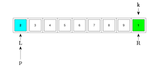
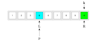
Figure 1: simpleselect in the worst case. Left panel, first while iteration: $|A_{L_{9}}^{1}|=0$. Right panel, forth while iteration: $|A_{L_{9}}^{4}|=3$. To reproduce, use ckselectFS_demo(A,k) with $A=[2,3,4,5,6,7,8,9,1]$ and $k=9$.

As comparisons are done at lines $6$, $14$ and $24$ of the code listing (1), we specify the count breakdown with $c(n)=c_{6}(n)+c_{14}(n)+c_{24}(n)$. Then we indicate with $(t,l,r,p)$ the status of variables left, right and position at step $t$. With this notation we have:

$$(t,l,r,p)=(1,1,n,1) \Rightarrow c(n)=1+(n-0)+1$$

$$(t,l,r,p)=(2,2,n,2) \Rightarrow c(n)=1+(n-1)+1$$

$$\vdots$$

$$(t,l,r,p)=(n,n,n,n) \Rightarrow c(n)=1+(n-(n-1))+1$$

Therefore, the worst number of comparisons is quadratic:

$$c(n)=2n+n^{2}-\sum_{i=0}^{n-1}i=2n+n^{2}-\frac{(n-1)n}{2}=\frac{n^{2}+5n}{2}.$$ (1)

Figure 2: simpleselect. Empirical number of comparisons $c(n)$ for finding the maximum in a uniformly generated sample. Left panel: $\max(c(n))$ and $\mbox{mean}(c(n))$ in $r$ replicates; the line fit on the mean case is $\hat{c}(n)=2\,n$. Right panel: empirical distribution of $c(n)/n$ for $n=1000$ (bar style) and $n=50$ (stairs style), with superimposed the Dickman distribution (translated by 1) obtained using FSDA function vervaatxdf with parameter $\beta=1$.

Note that $c_{6}(n)$ and $c_{24}(n)$ only involve index comparisons with short integers, which typically cost much less than a data comparison $c_{14}(n)$ on the array content. If we ignore them, equation (1) reduces to $c(n)=(n^{2}+n)/2$.

3.2 Average case

We can reason about how the linear complexity is achieved in practice with average case considerations, which the simplified code makes almost trivial. At the first execution of the while statement, a comparison is done at line 6 to check the exit condition, then one is done at line 24, and another $n$ are executed inside the for cycle of line 13-20. The exit condition set on position is approached:

• at line 18, where position is incremented by a step whenever $a_{i}<\mbox{{pivot}}$;

• at line 25, where left jumps to the cell after position and this makes also position to make a step ahead, being set to left at line 11.

If $A$ is a random sample of elements extracted from the same distribution, we expect $(n-1)/2$ increments of position in the initial scan of $A$ (see Annex A.1). Likewise, the increment of variable left at lines $25$ and $11$ - and similarly for variable right - which further reduces the distance to position, is done at most once. Then, at the second execution of the while statement the for cycle is expected to run on about (less than) $n/2$ array cells (actually, $(n-1)/2-1=(n-3)/2$). And so on for the subsequent steps:

$$\begin{array}[]{lcll}(t,l,r,p)=(1,1,n,1)&\Rightarrow&c(n)=1+n+1\\ (t,l,r,p)=(2,\cdot,n,\cdot)&\Rightarrow&c(n)=1+n/2+1\\ (t,l,r,p)=(3,\cdot,n,\cdot)&\Rightarrow&c(n)=1+n/4+1\\ &\vdots&\\ (t,l,r,p)=(\log_{2}n,n,n-1,n)&\Rightarrow&c(n)=1+n/2^{(log_{2}n-1)}+1\end{array}$$

The total therefore is:

$$c(n) =\displaystyle 2\log_{2}n+n\sum_{t=1}^{\log_{2}n}\frac{1}{2^{t-1}} = \;2\log_{2}n+n\sum_{i=0}^{\log_{2}n-1}\frac{1}{2^{i}}$$

$$=\displaystyle 2\log_{2}n+n+n\sum_{i=1}^{\log_{2}n-1}\frac{1}{2^{i}} = \;2\log_{2}n+n+n(1-\frac{1}{2^{\log_{2}n-1}})$$ (2)

$$=\displaystyle 2\log_{2}n+n+n(1-\frac{2}{2^{\log_{2}n}}) = \;2\log_{2}n+n+n(1-\frac{2}{n})$$

$$=\displaystyle 2\log_{2}n+2n-2 < \;2n+18\qquad\mbox{for}\;n<1000$$ (3)

where the partial sum of the first $\log_{2}n-1$ terms of the geometric series in (2) is computed with standard algebraic steps, and the final upper bound (3) reduces the logarithmic term to a constant that increases barely with $n$ compared to $2n$. Note that the conclusion is in line with the empirical results of Figure 2, which indeed bode for a $2n$ term, and with known asymptotic results based on the recurrent relations of recursive partitioning methods [as in 40, Theorem 1].

3.3 Number and empirical distribution of comparisons

The left panel of Figure 2 shows with symbol ‘$*$’ the progression of equation (1) and the actual number of comparisons required by simpleselect for finding in $r$ replicates the maximum in a set of $n$ integers extracted uniformly between 1 and (to avoid repetitions) $10000\,n$. For small sample sizes the two curves of the maximum follow the quadratic shape of equation (1), as the $r$ replicates are enough to fall in the worst possible scenario (extract the $n$ values in the above mentioned order). Then they start growing linearly, with an empirical worst-case of approximately $5\,n$ (the fit is for $r=100000$ and $n$ up to $1000$). Similarly, the third (dotted) line shows that on average $2\,n$ comparisons are sufficient to find the maximum.

We also checked the empirical distribution of $c(n)/n$: for sufficiently large $n$ it follows the Dickman distribution shown in the right panel of Figure 2, which is the limiting distribution for Hoare’s Find (see [34] and related works by [26, 27]). It is remarkable that the Dickman adaptation is rather good also for small sample sizes ($n=50$). Given the centrality of the Dickman distribution in this context, we provide functions for the computation of the pdf, cdf and the generation of random variates of the wider Vervaat class, following the works mentioned in Appendix A.2. These functions can be used to study partitioning algorithms different from Hoare’s Find, which can lead to other limiting results [39].

3.4 Run-time results

Our baseline for the run-time results is the internal (built-in) sort function – $SORT_{int}$ – which a typical MATLAB user would use because the standard distribution do not have functions dedicated to order statistics (prctile and median use sort). For assessing the actual performances of simpleselect, we consider two execution modes of our implementation: the just-in-time (jit) compilation where MATLAB directly analyses and translates the source code during a run (this is the standard execution modality of MATLAB, also available in R), and the mex-file mode where we compile a C-code instance of simpleselect into machine-code before any subsequent execution. The two instances, identified later with $SS_{jit}$ and $SS_{mex}$, are then compared with the classic implementation of quickselect of Numerical Recipies in C [46, Section 8.5] – $NURE_{mex}$ – and the introselect available in the C++ function nth_element – $NthEL_{mex}$ – both compiled as mex-file. The latter is also distributed as mex file by [38], but uses undocumented calls that may change and break in the future.

Input : $pdfName$, $nSet$, $kSet$, $r$

for n=nSet do

       for k=kSet do

             for i=1:r  do

                   $A_{n}\leftarrow$ $n$-sample from distribution $pdfName$;

                   $\mbox{{EtimeCount}}(n,k,i)\leftarrow$ tic SimpleSelect($A_{n},k$) toc;

                   $\mbox{{NumOpCount}}(n,k,i)\leftarrow$ SimpleSelectOpCount($A_{n},k$);

                  

             end for

            

       end for

      

end for

$\mbox{{grpVar}}\leftarrow[nSet,kSet]$;

$\mbox{{whichStat}}\leftarrow[\mbox{`median' , `mean' , `max' , `min'}]$;

Output : $\mbox{{NumOpStats}}\leftarrow\mbox{{grpstats(NumOpCount,grpVar,whichStat)}}$ ;

$\mbox{{EtimeStats}}\leftarrow\mbox{{grpstats(EtimeCount,grpVar,`median')}}$ ;

Algorithm 1 Pseudo-code used to assess execution time and number of basic operations of simpleselect. The integer array $kSet$ contains the order statistics of interest. Random samples are generated from the distribution specified by $pdfName$ with sizes defined by the integer array $nSet$. Performances in output are computed as a function of $nSet$ and/or $kSet$ on the basis of $r$ replicates.

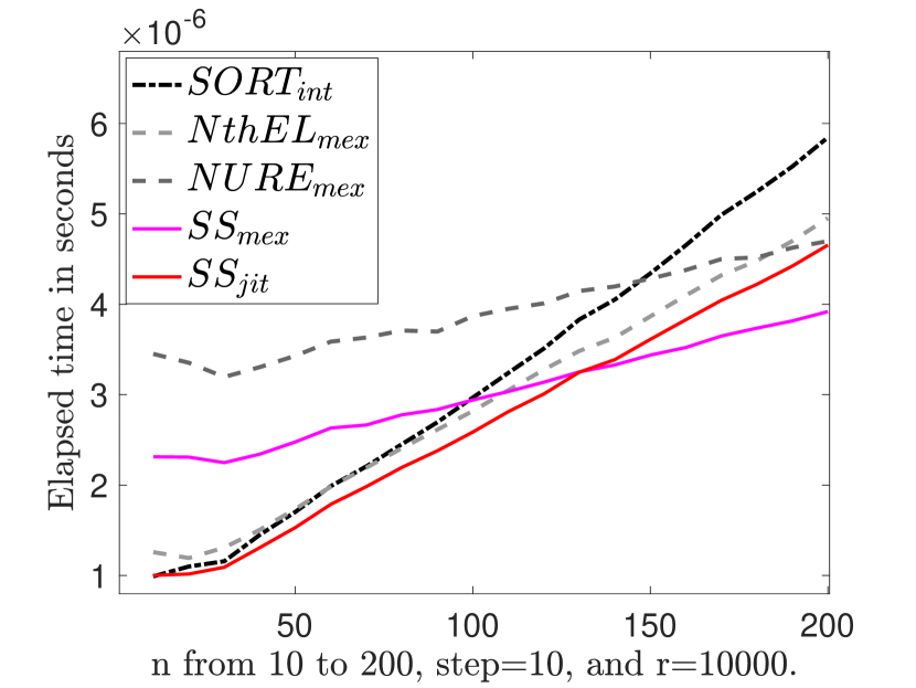
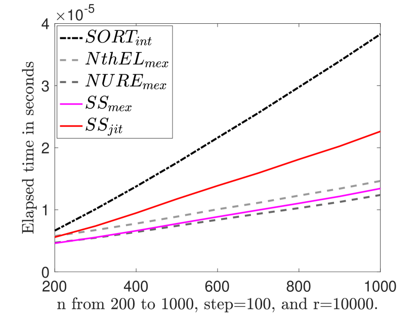
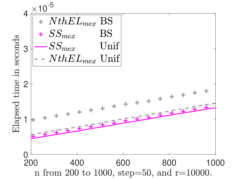
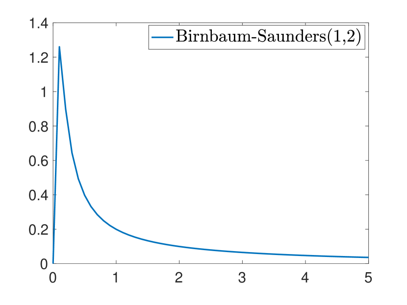
Figure 3: Finding the median. Top panels: elapsed time in seconds of simpleselect ($SS$), quickeselect as in Numerical Recipies in C ($NURE$), introselect as in the C++ nth_element function ($NthEL$) and the MATLAB-internal sort ($SORT$). Bottom-left panel: the ‘$+$’ symbols in gray and magenta refer respectively to introselect and simpleselect when $A$ is extracted from the Birnbaum-Saunders (BS) distribution on the bottom-right; the other two lines are obtained with the uniform distribution (Unif), as in the top panels.

The assessment is structured along the pseudo-code 1 (the actual code is available as supplementary material). The time results obtained for finding the lower median for $n$-values ranging between 10 and 1000, are reported in Figure 3 as median time over 10000 replicates. Therefore, the possibility of introducing a bias such as the potential initial latency of the jit compilation, is completely removed. The results show that:

1. Top panels. The plain MATLAB implementation of simpleselect ($SS_{jit}$) is competitive even for small sample sizes ($n<100$), but replacing the sort function provides limited time drop. The advantage increases considerably for larger sample sizes and becomes neat if the mex-compiled version is used; note also that its performance is in line with that of $NURE_{mex}$ and $NthEL_{mex}$.

2. Bottom panels. A key advantage of simpleselct, and comparable algorithms relying only on the pairwise order of the elements in $A$, is that performance is independent from the distribution of the data. On the contrary introselect, which tries to reach optimal worst-case performance by exploiting statistics (means and medians) on partitions of the data, may suffer from peaked data distributions like the one in the figure. [55] contains an extensive assessment exercise for a similar algorithm, the binmedian, which is indicative of the complications linked to the adoption of sophisticated solutions in real applications.

4 Use of selection in robust statistics

Many robust methods require order statistics to identify an outlier-free subset in a set of $p$-variate observations $X_{n}=\{x_{1},\ldots,x_{n}\}$. We illustrate with two case studies the advantages of adopting simpleselect for this purpose: in the first situation the required order statistic remains fixed at a same point (typically the median), while in the other it increases from $p+1$ to $n$ leaving, from a certain progression point, most of the largest values on the right side of the array.

Minimum Covariance Determinant (MCD).

The MCD tries to identify the subset of $h$ out of $n$ $p$-variate observations giving rise to the smallest determinant of the covariance matrix [52, 49]. The exact solution requires to evaluate ${n\choose h}$ cases, which in general is hard to compute being $(\frac{n}{k})^{k}\leq{n\choose h}\leq(\frac{en}{k})^{k}$ [15, p. 1186]. Fortunately the MCD has an approximate solution [50] that relies on taking at random many initial subsets and applying on each of them a fixed point iteration scheme with this property: if at step $t$ we have an $h$-subset $H_{t}$ with empirical mean and covariance matrix $\hat{\mu}_{t}$ and $\hat{\Sigma}_{t}$, and the (Mahalanobis) distance of observation $i$ is $d_{i}=d(x_{i},\hat{\mu}_{t},\hat{\Sigma}_{t})$, then the new $h$-subset $H_{t+1}$ formed by the observations with squared distances $d^{2}_{i}\leq d^{2}_{(h)}$ is such that $|\hat{\Sigma}_{t+1}|\leq|\hat{\Sigma}_{t}|$. Therefore, each iteration requires the computation of the order statistic $d_{(h)}$. Typically $h$ is set to $[(n+p+1)/2]$, which is around the median, and is possibly increased with a weighting step to improve the estimator’s efficiency. The initial random subset $H_{0}$ is of size $p+1$, which reduces the chance to embed outliers in computing the initial estimates $\hat{\mu}_{0}$ and $\hat{\Sigma}_{0}$. The loop continues until the equality condition on the determinant of the two covariance matrices is satisfied. Usually few iterations are sufficient to reach convergence, but the number of subsets to sample and iterate can be in the order of some thousands, and so are the applications of the appropriate order statistic computation.

Forward Search (FS)

The FS [3] adapts the value of $h$ to the data with an iteration procedure combined with a testing step. The iteration generates a sequence of parameter estimates, while the testing determines the $h$ value and detects the outliers on the basis of such parameters. More precisely, the iteration starts from a very robust fit to a few carefully selected observations, say $m_{0}=p+1$. Then it takes the $m_{1}=m_{0}+1$ observations with the smallest squared distances from the robust fit of $\hat{\mu}_{0}$ and $\hat{\Sigma}_{0}$. At step $m_{1}$ the parameter estimates are again computed and the process is iterated until all units are included ($m=n$). Therefore, each step of the iteration requires (i) a selection application to determine the $d_{(m+1)}^{2}$ smallest order statistic in the set of $i=1,\ldots,n$ distances computed on the basis of $\hat{\mu}_{m}$ and $\hat{\Sigma}_{m}$ and (ii) $n$ comparisons to identify the observations $i$ for which $d^{2}_{i}\leq d^{2}_{(m+1)}$. Therefore, there are $n-m_{0}+1$ steps requiring the computation of different (increasing) order statistics.

We illustrate the use of simpleselect in MCD and FS focusing on the potential benefit of its optional “oracle” parameter, which provides the index $j$ of an element in $A$ that might contain the desired $k$-th order statistic or be close to it. This option simply swaps $A(j)$ with $A(k)$ before starting the process; unless badly chosen, the initial guess on the pivot reduces the chance of falling into the worst case and improves the average case performance. For example, if at a certain FS step $m$ the variable minMDindex contains the index of the minimum of Mahalanobis distance among the units which form the group of potential outliers, then to increase by one unit the dimension of the basic subset bsb one could use option at line $9$ below where $j\leftarrow\mbox{{minMDindex}}$, instead of the standard simpleselect without oracle (line $6$) or the sort that we use as a baseline (line $3$):

⬇

1 switch bsb_update_by

2 case 'sort'

3 [$\sim$ , zsi] = sort(MD);

4 bsb = zsi(1:m+1);

5 case 'quickselectFS'

6 k=quickselectFS(MD,m+1);

7 bsb=(MD$\leq$k);

8 case 'quickselectFS_oracular'

9 k=quickselectFS(MD,m+1,minMDindex);

10 bsb=(MD$\leq$k);

11 end

In the MCD a similar approach is used in the iterative re-weighted least squares step, where the location and shape matrix are updated repeatedly till convergence. In this case we need to find the subset of $h$ observations with smallest covariance determinant and there is no counterpart to line $9$; the best we can try is to choose randomly a candidate between the units that are not in the current set of $h$ observations, as in line $12$ here:

⬇

12= quickselectFS(MD,h+1,h+1+randi(n-h-1,1,1));

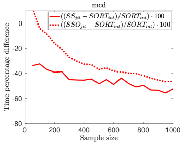
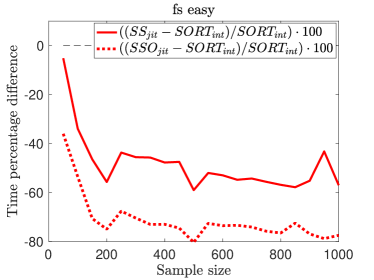
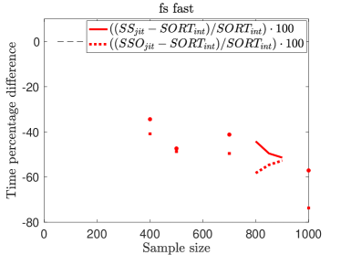
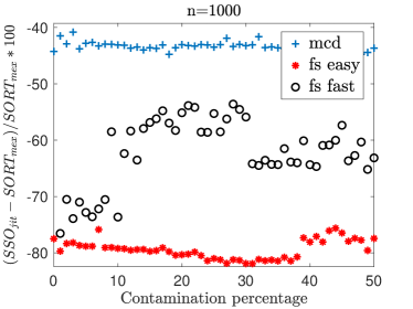
Figure 4: Effect of the oracular option of simpleselect in the MCD and two FS implementations, on data generated from a bi-variate normal distribution. Top and bottom-left panels: time percentage reduction w.r.t the SORT baseline with and without oracular option, for various sample sizes. Bottom-right panel: time reduction for fixed $n=1000$ and varying contamination level.

The top-left panel of Figure 4 shows that the random oracular choice does not help the MCD: in fact, the SSO curve is well above SS. For the FS the situation is reversed and the advantage of SSO is neat, but we have to distinguish between two implementations of the algorithm: one follows step by step the original FS formulation [2, 3] in the R package forward and the more recent FSDA function FSMmmdeasy.m; the other is a fast (but hardly readable) version of the algorithm [48] that in most of the forward steps updates the subset with logical operations instead of using sort or quickselectFS. The fast version – FSDA function FSMmmd.m – limits the application of quickselectFS to steps where more than one unit exit from the subset, the so called “interchange”. The effect is visible in the bottom-left panel of Figure 4, where the time information is available only episodically and for the larger $n$ values. However, the indication is that even in presence of interchange, and therefore uncertainty in the choice of $j$, the oracular option speeds up the method.

Given that the interchange increases if data are contaminated, we study the effect of creating two separate groups by adding a fixed shift to an increasing number of units in the normal bi-variate sample passed to MCD and the two FS implementations. As expected, the bottom-right panel of Figure 4 shows that the time gain in the MCD remains stable (towards $-40\%$), being the algorithm not subject to interchange by definition. In the fast FS the effect is strongest for small (up to $10\%$) contamination percentages and returns visible for large ones (above $35\%$); this is due to the fact that we initiate the FS with contaminated units, therefore initially we expect to fall in very unstable estimates and strong interchanges. In the standard FS the gain is remarkable (about $-80\%$) and increases as the contamination percentage approaches $40\%$; here the share due to the contamination is more difficult to appreciate, as most of the calls to quickselectFS do not depend on the interchange.

5 Extension to weighted selection

A number of statistical problems reduce to the selection of an order statistic on elements that are assigned with non-negative weights. For integer weights, this means choosing the order statistic from an increased set where each element is replicated to the number of the corresponding weight. We introduce the general problem focusing on the weighted median (Section 5.1), which is the 50% weighted percentile. We implement the weighted percentile as a natural extension of the simpleselect algorithm, in function quickselctFSw (Section 5.2). We illustrate its application to a computation-intense robust measure of skewness, the medcouple (Section 5.3).

5.1 Weighted median roots and applications

Finding the median $\tilde{A}$ defined in Section 1 also solves the optimization problem

$$\tilde{A}=\operatorname*{arg\!min}_{a}\sum_{i=1}^{n}|a_{i}-a|$$ (4)

Intuitively, the proof relies on the fact that the derivative with respect to $a$ of the sum of the absolute deviations is $\sum_{i=1}^{n}{\operatorname{sgn}(a_{i}-a)}$, which is zero only when the number of positive terms equals the number of the negative ones, which happens when $a$ is the median. If the absolute deviations are weighted by positive quantities $w_{i}$, then the minimization brings to the weighted median

$$\tilde{A}_{w}=\operatorname*{arg\!min}_{a}\sum_{i=1}^{n}w_{i}|a_{i}-a|$$ (5)

This optimization problem has fascinating historical roots in the least absolute deviation regression [54, 20], formulated already in 1760 by Boscovich and Simpson as a line minimizing the sum of the deviations of the observations from the line. Laplace, in his “Methode de Situation” (1818), indicated a solution for the line’s slope, finding that the weighted median solves the constrained least absolute deviation regression obtained by replacing in (5) $w_{i}=|x_{i}-\overline{x}|$ and $a_{i}=(y_{i}-\bar{y})/(x_{i}-\bar{x})$, being $(x_{i},y_{i})$, $i=1,\ldots,n$, a two-dimensional sample of points with one independent and one dependent variables respectively. Laplace understood that $\tilde{A}_{w}$ in (5) is equal to $a_{(k^{*})}$, with $k^{*}$ found by considering the order statistics of the weights $w_{(i)}$ and returning the smallest $k$ associated with the weight whose running sum crosses $50\%$ of the total weight, that is:

$$k^{*}=\min\left\{k\mathrel{}\middle|\mathrel{}\sum_{i=1}^{k}w_{(i)}\geq\frac{1}{2}\sum_{i=1}^{n}w_{i}\right\}$$ (6)

The problem found consolidation with the “double median” of [19] (the solution for the intercept) and a century later with the simplex algorithm [6, 9]. Modern concepts that revisit and extend these ideas are the “dual plot” and “regression depth” by [51] and the robust time series smoothing and filtering by [16, 23].

The weighted median and percentiles find intriguing test cases also in engineering and machine learning, where disposing of efficient algorithms is essential for large-scale applications. For example, non-linear digital filtering devices embed weighted percentiles for noise cancellation [1, 56], while medical experiments use them when the precision of individual estimates varies considerably [11]. In machine learning it is interesting the case of boosting procedures, which aim generating an accurate prediction by combining several weaker estimators (statistics treats the case in the additive models theory [24]). The original formulation of boosting by [22] proposes to build the final prediction as weighted average of the individual models, but also shows that the optimal prediction in regression (AdaBoost.R2) should be based on the weighted median of the weak learners. Additional motivations for the weighted median were given by [35, 36] in view to achieve a certain degree of robustness and by [7] for responses in $[0,1]$. Recently, [4] have shown an application of that approach to sensitivity analysis, where predictions (and therefore weighted medians) have to be computed a great number of times.

5.2 Weighted simpleselect

The value $k^{*}$ of equation 6 is returned by function quickselctFSw (listing 2, output variable kstar) with the input parameter $p=0.5$, that is the percentile $100p=50\%$. More in general, for a generic percentile $100p\in[0,100]$, the function returns a value $k^{*}_{p}$ and a permutation of the weights which forces the sum of weight partition around $k^{*}_{p}$ to be as equal as possible and therefore the following difference as small as possible:

$$\sum_{i=1}^{k^{*}_{p}-1}w_{i}-\sum_{i=k^{*}_{p}+1}^{n}w_{i}.$$ (7)

The histogram in the top-right panel of Figure 5 shows that the resulting objective function values (5) are identical in quickselctFSw and an optimal $\mathcal{O}(n\log{}n)$ solution [29], which sorts the weights for finding the smallest ones summing to half the total weights (respectively SSw and WMsort in the legend). The top-left panel of the same figure shows that our $\mathcal{O}(n)$ solution is advantageous even for small $n$, which is remarkable considering that it is obtained also here without compiling the code. The plot also shows that the $\mathcal{O}(n\log n)$ solution when $n$ is in the order of some thousands becomes very impractical. Finally, the bottom-left panel shows that our extension to a generic weighted percentile works as expected, that is, for uniformly distributed weights the positions $k^{*}_{p}$ returned by quickselctFSw are very close to the desired input percentile $100p$.

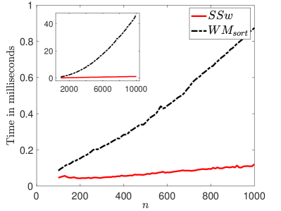
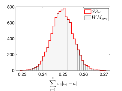
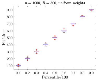
Figure 5: Weighted simpleselect (SSw) and a $\mathcal{O}(n\log{}n)$ solution [29] (WMsort). Top-left: elapsed time for a weighted median, for $n\in[100,10000]$. Top-right: objective function values for weights and data from $U(0,1)$ and $n=1000$. Bottom-left: positions $k^{*}_{p}$ returned in kstar by quickselctFSw for various percentiles $100p$ and $n=1000$.

The code listing 2 for quickselctFSw is obtained as a natural extension of quickselctFS. It is sufficient to embed the core part of the listing 1 in a loop (starting at line 9) that checks the status of the sum or weights partition (7) by extending the weighted median approach by [8]. The core part of quickselctFS (lines 11-33) is called on the data assuming that the weighted percentile is in position $k=\lceil np\rceil$ (line 6). This first iteration permutes vector D so that the weights at positions $(1:k-1)$ are smaller than the $k$th weight. At this point we check whether the array fulfills the weights balance (lines 36, 37, 41). If so, we stop iterating (line 39). If not, we apply again the core part of quickselctFS on either $D(1:k,:)$ with $k+1$, or $D(k:n,:)$ with $k-1$. The iteration will remove or add weights in order to approach the optimal condition.

The code spends most of the time - between 60% and 70% - in swapping rows (lines 19-20-21) within the loop at lines 16-25. As the cell-pairs to swaps are expected to follow the column major order of the MATLAB matrices, we traverse first the data elements D(:,1), which internally will be contiguous in memory, and then the weights elements D(:,2). This cell-wise swap approach is indeed found much faster than the conventional full-row swap of instructions

buffer=D(i,:);     D(i,:)=D(position,:);     D(position,:)=buffer;

Finally note that in general the point that sum exactly to $100p\%$ of the total weight is between two data values. Therefore, at line 37 two values of $k$ can make D(k,2) to satisfy equation (7). We decided to solve the tie by returning the minimum between the two. In the case of the 50% percentile, this is the lower weighted median. This has to be taken into account when comparing quickselctFSw with solutions opting for the upper weighted median or an interpolant between the two, such as the mean.

Listing 2: Code distilled from quickselectFSw.m. Also available as R, C and C-mex files.

⬇

1ction [kD , kW , kstar] = quickselectFSw(D,W,p)

2% Extends SimpleSelect to weighted order statistics

3

4n=length(D); left = 1; right = n; position=-1;

5D=[D(:),W(:)]; % Values & weights go in pairs

6k=ceil(n*p); % Pivot index set to work in D(1:k,:)

7

8BleichOverton = true; %%% The external loop checks %%%

9while BleichOverton %%% the condition on weights %%%

10

11 while (position$\sim$=k) % Internal loop is quickselectFS

12 pivot = D(k,:); %|

13 D(k,:) = D(right,:); %| row swap

14 D(right,:) = pivot; %|

15 position = left;

16 for i=left:right

17 if (D(i,1)<pivot(1,1))

18 for s=1:2 %|

19 buffer = D(i,s); %| cell-wise

20 D(i,s) = D(position,s); %| row swap

21 D(position,s) = buffer; %|

22 end %|

23 position = position+1;

24 end

25 end

26 D(right,:)=D(position,:);

27 D(position,:)=pivot;

28 if (position < k)

29 left = position + 1;

30 else

31 right = position - 1;

32 end

33 end

34

35 %%% Checks on weights - extends Bleich-Overton %%%

36 Le=sum(D(1:k-1,2));

37 if Le-p$\leq$0 && p-Le-D(k,2)$\leq$0 %% OK: stop computation

38 kD=D(k,1); kW=D(k,2); kstar=k;

39 BleichOverton=false;

40 else %% NOT OK: go back to quickselectFS

41 if D(k,2)<2*(p-Le) % Need to add a weight

42 k=k+1; left=k; right=n;

43 else % Need to remove a weight

44 k=k-1; left=1; right=k;

45 end

46 end

47 position=-1;

48end

5.3 Application to the fast medcouple

The weighted median is heavily used by a fast algorithm for the medcouple [13], a robust measure of skewness used to adjust the whiskers of a boxplot [33] and avoid wrong declaration of outliers in asymmetric univariate data. The R package robustbase (https://cran.r-project.org/web/packages/robustbase) and the MATLAB toolbox LIBRA (http://wis.kuleuven.be/stat/robust.html) implement the fast medcouple with wrapper functions to the same compiled C source, to maximize speed. We have replicated faithfully the C function mlmc.c in a pure MATLAB function, medcouple.m, but we have replaced the computations of the median and weighted median with calls to our functions quickselectFS and quickselectFSw or, for comparison, the $\mathcal{O}(n\log n)$ solution by [29]. For completeness, medcouple.m has been enriched with options to compute a “naive” $\mathcal{O}(n^{2})$ solution and the quantile and octile approximations used by [13] for comparison. The consistency between mlmc.c in C and medcouple.m in MATLAB has been ensured with systematic checks, ensuring same random numbers generation with the Mersenne Twister framework. In Annex A.4 we show how this is done and introduce a function to replicate random numbers also in R, which is not obvious.

	Medcouple function	$\mathbf{n=10000}$	$\mathbf{n=1000}$	$\mathbf{n=100}$
1	mlmc.c (full C-compiled)	0.5272	0.0384	0.0114
	medcouple.m (full matlab-interpreted) with calls to:
2	- quickselectFSw (mex)	1.4456	0.0657	0.0170
3	- quickselectFSw (jit)	3.5361	0.1100	0.0155
4	- weightedMedian (jit/sort)	14.5733	0.2823	0.0272
5	- naive (jit/sort)	35.1412	0.1633	0.0073

Table 1: The medcouple with different weighted median solutions. Total time in seconds to apply the medcouple to 100 random samples of different size drawn from a log-normal distribution with function lognrnd(0,1,n,1).

Table 1 gives an idea of the relative performance of the various solutions. Our baseline (row 1) is the run with the fully-compiled mlmc.c, which is obviously advantaged. However, given that the algorithm spends most of the time in computing weighted medians, we expect comparable performances when medcouple.m uses the C-compiled mex of quickselectFSw (row 2). The reported result is in accordance with expectancy, but note that this option could run faster by refining for speed the C-code of quickselectFSw and replacing the loops in medcouple.m with vectorized code. Note finally that using the standard matlab function quickselectFSw.m (row 3) doubles the overall execution time (for medium-large $n$), yet keeping far from the time required by naive solutions based on sorting (rows 4 and 5): the need of avoiding them is obvious.

5.4 Application in digital filtering

Digital filtering covers many applications; here we take as an example the denoising of raster images, which was originally done by taking a number of values around a pixel and replacing it with the median of these values [45]. The procedure is repeated within a window sliding throughout the image. [12] has shown that the weighted median works better, especially to remove specific structural patterns. Obviously in this process the weighted median is used a very large number of times, depending on the image resolution. The listing 3 shows that the calls to quickselectFSw.m would be $(row-3)\cdot(col-3)\cdot rgb=4,604,862$ for a $3\times 3$ weight mask and a $1280\times 1205\times 3$ photo like the one in Figure 6

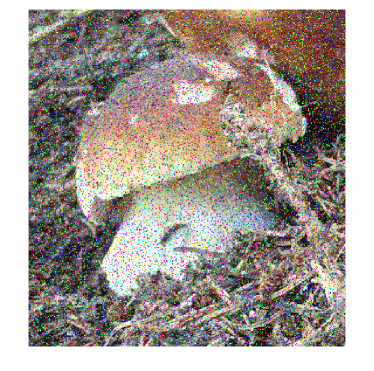
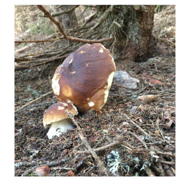
Figure 6: A $1280\times 1205\times 3$ pixels photo denoised with the weighted median using a Wiener filter mask $W=[10,12,9\,\,;\,12,19,12\,\,;\,9,12,10]$. The detail on the left panel shows the added noise, which is removed by the filter (right panel).

where we added a certain percentage of gaussian noise. If we replace at line 36 the call to quickselectFSw.m with the weighted median,

⬇

36 , Zclean(ind5)] = weightedMedian(A,W);

which relies on sort, the time execution raises more than 4 times (from 16 to 66 seconds in our test), which is a lot considering that in this case the weighted median is executed repeatedly on a small array of 9 values where the gain of replacing sort with quickselectFSw is in principle very limited.

Listing 3: Use of quickselectFSw.m to denoise a photo.

⬇

1ile = 'boletus1280.jpg';

2pnoise = 0.2; % percentage of noise to add

3

4I = imread(imfile); % read image

5%I = rgb2gray(I); % uncomment for black and white

6Z = double(I);

7[row , col , rgb] = size(Z);

8

9%% add noise to the image

10x = rand(size(Z));

11d = x < pnoise/2;

12Z(d) = 0; % Set to minimum value

13d = find(x $\geq$ pnoise/2 & x < pnoise);

14Z(d) = 255; % Set to saturated value

15

16%% Weight-mask for the Wiener filter

17W = [10,12,9; 12,19,12; 9,12,10];

18W = W ./ sum(sum(W)); W = W(:);

19

20%% denoise with weighted median

21% requires (col-3)*(row-3)*rgb calls to quickselectFSw

22Zclean = Z(:);

23for qsw=0:1

24 for y = 2:1:(col-1)*rgb

25 for x = 2:1:row-1

26 ind1 = x-1 + (y-1 - 1).*row;

27 % = sub2ind([row,col],x-1,y-1);

28 ind2 = x-1 + (y - 1).*row;

29 % = sub2ind([row,col],x-1,y);

30 ind3 = x-1 + (y+1 - 1).*row;

31 % = sub2ind([row,col],x-1,y+1);

32 ind5 = x + (y - 1).*row;

33 % = sub2ind([row,col],x,y);

34 imask = [ind1; ind1+1; ind1+2; ind2; ind2+1; ind2+2; ind3; ind3+1; ind3+2];

35 A = Z(imask);

36 Zclean(ind5) = quickselectFSw(A,W,0.5);

37 end

38 end

39end

40Zclean = reshape(Zclean,size(Z));

41figure; imshow(uint8(Zclean))

6 Conclusion

Forty years ago [8] observed with a certain surprise that the best known linear algorithms for computing the median and weighted median can take in practice more CPU time than the “naive” counterparts based on sorting, even for arrays of several thousands elements. This happens because of a constant but not negligible level of complexity linked to impractical data structures or problematic heap or stack memory management issues proper of intricate algorithms. It is therefore comprehensible that linear selection algorithms are hard to find in the main distribution of many statistical and programming environments. As for weighted percentiles, to our knowledge the offer covers generally the weighted median and rarely with linear complexity solutions. We have shown that in robust statistics still today it can be convenient to resort to (weighted) selection algorithms and that our simplifications and generalizations neutralise the constant computational overhead.

The software necessary to replicate the results in the paper is available in https://github.com/UniprJRC/FSDApapers, under the folder simpleselect /ArticleReplicabilityCodes. We provide the key functions quickselectFS and quickselectFSw as MATLAB, R, C and C-mex sources, the latter also compiled as binary mex files for the Linux, MacOsX and MS-Windows platforms. These functions are also hosted by the standard distribution of FSDA, which can be downloaded from the GitHub space UniprJRC as well. The R community and users of other open environments like Python may run FSDA tools through the (automatically generated) C-codes and the corresponding R-wrappers available in the GitHub projects FSDA-MATLAB_Coder and fsdaR [25].

Appendix A Appendices

A.1 Expected increments of position in simpleselect

In Listing 1, the ‘for loop’ is initialised with position=left=1 and right=n and receives a certain pivot value $a$ from the outer ‘while loop’. Then, $a$ is compared with all elements of $A$, assumed to originate from its same (unknown) parent distribution. Given that $a$ is taken from the element $a_{k}\in A$ (line 8), the pivot is actually compared with the $N=n-1$ elements of $A\setminus\{a_{k}\}$ with the following $N+1$ possible outcomes:

$$a\leq a_{(1)}\quad;\quad a_{(1)}<a\leq a_{(2)}\quad;\quad\ldots\quad;\quad a_{(N-1)}<a\leq a_{(N)}\quad;\quad a>a_{(N)}$$ (8)

The last outcome obviously occurs when $a_{k}=a_{(n)}$. If we think about $A$ as one of $L$ independent samples analysed each by simpleselect, we can use a statistical extreme value problem formulated by [28, Lecture 2, Plotting Positions] on the cumulative distribution $F(a_{(m)})$ of the $m$-th smallest value among $N$ observations, stating that:

$$P(a\leq a_{(m)})=\lim_{L\rightarrow\infty}r_{L}(a\leq a_{(m)})=\lim_{L\rightarrow\infty}F(a_{m:L})=E(F(a_{(m)}))=\frac{m}{N+1}$$ (9)

where $r_{L}(\cdot)$ denotes the relative cumulative frequency computed on the $L$ samples and $a_{m:L}$ the set of $L$ individual $m$th ranked values $a_{(m)}$. Note that the cdf (9) is a step function increasing by $\frac{1}{N+1}$ in each of the $N+1$ intervals representing the outcomes of (8). This also means that $P(a=a_{(m)})=\frac{1}{N+1}$ independently from $m$. A compact demonstration of (9) with discussion on related results, can be found in [41].

Now, consider the subset of $A$ formed by the elements that satisfy the ‘if statement’ at line 18 and make position to increment by 1. We can denote the subset with $A_{lr}=\{a_{i}<a\;;\;i=l,\ldots,r\}$, $l$ and $r$ being respectively the indexes of the left and right pointers. The expected number of increments of position is the mean of the random variable $X=|A_{l,r}|$, which we derive here for the first iteration of simpleselect, where:

$$X=|A_{1,n}|=t\quad\mbox{if}\;a=a_{(t+1)}\quad\mbox{for}\;t=0,1,\ldots,N$$

Given that the cdf (9) implies $\;P(X=t)=\frac{1}{N+1}$ independently from $t$, we have:

$$E[X]=\sum_{t=0}^{N}t\cdot P(X=t)=\frac{1}{N+1}\sum_{t=1}^{N}t=\frac{N(N+1)}{2(N+1)}=\frac{N}{2}=\frac{n-1}{2}$$ (10)

A.2 Implementation of the Vervaat perpetuities

A perpetuity is a random variable of the form:

$$Y=W_{1}+W_{1}\cdot W_{2}+W_{1}\cdot W_{2}\cdot W_{3}+\ldots$$

where the $W_{i}$ are an independent, identically distributed sequence of random variables. If each $W_{i}$ has the same distribution, say $W_{i}\sim W$, then $Y\sim W(1+Y)$ for $Y$ and $W$ independent. The comparisons of Hoare’s Find are distributed asymptotically as a particular perpetuity called Dickman, with $W\sim Unif([0,1])$. Unfortunately such distribution has no closed form.

The Dickman can be also seen as a special case of Vervaat perpetuity, which is such that $W_{i}\sim U^{1/\beta}$ for some $\beta\in(0,\infty)$ for $U\sim Unif([0,1])$. In other words, the Dickman distributon is a Vervaat perpetutiy with $\beta=1$. A generalization of the perpetuity takes the form

$$Y=\sum_{n=0}^{\infty}A_{n}\prod_{i}^{n}W_{i}$$

with $A_{n}$ not necessarily equal to $1$, which is known as Takacs distribution. Our implementation of the Vervaat family (vervaatxdf.m) (listing 4) follows [5], who introduced a feasible and elegant method for computing the probability density and distribution functions that avoids brute force simulation (code by the authors exists in Wolfram’s Mathematica). For comparison we also ported from R to MATLAB the recursive simulation approach of [14], which is accurate but much slower (vervaatsim.m). For completeness, we implemented a function to simulate random variates from the Vervaat (vervaatrnd.m), using one of the two methods above.

Listing 4: Code distilled from the FSDA toolbox. Follows Wolfram’s Mathematica code kindly shared with us by [5]. User documentation: http://rosa.unipr.it/FSDA/vervaatsim.html.

⬇

1ction [f , F , x] = vervaatxdf(betav,nx,pascalM)

2%pdf and cdf of a Vervaat perpetuity.

3% betav : Distribution parameter value.

4% nx : Number of evaluation points.

5% pascalM: A precomputed Pascal matrix, used to speed up things in simulations. Remark: bc(a,b) = pascalM(a-b+1,b+1).

6

7eulerGammaval = 0.577215664901532860606512090082402431;

8n = 100;

9if nargin==0, betav = 1; end; % default is a Dickman

10if nargin<2, nx = 1; end;

11if nargin<3, pascalM = pascal(n+1); end;

12

13h = zeros(1,n);

14L = zeros(1,n+1);

15ex = 5*betav;

16x = ex.*rand(1,nx); %nx random numbers from U in [0,ex]

17f = zeros(1,nx);

18F = zeros(1,nx);

19

20for k=1:nx

21 s=n/x(k);

22 h(1) = betav * (exp(-s) - 1)/s;

23 for j=2:n

24 h(j) = (betav / s) * (-1)^(j-1) * exp(-s) - ((j-1)/s * h(j-1)) ;

25 end

26 L(1) = exp(betav * (- eulerGammaval - gammainc(0,s) - log(s) ));

27 for i=2:n+1

28 Li = 0;

29 for j=0:i-2

30 Li = Li + pascalM(i-2-j+1,j+1) * h(i-1-j) * L(j+1);

31 %Li = Li + bc(i-2,j) * h(i-1-j) * L(j+1);

32 end

33 L(i) = Li;

34 end

35 % pdf

36 f(k) = ( (-1)^n / factorial(n) ) * s^(n+1) * L(n+1);

37 % cdf

38 F(k) = sum((-s).^(0:n) ./ factorial(0:n) .* L((0:n)+1));

39end

A.3 Call quickselectFS.c and quickselectFSw.c from Python

All statistical programming environments can integrate C functions to eliminate performance bottlenecks or compute specific algorithms. The typical approach is to write a code in the environment in use (the wrapper) that maps the original data types to those in the C code, initializes the function parameters and captures the result from the call to the compiled C function. The code listing 5 illustrates how quickselectFS.c can be called from Python. The call to quickselectFSw.c is similar.

Listing 5: A wrapper calling quickselectFS.c from Python.

⬇

1# This Python script illustrates an easy way to call

2# quickselectFS.c from Python, passing a Numpy array

3# as the first argument.

4#

5# The .c source file should be compiled as follows:

6#

7# gcc -fPIC -shared -o simpleselect.so simpleselect.c

8#

9# The C-compatible data types are built by the

10# foreign Python function library ctypes.

11

12import ctypes

13from numpy.ctypeslib import ndpointer

14import numpy as np

15

16lib = ctypes.cdll.LoadLibrary("simpleselect.so")

17quickselectFS = lib.quickselectFS

18

19quickselectFS.restype = ctypes.c_double

20quickselectFS.argtypes = [ndpointer(ctypes.c_double, flags="C_CONTIGUOUS"),

21 ctypes.c_int,

22 ctypes.c_int]

23

24A = np.arange(-5.0, 6.0, 1, dtype = float)

25print(A)

26np.random.shuffle(A)

27

28# quickselectFS works in-place, so we have to create a copy of vector A if we want to retain the original A.

29

30aux = A.copy()

31

32k = 7

33k_th_ord_stat = quickselectFS(aux, len(aux), k)

34

35print(k_th_ord_stat)

36

37del aux

A.4 Generating same random numbers in MATLAB, C and R

To generate same random numbers in different languages just requires, in principle, the adoption of the same generation method. A famous one is the Mersenne Twister algorithm by [43], which is available for various languages at http://www.math.sci.hiroshima-u.ac.jp/m-mat/MT/emt.html. The code listing 6 illustrates how to use it in C to create from a given seed an array $D$ of uniform random numbers in $[0,1)$, and apply on it quickselectFS. To replicate these numbers in MATLAB from the same seed is easy, as it includes since 2005 (R14SP3) built-in support for the Mersenne Twister mt19937ar. It is sufficient to run:

⬇

RandStream.setGlobalStream(RandStream.create('mt19937ar','seed',896));

D = rand(n,1);

or equivalently

⬇

myseed = 896; rng(myseed , 'twister');

D = rand(n,1);

Note that instructions below produce the same $n$ integers between 1 and $N$

⬇

D = ceil(rand(n,1)*N); D = randi(N,n,1);

that is, we can easily obtain uniform integers from uniform floats.With Python the approach is similar, as it has the Mersenne Twister as core generator with the same underlying C library.

Listing 6: Generate same random numbers with Mersenne Twister: C-side.

⬇

1clude <stdio.h>

2#include <stdlib.h>

3#include <stdint.h>

4#include <math.h>

5#include "simpleselect.h" // quickselectFS/quickselectFSw

6#include "mersenne.h" // mt19937ar, Mersenne Twister

7 // with improved initialization

8int main() {

9 int n, k;

10 printf("\n Choose sample size n: ");

11 scanf("%d",&n);

12 printf("\n Choose order statistic k ($\leq$n): ");

13 scanf("%d",&k);

14 double D [n];

15

16 uint32_t seed = 896; // set a seed

17 init_genrand(seed); // initialise mt[n] with seed

18 for (int i=0; i<n; ++i) { // generates random number in [0,1)

19 D[i] = genrand_res53(); // with 53-bit resolution

20 }

21

22 double wE =quickselectFS(D,n,k-1); // apply quickselectFS

23 printf("\n result: %f\n", wE);

24 return 0;

25}

Instead, to replicate the same numbers in R is much more difficult, because the seeding algorithm in R does not follow exactly mt19937ar, using a different initialization and output transformation. This makes impossible, to our knowledge, to map directly R seed values to MATLAB/C’s. The R package randtoolbox offers an option aimed to generate random numbers along mt19937ar:

⬇

set.generator("MersenneTwister", initialization="init2002", resolution=53, seed=myseed)

If, following the manual, we run it in R (V 4.0.5) with myseed=12345, we get

⬇

> runif(5)

[1] 0.1839188 0.2045603 0.5955447 0.6531771 0.2987037

Unfortunately, the manual reports a different sequence, which indeed we get in MATLAB with:

⬇

>> rand('twister', myseed); rand(1, 5)

ans =

0.9296 0.3164 0.1839 0.2046 0.5677

It seems therefore that the behavior of randtoolbox is not stable.

For this reason, we have integrated in FSDA a new function mtR.m that generates the same uniformly or normally distributed random numbers produced by the base R with mt19937ar. As it is not possible to map R seeds into MATLAB’s ones, the starting point of mtR.m is the 626-element int32 vector containing the random number generator state used by R to generate random numbers, which we can get by executing:

⬇

RNGkind("Mersenne Twister") # set "Mersenne Twister" "Inversion"

set.seed(myseed)

Rstate = .Random.seed

Of course, rather than generating in R a 626-element vector and pass it to mtR.m in MATLAB, it would be more convenient to build directly inside MATLAB the R state vector corresponding to a valid R seed. Fortunately, this is possible following the Mersenne Twister’s C code, which we have introduced in mtR.m in the form of Listing 7.

Listing 7: Generate same random numbers with Mersenne Twister: MATLAB-side. Sub-functions used by mtR.m to initialize the R state from a given seed. They mimic the Mersenne Twister’s C code.

⬇

1ction state = initMT_R(seed)

2% Create an initial R Mersenne Twister state from a seed.

3% c.f. RNG_Init() in RNG.c.

4n = double(seed); % in case it was given as an int32

5state = zeros(626,1,'int32');

6for i = 1:50, n = int32lcg(n); end

7for i = 2:626

8 n = int32lcg(n);

9 state(i) = n;

10end

11state(1) = 403;

12state(2) = 624;

13end

14

15function n = int32lcg(n)

16% Mimic the old glibc LCG that R uses for MT initialization,

17% in int32 arithmetic (MATLAB's int32 saturates, C's wraps).

18% c.f. RNG_Init() in RNG.c.

19n = 69069 * n + 1;

20if n $\geq$ 2^31 || n < -2^31

21 n = mod(n+2^31,2^32) - 2^31;

22end

23end

At this point, mtR.m can digest the generated R state by eliminating the first code, which stands for the RNG algorithm, reshuffling the state in the standard MATLAB form and recasting the vector from the signed integers used by R to the unsigned counterparts used by MATLAB; in short:

⬇

Rstate = initMT_R(myseed);

MATLABstate = [Rstate(3:end); Rstate(2)];

MATLABstate = typecast(int32(MATLABstate),'uint32');

Now, we can get MATLAB’s current global random number stream and set the state to that converted for R (or received directly from R if convenient):

⬇

Mstream = RandStream.getGlobalStream();

Mstream.State = MATLABstate;

The last trick to keep in mind is to use the inverse transformation to compute a normal random variate (i.e. the standard normal inverse cumulative distribution function is applied to a uniform random variate). This replaces the MATLAB default, which is the ziggurat algorithm [42].

Function mtR.m contains numerous MATLAB/R examples, which can be used in simulation exercises involving both languages.

References

- Astola and Kuosmanen [1997] J. Astola and P. Kuosmanen. Fundamentals of Nonlinear Digital Filtering. CRC Press, 1st ed. edition, 1997. doi: 10.1201/9781003067832.
- Atkinson and Riani [2000] A. C. Atkinson and M. Riani. Robust Diagnostic Regression Analysis. Springer-Verlag, New York, 2000. doi: 10.1007/978-1-4612-1160-0.
- Atkinson et al. [2004] A. C. Atkinson, M. Riani, and A. Cerioli. Exploring Multivariate Data with the Forward Search. Springer–Verlag, New York, 2004. doi: 10.1007/978-0-387-21840-3.
- Azzini et al. [2022] I. Azzini, T. Mara, and R. Rosati. A novel boosting algorithm for regression problems (bOOstd) and its use for sensitivity analysis. 10th International Conference on Sensitivity Analysis of Model Output, March 2022.
- Barabesi and Pratelli [2019] Lucio Barabesi and Luca Pratelli. On the properties of a takács distribution. Statistics & Probability Letters, 148:66–73, 2019. ISSN 0167-7152. doi: 10.1016/j.spl.2019.01.005.
- Barrodale and Roberts [1973] I. Barrodale and F. D. K. Roberts. An improved algorithm for discrete linear approximation. SIAM Journal on Numerical Analysis, 10(5):839–848, 1973.
- Bertoni et al. [1997] Alberto Bertoni, Paola Campadelli, and M. Parodi. A boosting algorithm for regression. In Proceedings of the 7th International Conference on Artificial Neural Networks, ICANN ’97, page 343–348, Berlin, Heidelberg, 1997. Springer-Verlag. ISBN 3540636315. doi: 10.1007/bfb0020178.
- Bleich and Overton [1983] Chaya Bleich and Michael L. Overton. A linear-time algorithm for the weighted median problem. Technical Report 75, New York University, Courant Institute of Mathematical Sciences, April 1983.
- Bloomfield and Steiger [1980] Peter Bloomfield and William Steiger. Least absolute deviations curve-fitting. SIAM Journal on Scientific and Statistical Computing, 1(2):290–301, 1980. doi: 10.1137/0901019.
- Blum et al. [1973] Manuel Blum, Robert W. Floyd, Vaughan Pratt, Ronald L. Rivest, and Robert E. Tarjan. Time bounds for selection. Journal of Computer and System Sciences, 7(4):448 – 461, 1973. ISSN 0022-0000. doi: 10.1016/s0022-0000(73)80033-9.
- Bowden et al. [2016] Jack Bowden, George Davey, Philip Haycock, and Stephen Burgess. Consistent estimation in mendelian randomization with some invalid instruments using a weighted median estimator. Genetic Epidemiology, 40(4):304–314, 2016. doi: 10.1002/gepi.21965.
- Brownrigg [1984] D.R.K. Brownrigg. The weighted median filter. Communications of the ACM, (27):807–818, 1984. doi: 10.1145/358198.358222.
- Brys et al. [2004] G Brys, M Hubert, and A Struyf. A robust measure of skewness. Journal of Computational and Graphical Statistics, 13(4):996–1017, 2004. doi: 10.1198/106186004X12632.
- Cloud and Huber [2017] Kirkwood Cloud and Mark Huber. Fast perfect simulation of vervaat perpetuities. Journal of Complexity, 42:19–30, 2017. doi: 10.1016/j.jco.2017.03.005.
- Cormen et al. [2009] Thomas H. Cormen, Charles E. Leiserson, Ronald L. Rivest, and Clifford Stein. Introduction to Algorithms, Third Edition. The MIT Press, 3rd edition, 2009.
- Davies et al. [2004] P.L Davies, R. Fried, and U. Gather. Robust signal extraction for on-line monitoring data. Journal of Statistical Planning and Inference, 122(1):65 – 78, 2004. doi: 10.1016/j.jspi.2003.06.012.
- Dor and Zwick [1995] Dorit Dor and Uri Zwick. Selecting the median. In Proceedings of the Sixth Annual ACM-SIAM Symposium on Discrete Algorithms, SODA ’95, pages 28–37, Philadelphia, USA, 1995. Society for Industrial and Applied Mathematics. ISBN 0-89871-349-8. doi: 10.1137/s0097539795288611.
- Dromey [1986] R. Geoff Dromey. An algorithm for the selection problem. Software: Practice and Experience, 16(11):981–986, 1986. doi: 10.1002/spe.4380161103.
- Edgeworth [1888] F.Y. Edgeworth. XXII. on a new method of reducing observations relating to several quantities. The London, Edinburgh, and Dublin Philosophical Magazine and Journal of Science, 25(154):184–191, 1888.
- Farebrother [1990] W. R. Farebrother. Studies in the history of probability and statistics XLII. further details of contacts between boscovich and simpson in june 1760. Biometrika, 77(2):397–400, 06 1990. doi: 10.1093/biomet/77.2.397.
- Fisher and Yates [1948] Sir Fisher, Ronald Aylmer and Frank Yates. Statistical tables for biological, agricultural and medical research. London: Oliver and Boyd, 3rd ed edition, 1948. doi: 10.2307/1905265.
- Freund and Schapire [1997] Y. Freund and R.E. Schapire. A decision-theoretic generalization of on-line learning and an application to boosting. Journal of Computer and System Sciences, 55(1):119–139, 1997. ISSN 0022-0000. doi: 10.1006/jcss.1997.1504.
- Fried et al. [2007] Roland Fried, Jochen Einbeck, and Ursula Gather. Weighted repeated median smoothing and filtering. Journal of the American Statistical Association, 102(480):1300–1308, 2007. ISSN 01621459. doi: 10.1198/016214507000001166.
- Friedman et al. [2000] Jerome Friedman, Trevor Hastie, and Robert Tibshirani. Additive logistic regression: a statistical view of boosting (With discussion and a rejoinder by the authors). The Annals of Statistics, 28(2):337–407, 2000. doi: 10.1214/aos/1016218223.
- FSDA [2005-2021] FSDA. Flexible Statistics & Data Analysis toolbox for MATLAB, with extensions to R and SAS. GitHub: https://github.com/UniprJRC/FSDA; Matlab Central File Exchange: https://www.mathworks.com/matlabcentral/fileexchange/72999-fsda; Documentation: http://rosa.unipr.it/FSDA/guide.html, 2005-2021.
- Giuliano et al. [2018] R. Giuliano, Z.S. Szewczak, and M.J.G Weber. Almost sure local limit theorem for the Dickman distribution. Periodica Mathematica Hungarica, 76:155 – 197, 2018. doi: 10.1007/s10998-017-0193-0.
- Goldstein [2018] Larry Goldstein. Non-asymptotic distributional bounds for the Dickman approximation of the running time of the Quickselect algorithm. Electronic Journal of Probability, 23:1–13, 2018. doi: 10.1214/18-EJP227.
- Gumbel [1954] E.J. Gumbel. Statistical Theory of Extreme Values and Some Practical Applications: A Series of Lectures. Applied mathematics series. U.S. Government Printing Office, 1954.
- Haase [2022] Sven Haase. Weighted median. MATLAB Central File Exchange, December 2022. URL https://www.mathworks.com/matlabcentral/fileexchange/23077-weighted-median.
- Hoare [1961a] C. A. R. Hoare. Algorithm 64: Quicksort. Communications of the ACM, 4(7):321, 1961a. doi: 10.1145/366622.366644.
- Hoare [1961b] C. A. R. Hoare. Algorithm 65: Find. Communications of the ACM, 4(7):321–322, 1961b. doi: 10.1145/366622.366647.
- Hoare [1971] C. A. R. Hoare. Proof of a program: Find. Communications of the ACM, 14(1):39–45, January 1971. doi: 10.1007/978-1-4612-6315-9˙10.
- Hubert and Vandervieren [2008] M. Hubert and E. Vandervieren. An adjusted boxplot for skewed distributions. Computational Statistics & Data Analysis, 52(12):5186–5201, 2008. ISSN 0167-9473. doi: 10.1016/j.csda.2007.11.008.
- Hwang and Tsai [2002] H.K. Hwang and T.H. Tsai. Quickselect and the Dickman function. Combinatorics, Probability and Computing, 11(4):353–371, 2002. doi: 10.1017/S0963548302005138.
- Kégl [2003] Balázs Kégl. Robust regression by boosting the median. In Bernhard Schölkopf and Manfred K. Warmuth, editors, Learning Theory and Kernel Machines, pages 258–272, Berlin, Heidelberg, 2003. Springer Berlin Heidelberg. ISBN 978-3-540-45167-9. doi: 10.1007/978-3-540-45167-9˙20.
- Kégl [2004] Balázs Kégl. Generalization error and algorithmic convergence of median boosting. In Advances in Neural Information Processing Systems 17, pages 657–664, Vancouver, Canada, December 13-18 2004.
- Knuth [1981] Donald E. Knuth. Seminumerical Algorithms, volume 2 of The Art of Computer Programming. Addison-Wesley, Reading, Massachusetts, second edition, 1981.
- Li [2013] P. Li. nth_element. MATLAB Central File Exchange, November 2013. https://www.mathworks.com/matlabcentral/fileexchange/29453-nth\_element.
- Mahmoud [2010] Hosam M. Mahmoud. Distributional analysis of swaps in quickselect. Theoretical Computer Science, 411(16):1763–1769, 2010. ISSN 0304-3975. doi: 10.1016/j.tcs.2010.01.029.
- Mahmoud et al. [1995] Hosam M. Mahmoud, Reza Modarres, and Robert T. Smythe. Analysis of quickselect: an algorithm for order statistics. RAIRO - Theoretical Informatics and Applications - Informatique Théorique et Applications, 29(4):255–276, 1995. doi: 10.1051/ita/1995290402551.
- Makkonen [2008] Lasse Makkonen. Bringing closure to the plotting position controversy. Communications in Statistics: Theory and Methods, 37(3):460–467, 2008. doi: 10.1080/03610920701653094.
- Marsaglia and Tsang [2000] George Marsaglia and Wai Wan Tsang. The Ziggurat method for generating random variables. Journal of Statistical Software, 5(8):1–7, 2000. doi: 10.18637/jss.v005.i08.
- Matsumoto and Nishimura [1998] Makoto Matsumoto and Takuji Nishimura. Mersenne Twister: A 623-dimensionally equidistributed uniform pseudo-random number generator. ACM Trans. Model. Comput. Simul., 8(1):3–30, jan 1998. ISSN 1049-3301. doi: 10.1145/272991.272995.
- Musser [1997] David R. Musser. Introspective sorting and selection algorithms. Software: Practice and Experience, 27(8):983–993, August 1997.
- Pratt [1978] W.K. Pratt. Digital Image Processing. John Wiley and Sons, 1978.
- Press et al. [1992] Press, Teukolsky, Vetterling, and Flannery. Numerical recipes in C. Cambridge University Press, second edition edition, 1992. ISBN 0-521-43108-5.
- Riani et al. [2012] Marco Riani, Domenico Perrotta, and Francesca Torti. FSDA: A matlab toolbox for robust analysis and interactive data exploration. Chemometrics and Intelligent Laboratory Systems, 116(Supplement C):17 – 32, 2012. doi: 10.1016/j.chemolab.2012.03.017.
- Riani et al. [2015] Marco Riani, Domenico Perrotta, and Andrea Cerioli. The Forward Search for very large datasets. Journal of Statistical Software, Code Snippets, 67(1):1–20, 2015. doi: 10.18637/jss.v067.c01.
- Rousseeuw [1985] Peter Rousseeuw. Multivariate estimation with high breakdown point. In Mathematical Statistics and Applications Vol. B, pages 283–297, 01 1985. doi: 10.1007/978-94-009-5438-0˙20.
- Rousseeuw and Driessen [1999] Peter Rousseeuw and Katrien Driessen. A fast algorithm for the minimum covariance determinant estimator. Technometrics, 41:212–223, 08 1999. doi: 10.1080/00401706.1999.10485670.
- Rousseeuw and Hubert [1999] Peter Rousseeuw and Mia Hubert. Regression depth. Journal of the American Statistical Association, 94(446):388–402, 1999. ISSN 01621459. doi: 10.1002/0471667196.ess0719.
- Rousseeuw [1984] Peter J. Rousseeuw. Least median of squares regression. Journal of the American Statistical Association, 79(388):871–880, 1984. doi: 10.1080/01621459.1984.10477105.
- Sedgewick and Wayne [2011] Robert Sedgewick and Kevin Wayne. Algorithms. Addison-Wesley Professional, 4th edition, 2011. ISBN 978-0321573513. doi: 10.1007/978-1-4842-3829-5˙7.
- Stigler [1984] S. M. Stigler. Studies in the history of probability and statistics XL. Boscovich, Simpson and a 1760 manuscript note on fitting a linear relation. Biometrika, 71(3):615–620, 1984. doi: 10.1093/biomet/71.3.615.
- Tibshirani [2008] Ryan J. Tibshirani. Fast computation of the median by successive binning, June 2008. Unpublished manuscript; available as arXiv preprint arXiv:0806.3301.
- Yin et al. [1996] Lin Yin, Ruikang Yang, M. Gabbouj, and Y. Neuvo. Weighted median filters: a tutorial. IEEE Transactions on Circuits and Systems II: Analog and Digital Signal Processing, 43(3):157–192, 1996. doi: 10.1109/82.486465.