A High-dimensional Convergence Theorem for U-statistics
with Applications to Kernel-based Testing

Abstract

We prove a convergence theorem for U-statistics of degree two, where the data dimension $d$ is allowed to scale with sample size $n$. We find that the limiting distribution of a U-statistic undergoes a phase transition from the non-degenerate Gaussian limit to the degenerate limit, regardless of its degeneracy and depending only on a moment ratio. A surprising consequence is that a non-degenerate U-statistic in high dimensions can have a non-Gaussian limit with a larger variance and asymmetric distribution. Our bounds are valid for any finite $n$ and $d$, independent of individual eigenvalues of the underlying function, and dimension-independent under a mild assumption. As an application, we apply our theory to two popular kernel-based distribution tests, MMD and KSD, whose high-dimensional performance has been challenging to study. In a simple empirical setting, our results correctly predict how the test power at a fixed threshold scales with $d$ and the bandwidth.

1 Introduction

We consider a one-dimensional U-statistic of degree two built on $n$ i.i.d. data points in $\mathbb{R}^{d}$. Numerous estimators can be formulated as a U-statistic: Modern applications include high-dimensional change-point detection (Wang et al., 2022), sensitivity analysis of algorithms (Gamboa et al., 2022) and convergence guarantees for random forests (Peng et al., 2022).

The asymptotic theory of U-statistics is well-established in the classical setting, where $d$ is fixed and small relative to $n$ (e.g. Chapter 5 of Serfling (1980)). Classical theory shows that the large-sample asymptotic of a U-statistic depends on its martingale structure and moments: For U-statistics of degree two, this reduces to the notion of degeneracy, i.e. whether the variance of a certain conditional mean is zero. Non-degenerate U-statistics are shown to have a Gaussian limit, whereas degenerate ones converge to an infinite sum of weighted chi-squares.

However, these results fail to apply to the modern context of high-dimensional data, where $d$ is of a comparable size to $n$. The key issue is that the moment terms, which determine degeneracy, may scale with $d$. Existing efforts on high-dimensional results either focus on U-statistics of a growing degree (Song et al., 2019; Chen and Kato, 2019) and of growing output dimension (Chen, 2018) or rely on very specific data structures (Chen and Qin, 2010; Yan and Zhang, 2022). In particular, these articles focus on a comparison to some Gaussian limit in high dimensions, and the effect of moments on a departure from Gaussianity has largely been ignored.

The practical motivation for our work stems from distribution tests, which typically employ U-statistics as a test statistic. In the machine learning community, it has been empirically observed that the power of kernel-based distribution tests can deteriorate in high dimensions, depending on hyperparameter choices and the class of alternatives (Reddi et al., 2015; Ramdas et al., 2015). A theoretical analysis in the most general case has not been possible, due to the lack of a general convergence result for high-dimensional U-statistics. In the statistics community, there are similar interests in analysing U-statistics used in mean testing of high-dimensional data (e.g. Chen and Qin (2010); Wang et al. (2015)). All existing results, to our knowledge, are limited by very specific data assumptions and a focus on obtaining Gaussian limits.

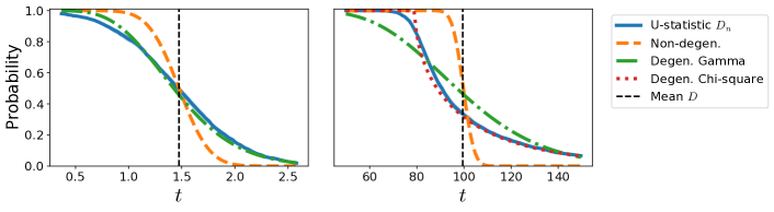
Figure 1: Behaviour of $\mathbb{P}(X>t)$ for $X=D_{n}$, a non-degenerate U-statistic, versus $X$ being different theoretical limits. Left. KSD with RBF kernel, $n=50$ and $d=2000$. Right. MMD with linear kernel, $n=50$ and $d=1000$. The left plot shows that $\mathbb{P}(D_{n}>t)$ disagrees with the non-degenerate limit from known classical results but aligns with the degenerate limit from ours (moment-matched by a Gamma variable – discussed in Section 3.2). The right plot is when the limit predicted by our result can be computed exactly as a shifted-and-rescaled chi-square and shows asymmetry, which confirms a departure from Gaussianity. See the last paragraph of Section 4.3 and Appendix A for simulation details.

In this paper, we prove a general convergence theorem for U-statistics of degree two, which holds in the high-dimensional setting and under very mild assumptions on the data. We observe a high-dimensional analogue of the classical behaviour: Depending on a moment ratio, the limiting distribution of U-statistics can take either the non-degenerate Gaussian limit, the degenerate limit or an intermediate distribution. Crucially, this happens regardless of the statistic’s degeneracy, as defined in the classical sense. We provide error bounds that are finite-sample valid and dimension-independent under a mild assumption.

In the context of kernel-based distribution tests, we show that our results hold for Maximum Mean Discrepancy (MMD) and for (Langevin) Kernelized Stein Discrepancy (KSD) under some natural conditions. We investigate several examples under Gaussian mean-shift – a setting purposely chosen to be as simple as possible to obtain good intuitions, while already capturing a rich amount of complex behaviours. Our theory correctly predicts the high-dimensional behaviour of the test power with a wider variance than classical results and, perhaps surprisingly, potential asymmetry (see Fig. 1 for one such example). Our results enable us to characterise such behaviours based on the size of $d$ and hyperparameter choices.

1.1 Overview of results

Given some i.i.d. data $\{\mathbf{X}_{i}\}_{i=1}^{n}$ drawn from a distribution $R$ on $\mathbb{R}^{d}$ and a symmetric measurable function $u:\mathbb{R}^{d}\times\mathbb{R}^{d}\rightarrow\mathbb{R}$, the goal is to estimate the quantity $D\coloneqq\mathbb{E}[u(\mathbf{X}_{1},\mathbf{X}_{2})]$. The U-statistic provides an unbiased estimator, defined as

Our main result is Theorem 3.2. Loosely speaking, it says that as $n,d\rightarrow\infty$, the statistic $D_{n}$ converges in distribution to a quadratic form of Gaussians:

$$D_{n}\;\xrightarrow{d}\;W+Z+D\;,$$ (2)

where $W$ is some infinite sum of weighted and centred chi-squares and $Z$ is some Gaussian. Define

$$\rho_{d}\coloneqq\sigma_{\rm full}\,/\,\sigma_{\rm cond}\;,\text{ where }\sigma_{\rm full}\;=\;\sqrt{\text{\rm Var}[u(\mathbf{X}_{1},\mathbf{X}_{2})]}\;\;\text{ and }\;\;\sigma_{\rm cond}\;=\;\sqrt{\text{\rm Var}\mathbb{E}[u(\mathbf{X}_{1},\mathbf{X}_{2})|\mathbf{X}_{1}]}\;,$$

and recall that the classical notion of degeneracy is defined by $\sigma_{\rm cond}=0$. We next observe that in (2), $W+D$ is closely related to the classical degenerate limit, whereas $Z+D$ gives exactly the classical non-degenerate limit. It turns out that, up to a mild assumption, the type of asymptotic distribution of $D_{n}$ is completely determined by the ratio $\rho_{d}$. This is reminiscent of the classical result, where the notion of degeneracy, i.e. whether $\sigma_{\rm cond}=0$, determines the limit of $D_{n}$. The difference in high dimensions is that $\sigma_{\rm full}$ and $\sigma_{\rm cond}$ may scale differently with $d$. Even if $\sigma_{\rm cond}\neq 0$, $\rho_{d}$ can grow to infinity as $d$ grows, causing a non-degenerate $D_{n}$ to behave like a degenerate U-statistic. We show that, depending on $\rho_{d}$, (2) becomes

$$D_{n}\;\xrightarrow{d} \;W+D\;\;\;\text{ for }\rho_{d}=\omega(n^{1/2})\; D_{n}\;\xrightarrow{d} \;Z+D\;\;\;\text{ for }\rho_{d}=o(n^{1/2})\;.$$ and

The second result is the classical Berry-Esséen bound for U-statistics, while the first result is new. It recovers the classical degenerate limit as a special case but also applies to very general U-statistics in high dimensions regardless of degeneracy.

The paper is organised as follows. Section 2 provides definitions and a sketch-of-intuition on the role of moment terms in the limiting behaviour of $D_{n}$. Section 3 presents the main results along with a proof overview in Section 3.3. Section 4.2 shows that these results apply to MMD and KSD under some natural conditions and Section 4.3 studies the Gaussian mean-shift case in detail.

1.2 Related literature

Convergence results for U-statistics. Existing high-dimensional results focus either on a different setting or on showing asymptotic normality under very specific assumptions on data; some references are provided at the start of this section. The results that resemble our work more closely are finite-sample bounds for classical degenerate U-statistics. Those works focus on providing bounds under conditions on specific eigenvalues of a spectral decomposition of $D_{n}$, and we defer a list of references to Remark 3.1. Among them, Yanushkevichiene (2012) provides a rate $O(n^{-1/12})$ under perhaps the least stringent assumption on eigenvalues, but the error is still pre-multiplied by the inverse square-root of the largest eigenvalue. These eigenvalues are intractable and yet depend on $d$ through the data distribution, which make them hard to apply to high-dimensional settings. In the classical setting where $d$ is fixed, a recent work by Bhattacharya et al. (2022) proves a Gaussian-quadratic-form limit similar to ours for a random quadratic polynomial, which includes a simple U-statistic as a special case. However, their results are asymptotic and in particular do not identify a parameter that leads to the phase transition. Our finite-sample results require a very different proof technique and show how a moment ratio governs the transition.

High-dimensional power analysis for MMD and KSD. Some recent work has investigated the asymptotic behaviour of $D_{n}$ for MMD. Yan and Zhang (2022) prove a convergence result under a specific data model and kernel choice, so that $u(\mathbf{x},\mathbf{y})=g(\|\mathbf{x}-\mathbf{y}\|_{2})$ for some function $g:\mathbb{R}\rightarrow\mathbb{R}$ and $\|{\,\vbox{\hbox{\tiny$\bullet$}}\,}\|_{2}$ being the vector norm. The dimension-independence of $g$ enables a Taylor expansion argument reminiscent of delta method and therefore gives a Gaussian limit. Such structures are not assumed in our work. A related work of Gao and Shao (2021) provides a finite-sample bound under more general conditions. The results show asymptotic normality of a studentised version of $D_{n}$ rather than $D_{n}$ itself, and the error bound is only valid if a moment ratio, analogous to excess kurtosis, vanishes with $d$ (see their Theorem 13). Interestingly, this effect is obtained as a special case of our results for much more general settings: In Section 3.2, we point out that the degenerate limit is Gaussian if and only if the excess kurtosis vanishes. Another recent line of work (Kim and Ramdas, 2020; Shekhar et al., 2022) focuses on a studentised $D_{n}$ that is modified to exclude half of the terms. They show dimension-agnostic normality results at the cost of not using the full U-statistic $D_{n}$.

2 Setup and motivation

We use the asymptotic notations $o,O,\Theta,\omega,\Omega$ defined in the usual way (see e.g. Chapter 3 of Cormen et al. (2009)) for the limit $n\rightarrow\infty$, where the dimension is allowed to depend on $n$; we make the $n$-dependence explicit in the dimension $d_{n}$ whenever such asymptotics are considered.

2.1 Moment terms in high dimensions

Consider a U-statistic $D_{n}$ as defined in (LABEL:eqn:general:u:defn) with respect to $(R,u)$ with mean $D=\mathbb{E}[u(\mathbf{X}_{1},\mathbf{X}_{2})]$. For $\nu\geq 1$, denote the $L_{\nu}$ norms by $\|{\,\vbox{\hbox{\tiny$\bullet$}}\,}\|_{L_{\nu}}\coloneqq\mathbb{E}[|{\,\vbox{\hbox{\tiny$\bullet$}}\,}|^{\nu}]^{1/\nu}$. The $\nu$-th central moment of $D_{n}$ are bounded from above and below in terms of two types of moment terms (see Lemma B.5 in the appendix):

$$M_{\rm cond;\nu}\coloneqq\big{\|}\mathbb{E}[u(\mathbf{X}_{1},\mathbf{X}_{2})|\mathbf{X}_{2}]-\mathbb{E}[u(\mathbf{X}_{1},\mathbf{X}_{2})]\big{\|}_{L_{\nu}},M_{\rm full;\nu}\coloneqq\big{\|}u(\mathbf{X}_{1},\mathbf{X}_{2})-\mathbb{E}[u(\mathbf{X}_{1},\mathbf{X}_{2})]\big{\|}_{L_{\nu}}.$$

In the special case $\nu=2$, the definitions from Section 1.1 implies $\sigma_{\rm cond}=M_{\rm cond;2}$, $\sigma_{\rm full}=M_{\rm full;2}$ and $\rho_{d}=\sigma_{\rm full}\,/\,\sigma_{\rm cond}$. The fact that these moments may scale with $d$ has a significant effect on convergence results: For example, bounds of the form $\frac{\rm moment}{f(n)}$ for some increasing function $f$ of $n$ are no longer guaranteed to be small. This is yet another effect of the “curse of dimensionality”. For U-statistics, the classical Berry-Esséen result (see e.g. Theorem 10.3 of Chen et al. (2011)) says that, if $\sigma_{\rm cond}>0$, then for a normal random variable $Z\sim\mathcal{N}(D,4n^{-1}\sigma_{\rm cond}^{2})$ and $\nu\in(2,3]$, we have

$$\sup\nolimits_{t\in\mathbb{R}}\Big{|}\mathbb{P}\Big{(}\mfrac{\sqrt{n}}{\sigma_{\rm cond}}D_{n}<t\Big{)}-\mathbb{P}\Big{(}\mfrac{\sqrt{n}}{\sigma_{\rm cond}}Z<t\Big{)}\Big{|}\;\leq\;\mfrac{6.1M_{\rm cond;\nu}^{\nu}}{n^{(\nu-2)/2}\sigma_{\rm cond}^{\nu}}+\mfrac{(1+\sqrt{2})\rho_{d}}{2(n-1)^{1/2}}\;.$$ (3)

Indeed, the error bound in the classical Berry-Esséen result is an increasing function of $n^{-1/2}\rho_{d}=\sigma_{\rm full}/(n^{1/2}\sigma_{\rm cond})$, which is not guaranteed to be small as $d$ grows.

The ratio $M_{\rm cond;\nu}/\sigma_{\rm cond}$ also appears in classical error bounds. However, we do not focus on how this ratio scales, since it appears in Berry-Esséen bounds even for sample averages. Error bounds in our main theorem will depend on similar ratios, and for our theorem to imply a convergence theorem, the following assumption is required:

Assumption 1

There exists some $\nu\in(2,3]$ and some constant $C<\infty$ such that for all $n$ and $d$, we have the uniform bounds $\frac{M_{\rm full;\nu}}{\sigma_{\rm full}}\leq C$ and $\frac{M_{\rm cond;\nu}}{\sigma_{\rm cond}}\leq C$ .

2.2 Sketch of intuition

We motivate our results by noting that the variance of $D_{n}$ defined in (LABEL:eqn:general:u:defn) satisfies

$$\text{\rm Var}[D_{n}]\;= \;O\Big{(}\mfrac{\mathbb{E}[(u(\mathbf{X}_{1},\mathbf{X}_{2})-D)(u(\mathbf{X}_{1},\mathbf{X}_{3})-D)]}{n}+\mfrac{\mathbb{E}[(u(\mathbf{X}_{1},\mathbf{X}_{2})-D)(u(\mathbf{X}_{1},\mathbf{X}_{2})-D)]}{n(n-1)}\Big{)}$$

$$\;= \;O\big{(}\mfrac{\sigma_{\rm cond}^{2}}{n}+\mfrac{\sigma_{\rm full}^{2}}{n(n-1)}\big{)}\;.$$

To study the asymptotic distribution of $D_{n}$, we need to understand how its asymptotic variance behaves as $n$ and $d$ grow. Suppose we are in the classical non-degenerate setting, where $d$ is fixed and $\sigma_{\rm cond}>0$. The dominating term in $\text{\rm Var}[D_{n}]$ is $O(n^{-1}\sigma_{\rm cond}^{2})$. The contribution of the $\sigma_{\rm full}^{2}$ term is small, i.e. the effect of the variance of each individual summand $u(\mathbf{X}_{1},\mathbf{X}_{2})$ is negligible. In fact, we can approximate $D_{n}$ by replacing each argument in the summand by an independent copy $\mathbf{X}^{\prime}_{i}$ of $\mathbf{X}_{i}$ and applying CLT for an empirical average:

$$D_{n}\;= \;D+\mfrac{1}{n(n-1)}\operatorname{\medmath\sum}_{1\leq i\neq j\leq n}(u(\mathbf{X}_{i},\mathbf{X}_{j})-D)$$

$$\;\approx \;D+\mfrac{1}{n}\operatorname{\medmath\sum}_{i=1}^{n}\Big{(}\mfrac{1}{n-1}\operatorname{\medmath\sum}_{j\neq i}(u(\mathbf{X}_{i},\mathbf{X}^{\prime}_{j})-D)\Big{)}+\mfrac{1}{n}\operatorname{\medmath\sum}_{j=1}^{n}\Big{(}\mfrac{1}{n-1}\operatorname{\medmath\sum}_{i\neq j}(u(\mathbf{X}^{\prime}_{i},\mathbf{X}_{j})-D)\Big{)}$$

$$\;= \;D+\mfrac{2}{n}\operatorname{\medmath\sum}_{i=1}^{n}\big{(}\mathbb{E}[u(\mathbf{X}_{i},\mathbf{X}^{\prime}_{j})|\mathbf{X}_{i}]-D\big{)}\;\approx\;\mathcal{N}\big{(}D\,,\,\mfrac{4\sigma_{\rm cond}^{2}}{n}\big{)}\;.$$

This argument underpins results on CLT for non-degenerate U-statistics. In the classical degenerate setting, however, $d$ is still fixed but $\sigma_{\rm cond}=0$, and the above argument fails to apply. Instead, one considers a spectral decomposition $u(\mathbf{x},\mathbf{y})=\sum_{k=1}^{\infty}\lambda_{k}\phi_{k}(\mathbf{x})\phi_{k}(\mathbf{y})$ for some eigenvalues $\{\lambda_{k}\}_{k=1}^{\infty}$ and eigenfunctions $\{\phi_{k}\}_{k=1}^{\infty}$, and compares the distribution of $D_{n}$ to a weighted sum of chi-squares:

$$D_{n}\;= \;\mfrac{1}{n(n-1)}\operatorname{\medmath\sum}_{1\leq i\neq j\leq n}\operatorname{\medmath\sum}_{k=1}^{\infty}\lambda_{k}\phi_{k}(\mathbf{X}_{i})\phi_{k}(\mathbf{X}_{j})$$

$$\;= \;\operatorname{\medmath\sum}_{k=1}^{\infty}\lambda_{k}\Big{(}\Big{(}\mfrac{1}{n}\operatorname{\medmath\sum}_{i=1}^{n}\phi_{k}(\mathbf{X}_{i})\Big{)}\Big{(}\mfrac{1}{n}\operatorname{\medmath\sum}_{j=1}^{n}\phi_{k}(\mathbf{X}_{j})\Big{)}-\mfrac{1}{n^{2}}\operatorname{\medmath\sum}_{i=1}^{n}\phi_{k}(\mathbf{X}_{i})^{2}\Big{)}$$

$$\;\approx \;\mfrac{1}{n}\operatorname{\medmath\sum}_{k=1}^{\infty}\lambda_{k}\,\big{(}\big{(}\sqrt{\text{\rm Var}[\phi_{k}(\mathbf{X}_{1})]}\,\xi_{k}+\mathbb{E}[\phi_{k}(\mathbf{X}_{1})]\big{)}^{2}-\mathbb{E}[\phi_{k}(\mathbf{X}_{1})^{2}]\big{)}\;,$$

where $\xi_{k}$’s are i.i.d. standard normals. The limiting distributions in both settings enable one to construct consistent confidence intervals for $D_{n}$ and study $\mathbb{P}(D_{n}>t)$.

The key takeaway is that the asymptotic distribution of $D_{n}$ depends on the relative sizes of $\sigma_{\rm cond}^{2}$ and $(n-1)^{-1}\sigma_{\rm full}^{2}$. This comparison reduces to degeneracy when $d$ is fixed, but is no longer so when $d$ grows. In the high-dimensional setting, $\sigma_{\rm cond}$ and $\sigma_{\rm full}$ can scale with $d$ at different orders, making it possible for the ratio $\rho_{d}$ to vary with $d$. In particular, a non-degenerate U-statistic with $\sigma_{\rm cond}>0$ may still satisfy $\rho_{d}=\omega(n^{1/2})$, i.e. $(n-1)^{-1}\sigma_{\rm full}^{2}/\sigma_{\rm cond}^{2}\rightarrow\infty$ as $n$ and $d$ grow. In this case, the classical argument for a non-degenerate Gaussian limit would fail and a degenerate limit would dominate. This is exactly what we observe in the practical applications in Section 4.3, and motivates the need for results that explicitly addresses the high-dimensional setting.

3 Main results

The main result presented in this section is a finite-sample bound that compares $D_{n}$ to a quadratic form of infinitely many Gaussians. The limiting distribution is a sum of the non-degenerate limit and a variant of the degenerate limit, and subject to 1, the error bound is independent of $\rho_{d}$. In the case $\rho_{d}=o(n^{1/2})$, the non-degenerate limit dominates and our result agrees with the Gaussian limit given by a Berry-Esséen theorem for U-statistics. However when dimension is high such that $\rho_{d}=\omega(n^{1/2})$, the degenerate limit dominates and implies a larger asymptotic variance. We also discuss how to obtain consistent distribution bounds that reflect the effect of a large dimension $d$ on the original statistic $D_{n}$.

Our results rest on a functional decomposition assumption. For a sequence of $\mathbb{R}^{d}\rightarrow\mathbb{R}$ functions $\{\phi_{k}\}_{k=1}^{\infty}$ and a sequence of real values $\{\lambda_{k}\}_{k=1}^{\infty}$, we define the $L_{\nu}$ approximation error for $\nu\geq 1$ and a given $K\in\mathbb{N}$ as

$$\varepsilon_{K;\nu}\;\coloneqq\;\big{\|}\operatorname{\medmath\sum}_{k=1}^{K}\lambda_{k}\phi_{k}(\mathbf{X}_{1})\phi_{k}(\mathbf{X}_{2})-u(\mathbf{X}_{1},\mathbf{X}_{2})\big{\|}_{L_{\nu}}\;.$$

Assumption 2

There exists some $\nu\in(2,3]$ such that, for any fixed $n$ and $d$, as $K\rightarrow\infty$, the $L_{\nu}$ approximation error $\varepsilon_{K;\nu}\rightarrow 0$ for some choice of $\{\phi_{k}\}_{k=1}^{\infty}$ and $\{\lambda_{k}\}_{k=1}^{\infty}$.

Remark 3.1.

(i) If 2 holds for some $\nu>3$, it certainly holds for $\nu=3$. We restrict our focus to $\nu\in(2,3]$ for simplicity. (ii) 2 always holds for $\nu=2$ by the spectral decomposition of an operator on $L_{2}(\mathbb{R}^{d},R)$. For degenerate U-statistics with $d$ fixed, the corresopnding orthonormal eigenbasis of functions and eigenvalues are used to prove asymptotic results (see Section 5.5.2 of Serfling (1980)) and finite-sample bounds (Bentkus and Götze, 1999; Götze and Tikhomirov, 2005; Yanushkevichiene, 2012). In fact, these finite-sample bounds are dependent on the specific $\lambda_{k}$’s, making the results hard to apply. Instead, we forgo orthonormality at the cost of a convergence slightly stronger than $L_{2}$. This allows for a much more flexible choice of $\{\phi_{k},\lambda_{k}\}_{k=1}^{\infty}$ and is particularly well-suited for a kernel-based setting; see Remark 4.4 for a discussion.

Before stating the results, we introduce some more notations. For every $K\in\mathbb{N}$, we define a diagonal matrix of the first $K$ “eigenvalues” and a concatenation of the first $K$ “eigenfunctions” by

$$\Lambda^{K}\;\coloneqq\;\text{\rm diag}\{\lambda_{1},\ldots,\lambda_{K}\}\;\in\mathbb{R}^{K\times K}\;, \phi^{K}(x)\;\coloneqq\;(\phi_{1}(x),\ldots,\phi_{K}(x))^{\top}\;\in\mathbb{R}^{K}\;.$$ (4)

We denote the mean and variance of $\phi^{K}(\mathbf{X}_{1})$ by $\mu^{K}\coloneqq\mathbb{E}[\phi^{K}(\mathbf{X}_{1})]$ and $\Sigma^{K}\coloneqq\text{\rm Cov}[\phi^{K}(\mathbf{X}_{1})]$.

3.1 Result for the general case

Let $\eta^{K}_{i}$, with $i,K\in\mathbb{N}$, be i.i.d. standard Gaussian vectors in $\mathbb{R}^{K}$. In the general case, the limiting distribution is given in terms of a quadratic form of Gaussians, defined by

$$U^{K}_{n}\coloneqq\mfrac{1}{n(n-1)}\operatorname{\medmath\sum}_{1\leq i\neq j\leq n}(\eta^{K}_{i})^{\top}(\Sigma^{K})^{1/2}\Lambda^{K}(\Sigma^{K})^{1/2}\eta^{K}_{j}+\mfrac{2}{n}\operatorname{\medmath\sum}_{i=1}^{n}(\mu^{K})^{\top}\Lambda^{K}(\Sigma^{K})^{1/2}\eta^{K}_{i}+D.$$

We also denote the dominating moment terms by

$$\sigma_{\rm max}\;\coloneqq\;\max\{\sigma_{\rm full},(n-1)^{1/2}\sigma_{\rm cond}\}\;, M_{\rm max;\nu}\;\coloneqq\;\max\{M_{\rm full;\nu},(n-1)^{1/2}M_{\rm cond;\nu}\}\;.$$

We are ready to state our main result – a finite-sample error bound that compares $D_{n}$ to the limiting distribution of $U_{n}^{K}$, where the error is given in terms of $n$ and the moment terms.

Theorem 3.2.

There exists a constant $C>0$ such that, for all $u$, $R$, $d$ and $n$, if $\nu\in(2,3]$ satisfies 2, then the following holds:

$$\sup\nolimits_{t\in\mathbb{R}}\Big{|}\mathbb{P}\Big{(} \mfrac{\sqrt{n(n-1)}}{\sigma_{\rm max}}D_{n}>t\Big{)}-\lim_{K\rightarrow\infty}\mathbb{P}\Big{(}\mfrac{\sqrt{n(n-1)}}{\sigma_{\rm max}}U_{n}^{K}>t\Big{)}\Big{|}$$

$$\;\leq \;C\,n^{-\frac{\nu-2}{4\nu+2}}\Big{(}\mfrac{(M_{\rm full;\nu})^{\nu}}{\sigma_{\rm max}^{\nu}}+\mfrac{((n-1)^{1/2}\,M_{\rm cond;\nu})^{\nu}}{\,\sigma_{\rm max}^{\nu}}\Big{)}^{\frac{1}{2\nu+1}}\;\leq\;2^{\frac{1}{2\nu+1}}C\,n^{-\frac{\nu-2}{4\nu+2}}\Big{(}\mfrac{M_{\rm max;\nu}}{\sigma_{\rm max}}\Big{)}^{\frac{\nu}{2\nu+1}}\;.$$

Remark 3.3.

If $\nu=3$, the RHS is given by $2^{3/7}Cn^{-\frac{1}{14}}\big{(}\frac{M_{\rm max;3}}{\sigma_{\rm max}}\big{)}^{6/7}$. If 1 holds for $\nu$, the RHS can be replaced by $C^{\prime}n^{-\frac{\nu-2}{4\nu+2}}$ for some constant $C^{\prime}$ and is dimension-independent.

Remark 3.4.

At first sight, one may be tempted to move $\lim_{K\rightarrow\infty}$ inside $\mathbb{P}$ such that, instead of the cumbersome expression of $W_{n}^{K}$ with finite $K$, one may deal with random quantities in a Hilbert space. The reason to stick with $W_{n}^{K}$ is that in 2, convergence of the infinite sum is required only in $L_{\nu}$ and not almost surely. This makes verification of the assumption substantially simpler in practice: In Appendix A, we illustrate how this assumption holds via a simple Taylor-expansion argument coupled with suitable tail behaviour of the data to control error terms. The same argument is not applicable if we instead require an almost sure convergence.

Theorem 3.2 immediately implies a convergence theorem:

Corollary 3.5.

Let the dimension $d_{n}$ depend on $n$. Suppose Assumptions 1 and 2 hold for some $\nu>2$ and the sequential distribution limit $\bar{U}=\lim_{n\rightarrow\infty}\lim_{K\rightarrow\infty}\frac{\sqrt{n(n-1)}}{\sigma_{\rm max}}(U_{n}^{K}-D)$ exists. Then

$$\mfrac{\sqrt{n(n-1)}}{\sigma_{\rm max}}(D_{n}-D)\xrightarrow{d}\bar{U} \;\text{ as }\;n\rightarrow\infty\;.$$

$U_{n}^{K}$ is a quadratic form of Gaussians, which does not admit a closed-form c.d.f. in general and whose limiting behaviour depends heavily on $\lambda_{k}$ and $\phi_{k}$. Nevertheless, the presence of Gaussianity still allows us to obtain crude bounds that reflect how dimension $d$ affects its distribution. By combining such bounds with Theorem 3.2, we can bound the c.d.f. of the original U-statistic $D_{n}$.

Proposition 3.6.

There exists constants $C_{1},C_{2},C_{3}>0$ such that, for all $u$, $R$, $d$, $n$ and $K$, if $\nu\in(2,3]$ satisfies 2, then for all $\epsilon>0$,

$$\mathbb{P}(|D_{n}-D|>\epsilon)\;\geq \;\;1-C_{1}\Big{(}\mfrac{\sqrt{n(n-1)}}{\sigma_{\rm max}}\Big{)}^{1/2}\epsilon^{1/2}-C_{2}\,n^{-\frac{\nu-2}{4\nu+2}}\Big{(}\mfrac{M_{\rm max;\nu}}{\sigma_{\rm max}}\Big{)}^{\frac{\nu}{2\nu+1}}\;,$$

$$\mathbb{P}(|D_{n}-D|>\epsilon)\;\leq \;\;C_{3}\epsilon^{-2}\Big{(}\mfrac{\sigma_{\rm max}}{\sqrt{n(n-1)}}\Big{)}^{2}\;.$$

Remark 3.7.

The second bound is a concentration inequality directly available via Markov’s inequality, whereas the first bound is an anti-concentration result. Anti-concentration results are generally available only for random variables from known distribution families, and we obtain such a result by comparing $D_{n}$ to $U^{K}_{n}$. The error bounds are free of any dependence on $K$ and specific choices of $\phi_{k}$ and $\lambda_{k}$. The trailing error term involving $M_{\rm max;\nu}/\sigma_{\rm max}$ is inherited from Theorem 3.2 and is negligible, whereas the other error term is directly related to the inverse of the Markov error term.

Proposition 3.6 provide two-sided bounds on how likely it is for $D_{n}$ to be far from $D$. The next corollary provides a more explicit statement.

Corollary 3.8.

Let the dimension $d_{n}$ depend on $n$ and fix $\epsilon>0$. Suppose Assumptions 1 and 2 hold for some $\nu\in(2,3]$. As $n\rightarrow\infty$, we have that $\mathbb{P}(|D_{n}-D|>\epsilon)\rightarrow 1$  if  $\sigma_{\rm max}=\omega(n)$ and $\mathbb{P}(|D_{n}-D|>\epsilon)\rightarrow 0$  if  $\sigma_{\rm max}=o(n)$.

Another way of formulating the bounds in Proposition 3.6 is the following: Similar to the intuition for a Gaussian, when $n$ is large (with $d_{n}$ depending on $n$), the distribution of $D_{n}$ is not only concentrated in an interval around $D$ with width being a multiple of $\frac{\sigma_{\rm max}}{n}$, but also “well spread-out” within the interval. The probability mass gets concentrated around $D$ when $\sigma_{\rm max}=o(n)$, but spreads out along the whole real line when $\sigma_{\rm max}=\omega(n)$; the latter only happens in a high dimensional regime.

To have a more precise understanding of the limiting behaviour of $D_{n}$, we need a better knowledge of $U_{n}^{K}$. By a closer examination of $U_{n}^{K}$, we see that it is a sum of three terms: A sum of weighted chi-squares with variance of the order $n^{-1}(n-1)^{-1}\sigma_{\rm full}^{2}$, a Gaussian with variance of the order $n^{-1}\sigma_{\rm cond}^{2}$, and a constant $D$. The first term closely resembles the limit for degenerate U-statistics when $d$ is fixed, while the second term corresponds exactly to the Gaussian limit for non-degenerate U-statistics. It turns out that, unless we are at the boundary case where $\rho_{d}=\Theta(n^{1/2})$, we can always approximate $U_{n}^{K}$ by ignoring either the first or the second term. Ignoring the first term gives exactly the Gaussian limit, where a well-established result has already been provided in (3). Ignoring the second term gives an infinite sum of weighted chi-squares, which is discussed next.

3.2 The case $\rho_{d}=\omega(n^{1/2})$

Let $\{\xi_{k}\}_{k=1}^{\infty}$ be a sequence of i.i.d. standard Gaussians in 1d, and for $K\in\mathbb{N}$, let $\{\tau_{k;d}\}_{k=1}^{K}$ be the eigenvalues of $(\Sigma^{K})^{1/2}\Lambda^{K}(\Sigma^{K})^{1/2}$. The limiting distribution we consider is given in terms of

$$W_{n}^{K}\;\coloneqq\;\mfrac{1}{\sqrt{n(n-1)}}\operatorname{\medmath\sum}_{k=1}^{K}\tau_{k;d}(\xi_{k}^{2}-1)+D\;.$$ (5)

Note that in this case, $\sigma_{\rm max}=\sigma_{\rm full}$. The next result adapts Theorem 3.2 by replacing $U_{n}^{K}$ with $W_{n}^{K}$:

Proposition 3.9.

There exists a constant $C>0$ such that, for all $u$, $R$, $d$, $n$ and $K$, if $\nu\in(2,3]$ satisfies 2, then the following holds:

$$\sup\nolimits_{t\in\mathbb{R}} \Big{|}\mathbb{P}\Big{(}\mfrac{\sqrt{n(n-1)}}{\sigma_{\rm full}}D_{n}>t\Big{)}-\lim_{K\rightarrow\infty}\mathbb{P}\Big{(}\mfrac{\sqrt{n(n-1)}}{\sigma_{\rm full}}W_{n}^{K}>t\Big{)}\Big{|}$$

$$\leq\;C\Big{(}\mfrac{1}{(n-1)^{1/5}}+\Big{(}\mfrac{\sqrt{n-1}\,\sigma_{\rm cond}}{\sigma_{\rm full}}\Big{)}^{2/5}+\,n^{-\frac{\nu-2}{4\nu+2}}\Big{(}\mfrac{(M_{\rm full;\nu})^{\nu}}{\sigma_{\rm full}^{\nu}}+\mfrac{((n-1)^{1/2}M_{\rm cond;\nu})^{\nu}}{\sigma_{\rm full}^{\nu}}\Big{)}^{\frac{1}{2\nu+1}}\Big{)}\;.$$

Remark 3.10.

In the case $\nu=3$, the error term above becomes

$$C\Big{(}\mfrac{1}{(n-1)^{1/5}}+\Big{(}\mfrac{\sqrt{n-1}\,\sigma_{\rm cond}}{\sigma_{\rm full}}\Big{)}^{2/5}+\,n^{-\frac{1}{14}}\Big{(}\mfrac{(M_{\rm full;3})^{3}}{\sigma_{\rm full}^{3}}+\mfrac{\big{(}(n-1)^{1/2}M_{\rm cond;3}\big{)}^{3}}{\sigma_{\rm full}^{3}}\Big{)}^{\frac{1}{7}}\Big{)}\;.$$

In the case when 1 holds for $\nu$, the error term is $\Theta\big{(}\big{(}\frac{n-1}{\rho_{d}^{2}}\big{)}^{1/5}+n^{-\frac{\nu-2}{4\nu+2}}\big{)}$.

Remark 3.11.

Proposition 3.9 agrees with the classical results for degenerate U-statistics. In those results, $\{\phi_{k}\}_{k=1}^{\infty}$ are chosen such that they are orthonormal in $L_{2}(\mathbb{R}^{d},R)$ and $\mathbb{E}[\phi_{k}(\mathbf{X}_{1})]=0$. This corresponds to $\Sigma^{K}$ being a diagonal matrix and the expression for $\tau_{k;d}$ can be simplified.

We seek to obtain a better understanding of the limiting distribution of $D_{n}$ in the case $\rho_{d}=\omega(n^{1/2})$. Write $W_{n}\coloneqq\lim_{K\rightarrow\infty}W_{n}^{K}$ as the distributional limit of $W_{n}^{K}$ as $K\rightarrow\infty$. Provided that $W_{n}$ exists, Proposition 3.9 gives the convergence of $D_{n}$ to $W_{n}$ in the Kolmogorov metric. The next lemma guarantees the existence of $W_{n}$.

Proposition 3.12.

Fix $n,d$. If 2 holds for some $\nu\geq 2$ and $|D|,\sigma_{\rm full}<\infty$, $W_{n}$ exists.

While $W_{n}^{K}$ is a sum of chi-squares, the distributional limit $W_{\infty}\coloneqq\lim_{n\rightarrow\infty}\lim_{K\rightarrow\infty}W_{n}^{K}$ may actually be Gaussian. The crucial subtlety lies in the fact that the weights of $W_{n}^{K}$ may depend on $K$ and also on $n$ (through $d\equiv d_{n}$). In what is well-known in the probability literature as the “fourth moment phenomenon” (Nualart and Peccati, 2005), the necessary and sufficient condition for Gaussianity of $W_{\infty}$ is that the limiting excess kurtosis is zero. In our case, the limiting moments can be computed easily when 2 holds for $\nu\geq 4$, as they depend only on moments of the original function $u$ and not on specific values of the intractable weights $\tau_{k;d}$. Lemma B.8 in the appendix shows that $\mathbb{E}[W_{n}^{K}]=D$ for every $K\in\mathbb{N}$,   $\lim_{K\rightarrow\infty}\text{\rm Var}[W_{n}^{K}]=\frac{2}{n(n-1)}\sigma_{\rm full}^{2}$ and

$$\lim_{K\rightarrow\infty}\mathbb{E}\big{[}(W_{n}^{K}-D)^{4}\big{]}\;=\;\mfrac{12(4\mathbb{E}[u(\mathbf{X}_{1},\mathbf{X}_{2})u(\mathbf{X}_{2},\mathbf{X}_{3})u(\mathbf{X}_{3},\mathbf{X}_{4})u(\mathbf{X}_{4},\mathbf{X}_{1})]+\sigma_{\rm full}^{4})}{n^{2}(n-1)^{2}}\;,$$

provided that 2 holds for $\nu\geq 1$, $\nu\geq 2$ and $\nu\geq 4$ respectively. If the excess kurtosis is indeed zero, Gaussian is still the correct limiting distribution for $D_{n}$, but now with a larger variance (characterized by $\sigma_{\rm full}$) than the one naively predicted by the Gaussian CLT limit for non-degenerate U-statistics. Meanwhile, when the excess kurtosis is not zero, the limiting distribution is an infinite sum of weighted chi-squares. A naive example is the following:

Lemma 3.13.

Suppose there exists a finite $K_{*}$ such that $\lambda_{k}=0$ for all $k>K_{*}$. Then $W_{n}=W_{n}^{K^{*}}$, which is a weighted sum of chi-squares.

A weighted sum of chi-squares does not admit a closed-form distribution function. Fortunately in the case when $\tau_{k;d}\geq 0$ for all $k$, many numerical approximation schemes are available and used widely. These methods generally rely on matching the moments of $W_{n}$, which can be computed easily due to Proposition 3.12. The simplest example is the Welch-Satterthwaite method, which approximates the distribution of $W_{n}$ by a gamma distribution with the same mean and variance. We refer readers to Bodenham and Adams (2016) and Duchesne and De Micheaux (2010) for a review of other moment-matching methods.

3.3 Proof overview

The proof for Theorem 3.2 consists of three main steps:

1. “Spectral” approximation. We first use 2 to replace $u(\mathbf{X}_{i},\mathbf{X}_{j})$ with the truncated sum $\sum_{k=1}^{K}\lambda_{k}\phi_{k}(\mathbf{X}_{i})\phi_{k}(\mathbf{X}_{j})$, which gives a truncation error that vanishes as $K\rightarrow\infty$;

2. Gaussian approximation. The truncated sum is a simple quadratic form of i.i.d. vectors in $\mathbb{R}^{d}$, each of which can be approximated by a Gaussian vector. This is done by following Chatterjee (2006)’s adaptataion of Lindeberg’s telescoping sum argument. Similar proof ideas have been used to develop new convergence results in statistics and machine learning; examples include empirical risk (Montanari and Saeed, 2022) and bootstrap for non-asymptotically normal estimators (Austern and Syrgkanis, 2020). This step introduces errors in terms of moment terms of $U_{n}^{K}$, which are then related to those of $D_{n}$;

3. Bound the distribution of $U_{n}^{K}$. Step (ii) introduces errors in terms of the distribution of $U_{n}^{K}$, a quadratic form of Gaussians, over a short interval. These errors are then controlled by the distribution bounds from Carbery and Wright (2001).

The proof for Proposition 3.9 is similar, except that we use an additional Markov-type argument to remove the linear sum from $U_{n}^{K}$ and obtain the limit in terms of $W_{n}^{K}$.

4 Kernel-based testing in high dimensions

Given two probability measures $P$ and $Q$ on $\mathbb{R}^{d}$, we consider the problem of testing $H_{0}:P=Q$ against $H_{1}:P\neq Q$ through some measure of discrepancy between $P$ and $Q$. We focus on Maximum Mean Discrepancy (MMD) and (Langevin) Kernelized Stein Discrepancy (KSD), two kernel-based methods that use a U-statistic $D_{n}$ as the test statistic. It is well-known that $\sigma_{\rm cond}=0$ under $H_{0}$ and the limit of $D_{n}$ is a weighted sum of chi-squares (see Gretton et al. (2012) for MMD and Liu et al. (2016) for KSD). Instead, we are interested in quantifying the power of $D_{n}$ given as $\mathbb{P}_{H_{1}}(D_{n}>t)$. The test threshold $t$ is often chosen adaptively in practice, but we assume $t$ to be fixed for simplicity of analysis. The results in Section 3 offer two key insights to this problem:

1. $D_{n}$ may have different limiting distributions depending on $\rho_{d}$. In the non-Gaussian case, the confidence interval and thereby the distribution curve can be wider than what a Berry-Esséen bound predicts, and there may be potential asymmetry;

2. We can completely characterise the high-dimensional behaviour of the power in terms of $\rho_{d}$, which in turn depends on the hyperparameters and the set of alternatives considered.

In this section, we first show that our results naturally apply to MMD and KSD. We then investigate their high-dimensional behaviours in an example of Gaussian mean-shift under simple kernels. Throughout, $\|{\,\vbox{\hbox{\tiny$\bullet$}}\,}\|_{2}$ denotes the vector Euclidean norm, which is not to be confused with $\|{\,\vbox{\hbox{\tiny$\bullet$}}\,}\|_{L_{2}}$.

4.1 Notations

We follow the kernel definition from Steinwart and Scovel (2012) as below:

Definition 4.1.

A function $\kappa:\mathbb{R}^{d}\times\mathbb{R}^{d}\rightarrow\mathbb{R}$ is called a kernel on $\mathbb{R}^{d}$ if there exists a Hilbert space $(\mathcal{H},\langle{\,\vbox{\hbox{\tiny$\bullet$}}\,},{\,\vbox{\hbox{\tiny$\bullet$}}\,}\rangle_{\mathcal{H}})$ and a map $\phi:\mathbb{R}^{d}\rightarrow\mathcal{H}$ such that $\kappa(\mathbf{x},\mathbf{x}^{\prime})=\langle\phi(\mathbf{x}),\phi(\mathbf{x}^{\prime})\rangle_{\mathcal{H}}$ for all $\mathbf{x},\mathbf{x}^{\prime}\in\mathcal{H}$.

We give the minimal definitions of MMD and KSD, and refer interested readers to Gretton et al. (2012) and Gorham and Mackey (2017) for further reading. Throughout, we let $\{\mathbf{Y}_{j}\}_{j=1}^{n}$ be i.i.d. samples from $P$ and $\{\mathbf{X}_{i}\}_{i=1}^{n}$ be i.i.d. samples from $Q$. We also write $\mathbf{Z}_{i}\coloneqq(\mathbf{X}_{i},\mathbf{Y}_{i})$ and assume that $\kappa$ is measurable. MMD with respect to $\kappa$ is defined by

$$D^{\rm MMD}(Q,P)\;\coloneqq\;\mathbb{E}_{\mathbf{Y},\mathbf{Y}^{\prime}\sim P}[\kappa(\mathbf{Y},\mathbf{Y}^{\prime})]-2\mathbb{E}_{\mathbf{Y}\sim P,\mathbf{X}\sim Q}[\kappa(\mathbf{Y},\mathbf{X})]+\mathbb{E}_{\mathbf{X},\mathbf{X}^{\prime}\sim Q}[\kappa(\mathbf{X},\mathbf{X}^{\prime})]\;.\vspace{-0.5em}$$

A popular unbiased estimator for $D^{\rm MMD}$ is exactly a U-statistic:

$$D^{\rm MMD}_{n}\;\coloneqq\;\mfrac{1}{n(n-1)}\operatorname{\medmath\sum}_{1\leq i\neq j\leq n}u^{\rm MMD}(\mathbf{Z}_{i},\mathbf{Z}_{j})\;,\vspace{-0.5em}$$

where the summand is given by $u^{\rm MMD}\big{(}(\mathbf{x},\mathbf{y}),(\mathbf{x}^{\prime},\mathbf{y}^{\prime})\big{)}\coloneqq\kappa(\mathbf{x},\mathbf{x}^{\prime})+\kappa(\mathbf{y},\mathbf{y}^{\prime})-\kappa(\mathbf{x},\mathbf{y}^{\prime})-\kappa(\mathbf{x}^{\prime},\mathbf{y})$. To define KSD, we assume that $\kappa$ is continuously differentiable with respect to both arguments, and $P$ admits a continuously differentiable, positive Lebesgue density $p$. The following formulation of KSD is due to Theorem 2.1 of Chwialkowski et al. (2016):

$$D^{\rm KSD}(Q,P)\;\coloneqq\;\mathbb{E}_{\mathbf{X},\mathbf{X}^{\prime}\sim Q}[u_{P}^{\rm KSD}(\mathbf{X},\mathbf{X}^{\prime})]\;,\vspace{-0.5em}$$

where we assume $\mathbb{E}_{\mathbf{X}\sim Q}[u_{P}^{\rm KSD}(\mathbf{X},\mathbf{X})]<\infty$ and the function $u_{P}^{\rm KSD}:\mathbb{R}^{d}\times\mathbb{R}^{d}\rightarrow\mathbb{R}$ is given by

$$u_{P}^{\rm KSD}(\mathbf{x},\mathbf{x}^{\prime})= \;\big{(}\nabla\log p(\mathbf{x})\big{)}^{\top}\big{(}\nabla\log p(\mathbf{x}^{\prime})\big{)}\kappa(\mathbf{x},\mathbf{x}^{\prime})\;+\;\big{(}\nabla\log p(\mathbf{x})\big{)}^{\top}\nabla_{2}\kappa(\mathbf{x},\mathbf{x}^{\prime})$$

$$+\big{(}\nabla\log p(\mathbf{x}^{\prime})\big{)}^{\top}\nabla_{1}\kappa(\mathbf{x},\mathbf{x}^{\prime})\;+\;\text{\rm Tr}(\nabla_{1}\nabla_{2}\kappa(\mathbf{x},\mathbf{x}^{\prime}))\;.$$

$\nabla_{1}$ and $\nabla_{2}$ are the differential operators with respect to the first and second arguments of $\kappa$ respectively. The estimator is again a U-statistic, given by $D^{\rm KSD}_{n}\coloneqq\frac{1}{n(n-1)}\sum_{1\leq i\neq j\leq n}u_{P}^{\rm KSD}(\mathbf{X}_{i},\mathbf{X}_{j})$.

4.2 General results

We show that a kernel structure allows 2 to be fulfilled under some natural conditions. Let $\mathbf{V}_{1},\mathbf{V}_{2}\overset{i.i.d.}{\sim}R$ for some probability measure $R$ on $\mathbb{R}^{b}$ and $\kappa^{*}$ be a measurable kernel on $\mathbb{R}^{b}$. A sequence of functions $\{\phi_{k}\}_{k=1}^{\infty}$ in $L_{2}(\mathbb{R}^{b},R)$ and a sequence of non-negative values $\{\lambda_{k}\}_{k=1}^{\infty}$ with $\lim_{k\rightarrow\infty}\lambda_{k}=0$ is called a weak Mercer representation if

$$\big{|}\operatorname{\medmath\sum}_{k=1}^{K}\lambda_{k}\phi_{k}(\mathbf{V}_{1})\phi_{k}(\mathbf{V}_{2})-\kappa^{*}(\mathbf{V}_{1},\mathbf{V}_{2})\big{|}\rightarrow 0\;\;\text{ almost surely }\;\;\qquad\text{ as }K\rightarrow\infty\;.$$

Steinwart and Scovel (2012) show that such a representation exists if $\mathbb{E}[\kappa^{*}(\mathbf{V}_{1},\mathbf{V}_{1})]<\infty$, whose result is summarised in Lemma B.12 in the appendix. To deduce from this the $L_{\nu}$ convergence of 2, we need the following assumptions on the kernel $\kappa^{*}$:

Assumption 3

Fix $\nu>2$. Assume $\mathbb{E}[\kappa^{*}(\mathbf{V}_{1},\mathbf{V}_{1})]<\infty$ and let $\{\lambda_{k}\}_{k=1}^{\infty}$ and $\{\phi_{k}\}_{k=1}^{\infty}$ be a weak Mercer representation of $\kappa^{*}$ under $R$. Also assume that for some $\nu^{*}>\nu$, $\|\kappa^{*}(\mathbf{V}_{1},\mathbf{V}_{2})\|_{L_{\nu^{*}}}<\infty$ and $\sup_{K\geq 1}\|\sum_{k=1}^{K}\lambda_{k}\phi_{k}(\mathbf{V}_{1})\phi_{k}(\mathbf{V}_{2})\|_{L_{\nu^{*}}}<\infty$ .

For MMD, we can use the weak Mercer representation of $u^{\rm MMD}$ to show that our results apply:

Lemma 4.2.

$u^{\rm MMD}$ defines a kernel on $\mathbb{R}^{2d}$. Moreover, if 3 holds for $\kappa^{*}=u^{\rm MMD}$ under $P\otimes Q$ for some $\nu>2$, then 2 holds for $\min\{\nu,3\}$ with $u=u^{\rm MMD}$ and $R=P\otimes Q$.

In the case of KSD, we use the representation of $\kappa$ directly. We require some additional assumptions for the score function $\nabla\log p(\mathbf{x})$ to be well-behaved and the differential operation on $\kappa$ to behave well under the representation.

Assumption 4

Fix $n$, $d$ and $\nu>2$. Assume that 3 holds with $\nu$ for $\kappa$ under $Q$, with $\{\lambda_{k}\}_{k=1}^{\infty}$ and $\{\phi_{k}\}_{k=1}^{\infty}$ as the weak Mercer representation of $\kappa$ under $Q$ and $\nu^{*}$ being defined as in 3. Further assume that (i) $\|\|\nabla\log p(\mathbf{X}_{1})\|_{2}\|_{L_{2\nu^{**}}}<\infty$ for $\nu^{**}=\frac{\nu(\nu+\nu^{*})}{\nu^{*}-\nu}$ ; (ii) $\sup_{k\in\mathbb{N}}\|\phi_{k}(\mathbf{X}_{1})\|_{L_{2\nu}}<\infty$; (iii) $\phi_{k}$’s are differentiable with $\sup_{k\in\mathbb{N}}\|\|\nabla\phi_{k}(\mathbf{X}_{1})\|_{2}\|_{L_{\nu}}<\infty$; (iv) As $K\rightarrow\infty$, we have the convergence $\big{\|}\big{\|}\sum_{k=1}^{K}\lambda_{k}(\nabla\phi_{k}(\mathbf{X}_{1}))\phi_{k}(\mathbf{X}_{2})-\nabla_{1}\kappa(\mathbf{X}_{1},\mathbf{X}_{2})\big{\|}_{2}\big{\|}_{L_{2\nu}}\rightarrow 0$ as well as the convergence $\big{\|}\sum_{k=1}^{K}\lambda_{k}(\nabla\phi_{k}(\mathbf{X}_{1}))^{\top}(\nabla\phi_{k}(\mathbf{X}_{2}))-\text{\rm Tr}(\nabla_{1}\nabla_{2}\kappa(\mathbf{X}_{1},\mathbf{X}_{2}))\big{\|}_{L_{\nu}}\rightarrow 0$.

We can now form a decomposition of $u_{P}^{\rm KSD}$. Given $\{\lambda_{k}\}_{k=1}^{\infty}$ and $\{\phi_{k}\}_{k=1}^{\infty}$ from 4 and any fixed $d\in\mathbb{N}$, define the sequences $\{\alpha_{k}\}_{k=1}^{\infty}$ and $\{\psi_{k}\}_{k=1}^{\infty}$ as, for $1\leq l\leq d$ and $k^{\prime}\in\mathbb{N}$,

$$\alpha_{(k^{\prime}-1)d+l}\;\coloneqq \;\lambda_{k^{\prime}}\; \psi_{(k^{\prime}-1)d+l}(\mathbf{x})\;\coloneqq \;(\partial_{x_{l}}\log p(\mathbf{x}))\phi_{k^{\prime}}(\mathbf{x})+\partial_{x_{l}}\phi_{k^{\prime}}(\mathbf{x})\;.$$ and (6)

Lemma 4.3.

If 4 holds for some $\nu>2$, then 2 holds for $\min\{\nu,3\}$ with $u=u_{P}^{\rm KSD}$, $R=Q$, $\lambda_{k}=\alpha_{k}$ and $\phi_{k}=\psi_{k}$ .

Remark 4.4.

The benefits of formulating our results in terms of 2 are now clear: By forgoing orthonormality, we can choose a functional decomposition e.g. in terms of the Mercer representation of a kernel, which is already widely considered in this literature. The non-negative eigenvalues from Lemma B.12 also allow moment-matching methods discussed in Section 3.2 to be considered. In fact, a Mercer representation is not even necessary: In Section A.1, we construct a simple decomposition for the setup in Section 4.3 such that 2 can be verified easily.

4.3 Gaussian mean-shift examples

We study KSD and MMD under Gaussian mean-shift, where $P=\mathcal{N}(0,\Sigma)$ and $Q=\mathcal{N}(\mathbf{\mu},\Sigma)$ with mean $\mu\in\mathbb{R}^{d}$ and covariance $\Sigma\in\mathbb{R}^{d\times d}$ to be specified. Two simple kernels are considered in this section, namely the RBF kernel and the linear kernel.

RBF kernel.

We consider the RBF kernel $\kappa(\mathbf{x},\mathbf{x}^{\prime})=\exp(-\|\mathbf{x}-\mathbf{x}^{\prime}\|_{2}^{2}/(2\gamma))$, where $\gamma=\gamma(d)$ is a bandwidth potentially depending on $d$. A common strategy to choose $\gamma$ is the median heuristic:

$$\gamma_{\textrm{med}}\;\coloneqq\;\textrm{Median}\left\{\|\mathbf{V}-\mathbf{V}^{\prime}\|_{2}^{2}:\mathbf{V},\mathbf{V}^{\prime}\in\mathcal{V}\,,\;\mathbf{V}\neq\mathbf{V}^{\prime}\right\}\;,\vspace{-.5em}$$

where the samples $\mathcal{V}=\{\mathbf{X}_{i}\}_{i=1}^{n}$ for KSD and $\mathcal{V}=\{\mathbf{X}_{i}\}_{i=1}^{n}\cup\{\mathbf{Y}_{i}\}_{i=1}^{n}$ for MMD. In Appendix A, we include a further discussion of this setup as well as verification of 1 and 2.

We focus on $\Sigma=I_{d}$, where the $d$-dependence of the moment ratio $\rho_{d}$ can be explicitly studied for both KSD and MMD. Importantly, we give bounds in terms of the bandwidth $\gamma$ and the scale of mean shift $\|\mu\|_{2}^{2}$, which reveal their effects on $\rho_{d}$ and thereby on the behaviour of the test power. The assumptions on $\gamma$ and $\|\mu\|_{2}^{2}$ in both propositions are for simplicity rather than necessity.

Proposition 4.5 (KSD-RBF moment ratio).

Assume $\gamma=\omega(1)$ and $\|\mu\|_{2}^{2}=\Omega(1)$. Under the Gaussian mean-shift setup with $\Sigma=I_{d}$, the KSD U-statistic satisfies that

1. If $\gamma=o(d^{1/2})$, then $\rho_{d}=\exp\big{(}\frac{3d}{4\gamma^{2}}+o\big{(}\frac{d}{\gamma^{2}}\big{)}\big{)}\,\Theta\Big{(}\frac{d}{\gamma\|\mathbf{\mu}\|_{2}^{2}}+\frac{d^{1/2}}{\gamma^{1/2}\|\mathbf{\mu}\|_{2}}+1\Big{)}$ ;

2. If $\gamma=\omega(d^{1/2})$, then $\rho_{d}=\Theta\Big{(}\frac{d^{1/2}(1+\gamma^{-1/2}\|\mu\|_{2})}{\|\mu\|_{2}\,(1+\gamma^{-1}d^{1/2}\|\mu\|_{2})}+1\Big{)}$ ;

3. If $\gamma=\Theta(d^{1/2})$, then $\rho_{d}=\Theta\Big{(}\frac{d^{1/2}}{\|\mathbf{\mu}\|_{2}^{2}}+\frac{d^{1/4}}{\|\mathbf{\mu}\|_{2}}+1\Big{)}$ .

Proposition 4.6 (MMD-RBF moment ratio).

Consider the Gaussian mean-shift setup with $\Sigma=I_{d}$ and assume $\gamma=\omega(1)$ and $\|\mu\|_{2}^{2}=\Omega(1)$. For the MMD U-statistic, if $\gamma=o(\|\mu\|_{2}^{2})$ and $\gamma=o(d^{1/2})$, then $\rho_{d}=\Theta\big{(}\exp\big{(}\frac{3d}{4\gamma^{2}}+o\big{(}\frac{d}{\gamma^{2}}\big{)}\big{)}\big{)}$. If instead $\gamma=\omega(\|\mu\|_{2}^{2})$, then

1. For $\gamma=o(d^{1/2})$, we have $\rho_{d}=\Theta\Big{(}\frac{\gamma}{\|\mu\|_{2}^{2}}\exp\Big{(}\frac{3d}{4\gamma^{2}}+o\big{(}\frac{d}{\gamma^{2}}\big{)}\Big{)}\Big{)}$ ;

2. For $\gamma=\omega(d^{1/2})$, we have $\rho_{d}=\Theta\Big{(}\frac{\|\mu\|_{2}\,+\,d^{1/2}}{\|\mu\|_{2}+\gamma^{-1}d^{1/2}\|\mu\|_{2}^{2}}\Big{)}$ ;

3. For $\gamma=\Theta(d^{1/2})$, we have $\rho_{d}=O\Big{(}\,\frac{d^{1/2}}{\|\mu\|_{2}^{2}}\,\Big{)}$  .

The case $\|\mu\|_{2}=\Omega(\|\Sigma\|_{2})=\Omega(d^{1/2})$ is not very interesting, as it means that the signal-to-noise ratio (SNR) is high and can even increase with $d$. WLOG we focus on a low SNR setting with $\|\mu\|_{2}=\Theta(1)$. In this case, it has been shown that the median-heuristic bandwith scales as $\gamma_{\textrm{med}}=\Theta(d)$ (Reddi et al., 2015; Ramdas et al., 2015; Wynne and Duncan, 2022). While Propositions 4.5 and 4.6 do not directly address the case $\gamma=\gamma_{\textrm{med}}$ due to its data dependence, they do show that $\rho_{d}=\Theta(d^{1/2})$ for both KSD and MMD with a data-independent bandwidth $\gamma=\Theta(d)$. In this case, the asymptotic distributions of $D^{\rm KSD}_{n}$ and $D^{\rm MMD}_{n}$ are (i) the non-degenerate Gaussian limit predicted by (3) when $d=o(n)$ and (ii) the degenerate limit from Proposition 3.9 when $d=\omega(n)$.

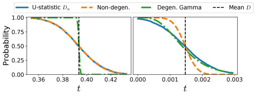
Figure 2: Behaviour of $\mathbb{P}(X>t)$ for $X=D^{\rm MMD}_{n}$ with the RBF kernel versus $X$ being the theoretical limits. Left. $n=1000$ and $d=2$. Right. $n=50$ and $d=1000$.

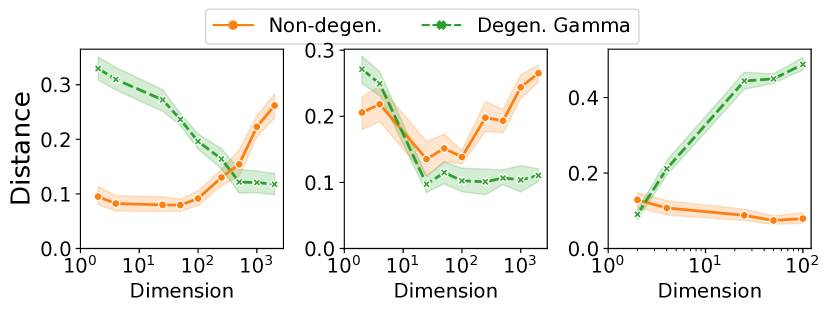
Figure 3: $L_{\infty}$ distance between the c.d.f. of $D^{\rm KSD}_{n}$ with RBF and those of the theoretical limits as $d$ varies. Left. $n=50$ fixed (high dimensions). Middle. $n=\Theta(d^{1/2})$ (high dimensions). Right: $n=\Theta(d^{2})$ (low dimensions).

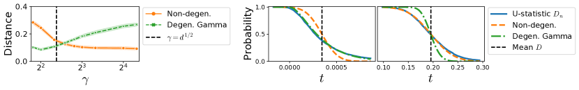
Figure 4: Behaviour of $\mathbb{P}(D^{\rm KSD}_{n}>t)$ with RBF as $\gamma$ varies for $n=50$ and $d=27$. Left. $L_{\infty}$ distance between the c.d.f. of $D^{\rm KSD}_{n}$ and the theoretical limits. Middle. Distribution curves at $\gamma=4$. Right. Distribution curves at $\gamma=16$.

Intriguingly, in both results, different regimes arise based on how $\gamma$ compares with the noise scale $\|\Sigma\|_{2}=d^{1/2}$. In fact, a phase transition as $\gamma$ drops from $\omega(d^{1/2})$ to $o(d^{1/2})$ has been reported in Ramdas et al. (2015) but with no further comments. Our results offer one explanation: Such transitions may happen due to a change in the dependence of $\rho_{d}$ on $\gamma$, $\|\mu\|_{2}$ and $d$. Fig. 4 shows a transition across different limits as $\gamma$ varies, where the transition occurs at around $\gamma\sim d^{1/2}$.

Linear kernel.

Section 3.2 discussed that the limit of $D_{n}$ can be non-Gaussian. This is true for MMD with a linear kernel $\kappa(\mathbf{x},\mathbf{x}^{\prime})=\mathbf{x}^{\top}\mathbf{x}^{\prime}$: It satisfies Lemma 3.13 with $K_{*}=d$ and the limit is a shifted-and-rescaled chi-square. Fig. 1 verifies this for some $\Sigma\neq I_{d}$ by showing an asymmetric distribution curve close to the chi-square limit. We remark that a linear kernel, while not commonly used, is a valid choice here since $D^{\rm MMD}=0$ iff $P=Q$ under our setup.

Simulations.

We set $\mu=(2,0,\ldots,0)^{\top}\in\mathbb{R}^{d}$, $\Sigma=I_{d}$ and $\gamma=\gamma_{\rm med}$ for KSD with RBF and MMD with RBF. The exact setup for MMD with linear kernel is described in Section A.4. The limits for comparison are the non-degenerate Gaussian limit in (3) (“Non-degen.”) and Gamma / shifted-and-rescaled chi-square (“Degen. Gamma” / “Degen. Chi-square”) distributions that match the degenerate limit in Proposition 3.9 by mean and variance. Fig. 1 plots the distribution curves for KSD with RBF and MMD with linear kernel. Fig. 4 plots the same quantity for MMD with RBF. Fig. 4 and Fig. 4 examine the behaviour of KSD with RBF as $d$ or $\gamma$ varies (as a data-independent function of $d$, similar to Ramdas et al. (2015)). Results involving $D_{n}$ are averaged over 30 random seeds, and shaded regions are $95\%$ confidence intervals. Code for reproducing all experiments can be found at https://github.com/XingLLiu/u-stat-high-dim.gitgithub.com/XingLLiu/u-stat-high-dim.git.

KHH is supported by the Gatsby Charitable Foundation. XL is supported by the President’s PhD Scholarships of Imperial College London and the EPSRC StatML CDT programme EP/S023151/1. ABD is supported by Wave 1 of The UKRI Strategic Priorities Fund under the EPSRC Grant EP/T001569/1 and EPSRC Grant EP/W006022/1, particularly the “Ecosystems of Digital Twins” theme within those grants & The Alan Turing Institute. We thank Antonin Schrab, Heishiro Kanagawa and Arthur Gretton for their helpful comments.

The appendix is organised as follows. The first few appendices provide additional content:

Appendix A states additional results for Section 4.3 including moment computations and verification of assumptions.

Appendix B presents auxiliary tools used in subsequent proofs.

The remaining appendices consist of proofs:

Appendix C proves our main theorem. Section C.1 provides a list of intermediate lemmas that extends the proof overview in Section 3.3.

Appendix D proves the remaining results in Section 3.

Appendix E proves the results in Section 4.

Appendices F and G present proofs for the results in Appendices A and B respectively.

Throughout the appendix, we say that $C$ is an absolute constant whenever we mean that it is a number independent of all variables involved, including $u$, $R$, $d$, $n$ and $K$.

Appendix A Additional results for Gaussian mean-shift

In this section, we consider the Gaussian mean-shift setup defined in Section 4.3, where $Q=\mathcal{N}(\mathbf{\mu},\Sigma)$ and $P=\mathcal{N}(0,\Sigma)$ with mean $\mathbf{\mu}\in\mathbb{R}^{d}$ and covariance matrix $\Sigma\in\mathbb{R}^{d\times d}$. We derive analytical expressions of the moments of U-statistics for (i) KSD with RBF, (ii) MMD with RBF and (iii) MMD with linear kernel. We also verify 2 for the three cases, which confirm that our error bounds apply.

Remark on verification of 1.

Recall that 1, which controls the moment ratios $M_{\rm full;\nu}/\sigma_{\rm full}$ and $M_{\rm cond;\nu}/\sigma_{\rm cond}$ for some $\nu\in(2,3]$, is required for our bounds to imply a convergence theorem. As discussed in the main text, this issue is not specific to our theorem and is also relevant to e.g. Berry-Esséen bounds for sample averages of $\{f(\mathbf{X}_{i})\}_{i=1}^{n}$ for $f:\mathbb{R}^{d}\rightarrow\mathbb{R}$ and $d$ large. A detailed verification requires a careful calculation to control the order of $M_{\rm full;\nu},\sigma_{\rm full},M_{\rm cond;\nu}$ and $\sigma_{\rm cond}$. For KSD and MMD with the RBF kernel, a careful control of $\sigma_{\rm full}$ and $\sigma_{\rm cond}$ has already been done in the proof of Proposition 4.5 and Proposition 4.6, which involves examining multiple cases depending on the relative sizes of $\gamma$, $\|\mu\|_{2}$ and $d$ followed by an elaborate calculation. To perform this verification for all cases in full generality, in principle, one may expand on those calculations and follow a similar tedious argument. In the sections below, we perform this verification only for the setup in Fig. 1, i.e. KSD with the RBF kernel in the case $\|\mu\|_{2}=\Theta(1)$ and $\gamma=\Omega(d)$ and MMD with the linear kernel in the general case. For MMD with the RBF kernel, we discuss the relevance of this verification to Gao and Shao (2021), who has done a verification of similar quantities but also in a special case. In Figure 6, we also include simulations verifying 1 under the setups considered in Figure 1-4, where we demonstrate that the moment ratios stay around 1 as the dimension varies from 1 to 2000.

A.1 A decomposition of the RBF kernel

For both MMD and KSD, the key in verifying the assumptions for the RBF kernel is a functional decomposition. The usual Mercer representation of the RBF kernel is available only with respect to a univariate zero-mean Gaussian measure and involves some cumbersome Hermite polynomials. Since we do not actually require orthogonality of the functions in 2, we opt for a simpler functional representation as given below. We also assume WLOG that the bandwidth $\gamma>8$, since we only consider the case $\gamma=\omega(1)$ in our setup.

Lemma A.1.

Assume that $\gamma>8$. Consider two independent $d$-dimensional Gaussian vectors $\mathbf{U}\sim\mathcal{N}(\mu_{1},I_{d})$ and $\mathbf{V}\sim\mathcal{N}(\mu_{2},I_{d})$ for some mean vectors $\mu_{1},\mu_{2}\in\mathbb{R}^{d}$. Then, for any $\nu\in(2,4]$ and $\mu_{1},\mu_{2}\in\mathbb{R}^{d}$, we have that

$$\mathbb{E}\Big{[}\Big{|}\exp\Big{(}-\mfrac{1}{2\gamma}\|\mathbf{U}-\mathbf{V}\|_{2}^{2}\Big{)}-\operatorname{\medmath\prod}_{j=1}^{d}\Big{(}\operatorname{\medmath\sum}_{k=0}^{K}\lambda^{*}_{k}\phi^{*}_{k}(U_{j})\phi^{*}_{k}(V_{j})\Big{)}\Big{|}^{\nu}\Big{]}\;\xrightarrow{K\rightarrow\infty}\;0\;.$$

where $\phi^{*}_{k}(x)\coloneqq x^{k}e^{-x^{2}/(2\gamma)}$ and $\lambda^{*}_{k}\coloneqq\frac{1}{k!\,\gamma^{k}}$ for each $k\in\mathbb{N}\cup\{0\}$.

To see that Lemma A.1 indeed gives the functional decomposition we want in 2, we need to rewrite the product of sums into a sum. To this end, let $g_{d}$ be the $d$-tuple generalisation of the Cantor pairing function from $\mathbb{N}$ to $(\mathbb{N}\cup\{0\})^{d}$ and $[g_{d}(k)]_{l}$ be the $l$-th element of $g_{d}(k)$. Given $\{\lambda^{*}_{l}\}_{l=0}^{\infty}$ and $\{\phi^{*}_{l}\}_{l=0}^{\infty}$ from Lemma A.1, we define, for every $k\in\mathbb{N}$ and $\mathbf{x}=(x_{1},\ldots,x_{d})\in\mathbb{R}^{d}$,

$$\alpha_{k}\;\coloneqq \;\operatorname{\medmath\prod}_{l=1}^{d}\lambda^{*}_{[g_{d}(k)]_{l}} \psi_{k}(\mathbf{x})\;\coloneqq \;\operatorname{\medmath\prod}_{l=1}^{d}\phi^{*}_{[g_{d}(k)]_{l}}(x_{l})\;.$$ and (7)

With this construction, for each $K\in\mathbb{N}$, we can now write

$$\operatorname{\medmath\prod}_{j=1}^{d}\Big{(}\operatorname{\medmath\sum}_{k=0}^{K} \lambda^{*}_{k}\phi^{*}_{k}(U_{j})\phi^{*}_{k}(V_{j})\Big{)}$$

$$\;= \;\operatorname{\medmath\sum}_{k_{1},\ldots,k_{d}=0}^{K}(\lambda^{*}_{k_{1}}\ldots\lambda^{*}_{k_{d}})(\phi^{*}_{k_{1}}(U_{1})\ldots\phi^{*}_{k_{d}}(U_{d}))(\phi^{*}_{k_{1}}(V_{1})\ldots\phi_{k_{d}}(V_{d}))$$

$$\;= \;\operatorname{\medmath\sum}_{k_{1},\ldots,k_{d}=0}^{K}\;\alpha_{g_{d}^{-1}(k_{1},\ldots,k_{d})}\;\psi_{g_{d}^{-1}(k_{1},\ldots,k_{d})}(\mathbf{U})\;\psi_{g_{d}^{-1}(k_{1},\ldots,k_{d})}(\mathbf{V})\;.$$

Since the Cantor pairing function is such that $\min_{l\leq d}[g_{d}(K)]_{l}\rightarrow\infty$ as $K\rightarrow\infty$, Lemma A.1 indeed gives a functional decomposition in terms of $\{\alpha_{k}\}_{k=1}^{\infty}$ and $\{\psi_{k}\}_{k=1}^{\infty}$ as

$$\mathbb{E}\Big{[}\Big{|}\exp\Big{(}-\mfrac{1}{2\gamma}\|\mathbf{U}-\mathbf{V}\|_{2}^{2}\Big{)}-\operatorname{\medmath\sum}_{k=1}^{K}\alpha_{k}\psi_{k}(\mathbf{U})\psi_{k}(\mathbf{V})\Big{|}^{\nu}\Big{]}\;\xrightarrow{K\rightarrow\infty}\;0\;.$$ (8)

We remark that both $\alpha_{k}$ and $\psi_{k}$ are independent of the mean vectors $\mu_{1}$ and $\mu_{2}$, which makes this representation useful for a generic mean-shift setting.

A.2 KSD U-statistic with RBF kernel

Under the Gaussian mean-shift setup with an identity covariance matrix, gradient of the log-density is given by $\nabla\log p(\mathbf{x})=-\mathbf{x}$ for $\mathbf{x}\in\mathbb{R}^{d}$ and the U-statistic for the RBF-kernel KSD is

$$u_{P}^{\rm KSD}(\mathbf{x},\mathbf{x}^{\prime})\;= \;\big{(}\nabla\log p(\mathbf{x})\big{)}^{\top}\big{(}\nabla\log p(\mathbf{x}^{\prime})\big{)}\kappa(\mathbf{x},\mathbf{x}^{\prime})\;+\;\big{(}\nabla\log p(\mathbf{x})\big{)}^{\top}\nabla_{2}\kappa(\mathbf{x},\mathbf{x}^{\prime})$$

$$+\big{(}\nabla\log p(\mathbf{x}^{\prime})\big{)}^{\top}\nabla_{1}\kappa(\mathbf{x},\mathbf{x}^{\prime})\;+\;\text{\rm Tr}(\nabla_{1}\nabla_{2}\kappa(\mathbf{x},\mathbf{x}^{\prime}))$$

$$\;= \;\exp\Big{(}-\mfrac{\|\mathbf{x}-\mathbf{x}^{\prime}\|_{2}^{2}}{2\gamma}\Big{)}\Big{(}\mathbf{x}^{\top}\mathbf{x}^{\prime}+\mfrac{1}{\gamma}\mathbf{x}^{\top}(\mathbf{x}^{\prime}-\mathbf{x})+\mfrac{1}{\gamma}(\mathbf{x}^{\prime})^{\top}(\mathbf{x}-\mathbf{x}^{\prime})+\Big{(}\mfrac{d}{\gamma}-\mfrac{\|\mathbf{x}-\mathbf{x}^{\prime}\|_{2}^{2}}{\gamma^{2}}\Big{)}\Big{)}$$

$$\;= \;\exp\Big{(}-\mfrac{\|\mathbf{x}-\mathbf{x}^{\prime}\|_{2}^{2}}{2\gamma}\Big{)}\Big{(}\mathbf{x}^{\top}\mathbf{x}^{\prime}-\mfrac{\gamma+1}{\gamma^{2}}\|\mathbf{x}-\mathbf{x}^{\prime}\|_{2}^{2}+\mfrac{d}{\gamma}\Big{)}\;.$$ (9)

We first verify that 2 holds by adapting $\{\alpha_{k}\}_{k=1}^{\infty}$ and $\{\psi_{k}\}_{k=1}^{\infty}$ from Section A.1.

Lemma A.2.

Assume that $\gamma>24$. For $k^{\prime}\in\mathbb{N}$, consider

$$\lambda_{(k^{\prime}-1)(d+3)+1}\;=\;-\mfrac{\gamma+1}{\gamma^{2}}\alpha_{k^{\prime}}\;, \phi_{(k^{\prime}-1)(d+3)+1}(\mathbf{x})\;=\;\psi_{k^{\prime}}(\mathbf{x})(\|\mathbf{x}\|_{2}^{2}+1)\;,$$

$$\lambda_{(k^{\prime}-1)(d+3)+2}\;=\;\mfrac{\gamma+1}{\gamma^{2}}\alpha_{k^{\prime}}\;, \phi_{(k^{\prime}-1)(d+3)+2}(\mathbf{x})\;=\;\psi_{k^{\prime}}(\mathbf{x})\|\mathbf{x}\|_{2}^{2}\;,$$

$$\lambda_{(k^{\prime}-1)(d+3)+3}\;=\;\Big{(}\mfrac{d}{\gamma}+\mfrac{\gamma+1}{\gamma^{2}}\Big{)}\alpha_{k^{\prime}}\;, \phi_{(k^{\prime}-1)(d+3)+3}(\mathbf{x})\;=\;\psi_{k^{\prime}}(\mathbf{x})\;,$$

and for $l=1,\ldots,d$, define

$$\lambda_{(k^{\prime}-1)(d+3)+3+l}\;=\;\mfrac{\gamma^{2}+2\gamma+2}{\gamma^{2}}\alpha_{k^{\prime}}\;, \phi_{(k^{\prime}-1)(d+3)+3+l}(\mathbf{x})\;=\;\psi_{k^{\prime}}(\mathbf{x})x_{l}\;.$$

Then 2 holds with any $\nu\in(2,3]$ for $u=u_{P}^{\rm KSD}$, $\{\lambda_{k}\}_{k=1}^{\infty}$ and $\{\phi_{k}\}_{k=1}^{\infty}$ defined above.

The following result (proved in Appendix F.2) provides analytical forms or upper bounds for the moments of KSD U-statistic.

Lemma A.3 (KSD moments).

Let $\kappa$ be a RBF kernel with bandwidth $\gamma=\omega(1)$, and let $\mathbf{X},\mathbf{X}^{\prime}$ be independent draws from $Q$. Under the mean-shift setup with an identity covariance matrix, it follows that

1. For every $\mathbf{x}\in\mathbb{R}^{d}$,

   $$g^{\rm KSD}(\mathbf{x})\;\coloneqq \;\mathbb{E}[u_{P}^{\rm KSD}(\mathbf{x},\mathbf{X}^{\prime})]$$

   $$\;= \;\left(\mfrac{\gamma}{\gamma+1}\right)^{d/2}\exp\left(-\mfrac{1}{2(\gamma+1)}\|\mathbf{x}-\mathbf{\mu}\|_{2}^{2}\right)\left(\mfrac{2+\gamma}{1+\gamma}\mathbf{\mu}^{\top}\mathbf{x}-\mfrac{1}{1+\gamma}\|\mathbf{\mu}\|_{2}^{2}\right)\;;$$

2. The mean is given by $D^{\rm KSD}(Q,P)=\left(\mfrac{\gamma}{\gamma+2}\right)^{d/2}\|\mu\|_{2}^{2}$ ;

3. The variance of the conditional expectation $g^{\rm KSD}(\mathbf{X})$ is given by

   $$\sigma_{\rm cond}^{2}\;= \;\left(\mfrac{\gamma^{2}}{(1+\gamma)(3+\gamma)}\right)^{d/2}\bigg{(}\mfrac{(2+\gamma)^{2}}{(1+\gamma)(3+\gamma)}\|\mathbf{\mu}\|_{2}^{2}+\left(1-\left(\mfrac{(1+\gamma)(3+\gamma)}{(2+\gamma)^{2}}\right)^{d/2}\right)\|\mathbf{\mu}\|_{2}^{4}\bigg{)}\;;$$

4. The variance of $u_{P}^{\rm KSD}(\mathbf{X},\mathbf{X}^{\prime})$ is given by

   $$\sigma_{\rm full}^{2}\;= \;\left(\mfrac{\gamma}{4+\gamma}\right)^{d/2}\bigg{(}d+\mfrac{d^{2}}{\gamma^{2}}+\mfrac{2d\|\mathbf{\mu}\|_{2}^{2}}{\gamma}+2\|\mathbf{\mu}\|_{2}^{2}+\left(1-\left(\mfrac{\gamma(4+\gamma)}{(2+\gamma)^{2}}\right)^{d/2}\right)\|\mathbf{\mu}\|_{2}^{4}$$

   $$\qquad\qquad\qquad\;+o\left(d+\mfrac{d^{2}}{\gamma^{2}}+\mfrac{d\|\mathbf{\mu}\|_{2}^{2}}{\gamma}+\|\mathbf{\mu}\|_{2}^{2}\right)\bigg{)}\;;$$

5. For any $\nu>2$, there exist positive constants $C_{1},C_{2}$ depending only on $\nu$ such that the $\nu$-th absolute moment of the conditional expectation satisfies

   $$\mathbb{E}[|g^{\rm KSD}(\mathbf{X})|^{\nu}]\;\leq\;\left(\mfrac{\gamma}{1+\gamma}\right)^{\nu d/2}\left(\mfrac{1+\gamma}{1+\nu+\gamma}\right)^{d/2}(C_{1}\|\mu\|_{2}^{\nu}+C_{2}\|\mu\|_{2}^{2\nu})\;.$$

6. For any $\nu>2$, there exist positive constants $C_{3},C_{4},C_{5},C_{6}$ depending only on $\nu$ such that the $\nu$-th absolute moment of $u_{P}^{\rm KSD}(\mathbf{X},\mathbf{X}^{\prime})$ satisfies

   $$\mathbb{E}[|u_{P}^{\rm KSD}(\mathbf{X},\mathbf{X}^{\prime})|^{\nu}]\; \leq\;\left(\mfrac{\gamma}{2\nu+\gamma}\right)^{d/2}\Big{(}C_{3}d^{\nu/2}+C_{4}\Big{(}\mfrac{d}{\gamma}\Big{)}^{\nu}+C_{5}\|\mathbf{\mu}\|_{2}^{\nu}+C_{6}\|\mathbf{\mu}\|_{2}^{2\nu}$$

   $$\qquad\qquad\qquad\quad\;\;+o\Big{(}d^{\nu/2}+\mfrac{d^{\nu}}{\gamma^{\nu}}+\mfrac{\|\mathbf{\mu}\|_{2}^{2\nu}}{\gamma^{\nu}}\Big{)}\Big{)}\;.$$

In particular, when $\|\mu\|_{2}=\Theta(1)$ and $\gamma=\Omega(d)$, 1 holds with any $\nu>2$ for $u_{P}^{\rm KSD}$ under $Q$.

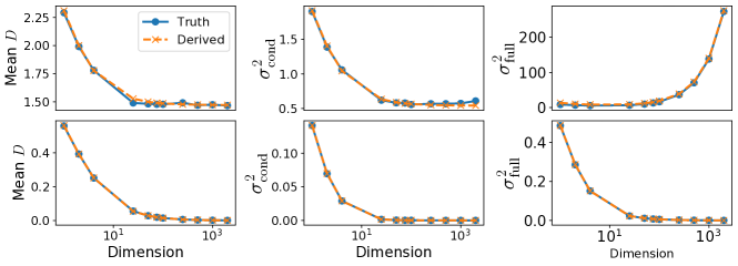
Figure 5: Verifying the analytical expressions for the first two moments of KSD and MMD. Top. KSD moments derived in Lemma A.3. Bottom. MMD moments derived in Lemma A.5. The ground truth is estimated using $n=4000$ samples for KSD and $n=10000$ samples for MMD, respectively, and the reported results are averaged over 5 random seeds.

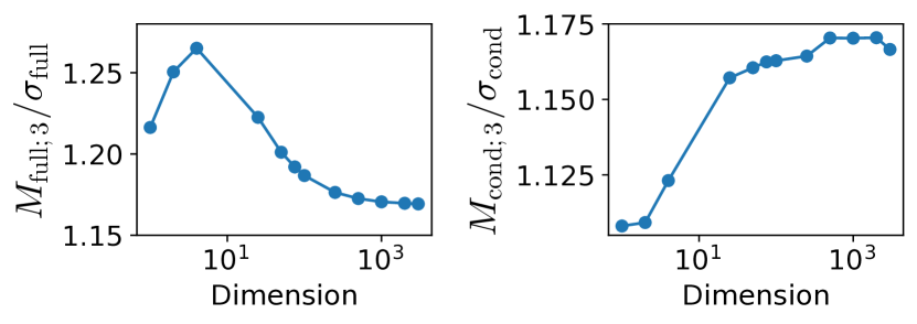
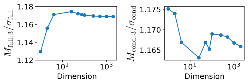
Figure 6: Verifying 1 for $\nu=3$ for KSD and MMD with RBF kernels. All moment ratios appear to be bounded by a dimension-independent constant. Left and middle-left. KSD moment ratios. Middle-right and right. MMD moment ratios. The reported results are averaged over 5 random seeds.

A.3 MMD U-statistic with RBF kernel

Under the Gaussian mean-shift setup with an identity covariance matrix, the MMD U-statistic with a RBF kernel has the form

$$u^{\rm MMD}(\mathbf{z},\mathbf{z}^{\prime})\;=\;\kappa(\mathbf{x},\mathbf{x}^{\prime})+\kappa(\mathbf{y},\mathbf{y}^{\prime})-\kappa(\mathbf{x},\mathbf{y}^{\prime})-\kappa(\mathbf{x}^{\prime},\mathbf{y})$$

$$=\;\exp\left(-\mfrac{\|\mathbf{x}-\mathbf{x}^{\prime}\|_{2}^{2}}{2\gamma}\right)+\exp\left(-\mfrac{\|\mathbf{y}-\mathbf{y}^{\prime}\|_{2}^{2}}{2\gamma}\right)-\exp\left(-\mfrac{\|\mathbf{x}-\mathbf{y}^{\prime}\|_{2}^{2}}{2\gamma}\right)-\exp\left(-\mfrac{\|\mathbf{x}^{\prime}-\mathbf{y}\|_{2}^{2}}{2\gamma}\right)\;,$$ (10)

for $\mathbf{z}\coloneqq(\mathbf{x},\mathbf{y}),\mathbf{z}^{\prime}\coloneqq(\mathbf{x}^{\prime},\mathbf{y}^{\prime})\in\mathbb{R}^{2d}$. We first verify that 2 holds again by adapting $\{\alpha_{k}\}_{k=1}^{\infty}$ and $\{\psi_{k}\}_{k=1}^{\infty}$ from Section A.1.

Lemma A.4.

Assume that $\gamma>8$. Then 2 holds with any value $\nu\in(2,3]$ and the function $u((\mathbf{x},\mathbf{y}),(\mathbf{x}^{\prime},\mathbf{y}^{\prime}))=u^{\rm MMD}((\mathbf{x},\mathbf{y}),(\mathbf{x}^{\prime},\mathbf{y}^{\prime}))$ for $\mathbf{x},\mathbf{y},\mathbf{x}^{\prime},\mathbf{y}^{\prime}\in\mathbb{R}^{d}$, with the sequences of values and functions given for each $k\in\mathbb{N}$ as $\gamma_{k}=\alpha_{k}$ and $\phi_{k}(\mathbf{x},\mathbf{y})=\psi_{k}(\mathbf{x})-\psi_{k}(\mathbf{y})$.

We next compute the moments. The analytical form of the population MMD (i.e. the expectation) has been derived in previous works under both the Gaussian mean-shift setup with a general covariance matrix $\Sigma$ (Wynne and Duncan (2022, Proposition 2, Corollary 19); (Ramdas et al., 2015, Proposition 1)) and an expression up to the learning term was also derived under a more general mean-shift setup (Reddi et al., 2015, Lemma 1). We only consider the Gaussian mean-shift case with $\Sigma=I_{d}$ but provide expressions for the second moments and a generic moment bound, while making minimal assumptions on the kernel bandwidth compared to Reddi et al. (2015).

Lemma A.5 (RBF-MMD moments).

Let $\kappa$ be a RBF kernel and let $\mathbf{X},\mathbf{X}^{\prime}\sim Q$ and $\mathbf{Y},\mathbf{Y}^{\prime}\sim P$ be mutually independent draws. Under the mean-shift setup with an identity covariance matrix, it follows that

1. For every $\mathbf{z}=(\mathbf{x},\mathbf{y})\in\mathbb{R}^{2d}$,

   $$g^{\rm mmd} (\mathbf{z})\;\coloneqq\;\mathbb{E}[u^{\rm MMD}(\mathbf{z},\mathbf{Z}^{\prime})]$$

   $$=\left(\mfrac{\gamma}{1+\gamma}\right)^{d/2}\Big{(}e^{-\frac{1}{2(1+\gamma)}\|\mathbf{x}-\mathbf{\mu}\|_{2}^{2}}+e^{-\frac{1}{2(1+\gamma)}\|\mathbf{y}\|_{2}^{2}}-e^{-\frac{1}{2(1+\gamma)}\|\mathbf{x}\|_{2}^{2}}-e^{-\frac{1}{2(1+\gamma)}\|\mathbf{y}-\mathbf{\mu}\|_{2}^{2}}\Big{)}\;;$$

2. The mean is given by $D^{\rm MMD}(Q,P)\;=\;2\left(\mfrac{\gamma}{2+\gamma}\right)^{d/2}\Big{(}1-\exp\left(-\mfrac{1}{2(2+\gamma)}\|\mu\|_{2}^{2}\right)\Big{)}\;;$

3. The variance of the conditional expectation is given by

   $$\sigma_{\rm cond}^{2}\; =\;2\left(\mfrac{\gamma}{1+\gamma}\right)^{d/2}\left(\mfrac{\gamma}{3+\gamma}\right)^{d/2}$$

   $$\;\quad\times\bigg{(}1+\exp\left(-\mfrac{1}{3+\gamma}\|\mu\|_{2}^{2}\right)+2\left(\mfrac{3+\gamma}{2+\gamma}\right)^{d/2}\left(\mfrac{1+\gamma}{2+\gamma}\right)^{d/2}\exp\left(-\mfrac{1}{2(2+\gamma)}\|\mu\|_{2}^{2}\right)$$

   $$\qquad\quad-2\exp\left(-\mfrac{7+5\gamma}{4(1+\gamma)(3+\gamma)}\|\mu\|_{2}^{2}\right)-\left(\mfrac{3+\gamma}{2+\gamma}\right)^{d/2}\left(\mfrac{1+\gamma}{2+\gamma}\right)^{d/2}$$

   $$\qquad\quad-\left(\mfrac{3+\gamma}{2+\gamma}\right)^{d/2}\left(\mfrac{1+\gamma}{2+\gamma}\right)^{d/2}\exp\left(-\mfrac{1}{2+\gamma}\|\mu\|_{2}^{2}\right)\bigg{)}\;;$$

4. The variance is given by

   $$\sigma_{\rm full}^{2}\; =\;2\left(\mfrac{\gamma}{4+\gamma}\right)^{d/2}\bigg{(}1+\exp\left(-\mfrac{1}{4+\gamma}\|\mu\|_{2}^{2}\right)\bigg{)}-2\left(\mfrac{\gamma}{2+\gamma}\right)^{d}$$

   $$\;\quad-8\left(\mfrac{\gamma}{3+\gamma}\right)^{d/2}\left(\mfrac{\gamma}{1+\gamma}\right)^{d/2}\exp\left(-\mfrac{2+\gamma}{2(1+\gamma)(3+\gamma)}\|\mu\|_{2}^{2}\right)$$

   $$\;\quad-2\left(\mfrac{\gamma}{2+\gamma}\right)^{d}\exp\left(-\mfrac{1}{2+\gamma}\|\mu\|_{2}^{2}\right)+8\left(\mfrac{\gamma}{2+\gamma}\right)^{d}\exp\left(-\mfrac{1}{2(2+\gamma)}\|\mathbf{\mu}\|_{2}^{2}\right)\;.$$

While we do not verify 1 here, we remark that Gao and Shao (2021) also encounter similar moment ratios when deriving finite-sample bounds for MMD with a studentised version of U-statistic (see e.g. their Theorem 13). They show that those ratios are controlled under an elaborate list of assumptions; in particular, those assumptions hold for the RBF kernel under a condition that amounts to choosing $\gamma=\Theta(d)$ in our Gaussian mean-shift setup. For our case, as discussed, a rigorous verification of 1 can be done by following the proofs of Propositions 4.5 and 4.6 to control $M_{\rm cond;\nu}$ and $M_{\rm full;\nu}$ for any $\nu>2$. Fig. 6 also verifies 1 by simulation.

A.4 MMD U-statistic with linear kernel

In this section, we consider the mean-shift setup with a general covariance matrix $\Sigma\in\mathbb{R}^{d\times d}$, i.e., $Q=\mathcal{N}(\mathbf{\mu},\Sigma)$ and $P=\mathcal{N}(0,\Sigma)$. The MMD with a linear kernel $\kappa(\mathbf{x},\mathbf{x}^{\prime})=\mathbf{x}^{\top}\mathbf{x}^{\prime}$ has the form

$$u^{\rm MMD}(\mathbf{z},\mathbf{z}^{\prime})\;= \;\mathbf{x}^{\top}\mathbf{x}^{\prime}+\mathbf{y}^{\top}\mathbf{y}^{\prime}-\mathbf{x}^{\top}\mathbf{y}^{\prime}-\mathbf{y}^{\top}\mathbf{x}^{\prime}\;,$$

where $\mathbf{z}\coloneqq(\mathbf{x},\mathbf{y}),\mathbf{z}^{\prime}\coloneqq(\mathbf{x}^{\prime},\mathbf{y}^{\prime})\in\mathbb{R}^{2d}$. In this case, 2 holds directly because we can represent $u^{\rm MMD}$ as

$$u^{\rm MMD}(\mathbf{z},\mathbf{z}^{\prime})\;=\;(\mathbf{x}-\mathbf{y})^{\top}(\mathbf{x}^{\prime}-\mathbf{y}^{\prime})\;=\;\operatorname{\medmath\sum}_{l=1}^{d}(x_{l}-y_{l})(x^{\prime}_{l}-y^{\prime}_{l})\;=\;\operatorname{\medmath\sum}_{l=1}^{d}\gamma_{l}\psi_{l}(\mathbf{z})\psi_{l}(\mathbf{z}^{\prime})\;,$$ (11)

where $\gamma_{l}=1$, $\psi_{l}(\mathbf{z})=x_{l}-y_{l}$ and $\psi_{l}(\mathbf{z}^{\prime})=x^{\prime}_{l}-y^{\prime}_{l}$.

We next compute the moment terms and verify that 1 holds. The next result, proved in Section F.4, gives the analytical expressions of the first two moments of the linear-kernel MMD.

Lemma A.6 (Linear-MMD moments).

Let $\kappa$ be a linear kernel, and let $\mathbf{X},\mathbf{X}^{\prime}\sim Q$ and $\mathbf{Y},\mathbf{Y}^{\prime}\sim P$ be mutually independent draws. Write $\mathbf{Z}=(\mathbf{X},\mathbf{Y})$ and $\mathbf{Z}^{\prime}=(\mathbf{X}^{\prime},\mathbf{Y}^{\prime})$. Under the mean-shift setup, it follows that

1. For every $\mathbf{z}=(\mathbf{x},\mathbf{y})\in\mathbb{R}^{2d}$, we have $g^{\rm mmd}(\mathbf{z})\coloneqq\mathbb{E}[u^{\rm MMD}(\mathbf{z},\mathbf{Z}^{\prime})]=\mathbf{\mu}^{\top}\mathbf{y}-\mathbf{\mu}^{\top}\mathbf{x}$ ;

2. The mean is given by $D^{\rm MMD}(Q,P)=\|\mathbf{\mu}\|_{2}^{2}$ ;

3. The variance of the conditional expectation $g^{\rm mmd}(\mathbf{Z})$ is given by $\sigma_{\rm cond}^{2}=2\mathbf{\mu}^{\top}\Sigma\mathbf{\mu}$ ;

4. The variance of $u^{\rm MMD}(\mathbf{Z},\mathbf{Z}^{\prime})$ is given by $\sigma_{\rm full}^{2}=4\text{\rm Tr}(\Sigma^{2})+4\mathbf{\mu}^{\top}\Sigma\mathbf{\mu}$ ;

5. The third central moment of $g^{\rm mmd}(\mathbf{Z})$ satisfies $M_{\rm cond;3}^{3}\leq C(\mu^{\top}\Sigma\mu)^{3/2}$ for some absolute constant $C$ ;

6. The third central moment of $u^{\rm MMD}(\mathbf{Z},\mathbf{Z}^{\prime})$ satisfies $M_{\rm full;3}^{3}\leq C\big{(}\text{\rm Tr}(\Sigma^{2})+\mu^{\top}\Sigma\mu\big{)}^{3/2}$ for some absolute constant $C$ .

In particular, 1 holds with $\nu=3$ for $u^{\rm MMD}$ defined in (11) under $Q$.

In the last example in Section 4.3, we chose $\mu=(0,10,\ldots,0)\in\mathbb{R}^{d}$ and a diagonal $\Sigma$ with $\Sigma_{11}=0.5(d+1)$, $\Sigma_{ii}=0.5$ for $i>1$ and $\Sigma_{ij}=0$ otherwise. Note that by the invariance of Gaussian distributions under orthogonal transformation, this is equivalent to choosing $\Sigma$ as $0.5\mathbf{I}_{d}+0.5\mathbf{J}_{d}$, where $\mathbf{I}_{d}\in\mathbb{R}^{d\times d}$ is the identity matrix, $\mathbf{J}_{d}\in\mathbb{R}^{d\times d}$ is the all-one matrix and $\mu$ is transformed by an appropriate orthogonal matrix of eigenvectors. Notably, this choice ensures the limit of $u^{\rm MMD}$ remains non-Gaussian. Indeed, when $Q$ and $P$ are Gaussian, the statistic $D^{\rm MMD}_{n}$ can be written as a sum of shifted-and-rescaled chi-squares, where the scaling factors are $0.5(d+1),0.5,\ldots,0.5$, the eigenvalues of $\Sigma$. As $d$ grows, the eigenvalue $0.5(d+1)$ dominates, and the limiting distribution is then dominated by the first summand, thereby yielding a chi-square limit up to shifting and rescaling. This is numerically demonstrated in the right figure of Fig. 1. As a remark, we do not expect this exact setting to occur in practice; it should instead be treated as a toy setup to demonstrate the possibility of non-Gaussianity and convey an intuition of when this may occur.

Appendix B Auxiliary tools

B.1 Generic moment bounds

We first present two-sided bounds on the moments of a martingale, which are useful in bounding $\nu$-th moment terms of different statistics. The original result is due to Burkholder (1966), and the constant $C_{\nu}$ is provided by von Bahr and Esseen (1965) and Dharmadhikari et al. (1968).

Lemma B.1.

Fix $\nu>1$. For a martingale difference sequence $Y_{1},\ldots,Y_{n}$ taking values in $\mathbb{R}$,

$$c_{\nu}\,n^{\min\{0,\nu/2-1\}}\operatorname{\medmath\sum}_{i=1}^{n}\mathbb{E}[|Y_{i}|^{\nu}]\;\leq\;\mathbb{E}\big{[}\big{|}\operatorname{\medmath\sum}_{i=1}^{n}Y_{i}\big{|}^{\nu}\big{]}\;\leq\;C_{\nu}\,n^{\max\{0,\nu/2-1\}}\operatorname{\medmath\sum}_{i=1}^{n}\mathbb{E}[|Y_{i}|^{\nu}]\;,$$

for $C_{\nu}:=\max\big{\{}2,(8(\nu-1)\max\{1,2^{\nu-3}\})^{\nu}\big{\}}$ and some absolute constant $c_{\nu}>0$ that depends only on $\nu$.

The next moment computation for a quadratic form of Gaussians is used throughout the proof:

Lemma B.2 (Lemma 2.3, Magnus (1978)).

Given a standard Gaussian vector $\eta$ in $\mathbb{R}^{m}$ and a symmetric $m\times m$ matrix $A$, we have that $\mathbb{E}[\eta^{\top}A\eta]=\text{\rm Tr}(A)$ and

$$\mathbb{E}[(\eta^{\top}A\eta)^{2}]\;=\;\text{\rm Tr}(A)^{2}+2\text{\rm Tr}(A^{2})\;, \mathbb{E}[(\eta^{\top}A\eta)^{3}]\;=\;\text{\rm Tr}(A)^{3}+6\text{\rm Tr}(A)\text{\rm Tr}(A^{2})+8\text{\rm Tr}(A^{3})\;.$$

The next two results are used for the moment computation involving an RBF kernel.

Lemma B.3.

Fix $\mathbf{m}_{i}\in\mathbb{R}^{d}$ and $a_{i}>0$ for $i=1,2$. Let $\mathbf{X}\sim\mathcal{N}(\mathbf{m}_{1},a_{1}^{2}I_{d})$, and let $f:\mathbb{R}^{d}\to\mathbb{R}$ be a deterministic function such that $\mathbb{E}[|f(\mathbf{X})|]<\infty$. It follows that

$$\mathbb{E}\Big{[}f(\mathbf{X})\exp\Big{(}-\mfrac{\|\mathbf{X}-\mathbf{m}_{2}\|_{2}^{2}}{2a_{2}^{2}}\Big{)}\Big{]}\; =\;\Big{(}\mfrac{a_{2}^{2}}{a_{1}^{2}+a_{2}^{2}}\Big{)}^{d/2}\exp\Big{(}-\mfrac{\|\mathbf{m}_{1}-\mathbf{m}_{2}\|_{2}^{2}}{2(a_{1}^{2}+a_{2}^{2})}\Big{)}\mathbb{E}[f(\mathbf{W})]\;,$$

where $\mathbf{W}\sim\mathcal{N}(\mathbf{m},a^{2}I_{d})$ with $\,\mathbf{m}\;\coloneqq\;\frac{a_{1}^{2}a_{2}^{2}}{a_{1}^{2}+a_{2}^{2}}\big{(}\frac{1}{a_{1}^{2}}\mathbf{m}_{1}+\frac{1}{a_{2}^{2}}\mathbf{m}_{2}\big{)}$ and $a^{2}\coloneqq\frac{a_{1}^{2}a_{2}^{2}}{a_{1}^{2}+a_{2}^{2}}$ .

Lemma B.4.

Fix $\mathbf{m}_{1},\mathbf{m}_{2}\in\mathbb{R}^{d}$ and $a_{i}>0$ for $i=1,2,3$. Let $\mathbf{X}\sim\mathcal{N}(\mathbf{m}_{1},a_{1}^{2}I_{d})$ and $\mathbf{X}^{\prime}\sim\mathcal{N}(\mathbf{m}_{2},a_{2}^{2}I_{d})$, and let $f:\mathbb{R}^{d}\times\mathbb{R}^{d}\to\mathbb{R}$ be a deterministic function with $\mathbb{E}[|f(\mathbf{X},\mathbf{X}^{\prime})|]<\infty$. Then

$$\mathbb{E}\Big{[}f(\mathbf{X},\mathbf{X}^{\prime}) \exp\left(-\mfrac{\|\mathbf{X}-\mathbf{X}^{\prime}\|_{2}^{2}}{2a_{3}^{2}}\right)\Big{]}$$

$$\;= \;\Big{(}\mfrac{a_{3}^{2}}{a_{1}^{2}+a_{2}^{2}+a_{3}^{2}}\Big{)}^{d/2}\exp\Big{(}-\mfrac{\|\mathbf{m}_{1}-\mathbf{m}_{2}\|_{2}^{2}}{2(a_{1}^{2}+a_{2}^{2}+a_{3}^{2})}\Big{)}\mathbb{E}\Big{[}f\Big{(}\mathbf{W},\mathbf{W}^{\prime}+\mfrac{a_{2}^{2}}{a_{2}^{2}+a_{3}^{2}}\mathbf{W}\Big{)}\Big{]}\;,$$

where $\mathbf{W}\sim\mathcal{N}\left(\mathbf{m},a^{2}I_{d}\right)$ and $\mathbf{W}^{\prime}\sim\mathcal{N}\left(\mathbf{m}^{\prime},(a^{\prime})^{2}I_{d}\right)$ are independent with

$$\mathbf{m}\;\coloneqq \;\mfrac{a_{1}^{2}(a_{2}^{2}+a_{3}^{2})}{a_{1}^{2}+a_{2}^{2}+a_{3}^{2}}\left(\mfrac{1}{a_{1}^{2}}\mathbf{m}_{1}+\mfrac{1}{a_{2}^{2}+a_{3}^{2}}\mathbf{m}_{2}\right)\;, \quad a^{2}\;\coloneqq\;\mfrac{a_{1}^{2}(a_{2}^{2}+a_{3}^{2})}{a_{1}^{2}+a_{2}^{2}+a_{3}^{2}}\;,$$

$$\mathbf{m}^{\prime}\;\coloneqq \;\mfrac{a_{3}^{2}}{a_{2}^{2}+a_{3}^{2}}\mathbf{m}_{2}\;, (a^{\prime})^{2}\;\coloneqq\;\mfrac{a_{2}^{2}a_{3}^{2}}{a_{2}^{2}+a_{3}^{2}}\;.$$

B.2 Moment bounds for U-statistics

We first present a result that bounds the moments of a U-statistic $D_{n}$ defined as in (LABEL:eqn:general:u:defn).

Lemma B.5.

Fix $n\geq 2$ and $\nu\geq 2$. Then, there exist absolute constants $c_{\nu},C_{\nu}>0$ depending only on $\nu$ such that

$$\mathbb{E}[|D_{n}-\mathbb{E}D_{n}|^{\nu}]\; \leq\;C_{\nu}\,n^{\nu/2}(n-1)^{-\nu}M_{\rm cond;\nu}^{\nu}+C_{\nu}\,(n-1)^{-\nu}M_{\rm full;\nu}^{\nu}\;,$$

$$\mathbb{E}[|D_{n}-\mathbb{E}D_{n}|^{\nu}]\; \geq\;c_{\nu}n(n-1)^{-\nu}M_{\rm cond;\nu}^{\nu}+c_{\nu}n^{-(\nu-1)}(n-1)^{-(\nu-1)}M_{\rm full;\nu}^{\nu}\;.$$

In other words,

$$\mathbb{E}[|D_{n}-\mathbb{E}D_{n}|^{\nu}]\; =\;O(n^{-\nu/2}M_{\rm cond;\nu}^{\nu}+n^{-\nu}M_{\rm full;\nu}^{\nu})\;,$$

$$\mathbb{E}[|D_{n}-\mathbb{E}D_{n}|^{\nu}]\; =\;\Omega(n^{-(\nu-1)}M_{\rm cond;\nu}^{\nu}+n^{-2(\nu-1)}M_{\rm full;\nu}^{\nu})\;.$$

The next two results summarise how the moments of variables under the functional decomposition in 2 interact with the moments of the original statistic $u$ under $R$:

Lemma B.6.

Let $\{\phi_{k}\}_{k=1}^{\infty}$, $\{\lambda_{k}\}_{k=1}^{\infty}$ and $\varepsilon_{K;\nu}$ be defined as in 2. For $\mathbf{X}_{1},\mathbf{X}_{2}\overset{i.i.d.}{\sim}R$, write $\mu_{k}\coloneqq\mathbb{E}[\phi_{k}(\mathbf{X}_{1})]$ and let the moment terms $D,M_{\rm cond;\nu},M_{\rm full;\nu}$ be defined as in Section 2.1. Then we have the following:

1. $\big{|}\sum_{k=1}^{K}\lambda_{k}\mu_{k}^{2}-D\big{|}\leq\varepsilon_{K;1}$;

2. for any $\nu\in[1,3]$, we have that

   $$\mfrac{1}{4}(M_{\rm cond;\nu})^{\nu}-\varepsilon_{K;\nu}^{\nu}\;\leq\;\mathbb{E}\Big{[}\Big{|}\operatorname{\medmath\sum}_{k=1}^{K}\lambda_{k}(\phi_{k}(\mathbf{X}_{1})-\mu_{k})\mu_{k}\Big{|}^{\nu}\Big{]}\;\leq\;4((M_{\rm cond;\nu})^{\nu}+\varepsilon_{K;\nu}^{\nu})\;;$$

3. there exist some absolute constants $c,C>0$ such that

$$\mathbb{E}\Big{[}\Big{|}\operatorname{\medmath\sum}_{k=1}^{K}\lambda_{k}(\phi_{k}(\mathbf{X}_{1})-\mu_{k})(\phi_{k}(\mathbf{X}_{2})-\mu_{k})\Big{|}^{\nu}\Big{]}\leq \;4C(M_{\rm full;\nu})^{\nu}-\mfrac{1}{2}(M_{\rm cond;\nu})^{\nu}+(4C+2)\varepsilon_{K;\nu}^{\nu}\;,$$

$$\mathbb{E}\Big{[}\Big{|}\operatorname{\medmath\sum}_{k=1}^{K}\lambda_{k}(\phi_{k}(\mathbf{X}_{1})-\mu_{k})(\phi_{k}(\mathbf{X}_{2})-\mu_{k})\Big{|}^{\nu}\Big{]}\geq \;\mfrac{c}{4}(M_{\rm full;\nu})^{\nu}-8(M_{\rm cond;\nu})^{\nu}-(c+8)\varepsilon_{K;\nu}^{\nu}\;.$$

The next result assumes the notations of Lemma B.6, and additionally denotes

$$\Lambda^{K}\;\coloneqq\;\text{\rm diag}\{\lambda_{1},\ldots,\lambda_{K}\}\;\in\mathbb{R}^{K\times K}\;, \phi^{K}(x)\;\coloneqq\;(\phi_{1}(x),\ldots,\phi_{K}(x))^{\top}\;\in\mathbb{R}^{K}\;.$$

Lemma B.7.

For $\mu^{K}\coloneqq\mathbb{E}[\phi^{K}(\mathbf{X}_{1})]$ and $\Sigma^{K}\coloneqq\text{\rm Cov}[\phi^{K}(\mathbf{X}_{1})]$, we have

$$\sigma_{\rm cond}^{2}-4\sigma_{\rm cond}\varepsilon_{K;2}-4\varepsilon_{K;2}^{2}\;\leq\; (\mu^{K})^{\top}\Lambda^{K}\Sigma^{K}\Lambda^{K}(\mu^{K})\;\leq\;(\sigma_{\rm cond}+2\varepsilon_{K;2})^{2}\;.$$

$$(\sigma_{\rm full}-\varepsilon_{K;2})^{2}\;\leq\; \text{\rm Tr}((\Lambda^{K}\Sigma^{K})^{2})\;\leq\;(\sigma_{\rm full}+\varepsilon_{K;2})^{2}\;.$$

In particular, for $\nu\in[1,3]$ and two i.i.d. zero-mean Gaussian vector $\mathbf{Z}_{1}$ and $\mathbf{Z}_{2}$ in $\mathbb{R}^{K}$ with variance $\Sigma^{K}$, there exists some absolute constant $C>0$ such that

$$\mathbb{E}[|(\mu^{K})^{\top}\Lambda^{K}\mathbf{Z}_{1}|^{\nu}]\;\leq\;7\big{(}\sigma_{\rm cond}^{\nu}+8\varepsilon_{K;2}^{\nu}\big{)}\;,\qquad\mathbb{E}[|\mathbf{Z}_{1}^{\top}\Lambda^{K}\mathbf{Z}_{2}|^{\nu}]\;\leq\;6\big{(}\sigma_{\rm full}^{\nu}+\varepsilon_{K;2}^{\nu}\big{)}\;,$$

$$\mathbb{E}\big{[}\big{|}(\phi^{K}(\mathbf{X}_{1})-\mu^{K})^{\top}\Lambda^{K}\mathbf{Z}_{1}\big{|}^{\nu}\big{]}\;\leq\;8C(M_{\rm full;\nu})^{\nu}-(M_{\rm cond;\nu})^{\nu}+(8C+4)\varepsilon_{K;\nu}^{\nu}\;.$$

The next lemma gives an equivalent expression for $W_{n}^{K}$ defined in (5) and also controls the moments of $W_{n}^{K}$.

Lemma B.8.

Let $\{\eta^{K}_{i}\}_{i=1}^{n}$ be a sequence of i.i.d. standard Gaussian vectors in $\mathbb{R}^{K}$. Then

1. the distribution of $W_{n}^{K}$ satisfies

   $$W_{n}^{K}\;\overset{d}{=}\;\mfrac{1}{n^{3/2}(n-1)^{1/2}}\Big{(}\operatorname{\medmath\sum}_{i,j=1}^{n}(\eta^{K}_{i})^{\top}(\Sigma^{K})^{1/2}\Lambda^{K}(\Sigma^{K})^{1/2}\eta^{K}_{j}-n\text{\rm Tr}(\Sigma^{K}\Lambda^{K})\Big{)}+D\;;$$

2. the mean satisfies $\mathbb{E}[W_{n}^{K}]=D$ for every $K\in\mathbb{N}$;

3. the variance is controlled as

   $$\mfrac{2}{n(n-1)}(\sigma_{\rm full}-\varepsilon_{K;2})^{2}\;\leq \;\text{\rm Var}[W_{n}^{K}]\;\leq\;\mfrac{2}{n(n-1)}(\sigma_{\rm full}+\varepsilon_{K;2})^{2}\;;$$

4. the third central moment is controlled as

   $$\mathbb{E}\big{[}(W_{n}^{K}-D)^{3}\big{]}\;\leq \;\mfrac{8\big{(}\mathbb{E}[u(\mathbf{X}_{1},\mathbf{X}_{2})u(\mathbf{X}_{2},\mathbf{X}_{3})u(\mathbf{X}_{3},\mathbf{X}_{1})]-M_{\rm full;3}^{3}+(M_{\rm full;3}+\varepsilon_{K;3})^{3}\big{)}}{n^{3/2}(n-1)^{3/2}}\;,$$

   $$\mathbb{E}\big{[}(W_{n}^{K}-D)^{3}\big{]}\;\geq \;\mfrac{8\big{(}\mathbb{E}[u(\mathbf{X}_{1},\mathbf{X}_{2})u(\mathbf{X}_{2},\mathbf{X}_{3})u(\mathbf{X}_{3},\mathbf{X}_{1})]+M_{\rm full;3}^{3}-(M_{\rm full;3}+\varepsilon_{K;3})^{3}\big{)}}{n^{3/2}(n-1)^{3/2}}\;;$$

5. the fourth central moment is controlled as

   $$\mathbb{E}\big{[}(W_{n}^{K}-D)^{4}\big{]}\;\leq \;\mfrac{12}{n^{2}(n-1)^{2}}\Big{(}4\,\mathbb{E}[u(\mathbf{X}_{1},\mathbf{X}_{2})u(\mathbf{X}_{2},\mathbf{X}_{3})u(\mathbf{X}_{3},\mathbf{X}_{4})u(\mathbf{X}_{4},\mathbf{X}_{1})]$$

   $$\;\qquad\qquad\quad-4M_{\rm full;4}^{4}+4(M_{\rm full;4}+\varepsilon_{K;4})^{4}+(\sigma_{\rm full}+\varepsilon_{K;2})^{4}\Big{)}\;,$$

   $$\mathbb{E}\big{[}(W_{n}^{K}-D)^{4}\big{]}\;\geq \;\mfrac{12}{n^{2}(n-1)^{2}}\Big{(}4\,\mathbb{E}[u(\mathbf{X}_{1},\mathbf{X}_{2})u(\mathbf{X}_{2},\mathbf{X}_{3})u(\mathbf{X}_{3},\mathbf{X}_{4})u(\mathbf{X}_{4},\mathbf{X}_{1})]$$

   $$\;\qquad\qquad\quad+4M_{\rm full;4}^{4}-4(M_{\rm full;4}+\varepsilon_{K;4})^{4}+(\sigma_{\rm full}-\varepsilon_{K;2})^{4}\Big{)}\;;$$

6. we also have a generic moment bound: For $m\in\mathbb{N}$, there exists some absolute constant $C_{m}>0$ depending only on $m$ such that

   $$\mathbb{E}\big{[}(W_{n}^{K})^{2m}\big{]}\;\leq \;\mfrac{C_{m}}{n^{m}(n-1)^{m}}(\sigma_{\rm full}+\varepsilon_{K;2})^{2m}+C_{m}\,D^{2m}\;;$$

7. if 2 holds for some $\nu\geq 2$ then $\lim_{K\rightarrow\infty}\text{\rm Var}[W_{n}^{K}]=\frac{2}{n(n-1)}\sigma_{\rm full}^{2}$. If 2 holds for some $\nu\geq 3$, then

   $$\lim_{K\rightarrow\infty}\mathbb{E}\big{[}(W_{n}^{K}-D)^{3}\big{]}\;= \;\mfrac{8\mathbb{E}[u(\mathbf{X}_{1},\mathbf{X}_{2})u(\mathbf{X}_{2},\mathbf{X}_{3})u(\mathbf{X}_{3},\mathbf{X}_{1})]}{n^{3/2}(n-1)^{3/2}}\;,$$

   and if 2 holds for some $\nu\geq 4$, then

   $$\lim_{K\rightarrow\infty}\mathbb{E}\big{[}(W_{n}^{K}-D)^{4}\big{]}\;= \;\mfrac{12(4\mathbb{E}[u(\mathbf{X}_{1},\mathbf{X}_{2})u(\mathbf{X}_{2},\mathbf{X}_{3})u(\mathbf{X}_{3},\mathbf{X}_{4})u(\mathbf{X}_{4},\mathbf{X}_{1})]+\sigma_{\rm full}^{4})}{n^{2}(n-1)^{2}}\;.$$

B.3 Distribution bounds

The following is a standard approximation of an indicator function for bounding the probability of a given event; see e.g. the proof of Theorem 3.3, Chen et al. (2011).

Lemma B.9.

Fix any $m\in\mathbb{N}\cup\{0\}$ and $\tau,\delta\in\mathbb{R}$. Then there exists an $m$-times differentiable $\mathbb{R}\rightarrow\mathbb{R}$ function $h_{m;\tau;\delta}$ such that $h_{m;\tau+\delta;\delta}(x)\;\leq\;\mathbb{I}_{\{x>\tau\}}\leq h_{m;\tau;\delta}(x)$. For $0\leq r\leq m$, the $r$-th derivative $h^{(r)}_{m;\tau;\delta}$ is continuous and bounded above by $\delta^{-r}$. Moreover, for every $\epsilon\in[0,1]$, $h^{(m)}$ satisfies that

$$|h^{(m)}_{m;\tau;\delta}(x)-h^{(m)}_{m;\tau;\delta}(y)|\;\leq\;C_{m,\epsilon}\,\delta^{-(m+\epsilon)}\,|x-y|^{\epsilon}\;,$$

with respect to the constant $C_{m,\epsilon}=\binom{m}{\lfloor m/2\rfloor}(m+1)^{m+\epsilon}$.

The next bound is useful for approximating the distribution of a sum of two (possibly correlated) random variables $X$ and $Y$ by the distribution of $X$ alone, provided that the influence of $Y$ is small.

Lemma B.10.

For two real-valued random variables $X$ and $Y$, any $a,b\in\mathbb{R}$ and $\epsilon>0$, we have

$$\mathbb{P}(a\leq X+Y\leq b)\;\leq\;\mathbb{P}(a-\epsilon\leq X\leq b+\epsilon)+\mathbb{P}(|Y|\geq\epsilon)\;,$$

$$\mathbb{P}(a\leq X+Y\leq b)\;\geq\;\mathbb{P}(a+\epsilon\leq X\leq b-\epsilon)-\mathbb{P}(|Y|\geq\epsilon)\;.$$

Theorem 8 of Carbery and Wright (2001) gives a general anti-concentration result for a polynomial of random variables drawn from a log-concave density. The next lemma restates the result in the case of a quadratic form of a $K$-dimensional standard Gaussian vector $\eta$.

Lemma B.11.

Let $p(\mathbf{x})$ be a degree-two polynomial of $\mathbf{x}\in\mathbb{R}^{K}$ taking values in $\mathbb{R}$. Then there exists an absolute constant $C$ independent of $p$ and $\eta$ such that, for every $t\in\mathbb{R}$,

$$\mathbb{P}\big{(}|p(\eta)|\leq t\big{)}\;\leq\;Ct^{1/2}(\mathbb{E}[|p(\eta)|^{2}])^{-1/4}\;\leq\;Ct^{1/2}(\text{\rm Var}[p(\eta)])^{-1/4}\;.$$

B.4 Weak Mercer representation

In Section 4.2, we have used the weak Mercer representation from Steinwart and Scovel (2012). We summarise their result below, which combines their Lemma 2.3, Lemma 2.12 and Corollary 3.2:

Lemma B.12.

Consider a probability measure $R$ on $\mathbb{R}^{b}$, $\mathbf{V}_{1},\mathbf{V}_{2}\overset{i.i.d.}{\sim}R$ and a measurable kernel $\kappa^{*}$ on $\mathbb{R}^{b}$. If $\mathbb{E}[\kappa^{*}(\mathbf{V}_{1},\mathbf{V}_{1})]<\infty$, there exists a sequence of functions $\{\phi_{k}\}_{k=1}^{\infty}$ in $L_{2}(\mathbb{R}^{b},R)$ and a bounded sequence of non-negative values $\{\lambda_{k}\}_{k=1}^{\infty}$ with $\lim_{k\rightarrow\infty}\lambda_{k}=0$, such that as $K$ grows, $\big{|}\sum_{k=1}^{K}\lambda_{k}\phi_{k}(\mathbf{V}_{1})\phi_{k}(\mathbf{V}_{2})-\kappa^{*}(\mathbf{V}_{1},\mathbf{V}_{2})\big{|}\rightarrow 0$. The series converges $R\otimes R$ almost surely.

Appendix C Proof of the main result

In this section, we prove Theorem 3.2. The proof is necessarily tedious as we seek to control “spectral” approximation errors (i.e. the error from a truncated functional decomposition) and multiple stochastic approximation errors at the same time. The section is organised as follows:

• In Section C.1, we list notations and key lemmas that formalise the steps in the proof outline in Section 3.3;

• In Section C.2, we present the proof body of Theorem 3.2, which directly combines results from the different lemmas;

• In Section C.3, C.4, Section C.5 and C.6, we present the proof of the key lemmas. Each section starts with an informal sketch of proof ideas followed by the actual proof of the result.

C.1 Auxiliary lemmas

Recall that our goal is to study the distribution of

$$D_{n}\;\coloneqq\;\mfrac{1}{n(n-1)}\operatorname{\medmath\sum}_{1\leq i\neq j\leq n}u(\mathbf{X}_{i},\mathbf{X}_{j})\;.$$

The three results in this section form the key steps of the proof. We fix $\sigma>0$ to be some normalisation constant to be chosen later.

1. “Spectral” approximation. For $K\in\mathbb{N}$, we define the truncated version of $D_{n}$ by

$$D^{K}_{n}\;\coloneqq \;\mfrac{1}{n(n-1)}\operatorname{\medmath\sum}_{1\leq i\neq j\leq n}\operatorname{\medmath\sum}_{k=1}^{K}\lambda_{k}\phi_{k}(\mathbf{X}_{i})\phi_{k}(\mathbf{X}_{j})$$

$$\;= \;\mfrac{1}{n(n-1)}\operatorname{\medmath\sum}_{1\leq i\neq j\leq n}(\phi^{K}(\mathbf{X}_{i}))^{\top}\Lambda^{K}\phi^{K}(\mathbf{X}_{j})\;.$$

We also denote the rescaled statistics for convenience as

$$\tilde{D}_{n}\;\coloneqq\;\mfrac{\sqrt{n(n-1)}}{\sigma}\,D_{n}\;, \tilde{D}_{n}^{K}\;\coloneqq\;\mfrac{\sqrt{n(n-1)}}{\sigma}\,D_{n}^{K}\;.$$

The first lemma allows us to study the distribution of $D_{n}^{K}$ in lieu of that of $D_{n}$ up to some approximation error that vanishes as $K$ grows.

Lemma C.1.

Fix $\delta,\sigma>0$, $K\in\mathbb{N}$ and $t\in\mathbb{R}$. Then

$$\mathbb{P}(\tilde{D}_{n}^{K}>t+\delta)-\varepsilon_{K}^{\prime}\leq\mathbb{P}(\tilde{D}_{n}>t)\leq\mathbb{P}(\tilde{D}_{n}^{K}>t-\delta)+\varepsilon_{K}^{\prime}\;, \varepsilon_{K}^{\prime}\coloneqq\mfrac{3n^{1/4}(n-1)^{1/4}\varepsilon_{K;1}^{1/2}}{\sigma^{1/2}\delta^{1/2}}\;.$$

2. Gaussian approximation via Lindeberg’s technique. The distribution of $D_{n}^{K}$ is easier to handle, as it is a double sum of a simple quadratic form of $K$-dimensional random vectors. Let $\mathbf{Z}_{1},\ldots,\mathbf{Z}_{n}$ be i.i.d. Gaussian random vectors in $\mathbb{R}^{K}$ with mean and variance matching those of $\phi^{K}(\mathbf{X}_{1})$, and denote $Z_{ik}$ as the $k$-th coordinate of $\mathbf{Z}_{i}$. The goal is to replace $D_{n}^{K}$ by the random variable

$$D^{K}_{Z}\;\coloneqq\;\mfrac{1}{n(n-1)}\operatorname{\medmath\sum}_{1\leq i\neq j\leq n}\mathbf{Z}_{i}^{\top}\Lambda^{K}\mathbf{Z}_{j}\;=\;\mfrac{1}{n(n-1)}\operatorname{\medmath\sum}_{1\leq i\neq j\leq n}\operatorname{\medmath\sum}_{k=1}^{K}\lambda_{k}Z_{ik}Z_{jk}\;.$$

Notice that $D^{K}_{Z}$ takes the same form as $D_{n}^{K}$ except that each $\phi^{K}(\mathbf{X}_{i})$ is replaced by $\mathbf{Z}_{i}$. Analogous to $\tilde{D}_{n}$ and $\tilde{D}_{n}^{K}$, we also define a rescaled version as

$$\tilde{D}_{Z}^{K}\;\coloneqq\;\mfrac{\sqrt{n(n-1)}\,D_{Z}^{K}}{\sigma}\;.$$

The second lemma replaces the distribution $\tilde{D}_{n}^{K}$ by that of $\tilde{D}_{Z}^{K}$, up to some approximation error that vanishes as $n$ grows:

Lemma C.2.

Fix $\delta,\sigma>0$, $K\in\mathbb{N}$, $t\in\mathbb{R}$ and any $\nu\in(2,3]$. Then

$$\mathbb{P}(\tilde{D}_{n}^{K}>t-\delta)\;\leq\;\mathbb{P}(\tilde{D}_{Z}^{K}>t-2\delta)+E_{\delta;K}\;, \mathbb{P}(\tilde{D}_{n}^{K}>t+\delta)\;\geq\;\mathbb{P}(\tilde{D}_{Z}^{K}>t+2\delta)-E_{\delta;K}\;,$$

where the approximation error is defined as, for some absolute constant $C>0$,

$$E_{\delta;K}\;\coloneqq \;\mfrac{C}{\delta^{\nu}n^{\nu/2-1}}\Big{(}\mfrac{(M_{\rm full;\nu})^{\nu}+\varepsilon_{K;\nu}^{\nu}}{\sigma^{\nu}}+\mfrac{(M_{\rm cond;\nu})^{\nu}+\varepsilon_{K;\nu}^{\nu}}{(n-1)^{-\nu/2}\,\sigma^{\nu}}\Big{)}\;.$$

3. Replace $D^{K}_{Z}$ by $U^{K}_{n}$. As in the statement of Theorem 3.2, let $\{\eta^{K}_{i}\}_{i=1}^{n}$ be the i.i.d. standard normal vectors in $\mathbb{R}^{K}$, and recall the notations $\mu^{K}\coloneqq\mathbb{E}[\phi^{K}(\mathbf{X}_{1})]$ and $\Sigma^{K}\coloneqq\text{\rm Cov}[\phi^{K}(\mathbf{X}_{1})]$. We can then express $D^{K}_{Z}$ as

$$D^{K}_{Z}\;= \;\mfrac{1}{n(n-1)}\operatorname{\medmath\sum}_{1\leq i\neq j\leq n}\big{(}(\Sigma^{K})^{1/2}\eta^{K}_{i}+\mu^{K}\big{)}^{\top}\Lambda^{K}\big{(}(\Sigma^{K})^{1/2}\eta^{K}_{j}+\mu^{K}\big{)}$$

$$\;= \;\mfrac{1}{n(n-1)}\operatorname{\medmath\sum}_{1\leq i\neq j\leq n}(\eta^{K}_{i})^{\top}(\Sigma^{K})^{1/2}\Lambda^{K}(\Sigma^{K})^{1/2}\eta^{K}_{j}+\mfrac{2}{n}\operatorname{\medmath\sum}_{i=1}^{n}(\mu^{K})^{\top}\Lambda^{K}(\Sigma^{K})^{1/2}\eta^{K}_{i}$$

$$\;+(\mu^{K})^{\top}\Lambda^{K}\mu^{K}\;.$$

This is similar to the desired variable $U_{n}^{K}$ except for the third term:

$$U_{n}^{K}= \;\mfrac{1}{n(n-1)}\operatorname{\medmath\sum}_{1\leq i\neq j\leq n}(\eta^{K}_{i})^{\top}(\Sigma^{K})^{1/2}\Lambda^{K}(\Sigma^{K})^{1/2}\eta^{K}_{j}+\mfrac{2}{n}\operatorname{\medmath\sum}_{i=1}^{n}(\mu^{K})^{\top}\Lambda^{K}(\Sigma^{K})^{1/2}\eta^{K}_{i}+D\;.$$

As before, we denote $\tilde{U}_{n}^{K}\coloneqq\frac{\sqrt{n(n-1)}U_{n}^{K}}{\sigma}$. The next lemma shows that the distribution of $\tilde{D}^{K}_{Z}$ can be approximated by that of $\tilde{U}_{n}^{K}$, up to some approximation error that vanishes as $K\rightarrow\infty$.

Lemma C.3.

For any $a,b\in\mathbb{R}$ and $\epsilon>0$, we have that

$$\mathbb{P}(a\leq\tilde{D}_{Z}^{K}\leq b)\;\leq \;\;\mathbb{P}\big{(}a-\epsilon\leq\tilde{U}_{n}^{K}\leq b+\epsilon\big{)}+\mfrac{\varepsilon_{K;1}}{\epsilon\,n^{-1/2}(n-1)^{-1/2}\sigma}\;,$$

$$\mathbb{P}(a\leq\tilde{D}_{Z}^{K}\leq b)\;\geq \;\;\mathbb{P}(a+\epsilon\leq\tilde{U}_{n}^{K}\leq b-\epsilon)-\mfrac{\varepsilon_{K;1}}{\epsilon\,n^{-1/2}(n-1)^{-1/2}\sigma}\;.$$

4. Bound the distribution of $\tilde{U}^{K}_{n}$ over a short interval. If we are to use Lemma C.1 and Lemma C.2 directly, we would end up comparing $\mathbb{P}(\tilde{D}_{n}>t)$ against the probabilities $\mathbb{P}(\tilde{U}^{K}_{n}>t+2\delta)$ and $\mathbb{P}(\tilde{U}^{K}_{n}>t-2\delta)$ for some small $\delta>0$. It turns out these are not too different from $\mathbb{P}(\tilde{U}^{K}_{n}>t)$: As $\tilde{U}^{K}_{n}$ is a quadratic form of Gaussians, we can ensure it is “well spread-out” such that the probability mass of $\tilde{U}^{K}_{n}$ within a small interval $(t-2\delta,t+2\delta)$ is not too large. This is ascertained by the following lemma:

Lemma C.4.

For $a\leq b\in\mathbb{R}$, there exists some absolute constant $C$ such that

$$\mathbb{P}(a\leq\tilde{U}_{n}^{K}\leq b)\;\leq \;C(b-a)^{1/2}\Big{(}\mfrac{1}{\sigma^{2}}(\sigma_{\rm full}-\varepsilon_{K;2})^{2}+\mfrac{n-1}{\sigma^{2}}(\sigma_{\rm cond}^{2}-2\sigma_{\rm cond}\varepsilon_{K;2}-4\varepsilon_{K;2})\Big{)}^{-1/4}\;.$$

C.2 Proof body of Theorem 3.2

Fix $\delta,\sigma>0$, $K\in\mathbb{N}$ and $t\in\mathbb{R}$. By Lemma C.1, we have that

$$\mathbb{P}(\tilde{D}_{n}^{K}>t+\delta)-\varepsilon_{K}^{\prime}\leq\mathbb{P}(\tilde{D}_{n}>t)\leq\mathbb{P}(\tilde{D}_{n}^{K}>t-\delta)+\varepsilon_{K}^{\prime}\;, \varepsilon_{K}^{\prime}\coloneqq\mfrac{3n^{1/4}(n-1)^{1/4}\varepsilon_{K;1}^{1/2}}{\sigma^{1/2}\delta^{1/2}}\;.$$

By Lemma C.2, we have

$$\mathbb{P}(\tilde{D}_{n}^{K}>t-\delta)\;\leq\;\mathbb{P}(\tilde{D}_{Z}^{K}>t-2\delta)+E_{\delta;K}\;, \mathbb{P}(\tilde{D}_{n}^{K}>t+\delta)\;\geq\;\mathbb{P}(\tilde{D}_{Z}^{K}>t+2\delta)-E_{\delta;K}\;,$$

where the error term is defined as, for some absolute constant $C^{\prime}>0$,

$$E_{\delta;K}\;\coloneqq \;\mfrac{C^{\prime}}{\delta^{\nu}n^{\nu/2-1}}\Big{(}\mfrac{(M_{\rm full;\nu})^{\nu}+\varepsilon_{K;\nu}^{\nu}}{\sigma^{\nu}}+\mfrac{(M_{\rm cond;\nu})^{\nu}+\varepsilon_{K;\nu}^{\nu}}{(n-1)^{-\nu/2}\,\sigma^{\nu}}\Big{)}\;.$$

To combine the two bounds, we consider the following decomposition:

$$\mathbb{P}(\tilde{D}_{Z}^{K}>t-2\delta)\; =\;\mathbb{P}(\tilde{D}_{Z}^{K}>t)+\mathbb{P}(t-2\delta<\tilde{D}_{Z}^{K}\leq t)\;,$$

$$\mathbb{P}(\tilde{D}_{Z}^{K}>t+2\delta)\; =\;\mathbb{P}(\tilde{D}_{Z}^{K}>t)-\mathbb{P}(t<\tilde{D}_{Z}^{K}\leq t+2\delta)\;.$$ (12)

This allows us to combine the earlier two bounds as

$$\big{|}\mathbb{P}(\tilde{D}_{n}>t)-\mathbb{P}(\tilde{D}_{Z}^{K}>t)\big{|}\;\leq \;\max\nolimits\{\mathbb{P}(t-2\delta\leq\tilde{D}_{Z}^{K}<t)\;,\mathbb{P}(t<\tilde{D}_{Z}^{K}\leq t+2\delta)\}+E_{\delta;K}+\varepsilon^{\prime}_{K}\;,$$

which gives the error of approximating the c.d.f. of $\tilde{D}_{n}$ by that of $\tilde{D}^{K}_{Z}$. Now fix some $\epsilon>0$. By applying Lemma C.3 and taking appropriate limits of the endpoints to change $\leq$ to $<$, $\geq$ to $>$ and taking the right endpoint to positive infinity, we can now approximate the c.d.f. of $\tilde{D}^{K}_{Z}$ by that of $\tilde{U}_{n}^{K}$:

$$\mathbb{P}(t-2\delta\leq\tilde{D}_{Z}^{K}<t)\;\leq \;\;\mathbb{P}\big{(}t-2\delta-\epsilon\leq\tilde{U}_{n}^{K}<t+\epsilon\big{)}+\mfrac{\varepsilon_{K;1}}{\epsilon\,n^{-1/2}(n-1)^{-1/2}\sigma}\;,$$

$$\mathbb{P}(t\leq\tilde{D}_{Z}^{K}<t+2\delta)\;\leq \;\;\mathbb{P}(t-\epsilon\leq\tilde{U}_{n}^{K}<t+2\delta+\epsilon)+\mfrac{\varepsilon_{K;1}}{\epsilon\,n^{-1/2}(n-1)^{-1/2}\sigma}\;,$$

$$\mathbb{P}(\tilde{D}_{Z}^{K}>t)\;\leq \;\;\mathbb{P}\big{(}\tilde{U}_{n}^{K}>t-\epsilon\big{)}+\mfrac{\varepsilon_{K;1}}{\epsilon\,n^{-1/2}(n-1)^{-1/2}\sigma}\;,$$

$$\mathbb{P}(\tilde{D}_{Z}^{K}>t)\;\geq \;\;\mathbb{P}(\tilde{U}_{n}^{K}>t+\epsilon)-\mfrac{\varepsilon_{K;1}}{\epsilon\,n^{-1/2}(n-1)^{-1/2}\sigma}\;.$$

Substituting the bounds into the earlier bound and using a similar decomposition to (12), we get that the error of approximating the c.d.f. of $\tilde{D}_{n}$ by that of $\tilde{U}_{n}^{K}$ is

$$\big{|}\mathbb{P}(\tilde{D}_{n}>t)-\mathbb{P}(\tilde{U}_{n}^{K}>t)\big{|}\; \leq\;\max\nolimits\{\mathbb{P}(t-\epsilon\leq\tilde{U}_{n}^{K}<t)\;,\mathbb{P}(t<\tilde{U}_{n}^{K}\leq t+\epsilon)\}$$

$$\;+\max\nolimits\{\mathbb{P}(t-2\delta-\epsilon\leq\tilde{U}_{n}^{K}<t+\epsilon)\;,\mathbb{P}(t-\epsilon<\tilde{U}_{n}^{K}\leq t+2\delta+\epsilon)\}$$

$$\;+E_{\delta;K}+\varepsilon^{\prime}_{K}+\mfrac{4\varepsilon_{K;1}}{\epsilon\,n^{-1/2}(n-1)^{-1/2}\sigma}\;.$$

To bound the maxima, we recall that by Lemma C.4, there exists some absolute constant $C^{\prime\prime}$ such that for any $a\leq b\in\mathbb{R}$,

$$\mathbb{P}(a\leq\tilde{U}_{n}^{K}\leq b)\;\leq \;C^{\prime\prime}(b-a)^{1/2}\Big{(}\mfrac{1}{\sigma^{2}}(\sigma_{\rm full}-\varepsilon_{K;2})^{2}+\mfrac{n-1}{\sigma^{2}}(\sigma_{\rm cond}^{2}-2\sigma_{\rm cond}\varepsilon_{K;2}-4\varepsilon)\Big{)}^{-1/4}\;.$$

Substituting this into the above bound while noting $(2\delta+2\epsilon)^{1/2}\leq 2\delta^{1/2}+2\epsilon^{1/2}$, we get that

$$\big{|}\mathbb{P}(\tilde{D}_{n} >t)-\mathbb{P}(\tilde{U}_{n}^{K}>t)\big{|}$$

$$\;\leq \;C^{\prime\prime}\big{(}6\epsilon^{1/2}+4\delta^{1/2}\big{)}\Big{(}\mfrac{1}{\sigma^{2}}(\sigma_{\rm full}-\varepsilon_{K;2})^{2}+\mfrac{n-1}{\sigma^{2}}(\sigma_{\rm cond}^{2}-2\sigma_{\rm cond}\varepsilon_{K;2}-4\varepsilon_{K;2})\Big{)}^{-1/4}$$

$$\;+E_{\delta;K}+\varepsilon^{\prime}_{K}+\mfrac{4\varepsilon_{K;1}}{\epsilon\,n^{-1/2}(n-1)^{-1/2}\sigma}\;.$$

We now take $K\rightarrow\infty$. By 2, $\varepsilon_{K;2}\rightarrow 0$ in the first term and the two trailing error terms vanish. The second error term becomes

$$E_{\delta;K}\;\rightarrow\;\mfrac{C^{\prime}}{\delta^{\nu}n^{\nu/2-1}}\Big{(}\mfrac{(M_{\rm full;\nu})^{\nu}}{\sigma^{\nu}}+\mfrac{(M_{\rm cond;\nu})^{\nu}}{(n-1)^{-\nu/2}\,\sigma^{\nu}}\Big{)}\;.$$

By additionally taking $\epsilon\rightarrow 0$ in the first term and taking a supremum over $t$ on both sides, we then obtain

$$\sup\nolimits_{t\in\mathbb{R}}\Big{|}\mathbb{P}(\tilde{D}_{n}>t)-\lim_{K\rightarrow\infty}\mathbb{P}(\tilde{U}_{n}^{K}>t)\Big{|}\;\leq \;4C^{\prime\prime}\delta^{1/2}\Big{(}\mfrac{\sigma_{\rm full}^{2}}{\sigma^{2}}+\mfrac{\sigma_{\rm cond}^{2}}{(n-1)^{-1}\sigma^{2}}\Big{)}^{-1/4}$$

$$\;+\mfrac{C^{\prime}}{\delta^{\nu}n^{\nu/2-1}}\Big{(}\mfrac{(M_{\rm full;\nu})^{\nu}}{\sigma^{\nu}}+\mfrac{(M_{\rm cond;\nu})^{\nu}}{(n-1)^{-\nu/2}\,\sigma^{\nu}}\Big{)}\;.$$

Finally, we choose

$$\delta\;=\;n^{-\frac{\nu-2}{2\nu+1}}\Big{(}\mfrac{(M_{\rm full;\nu})^{\nu}}{\sigma^{\nu}}+\mfrac{(M_{\rm cond;\nu})^{\nu}}{(n-1)^{-\nu/2}\,\sigma^{\nu}}\Big{)}^{\frac{2}{2\nu+1}}$$

and $\sigma=\sigma_{\rm max}\coloneqq\max\{\sigma_{\rm full},(n-1)^{1/2}\sigma_{\rm cond}\}$. Then $\big{(}\frac{\sigma_{\rm full}^{2}}{\sigma^{2}}+\frac{\sigma_{\rm cond}^{2}}{(n-1)^{-1}\sigma^{2}}\big{)}^{-1/4}\leq 1$, and by redefining constants, we get that there exists some absolute constant $C>0$ such that

$$\;\sup\nolimits_{t\in\mathbb{R}}\Big{|}\mathbb{P}\Big{(}\mfrac{\sqrt{n(n-1)}}{\sigma_{\rm max}}D_{n}>t\Big{)}-\lim_{K\rightarrow\infty}\mathbb{P}\Big{(}\mfrac{\sqrt{n(n-1)}}{\sigma_{\rm max}}U_{n}^{K}>t\Big{)}\Big{|}$$

$$\leq\;C\,n^{-\frac{\nu-2}{4\nu+2}}\Big{(}\mfrac{(M_{\rm full;\nu})^{\nu}}{\sigma_{\rm max}^{\nu}}+\mfrac{(M_{\rm cond;\nu})^{\nu}}{(n-1)^{-\nu/2}\,\sigma_{\rm max}^{\nu}}\Big{)}^{\frac{1}{2\nu+1}}$$ (13)

$$\leq\;2^{\frac{1}{2\nu+1}}C\,n^{-\frac{\nu-2}{4\nu+2}}\Big{(}\mfrac{M_{\rm max;\nu}}{\sigma_{\rm max}}\Big{)}^{\frac{\nu}{2\nu+1}}\;,$$

where we have recalled that $M_{\rm max;\nu}\coloneqq\max\{M_{\rm full;\nu},(n-1)^{1/2}M_{\rm cond;\nu}\}$. This finishes the proof.

C.3 Proof of Lemma C.1

Proof overview. The proof idea is reminiscent of the standard technique for proving that convergence in probability implies weak convergence. We first approximate each probability by the expectation of a $\delta^{-1}$ Lipschitz function $h$ that is uniformly bounded by $1$. This introduces an approximation error of $\delta$, while replaces the difference in probability by the difference $\mathbb{E}[h(\tilde{D}_{n})-h(\tilde{D}^{K}_{n})]$. The expectation can be further split by the events $\{|\tilde{D}_{n}-\tilde{D}^{K}_{n}|<\epsilon\}$ and $\{|\tilde{D}_{n}-\tilde{D}^{K}_{n}|\geq\epsilon\}$. In the first case, the expectation can be bounded by a Lipschitz argument; in the second case, we can use the boundedness of $h$ to bound the expectation by $2\mathbb{P}(|\tilde{D}_{n}-\tilde{D}^{K}_{n}|\geq\epsilon)$, which is in turn bounded by a Markov argument to give the “spectral” approximation error. Choosing $\epsilon$ appropriately gives the above error term.

Proof C.5 (Proof of Lemma C.1).

For any $\tau\in\mathbb{R}$ and $\delta>0$, let $h_{\tau;\delta}$ be the function defined in Lemma B.9 with $m=0$, which satisfies

$$h_{\tau+\delta;\delta}(x)\;\leq\;\mathbb{I}_{\{x>\tau\}}\;\leq\;h_{\tau;\delta}(x)\;.$$

By applying the above bounds with $\tau$ set to $t$ and $t-\delta$, we get that

$$\mathbb{P}(\tilde{D}_{n}>t)-\mathbb{P}\big{(}\tilde{D}_{n}^{K}>t-\delta\big{)}\;= \;\mathbb{E}[\mathbb{I}_{\{\tilde{D}_{n}>t\}}-\mathbb{I}_{\{\tilde{D}_{n}^{K}>t-\delta\}}]\;\leq\;\mathbb{E}[h_{t;\delta}(\tilde{D}_{n})-h_{t;\delta}(\tilde{D}_{n}^{K})]\;,$$

and similarly

$$\mathbb{P}\big{(}\tilde{D}_{n}^{K}>t+\delta\big{)}-\mathbb{P}(\tilde{D}_{n}>t)\;\leq\;\mathbb{E}[h_{t+\delta;\delta}(\tilde{D}_{n}^{K})-h_{t+\delta;\delta}(\tilde{D}_{n})]\;.$$

Therefore, defining $\xi_{\tau}:=|\mathbb{E}[h_{\tau;\delta}(\tilde{D}_{n})-h_{\tau;\delta}(\tilde{D}_{n}^{K})]|$, we get that

$$\mathbb{P}\big{(}\tilde{D}_{n}^{K}>t+\delta\big{)}-\xi_{t+\delta}\;\leq\;\mathbb{P}(\tilde{D}_{n}>t)\;\leq\;\mathbb{P}\big{(}\tilde{D}_{n}^{K}>t-\delta\big{)}+\xi_{t}\;.$$

To bound quantities of the form $\xi_{\tau}$, fix any $\epsilon>0$ and write $\xi_{\tau}=\xi_{\tau,1}+\xi_{\tau,2}$ where

$$\xi_{\tau,1}\;\coloneqq \;\Big{|}\mathbb{E}\Big{[}\big{(}h_{\tau;\delta}(\tilde{D}_{n})-h_{\tau;\delta}(\tilde{D}_{n}^{K})\big{)}\mathbb{I}_{\{|\tilde{D}_{n}-\tilde{D}_{n}^{K}|\leq\epsilon\}}\Big{]}\Big{|}\;,$$

$$\xi_{\tau,2}\;\coloneqq \;\Big{|}\mathbb{E}\Big{[}\big{(}h_{\tau;\delta}(\tilde{D}_{n})-h_{\tau;\delta}(\tilde{D}_{n}^{K})\big{)}\mathbb{I}_{\{|\tilde{D}_{n}-\tilde{D}_{n}^{K}|>\epsilon\}}\Big{]}\Big{|}\;.$$

The first term can be bounded by recalling from Lemma B.9 that $h_{\tau;\delta}$ is $\delta^{-1}$-Lipschitz:

$$\xi_{\tau,1}\;\leq \;\delta^{-1}\mathbb{E}\big{[}\big{|}\tilde{D}_{n}-\tilde{D}_{n}^{K}\big{|}\mathbb{I}_{\{|\tilde{D}_{n}-\tilde{D}_{n}^{K}|\leq\epsilon\}}\big{]}\;\leq\;\delta^{-1}\epsilon\,\mathbb{P}\big{(}|\tilde{D}_{n}-\tilde{D}_{n}^{K}|\leq\epsilon\big{)}\;\leq\;\delta^{-1}\epsilon\;.$$

The second term can be bounded by noting that $h_{\tau;\delta}$ is uniformly bounded above by $1$ and applying Markov’s inequality:

$$\xi_{\tau,2}\;\leq\;2\mathbb{E}[\mathbb{I}_{\{|\tilde{D}_{n}-\tilde{D}_{n}^{K}|>\epsilon\}}]\;=\;2\mathbb{P}(|\tilde{D}_{n}-\tilde{D}_{n}^{K}|>\epsilon)\;\leq\;2\epsilon^{-1}\mathbb{E}\big{[}|\tilde{D}_{n}-\tilde{D}_{n}^{K}|\big{]}\;.$$

By the definition of $\tilde{D}_{n}$ and $\tilde{D}_{n}^{K}$, a triangle inequality and noting that $\mathbf{X}_{1},\ldots,\mathbf{X}_{n}$ are i.i.d. , the absolute moment term can be bounded as

$$\mathbb{E}\big{[}|\tilde{D}_{n}-\tilde{D}_{n}^{K}|\big{]}\;= \;\mfrac{\sqrt{n(n-1)}}{\sigma}\,\mathbb{E}\big{[}|D_{n}-D_{n}^{K}|\big{]}$$

$$\;= \;\mfrac{1}{\sigma\sqrt{n(n-1)}}\Big{\|}\operatorname{\medmath\sum}_{1\leq i\neq j\leq n}\big{(}u(\mathbf{X}_{i},\mathbf{X}_{j})-\operatorname{\medmath\sum}_{k=1}^{K}\lambda_{k}\phi_{k}(\mathbf{X}_{i})\phi_{k}(\mathbf{X}_{j})\big{)}\Big{\|}_{L_{1}}$$

$$\;\leq \;\mfrac{\sqrt{n(n-1)}}{\sigma}\Big{\|}u(\mathbf{X}_{1},\mathbf{X}_{2})-\operatorname{\medmath\sum}_{k=1}^{K}\lambda_{k}\phi_{k}(\mathbf{X}_{1})\phi_{k}(\mathbf{X}_{2})\Big{\|}_{L_{1}}$$

$$\;= \;\sigma^{-1}\sqrt{n(n-1)}\,\varepsilon_{K;1}\;.$$

Combining the bounds on $\xi_{\tau,1},\xi_{\tau,2}$ and $\mathbb{E}[|\tilde{D}_{n}-\tilde{D}_{n}^{K}|]$ and choosing $\epsilon=\big{(}\sqrt{n(n-1)}\sigma^{-1}\delta\varepsilon_{K;1})^{1/2}$, we get that

$$\xi_{\tau}\;\leq \;\delta^{-1}\epsilon+2\sqrt{n(n-1)}\,\epsilon^{-1}\sigma^{-1}\varepsilon_{K;1}\;=\;\mfrac{3n^{1/4}(n-1)^{1/4}\varepsilon_{K;1}^{1/2}}{\sigma^{1/2}\delta^{1/2}}\;\eqqcolon\;\varepsilon_{K}^{\prime}\;,$$

which yields the desired bound

$$\mathbb{P}(\tilde{D}_{n}^{K}>t+\delta)-\varepsilon_{K}^{\prime}\;\leq\;\mathbb{P}(\tilde{D}_{n}>t)\;\leq\;\mathbb{P}(\tilde{D}_{n}^{K}>t-\delta)+\varepsilon_{K}^{\prime}\;.$$

C.4 Proof of Lemma C.2

For convenience, we denote $\mathbf{V}_{i}\coloneqq\phi^{K}(\mathbf{X}_{i})$ throughout this section.

Proof overview. The key idea in the proof rests on Lindeberg’s telescoping sum argument for central limit theorem. We follow Chatterjee (2006)’s adaptataion of the Lindeberg idea for statistics that are not asymptotically normal. As before, the difference in probability is first approximated by a difference in expectation $\mathbb{E}[h(\tilde{D}_{n}^{K})-h(\tilde{D}^{K}_{Z})]$ with respect to some function $h$, which introduces a further approximation error $\delta$. The next step is to note that both $\tilde{D}_{n}^{K}$ and $\tilde{D}^{K}_{Z}$ can be expressed in terms of some common function $\tilde{f}$, such that

$$\tilde{D}_{n}^{K}\;=\;\tilde{f}(\mathbf{V}_{1},\ldots,\mathbf{V}_{n})\;, \tilde{D}^{K}_{Z}\;=\;\tilde{f}(\mathbf{Z}_{1},\ldots,\mathbf{Z}_{n})\;.$$

Denoting $g=h\circ\tilde{f}$, we can then write the difference in expectation in terms of Lindeberg’s telescoping sum as

$$\mathbb{E}[h(\tilde{D}_{n}^{K})-h(\tilde{D}^{K}_{Z})]\;= \;\mathbb{E}[g(\mathbf{V}_{1},\ldots,\mathbf{V}_{1})-g(\mathbf{Z}_{1},\ldots,\mathbf{Z}_{n})]$$

$$\;= \;\operatorname{\medmath\sum}_{i=1}^{n}\big{(}\mathbb{E}[g(\mathbf{V}_{1},\ldots,\mathbf{V}_{i-1},\mathbf{V}_{i},\mathbf{Z}_{i+1},\ldots,\mathbf{Z}_{n})$$

$$\;\qquad\qquad-g(\mathbf{V}_{1},\ldots,\mathbf{V}_{i-1},\;\mathbf{Z}_{i},\;\mathbf{Z}_{i+1},\ldots,\mathbf{Z}_{n})]\big{)}\;.$$

Since each summand differs only in the $i$-th argument, we can perform a second-order Taylor expansion about the $i$-th argument provided that the function $h$ such that $h$ is twice-differentiable. The second-order remainder term is further “Taylor-expanded” to an additional $\epsilon$-order for any $\epsilon\in[0,1]$ by choosing $h^{\prime\prime}$ to be $\epsilon$-Hölder. Write $D_{i}$ as the differential operator with respect to the $i$-th argument and denote $\tilde{f}_{i}(\mathbf{x})\coloneqq\tilde{f}(\mathbf{V}_{1},\ldots,\mathbf{V}_{i-1},\mathbf{x},\mathbf{Z}_{i+1},\ldots,\mathbf{Z}_{n})$. Then informally speaking, the Taylor expansion argument amounts to bounding each summand as

$$\big{|}\text{(summand)}_{i}\big{|}\;\leq \;\mathbb{E}[D_{i}(h\circ\tilde{f}_{i})(0)(\mathbf{V}_{i}-\mathbf{Z}_{i})]+\mfrac{1}{2}\mathbb{E}[D_{i}^{2}(h\circ\tilde{f}_{i})(0)(\mathbf{V}_{i}^{2}-\mathbf{Z}_{i}^{2})]$$

$$\;+\mfrac{1}{6}\big{(}\text{H\"{o}lder constant of }h^{\prime\prime}\big{)}\times\mathbb{E}\big{[}\big{|}D_{i}\tilde{f}_{i}(0)\mathbf{V}_{i}\big{|}^{2+\epsilon}+\big{|}D_{i}\tilde{f}_{i}(0)\mathbf{Z}_{i}\big{|}^{2+\epsilon}\big{]}\;,$$

where we have used the fact that $\tilde{f}_{i}$ is a linear function in expressing the last quantity. The first two terms vanish because $h\circ\tilde{f}_{i}$ is independent of $\big{(}\mathbf{V}_{i},\mathbf{Z}_{i}\big{)}$ and the first two moments of $\mathbf{V}_{i}$ and $\mathbf{Z}_{i}$ match. The third term is bounded carefully by noting the moment structure of $\mathbf{V}_{i}$ and $\mathbf{Z}_{i}$ to give the error term $\frac{1}{n}E_{\delta;K}$. Summing the errors over $1\leq i\leq n$ then gives the Gaussian approximation error bound in Lemma C.2.

Proof C.6 (Proof of Lemma C.2).

For any $\tau\in\mathbb{R}$ and $\delta>0$, let $h_{\tau;\delta}$ be the twice-differentiable function defined in Lemma B.9 (i.e. $m=2$), which satisfies

$$h_{\tau+\delta;\delta}(x)\;\leq\;\mathbb{I}_{\{x>\tau\}}\;\leq\;h_{\tau;\delta}(x)\;.$$

By applying the above bounds with $\tau$ set to $t-\delta$ and $t-2\delta$, we get that

$$\mathbb{P}(\tilde{D}_{n}^{K}>t-\delta)-\mathbb{P}(\tilde{D}_{Z}^{K}>t-2\delta)\;= \;\mathbb{E}[\mathbb{I}_{\{\tilde{D}_{n}^{K}>t-\delta\}}-\mathbb{I}_{\{\tilde{D}_{Z}^{K}>t-2\delta\}}]$$

$$\;\leq \;\mathbb{E}[h_{t-\delta;\delta}(\tilde{D}_{n}^{K})-h_{t-\delta;\delta}(\tilde{D}_{Z}^{K})]\;,$$

and similarly

$$\mathbb{P}(\tilde{D}_{Z}^{K}>t+2\delta)-\mathbb{P}(\tilde{D}_{n}^{K}>t+\delta)\;= \;\mathbb{E}[\mathbb{I}_{\{\tilde{D}_{Z}^{K}>t+2\delta\}}-\mathbb{I}_{\{\tilde{D}_{n}^{K}>t+\delta\}}]$$

$$\;\leq \;\mathbb{E}[h_{t+2\delta;\delta}(\tilde{D}_{Z}^{K})-h_{t+2\delta;\delta}(\tilde{D}_{n}^{K})]\;.$$

Therefore, we obtain that

$$\mathbb{P}(\tilde{D}_{n}^{K}>t-\delta)\;\leq\;\mathbb{P}(\tilde{D}_{Z}^{K}>t-2\delta)+E^{\prime}_{\delta;K}\;, \mathbb{P}(\tilde{D}_{n}^{K}>t+\delta)\;\geq\;\mathbb{P}(\tilde{D}_{Z}^{K}>t+2\delta)-E^{\prime}_{\delta;K}\;,$$ (14)

where $E^{\prime}_{\delta;K}\coloneqq\sup\nolimits_{\tau\in\mathbb{R}}|\mathbb{E}[h_{\tau;\delta}(\tilde{D}_{n}^{K})-h_{\tau;\delta}(\tilde{D}_{Z}^{K})]|$. The next step is to bound $E^{\prime}_{\delta;K}$, to which we apply Lindeberg’s technique for proving central limit theorem. We denote the scaled mean as

$$\tilde{\mu}\;\coloneqq\;\mfrac{\mathbb{E}[\mathbf{V}_{1}]}{\sigma^{1/2}(n(n-1))^{1/4}}\;=\;\mfrac{\mathbb{E}[\mathbf{Z}_{1}]}{\sigma^{1/2}(n(n-1))^{1/4}}\;,$$

and define the centred and scaled versions of $\mathbf{V}_{i}$ and $\mathbf{Z}_{i}$ respectively as

$$\tilde{\mathbf{V}}_{i}\;\coloneqq\;\mfrac{\mathbf{V}_{i}}{\sigma^{1/2}(n(n-1))^{1/4}}-\tilde{\mu}\;, \tilde{\mathbf{Z}}_{i}\;\coloneqq\;\mfrac{\mathbf{Z}_{i}}{\sigma^{1/2}(n(n-1))^{1/4}}-\tilde{\mu}\;.$$

We also define the function $f:(\mathbb{R}^{K})^{n}\rightarrow\mathbb{R}$ by

$$f(\mathbf{v}_{1},\ldots,\mathbf{v}_{n})\coloneqq\operatorname{\medmath\sum}_{1\leq i\neq j\leq n}(\mathbf{v}_{i}+\tilde{\mu})^{\top}\Lambda^{K}(\mathbf{v}_{j}+\tilde{\mu})\;,\;\;\text{ where we recall }\Lambda^{K}\coloneqq\text{\rm diag}\{\lambda_{1},\ldots,\lambda_{K}\}\;.$$

This allows us to express the random quantities in (14) as

$$\tilde{D}_{n}^{K}\;=\;f(\tilde{\mathbf{V}}_{1},\ldots,\tilde{\mathbf{V}}_{n})\;, \tilde{D}_{Z}^{K}\;=\;f(\tilde{\mathbf{Z}}_{1},\ldots,\tilde{\mathbf{Z}}_{n})\;.$$

By defining the random function

$$F_{i}(\mathbf{v})\;:=\;f(\tilde{\mathbf{V}}_{1},\ldots,\tilde{\mathbf{V}}_{i-1},\mathbf{v},\tilde{\mathbf{Z}}_{i+1},\ldots,\tilde{\mathbf{Z}}_{n}) \text{ for }\mathbf{v}\in\mathbb{R}^{K}\text{ and }1\leq i\leq n\;,$$

we can write $E^{\prime}_{\delta;K}$ into Lindeberg’s telescoping sum as

$$E^{\prime}_{\delta;K}\;= \;\sup\nolimits_{\tau\in\mathbb{R}}|\mathbb{E}[h_{\tau;\delta}\circ f(\tilde{\mathbf{V}}_{1},\ldots,\tilde{\mathbf{V}}_{n})-h_{\tau;\delta}\circ f(\tilde{\mathbf{Z}}_{1},\ldots,\tilde{\mathbf{Z}}_{n})]|$$

$$\;= \;\sup\nolimits_{\tau\in\mathbb{R}}\Big{|}\operatorname{\medmath\sum}_{i=1}^{n}\mathbb{E}[h_{\tau;\delta}(F_{i}(\tilde{\mathbf{V}}_{i})-h_{\tau;\delta}(F_{i}(\tilde{\mathbf{Z}}_{i}))]\Big{|}$$

$$\;\leq \;\sup\nolimits_{\tau\in\mathbb{R}}\operatorname{\medmath\sum}_{i=1}^{n}|\mathbb{E}[h_{\tau;\delta}\circ F_{i}(\tilde{\mathbf{V}}_{i})-h_{\tau;\delta}\circ F_{i}(\tilde{\mathbf{Z}}_{i})]|\;.$$

Since $h_{\tau;\delta}\circ f$ is twice-differentiable, by a second-order Taylor expansion around $\mathbf{0}\in\mathbb{R}^{K}$, there exists random values $\theta_{V},\theta_{Z}\in(0,1)$ almost surely such that

$$h_{\tau;\delta}\circ F_{i}(\tilde{\mathbf{V}}_{i})\; =\;\mfrac{\partial h_{\tau;\delta}\circ F_{i}(\mathbf{x})}{\partial\mathbf{x}}\Big{|}_{\mathbf{x}=\mathbf{0}}\,\tilde{\mathbf{V}}_{i}+\mfrac{1}{2}\mfrac{\partial^{2}h_{\tau;\delta}\circ F_{i}(\mathbf{x})}{\partial\mathbf{x}^{2}}\Big{|}_{\mathbf{x}=\theta_{V}\tilde{\mathbf{V}}_{i}}\,\tilde{\mathbf{V}}_{i}^{\otimes 2}\;,$$

$$h_{\tau;\delta}\circ F_{i}(\tilde{\mathbf{Z}}_{i})\; =\;\mfrac{\partial h_{\tau;\delta}\circ F_{i}(\mathbf{x})}{\partial\mathbf{x}}\Big{|}_{\mathbf{x}=\mathbf{0}}\,\tilde{\mathbf{Z}}_{i}+\mfrac{1}{2}\mfrac{\partial^{2}h_{\tau;\delta}\circ F_{i}(\mathbf{x})}{\partial\mathbf{x}^{2}}\Big{|}_{\mathbf{x}=\theta_{Z}\tilde{\mathbf{Z}}_{i}}\,\tilde{\mathbf{Z}}_{i}^{\otimes 2}\;.$$

Substituting this into the sum above gives

$$E^{\prime}_{\delta;K}\;\leq\;\sup\nolimits_{\tau\in\mathbb{R}}\Big{(} \operatorname{\medmath\sum}_{i=1}^{n}\Big{|}\mathbb{E}\Big{[}\mfrac{\partial h_{\tau;\delta}\circ F_{i}(\mathbf{x})}{\partial\mathbf{x}}\Big{|}_{\mathbf{x}=\mathbf{0}}\,\big{(}\tilde{\mathbf{V}}_{i}-\tilde{\mathbf{Z}}_{i})\Big{]}\Big{|}$$

$$\;+\mfrac{1}{2}\operatorname{\medmath\sum}_{i=1}^{n}\Big{|}\mathbb{E}\Big{[}\mfrac{\partial^{2}h_{\tau;\delta}\circ F_{i}(\mathbf{x})}{\partial\mathbf{x}^{2}}\Big{|}_{\mathbf{x}=\theta_{V}\tilde{\mathbf{V}}_{i}}\,\tilde{\mathbf{V}}_{i}^{\otimes 2}-\mfrac{\partial^{2}h_{\tau;\delta}\circ F_{i}(\mathbf{x})}{\partial\mathbf{x}^{2}}\Big{|}_{\mathbf{x}=\theta_{Z}\tilde{\mathbf{Z}}_{i}}\,\tilde{\mathbf{Z}}_{i}^{\otimes 2}\Big{]}\Big{|}\,\Big{)}\;.$$

The first sum vanishes because the only randomness of the derivative comes from $F_{i}$, who is independent of $(\tilde{\mathbf{V}}_{i},\tilde{\mathbf{Z}}_{i})$, and the mean of $\tilde{\mathbf{V}}_{i}$ and $\tilde{\mathbf{Z}}_{i}$ match. To handle the second sum, we make use of independence again and the fact that the second moment of $\tilde{\mathbf{V}}_{i}$ and $\tilde{\mathbf{Z}}_{i}$ also match: By subtracting and adding the term

$$\mathbb{E}\Big{[}\mfrac{\partial^{2}h_{\tau;\delta}\circ F_{i}(\mathbf{x})}{\partial\mathbf{x}^{2}}\Big{|}_{\mathbf{x}=\mathbf{0}}(\tilde{\mathbf{V}}_{i})^{\otimes 2}\Big{]}\;=\;\mathbb{E}\Big{[}\mfrac{\partial^{2}h_{\tau;\delta}\circ F_{i}(\mathbf{x})}{\partial\mathbf{x}^{2}}\Big{|}_{\mathbf{x}=\mathbf{0}}(\tilde{\mathbf{Z}}_{i})^{\otimes 2}\Big{]}\;,$$

we can apply a triangle inequality to get that

$$E^{\prime}_{\delta;K}\;\leq\;\mfrac{1}{2}\sup\nolimits_{\tau\in\mathbb{R}}\Big{(} \operatorname{\medmath\sum}_{i=1}^{n}\Big{|}\mathbb{E}\Big{[}\Big{(}\mfrac{\partial^{2}h_{\tau;\delta}\circ F_{i}(\mathbf{x})}{\partial\mathbf{x}^{2}}\Big{|}_{\mathbf{x}=\theta_{V}\tilde{\mathbf{V}}_{i}}-\mfrac{\partial^{2}h_{\tau;\delta}\circ F_{i}(\mathbf{x})}{\partial\mathbf{x}^{2}}\Big{|}_{\mathbf{x}=\mathbf{0}}\Big{)}\,\tilde{\mathbf{V}}_{i}^{\otimes 2}\Big{]}\Big{|}$$

$$\;+\operatorname{\medmath\sum}_{i=1}^{n}\Big{|}\mathbb{E}\Big{[}\Big{(}\mfrac{\partial^{2}h_{\tau;\delta}\circ F_{i}(\mathbf{x})}{\partial\mathbf{x}^{2}}\Big{|}_{\mathbf{x}=\theta_{Z}\tilde{\mathbf{Z}}_{i}}-\mfrac{\partial^{2}h_{\tau;\delta}\circ F_{i}(\mathbf{x})}{\partial\mathbf{x}^{2}}\Big{|}_{\mathbf{x}=\mathbf{0}}\Big{)}\,\tilde{\mathbf{Z}}_{i}^{\otimes 2}\Big{]}\Big{|}\,\Big{)}\;.$$ (15)

The final step is to bound the two sums by exploiting the derivative structure of $h_{\tau;\delta}$ and $F_{i}$. Note that $F_{i}$ is a linear function: its first derivative is given by

$$\partial F_{i}(\mathbf{x})\;=\;2\operatorname{\medmath\sum}_{1\leq j<i}\Lambda^{K}\tilde{\mathbf{V}}_{j}+2\operatorname{\medmath\sum}_{i<j\leq n}\Lambda^{K}\tilde{\mathbf{Z}}_{j}+2(n-1)\Lambda^{K}\tilde{\mu}\;\in\;\mathbb{R}^{K}\;,$$

which is independent of $\mathbf{x}$, while its higher derivatives vanish. By a second-order chain rule, this implies that almost surely

$$\;\Big{|}\Big{(}\mfrac{\partial^{2}h_{\tau;\delta}\circ F_{i}(\mathbf{x})}{\partial\mathbf{x}^{2}}\Big{|}_{\mathbf{x}=\theta_{V}\tilde{\mathbf{V}}_{i}}-\mfrac{\partial^{2}h_{\tau;\delta}\circ F_{i}(\mathbf{x})}{\partial\mathbf{x}^{2}}\Big{|}_{\mathbf{x}=\mathbf{0}}\Big{)}\,\tilde{\mathbf{V}}_{i}^{\otimes 2}\Big{|}$$

$$\;= \;\Big{|}\big{(}\partial^{2}h_{\tau;\delta}\big{(}F_{i}(\theta_{V}\tilde{\mathbf{V}}_{i})\big{)}-\partial^{2}h_{\tau;\delta}\big{(}F_{i}(\mathbf{0})\big{)}\big{)}\,(\partial F_{i}(\mathbf{0})^{\top}\tilde{\mathbf{V}}_{i})^{2}\Big{|}$$

$$\;\leq \;\big{|}\partial^{2}h_{\tau;\delta}\big{(}F_{i}(\theta_{V}\tilde{\mathbf{V}}_{i})\big{)}-\partial^{2}h_{\tau;\delta}\big{(}F_{i}(\mathbf{0})\big{)}\big{|}\,\big{|}\partial F_{i}(\mathbf{0})^{\top}\tilde{\mathbf{V}}_{i}\big{|}^{2}\;.$$

For $\nu\in(2,3]$, by the Hölder property of $\partial^{2}h_{\tau;\delta}$ from Lemma B.9, we get that almost surely,

$$\big{|}\partial^{2}h_{\tau;\delta}(F_{i}(\theta_{V}\tilde{\mathbf{V}}_{i}))-\partial^{2}h_{\tau;\delta}(F_{i}(\mathbf{0}))\big{|}\;\leq \;18\times 3^{\nu-2}\delta^{-\nu}|F_{i}(\theta_{V}\tilde{\mathbf{V}}_{i})-F_{i}(\mathbf{0})|^{\nu-2}$$

$$\;= \;18\times 3^{\nu-2}\delta^{-\nu}|\partial F_{i}(\mathbf{0})^{\top}(\theta_{V}\tilde{\mathbf{V}}_{i})|^{\nu-2}$$

$$\;\leq \;54\delta^{-\nu}|\partial F_{i}(\mathbf{0})^{\top}\tilde{\mathbf{V}}_{i}|^{\nu-2}\;.$$

In the last inequality, we have used that $\theta_{V}$ takes value in $[0,1]$. Combining the results, we get that each summand in the first sum in (15) can be bounded as

$$\Big{|}\mathbb{E}\Big{[}\Big{(}\mfrac{\partial^{2}h_{\tau;\delta}\circ F_{i}(\mathbf{x})}{\partial\mathbf{x}^{2}}\Big{|}_{\mathbf{x}=\theta_{V}\tilde{\mathbf{V}}_{i}}-\mfrac{\partial^{2}h_{\tau;\delta}\circ F_{i}(\mathbf{x})}{\partial\mathbf{x}^{2}}\Big{|}_{\mathbf{x}=\mathbf{0}}\Big{)}\,\tilde{\mathbf{V}}_{i}^{\otimes 2}\Big{]}\Big{|}\;\leq \;54\delta^{-\nu}\mathbb{E}\big{[}|\partial F_{i}(\mathbf{0})^{\top}\tilde{\mathbf{V}}_{i}|^{\nu}\big{]}\;.$$

The exact same argument applies to the summands of the second sum to give

$$\Big{|}\mathbb{E}\Big{[}\Big{(}\mfrac{\partial^{2}h_{\tau;\delta}\circ F_{i}(\mathbf{x})}{\partial\mathbf{x}^{2}}\Big{|}_{\mathbf{x}=\theta_{Z}\tilde{\mathbf{Z}}_{i}}-\mfrac{\partial^{2}h_{\tau;\delta}\circ F_{i}(\mathbf{x})}{\partial\mathbf{x}^{2}}\Big{|}_{\mathbf{x}=\mathbf{0}}\Big{)}\,\tilde{\mathbf{Z}}_{i}^{\otimes 2}\Big{]}\Big{|}\;\leq \;54\delta^{-\nu}\mathbb{E}\big{[}|\partial F_{i}(\mathbf{0})^{\top}\tilde{\mathbf{Z}}_{i}|^{\nu}\big{]}\;,$$

so a substitution back into (15) gives

$$E^{\prime}_{\delta;K}\;\leq \;27\delta^{-\nu}\operatorname{\medmath\sum}_{i=1}^{n}\Big{(}\mathbb{E}\big{[}|\partial F_{i}(\mathbf{0})^{\top}\tilde{\mathbf{V}}_{i}|^{\nu}\big{]}+\mathbb{E}\big{[}|\partial F_{i}(\mathbf{0})^{\top}\tilde{\mathbf{V}}_{i}|^{\nu}\big{]}\Big{)}\;.$$

We defer to Lemma C.7 to show that there exists an absolute constant $C^{\prime}>0$ such that the moment terms can be bounded as

$$\mathbb{E}\big{[}|\partial F_{i}(\mathbf{0})^{\top}\tilde{\mathbf{V}}_{i}|^{\nu}\big{]}+\mathbb{E}\big{[}|\partial F_{i}(\mathbf{0})^{\top}\tilde{\mathbf{Z}}_{i}|^{\nu}\big{]}\;\leq \;\mfrac{C^{\prime}}{n^{\nu/2}}\Big{(}\mfrac{(M_{\rm full;\nu})^{\nu}+\varepsilon_{K;\nu}^{\nu}}{\sigma^{\nu}}+\mfrac{(M_{\rm cond;\nu})^{\nu}+\varepsilon_{K;\nu}^{\nu}}{(n-1)^{-\nu/2}\,\sigma^{\nu}}\Big{)}\;.$$ (16)

Combining with (14) and defining $E_{\delta;K}$ to be the upper bound for $E^{\prime}_{\delta;K}$, we get that

$$\mathbb{P}(\tilde{D}_{n}^{K}>t-\delta)\;\leq\;\mathbb{P}(\tilde{D}_{Z}^{K}>t-2\delta)+E_{\delta;K}\;, \mathbb{P}(\tilde{D}_{n}^{K}>t+\delta)\;\geq\;\mathbb{P}(\tilde{D}_{Z}^{K}>t+2\delta)-E_{\delta;K}\;,$$

where we have made the $K$-dependence explicit and define, for $C\coloneqq 27C^{\prime}$,

$$E_{\delta;K}\;\coloneqq \;\mfrac{C}{\delta^{\nu}n^{\nu/2-1}}\Big{(}\mfrac{(M_{\rm full;\nu})^{\nu}+\varepsilon_{K;\nu}^{\nu}}{\sigma^{\nu}}+\mfrac{(M_{\rm cond;\nu})^{\nu}+\varepsilon_{K;\nu}^{\nu}}{(n-1)^{-\nu/2}\,\sigma^{\nu}}\Big{)}\;.$$

Lemma C.7.

(16) holds.

Proof C.8 (Proof of Lemma C.7).

We seek to bound $\mathbb{E}[|\partial F_{i}(\mathbf{0})^{\top}\tilde{\mathbf{V}}_{i}|^{\nu}]+\mathbb{E}[|\partial F_{i}(\mathbf{0})^{\top}\tilde{\mathbf{Z}}_{i}|^{\nu}]$ for $\nu\in(2,3]$ and

$$\partial F_{i}(\mathbf{0})\;=\;2\operatorname{\medmath\sum}_{1\leq j<i}\Lambda^{K}\tilde{\mathbf{V}}_{j}+2\operatorname{\medmath\sum}_{i<j\leq n}\Lambda^{K}\tilde{\mathbf{Z}}_{j}+2(n-1)\Lambda^{K}\tilde{\mu}\;\in\;\mathbb{R}^{K}\;.$$

We first focus on bounding the first expectation. By convexity of the function $x\mapsto|x|^{\nu}$, we can apply Jensen’s inequality to bound

$$\mathbb{E}\big{[}|\partial F_{i}(\mathbf{0})^{\top} \tilde{\mathbf{V}}_{i}|^{\nu}\big{]}\;=\;\mathbb{E}\Big{[}\Big{|}2\operatorname{\medmath\sum}_{j<i}\tilde{\mathbf{V}}_{j}^{\top}\Lambda^{K}\tilde{\mathbf{V}}_{i}+2\operatorname{\medmath\sum}_{j>i}\tilde{\mathbf{Z}}_{j}^{\top}\Lambda^{K}\tilde{\mathbf{V}}_{i}+2(n-1)\tilde{\mu}^{\top}\Lambda^{K}\tilde{\mathbf{V}}_{i}\Big{|}^{\nu}\Big{]}$$

$$\;\leq \;\mfrac{1}{3}\mathbb{E}\big{[}\big{|}6\operatorname{\medmath\sum}_{j<i}\tilde{\mathbf{V}}_{j}^{\top}\Lambda^{K}\tilde{\mathbf{V}}_{i}\big{|}^{\nu}\big{]}+\mfrac{1}{3}\mathbb{E}\big{[}\big{|}6\operatorname{\medmath\sum}_{j>i}\tilde{\mathbf{Z}}_{j}^{\top}\Lambda^{K}\tilde{\mathbf{V}}_{i}\big{|}^{\nu}\big{]}+\mfrac{1}{3}\mathbb{E}\big{[}\big{|}6(n-1)\tilde{\mu}^{\top}\Lambda^{K}\tilde{\mathbf{V}}_{1}\big{|}^{\nu}\big{]}$$

$$\;\leq \;72\big{(}\mathbb{E}\big{[}\big{|}\operatorname{\medmath\sum}_{j<i}\tilde{\mathbf{V}}_{j}^{\top}\Lambda^{K}\tilde{\mathbf{V}}_{i}\big{|}^{\nu}\big{]}+\mathbb{E}\big{[}\big{|}\operatorname{\medmath\sum}_{j>i}\tilde{\mathbf{Z}}_{j}^{\top}\Lambda^{K}\tilde{\mathbf{V}}_{i}\big{|}^{\nu}\big{]}+\mathbb{E}\big{[}\big{|}(n-1)\tilde{\mu}^{\top}\Lambda^{K}\tilde{\mathbf{V}}_{1}\big{|}^{\nu}\big{]}\big{)}\;,$$

where we have noted that $\nu\leq 3$. Since $\tilde{\mathbf{V}}_{i}$’s are i.i.d., $\tilde{\mathbf{Z}}_{i}$’s are i.i.d. and all variables involved are zero-mean, $(\tilde{\mathbf{V}}_{j}^{\top}\Lambda^{K}\tilde{\mathbf{V}}_{i})_{j=1}^{i-1}$ forms a martingale difference sequence with respect to the filtration $\sigma(\tilde{\mathbf{V}}_{i},\tilde{\mathbf{V}}_{1}),\ldots,\sigma(\tilde{\mathbf{V}}_{i},\tilde{\mathbf{V}}_{1},\ldots,\tilde{\mathbf{V}}_{i-1})$, and so is $(\tilde{\mathbf{Z}}_{j}^{\top}\Lambda^{K}\tilde{\mathbf{V}}_{i})_{j=i+1}^{n}$ with respect to the filtration $\sigma(\tilde{\mathbf{V}}_{i},\tilde{\mathbf{Z}}_{i+1}),\ldots,\sigma(\tilde{\mathbf{V}}_{i},\tilde{\mathbf{Z}}_{i+1},\ldots,\tilde{\mathbf{Z}}_{n})$. This allows the above two moments of sums to be bounded via the martigale moment inequality from Lemma B.1: There exists an absolute constant $C_{0}>0$ such that

$$\mathbb{E}\big{[}|\partial F_{i}(\mathbf{0})^{\top} \tilde{\mathbf{V}}_{i}|^{\nu}\big{]}$$

$$\;\leq \;C_{0}\Big{(}(i-1)^{\nu/2-1}\operatorname{\medmath\sum}_{j=1}^{i-1}\mathbb{E}[|\tilde{\mathbf{V}}_{j}^{\top}\Lambda^{K}\tilde{\mathbf{V}}_{i}|^{\nu}]+(n-i)^{\nu/2-1}\operatorname{\medmath\sum}_{j=i+1}^{n}\mathbb{E}[|\tilde{\mathbf{Z}}_{j}^{\top}\Lambda^{K}\tilde{\mathbf{V}}_{i}|^{\nu}]$$

$$\;\;\;\;\;\;\;+(n-1)^{\nu}\,\mathbb{E}[|\tilde{\mu}^{\top}\Lambda^{K}\tilde{\mathbf{V}}_{1}|^{\nu}]\Big{)}$$

$$\;\leq \;C_{0}(n-1)^{\nu/2}\Big{(}\mathbb{E}[|\tilde{\mathbf{V}}_{1}^{\top}\Lambda^{K}\tilde{\mathbf{V}}_{2}|^{\nu}]+\mathbb{E}[|\tilde{\mathbf{Z}}_{1}^{\top}\Lambda^{K}\tilde{\mathbf{V}}_{1}|^{\nu}]+(n-1)^{\nu/2}\mathbb{E}[|\tilde{\mu}^{\top}\Lambda^{K}\tilde{\mathbf{V}}_{1}|^{\nu}]\Big{)}\;.$$

By the exact same argument, the other expectation we want to bound can also be controlled as

$$\mathbb{E}\big{[}|\partial F_{i}(\mathbf{0})^{\top} \tilde{\mathbf{Z}}_{i}|^{\nu}\big{]}$$

$$\leq\;C_{0}(n-1)^{\nu/2}\Big{(}\mathbb{E}[|\tilde{\mathbf{Z}}_{1}^{\top}\Lambda^{K}\tilde{\mathbf{Z}}_{2}|^{\nu}]+\mathbb{E}[|\tilde{\mathbf{Z}}_{1}^{\top}\Lambda^{K}\tilde{\mathbf{V}}_{1}|^{\nu}]+(n-1)^{\nu/2}\mathbb{E}[|\tilde{\mu}^{\top}\Lambda^{K}\tilde{\mathbf{Z}}_{1}|^{\nu}]\Big{)}\;.$$

Finally, we relate these moments terms to moments of $u(\mathbf{X}_{1},\mathbf{X}_{2})$, up to error terms that vanish as $K\rightarrow\infty$: Denoting $\mu_{k}\coloneqq\mathbb{E}[\phi_{k}(\mathbf{X}_{1})]$, we have that by Lemma B.6,

$$\mathbb{E}[|\tilde{\mu}^{\top}\Lambda^{K}\tilde{\mathbf{V}}_{1}|^{\nu}]\;=\;\mfrac{1}{\sigma^{\nu}n^{\nu/2}(n-1)^{\nu/2}}\mathbb{E}\Big{[}\Big{|}\operatorname{\medmath\sum}_{k=1}^{K}\lambda_{k}(\phi_{k}(\mathbf{X}_{1})-\mu_{k})\mu_{k}\Big{|}^{\nu}\Big{]}\;\leq\;\mfrac{4((M_{\rm cond;\nu})^{\nu}+\varepsilon_{K;\nu}^{\nu})}{\sigma^{\nu}\,n^{\nu/2}(n-1)^{\nu/2}}\;,$$

and for some absolute constant $C_{1}>0$,

$$\mathbb{E}[|\tilde{\mathbf{V}}_{1}^{\top}\Lambda^{K}\tilde{\mathbf{V}}_{2}|^{\nu}]\;= \;\mfrac{1}{\sigma^{\nu}n^{\nu/2}(n-1)^{\nu/2}}\mathbb{E}\Big{[}\Big{|}\operatorname{\medmath\sum}_{k=1}^{K}\lambda_{k}(\phi_{k}(\mathbf{X}_{1})-\mu_{k})(\phi_{k}(\mathbf{X}_{2})-\mu_{k})\Big{|}^{\nu}\Big{]}$$

$$\;\leq \;\mfrac{4C_{1}(M_{\rm full;\nu})^{\nu}-\frac{1}{2}(M_{\rm cond;\nu})^{\nu}+(4C_{1}+2)\varepsilon_{K;\nu}^{\nu}}{\sigma^{\nu}n^{\nu/2}(n-1)^{\nu/2}}\;\leq\;\mfrac{4C_{1}(M_{\rm full;\nu})^{\nu}+(4C_{1}+2)\varepsilon_{K;\nu}^{\nu}}{\sigma^{\nu}n^{\nu/2}(n-1)^{\nu/2}}\;.$$

For the moment terms involving the Gaussians $\tilde{\mathbf{Z}}_{1}$ and $\tilde{\mathbf{Z}}_{2}$, we apply Lemma B.7 to show that

$$\mathbb{E}[|\tilde{\mu}^{\top}\Lambda^{K}\tilde{\mathbf{Z}}_{1}|^{\nu}]\;= \;\mfrac{\mathbb{E}[|(\mathbb{E}[\mathbf{V}_{1}])^{\top}\Lambda^{K}\mathbf{Z}_{1}|^{\nu}]}{\sigma^{\nu}n^{\nu/2}(n-1)^{\nu/2}}\;\leq\;\mfrac{7(\sigma_{\rm cond}^{\nu}+8\varepsilon_{K;2}^{\nu})}{\sigma^{\nu}n^{\nu/2}(n-1)^{\nu/2}}\;\leq\;\mfrac{7((M_{\rm cond;\nu})^{\nu}+8\varepsilon_{K;\nu}^{\nu})}{\sigma^{\nu}n^{\nu/2}(n-1)^{\nu/2}}\;,$$

$$\mathbb{E}[|\tilde{\mathbf{Z}}_{1}^{\top}\Lambda^{K}\tilde{\mathbf{Z}}_{2}|^{\nu}]\;= \;\mfrac{\mathbb{E}[|\mathbf{Z}_{1}^{\top}\Lambda^{K}\mathbf{Z}_{2}|^{\nu}]}{\sigma^{\nu}n^{\nu/2}(n-1)^{\nu/2}}\;\leq\;\mfrac{6(\sigma_{\rm full}^{\nu}+\varepsilon_{K;2}^{\nu})}{\sigma^{\nu}n^{\nu/2}(n-1)^{\nu/2}}\;\leq\;\mfrac{6((M_{\rm full;\nu})^{\nu}+\varepsilon_{K;\nu}^{\nu})}{\sigma^{\nu}n^{\nu/2}(n-1)^{\nu/2}}\;.$$

In the last inequalities for both bounds, we have noted that $L_{2}$ norm is dominated by $L_{\nu}$ norm since $\nu>2$. Meanwhile by Lemma B.7 again, there exists some absolute constant $C_{2}>0$ such that

$$\mathbb{E}[|\tilde{\mathbf{Z}}_{1}^{\top}\Lambda^{K}\tilde{\mathbf{V}}_{1}|^{\nu}]\;= \;\mfrac{\mathbb{E}[|(\mathbf{V}_{1}-\mathbb{E}[\mathbf{V}_{1}])^{\top}\Lambda^{K}\mathbf{Z}_{1}|^{\nu}]}{\sigma^{\nu}n^{\nu/2}(n-1)^{\nu/2}}\;\leq\;\mfrac{8C_{2}(M_{\rm full;\nu})^{\nu}+(8C_{2}+4)\varepsilon_{K;\nu}^{\nu}}{\sigma^{\nu}n^{\nu/2}(n-1)^{\nu/2}}\;.$$

Substituting the five moment bounds into the earlier bounds on $\mathbb{E}[|\partial F_{i}(\mathbf{0})^{\top}\tilde{\mathbf{V}}_{i}|^{\nu}]$ and $\mathbb{E}[|\partial F_{i}(\mathbf{0})^{\top}\tilde{\mathbf{Z}}_{i}|^{\nu}]$ and combining the constant terms, we get that there exists an absolute constant $C>0$ such that

$$\mathbb{E}\big{[}|\partial F_{i}(\mathbf{0})^{\top}\tilde{\mathbf{V}}_{i}|^{\nu}\big{]}+\mathbb{E}\big{[}|\partial F_{i}(\mathbf{0})^{\top}\tilde{\mathbf{Z}}_{i}|^{\nu}\big{]}\;\leq \;\mfrac{C}{n^{\nu/2}}\Big{(}\mfrac{(M_{\rm full;\nu})^{\nu}+\varepsilon_{K;\nu}^{\nu}}{\sigma^{\nu}}+\mfrac{(M_{\rm cond;\nu})^{\nu}+\varepsilon_{K;\nu}^{\nu}}{(n-1)^{-\nu/2}\,\sigma^{\nu}}\Big{)}\;.$$

C.5 Proof of Lemma C.3

Proof overview. For convenience, we write

$$U_{0}\;\coloneqq\;\mfrac{1}{n(n-1)}\operatorname{\medmath\sum}_{1\leq i\neq j\leq n}(\eta^{K}_{i})^{\top}(\Sigma^{K})^{1/2}\Lambda^{K}(\Sigma^{K})^{1/2}\eta^{K}_{j}+\mfrac{2}{n}\operatorname{\medmath\sum}_{i=1}^{n}(\mu^{K})^{\top}\Lambda^{K}(\Sigma^{K})^{1/2}\eta^{K}_{i}\;,$$

so that

$$\tilde{D}^{K}_{Z}\;=\;\mfrac{\sqrt{n(n-1)}}{\sigma}U_{0}+\mfrac{\sqrt{n(n-1)}}{\sigma}(\mu^{K})^{\top}\Lambda^{K}\mu^{K}\;, \tilde{U}_{n}^{K}\;=\;\mfrac{\sqrt{n(n-1)}}{\sigma}U_{0}+\mfrac{\sqrt{n(n-1)}}{\sigma}D\;.$$

To approximate the distribution of $\tilde{D}^{K}_{Z}$ by that of $\tilde{U}_{n}^{K}$, the proof boils down to replacing $(\mu^{K})^{\top}\Lambda^{K}\mu^{K}$ by $D$. We use a Markov-type argument so that we obtain an error term that is separate from the distribution terms.

Proof C.9 (Proof of Lemma C.3).

Recall that Lemma B.10 allows us to approximate the distribution of a sum of two random variables by a single one provided that the other is negligible. Writing

$$\tilde{D}_{Z}^{K}\;=\;\tilde{U}_{n}^{K}+(\tilde{D}_{Z}^{K}-\tilde{U}_{n}^{K})\;=\;\tilde{U}_{n}^{K}+\mfrac{\sqrt{n(n-1)}}{\sigma}\big{(}(\mu^{K})^{\top}\Lambda^{K}\mu^{K}-D\big{)}\;,$$

we can apply Lemma B.10 to obtain that for any $a,b\in\mathbb{R}$ and $\epsilon>0$,

$$\mathbb{P}(a\leq\tilde{D}_{Z}^{K}\leq b)\;\leq \;\mathbb{P}\big{(}a-\epsilon\leq\tilde{U}_{n}^{K}\leq b+\epsilon\big{)}+\mathbb{P}\Big{(}\mfrac{\sqrt{n(n-1)}}{\sigma}\big{|}(\mu^{K})^{\top}\Lambda^{K}\mu^{K}-D\big{|}\geq\epsilon\Big{)}\;,$$

$$\mathbb{P}(a\leq\tilde{D}_{Z}^{K}\leq b)\;\geq \;\mathbb{P}(a+\epsilon\leq\tilde{U}_{n}^{K}\leq b-\epsilon)-\mathbb{P}\Big{(}\mfrac{\sqrt{n(n-1)}}{\sigma}\big{|}(\mu^{K})^{\top}\Lambda^{K}\mu^{K}-D\big{|}\geq\epsilon\Big{)}\;.$$

Note that $|(\mu^{K})^{\top}\Lambda^{K}\mu^{K}-D|$ is deterministic. By a Markov inequality and the bound from Lemma B.6, we get that

$$\mathbb{P}\Big{(}\mfrac{\sqrt{n(n-1)}}{\sigma}\big{|}(\mu^{K})^{\top}\Lambda^{K}\mu^{K}-D\big{|}\geq\epsilon\Big{)}\;\leq \;\mfrac{\sqrt{n(n-1)}}{\epsilon\sigma}\mathbb{E}\Big{[}\big{|}(\mu^{K})^{\top}\Lambda^{K}\mu^{K}-D\big{|}\Big{]}$$

$$\;= \;\mfrac{\big{|}\operatorname{\medmath\sum}_{k=1}^{K}\lambda_{K}\mu_{k}^{2}-D\big{|}}{\epsilon\,n^{-1/2}(n-1)^{-1/2}\sigma}\;\leq\;\mfrac{\varepsilon_{K;1}}{\epsilon\,n^{-1/2}(n-1)^{-1/2}\sigma}\;.$$

Combining the two results gives the desired bounds.

C.6 Proof of Lemma C.4

Proof overview. The key ingredient of the proof is Theorem 8 of Carbery and Wright (2001), which gives an anti-concentration bound for the distribution of a polynomial of Gaussians in terms of its variance. In Lemma B.11, we have rewritten the result in the special case of a degree-two polynomial, which allows us to control the distribution of $\tilde{U}^{K}_{n}$ in terms of its variance.

We introduce some matrix shorthands: For any $m\in\mathbb{N}$, denote $O_{m}$ as the zero matrix in $\mathbb{R}^{m\times m}$, $J_{m}$ as the all-one matrix in $\mathbb{R}^{m\times m}$ and $I_{m}$ as the identity matrix in $\mathbb{R}^{m\times m}$. Define the $nK\times nK$ matrix $M$ as

$$M\;\coloneqq\;\begin{pmatrix}O_{K}&\Lambda^{K}&\ldots&\Lambda^{K}\\ \Lambda^{K}&O_{K}&\ddots&\vdots\\ \vdots&\ddots&\ddots&\Lambda^{K}\\ \Lambda^{K}&\ldots&\Lambda^{K}&O_{K}\\ \end{pmatrix}\;=\;\Lambda^{K}\otimes(J_{n}-I_{n})\;,$$

as well as

$$\mu\coloneqq\big{(}(\mu^{K})^{\top},\ldots,(\mu^{K})^{\top}\big{)}^{\top}\in\mathbb{R}^{nK}\;,\;\;\Sigma\coloneqq\Sigma^{K}\otimes I_{n}\in\mathbb{R}^{nK\times nK}\;,\;\;\Lambda\coloneqq\Lambda^{K}\otimes I_{n}\in\mathbb{R}^{nK\times nK}\;.$$

We also consider the concatenated $nK$-dimensional standard Gaussian vector

$$\eta\;\coloneqq\;\big{(}(\eta_{1}^{K})^{\top},\ldots,(\eta_{n}^{K})^{\top}\big{)}^{\top}\;.$$

Proof C.10 (Proof of Lemma C.4).

The goal is to bound the distribution function between $a\leq b\in\mathbb{R}$ of

$$\tilde{U}_{n}^{K}\;=\;\mfrac{\sqrt{n(n-1)}}{\sigma}\,U_{n}^{K}\;= \;\mfrac{1}{\sigma\sqrt{n(n-1)}}\operatorname{\medmath\sum}_{1\leq i\neq j\leq n}(\eta^{K}_{i})^{\top}(\Sigma^{K})^{1/2}\Lambda^{K}(\Sigma^{K})^{1/2}\eta^{K}_{j}$$

$$\;+\mfrac{2\sqrt{n-1}}{\sigma\sqrt{n}}\operatorname{\medmath\sum}_{i=1}^{n}(\mu^{K})^{\top}\Lambda^{K}(\Sigma^{K})^{1/2}\eta^{K}_{i}+\mfrac{\sqrt{n(n-1)}}{\sigma}\,D$$

$$\;= \;\mfrac{1}{\sigma\sqrt{n(n-1)}}\eta^{\top}\Sigma^{1/2}M\Sigma^{1/2}\eta+\mfrac{2\sqrt{n-1}}{\sigma\sqrt{n}}\mu^{\top}\Lambda\Sigma^{1/2}\eta+\mfrac{\sqrt{n(n-1)}}{\sigma}\,D\;.$$

For convenience, define

$$Q_{1}\;\coloneqq\;\eta^{\top}\Sigma^{1/2}M\Sigma^{1/2}\eta\;,\qquad Q_{2}\;\coloneqq\;\mu^{\top}\Lambda\Sigma^{1/2}\eta\;,\qquad\tilde{U}_{0}\;\coloneqq\;\mfrac{1}{\sigma\sqrt{n(n-1)}}Q_{1}+\mfrac{2\sqrt{n-1}}{\sigma\sqrt{n}}Q_{2}\;.$$

Denote $\alpha\coloneqq\frac{b-a}{2}$ and $\beta\coloneqq\frac{a+b}{2}$. Rewriting the probability in terms of $\tilde{U}_{0}$, $\alpha$ and $\beta$, we get that

$$\mathbb{P}(a\leq\tilde{U}_{n}^{K}\leq b)\;= \;\mathbb{P}\Big{(}(\beta-\alpha)\,\leq\tilde{U}_{0}+\mfrac{\sqrt{n(n-1)}}{\sigma}\,D\leq\,(\beta+\alpha)\Big{)}$$

$$\;= \;\mathbb{P}\Big{(}\Big{|}\tilde{U}_{0}+\mfrac{\sqrt{n(n-1)}}{\sigma}\,D-\beta\Big{|}\;\leq\;\alpha\Big{)}\;.$$

Since $\tilde{U}_{0}+\frac{\sqrt{n(n-1)}}{\sigma}\,D-\beta$ is a degree-two polynomial of $\eta$, we can apply Lemma B.11 to bound the above probability: For an absolute constant $C^{\prime}$, we have

$$\mathbb{P}(a\leq\tilde{U}_{n}^{K}\leq b)\;\leq \;C^{\prime}\alpha^{1/2}\big{(}\text{\rm Var}[\tilde{U}_{0}]\big{)}^{-1/4}\;,$$ (17)

where the variance term can be expanded as

$$\text{\rm Var}\big{[}\tilde{U}_{0}\big{]}\;= \;\mfrac{1}{n(n-1)\sigma^{2}}\text{\rm Var}[Q_{1}]+\mfrac{4(n-1)}{n\sigma^{2}}\text{\rm Var}[Q_{2}]+\mfrac{4}{n\,\sigma^{2}}\,\text{\rm Cov}[Q_{1},Q_{2}]\;.$$

We now provide bound the individual terms in the variance. By noting that each summand in $Q_{1}$ is zero-mean when $i\neq j$ and that each summand in $Q_{2}$ is zero-mean, the covariance term can be computed as

$$\text{\rm Cov}[Q_{1},Q_{2}]\;= \;\operatorname{\medmath\sum}_{1\leq i\neq j\leq n}\operatorname{\medmath\sum}_{l=1}^{n}\mathbb{E}\Big{[}(\eta^{K}_{i})^{\top}(\Sigma^{K})^{1/2}\Lambda^{K}(\Sigma^{K})^{1/2}\eta^{K}_{j}\times(\mu^{K})^{\top}\Lambda^{K}(\Sigma^{K})^{1/2}\eta^{K}_{l}\Big{]}$$

$$\;= \;\mfrac{1}{2}\mathbb{E}\Big{[}(\eta^{K}_{1})^{\top}(\Sigma^{K})^{1/2}\Lambda^{K}(\Sigma^{K})^{1/2}\eta^{K}_{1}\times(\mu^{K})^{\top}\Lambda^{K}(\Sigma^{K})^{1/2}\eta^{K}_{1}\Big{]}\;.$$

Denote $\xi_{k}$ as the $k$-th coordinate of $\eta_{1}^{K}$. Then the above expectation is taken over a linear combination of terms of the form $\xi_{k_{1}}\xi_{k_{2}}\xi_{k_{3}}$. If any of $k_{1},k_{2},k_{3}$ is distinct from the other two indices, the expectation is zero; if $k_{1}=k_{2}=k_{3}$, the expectation is again zero by property of a standard Gauassian. Therefore, we have

$$\text{\rm Cov}[Q_{1},Q_{2}]\;=\;0\;.$$

On the other hand, the first variance can be computed by using the moment formula for a quadratic form of Gaussian from Lemma B.2 and the cyclic property of trace:

$$\text{\rm Var}[Q_{1}]\;= \;2\text{\rm Tr}\big{(}(\Sigma^{1/2}M\Sigma^{1/2})^{2}\big{)}\;=\;2\text{\rm Tr}\big{(}(\Sigma M)^{2}\big{)}$$

$$\;= \;2\text{\rm Tr}\big{(}(\Sigma^{K}\Lambda^{K})^{2}\otimes(J_{n}-I_{n})^{2}\big{)}$$

$$\;= \;2\text{\rm Tr}\big{(}(\Sigma^{K}\Lambda^{K})^{2}\otimes J_{n}^{2}\big{)}-4\text{\rm Tr}\big{(}(\Sigma^{K}\Lambda^{K})^{2}\otimes J_{n}\big{)}+2\text{\rm Tr}\big{(}(\Sigma^{K}\Lambda^{K})^{2}\otimes I_{n}\big{)}$$

$$\;= \;\big{(}2n^{2}-4n+2n\big{)}\text{\rm Tr}\big{(}(\Sigma^{K}\Lambda^{K})^{2}\big{)}$$

$$\;= \;2n(n-1)\text{\rm Tr}\big{(}(\Lambda^{K}\Sigma^{K})^{2}\big{)}$$

$$\;\geq \;2n(n-1)(\sigma_{\rm full}-\varepsilon_{K;2})^{2}\;.$$

In the last inequality, we have used the bound from Lemma B.7 on $\text{\rm Tr}\big{(}(\Lambda^{K}\Sigma^{K})^{2}\big{)}$. The second variance is on a Gaussian random variable and can be bounded by Lemma B.7 again as

$$\text{\rm Var}[Q_{2}]\;= \;\mu^{\top}\Lambda\Sigma\Lambda\mu\;=\;n(\mu^{K})^{\top}\Lambda^{K}\Sigma^{K}\Lambda^{K}\mu^{K}\;\geq\;n(\sigma_{\rm cond}^{2}-2\sigma_{\rm cond}\varepsilon_{K;2}-4\varepsilon_{K;2})\;.$$

This implies that

$$\text{\rm Var}\big{[}\tilde{U}_{0}\big{]}\;\geq \;\mfrac{2}{\sigma^{2}}(\sigma_{\rm full}-\varepsilon_{K;2})^{2}+\mfrac{4(n-1)}{\sigma^{2}}(\sigma_{\rm cond}^{2}-2\sigma_{\rm cond}\varepsilon_{K;2}-4\varepsilon_{K;2})\;.$$

Substituting this into (17) and redefining the constants, we get that there exists an absolute constant $C$ such that

$$\mathbb{P}(a\leq\tilde{U}_{n}^{K}\leq b)\;\leq \;C(b-a)^{1/2}\Big{(}\mfrac{1}{\sigma^{2}}(\sigma_{\rm full}-\varepsilon_{K;2})^{2}+\mfrac{n-1}{\sigma^{2}}(\sigma_{\rm cond}^{2}-2\sigma_{\rm cond}\varepsilon_{K;2}-4\varepsilon_{K;2})\Big{)}^{-1/4}\;.$$

Appendix D Proofs for the remaining results in Section 3

D.1 Proofs for variants and corollaries of the main result

The upper bound in Proposition 3.6 is a concentration inequality and is obtained by a standard argument via Chebyshev’s inequality. The lower bound is a combination of the anti-concentration bound for a Gaussian quadratic form from Lemma C.4 and Theorem 3.2.

Proof D.1 (Proof of Proposition 3.6).

Denote $\tilde{U}_{n}^{K}\coloneqq\frac{\sqrt{n(n-1)}U_{n}^{K}}{\sigma_{\rm max}}$. In Lemma C.4, we have shown that for any $a,b\in\mathbb{R}$ with $a\leq b$, there exists some absolute constant $C^{\prime}$ such that

$$\mathbb{P}(a\leq\tilde{U}_{n}^{K}\leq b)\leq \;C^{\prime}(b-a)^{1/2}\Big{(}\mfrac{1}{\sigma_{\rm max}^{2}}(\sigma_{\rm full}-\varepsilon_{K;2})^{2}+\mfrac{n-1}{\sigma_{\rm max}^{2}}(\sigma_{\rm cond}^{2}-2\sigma_{\rm cond}\varepsilon_{K;2}-4\varepsilon_{K;2})\Big{)}^{-1/4}\;.$$

Take $K\rightarrow\infty$ and using 2 for $\nu\geq 2$, we get that $\varepsilon_{K;2}\rightarrow 0$. For a fixed $\epsilon>0$, set $a=\frac{\sqrt{n(n-1)}}{\sigma_{\rm max}}D-\epsilon$ and $b=\frac{\sqrt{n(n-1)}}{\sigma_{\rm max}}D+\epsilon$, we get that

$$\lim_{K\rightarrow\infty}\mathbb{P}\Big{(}\mfrac{\sqrt{n(n-1)}}{\sigma_{\rm max}}|U_{n}^{K}-D|\leq\epsilon\Big{)}\;\leq \;\sqrt{2}\,C^{\prime}\,\epsilon^{1/2}\Big{(}\mfrac{\sigma_{\rm full}^{2}}{\sigma_{\rm max}^{2}}+\mfrac{(n-1)\sigma_{\rm cond}^{2}}{\sigma_{\rm max}^{2}}\Big{)}^{-1/4}\;\leq\;\sqrt{2}\,C^{\prime}\,\epsilon^{1/2}\;.$$

Now by Theorem 3.2, there exists an absolute constant $C^{\prime\prime}$ such that

$$\sup\nolimits_{t\in\mathbb{R}}\Big{|}\mathbb{P}\Big{(}\mfrac{\sqrt{n(n-1)}}{\sigma_{\rm max}}D_{n}>t\Big{)}-\lim_{K\rightarrow\infty}\mathbb{P}\Big{(}\mfrac{\sqrt{n(n-1)}}{\sigma_{\rm max}}U_{n}^{K}>t\Big{)}\Big{|}\;\leq \;C^{\prime\prime}\,n^{-\frac{\nu-2}{4\nu+2}}\Big{(}\mfrac{M_{\rm max;\nu}}{\sigma_{\rm max}}\Big{)}^{\frac{\nu}{2\nu+1}}\;.$$

By a triangle inequality, we get that

$$\mathbb{P}\Big{(}\mfrac{\sqrt{n(n-1)}}{\sigma_{\rm max}}|D_{n}-D|>\epsilon\Big{)}\;\geq \;\mathbb{P}\Big{(}\mfrac{\sqrt{n(n-1)}}{\sigma_{\rm max}}|U_{n}^{K}-D|>\epsilon\Big{)}-2C^{\prime\prime}\,n^{-\frac{\nu-2}{4\nu+2}}\Big{(}\mfrac{M_{\rm max;\nu}}{\sigma_{\rm max}}\Big{)}^{\frac{\nu}{2\nu+1}}$$

$$\;\geq \;1-\sqrt{2}\,C^{\prime}\epsilon^{1/2}-2C^{\prime\prime}\,n^{-\frac{\nu-2}{4\nu+2}}\Big{(}\mfrac{M_{\rm max;\nu}}{\sigma_{\rm max}}\Big{)}^{\frac{\nu}{2\nu+1}}\;.$$

By replacing $\epsilon$ with $\frac{\sqrt{n(n-1)}}{\sigma_{\rm max}}\epsilon$ and redefining constants, we get the desired lower bound that there exists absolute constants $C_{1},C_{2}>0$ such that

$$\mathbb{P}(|D_{n}-D|>\epsilon)\;\geq \;1-C_{1}\Big{(}\mfrac{\sqrt{n(n-1)}}{\sigma_{\rm max}}\Big{)}^{1/2}\epsilon^{1/2}-C_{2}\,n^{-\frac{\nu-2}{4\nu+2}}\Big{(}\mfrac{M_{\rm max;\nu}}{\sigma_{\rm max}}\Big{)}^{\frac{\nu}{2\nu+1}}\;.$$

For the upper bound, we apply a Chebyshev inequality directly to $D_{n}$ and bound the variance by Lemma B.5: There exists some absolute constant $C^{\prime}_{3}>0$ such that

$$\mathbb{P}(|D_{n}-D|>\epsilon)\;\leq\;\epsilon^{-2}\text{\rm Var}[D_{n}]\;\leq \;C^{\prime}_{3}\epsilon^{-2}\Big{(}\mfrac{\sigma_{\rm cond}^{2}}{n^{-1}(n-1)^{2}}+\mfrac{\sigma_{\rm full}^{2}}{(n-1)^{2}}\Big{)}$$

$$\;\leq \;C^{\prime}_{3}\epsilon^{-2}\Big{(}\mfrac{\sigma_{\rm max}}{n-1}\Big{)}^{2}\;\leq\;C_{3}\epsilon^{-2}\Big{(}\mfrac{\sigma_{\rm max}}{\sqrt{n(n-1)}}\Big{)}^{2}\;.$$

In the last inequality, we have noted that $\frac{1}{n-1}\leq\frac{2}{n}$ for $n\geq 2$ and defined $C_{3}=2C^{\prime}_{3}$. This finishes the proof.

Theorem 3.2 provides an approximation of the distribution of $D_{n}$ by that of a Gaussian quadratic form. Proposition 3.9 combines Theorem 3.2 with a Markov argument, which makes a further approximation of the Gaussian quadratic form by a weighted sum of chi-squares $U_{n}^{K}$. The approximation error introduced vanishes as $n,d$ grow provided that $\rho_{d}=\omega(n^{1/2})$, i.e. $n^{-1/2}\sigma_{\rm full}=\omega(\sigma_{\rm cond})$.

Proof D.2 (Proof of Proposition 3.9).

We first seek to compare $W_{n}^{K}$ to the distribution of

$$U_{n}^{K}\;=\;\mfrac{1}{n(n-1)}\operatorname{\medmath\sum}_{1\leq i\neq j\leq n}(\eta^{K}_{i})^{\top}(\Sigma^{K})^{1/2}\Lambda^{K}(\Sigma^{K})^{1/2}\eta^{K}_{j}+\mfrac{2}{n}\operatorname{\medmath\sum}_{i=1}^{n}(\mu^{K})^{\top}\Lambda^{K}(\Sigma^{K})^{1/2}\eta^{K}_{i}+D\;,$$

where $\{\eta^{K}_{i}\}_{i=1}^{n}$ are i.i.d. standard Gaussian vectors in $\mathbb{R}^{K}$. The first step is to write

$$U_{n}^{K}\;=\;\mfrac{\sqrt{n-1}}{\sqrt{n}}W_{0}+D+\Big{(}1-\mfrac{\sqrt{n-1}}{\sqrt{n}}\Big{)}W_{0}+W_{1}+W_{2}\;,$$

where we have defined the zero-mean random variables

$$W_{0}\;\coloneqq \;\mfrac{1}{n(n-1)}\Big{(}\operatorname{\medmath\sum}_{i,j=1}^{n}(\eta^{K}_{i})^{\top}(\Sigma^{K})^{1/2}\Lambda^{K}(\Sigma^{K})^{1/2}\eta^{K}_{j}-n\text{\rm Tr}(\Sigma^{K}\Lambda^{K})\Big{)}\;,$$

$$W_{1}\;\coloneqq \;\mfrac{1}{n(n-1)}\Big{(}\operatorname{\medmath\sum}_{i=1}^{n}(\eta^{K}_{i})^{\top}(\Sigma^{K})^{1/2}\Lambda^{K}(\Sigma^{K})^{1/2}\eta^{K}_{i}-n\text{\rm Tr}(\Sigma^{K}\Lambda^{K})\Big{)}\;,$$

$$W_{2}\;\coloneqq \;\mfrac{2}{n}\operatorname{\medmath\sum}_{i=1}^{n}(\mu^{K})^{\top}\Lambda^{K}(\Sigma^{K})^{1/2}\eta^{K}_{i}\;.$$

Fix $\epsilon_{0},\epsilon_{1},\epsilon_{2}>0$. We first use the bound from Lemma B.10: For any $a,b\in\mathbb{R}$, we have

$$\mathbb{P}\Big{(}a\leq\mfrac{\sqrt{n(n-1)}}{\sigma_{\rm full}}\Big{(}\mfrac{\sqrt{n-1}}{\sqrt{n}}W_{0}+D\Big{)}\leq b\Big{)}$$

$$\;\leq \;\mathbb{P}\Big{(}a-\epsilon_{0}-\epsilon_{1}-\epsilon_{2}\leq\mfrac{\sqrt{n(n-1)}}{\sigma_{\rm full}}U_{n}^{K}\leq b+\epsilon_{0}+\epsilon_{1}+\epsilon_{2}\Big{)}$$

$$\;+\mathbb{P}\Big{(}\mfrac{\sqrt{n(n-1)}}{\sigma_{\rm full}}\Big{(}1-\mfrac{\sqrt{n-1}}{\sqrt{n}}\Big{)}|W_{0}|\geq\epsilon_{0}\Big{)}+\mathbb{P}\Big{(}\mfrac{\sqrt{n(n-1)}}{\sigma_{\rm full}}|W_{1}|\geq\epsilon_{1}\Big{)}$$

$$\;+\mathbb{P}\Big{(}\mfrac{\sqrt{n(n-1)}}{\sigma_{\rm full}}|W_{2}|\geq\epsilon_{2}\Big{)}\;$$

and

$$\mathbb{P}\Big{(}a\leq\mfrac{\sqrt{n(n-1)}}{\sigma_{\rm full}}\Big{(}\mfrac{\sqrt{n-1}}{\sqrt{n}}W_{0}+D\Big{)}\leq b\Big{)}$$

$$\;\geq \;\mathbb{P}\Big{(}a+\epsilon_{0}+\epsilon_{1}+\epsilon_{2}\leq\mfrac{\sqrt{n(n-1)}}{\sigma_{\rm full}}U_{n}^{K}\leq b-\epsilon_{0}-\epsilon_{1}-\epsilon_{2}\Big{)}$$

$$\;-\mathbb{P}\Big{(}\mfrac{\sqrt{n(n-1)}}{\sigma_{\rm full}}\Big{(}1-\mfrac{\sqrt{n-1}}{\sqrt{n}}\Big{)}|W_{0}|\geq\epsilon_{0}\Big{)}-\mathbb{P}\Big{(}\mfrac{\sqrt{n(n-1)}}{\sigma_{\rm full}}|W_{1}|\geq\epsilon_{1}\Big{)}$$

$$\;-\mathbb{P}\Big{(}\mfrac{\sqrt{n(n-1)}}{\sigma_{\rm full}}|W_{2}|\geq\epsilon_{2}\Big{)}\;.$$

We now bound the error terms. By the Chebyshev’s inequality, the variance formula of a quadratic form of Gaussians from Lemma B.2 and the bound from Lemma B.7, we get that

$$\mathbb{P}\Big{(}\mfrac{\sqrt{n(n-1)}}{\sigma_{\rm full}}|W_{1}|\geq\epsilon_{1}\Big{)}\;\leq\;\epsilon_{1}^{-2}\text{\rm Var}\Big{[}\mfrac{\sqrt{n(n-1)}}{\sigma_{\rm full}}W_{1}\Big{]}\;= \;\mfrac{2}{\epsilon_{1}^{2}(n-1)\sigma_{\rm full}^{2}}\text{\rm Tr}\big{(}(\Lambda^{K}\Sigma^{K})^{2}\big{)}$$

$$\;\leq \;\mfrac{2(\sigma_{\rm full}+\varepsilon_{K;2})^{2}}{\epsilon_{1}^{2}(n-1)\sigma_{\rm full}^{2}}\;.$$

Similarly, by the Chebyshev’s inequality, the variance formula of a Gaussian and the bound from Lemma B.7, we get that

$$\mathbb{P}\Big{(}\mfrac{\sqrt{n(n-1)}}{\sigma_{\rm full}}|W_{2}|\geq\epsilon\Big{)}\;\leq\;\epsilon_{2}^{-2}\text{\rm Var}\Big{[}\mfrac{\sqrt{n(n-1)}}{\sigma_{\rm full}}W_{2}\Big{]}\;= \;\mfrac{4(n-1)}{\epsilon_{2}^{2}\sigma_{\rm full}^{2}}\mathbb{E}\big{[}(\mu^{K})^{\top}\Lambda^{K}\Sigma^{K}\Lambda^{K}\mu^{K}\big{]}$$

$$\;\leq \;\mfrac{4(n-1)(\sigma_{\rm cond}+2\varepsilon_{K;2})^{2}}{\epsilon_{2}^{2}\sigma_{\rm full}^{2}}\;.$$

By Lemma B.8, we can replace $W_{0}$ by using the following equality in distribution:

$$\mfrac{\sqrt{n-1}}{\sqrt{n}}W_{0}\;= \;\mfrac{1}{n^{3/2}(n-1)^{1/2}}\Big{(}\operatorname{\medmath\sum}_{i,j=1}^{n}(\eta^{K}_{i})^{\top}(\Sigma^{K})^{1/2}\Lambda^{K}(\Sigma^{K})^{1/2}\eta^{K}_{j}-n\text{\rm Tr}(\Sigma^{K}\Lambda^{K})\Big{)}$$

$$\;\overset{d}{=} \;W_{n}^{K}-D\;.$$

Finally, using a Chebyshev’s inequality together with the moment bound in Lemma B.8, we get that

$$\mathbb{P}\Big{(}\mfrac{\sqrt{n(n-1)}}{\sigma_{\rm full}}\Big{(}1-\mfrac{\sqrt{n-1}}{\sqrt{n}}\Big{)}|W_{0}|\geq\epsilon_{0}\Big{)}\;\leq \;\mfrac{n(n-1)}{\epsilon_{0}^{2}\sigma_{\rm full}^{2}}\Big{(}1-\mfrac{\sqrt{n-1}}{\sqrt{n}}\Big{)}^{2}\text{\rm Var}\big{[}W_{0}\big{]}$$

$$\;= \;\mfrac{n^{2}}{\epsilon_{0}^{2}\sigma_{\rm full}^{2}}\Big{(}1-\mfrac{\sqrt{n-1}}{\sqrt{n}}\Big{)}^{2}\text{\rm Var}\big{[}W_{n}^{K}\big{]}$$

$$\;\leq \;\mfrac{2n(\sigma_{\rm full}+\varepsilon_{K;2})^{2}}{\epsilon_{0}^{2}(n-1)\sigma_{\rm full}^{2}}\Big{(}1-\mfrac{\sqrt{n-1}}{\sqrt{n}}\Big{)}^{2}$$

$$\;\leq \;\mfrac{2(\sigma_{\rm full}+\varepsilon_{K;2})^{2}}{\epsilon_{0}^{2}(n-1)\sigma_{\rm full}^{2}}\;.$$

In the last inequality, we have noted that $\sqrt{n}-\sqrt{n-1}\leq 1$. Combining the above bounds, we get that

$$\mathbb{P}\Big{(}a\leq\mfrac{\sqrt{n(n-1)}}{\sigma_{\rm full}}W_{n}^{K}\leq b\Big{)}\;\leq \;\mathbb{P}\Big{(}a-\epsilon_{0}-\epsilon_{1}-\epsilon_{2}\leq\mfrac{\sqrt{n(n-1)}}{\sigma_{\rm full}}U_{n}^{K}\leq b+\epsilon_{0}+\epsilon_{1}+\epsilon_{2}\Big{)}$$

$$\;+\mfrac{2(\sigma_{\rm full}+\varepsilon_{K;2})^{2}}{(n-1)\sigma_{\rm full}^{2}}\big{(}\epsilon_{0}^{-2}+\epsilon_{1}^{-2}\big{)}+\mfrac{4(n-1)(\sigma_{\rm cond}+2\varepsilon_{K;2})^{2}}{\epsilon_{2}^{2}\sigma_{\rm full}^{2}}\;,$$

$$\mathbb{P}\Big{(}a\leq\mfrac{\sqrt{n(n-1)}}{\sigma_{\rm full}}W_{n}^{K}\leq b\Big{)}\;\geq \;\mathbb{P}\Big{(}a+\epsilon_{0}+\epsilon_{1}+\epsilon_{2}\leq\mfrac{\sqrt{n(n-1)}}{\sigma_{\rm full}}U_{n}^{K}\leq b-\epsilon_{0}-\epsilon_{1}-\epsilon_{2})$$

$$\;-\mfrac{2(\sigma_{\rm full}+\varepsilon_{K;2})^{2}}{(n-1)\sigma_{\rm full}^{2}}\big{(}\epsilon_{0}^{-2}+\epsilon_{1}^{-2}\big{)}-\mfrac{4(n-1)(\sigma_{\rm cond}+2\varepsilon_{K;2})^{2}}{\epsilon_{2}^{2}\sigma_{\rm full}^{2}}\;.$$

Taking $b\rightarrow\infty$ and $a\rightarrow t$ from the right, we get that

$$\Big{|}\mathbb{P}\Big{(} \mfrac{\sqrt{n(n-1)}}{\sigma_{\rm full}}W_{n}^{K}>t\Big{)}-\mathbb{P}\Big{(}\mfrac{\sqrt{n(n-1)}}{\sigma_{\rm full}}U_{n}^{K}>t\Big{)}\Big{|}$$

$$\;\leq \;\max\Big{\{}\mathbb{P}\Big{(}t-\epsilon_{0}-\epsilon_{1}-\epsilon_{2}\leq\mfrac{\sqrt{n(n-1)}}{\sigma_{\rm full}}U_{n}^{K}\leq t\Big{)}\;,\;\mathbb{P}\Big{(}t\leq\mfrac{\sqrt{n(n-1)}}{\sigma_{\rm full}}U_{n}^{K}\leq\epsilon_{0}+\epsilon_{1}+\epsilon_{2}\Big{)}\Big{\}}$$

$$\;+\mfrac{2(\sigma_{\rm full}+\varepsilon_{K;2})^{2}}{(n-1)\sigma_{\rm full}^{2}}\big{(}\epsilon_{0}^{-2}+\epsilon_{1}^{-2}\big{)}+\mfrac{4(n-1)(\sigma_{\rm cond}+2\varepsilon_{K;2})^{2}}{\epsilon_{2}^{2}\sigma_{\rm full}^{2}}\;.$$

This allows us to follow a similar argument to the proof of Theorem 3.2 to approximate $W_{n}^{K}$ by $U_{n}^{K}$. To bound the maxima, we apply Lemma C.4 with $\sigma=\sigma_{\rm full}$: There exists some absolute constant $C^{\prime}$ such that for any $a\leq b\in\mathbb{R}$,

$$\mathbb{P}\Big{(}a\leq\mfrac{\sqrt{n(n-1)}}{\sigma_{\rm full}} U_{n}^{K}\leq b\Big{)}$$

$$\;\leq \;C^{\prime}(b-a)^{1/2}\Big{(}\mfrac{1}{\sigma_{\rm full}^{2}}(\sigma_{\rm full}-\varepsilon_{K;2})^{2}+\mfrac{n-1}{\sigma_{\rm full}^{2}}(\sigma_{\rm cond}^{2}-2\sigma_{\rm cond}\varepsilon_{K;2}-4\varepsilon_{K;2})\Big{)}^{-1/4}\;.$$

By additionally noting that $(\epsilon_{0}+\epsilon_{1}+\epsilon_{2})^{1/2}\leq\sqrt{\epsilon_{0}}+\sqrt{\epsilon_{1}}+\sqrt{\epsilon_{2}}$, we get that

$$\Big{|}\mathbb{P}\Big{(} \mfrac{\sqrt{n(n-1)}}{\sigma_{\rm full}}W_{n}^{K}>t\Big{)}-\mathbb{P}\Big{(}\mfrac{\sqrt{n(n-1)}}{\sigma_{\rm full}}U_{n}^{K}>t\Big{)}\Big{|}$$

$$\;\leq \;C^{\prime}(\sqrt{\epsilon_{0}}+\sqrt{\epsilon_{1}}+\sqrt{\epsilon_{2}})\Big{(}\mfrac{1}{\sigma_{\rm full}^{2}}(\sigma_{\rm full}-\varepsilon_{K;2})^{2}+\mfrac{n-1}{\sigma_{\rm full}^{2}}(\sigma_{\rm cond}^{2}-2\sigma_{\rm cond}\varepsilon_{K;2}-4\varepsilon_{K;2})\Big{)}^{-1/4}$$

$$\;+\mfrac{2(\sigma_{\rm full}+\varepsilon_{K;2})^{2}}{(n-1)\sigma_{\rm full}^{2}}\big{(}\epsilon_{0}^{-2}+\epsilon_{1}^{-2}\big{)}+\mfrac{4(n-1)(\sigma_{\rm cond}+2\varepsilon_{K;2})^{2}}{\epsilon_{2}^{2}\sigma_{\rm full}^{2}}\;.$$

Taking $K\rightarrow\infty$ on both sides, the inequality becomes

$$\Big{|}\lim_{K\rightarrow\infty}\mathbb{P}\Big{(} \mfrac{\sqrt{n(n-1)}}{\sigma_{\rm full}}W_{n}^{K}>t\Big{)}-\lim_{K\rightarrow\infty}\mathbb{P}\Big{(}\mfrac{\sqrt{n(n-1)}}{\sigma_{\rm full}}U_{n}^{K}>t\Big{)}\Big{|}$$

$$\;\leq \;C^{\prime}(\sqrt{\epsilon_{0}}+\sqrt{\epsilon_{1}}+\sqrt{\epsilon_{2}})\Big{(}1+\mfrac{(n-1)\sigma_{\rm cond}^{2}}{\sigma_{\rm full}^{2}}\Big{)}^{-1/4}+\mfrac{2}{n-1}\big{(}\epsilon_{0}^{-2}+\epsilon_{1}^{-2}\big{)}+\mfrac{4(n-1)\sigma_{\rm cond}^{2}}{\epsilon_{2}^{2}\sigma_{\rm full}^{2}}$$

$$\;\leq \;C^{\prime}(\sqrt{\epsilon_{0}}+\sqrt{\epsilon_{1}}+\sqrt{\epsilon_{2}})+\mfrac{2}{n-1}\big{(}\epsilon_{0}^{-2}+\epsilon_{1}^{-2}\big{)}+\mfrac{4(n-1)\sigma_{\rm cond}^{2}}{\epsilon_{2}^{2}\sigma_{\rm full}^{2}}\;.$$

Choosing $\epsilon_{0}=\epsilon_{1}=(n-1)^{-2/5}$ and $\epsilon_{2}=\big{(}(n-1)\sigma_{\rm cond}^{2}/\sigma_{\rm full}^{2}\big{)}^{2/5}$, redefining constants and taking a supremum over $t\in\mathbb{R}$, we get that there exists some absolute constant $C^{\prime\prime}>0$ such that

$$\sup\nolimits_{t\in\mathbb{R}}\Big{|}\lim_{K\rightarrow\infty}\mathbb{P}\Big{(}\mfrac{\sqrt{n(n-1)}}{\sigma_{\rm full}}W_{n}^{K}>t\Big{)}-\lim_{K\rightarrow\infty}\mathbb{P}\Big{(} \mfrac{\sqrt{n(n-1)}}{\sigma_{\rm full}}U_{n}^{K}>t\Big{)}\Big{|}$$

$$\;\leq \;C^{\prime\prime}\Big{(}\mfrac{1}{(n-1)^{1/5}}+\Big{(}\mfrac{\sqrt{n-1}\,\sigma_{\rm cond}}{\sigma_{\rm full}}\Big{)}^{2/5}\Big{)}\;.$$

The final step is to relate this bound to $D_{n}$. Consider the last step (13) of the proof of Theorem 3.2 in Section C.2. If we set $\sigma=\sigma_{\rm full}$ instead of $\sigma_{\rm max}$, we get that there exists some absolute constant $C^{\prime\prime\prime}>0$ such that

$$\sup\nolimits_{t\in\mathbb{R}}\Big{|}\mathbb{P}\Big{(}\mfrac{\sqrt{n(n-1)}}{\sigma_{\rm full}}D_{n}>t\Big{)}-\lim_{K\rightarrow\infty}\mathbb{P}\Big{(} \mfrac{\sqrt{n(n-1)}}{\sigma_{\rm full}}U_{n}^{K}>t\Big{)}\Big{|}$$

$$\leq\;C^{\prime\prime\prime}\,n^{-\frac{\nu-2}{4\nu+2}}\Big{(}\mfrac{(M_{\rm full;\nu})^{\nu}}{\sigma_{\rm full}^{\nu}}+\mfrac{(M_{\rm cond;\nu})^{\nu}}{(n-1)^{-\nu/2}\,\sigma_{\rm full}^{\nu}}\Big{)}^{\frac{1}{2\nu+1}}\;.$$

Setting $C=\max\{C^{\prime\prime},C^{\prime\prime\prime}\}$ and using a triangle inequality, we get the desired bound that

$$\sup\nolimits_{t\in\mathbb{R}} \Big{|}\mathbb{P}\Big{(}\mfrac{\sqrt{n(n-1)}}{\sigma_{\rm full}}D_{n}>t\Big{)}-\lim_{K\rightarrow\infty}\mathbb{P}\Big{(}\mfrac{\sqrt{n(n-1)}}{\sigma_{\rm full}}W_{n}^{K}>t\Big{)}\Big{|}$$

$$\leq\;C\Big{(}\mfrac{1}{(n-1)^{1/5}}+\Big{(}\mfrac{\sqrt{n-1}\,\sigma_{\rm cond}}{\sigma_{\rm full}}\Big{)}^{2/5}+\,n^{-\frac{\nu-2}{4\nu+2}}\Big{(}\mfrac{(M_{\rm full;\nu})^{\nu}}{\sigma_{\rm full}^{\nu}}+\mfrac{(M_{\rm cond;\nu})^{\nu}}{(n-1)^{-\nu/2}\,\sigma_{\rm full}^{\nu}}\Big{)}^{\frac{1}{2\nu+1}}\Big{)}\;.$$

D.2 Proofs for results on $W_{n}$

Proof D.3 (Proof of Proposition 3.12).

To prove the existence of distribution, we seek to apply Lévy’s continuity theorem. We first verify that there exists a sufficiently large $K^{*}$ such that the sequence $(W_{n}^{K})_{K\geq K^{*}}$ is tight. Since 2 holds for some $\nu\geq 2$, we get that as $K\rightarrow\infty$,

$$\varepsilon_{K;2}\;\coloneqq\;\mathbb{E}\big{[}\big{|}\operatorname{\medmath\sum}_{k=1}^{K}\lambda_{k}\phi_{k}(\mathbf{X}_{1})\phi_{k}(\mathbf{X}_{2})-u(\mathbf{X}_{1},\mathbf{X}_{2})\big{|}^{2}\big{]}^{1/2}\rightarrow 0\;.$$

In particular, there exists some sufficiently large $K^{*}$ such that $\varepsilon_{K;2}\leq 1$ for all $K\geq K^{*}$. By Lemma B.8, we have that for all $K\geq K^{*}$,

$$\text{\rm Var}[W_{n}^{K}]\;\leq\;\mfrac{2}{n(n-1)}(\sigma_{\rm full}+\varepsilon_{K;2})^{2}\;\leq\;\mfrac{2}{n(n-1)}(\sigma_{\rm full}+1)^{2}\;.$$

Note that by assumption, we have $|D|,\sigma_{\rm full}<\infty$. This implies that the sequence $(W_{n}^{K})_{K\geq K^{*}}$ is tight by a Markov inequality:

$$\lim_{x\rightarrow\infty}\Big{(}\sup\nolimits_{K\geq K^{*}}\mathbb{P}\big{(}\big{|}W_{n}^{K}\big{|}>x\big{)}\Big{)}\;\leq \;\lim_{x\rightarrow\infty}\Big{(}x^{-2}\sup\nolimits_{K\geq K^{*}}\mathbb{E}[(W_{n}^{K})^{2}]\Big{)}$$

$$\;\leq \;\lim_{x\rightarrow\infty}\mfrac{2n^{-1}(n-1)^{-1}(\sigma_{\rm full}+1)^{2}+D^{2}}{x^{2}}\;=\;0\;.$$

We defer to Lemma D.5 to show that the characteristic function of $(W_{n}^{K}-D)$ converges pointwise as $K\rightarrow\infty$. This allows us to apply Lévy’s continuity theorem and obtain that $W_{n}$ exists.

Proof D.4 (Proof of Lemma 3.13).

The result holds by noting that for all $k>K^{*}$, $W_{n}^{K}=W_{n}^{K^{*}}$ almost surely, and the latter random variable does not depend on $K$.

Lemma D.5.

The characteristic function of $(W_{n}^{K}-D)$ converges pointwise as $K\rightarrow\infty$.

Proof D.6 (Proof of Lemma D.5).

Define $a_{k}\coloneqq\frac{1}{\sqrt{n(n-1)}}\tau_{k;d}$ and $T_{k}\coloneqq a_{k}(\xi_{k}^{2}-1)$, which allows us to write

$$W_{n}^{K}\;=\;\mfrac{1}{\sqrt{n(n-1)}}\operatorname{\medmath\sum}_{k=1}^{K}\tau_{k;d}(\xi_{k}^{2}-1)+D\;=\;\operatorname{\medmath\sum}_{k=1}^{K}T_{k}+D\;.$$

Denote $i=\sqrt{-1}$ as the imaginary unit and $Y$ as a chi-squared random variable with degree $1$. Since each $T_{k}$ is a scaled and shifted chi-squared random variable with degree $1$, it has the characteristic function

$$\psi_{T_{k}}(t)\;=\;\mathbb{E}[\exp(it\,T_{k})]\;=\;\mathbb{E}[\exp(ia_{k}Yt)]\exp(-ia_{k}t)\;= \;(1-2ia_{k}t)^{-1/2}\exp(-ia_{k}t)\;.$$

Since $T_{k}$’s are independent, by the convolution theorem, the characteristic function of $W_{n}^{K}-D$ is given by

$$\psi_{W_{n}^{K}-D}(t)\;=\;\exp\Big{(}-i\operatorname{\medmath\sum}_{k=1}^{K}a_{k}t\Big{)}\operatorname{\medmath\prod}_{k=1}^{K}(1-2ia_{k}t)^{-1/2}\;.$$

We want to prove that for every $t\in\mathbb{R}$, $\psi_{W_{n}^{K}-D}(t)$ converges to some function as limit $K\rightarrow\infty$. By taking the principal-valued complex logarithm (i.e. discontinuity along negative real axis), we get that

$$\log\psi_{W_{n}^{K}-D}(t)\;=\;\operatorname{\medmath\sum}_{k=1}^{K}\Big{(}-ia_{k}t-\mfrac{1}{2}\log(1-2ia_{k}t)\Big{)}+2im_{K}\pi\;\eqqcolon\;S_{K}+2im_{K}\pi\;,$$ (18)

for some $m_{K}\in\mathbb{N}$ for each $K$ that adjusts for values at discontinuity. Now consider the real part of the logarithm:

$${\rm{Re}}\big{(}\log\psi_{W_{n}^{K}-D}(t)\big{)}\;=\;{\rm{Re}}(S_{K})\;= \;-\mfrac{1}{2}\operatorname{\medmath\sum}_{k=1}^{K}\log|1-2ia_{k}t|$$

$$\;= \;-\mfrac{1}{2}\operatorname{\medmath\sum}_{k=1}^{K}\log\sqrt{1+4a_{k}^{2}t^{2}}\;=\;-\mfrac{1}{4}\operatorname{\medmath\sum}_{k=1}^{K}\log(1+4a_{k}^{2}t^{2})\;.$$

Recall by Lemma B.7 that

$$\operatorname{\medmath\sum}_{k=1}^{K}a_{k}^{2}\;=\;\mfrac{1}{n(n-1)}\operatorname{\medmath\sum}_{k=1}^{K}\tau_{k;d}^{2}\;=\;\text{\rm Tr}((\Sigma^{K}\Lambda^{K})^{2})\xrightarrow{K\rightarrow\infty}\sigma_{\rm full}^{2}\;.$$ (19)

Fix $\epsilon>0$. The above implies that there exists a sufficiently large $K^{*}$ such that for all $K_{1},K_{2}\geq K^{*}$, $\sum_{k=K_{1}}^{K_{2}}a_{k}^{2}<\epsilon$. Then for all $K_{1},K_{2}\geq K^{*}$, we have

$$0\;\leq\;\operatorname{\medmath\sum}_{k=K_{1}}^{K_{2}}\log(1+4a_{k}^{2}t^{2})\;\leq\;4t^{2}\operatorname{\medmath\sum}_{k=K_{1}}^{K_{2}}a_{k}^{2}\;\leq\;4t^{2}\epsilon\;.$$

This implies that $({\rm{Re}}(S_{K}))_{K\in\mathbb{N}}$ is a Cauchy sequence and therefore converges. Now we handle the imaginary part. First let $m^{\prime}_{K}\in\mathbb{Z}$ be such that

$${{\rm{Im}}\Big{(}\operatorname{\medmath\sum}_{k=1}^{K}\log(1-2ia_{k}t)\Big{)}}\;=\;\operatorname{\medmath\sum}_{k=1}^{K}\arctan(-2a_{k}t)+2m^{\prime}_{K}\pi\;.$$

Then we have

$${\rm{Im}}(S_{K})\;= \;\operatorname{\medmath\sum}_{k=1}^{K}\Big{(}-a_{k}t+\mfrac{1}{2}\arctan(2a_{k}t)\Big{)}-m^{\prime}_{K}\pi\;\eqqcolon\;I_{K}-m^{\prime}_{K}\pi\;.$$ (20)

To show that $I_{K}$ converges, we first note that by a third-order Taylor expansion, we have that $\arctan(x)=x+\frac{6(x_{*})^{2}-2}{6(x_{*}^{2}+1)^{3}}x^{3}$ for some $x_{*}\in[0,x]$ (we use this to denote $[0,x]$ for $x\geq 0$ as well as $[x,0]$ for $x<0$, with an abuse of notation). This implies that for all $K_{1},K_{2}\geq K^{*}$, where $K^{*}$ is defined as before,

$$\Big{|}\operatorname{\medmath\sum}_{k=K_{1}}^{K_{2}}\Big{(}-a_{k}t+ \mfrac{1}{2}\arctan(2a_{k}t)\Big{)}\Big{|}\;=\;\Big{|}\operatorname{\medmath\sum}_{k=K_{1}}^{K_{2}}\Big{(}-a_{k}t+\mfrac{1}{2}\arctan(2a_{k}t)\Big{)}\Big{|}$$

$$\;\leq \;\operatorname{\medmath\sum}_{k=K_{1}}^{K_{2}}\sup\nolimits_{b_{k}\in[0,a_{k}]}\Big{|}\mfrac{1}{2}\mfrac{24b_{k}^{2}t^{2}-2}{6(4b_{k}^{2}t^{2}+1)^{3}}8a_{k}^{3}t^{3}\Big{|}$$

$$\;= \;4t^{3}\operatorname{\medmath\sum}_{k=K_{1}}^{K_{2}}|a_{k}|^{3}\,\Big{(}\sup\nolimits_{b_{k}\in[0,a_{k}]}\Big{|}\mfrac{24b_{k}^{2}t^{2}+6-8}{6(4b_{k}^{2}t^{2}+1)^{3}}\Big{|}\Big{)}$$

$$\;= \;4t^{3}\operatorname{\medmath\sum}_{k=K_{1}}^{K_{2}}|a_{k}|^{3}\,\Big{(}\sup\nolimits_{b_{k}\in[0,a_{k}]}\Big{|}\mfrac{1}{(4b_{k}^{2}t^{2}+1)^{2}}-\mfrac{4}{3(4b_{k}^{2}t^{2}+1)^{2}}\Big{|}\Big{)}$$

$$\;\leq \;20t^{3}\operatorname{\medmath\sum}_{k=K_{1}}^{K_{2}}|a_{k}|^{3}\;\leq\;20t^{3}\Big{(}\operatorname{\medmath\sum}_{k=K_{1}}^{K_{2}}(a_{k})^{2}\Big{)}^{3/2}\;\leq\;20t^{3}\epsilon^{3/2}\;,$$

where, in the last line, we have used the relative sizes of $l_{p}$ norms. This implies that $I_{K}$ converges. To show that 20 converges, we need to show that $m_{K}$ in 20 is eventually constant. By using 20 and a triangle inequality, we have that

$$\pi|m^{\prime}_{K+1}-m^{\prime}_{K}|\;\leq \;|I_{K+1}-I_{K}|+\Big{|}{\rm{Im}}(S_{K+1})-{\rm{Im}}(S_{K})\Big{|}$$

$$\;= \;|I_{K+1}-I_{K}|+\big{|}a_{K+1}t+\mfrac{1}{2}\log(1-2ia_{K+1}t)\big{|}\;.$$

The first term converges to zero, since we have shown that $I_{K}$ converges. Since $a_{K}\rightarrow 0$ by 19 and the complex logarithm we use is continuous outside $\{z:{\rm{Re}}(z)>0\}$, the second term above also converges to zero. Therefore $|m^{\prime}_{K+1}-m^{\prime}_{K}|\rightarrow 0$, and since $(m^{\prime}_{K})_{K\in\mathbb{N}}$ is an integer sequence, $(m^{\prime}_{K})_{K\in\mathbb{N}}$ converges. By 20, this implies that ${\rm{Im}}(S_{K})$ converges, and since we have shown ${\rm{Re}}(S_{K})$ converges, we get that $S_{K}$ converges. Finally, to show that $\psi_{W_{n}^{K}-D}(t)$ converges, since ${\rm{Re}}(S_{K})={\rm{Re}}\big{(}\psi_{W_{n}^{K}-D}(t)\big{)}$, we only need to show that ${\rm{Im}}\big{(}\psi_{W_{n}^{K}-D}(t)\big{)}$ converges. By 18, this again reduces to showing that $m_{K}$ is eventually constant. As before, by a triangle inequality,

$$2\pi|m_{K+1}-m_{K}|\;\leq \;|{\rm{Im}}(S_{K+1})-{\rm{Im}}(S_{K})|+\big{|}{\rm{Im}}(\log\psi_{W_{n}^{K+1}-D}(t))-{\rm{Im}}(\log\psi_{W_{n}^{K}-D}(t))\big{|}$$

$$\;= \;|{\rm{Im}}(S_{K+1})-{\rm{Im}}(S_{K})|+\big{|}a_{K+1}t+\mfrac{1}{2}\log(1-2ia_{K+1}t)\big{|}\;\xrightarrow{K\rightarrow\infty}0\;,$$

where the convergence of both terms has been shown earlier. This proves that the characteristic function $\psi_{W_{n}^{K}-D}(t)$ converges for every $t\in\mathbb{R}$.

Appendix E Proofs for Section 4

E.1 Proofs for the general results

Proof E.1 (Proof of Lemma 4.2).

To prove the first result, note that since $\kappa$ is a kernel, there exists a RKHS $\mathcal{H}$ and a map $\Phi:\mathbb{R}^{d}\rightarrow\mathcal{H}$ such that we can write

$$u^{\rm MMD}\big{(}(\mathbf{x},\mathbf{y}),(\mathbf{x}^{\prime},\mathbf{y}^{\prime})\big{)}\;= \;\langle\Phi(\mathbf{x}),\Phi(\mathbf{y}^{\prime})\rangle_{\mathcal{H}}+\langle\Phi(\mathbf{y}),\Phi(\mathbf{y}^{\prime})\rangle_{\mathcal{H}}-\langle\Phi(\mathbf{x}),\Phi(\mathbf{y}^{\prime})\rangle_{\mathcal{H}}-\langle\Phi(\mathbf{x}^{\prime}),\Phi(\mathbf{y})\rangle_{\mathcal{H}}$$

$$\;= \;\langle\Phi(\mathbf{x})-\Phi(\mathbf{y}),\Phi(\mathbf{x}^{\prime})-\Phi(\mathbf{y}^{\prime})\rangle_{\mathcal{H}}\;.$$

Defining $\Phi_{*}\big{(}(\mathbf{x},\mathbf{y})\big{)}\coloneqq\Phi(\mathbf{x})-\Phi(\mathbf{y})$ proves that $u^{\rm MMD}$ is a kernel. To prove the second result, note that by the definition of a weak Mercer representation, we have that almost surely

$$\big{|}\operatorname{\medmath\sum}_{k=1}^{K}\lambda_{k}\phi_{k}(\mathbf{Z}_{1})\phi_{k}(\mathbf{Z}_{2})-u^{\rm MMD}(\mathbf{Z}_{1},\mathbf{Z}_{2})\big{|}\;\xrightarrow{K\rightarrow\infty}\;0\;,$$

which in particular implies convergence in probability. The argument uses the Vitali convergence theorem. By 3, there exists some $\nu^{*}>\nu$ such that $\sup_{K\geq 1}\mathbb{E}[|\sum_{k=1}^{K}\lambda_{k}\phi_{k}(\mathbf{Z}_{1})\phi_{k}(\mathbf{Z}_{2})|^{\nu^{*}}]<\infty$ and $\mathbb{E}[|u^{\rm MMD}(\mathbf{Z}_{1},\mathbf{Z}_{2})|^{\nu^{*}}]<\infty$. By a triangle inequality and a Jensen’s inequality, we have

$$\;\sup\nolimits_{K\geq 1}\mathbb{E}\bigg{[}\Big{|}\operatorname{\medmath\sum}_{k=1}^{K}\lambda_{k}\phi_{k}(\mathbf{Z}_{1})\phi_{k}(\mathbf{Z}_{2})-u^{\rm MMD}(\mathbf{Z}_{1},\mathbf{Z}_{2})\Big{|}^{\nu^{*}}\bigg{]}$$

$$\;\leq \;\sup\nolimits_{K\geq 1}\mathbb{E}\bigg{[}\Big{|}\,\big{|}\operatorname{\medmath\sum}_{k=1}^{K}\lambda_{k}\phi_{k}(\mathbf{Z}_{1})\phi_{k}(\mathbf{Z}_{2})\big{|}+\big{|}u^{\rm MMD}(\mathbf{Z}_{1},\mathbf{Z}_{2})\big{|}\,\Big{|}^{\nu^{*}}\bigg{]}$$

$$\;\leq \;2^{\nu^{*}-1}\sup\nolimits_{K\geq 1}\mathbb{E}\Big{[}\big{|}\operatorname{\medmath\sum}_{k=1}^{K}\lambda_{k}\phi_{k}(\mathbf{Z}_{1})\phi_{k}(\mathbf{Z}_{2})\big{|}^{\nu^{*}}\Big{]}+2^{\nu^{*}-1}\mathbb{E}\Big{[}\big{|}u^{\rm MMD}(\mathbf{Z}_{1},\mathbf{Z}_{2})\big{|}^{\nu^{*}}\Big{]}\;<\;\infty\;.$$

This implies for any $\nu\in(2,\nu^{*})$, the sequence $\big{(}\big{(}\sum_{k=1}^{K}\lambda_{k}\phi_{k}(\mathbf{Z}_{1})\phi_{k}(\mathbf{Z}_{2})-u^{\rm MMD}(\mathbf{Z}_{1},\mathbf{Z}_{2})\big{)}^{\nu}\big{)}_{K\in\mathbb{N}}$ is uniformly integrable, and therefore converges to zero in $L_{1}(\mathbb{R}^{2d},P\otimes Q)$ by the Vitali convergence theorem. Since convergence in $L_{\nu}$ implies convergence in $L_{\min\{\nu,3\}}$, we get that 2 holds for $\min\{\nu,3\}$.

Before we prove the next result, recall that $\{\lambda_{k}\}_{k=1}^{\infty}$ and $\{\phi_{k}\}_{k=1}^{\infty}$ are defined as the weak Mercer representation for the kernel $\kappa$ under $Q$, and we have assumed that $\phi_{k}$’s are differentiable. We have also defined the sequence of values $\{\alpha_{k}\}_{k=1}^{\infty}$ and the sequence of functions $\{\psi_{k}\}_{k=1}^{\infty}$ in (6) as

$$\alpha_{(k^{\prime}-1)d+l}\;\coloneqq \;\lambda_{k^{\prime}}\; \psi_{(k^{\prime}-1)d+l}(\mathbf{x})\;\coloneqq \;(\partial_{x_{l}}\log p(\mathbf{x}))\phi_{k^{\prime}}(\mathbf{x})+\partial_{x_{l}}\phi_{k^{\prime}}(\mathbf{x})\;,$$ and

for $1\leq l\leq d$ and $k^{\prime}\in\mathbb{N}$. For convenience, we denote $\psi_{k^{\prime};l}\coloneqq\psi_{(k^{\prime}-1)d+l}$ in the proof below.

Proof E.2 (Proof of Lemma 4.3).

Recall that $\psi_{k^{\prime};l}(\mathbf{x})\coloneqq(\partial_{x_{l}}\log p(\mathbf{x}))\phi_{k^{\prime}}(\mathbf{x})+\partial_{x_{l}}\phi_{k^{\prime}}(\mathbf{x})$. Write $\tilde{\psi}_{k^{\prime}}(\mathbf{x})\coloneqq(\psi_{k^{\prime};1}(\mathbf{x}),\ldots,\psi_{k^{\prime};n}(\mathbf{x}))^{\top}$. We first consider the error term with $dK^{\prime}$ summands for some $K^{\prime}\in\mathbb{N}$:

$$\;\mathbb{E}\Big{[}\Big{|}\operatorname{\medmath\sum}_{k=1}^{dK^{\prime}}\alpha_{k}\psi_{k}(\mathbf{X}_{1})\psi_{k}(\mathbf{X}_{2})-u_{P}^{\rm KSD}(\mathbf{X}_{1},\mathbf{X}_{2})\Big{|}^{\nu}\Big{]}$$

$$\;= \;\mathbb{E}\Big{[}\Big{|}\operatorname{\medmath\sum}_{l=1}^{d}\operatorname{\medmath\sum}_{k^{\prime}=1}^{K^{\prime}}\lambda_{k^{\prime}}\psi_{k^{\prime};l}(\mathbf{X}_{1})\psi_{k^{\prime};l}(\mathbf{X}_{2})-u_{P}^{\rm KSD}(\mathbf{X}_{1},\mathbf{X}_{2})\Big{|}^{\nu}\Big{]}$$

$$\;= \;\mathbb{E}\Big{[}\Big{|}\operatorname{\medmath\sum}_{k^{\prime}=1}^{K^{\prime}}\lambda_{k^{\prime}}\big{(}\tilde{\psi}_{k^{\prime}}(\mathbf{X}_{1})\big{)}^{\top}\big{(}\tilde{\psi}_{k^{\prime}}(\mathbf{X}_{2})\big{)}-u_{P}^{\rm KSD}(\mathbf{X}_{1},\mathbf{X}_{2})\Big{|}^{\nu}\Big{]}$$

$$\;= \;\mathbb{E}\big{[}\big{|}T_{1}+T_{2}+T_{3}+T_{4}-u_{P}^{\rm KSD}(\mathbf{X}_{1},\mathbf{X}_{2})\big{|}^{\nu}\big{]}\;,$$

where the random quantities are defined in terms of $\mathbf{X}_{1},\mathbf{X}_{2}\overset{i.i.d.}{\sim}Q$:

$$T_{1}\;\coloneqq \;\big{(}\nabla\log p(\mathbf{X}_{1})\big{)}^{\top}\big{(}\nabla\log p(\mathbf{X}_{2})\big{)}\operatorname{\medmath\sum}_{k^{\prime}=1}^{K^{\prime}}\lambda_{k^{\prime}}\phi_{k^{\prime}}(\mathbf{X}_{1})\phi_{k^{\prime}}(\mathbf{X}_{2})\;,$$

$$T_{2}\;\coloneqq \;\big{(}\nabla\log p(\mathbf{X}_{1})\big{)}^{\top}\Big{(}\operatorname{\medmath\sum}_{k^{\prime}=1}^{K^{\prime}}\lambda_{k^{\prime}}\big{(}\nabla\phi_{k^{\prime}}(\mathbf{X}_{2})\big{)}\phi_{k^{\prime}}(\mathbf{X}_{1})\Big{)}\;,$$

$$T_{3}\;\coloneqq \;\big{(}\nabla\log p(\mathbf{X}_{2})\big{)}^{\top}\Big{(}\operatorname{\medmath\sum}_{k^{\prime}=1}^{K^{\prime}}\lambda_{k^{\prime}}\big{(}\nabla\phi_{k^{\prime}}(\mathbf{X}_{1})\big{)}\phi_{k^{\prime}}(\mathbf{X}_{2})\Big{)}\;,$$

$$T_{4}\;\coloneqq \;\operatorname{\medmath\sum}_{k^{\prime}=1}^{K^{\prime}}\lambda_{k^{\prime}}\big{(}\nabla\phi_{k^{\prime}}(\mathbf{X}_{1})\big{)}^{\top}\big{(}\nabla\phi_{k^{\prime}}(\mathbf{X}_{2})\big{)}\;.$$

Recall that by 3, there exists some $\nu^{*}>\nu$ such that we have $\|\kappa^{*}(\mathbf{Z}_{1},\mathbf{Z}_{2})\|_{L_{\nu^{*}}}<\infty$ and $\sup_{K\geq 1}\|\sum_{k=1}^{K}\lambda_{k}\phi_{k}(\mathbf{Z}_{1})\phi_{k}(\mathbf{Z}_{2})\|_{L_{\nu^{*}}}<\infty$. By using the proof of the second part of Lemma 4.2 above, for $\nu^{\Delta}\coloneqq\frac{\nu+\nu^{*}}{2}\in(\nu,\nu^{*})$, we have

$$\mathbb{E}\Big{[}\big{|}\operatorname{\medmath\sum}_{k^{\prime}=1}^{K^{\prime}}\lambda_{k^{\prime}}\phi_{k^{\prime}}(\mathbf{X}_{1})\phi_{k^{\prime}}(\mathbf{X}_{2})-u(\mathbf{X}_{1},\mathbf{X}_{2})\big{|}^{\nu^{\Delta}}\Big{]}\;\xrightarrow{K^{\prime}\rightarrow\infty}\;0\;.$$

Meanwhile by 4, $\big{\|}\|\nabla\log p(\mathbf{X}_{1})\|_{2}\big{\|}_{L_{2{\nu^{**}}}}<\infty$, where

$$\nu^{**}\;=\;\mfrac{\nu(\nu+\nu^{*})}{\nu^{*}-\nu}\;=\;\Big{(}\mfrac{1}{\nu}-\mfrac{2}{\nu+\nu^{*}}\Big{)}^{-1}\;=\;\Big{(}\mfrac{1}{\nu}-\mfrac{1}{\nu^{\Delta}}\Big{)}^{-1}\;>\;\nu\;.$$

By a Cauchy-Schwarz inequality and a Hölder’s inequality, we have that

$$\big{\|}\big{(}\nabla\log p(\mathbf{X}_{1})\big{)}^{\top}\big{(}\nabla\log p(\mathbf{X}_{2})\big{)}\big{\|}_{L_{\nu^{**}}}\;\leq \;\big{\|}\,\|\nabla\log p(\mathbf{X}_{1})\|_{2}\,\big{\|}_{L_{2\nu^{**}}}<\infty\;.$$

Now by a Hölder’s inequality and noting that $(\nu^{**})^{-1}+(\nu^{\Delta})^{-1}=\nu^{-1}$, we can now bound the error of using $T_{1}$ to approximate the first term of $u_{P}^{\rm KSD}$ as

$$\;\mathbb{E}[|E_{1}|^{\nu}]\;\coloneqq\;\mathbb{E}\big{[}\big{|}T_{1}-\big{(}\nabla\log p(\mathbf{X}_{1})\big{)}^{\top}\big{(}\nabla\log p(\mathbf{X}_{2})\big{)}\,u(\mathbf{X}_{1},\mathbf{X}_{2})\big{|}^{\nu}\big{]}$$

$$=\;\big{\|}T_{1}-\big{(}\nabla\log p(\mathbf{X}_{1})\big{)}^{\top}\big{(}\nabla\log p(\mathbf{X}_{2})\big{)}\,u(\mathbf{X}_{1},\mathbf{X}_{2})\big{\|}_{L_{\nu}}^{\nu}$$

$$\leq\;\big{\|}\big{(}\nabla\log p(\mathbf{X}_{1})\big{)}^{\top}\big{(}\nabla\log p(\mathbf{X}_{2})\big{)}\big{\|}_{L_{\nu^{**}}}^{\nu}\,\big{\|}\operatorname{\medmath\sum}_{k^{\prime}=1}^{K^{\prime}}\lambda_{k^{\prime}}\phi_{k^{\prime}}(\mathbf{X}_{1})\phi_{k^{\prime}}(\mathbf{X}_{2})-u(\mathbf{X}_{1},\mathbf{X}_{2})\big{\|}_{L_{\nu^{\Delta}}}^{\nu}$$

$$\xrightarrow{K^{\prime}\rightarrow\infty}\;0\;.$$

For $T_{2}$, we consider a similar approximation error quantity and apply a Cauchy-Schwarz inequality:

$$\mathbb{E}[|E_{2}|^{\nu}]\;\coloneqq \;\mathbb{E}\big{[}\big{|}T_{2}-\big{(}\nabla\log p(\mathbf{X}_{1})\big{)}^{\top}\nabla_{2}\kappa(\mathbf{X}_{1},\mathbf{X}_{2})\big{|}^{\nu}\big{]}$$

$$=\;\mathbb{E}\Big{[}\Big{|}\big{(}\nabla\log p(\mathbf{X}_{1})\big{)}^{\top}\Big{(}\operatorname{\medmath\sum}_{k^{\prime}=1}^{K^{\prime}}\lambda_{k^{\prime}}\big{(}\nabla\phi_{k^{\prime}}(\mathbf{X}_{2})\big{)}\phi_{k^{\prime}}(\mathbf{X}_{1})-\nabla_{2}\kappa(\mathbf{X}_{1},\mathbf{X}_{2})\Big{)}\Big{|}^{\nu}\Big{]}$$

$$\leq\;\|\,\|\nabla\log p(\mathbf{X}_{1})\|_{2}\,\|_{L_{2\nu}}^{\nu}\Big{\|}\Big{\|}\operatorname{\medmath\sum}_{k^{\prime}=1}^{K^{\prime}}\lambda_{k^{\prime}}\big{(}\nabla\phi_{k^{\prime}}(\mathbf{X}_{2})\big{)}\phi_{k^{\prime}}(\mathbf{X}_{1})-\nabla_{2}\kappa(\mathbf{X}_{1},\mathbf{X}_{2})\Big{\|}_{2}\Big{\|}_{L_{2\nu}}^{\nu}$$

$$\xrightarrow{K^{\prime}\rightarrow\infty}\;0\;,$$

where we have noted that the first term is bounded since $2\nu<2\nu^{**}$ and used 4(iv). By symmetry of $\kappa$ and the fact that $\mathbf{X}_{1}$ and $\mathbf{X}_{2}$ are exchangeable, we have the same result for $T_{3}$:

$$\mathbb{E}[|E_{3}|^{\nu}]\;\coloneqq \;\mathbb{E}\big{[}\big{|}T_{3}-\big{(}\nabla\log p(\mathbf{X}_{2})\big{)}^{\top}\nabla_{1}\kappa(\mathbf{X}_{1},\mathbf{X}_{2})\big{|}^{\nu}\big{]}\;\xrightarrow{K^{\prime}\rightarrow\infty}\;0\;.$$

Meanwhile, the second condition of 4(iv) directly says that

$$\mathbb{E}[|E_{4}|^{\nu}]\;\coloneqq \;\mathbb{E}\big{[}\big{|}T_{4}-\text{\rm Tr}\big{(}\nabla_{1}\nabla_{2}\kappa(\mathbf{X}_{1},\mathbf{X}_{2})\big{)}\big{|}^{\nu}\big{]}\;\xrightarrow{K^{\prime}\rightarrow\infty}\;0\;.$$

Combining the results and applying a Jensen’s inequality to the convex function $x\mapsto|x|^{\nu}$, we have

$$\mathbb{E}\Big{[}\Big{|}\operatorname{\medmath\sum}_{k=1}^{dK^{\prime}}\alpha_{k}\psi_{k}(\mathbf{X}_{1})\psi_{k}(\mathbf{X}_{2})- u_{P}^{\rm KSD}(\mathbf{X}_{1},\mathbf{X}_{2})\Big{|}^{\nu}\Big{]}\;=\;\mathbb{E}\big{[}\big{|}E_{1}+E_{2}+E_{3}+E_{4}\big{|}^{\nu}\big{]}$$

$$\;\leq \;\mathbb{E}\big{[}\big{|}\mfrac{1}{4}(4E_{1})+\mfrac{1}{4}(4E_{2})+\mfrac{1}{4}(4E_{3})+\mfrac{1}{4}(4E_{4})\big{|}^{\nu}\big{]}$$

$$\;\leq \;4^{\nu-1}\big{(}\mathbb{E}[|E_{1}|^{\nu}]+\mathbb{E}[|E_{2}|^{\nu}]+\mathbb{E}[|E_{3}|^{\nu}]+\mathbb{E}[|E_{4}|^{\nu}]\big{)}\;\xrightarrow{K^{\prime}\rightarrow\infty}\;0\;.$$

Now consider $K\in\mathbb{N}$ that is not necessarily divisible by $d$, and let $K^{\prime}$ be the greatest integer such that $K\geq dK^{\prime}$. Then by a triangle inequality and a similar Jensen’s inequality as above, we get

$$\;\mathbb{E}\Big{[}\Big{|}\operatorname{\medmath\sum}_{k=1}^{K}\alpha_{k}\psi_{k}(\mathbf{X}_{1})\psi_{k}(\mathbf{X}_{2})-u_{P}^{\rm KSD}(\mathbf{X}_{1},\mathbf{X}_{2})\Big{|}^{\nu}\Big{]}$$

$$\;\leq \;2^{\nu-1}\mathbb{E}\Big{[}\Big{|}\operatorname{\medmath\sum}_{k=1}^{dK^{\prime}}\alpha_{k}\psi_{k}(\mathbf{X}_{1})\psi_{k}(\mathbf{X}_{2})-u_{P}^{\rm KSD}(\mathbf{X}_{1},\mathbf{X}_{2})\Big{|}^{\nu}\Big{]}$$

$$\;+2^{\nu-1}\mathbb{E}\Big{[}\Big{|}\operatorname{\medmath\sum}_{k=dK^{\prime}+1}^{K}\alpha_{k}\psi_{k}(\mathbf{X}_{1})\psi_{k}(\mathbf{X}_{2})\Big{|}^{\nu}\Big{]}\;.$$ (21)

The first term is $o(1)$ as $K\rightarrow\infty$ by the previous argument, so we only need to focus on the second term. The expectation can be bounded by noting that $\alpha_{k}=\lambda_{K^{\prime}+1}\geq 0$ for all $dK^{\prime}+1\leq k\leq K$ and using a triangle inequality followed by a Jensen’s inequality:

$$\;\mathbb{E}\Big{[}\Big{|}\operatorname{\medmath\sum}_{k=dK^{\prime}+1}^{K}\alpha_{k}\psi_{k}(\mathbf{X}_{1})\psi_{k}(\mathbf{X}_{2})\Big{|}^{\nu}\Big{]}$$

$$\;\leq \;(\lambda_{K^{\prime}+1})^{\nu}\mathbb{E}\Big{[}\Big{(}\mfrac{1}{K-dK^{\prime}}\operatorname{\medmath\sum}_{k=dK^{\prime}+1}^{K}(K-dK^{\prime})|\psi_{k}(\mathbf{X}_{1})\psi_{k}(\mathbf{X}_{2})|\Big{)}^{\nu}\Big{]}$$

$$\;\leq \;(\lambda_{K^{\prime}+1})^{\nu}(K-dK^{\prime})^{\nu-1}\operatorname{\medmath\sum}_{k=dK^{\prime}+1}^{K}\mathbb{E}[|\psi_{k}(\mathbf{X}_{1})\psi_{k}(\mathbf{X}_{2})|^{\nu}]$$

$$\;\leq \;(\lambda_{K^{\prime}+1})^{\nu}d^{\nu}\sup\nolimits_{k\in\{dK^{\prime}+1,\ldots,dK^{\prime}+d\}}\mathbb{E}[|\psi_{k}(\mathbf{X}_{1})\psi_{k}(\mathbf{X}_{2})|^{\nu}]$$

$$\;= \;(\lambda_{K^{\prime}+1})^{\nu}d^{\nu}\sup\nolimits_{1\leq l\leq d}\mathbb{E}[|\psi_{dK^{\prime}+l}(\mathbf{X}_{1})|^{\nu}]^{2}\;.$$

In the last equality, we have noted that $\mathbf{X}_{1}$ and $\mathbf{X}_{2}$ are identically distributed. Now by the definition of $\psi_{k}$, another Jensen’s inequality on $x\mapsto|x|^{\nu}$ and a Cauchy-Schwarz inequality, we have

$$\mathbb{E}[|\psi_{dK^{\prime}+l}(\mathbf{X}_{1}) |^{\nu}]\;=\;\mathbb{E}[|(\partial_{x_{l}}\log p(\mathbf{X}_{1}))\phi_{K^{\prime}+1}(\mathbf{X}_{1})+\partial_{x_{l}}\phi_{K^{\prime}+1}(\mathbf{X}_{1})|^{\nu}]$$

$$\;\leq \;2^{\nu-1}\mathbb{E}[|(\partial_{x_{l}}\log p(\mathbf{X}_{1}))\phi_{K^{\prime}+1}(\mathbf{X}_{1})|^{\nu}]+2^{\nu-1}\mathbb{E}[|\partial_{x_{l}}\phi_{K^{\prime}+1}(\mathbf{X}_{1})|^{\nu}]$$

$$\;\leq \;2^{\nu-1}\mathbb{E}[|\partial_{x_{l}}\log p(\mathbf{X}_{1})|^{2\nu}]^{1/2}\,\mathbb{E}[|\phi_{K^{\prime}+1}(\mathbf{X}_{1})|^{2\nu}]^{1/2}+2^{\nu-1}\mathbb{E}[|\partial_{x_{l}}\phi_{K^{\prime}+1}(\mathbf{X}_{1})|^{\nu}]$$

$$\;\leq \;2^{\nu-1}\mathbb{E}[\|\nabla\log p(\mathbf{X}_{1})\|^{2\nu}_{2}]^{1/2}\,\mathbb{E}[|\phi_{K^{\prime}+1}(\mathbf{X}_{1})|^{2\nu}]^{1/2}+2^{\nu-1}\mathbb{E}[\|\nabla\phi_{K^{\prime}+1}(\mathbf{X}_{1})\|_{2}^{\nu}]$$

$$\;= \;2^{\nu-1}\|\|\nabla\log p(\mathbf{X}_{1})\|_{2}\|_{L_{2\nu}}^{\nu}\,\|\phi_{K^{\prime}+1}(\mathbf{X}_{1})\|_{L_{2\nu}}^{\nu}+2^{\nu-1}\|\|\nabla\phi_{K^{\prime}+1}(\mathbf{X}_{1})\|_{2}\|_{L_{\nu}}^{\nu}\;.$$

By 4(i), (ii) and (iii), all three norms are bounded, so $\mathbb{E}[|\psi_{dK^{\prime}+l}(\mathbf{X}_{1})|^{\nu}]<\infty$. By the definition of $\lambda_{k}$ from the weak Mercer representation, as $K\rightarrow\infty$ and therefore $K^{\prime}\rightarrow\infty$, $\lambda_{K^{\prime}+1}\rightarrow 0$, which implies

$$\mathbb{E}\Big{[}\Big{|}\operatorname{\medmath\sum}_{k=dK^{\prime}+1}^{K}\alpha_{k}\psi_{k}(\mathbf{X}_{1})\psi_{k}(\mathbf{X}_{2})\Big{|}^{\nu}\Big{]}\;=\;o(1)\;.$$

This means that both terms in (21) converge to $0$ as $K\rightarrow\infty$. In other words,

$$\mathbb{E}\Big{[}\Big{|}\operatorname{\medmath\sum}_{k=1}^{K} \alpha_{k}\psi_{k}(\mathbf{X}_{1})\psi_{k}(\mathbf{X}_{2})-u_{P}^{\rm KSD}(\mathbf{X}_{1},\mathbf{X}_{2})\Big{|}^{\nu}\Big{]}\;\xrightarrow{K\rightarrow\infty}\;0\;.$$

Since $L_{\nu}$-convergence implies $L_{\min\{\nu,3\}}$-convergence and we have assumed that $\nu>2$, we get that 2 holds for $\min\{\nu,3\}$ with respect to the $u_{P}^{\rm KSD}$, $\alpha_{k}$ and $\psi_{k}$.

E.2 Proof of Proposition 4.5

From Lemma A.3, we can write the variance ratio as

$$\mfrac{\sigma_{\rm full}^{2}}{\sigma_{\rm cond}^{2}}\;= \;\left(\mfrac{\gamma}{4+\gamma}\right)^{d/2}\left(\mfrac{(1+\gamma)(3+\gamma)}{\gamma^{2}}\right)^{d/2}\mfrac{B}{A}\;=\;C\times\mfrac{B}{A}\;,$$

where

$$A\;\coloneqq \;\mfrac{(2+\gamma)^{2}}{(1+\gamma)(3+\gamma)}\|\mathbf{\mu}\|_{2}^{2}+\Big{(}1-\left(\mfrac{(1+\gamma)(3+\gamma)}{(2+\gamma)^{2}}\right)^{d/2}\Big{)}\|\mathbf{\mu}\|_{2}^{4}$$

$$\;= \;\left(1+o(1)\right)\|\mathbf{\mu}\|_{2}^{2}+\Big{(}1-\left(1-\alpha\right)^{d/2}\Big{)}\|\mathbf{\mu}\|_{2}^{4}$$

$$B\;\coloneqq \;d+\mfrac{d^{2}}{\gamma^{2}}+\mfrac{2d\|\mathbf{\mu}\|_{2}^{2}}{\gamma}+2\|\mathbf{\mu}\|_{2}^{2}+\Big{(}1-\left(\mfrac{\gamma(4+\gamma)}{(2+\gamma)^{2}}\right)^{d/2}\Big{)}\|\mathbf{\mu}\|_{2}^{4}+o\Big{(}d+\mfrac{d^{2}}{\gamma^{2}}+\mfrac{d\|\mathbf{\mu}\|_{2}^{2}}{\gamma}+\|\mathbf{\mu}\|_{2}^{2}\Big{)}$$

$$\;= \;d+\mfrac{d^{2}}{\gamma^{2}}+\mfrac{2d\|\mathbf{\mu}\|_{2}^{2}}{\gamma}+2\|\mathbf{\mu}\|_{2}^{2}+\Big{(}1-\left(1-\delta\right)^{d/2}\Big{)}\|\mathbf{\mu}\|_{2}^{4}+o\Big{(}d+\mfrac{d^{2}}{\gamma^{2}}+\mfrac{d\|\mathbf{\mu}\|_{2}^{2}}{\gamma}+\|\mathbf{\mu}\|_{2}^{2}\Big{)}$$

$$C\;\coloneqq \;\Big{(}\mfrac{\gamma}{4+\gamma}\Big{)}^{d/2}\Big{(}\mfrac{(1+\gamma)(3+\gamma)}{\gamma^{2}}\Big{)}^{d/2}\;=\;\Big{(}\mfrac{(1+\gamma)(3+\gamma)}{\gamma(4+\gamma)}\Big{)}^{d/2}\;,$$

and we have written $\frac{(1+\gamma)(3+\gamma)}{(2+\gamma)^{2}}=1-\alpha$ with $\alpha\coloneqq\frac{1}{(2+\gamma)^{2}}$ and $\frac{\gamma(4+\gamma)}{(2+\gamma)^{2}}=1-\delta$ with $\delta\coloneqq\frac{4}{(2+\gamma)^{2}}$. To simplify $A$ and $B$, we first rewrite

$$1-\left(1-\alpha\right)^{d/2}\;=\;1-\exp\left(-\mfrac{d}{2}\log\left(1-\alpha\right)\right)\;\overset{(a)}{=} \;1-\exp\left(-\mfrac{d}{2}\left(\mfrac{1}{(2+\gamma)^{2}}+O\left(\mfrac{1}{\gamma^{4}}\right)\right)\right)$$

$$\;= \;1-\exp\left(-\mfrac{d}{2(2+\gamma)^{2}}+O\left(\mfrac{d}{\gamma^{4}}\right)\right)\;.$$ (22)

In $(a)$, we have used a Taylor expansion by noting that $\gamma$ is small by the stated assumption $\gamma=\omega(1)$. Similarly we can obtain

$$1-(1-\delta)^{d/2}\;=\;1-\exp\left(\mfrac{d}{2}\log(1-\delta)\right)\;=\;1-\exp\left(\mfrac{d}{2}\left(-\mfrac{4}{(2+\gamma)^{2}}+O\left(\mfrac{1}{\gamma^{4}}\right)\right)\right)$$

$$\;\qquad\qquad\qquad\qquad\qquad\qquad\qquad\qquad\;\;\;\;\;\;=\;1-\exp\left(-\mfrac{2d}{(2+\gamma)^{2}}+O\left(\mfrac{d}{\gamma^{4}}\right)\right)\;,$$ (23)

$$\;C\;=\;\exp\left(\mfrac{d}{2}\log\left(1+\mfrac{3}{\gamma(4+\gamma)}\right)\right)\;=\;\exp\left(\mfrac{d}{2}\left(\mfrac{3}{\gamma(4+\gamma)}+O\left(\mfrac{1}{\gamma^{4}}\right)\right)\right)$$

$$\qquad\qquad\qquad\qquad\qquad\qquad\qquad\;\;=\;\exp\left(\mfrac{3d}{2\gamma(4+\gamma)}+O\left(\mfrac{d}{\gamma^{4}}\right)\right)\;.$$ (24)

Therefore, the terms $(1-\alpha)^{d/2}$, $(1-\gamma)^{d/2}$ and $C$ can be small, large or close to a constant, depending on whether $\gamma^{2}$ grows faster than, lower than, or at the same rate as $d$. We now consider the three cases individually.

Case 1: $\gamma=o(d^{1/2})$.

In this case, $\frac{d}{(2+\gamma)^{2}}=\omega(1)$, so we have $(1-\alpha)^{d/2}=o(1)$ and $(1-\delta)^{d/2}=o(1)$. Therefore

$$A\;= \;(1+o(1))\|\mathbf{\mu}\|_{2}^{2}+(1+o(1))\|\mathbf{\mu}\|_{2}^{4}\;=\;\Theta(\|\mathbf{\mu}\|_{2}^{2}+\|\mathbf{\mu}\|_{2}^{4})\;=\;\Theta(\|\mathbf{\mu}\|_{2}^{4})\;,$$

and

$$B\;= \;d+\mfrac{d^{2}}{\gamma^{2}}+\mfrac{2d\|\mathbf{\mu}\|_{2}^{2}}{\gamma}+2\|\mathbf{\mu}\|_{2}^{2}+\|\mathbf{\mu}\|_{2}^{4}+o\left(d+\mfrac{d^{2}}{\gamma^{2}}+\mfrac{d\|\mathbf{\mu}\|_{2}^{2}}{\gamma}+\|\mathbf{\mu}\|_{2}^{2}\right)$$

$$\;= \;\Theta\left(d+\mfrac{d^{2}}{\gamma^{2}}+\mfrac{d\|\mathbf{\mu}\|_{2}^{2}}{\gamma}+\|\mathbf{\mu}\|_{2}^{4}\right)\;.$$

Combining with the previous expressions for $A$, $B$ and $C$ yields

$$\rho_{d}\;=\;\mfrac{\sigma_{\rm full}}{\sigma_{\rm cond}}\;=\;\sqrt{C}\times\mfrac{\sqrt{B}}{\sqrt{A}}\;= \;\exp\left(\mfrac{3d}{4\gamma(4+\gamma)}+O\left(\mfrac{d}{\gamma^{4}}\right)\right)\Theta\bigg{(}\sqrt{\mfrac{d}{\|\mathbf{\mu}\|_{2}^{4}}+\mfrac{d^{2}}{\gamma^{2}\|\mathbf{\mu}\|_{2}^{4}}+\mfrac{d}{\gamma\|\mathbf{\mu}\|_{2}^{2}}+1}\;\bigg{)}$$

$$\;\overset{(a)}{=} \;\exp\left(\mfrac{3d}{4\gamma^{2}}+o\left(\mfrac{d}{\gamma^{2}}\right)\right)\Theta\bigg{(}\sqrt{\mfrac{d^{2}}{\gamma^{2}\|\mathbf{\mu}\|_{2}^{4}}+\mfrac{d}{\gamma\|\mathbf{\mu}\|_{2}^{2}}+1}\;\bigg{)}$$

$$\;\overset{(b)}{=} \;\exp\left(\mfrac{3d}{4\gamma^{2}}+o\left(\mfrac{d}{\gamma^{2}}\right)\right)\Theta\bigg{(}\mfrac{d}{\gamma\|\mathbf{\mu}\|_{2}^{2}}+\mfrac{d^{1/2}}{\gamma^{1/2}\|\mathbf{\mu}\|_{2}}+1\bigg{)}\;,$$

where in $(a)$ we have used the fact that $\gamma=o(d^{1/2})$, and in $(b)$ we have noted that for $a,b,c>0$, $\sqrt{a+b+c}\leq\sqrt{a}+\sqrt{b}+\sqrt{c}$ and by a Jensen’s inequality, $\sqrt{a+b+c}\geq\frac{1}{\sqrt{3}}(\sqrt{a}+\sqrt{b}+\sqrt{c})$.

Case 2: $\gamma=\omega(d^{1/2})$.

Since in this case $\frac{d}{\gamma^{2}}$ is small, we can use Taylor expansion to approximate the exponential term in (22) to get

$$1-\left(1-\alpha\right)^{d/2}\;=\;1-\exp\left(-\mfrac{d}{2(2+\gamma)^{2}}+O\left(\mfrac{d}{\gamma^{4}}\right)\right)\;= \;1-\left(1-\mfrac{d}{2(2+\gamma)^{2}}+O\Big{(}\mfrac{d^{2}}{\gamma^{4}}\Big{)}\right)$$

$$\;= \;\mfrac{d}{2(2+\gamma)^{2}}+o\Big{(}\mfrac{d}{\gamma^{2}}\Big{)}\;.$$

Using a similar argument applied to (23), we have

$$1-\left(1-\delta\right)^{d/2}\;=\;1-\exp\left(-\mfrac{2d}{(2+\gamma)^{2}}+O\left(\mfrac{d}{\gamma^{4}}\right)\right)\;= \;\mfrac{2d}{(2+\gamma)^{2}}+o\Big{(}\mfrac{d}{\gamma^{2}}\Big{)}\;,$$

and (24) yields

$$C\;= \;\exp\left(\mfrac{3d}{2\gamma(4+\gamma)}+O\left(\mfrac{d}{\gamma^{4}}\right)\right)\;=\;1+\mfrac{3d}{2\gamma(4+\gamma)}+O\Big{(}\mfrac{d^{2}}{\gamma^{4}}\Big{)}\;=\;1+o(1)\;.$$

We therefore conclude that

$$A\;= \;(1+o(1))\|\mathbf{\mu}\|_{2}^{2}+\Big{(}\mfrac{d}{2(2+\gamma)^{2}}+o\Big{(}\mfrac{d}{\gamma^{2}}\Big{)}\,\Big{)}\|\mathbf{\mu}\|_{2}^{4}\;=\;\Theta\left(\|\mathbf{\mu}\|_{2}^{2}+\mfrac{d}{\gamma^{2}}\|\mathbf{\mu}\|_{2}^{4}\right)\;,$$

A similar argument shows that

$$B\;= \;d+\mfrac{d^{2}}{\gamma^{2}}+\mfrac{2d\|\mathbf{\mu}\|_{2}^{2}}{\gamma}+2\|\mathbf{\mu}\|_{2}^{2}+\|\mathbf{\mu}\|_{2}^{4}\left(\mfrac{2d}{(2+\gamma)^{2}}+o\left(\mfrac{d}{\gamma^{2}}\right)\right)+o\left(d+\mfrac{d^{2}}{\gamma^{2}}+\mfrac{d\|\mathbf{\mu}\|_{2}^{2}}{\gamma}+\|\mathbf{\mu}\|_{2}^{2}\right)$$

$$\;= \;\Theta\left(d+\mfrac{d\|\mathbf{\mu}\|_{2}^{2}}{\gamma}+\|\mathbf{\mu}\|_{2}^{2}+\mfrac{d\|\mathbf{\mu}\|_{2}^{4}}{\gamma^{2}}\right)\;,$$

where in the last line we noted that $\gamma=\omega(d^{1/2})$ implies $\frac{d^{2}}{\gamma^{2}}=o(d)$. Combining the results gives

$$\rho_{d}\;=\;\mfrac{\sigma_{\rm full}}{\sigma_{\rm cond}}\;= \;\sqrt{C}\times\mfrac{\sqrt{B}}{\sqrt{A}}$$

$$\;= \;\sqrt{1+o(1)}\;\;\Theta\left(\mfrac{d^{1/2}+\gamma^{-1/2}d^{1/2}\|\mu\|_{2}+\|\mu\|_{2}+\gamma^{-1}d^{1/2}\|\mu\|_{2}^{2}}{\|\mu\|_{2}+\gamma^{-1}d^{1/2}\|\mu\|_{2}^{2}}\right)$$

$$\;= \;\Theta\Big{(}\mfrac{d^{1/2}+\gamma^{-1/2}d^{1/2}\|\mu\|_{2}}{\|\mu\|_{2}+\gamma^{-1}d^{1/2}\|\mu\|_{2}^{2}}+1\Big{)}\;=\;\Theta\Big{(}\mfrac{d^{1/2}(1+\gamma^{-1/2}\|\mu\|_{2})}{\|\mu\|_{2}\,(1+\gamma^{-1}d^{1/2}\|\mu\|_{2})}+1\Big{)}\;.$$

Case 3: $\gamma=\Theta(d^{1/2})$.

Since in this case $\frac{d}{\gamma^{4}}$ is small, we have that $\exp\big{(}O\big{(}\frac{d}{\gamma^{4}}\big{)}\big{)}=1+O\big{(}\frac{d}{\gamma^{4}}\big{)}$ by a Taylor expansion. Substituting this into (22), we have

$$0\;\leq\;1-\left(1-\alpha\right)^{d/2}\;= \;1-\exp\left(-\mfrac{d}{2(2+\gamma)^{2}}\right)\left(1+O\left(\mfrac{d}{\gamma^{4}}\right)\right)$$

$$\;= \;1-\exp\left(-\mfrac{d}{2(2+\gamma)^{2}}\right)+O\left(\mfrac{d}{\gamma^{4}}\right)\;=\;\Theta(1)\;,$$

where the last line holds as $1-\exp\big{(}-\frac{d}{2(2+\gamma)^{2}}\big{)}=\Theta(1)$. A similar argument applied to (23) and (24) gives

$$0\;\leq\;1-\left(1-\delta\right)^{d/2}\;= \;1-\exp\left(-\mfrac{2d}{(2+\gamma)^{2}}+O\left(\mfrac{d}{\gamma^{4}}\right)\right)\;=\;\Theta(1)\;,$$

$$0\;\leq\;C\;= \;\exp\left(\mfrac{3d}{2\gamma(4+\gamma)}+O\left(\mfrac{d}{\gamma^{4}}\right)\right)\;=\;\Theta(1)\;.$$

Combining the above derivations yields

$$A\;= \;\Theta(\|\mathbf{\mu}\|_{2}^{2}+\|\mathbf{\mu}\|_{2}^{4})\;=\;\Theta(\|\mathbf{\mu}\|_{2}^{4})\;,$$

$$B\;= \;\Theta\Big{(}d+\mfrac{d^{2}}{\gamma^{2}}+\mfrac{2d\|\mathbf{\mu}\|_{2}^{2}}{\gamma}+2\|\mathbf{\mu}\|_{2}^{2}+\|\mathbf{\mu}\|_{2}^{4}\Big{)}\;=\;\Theta\Big{(}d+d^{1/2}\|\mathbf{\mu}\|_{2}^{2}+\|\mathbf{\mu}\|_{2}^{4}\Big{)}\;,$$

where in the equality for $B$ we have used the fact that $\|\mathbf{\mu}\|_{2}^{2}=\Omega(1)$ implies $\|\mathbf{\mu}\|_{2}^{2}=O(\|\mathbf{\mu}\|_{2}^{4})$ and that $\gamma=\Theta(d^{1/2})$ implies $\frac{d}{\gamma}=\Theta(d^{1/2})$. Therefore,

$$\rho_{d}\;=\;\mfrac{\sigma_{\rm full}}{\sigma_{\rm cond}}\;=\;\sqrt{C}\times\mfrac{\sqrt{B}}{\sqrt{A}}\;= \;\Theta\left(\sqrt{\mfrac{d}{\|\mathbf{\mu}\|_{2}^{4}}+\mfrac{d^{1/2}}{\|\mathbf{\mu}\|_{2}^{2}}+1}\;\right)\;=\;\Theta\left(\mfrac{d^{1/2}}{\|\mathbf{\mu}\|_{2}^{2}}+\mfrac{d^{1/4}}{\|\mathbf{\mu}\|_{2}}+1\right)\;.$$

This completes the proof.

E.3 Proof of Proposition 4.6

Recall the expressions of $\sigma_{\rm cond}^{2}$ and $\sigma_{\rm full}^{2}$ for MMD-RBF from Lemma A.5, which allow us to rewrite $\sigma_{\rm cond}^{2}=CA$ and $\sigma_{\rm full}^{2}=CB$, where

$$A\;\coloneqq \;1+\exp\left(-\mfrac{1}{3+\gamma}\|\mu\|_{2}^{2}\right)+2\left(\mfrac{3+\gamma}{2+\gamma}\right)^{d/2}\left(\mfrac{1+\gamma}{2+\gamma}\right)^{d/2}\exp\left(-\mfrac{1}{2(2+\gamma)}\|\mu\|_{2}^{2}\right)$$

$$\;-2\exp\left(-\mfrac{2+\gamma}{2(1+\gamma)(3+\gamma)}\|\mu\|_{2}^{2}\right)-\left(\mfrac{3+\gamma}{2+\gamma}\right)^{d/2}\left(\mfrac{1+\gamma}{2+\gamma}\right)^{d/2}$$

$$\;-\left(\mfrac{3+\gamma}{2+\gamma}\right)^{d/2}\left(\mfrac{1+\gamma}{2+\gamma}\right)^{d/2}\exp\left(-\mfrac{1}{2+\gamma}\|\mu\|_{2}^{2}\right)$$

$$B\;\coloneqq \;\Big{(}\mfrac{3+\gamma}{4+\gamma}\Big{)}^{d/2}\Big{(}\mfrac{1+\gamma}{\gamma}\Big{)}^{d/2}\Big{(}1+\exp\Big{(}-\mfrac{1}{4+\gamma}\|\mu\|_{2}^{2}\Big{)}\Big{)}-\Big{(}\mfrac{3+\gamma}{2+\gamma}\Big{)}^{d/2}\Big{(}\mfrac{1+\gamma}{2+\gamma}\Big{)}^{d/2}$$

$$\;-4\exp\Big{(}-\mfrac{2+\gamma}{2(1+\gamma)(3+\gamma)}\|\mu\|_{2}^{2}\Big{)}-\Big{(}\mfrac{3+\gamma}{2+\gamma}\Big{)}^{d/2}\Big{(}\mfrac{1+\gamma}{2+\gamma}\Big{)}^{d/2}\exp\Big{(}-\mfrac{1}{2+\gamma}\|\mu\|_{2}^{2}\Big{)}$$

$$\;+4\Big{(}\mfrac{3+\gamma}{2+\gamma}\Big{)}^{d/2}\Big{(}\mfrac{1+\gamma}{2+\gamma}\Big{)}^{d/2}\exp\Big{(}-\mfrac{1}{2(2+\gamma)}\|\mu\|_{2}^{2}\Big{)}$$

$$C\;\coloneqq \;2\left(\mfrac{\gamma}{1+\gamma}\right)^{d/2}\left(\mfrac{\gamma}{3+\gamma}\right)^{d/2}\;.$$

This implies that $\sigma_{\rm full}^{2}/\sigma_{\rm cond}^{2}=B/A$, so it suffices to calculate the leading terms in $A$ and $B$, respectively. We first write $\frac{(3+\gamma)(1+\gamma)}{(2+\gamma)^{2}}=1-\frac{1}{(2+\gamma)^{2}}\eqqcolon 1-\alpha$ and $\frac{(3+\gamma)(1+\gamma)}{(4+\gamma)\gamma}=1+\frac{3}{\gamma(4+\gamma)}=:1+\beta$, where $\alpha$ and $\beta$ are small as $\gamma=\omega(1)$ by assumption. Rearranging $A$ gives

$$A\;= \;1+\exp\left(-\mfrac{1}{3+\gamma}\|\mathbf{\mu}\|_{2}^{2}\right)-2\exp\left(-\mfrac{2+\gamma}{2(1+\gamma)(3+\gamma)}\|\mu\|_{2}^{2}\right)$$

$$\;+(1-\alpha)^{d/2}\Big{(}2\exp\Big{(}-\mfrac{1}{2(2+\gamma)}\|\mathbf{\mu}\|_{2}^{2}\Big{)}-1-\exp\Big{(}-\mfrac{1}{2+\gamma}\|\mathbf{\mu}\|_{2}^{2}\Big{)}\Big{)}$$

$$\;\eqqcolon \;A_{1}+(1-\alpha)^{d/2}A_{2}\;,$$

and similarly,

$$B\;= \;(1+\beta)^{d/2}\Big{(}1+\exp\Big{(}-\mfrac{1}{4+\gamma}\|\mu\|_{2}^{2}\Big{)}\Big{)}-4\exp\Big{(}-\mfrac{2+\gamma}{2(1+\gamma)(3+\gamma)}\|\mu\|_{2}^{2}\Big{)}$$

$$\;-(1-\alpha)^{d/2}\Big{(}1+\exp\Big{(}-\mfrac{1}{2+\gamma}\|\mu\|_{2}^{2}\Big{)}-4\exp\Big{(}-\mfrac{1}{2(2+\gamma)}\|\mu\|_{2}^{2}\Big{)}\Big{)}$$

$$\;\eqqcolon \;(1+\beta)^{d/2}B_{1}-B_{2}-(1-\alpha)^{d/2}B_{3}\;.$$

These expressions can be simplified further depending on the relative growth rates of $d,\gamma$ and $\|\mathbf{\mu}\|_{2}^{2}$; we consider these cases individually.

Case 1: $\gamma=o(d^{1/2})$ and $\gamma=o(\|\mathbf{\mu}\|_{2}^{2})$.

Since $\gamma=o(\|\mathbf{\mu}\|_{2}^{2})$, all exponential terms of the form $\exp\left(-\frac{1}{a(b+\gamma)}\|\mathbf{\mu}\|_{2}^{2}\right)$, for any positive constants $a,b$, are $o(1)$. Moreover, since we have assumed that $\gamma=\omega(1)$, we can apply a Taylor expansion to yield

$$(1-\alpha)^{d/2}\;= \;\exp\left(\mfrac{d}{2}\log\left(1-\mfrac{1}{(2+\gamma)^{2}}\right)\right)$$

$$\;= \;\exp\left(\mfrac{d}{2}\left(-\mfrac{1}{(2+\gamma)^{2}}+O\left(\mfrac{1}{\gamma^{4}}\right)\right)\right)\;=\;\exp\left(-\mfrac{d}{2\gamma^{2}}+o\left(\mfrac{d}{\gamma^{2}}\right)\right)\;.$$ (25)

Therefore, when $\gamma=o(d^{1/2})$, we have $(1-\alpha)^{d/2}=o(1)$. Thus the dominating term in $A$ is the leading constant $1$ and

$$A\;=\;1+o(1)\;.$$

To control $B$, we first consider a similar Taylor expansion by noting that $\gamma=\omega(1)$:

$$(1+\beta)^{d/2}\;=\;\exp\Big{(}\mfrac{d}{2}\log\Big{(}1+ \mfrac{3}{\gamma(4+\gamma)}\Big{)}\Big{)}\;=\;\exp\left(\mfrac{d}{2}\left(\mfrac{3}{\gamma(4+\gamma)}+O\left(\mfrac{1}{\gamma^{4}}\right)\right)\right)$$

$$\;= \;\exp\left(\mfrac{3d}{2\gamma(4+\gamma)}+O\left(\mfrac{d}{\gamma^{4}}\right)\right)\;=\;\exp\Big{(}\mfrac{3d}{2\gamma^{2}}+o\left(\mfrac{d}{\gamma^{2}}\right)\Big{)}\;.$$ (26)

Since $\gamma=o(d^{1/2})$, we have that $(1+\beta)^{d/2}=\omega(1)$. All exponential terms and $(1-\alpha)^{d/2}$ are $o(1)$ by the calculations above, so

$$B\;=\;(1+\beta)^{d/2}+o((1+\beta)^{d/2})\;=\;\Theta\Big{(}\exp\left(\mfrac{3d}{2\gamma^{2}}+o\left(\mfrac{d}{\gamma^{2}}\right)\right)\Big{)}\;.$$

Combining the results for $A$ and $B$ gives

$$\rho_{d}\;=\;\mfrac{\sigma_{\rm full}}{\sigma_{\rm cond}}\;=\;\mfrac{\sqrt{B}}{\sqrt{A}}\;=\;\Theta\Big{(}\exp\left(\mfrac{3d}{4\gamma^{2}}+o\left(\mfrac{d}{\gamma^{2}}\right)\right)\Big{)}\;.$$

Case 2: $\gamma=o(d^{1/2})$ and $\gamma=\omega(\|\mathbf{\mu}\|_{2}^{2})$.

Since $\gamma=\omega(\|\mathbf{\mu}\|_{2}^{2})$, we can bound $A_{1}$ by first extracting an exponential factor and then applying two second-order Taylor expansions:

$$A_{1}\;=\; \;1+\exp\left(-\mfrac{1}{3+\gamma}\|\mathbf{\mu}\|_{2}^{2}\right)-2\exp\left(-\mfrac{2+\gamma}{2(1+\gamma)(3+\gamma)}\|\mu\|_{2}^{2}\right)$$

$$\;= \;1+\exp\left(-\mfrac{1}{3+\gamma}\|\mathbf{\mu}\|_{2}^{2}\right)\Big{(}1-2\exp\left(\mfrac{\gamma}{2(1+\gamma)(3+\gamma)}\|\mathbf{\mu}\|_{2}^{2}\right)\Big{)}$$

$$\;= \;1+\Big{(}1-\mfrac{\|\mathbf{\mu}\|_{2}^{2}}{3+\gamma}+\mfrac{\|\mathbf{\mu}\|_{2}^{4}}{2(3+\gamma)^{2}}+O\Big{(}\mfrac{\|\mathbf{\mu}\|_{2}^{6}}{\gamma^{3}}\Big{)}\Big{)}$$

$$\;\qquad\qquad\times\Big{(}-1-\mfrac{\gamma\|\mathbf{\mu}\|_{2}^{2}}{(1+\gamma)(3+\gamma)}-\mfrac{\gamma^{2}\|\mathbf{\mu}\|_{2}^{4}}{4(1+\gamma)^{2}(3+\gamma)^{2}}+O\Big{(}\mfrac{\|\mathbf{\mu}\|_{2}^{6}}{\gamma^{3}}\Big{)}\Big{)}$$

$$\;= \;1-1+\Big{(}\mfrac{1}{3+\gamma}-\mfrac{\gamma}{(1+\gamma)(3+\gamma)}\Big{)}\|\mathbf{\mu}\|_{2}^{2}$$

$$\;+\Big{(}-\mfrac{1}{2(3+\gamma)^{2}}-\mfrac{\gamma^{2}}{4(1+\gamma)^{2}(3+\gamma)^{2}}+\mfrac{\gamma}{(1+\gamma)(3+\gamma)^{2}}\Big{)}\|\mu\|_{2}^{4}+O\Big{(}\mfrac{\|\mathbf{\mu}\|_{2}^{6}}{\gamma^{3}}\Big{)}$$

$$\;= \;\mfrac{1}{(1+\gamma)(3+\gamma)}\|\mathbf{\mu}\|_{2}^{2}+\mfrac{-2+\gamma^{2}}{4(3+4\gamma+\gamma^{2})^{2}}\|\mathbf{\mu}\|_{2}^{4}+O\Big{(}\mfrac{\|\mathbf{\mu}\|_{2}^{6}}{\gamma^{3}}\Big{)}\;.$$

Note that the first term is on the order $\gamma^{-2}\|\mu\|_{2}^{2}$, the second term is on the order $\gamma^{-2}\|\mu\|_{2}^{4}$ and the third term is on the order $\gamma^{-3}\|\mu\|_{2}^{6}$. Since $\gamma^{-1}\|\mu\|_{2}^{2}=o(1)$ and $\|\mu\|_{2}^{2}=\Omega(1)$, the second term dominates and we get that

$$A_{1}\;= \;\mfrac{\|\mathbf{\mu}\|_{2}^{4}}{4\gamma^{2}}+o\Big{(}\mfrac{\|\mathbf{\mu}\|_{2}^{4}}{\gamma^{2}}\Big{)}\;.$$ (27)

To control $A_{2}$, we use a similar Taylor expansion to get that

$$A_{2}\;= \;2\exp\left(-\mfrac{1}{2(2+\gamma)}\|\mathbf{\mu}\|_{2}^{2}\right)-1-\exp\left(-\mfrac{1}{2+\gamma}\|\mathbf{\mu}\|_{2}^{2}\right)$$

$$\;= \;-1+\exp\Big{(}-\mfrac{1}{2+\gamma}\|\mathbf{\mu}\|_{2}^{2}\Big{)}\;\Big{(}2\exp\Big{(}\mfrac{1}{2(2+\gamma)}\|\mathbf{\mu}\|_{2}^{2}\Big{)}-1\Big{)}$$

$$\;= \;-1+\Big{(}1-\mfrac{\|\mathbf{\mu}\|_{2}^{2}}{2+\gamma}+\mfrac{\|\mathbf{\mu}\|_{2}^{4}}{2(2+\gamma)^{2}}+O\Big{(}\mfrac{\|\mathbf{\mu}\|_{2}^{6}}{\gamma^{3}}\Big{)}\,\Big{)}\;\Big{(}1+\mfrac{\|\mathbf{\mu}\|_{2}^{2}}{2+\gamma}+\mfrac{\|\mathbf{\mu}\|_{2}^{4}}{4(2+\gamma)^{2}}+O\Big{(}\mfrac{\|\mathbf{\mu}\|_{2}^{6}}{\gamma^{3}}\Big{)}\,\Big{)}$$

$$\;= \;\Big{(}\mfrac{1}{4(2+\gamma)^{2}}+\mfrac{1}{2(2+\gamma)^{2}}-\mfrac{1}{(2+\gamma)^{2}}\Big{)}\|\mu\|_{2}^{4}+O\Big{(}\mfrac{\|\mathbf{\mu}\|_{2}^{6}}{\gamma^{3}}\Big{)}$$

$$\;= \;-\mfrac{\|\mathbf{\mu}\|_{2}^{4}}{4(2+\gamma)^{2}}+O\Big{(}\mfrac{\|\mathbf{\mu}\|_{2}^{6}}{\gamma^{3}}\Big{)}\;.$$ (28)

In particular, we have $A_{2}=O(\gamma^{-2}\|\mathbf{\mu}\|_{2}^{4})=O(A_{1})$. Since $\gamma=o(d^{1/2})$, we have $(1-\alpha)^{d/2}=o(1)$ as before, which implies

$$A\;=\;A_{1}+(1-\alpha)^{d/2}A_{2}\;=\;\mfrac{\|\mathbf{\mu}\|_{2}^{4}}{4\gamma^{2}}+o\Big{(}\mfrac{\|\mathbf{\mu}\|_{2}^{4}}{\gamma^{2}}\Big{)}\;.$$

To control $B$, recall we have shown in Case 1 that $(1+\beta)^{d/2}=\omega(1)$ and $(1-\alpha)^{d/2}=o(1)$ for $\gamma=o(d^{1/2})$. All exponential terms are $O(1)$ and $B_{1}=2+O(\gamma^{-1}\|\mu\|_{2}^{2})$ by a Taylor expansion. By (26), we obtain that

$$B\;=\;(1+\beta)^{d/2}B_{1}-B_{2}-(1-\alpha)^{d/2}B_{3}\;= \;2(1+\beta)^{d/2}+o((1+\beta)^{d/2})$$

$$\;= \;\Theta\Big{(}\exp\left(\mfrac{3d}{2\gamma^{2}}+o\left(\mfrac{d}{\gamma^{2}}\right)\right)\Big{)}\;.$$

We hence conclude that

$$\rho_{d}\;=\;\mfrac{\sigma_{\rm full}}{\sigma_{\rm cond}}\;=\;\mfrac{\sqrt{B}}{\sqrt{A}}\;= \;\Theta\Big{(}\mfrac{\gamma}{\|\mu\|_{2}^{2}}\exp\left(\mfrac{3d}{4\gamma^{2}}+o\left(\mfrac{d}{\gamma^{2}}\right)\right)\Big{)}\;.$$

Case 3: $\gamma=\omega(\|\mathbf{\mu}\|_{2}^{2})$ and $\gamma=\omega(d^{1/2})$.

We first rewrite the expressions of $A$ and $B$ as

$$A\;= \;(A_{1}+A_{2})-(1-(1-\alpha)^{d/2})A_{2}\;,$$ (29)

$$B\;= \;(B_{1}-B_{2}-B_{3})+((1+\beta)^{d/2}-1)B_{1}+(1-(1-\alpha)^{d/2})B_{3}\;.$$ (30)

Since $\gamma=\omega(d^{1/2})$, we can perform a further Taylor expansion on the expressions in (25) and (26):

$$(1-\alpha)^{d/2}\;= \;\exp\left(-\mfrac{d}{2(2+\gamma)^{2}}+O\Big{(}\mfrac{d}{\gamma^{4}}\Big{)}\right)\;=\;1-\mfrac{d}{2(2+\gamma)^{2}}+O\left(\mfrac{d}{\gamma^{4}}\right)\;,$$ (31)

$$(1+\beta)^{d/2}\;= \;\exp\left(\mfrac{3d}{2\gamma(4+\gamma)}+O\Big{(}\mfrac{d}{\gamma^{4}}\Big{)}\right)\;=\;1+\mfrac{3d}{2\gamma(4+\gamma)}+O\left(\mfrac{d}{\gamma^{4}}\right)\;,$$ (32)

On the other hand, since $\gamma^{-1}\|\mu\|^{2}_{2}$ is small, we can consider performing Taylor expansions on each exponential. By grouping the terms and extracting an appropriate exponential, we get that

$$A_{1}+A_{2}\;= \;\exp\left(-\mfrac{1}{3+\gamma}\|\mathbf{\mu}\|_{2}^{2}\right)-\exp\Big{(}-\mfrac{1}{2+\gamma}\|\mathbf{\mu}\|_{2}^{2}\Big{)}$$

$$\;-2\exp\left(-\mfrac{2+\gamma}{2(1+\gamma)(3+\gamma)}\|\mu\|_{2}^{2}\right)+2\exp\Big{(}-\mfrac{1}{2(2+\gamma)}\|\mathbf{\mu}\|_{2}^{2}\Big{)}$$

$$\;= \;\exp\left(-\mfrac{1}{2+\gamma}\|\mathbf{\mu}\|_{2}^{2}\right)\Big{(}\exp\Big{(}\mfrac{1}{(3+\gamma)(2+\gamma)}\|\mathbf{\mu}\|_{2}^{2}\Big{)}-1\Big{)}$$

$$\;-2\exp\Big{(}-\mfrac{1}{2(2+\gamma)}\|\mathbf{\mu}\|_{2}^{2}\Big{)}\Big{(}-\exp\left(-\mfrac{1}{2(6+11\gamma+6\gamma^{2}+\gamma^{3})}\|\mu\|_{2}^{2}\right)+1\Big{)}$$

$$\;= \;\mfrac{1}{(3+\gamma)(2+\gamma)}\|\mathbf{\mu}\|_{2}^{2}+o\Big{(}\mfrac{1}{(3+\gamma)(2+\gamma)}\|\mathbf{\mu}\|_{2}^{2}\Big{)}+O\Big{(}\mfrac{\|\mathbf{\mu}\|_{2}^{2}}{\gamma^{3}}\Big{)}$$

$$\;= \;\mfrac{\|\mu\|_{2}^{2}}{(3+\gamma)(2+\gamma)}+o\Big{(}\mfrac{\|\mathbf{\mu}\|_{2}^{2}}{\gamma^{2}}\Big{)}\;.$$ (33)

In the last line, we have used that the dominating term is of the order $\|\mathbf{\mu}\|_{2}^{2}/\gamma^{2}$. For $A_{2}$, we recall from (28) that $A_{2}=-\frac{\|\mu\|_{2}^{4}}{4\gamma^{2}}+o\big{(}\frac{\|\mu\|_{2}^{4}}{\gamma^{2}}\big{)}$. Substituting the computations into (29) and using (31), we obtain that

$$A\;= \;(A_{1}+A_{2})-(1-(1-\alpha)^{d/2})A_{2}$$

$$\;= \;\mfrac{\|\mu\|_{2}^{2}}{(3+\gamma)(2+\gamma)}+o\Big{(}\mfrac{\|\mathbf{\mu}\|_{2}^{2}}{\gamma^{2}}\Big{)}+\Big{(}\mfrac{d}{2(2+\gamma)^{2}}+O\Big{(}\mfrac{d}{\gamma^{4}}\Big{)}\Big{)}\Big{(}\mfrac{\|\mu\|_{2}^{4}}{4(2+\gamma)^{2}}+o\Big{(}\mfrac{\|\mu\|_{2}^{4}}{\gamma^{2}}\Big{)}\Big{)}$$

$$\;= \;\Theta\Big{(}\mfrac{\|\mu\|_{2}^{2}}{\gamma^{2}}+\mfrac{d\|\mu\|_{2}^{4}}{\gamma^{4}}\Big{)}\;.$$

We use a similar argument to compute $B$. By grouping terms appropriately and performing Taylor expansions, we have

$$B_{1}-B_{2}-B_{3}\;= \;\exp\Big{(}-\mfrac{1}{4+\gamma}\|\mu\|_{2}^{2}\Big{)}-\exp\Big{(}-\mfrac{1}{2+\gamma}\|\mu\|_{2}^{2}\Big{)}$$

$$\;-4\exp\Big{(}-\mfrac{2+\gamma}{2(1+\gamma)(3+\gamma)}\|\mu\|_{2}^{2}\Big{)}+4\exp\Big{(}-\mfrac{1}{2(2+\gamma)}\|\mu\|_{2}^{2}\Big{)}$$

$$\;= \;\exp\Big{(}-\mfrac{1}{4+\gamma}\|\mu\|_{2}^{2}\Big{)}\Big{(}1-\exp\Big{(}-\mfrac{2}{(4+\gamma)(2+\gamma)}\|\mu\|_{2}^{2}\Big{)}\Big{)}$$

$$\;-4\exp\Big{(}-\mfrac{1}{2(2+\gamma)}\|\mathbf{\mu}\|_{2}^{2}\Big{)}\Big{(}-\exp\left(-\mfrac{1}{2(6+11\gamma+6\gamma^{2}+\gamma^{3})}\|\mu\|_{2}^{2}\right)+1\Big{)}\;,$$

$$\;= \;\mfrac{2\|\mu\|_{2}^{2}}{(4+\gamma)(2+\gamma)}+o\Big{(}\mfrac{2\|\mu\|_{2}^{2}}{(4+\gamma)(2+\gamma)}\Big{)}+O\left(\mfrac{\|\mathbf{\mu}\|_{2}^{2}}{\gamma^{3}}\right)$$

$$\;= \;\mfrac{2\|\mu\|_{2}^{2}}{(4+\gamma)(2+\gamma)}+o\Big{(}\mfrac{\|\mathbf{\mu}\|_{2}^{2}}{\gamma^{2}}\Big{)}\;.$$ (34)

By performing Taylor expansions again, we can control $B_{1}$ and $B_{3}$ as

$$B_{1}\;= \;1+\exp\Big{(}-\mfrac{1}{4+\gamma}\|\mu\|_{2}^{2}\Big{)}\;=\;2+o(1)\;,$$ (35)

$$B_{3}\;= \;1+\exp\Big{(}-\mfrac{1}{2+\gamma}\|\mu\|_{2}^{2}\Big{)}-4\exp\Big{(}-\mfrac{1}{2(2+\gamma)}\|\mu\|_{2}^{2}\Big{)}\;=\;-2+o(1)\;.$$ (36)

Substituting the bounds into (30) and using the bounds in (31) and (32), we obtain that

$$B\;= \;(B_{1}-B_{2}-B_{3})+((1+\beta)^{d/2}-1)B_{1}+(1-(1-\alpha)^{d/2})B_{3}$$

$$\;= \;\mfrac{2\|\mu\|_{2}^{2}}{(4+\gamma)(2+\gamma)}+o\left(\mfrac{\|\mathbf{\mu}\|_{2}^{2}}{\gamma^{2}}\right)+\Big{(}\mfrac{3d}{2\gamma(4+\gamma)}+O\left(\mfrac{d}{\gamma^{4}}\right)\Big{)}\;(2+o(1))$$

$$\;+\Big{(}\mfrac{d}{2(2+\gamma)^{2}}+O\left(\mfrac{d}{\gamma^{4}}\right)\Big{)}(-2+o(1))$$

$$\;= \;\mfrac{2\|\mu\|_{2}^{2}}{(4+\gamma)(2+\gamma)}+o\left(\mfrac{\|\mathbf{\mu}\|_{2}^{2}}{\gamma^{2}}\right)+\mfrac{2d(6+4\gamma+\gamma^{2})}{\gamma(2+\gamma)^{2}(4+\gamma)}+o\left(\mfrac{d}{\gamma^{2}}\right)\;=\;\Theta\Big{(}\mfrac{\|\mu\|_{2}^{2}}{\gamma^{2}}+\mfrac{d}{\gamma^{2}}\Big{)}\;.$$

The variance ratio can therefore be bounded as

$$\rho_{d}\;=\;\mfrac{\sigma_{\rm full}}{\sigma_{\rm cond}}\;=\;\mfrac{\sqrt{B}}{\sqrt{A}}\;=\;\Theta\Big{(}\,\Big{(}\mfrac{\gamma^{-2}\|\mu\|_{2}^{2}+\gamma^{-2}d}{\gamma^{-2}\|\mu\|_{2}^{2}+\gamma^{-4}d\|\mu\|_{2}^{4}}\Big{)}^{1/2}\,\Big{)}\;= \;\Theta\Big{(}\,\mfrac{(\|\mu\|_{2}^{2}+d)^{1/2}}{(\|\mu\|_{2}^{2}+\gamma^{-2}d\|\mu\|_{2}^{4})^{1/2}}\,\Big{)}$$

$$\;\overset{(a)}{=} \;\Theta\Big{(}\,\mfrac{\|\mu\|_{2}+d^{1/2}}{\|\mu\|_{2}+\gamma^{-1}d^{1/2}\|\mu\|_{2}^{2}}\,\Big{)}\;.$$

In $(a)$, we have noted that for $a,b>0$, $\sqrt{a+b}\leq\sqrt{a}+\sqrt{b}$ and, by the concavity of the square-root function, $\sqrt{a+b}\;=\;\sqrt{\frac{1}{2}(2a)+\frac{1}{2}(2b)}\geq\frac{1}{\sqrt{2}}(\sqrt{a}+\sqrt{b})$.

Case 4: $\gamma=\omega(\|\mathbf{\mu}\|_{2}^{2})$ and $\gamma=\Theta(d^{1/2})$.

We can directly make use of the computations from Case 2 and 3 except that we control $(1-\alpha)^{d/2}$ and $(1+\beta)^{d/2}$ differently. Since

$$0\;\leq\;(1-\alpha)^{d/2}\;=\;(1-\frac{1}{(2+\gamma)^{2}})^{d/2}\;\leq\;1\;,$$

we see that $A=(A_{1}+A_{2})-(1-(1-\alpha)^{d/2})A_{2}$ takes value between $A_{1}+A_{2}$ and $A_{1}$, whose Taylor expansions under $\gamma=\omega(\|\mu\|_{2}^{2})$ have been obtained in (33) and (27) respectively. Therefore,

$$A\;=\;\Theta\Big{(}(A_{1}+A_{2})+A_{1}\Big{)}\;=\;\Theta\Big{(}\mfrac{\|\mu\|_{2}^{4}}{\gamma^{2}}\Big{)}\;.$$

To compute $B$, we first recall the Taylor expansion from (26) using $\gamma=\omega(1)$ and additionally make use of $\gamma=\Theta(d^{1/2})$ to get

$$(1+\beta)^{d/2}\;=\;\exp\Big{(}\mfrac{3d}{2\gamma^{2}}+o\left(\mfrac{d}{\gamma^{2}}\right)\Big{)}\;=\;\exp\big{(}\Theta(1)\big{)}\;=\;O(1)\;.$$

By using the expressions from (34), (35) and (36), we get that

$$B\;= \;(B_{1}-B_{2}-B_{3})+((1+\beta)^{d/2}-1)B_{1}+(1-(1-\alpha)^{d/2})B_{3}$$

$$\;= \;\mfrac{2\|\mu\|_{2}^{2}}{(4+\gamma)(2+\gamma)}+o\Big{(}\mfrac{\|\mathbf{\mu}\|_{2}^{2}}{\gamma^{2}}\Big{)}+((1+\beta)^{d/2}-1)(2+o(1))+(1-(1-\alpha)^{d/2})(-2+o(1))$$

$$\;= \;\Theta\Big{(}\mfrac{\|\mathbf{\mu}\|_{2}^{2}}{\gamma^{2}}+((1+\beta)^{d/2}+(1-\alpha)^{d/2}-2)\Big{)}$$

$$\;= \;O(\gamma^{-2}\|\mathbf{\mu}\|_{2}^{2}+1)\;=\;O(1)\;.$$

In the last equality, we have noted that $\gamma^{-2}\|\mu\|_{2}^{2}=o(\gamma^{-1})=o(1)$ by assumption. By additionally noting that $\gamma=\Theta(d^{1/2})$, the variance ratio can therefore be bounded as

$$\rho_{d}=\mfrac{\sigma_{\rm full}}{\sigma_{\rm cond}}=\mfrac{\sqrt{B}}{\sqrt{A}}=O\Big{(}\,\mfrac{1}{\gamma^{-1}\|\mu\|_{2}^{2}}\,\Big{)}=O\Big{(}\,\mfrac{d^{1/2}}{\|\mu\|_{2}^{2}}\,\Big{)}\;.$$

This completes the proof.

Appendix F Proofs for Appendix A

F.1 Proofs for RBF decomposition and verifying 2

In this section, we prove Lemma A.1, Lemma A.2 and Lemma A.4.

Proof F.1 (Proof of Lemma A.1).

We first focus on the one-dimensional RBF kernel, denoted as $\kappa_{1}$, which can be expressed for $x,x^{\prime}\in\mathbb{R}$ as

$$|\kappa_{1}(x,x^{\prime})|\;=\;\big{|}\exp(-(x-x^{\prime})^{2}/(2\gamma))\big{|}\;=\;\Big{|}\exp\Big{(}\mfrac{xx^{\prime}}{\gamma}\Big{)}e^{-x^{2}/(2\gamma)}e^{-(x^{\prime})^{2}/(2\gamma)}\Big{|}\;.$$

By applying a Taylor expansion around $0$ to the infinitely differentiable function $z\mapsto\exp(\frac{z}{\gamma})$ for $z\in\mathbb{R}$, we obtain that for any $K\in\mathbb{N}$ and every $x,x^{\prime}\in\mathbb{R}$.

$$\Big{|}\kappa_{1}(x,x^{\prime})- \operatorname{\medmath\sum}_{k=0}^{K}\mfrac{1}{k!}\Big{(}\mfrac{xx^{\prime}}{\gamma}\Big{)}^{k}e^{-x^{2}/(2\gamma)}e^{-(x^{\prime})^{2}/(2\gamma)}\Big{|}$$

$$\;\leq \;\sup\nolimits_{z\in[0,xx^{\prime}]}\Big{|}\mfrac{1}{(K+1)!}\Big{(}\mfrac{xx^{\prime}}{\gamma}\Big{)}^{K+1}e^{z/\gamma}\Big{|}\;e^{-x^{2}/(2\gamma)}e^{-(x^{\prime})^{2}/(2\gamma)}\;.$$

Fix $\nu\in(2,4]$. Consider two independent normal random variables $U\sim\mathcal{N}(b_{1},1)$ and $V\sim\mathcal{N}(b_{2},1)$ for some $b_{1},b_{2}\in\mathbb{R}$, and recall that $\phi^{*}_{k}(x)\coloneqq x^{k}e^{-x^{2}/(2\gamma)}$ and $\lambda^{*}_{k}\coloneqq\frac{1}{k!\,\gamma^{k}}$. The above then implies that

$$\mathbb{E}\Big{[}\Big{|}\kappa_{1}(U,V)-\operatorname{\medmath\sum}_{k=0}^{K}\lambda^{*}_{k} \phi^{*}_{k}(U)\phi^{*}_{k}(V)\Big{|}^{\nu}\Big{]}$$

$$\;\leq \;\mathbb{E}\Big{[}\sup\nolimits_{z\in[0,UV]}\Big{|}\mfrac{1}{(K+1)!}\Big{(}\mfrac{UV}{\gamma}\Big{)}^{K+1}e^{z/\gamma}\Big{|}^{\nu}\;e^{-\nu U^{2}/(2\gamma)}e^{-\nu V^{2}/(2\gamma)}\Big{]}$$

$$\;= \;\mfrac{1}{((K+1)!\;\gamma^{K+1})^{\nu}}\,\mathbb{E}\big{[}|UV|^{\nu(K+1)}e^{-\nu U^{2}/(2\gamma)-\nu V^{2}/(2\gamma)+\sup\nolimits_{z\in[0,UV]}\nu z/\gamma}\big{]}$$

$$\;\leq \;\mfrac{1}{((K+1)!\;\gamma^{K+1})^{\nu}}\,\mathbb{E}\big{[}|UV|^{\nu(K+1)}e^{-\nu(|U|-|V|)^{2}/(2\gamma)}\big{]}$$

$$\;\leq \;\mfrac{1}{((K+1)!\;\gamma^{K+1})^{\nu}}\,\mathbb{E}\big{[}|U|^{\nu(K+1)}\big{]}\;\mathbb{E}\big{[}|V|^{\nu(K+1)}\big{]}\;.$$

In the last inequality, we have noted that $U$ and $V$ are independent and bounded the exponential term from above by $1$. By the formula of absolute moments of a Gaussian, we get that

$$\mathbb{E}\big{[}|U-b_{1}|^{\nu(K+1)}\big{]}\;=\;\mathbb{E}\big{[}|V-b_{2}|^{\nu(K+1)}\big{]}\;=\;\mfrac{2^{(\nu K)/2}}{\sqrt{\pi}}\Gamma\Big{(}\mfrac{\nu K+1}{2}\Big{)}\;.$$

By a Jensen’s inequality applied to the convex function $x\mapsto|x|^{\nu(K+1)}$, we get that

$$\mathbb{E}\big{[} |U|^{\nu(K+1)}\big{]}\;=\;\mathbb{E}\big{[}|b_{1}+(U-b_{1})|^{\nu(K+1)}\big{]}\;=\;\mathbb{E}\Big{[}\Big{|}\mfrac{1}{2}(2b_{1})+\mfrac{1}{2}(2(U-b_{1}))\Big{|}^{\nu(K+1)}\Big{]}$$

$$\;\leq \;2^{\nu(K+1)-1}\big{(}b^{\nu(K+1)}+\mathbb{E}[|U-b_{1}|^{\nu(K+1)}]\big{)}\;=\;\mfrac{(2b_{1})^{\nu(K+1)}}{2}+\mfrac{2^{\frac{3}{2}\nu(K+1)}}{2\sqrt{\pi}}\Gamma\Big{(}\mfrac{\nu(K+1)+1}{2}\Big{)}\;.$$

Similarly, we get that

$$\mathbb{E}\big{[}|V|^{\nu(K+1)}\big{]}\;\leq \;\mfrac{(2b_{2})^{\nu(K+1)}}{2}+\mfrac{2^{\frac{3}{2}\nu(K+1)}}{2\sqrt{\pi}}\Gamma\Big{(}\mfrac{\nu(K+1)+1}{2}\Big{)}\;.$$ (37)

Substituting these moment bounds and noting that $(K+1)!=\Gamma(K+2)$, we get that

$$\mathbb{E}\bigg{[}\bigg{|}\kappa_{1}(U,V)-\operatorname{\medmath\sum}_{k=0}^{K}\lambda^{*}_{k}\phi^{*}_{k}(U) \phi^{*}_{k}(V)\bigg{|}^{\nu}\bigg{]}$$

$$\;\leq \;\mfrac{1}{\gamma^{\nu(K+1)}\big{(}\Gamma(K+2)\big{)}^{\nu}}\Big{(}\mfrac{(2b_{1})^{\nu(K+1)}}{2}+\mfrac{2^{\frac{3}{2}\nu(K+1)}}{2\sqrt{\pi}}\Gamma\Big{(}\mfrac{\nu(K+1)+1}{2}\Big{)}\Big{)}$$

$$\;\times\Big{(}\mfrac{(2b_{2})^{\nu(K+1)}}{2}+\mfrac{2^{\frac{3}{2}\nu(K+1)}}{2\sqrt{\pi}}\Gamma\Big{(}\mfrac{\nu(K+1)+1}{2}\Big{)}\Big{)}$$

$$\;\eqqcolon \;T\,(A_{1}+B)(A_{2}+B)\;.$$

As $K$ grows, the dominating terms are the Gamma functions, so we only need to control their ratios. By Stirling’s formula for the gamma function, we have $\Gamma(x)=\sqrt{2\pi}\,x^{x-1/2}e^{-x}\big{(}1+O(x^{-1})\big{)}$ for $x>0$. This immediately implies that

$$TA_{1}A_{2}\;=\;\Theta\Big{(}\mfrac{(4b_{1}b_{2}/\gamma)^{\nu(K+1)}}{(K+2)^{\nu(K+3/2)}e^{-\nu(K+2)}}\Big{)}\;=\;o(1)\;$$

as $K\rightarrow\infty$. Meanwhile,

$$\mfrac{\Gamma\big{(}\frac{\nu(K+1)+1}{2}\big{)}}{\big{(}\Gamma(K+2)\big{)}^{\nu}}\;= \;\Theta\Big{(}\mfrac{K^{\nu K/2}}{K^{\nu K}}\Big{)}\;=\;\Theta\Big{(}K^{-\nu K/2}\Big{)}\;,$$

which implies that

$$TA_{1}B\;=\;\Theta\Big{(}(4\sqrt{2}b_{1}/\gamma)^{\nu K}K^{-\nu K/2}\Big{)}\;=\;o(1)\;,$$

since the dominating term is $K^{-\nu K/2}$. Similarly, $TA_{2}B=o(1)$. On the other hand, another application of Stirling’s formula gives that

$$\mfrac{\big{(}\Gamma\big{(}\frac{\nu(K+1)+1}{2}\big{)}^{2}}{\big{(}\Gamma(K+2)\big{)}^{\nu}}\;= \;(2\pi)^{-(\nu-2)/2}\,\mfrac{\big{(}\frac{\nu(K+1)+1}{2}\big{)}^{\nu(K+1)}}{(K+2)^{\nu(K+3/2)}}\,e^{-\nu(K+1)-1+\nu(K+2)}\,\mfrac{\big{(}1+O(K^{-1})\big{)}^{2}}{\big{(}1+O(K^{-1})\big{)}^{\nu}}$$

$$\;= \;\Theta\Big{(}\mfrac{(\nu/2)^{\nu K}K^{\nu K}}{K^{\nu(K+3/2)}}\Big{)}\;=\;\Theta\big{(}(\nu/2)^{\nu K}K^{-3\nu/2}\big{)}\;.$$

This implies that

$$TB^{2}\;=\;\Theta\big{(}(8/\gamma)^{\nu K}(\nu/2)^{\nu K}K^{-3\nu/2}\big{)}\;=\;\Theta\big{(}(2\nu/\gamma)^{\nu K}K^{-3\nu/2}\big{)}\;=\;o(1)\;,$$

where we have recalled that $\nu\leq 4$ and used the assumption that $\gamma>8$. In summary, we have proved that for $\nu\in(2,4]$ and any fixed $b_{1},b_{2}\in\mathbb{R}$,

$$\mathbb{E}\Big{[}\Big{|}\kappa_{1}(U,V)-\operatorname{\medmath\sum}_{k=0}^{K}\lambda^{*}_{k} \phi^{*}_{k}(U)\phi^{*}_{k}(V)\Big{|}^{\nu}\Big{]}\;\leq\;T(A_{1}+B)(A_{2}+B)\;\xrightarrow{K\rightarrow\infty}\;0\;.$$

To extend this to multiple dimensions, we note that for the vectors $\mathbf{x}=(x_{1},\ldots,x_{d})\in\mathbb{R}^{d}$ and $\mathbf{x}^{\prime}=(x_{1},\ldots,x_{d})\in\mathbb{R}^{d}$, the multi-dimensional RBF kernel can then be expressed as

$$\kappa(\mathbf{x},\mathbf{x}^{\prime})\;=\;\exp\big{(}-\|\mathbf{x}-\mathbf{x}^{\prime}\|_{2}^{2}/(2\gamma)\big{)}\;=\;\operatorname{\medmath\prod}_{l=1}^{d}\exp\big{(}-(x_{l}-x^{\prime}_{l})^{2}/(2\gamma)\big{)}\;=\;\operatorname{\medmath\prod}_{l=1}^{d}\kappa_{1}(x_{l},x^{\prime}_{l})\;.$$

Recall that we have defined the independent normal vectors $\mathbf{U}\sim\mathcal{N}(\mathbf{0},I_{d})$ and $\mathbf{V}\sim\mathcal{N}(\mu,I_{d})$. Let $U_{1},\ldots,U_{d}$ be the coordinates of $\mathbf{U}$ and $V_{1},\ldots,V_{d}$ be those of $\mathbf{V}$, which are all independent since the covariance matrices are $I_{d}$. For $0\leq l\leq d$ and $K\in\mathbb{N}$, define the random quantities

$$S_{j;K}\;\coloneqq \;\operatorname{\medmath\sum}_{k=0}^{K}\lambda^{*}_{k}\phi^{*}_{k}(U_{j})\phi^{*}_{k}(V_{j}) W_{l;K}\;\coloneqq \;\Big{(}\operatorname{\medmath\prod}_{j=1}^{l}\kappa_{1}(U_{j},V_{j})\Big{)}\Big{(}\operatorname{\medmath\prod}_{j=l+1}^{d}S_{j;K}\Big{)}\;.$$ and

In particular $\kappa(\mathbf{U},\mathbf{V})=W_{d;K}$. Now by expanding a telescoping sum and applying a triangle inequality followed by a Jensen’s inequality, we have

$$\mathbb{E}\big{[}|\kappa(\mathbf{U},\mathbf{V})-W_{0;K}|^{\nu}\big{]}\;=\;\mathbb{E}\Big{[}\Big{|}\operatorname{\medmath\sum}_{l=1}^{d}(W_{l;K}-W_{l-1;K})\Big{|}^{\nu}\Big{]}$$

$$\;\leq \;\mathbb{E}\Big{[}\Big{(}\operatorname{\medmath\sum}_{l=1}^{d}|W_{l;K}-W_{l-1;K}|\Big{)}^{\nu}\Big{]}$$

$$\;\leq \;d^{\nu-1}\operatorname{\medmath\sum}_{l=1}^{d}\mathbb{E}[|W_{l;K}-W_{l-1;K}|^{\nu}]$$

$$\;= \;d^{\nu-1}\operatorname{\medmath\sum}_{l=1}^{d}\Big{(}\operatorname{\medmath\prod}_{j=1}^{l-1}\mathbb{E}[|\kappa_{1}(U_{j},V_{j})|^{\nu}]\Big{)}\mathbb{E}[|\kappa_{1}(U_{l},V_{l})-S_{l;K}|^{\nu}]\Big{(}\operatorname{\medmath\prod}_{j=l+1}^{d}\mathbb{E}[|S_{j;K}|^{\nu}]\Big{)}\;.$$

In the last equality, we have used the independence of $U_{j}$’s and $V_{j}$’s. To bound the summands, we first note that $\kappa_{1}$ is uniformly bounded in norm by $1$, which implies that $\mathbb{E}[|\kappa_{1}(U_{j},V_{j})|^{\nu}]\leq 1$. By the previous result, $\mathbb{E}[|\kappa_{1}(U_{l},V_{l})-S_{l;K}|^{\nu}]=o(1)$ as $K\rightarrow\infty$. By a triangle inequality and a Jensen’s inequality, we have that

$$\mathbb{E}[|S_{j;K}|^{\nu}]\;\leq \;\mathbb{E}\big{[}\big{|}|\kappa_{1}(U_{j},V_{j})|+|S_{j;K}-\kappa_{1}(U_{j},V_{j})|\big{|}^{\nu}\big{]}$$

$$\;\leq \;2^{\nu-1}\mathbb{E}\big{[}|\kappa_{1}(U_{j},V_{j})|^{\nu}\big{]}+2^{\nu-1}\mathbb{E}\big{[}|S_{j;K}-\kappa_{1}(U_{j},V_{j})|^{\nu}\big{]}\;\leq\;2^{\nu-1}+o(1)\;.$$

This implies that each summand satisfies

$$\Big{(}\operatorname{\medmath\prod}_{j=1}^{l-1}\mathbb{E}[|\kappa_{1}(U_{j},V_{j})|^{\nu}]\Big{)}\mathbb{E}[|\kappa_{1}(U_{l},V_{l})-S_{l;K}|^{\nu}]\Big{(}\operatorname{\medmath\prod}_{j=l+1}^{d}\mathbb{E}[|S_{j;K}|^{\nu}]\Big{)}\;=\;o(1)\;$$

as $K\rightarrow\infty$. Since $d$ is not affected by $K$, we have shown the desired result

$$\mathbb{E}\Big{[}\Big{|}\kappa(\mathbf{U},\mathbf{V})-\operatorname{\medmath\prod}_{j=1}^{d}\Big{(}\operatorname{\medmath\sum}_{k=0}^{K}\lambda^{*}_{k}\phi^{*}_{k}(U_{j})\phi^{*}_{k}(V_{j})\Big{)}\Big{|}^{\nu}\Big{]}\;=\;\mathbb{E}\big{[}|\kappa(\mathbf{U},\mathbf{V})-W_{0;K}|^{\nu}\big{]}\;\xrightarrow{K\rightarrow\infty}\;0\;.$$

Proof F.2 (Proof of Lemma A.2).

We first rewrite $u_{P}^{\rm KSD}$ as

$$u_{P}^{\rm KSD}(\mathbf{x},\mathbf{x}^{\prime})\;= \;e^{-\|\mathbf{x}-\mathbf{x}^{\prime}\|_{2}^{2}/(2\gamma)}\Big{(}\mathbf{x}^{\top}\mathbf{x}^{\prime}-\mfrac{\gamma+1}{\gamma^{2}}\|\mathbf{x}-\mathbf{x}^{\prime}\|_{2}^{2}+\mfrac{d}{\gamma}\Big{)}$$

$$\;= \;e^{-\|\mathbf{x}-\mathbf{x}^{\prime}\|_{2}^{2}/(2\gamma)}\Big{(}-\mfrac{\gamma+1}{\gamma^{2}}(\|\mathbf{x}\|_{2}^{2}+\|\mathbf{x}^{\prime}\|_{2}^{2})+\mfrac{\gamma^{2}+2\gamma+2}{\gamma^{2}}\mathbf{x}^{\top}\mathbf{x}^{\prime}+\mfrac{d}{\gamma}\Big{)}$$

$$\;= \;e^{-\|\mathbf{x}-\mathbf{x}^{\prime}\|_{2}^{2}/(2\gamma)}\Big{(}-\mfrac{\gamma+1}{\gamma^{2}}(\|\mathbf{x}\|_{2}^{2}+1)(\|\mathbf{x}^{\prime}\|_{2}^{2}+1)+\mfrac{\gamma+1}{\gamma^{2}}\|\mathbf{x}\|_{2}^{2}\|\mathbf{x}^{\prime}\|_{2}^{2}$$

$$\;\;\;\qquad\qquad\qquad+\mfrac{\gamma^{2}+2\gamma+2}{\gamma^{2}}\operatorname{\medmath\sum}_{l=1}^{d}x_{l}x^{\prime}_{l}+\Big{(}\mfrac{d}{\gamma}+\mfrac{\gamma+1}{\gamma^{2}}\Big{)}\Big{)}\;.$$

For $K^{\prime}\in\mathbb{N}$, write $S_{K^{\prime}}\coloneqq\sum_{k^{\prime}=1}^{K^{\prime}}\alpha_{k^{\prime}}\psi_{k^{\prime}}(\mathbf{X}_{1})\psi_{k^{\prime}}(\mathbf{X}_{2})$, and define the following random variables comparing each set of eigenvalue and eigenfunction to the corresponding term in $u_{P}^{\rm KSD}$:

$$T_{K^{\prime};1}\;= \;\operatorname{\medmath\sum}_{k^{\prime}=1}^{K^{\prime}}\lambda_{(k^{\prime}-1)(d+3)+1}\,\phi_{(k^{\prime}-1)(d+3)+1}(\mathbf{X}_{1})\,\phi_{(k^{\prime}-1)(d+3)+1}(\mathbf{X}_{1})$$

$$\;\quad-e^{-\|\mathbf{X}_{1}-\mathbf{X}_{2}\|_{2}^{2}/(2\gamma)}\Big{(}-\mfrac{\gamma+1}{\gamma^{2}}(\|\mathbf{X}_{1}\|_{2}^{2}+1)(\|\mathbf{X}_{2}\|_{2}^{2}+1)\Big{)}$$

$$\;= \;-\mfrac{\gamma+1}{\gamma^{2}}(\|\mathbf{X}_{1}\|_{2}^{2}+1)(\|\mathbf{X}_{2}\|_{2}^{2}+1)S_{K^{\prime}}\;,$$

$$T_{K^{\prime};2}\;= \;\operatorname{\medmath\sum}_{k^{\prime}=1}^{K^{\prime}}\lambda_{(k^{\prime}-1)(d+3)+2}\,\phi_{(k^{\prime}-1)(d+3)+2}(\mathbf{X}_{1})\,\phi_{(k^{\prime}-1)(d+3)+2}(\mathbf{X}_{1})$$

$$\;\quad-e^{-\|\mathbf{X}_{1}-\mathbf{X}_{2}\|_{2}^{2}/(2\gamma)}\Big{(}\mfrac{\gamma+1}{\gamma^{2}}\|\mathbf{X}_{1}\|_{2}^{2}\|\mathbf{X}_{2}\|_{2}^{2}\Big{)}$$

$$\;= \;\mfrac{\gamma+1}{\gamma^{2}}\|\mathbf{X}_{1}\|_{2}^{2}\|\mathbf{X}_{2}\|_{2}^{2}\,S_{K^{\prime}}\;,$$

$$T_{K^{\prime};3}\;= \;\operatorname{\medmath\sum}_{k^{\prime}=1}^{K^{\prime}}\lambda_{(k^{\prime}-1)(d+3)+3}\,\phi_{(k^{\prime}-1)(d+3)+3}(\mathbf{X}_{1})\,\phi_{(k^{\prime}-1)(d+3)+3}(\mathbf{X}_{1})$$

$$\;\quad-e^{-\|\mathbf{X}_{1}-\mathbf{X}_{2}\|_{2}^{2}/(2\gamma)}\Big{(}\mfrac{d}{\gamma}+\mfrac{\gamma+1}{\gamma^{2}}\Big{)}$$

$$\;= \;\Big{(}\mfrac{d}{\gamma}+\mfrac{\gamma+1}{\gamma^{2}}\Big{)}\,S_{K^{\prime}}\;,$$

$$T_{K^{\prime};3+l}\;= \;\operatorname{\medmath\sum}_{k^{\prime}=1}^{K^{\prime}}\lambda_{(k^{\prime}-1)(d+3)+3+l}\,\phi_{(k^{\prime}-1)(d+3)+3+l}(\mathbf{X}_{1})\,\phi_{(k^{\prime}-1)(d+3)+3+l}(\mathbf{X}_{1})$$

$$\;\quad-e^{-\|\mathbf{X}_{1}-\mathbf{X}_{2}\|_{2}^{2}/(2\gamma)}\Big{(}\mfrac{\gamma^{2}+2\gamma+2}{\gamma^{2}}(\mathbf{X}_{1})_{l}(\mathbf{X}_{2})_{l}\big{)}$$

$$\;= \;\Big{(}\mfrac{\gamma^{2}+2\gamma+2}{\gamma^{2}}(\mathbf{X}_{1})_{l}(\mathbf{X}_{2})_{l}\Big{)}\,S_{K^{\prime}}\;$$

for $l=1,\ldots,d$, where we have denoted the $l$-th coordinates of $\mathbf{X}_{1}$ and $\mathbf{X}_{2}$ by $(\mathbf{X}_{1})_{l}$ and $(\mathbf{X}_{2})_{l}$ respectively. We now bound the approximation error with $(d+3)K^{\prime}$ summands for $K^{\prime}\in\mathbb{N}$ and $\nu\in(2,3]$. Fix some $\nu_{1}\in(\nu,4]$ and let $\nu_{2}=1/(\nu^{-1}-\nu_{1}^{-1})$. By using the quantites defined above, a Jensen’s inequality to the convex function $x\mapsto|x|^{\nu}$ and a Hölder’s inequality to each $\mathbb{E}[|T_{K^{\prime};l}|^{\nu}]$, we have

$$\;\mathbb{E}\big{[}\big{|}\operatorname{\medmath\sum}_{k=1}^{(d+3)K^{\prime}}\lambda_{k}\phi_{k}(\mathbf{X}_{1})\phi_{k}(\mathbf{X}_{2})-u_{P}^{\rm KSD}(\mathbf{X}_{1},\mathbf{X}_{2})\big{|}^{\nu}\big{]}$$

$$\;= \;\mathbb{E}\big{[}\big{|}\operatorname{\medmath\sum}_{l=1}^{d+3}T_{K^{\prime};l}\big{|}^{\nu}\big{]}$$

$$\;\leq \;(d+3)^{\nu-1}\operatorname{\medmath\sum}_{l=1}^{d+3}\mathbb{E}[|T_{K^{\prime};l}|^{\nu}]$$

$$\;\leq \;(d+3)^{\nu-1}\mathbb{E}[|S_{K^{\prime}}|^{\nu_{1}}]^{\nu/\nu_{1}}\Big{(}\;\Big{(}\mfrac{\gamma+1}{\gamma^{2}}\Big{)}^{\nu}\mathbb{E}[(\|\mathbf{X}_{1}\|_{2}^{2}+1)^{\nu_{2}}]^{\nu/\nu_{2}}\;\mathbb{E}[(\|\mathbf{X}_{2}\|_{2}^{2}+1)^{\nu_{2}}]^{\nu/\nu_{2}}$$

$$\;\qquad\qquad\qquad\qquad\qquad+\Big{(}\mfrac{\gamma+1}{\gamma^{2}}\Big{)}^{\nu}\mathbb{E}\big{[}\|\mathbf{X}_{1}\|_{2}^{2\nu_{2}}\big{]}^{\nu/\nu_{2}}\mathbb{E}\big{[}\|\mathbf{X}_{2}\|_{2}^{2\nu_{2}}\big{]}^{\nu/\nu_{2}}+\Big{(}\mfrac{d}{\gamma}+\mfrac{\gamma+1}{\gamma^{2}}\Big{)}^{\nu}$$

$$\;\qquad\qquad\qquad\qquad\qquad+\operatorname{\medmath\sum}_{l=1}^{d}\Big{(}\mfrac{\gamma^{2}+2\gamma+2}{\gamma^{2}}\Big{)}^{\nu}\mathbb{E}\big{[}|(\mathbf{X}_{1})_{l}|^{\nu_{2}}\big{]}^{\nu/\nu_{2}}\mathbb{E}\big{[}|(\mathbf{X}_{2})_{l}|^{\nu_{2}}\big{]}^{\nu/\nu_{2}}\Big{)}\;.$$

The only $K^{\prime}$-dependence above comes from $\mathbb{E}[|S_{K^{\prime}}|^{\nu_{1}}]^{\nu/\nu_{1}}=\|S_{K^{\prime}}\|_{L_{\nu_{1}}}^{\nu}$, which converges to 0 as $K^{\prime}$ grows by Lemma A.1. Therefore

$$\mathbb{E}\big{[}\big{|}\operatorname{\medmath\sum}_{k=1}^{(d+3)K^{\prime}}\lambda_{k}\phi_{k}(\mathbf{X}_{1})\phi_{k}(\mathbf{X}_{2})-u_{P}^{\rm KSD}(\mathbf{X}_{1},\mathbf{X}_{2})\big{|}^{\nu}\big{]}\;\xrightarrow{K^{\prime}\rightarrow\infty}0\;.$$

Now for $K\in\mathbb{N}$ not necessarily divisible by $d+3$, we let $K^{\prime}$ be the largest integer such that $dK^{\prime}\leq K$. By a triangle inequality and a Jensen’s inequality, we have

$$\;\mathbb{E}\big{[}\big{|}\operatorname{\medmath\sum}_{k=1}^{K}\lambda_{k}\phi_{k}(\mathbf{X}_{1})\phi_{k}(\mathbf{X}_{2})-u_{P}^{\rm KSD}(\mathbf{X}_{1},\mathbf{X}_{2})\big{|}^{\nu}\big{]}$$

$$\;\leq \;\mathbb{E}\Big{[}\Big{(}\big{|}\operatorname{\medmath\sum}_{k=1}^{(d+3)K^{\prime}}\lambda_{k}\phi_{k}(\mathbf{X}_{1})\phi_{k}(\mathbf{X}_{2})-u_{P}^{\rm KSD}(\mathbf{X}_{1},\mathbf{X}_{2})\big{|}+\big{|}\operatorname{\medmath\sum}_{k=(d+3)K^{\prime}+1}^{K}\lambda_{k}\phi_{k}(\mathbf{X}_{1})\phi_{k}(\mathbf{X}_{2})\big{|}\Big{)}^{\nu}\Big{]}$$

$$\;\leq \;2^{\nu-1}\mathbb{E}\big{[}\big{|}\operatorname{\medmath\sum}_{k=1}^{(d+3)K^{\prime}}\lambda_{k}\phi_{k}(\mathbf{X}_{1})\phi_{k}(\mathbf{X}_{2})-u_{P}^{\rm KSD}(\mathbf{X}_{1},\mathbf{X}_{2})\big{|}^{\nu}\big{]}$$

$$\;+2^{\nu-1}\mathbb{E}\big{[}\big{|}\operatorname{\medmath\sum}_{k=(d+3)K^{\prime}+1}^{K}\lambda_{k}\phi_{k}(\mathbf{X}_{1})\phi_{k}(\mathbf{X}_{2})\big{|}^{\nu}\big{]}\;.$$

The goal is to show that the bound converges to $0$ as $K$ grows. We have already shown that the first term is $o(1)$, so we focus on the second term. The expectation in the second term can be bounded using a Jensen’s inequality as

$$\mathbb{E}\big{[}\big{|}\operatorname{\medmath\sum}_{k=(d+3)K^{\prime}+1}^{K}\lambda_{k} \phi_{k}(\mathbf{X}_{1})\phi_{k}(\mathbf{X}_{2})\big{|}^{\nu}\big{]}\;\leq\;\mathbb{E}\big{[}\big{(}\operatorname{\medmath\sum}_{k=(d+3)K^{\prime}+1}^{K}|\lambda_{k}\phi_{k}(\mathbf{X}_{1})\phi_{k}(\mathbf{X}_{2})|\big{)}^{\nu}\big{]}$$

$$\;\leq \;(K-(d+3)K^{\prime})^{\nu-1}\operatorname{\medmath\sum}_{k=(d+3)K^{\prime}+1}^{K}\mathbb{E}\big{[}\big{(}\lambda_{k}\phi_{k}(\mathbf{X}_{1})\phi_{k}(\mathbf{X}_{2})\big{)}^{\nu}\big{]}$$

$$\;\leq \;d^{\nu}\sup\nolimits_{k\in\{(d+3)K^{\prime}+1,\ldots,(d+3)K^{\prime}+(d+3)\}}\mathbb{E}\big{[}\big{(}\lambda_{k}\phi_{k}(\mathbf{X}_{1})\phi_{k}(\mathbf{X}_{2})\big{)}^{\nu}\big{]}$$

$$\;= \;d^{\nu}\sup\nolimits_{1\leq l\leq d+3}\mathbb{E}\big{[}\big{(}\lambda_{(d+3)K^{\prime}+l}\phi_{(d+3)K^{\prime}+l}(\mathbf{X}_{1})\phi_{(d+3)K^{\prime}+l}(\mathbf{X}_{2})\big{)}^{\nu}\big{]}\;.$$

By observing the formula for $\lambda_{k}$ and $\phi_{k}$, we see that there exists some $K$-independent constant $C_{d,\gamma}$ such that for $1\leq l\leq d+3$,

$$|\lambda_{(d+3)K^{\prime}+l}|\; \leq\;C_{d,\gamma}\alpha_{K^{\prime}+1} |\phi_{(d+3)K^{\prime}+l}|\; \leq\;C_{d,\gamma}\psi_{K^{\prime}+1}(\mathbf{x})(\|\mathbf{x}\|_{2}^{2}+\|\mathbf{x}\|_{2}+1)\;.$$ and

This allows us to obtain the bound

$$\;\mathbb{E}\big{[}\big{|}\operatorname{\medmath\sum}_{k=(d+3)K^{\prime}+1}^{K}\lambda_{k}\phi_{k}(\mathbf{X}_{1})\phi_{k}(\mathbf{X}_{2})\big{|}^{\nu}\big{]}$$

$$\;\leq \;d^{\nu}C_{d,\gamma}^{2}\alpha_{K^{\prime}+1}^{\nu}\mathbb{E}[(\psi_{K^{\prime}+1}(\mathbf{X}_{1})\psi_{K^{\prime}+1}(\mathbf{X}_{2}))^{\nu}\,(\|\mathbf{X}_{1}\|_{2}^{2}+\|\mathbf{X}_{1}\|_{2}+1)^{\nu}(\|\mathbf{X}_{2}\|_{2}^{2}+\|\mathbf{X}_{2}\|_{2}+1)^{\nu}]$$

$$\;\overset{(a)}{=} \;d^{\nu}C^{\prime}_{d,\gamma}\Big{(}\operatorname{\medmath\prod}_{l=1}^{d}\lambda^{*}_{[g_{d}(K^{\prime}+1)]_{l}}\Big{)}^{\nu}\mathbb{E}\Big{[}\Big{(}\operatorname{\medmath\prod}_{l=1}^{d}\phi^{*}_{[g_{d}(K^{\prime}+1)]_{l}}\big{(}(\mathbf{X}_{1})_{l}\big{)}\;\phi^{*}_{[g_{d}(K^{\prime}+1)]_{l}}\big{(}(\mathbf{X}_{2})_{l})\big{)}\Big{)}^{\nu}$$

$$\;\qquad\qquad\qquad\qquad\qquad\qquad\times(\|\mathbf{X}_{1}\|_{2}^{2}+\|\mathbf{X}_{1}\|_{2}+1)^{\nu}(\|\mathbf{X}_{2}\|_{2}^{2}+\|\mathbf{X}_{2}\|_{2}+1)^{\nu}\Big{]}$$

$$\;\overset{(b)}{\leq} \;d^{\nu}C^{\prime}_{d,\gamma}\mathbb{E}\big{[}(\|\mathbf{X}_{1}\|_{2}^{2}+\|\mathbf{X}_{1}\|_{2}+1)^{2\nu}(\|\mathbf{X}_{2}\|_{2}^{2}+\|\mathbf{X}_{2}\|_{2}+1)^{2\nu}\big{]}^{1/2}$$

$$\;\;\times\Big{(}\operatorname{\medmath\prod}_{l=1}^{d}\lambda^{*}_{[g_{d}(K^{\prime}+1)]_{l}}\Big{)}^{\nu}\mathbb{E}\Big{[}\Big{(}\operatorname{\medmath\prod}_{l=1}^{d}\phi^{*}_{[g_{d}(K^{\prime}+1)]_{l}}\big{(}(\mathbf{X}_{1})_{l}\big{)}\;\phi^{*}_{[g_{d}(K^{\prime}+1)]_{l}}\big{(}(\mathbf{X}_{2})_{l})\big{)}\Big{)}^{2\nu}\Big{]}^{1/2}$$

$$\;\overset{(c)}{=} \;d^{\nu}C^{\prime}_{d,\gamma}\mathbb{E}\big{[}(\|\mathbf{X}_{1}\|_{2}^{2}+\|\mathbf{X}_{1}\|_{2}+1)^{2\nu}(\|\mathbf{X}_{2}\|_{2}^{2}+\|\mathbf{X}_{2}\|_{2}+1)^{2\nu}\big{]}^{1/2}$$

$$\;\;\times\operatorname{\medmath\prod}_{l=1}^{d}\big{(}\lambda^{*}_{[g_{d}(K^{\prime}+1)]_{l}}\big{)}^{\nu}\;\Big{(}\operatorname{\medmath\prod}_{l=1}^{d}\mathbb{E}\big{[}\big{(}\phi^{*}_{[g_{d}(K^{\prime}+1)]_{l}}\big{(}(\mathbf{X}_{1})_{l}\big{)}\,\big{)}^{2\nu}\big{]}\mathbb{E}\big{[}\big{(}\phi^{*}_{[g_{d}(K^{\prime}+1)]_{l}}\big{(}(\mathbf{X}_{2})_{l}\big{)}\,\big{)}^{2\nu}\big{]}\Big{)}^{1/2}$$

$$\;\overset{(d)}{=} \;d^{\nu}C^{\prime}_{d,\gamma}\mathbb{E}\big{[}(\|\mathbf{X}_{1}\|_{2}^{2}+\|\mathbf{X}_{1}\|_{2}+1)^{2\nu}(\|\mathbf{X}_{2}\|_{2}^{2}+\|\mathbf{X}_{2}\|_{2}+1)^{2\nu}\big{]}^{1/2}$$

$$\;\;\times\operatorname{\medmath\prod}_{l=1}^{d}\Big{(}\big{(}\lambda^{*}_{[g_{d}(K^{\prime}+1)]_{l}}\big{)}^{\nu}\;\mathbb{E}\big{[}\big{(}\phi^{*}_{[g_{d}(K^{\prime}+1)]_{l}}\big{(}(\mathbf{X}_{1})_{l}\big{)}\,\big{)}^{2\nu}\big{]}\Big{)}\;,$$

where we have used the definitions of $\alpha_{k}$ and $\psi_{k}$ from (7) in $(a)$, a Cauchy-Schwarz inequality in $(b)$, the independence of $(\mathbf{X}_{1})_{l}$ and $(\mathbf{X}_{2})_{l}$ for $1\leq l\leq d$ due to the identity covariance matrix in $(c)$ and finally the fact that $\mathbf{X}_{1}$ and $\mathbf{X}_{2}$ are identically distributed in $(d)$. The only quantity that depends on $K^{\prime}$ now is

$$\big{(}\lambda^{*}_{[g_{d}(K^{\prime}+1)]_{l}}\big{)}^{\nu}\;\mathbb{E}\big{[}\big{(}\phi^{*}_{[g_{d}(K^{\prime}+1)]_{l}}\big{(}(\mathbf{X}_{1})_{l}\big{)}\,\big{)}^{2\nu}\big{]}$$

for $1\leq l\leq d$. We now seek to bound this quantity. Recall from Lemma A.1 that $\lambda^{*}_{k}\coloneqq\mfrac{1}{k!\,\gamma^{k}}$, and for $V\sim\mathcal{N}(b,1)$, we have

$$\mathbb{E}[(\phi^{*}_{k}(U))^{2\nu}]\;=\;\mathbb{E}\big{[}|U|^{2\nu k}e^{-\nu U^{2}/\gamma}\big{]}\;\leq\;\mathbb{E}\big{[}|U|^{2\nu k}\big{]}\;\leq\;\mfrac{(2b)^{2\nu k}}{2}+\mfrac{2^{3\nu k}}{2\sqrt{\pi}}\,\Gamma\Big{(}\mfrac{2\nu k+1}{2}\Big{)}\;.$$

where we have used a bound similar to (37) in the proof of Lemma A.1. By Stirling’s formula for the gamma function, we have $\Gamma(x)=\sqrt{2\pi}\,x^{x-1/2}e^{-x}\big{(}1+O(x^{-1})\big{)}$ for $x>0$, which implies

$$(\lambda^{*}_{k})^{\nu}\,\mathbb{E}[(\phi^{*}_{k}(U))^{2\nu}]\;\leq \;\mfrac{1}{(k!)^{\nu}\,\gamma^{\nu k}}\Big{(}\mfrac{(2b)^{2\nu k}}{2}+\mfrac{2^{3\nu k}}{2\sqrt{\pi}}\,\Gamma\Big{(}\mfrac{2\nu k+1}{2}\Big{)}\Big{)}$$

$$\;= \;O\Big{(}\Big{(}\mfrac{8}{\gamma}\Big{)}^{\nu k}\mfrac{(\nu k)^{\nu k}e^{-\nu k}}{(k+1)^{\nu(k+1/2)}e^{-\nu(k+1)}}\Big{)}$$

$$\;= \;O\Big{(}\Big{(}\mfrac{8\nu}{\gamma}\Big{)}^{\nu k}\Big{)}\;=\;O\Big{(}\Big{(}\mfrac{24}{\gamma}\Big{)}^{\nu k}\Big{)}\;=\;o(1)\;$$

as $k\rightarrow\infty$, where we have used the assumption that $\gamma>24$. By construction of $g_{d}$ in (7), as $K^{\prime}\rightarrow\infty$, $\min_{1\leq l\leq d}[g_{d}(K^{\prime}+1)]_{l}\rightarrow\infty$, which implies that

$$\big{(}\lambda^{*}_{[g_{d}(K^{\prime}+1)]_{l}}\big{)}^{\nu}\;\mathbb{E}\big{[}\big{(}\phi^{*}_{[g_{d}(K^{\prime}+1)]_{l}}\big{(}(\mathbf{X}_{1})_{l}\big{)}\,\big{)}^{2\nu}\big{]}\;\xrightarrow{K^{\prime}\rightarrow\infty}\;0\;.$$

Therefore

$$\mathbb{E}\big{[}\big{|}\operatorname{\medmath\sum}_{k=(d+3)K^{\prime}+1}^{K}\lambda_{k}\phi_{k}(\mathbf{X}_{1})\phi_{k}(\mathbf{X}_{2})\big{|}^{\nu}\big{]}\;\xrightarrow{K\rightarrow\infty}\;0\;,$$

which finishes the proof that

$$\mathbb{E}\big{[}\big{|}\operatorname{\medmath\sum}_{k=1}^{K}\lambda_{k}\phi_{k}(\mathbf{X}_{1})\phi_{k}(\mathbf{X}_{2})-u_{P}^{\rm KSD}(\mathbf{X}_{1},\mathbf{X}_{2})\big{|}^{\nu}\big{]}\;\xrightarrow{K\rightarrow\infty}\;0\;.$$

In other words, 2 holds.

Proof F.3 (Proof of Lemma A.4).

Fix $\nu\in(2,3]$. Consider the independent Gaussian vectors $\mathbf{X}_{1},\mathbf{X}_{2}\overset{i.i.d.}{\sim}P\equiv\mathcal{N}(\mathbf{0},I_{d})$ and $\mathbf{Y}_{1},\mathbf{Y}_{2}\overset{i.i.d.}{\sim}Q\equiv\mathcal{N}(\mu,I_{d})$. Write $\mathbf{Z}_{1}=(\mathbf{X}_{1},\mathbf{Y}_{1})$, $\mathbf{Z}_{2}=(\mathbf{X}_{2},\mathbf{Y}_{2})$ and

$$T_{K}(\mathbf{x},\mathbf{x}^{\prime})\;\coloneqq\;e^{-\|\mathbf{x}-\mathbf{x}^{\prime}\|_{2}^{2}/(2\gamma)}-\operatorname{\medmath\sum}_{k=1}^{K}\alpha_{k}\psi_{k}(\mathbf{x})\psi_{k}(\mathbf{x}^{\prime})$$

for $K\in\mathbb{N}$, and recall that

$$u^{\rm MMD}(\mathbf{Z}_{1},\mathbf{Z}_{2})\;=\;e^{-\|\mathbf{X}_{1}-\mathbf{X}_{2}\|_{2}^{2}/(2\gamma)}-e^{-\|\mathbf{X}_{1}-\mathbf{Y}_{2}\|_{2}^{2}/(2\gamma)}-e^{-\|\mathbf{X}_{2}-\mathbf{Y}_{1}\|_{2}^{2}/(2\gamma)}+e^{-\|\mathbf{Y}_{1}-\mathbf{Y}_{2}\|_{2}^{2}/(2\gamma)}\;.$$

Then by a triangle inequality and Jensen’s inequality, we get that

$$\;\mathbb{E}\Big{[}\Big{|}u^{\rm MMD}(\mathbf{Z}_{1},\mathbf{Z}_{2})-\operatorname{\medmath\sum}_{k=1}^{K}\lambda_{k}\phi_{k}(\mathbf{Z}_{1})\phi_{k}(\mathbf{Z}_{2})\Big{|}^{\nu}\Big{]}$$

$$\;= \;\mathbb{E}\Big{[}\Big{|}u^{\rm MMD}(\mathbf{Z}_{1},\mathbf{Z}_{2})-\operatorname{\medmath\sum}_{k=1}^{K}\alpha_{k}\big{(}\psi_{k}(\mathbf{X}_{1})-\psi_{k}(\mathbf{Y}_{1})\big{)}\big{(}\psi_{k}(\mathbf{X}_{2})-\psi_{k}(\mathbf{Y}_{2})\big{)}\Big{|}^{\nu}\Big{]}$$

$$\;= \;\mathbb{E}\big{[}\big{|}T_{K}(\mathbf{X}_{1},\mathbf{X}_{2})-T_{K}(\mathbf{X}_{1},\mathbf{Y}_{2})-T_{K}(\mathbf{X}_{2},\mathbf{Y}_{1})+T_{K}(\mathbf{X}_{2},\mathbf{Y}_{2})\big{|}^{\nu}\big{]}$$

$$\;\leq \;4^{\nu-1}\big{(}\mathbb{E}[|T_{K}(\mathbf{X}_{1},\mathbf{X}_{2})|^{\nu}]+\mathbb{E}[|T_{K}(\mathbf{X}_{1},\mathbf{Y}_{2})|^{\nu}]+\mathbb{E}[|T_{K}(\mathbf{X}_{2},\mathbf{Y}_{1})|^{\nu}]+\mathbb{E}[|T_{K}(\mathbf{Y}_{1},\mathbf{Y}_{2})|^{\nu}]\big{)}\;.$$

Since each expectation is taken with respect to a product of two Gaussian distributions with identity covariance matrices, by Lemma A.1 and (8), they all decay to $0$ as $K\rightarrow\infty$. This proves that

$$\mathbb{E}\Big{[}\Big{|}u^{\rm MMD}(\mathbf{Z}_{1},\mathbf{Z}_{2})-\operatorname{\medmath\sum}_{k=1}^{K}\lambda_{k}\phi_{k}(\mathbf{Z}_{1})\phi_{k}(\mathbf{Z}_{2})\Big{|}^{\nu}\Big{]}\;\xrightarrow{K\rightarrow\infty}\;0\;,$$

and therefore 2 holds.

F.2 Proof for Lemma A.3

We restate the KSD U-statistic for RBF under our Gaussian mean-shift setup from (9):

$$u_{P}^{\rm KSD}(\mathbf{x},\mathbf{x}^{\prime})\;= \;\exp\left(-\mfrac{1}{2\gamma}\|\mathbf{x}-\mathbf{x}^{\prime}\|_{2}^{2}\right)\Big{(}\mathbf{x}^{\top}\mathbf{x}^{\prime}-\mfrac{\gamma+1}{\gamma^{2}}\|\mathbf{x}-\mathbf{x}^{\prime}\|_{2}^{2}+\mfrac{d}{\gamma}\Big{)}\;.$$ (38)

F.2.1 Proof for $g(\mathbf{x})$

Fix $\mathbf{x}\in\mathbb{R}^{d}$. Taking expectation of $u_{P}^{\rm KSD}(\mathbf{x},\mathbf{X}^{\prime})$ with respect to the distribution of $\mathbf{X}^{\prime}$,

$$g(\mathbf{x})\;= \;\mathbb{E}[u_{P}^{\rm KSD}(\mathbf{x},\mathbf{X}^{\prime})]$$

$$\;= \;\mathbb{E}\Big{[}\exp\left(-\mfrac{1}{2\gamma}\|\mathbf{x}-\mathbf{X}^{\prime}\|_{2}^{2}\right)\left(\mathbf{x}^{\top}\mathbf{X}^{\prime}-\mfrac{1+\gamma}{\gamma^{2}}\|\mathbf{x}-\mathbf{X}^{\prime}\|_{2}^{2}+\mfrac{d}{\gamma}\right)\Big{]}$$

$$\;= \;\left(\mfrac{\gamma}{1+\gamma}\right)^{d/2}\exp\left(-\mfrac{1}{2(1+\gamma)}\|\mathbf{x}-\mathbf{\mu}\|_{2}^{2}\right)\mathbb{E}\left[\mathbf{x}^{\top}\mathbf{W}^{\prime}-\mfrac{1+\gamma}{\gamma^{2}}\|\mathbf{x}-\mathbf{W}^{\prime}\|_{2}^{2}+\mfrac{d}{\gamma}\right]\;.$$

where the third line follows by applying Lemma B.3, and $\mathbf{W}^{\prime}\sim\mathcal{N}\left(\frac{1}{1+\gamma}\big{(}\mu+\frac{1}{\gamma}\mathbf{x}\big{)},\frac{\gamma}{1+\gamma}I_{d}\right)$. The proof is completed by calculating the expectation as

$$\;\mathbb{E}\left[\mathbf{x}^{\top}\mathbf{W}^{\prime}-\mfrac{1+\gamma}{\gamma^{2}}\|\mathbf{x}-\mathbf{W}^{\prime}\|_{2}^{2}+\mfrac{d}{\gamma}\right]$$

$$\;= \;\mathbb{E}\left[\mathbf{x}^{\top}\mathbf{W}^{\prime}-\mfrac{1+\gamma}{\gamma^{2}}\left(\|\mathbf{W}^{\prime}\|_{2}^{2}-2\mathbf{x}^{\top}\mathbf{W}^{\prime}+\|\mathbf{x}\|_{2}^{2}\right)+\mfrac{d}{\gamma}\right]$$

$$\;= \;\mfrac{\gamma}{1+\gamma}\left(\mathbf{\mu}+\mfrac{1}{\gamma}\mathbf{x}\right)^{\top}\mathbf{x}-\mfrac{\gamma+1}{\gamma^{2}}\left(\mfrac{\gamma d}{1+\gamma}+\mfrac{\gamma^{2}}{(1+\gamma)^{2}}\big{\|}\mathbf{\mu}+\mfrac{1}{\gamma}\mathbf{x}\big{\|}_{2}^{2}-\mfrac{\gamma}{1+\gamma}\left(\mathbf{\mu}+\mfrac{1}{\gamma}\mathbf{x}\right)^{\top}\mathbf{x}+\|\mathbf{x}\|_{2}^{2}\right)+\mfrac{d}{\gamma}$$

$$\;= \;\mfrac{2+\gamma}{1+\gamma}\mathbf{\mu}^{\top}\mathbf{x}-\mfrac{1}{1+\gamma}\|\mathbf{\mu}\|_{2}^{2}\;.$$

F.2.2 Proof for $D^{\rm KSD}(Q,P)$

Noting that $D^{\rm KSD}(Q,P)=\mathbb{E}[g^{\rm KSD}(\mathbf{x})]$, we can apply Lemma B.3 again to yield

$$D^{\rm KSD}(Q,P)\;= \;\left(\mfrac{\gamma}{1+\gamma}\right)^{d/2}\mathbb{E}\Big{[}\exp\left(-\mfrac{1}{2(1+\gamma)}\|\mathbf{X}-\mathbf{\mu}\|_{2}^{2}\right)\left(\mfrac{2+\gamma}{1+\gamma}\mathbf{\mu}^{\top}\mathbf{X}-\mfrac{1}{1+\gamma}\|\mathbf{\mu}\|_{2}^{2}\right)\Big{]}$$

$$\;= \;\left(\mfrac{\gamma}{1+\gamma}\right)^{d/2}\left(\mfrac{1+\gamma}{2+\gamma}\right)^{d/2}\mathbb{E}\Big{[}\mfrac{2+\gamma}{1+\gamma}\mathbf{\mu}^{\top}\mathbf{W}-\mfrac{1}{1+\gamma}\|\mathbf{\mu}\|_{2}^{2}\Big{]}\;,$$

where $W\sim\mathcal{N}\left(\frac{1+\gamma}{2+\gamma}\big{(}\mathbf{\mu}+\frac{1}{1+\gamma}\mathbf{\mu}\big{)},\mfrac{1+\gamma}{2+\gamma}I_{d}\right)$. We then have

$$D^{\rm KSD}(Q,P)\;= \;\left(\mfrac{\gamma}{1+\gamma}\right)^{d/2}\left(\mfrac{1+\gamma}{2+\gamma}\right)^{d/2}\left(\mathbf{\mu}^{\top}\left(\mathbf{\mu}+\mfrac{1}{1+\gamma}\mathbf{\mu}\right)-\mfrac{1}{1+\gamma}\|\mathbf{\mu}\|_{2}^{2}\right)$$

$$\;= \;\left(\mfrac{\gamma}{2+\gamma}\right)^{d/2}\|\mathbf{\mu}\|_{2}^{2}\;,$$

as required.

F.2.3 Proof for $\sigma_{\rm cond}^{2}$

We first calculate the second moment as

$$\mathbb{E}[g(\mathbf{X})^{2}]\;= \;\left(\mfrac{\gamma}{1+\gamma}\right)^{d}\mathbb{E}\Big{[}\exp\left(-\mfrac{1}{1+\gamma}\|\mathbf{X}-\mathbf{\mu}\|_{2}^{2}\right)\left(\mfrac{2+\gamma}{1+\gamma}\mathbf{\mu}^{\top}\mathbf{X}-\mfrac{1}{1+\gamma}\|\mathbf{\mu}\|_{2}^{2}\right)^{2}\Big{]}$$

$$\;= \;\left(\mfrac{\gamma}{1+\gamma}\right)^{d}\left(\mfrac{1+\gamma}{3+\gamma}\right)^{d/2}\mathbb{E}\Big{[}\left(\mfrac{2+\gamma}{1+\gamma}\mathbf{\mu}^{\top}\mathbf{W}-\mfrac{1}{1+\gamma}\|\mathbf{\mu}\|_{2}^{2}\right)^{2}\Big{]}$$

where in the last line we have applied Lemma B.3 while setting $\mathbf{W}\sim\mathcal{N}\big{(}\mathbf{m},\frac{1+\gamma}{3+\gamma}I_{d}\big{)}$ and $\mathbf{m}\coloneqq\frac{1+\gamma}{3+\gamma}\big{(}\mathbf{\mu}+\frac{2}{1+\gamma}\mathbf{\mu}\big{)}=\mathbf{\mu}$. This gives

$$\mathbb{E}[g(\mathbf{X})^{2}]\;= \;\left(\mfrac{\gamma}{1+\gamma}\right)^{d}\left(\mfrac{1+\gamma}{3+\gamma}\right)^{d/2}\mathbb{E}\Big{[}\left(\mfrac{2+\gamma}{1+\gamma}\right)^{2}(\mathbf{\mu}^{\top}\mathbf{W})^{2}+\mfrac{1}{(1+\gamma)^{2}}\|\mathbf{\mu}\|_{2}^{4}-\mfrac{2(2+\gamma)}{(1+\gamma)^{2}}\|\mathbf{\mu}\|_{2}^{2}\mathbf{\mu}^{\top}\mathbf{W}\Big{]}$$

$$\;= \;\left(\mfrac{\gamma}{1+\gamma}\right)^{d}\left(\mfrac{1+\gamma}{3+\gamma}\right)^{d/2}\Big{(}\left(\mfrac{2+\gamma}{1+\gamma}\right)^{2}\mathbf{\mu}^{\top}\left(\mfrac{1+\gamma}{3+\gamma}I_{d}+\mu\mu^{\top}\right)\mathbf{\mu}+\mfrac{1}{(1+\gamma)^{2}}\|\mathbf{\mu}\|_{2}^{4}$$

$$\qquad\qquad\qquad\qquad\qquad-\mfrac{2(2+\gamma)}{(1+\gamma)^{2}}\|\mathbf{\mu}\|_{2}^{4}\Big{)}$$

$$\;= \;\left(\mfrac{\gamma^{2}}{(1+\gamma)(3+\gamma)}\right)^{d/2}\Big{(}\mfrac{(2+\gamma)^{2}}{(1+\gamma)(3+\gamma)}\|\mathbf{\mu}\|_{2}^{2}+\|\mathbf{\mu}\|_{2}^{4}\Big{)}\;.$$

We hence obtain

$$\sigma_{\rm cond}^{2}\;= \;\mathbb{E}[g(\mathbf{X})^{2}]-D^{\rm KSD}(Q,P)^{2}$$

$$\;= \;\left(\mfrac{\gamma^{2}}{(1+\gamma)(3+\gamma)}\right)^{d/2}\Big{(}\mfrac{(2+\gamma)^{2}}{(1+\gamma)(3+\gamma)}\|\mathbf{\mu}\|_{2}^{2}+\|\mathbf{\mu}\|_{2}^{4}\Big{)}-\left(\mfrac{\gamma}{2+\gamma}\right)^{d}\|\mathbf{\mu}\|_{2}^{4}$$

$$\;= \;\left(\mfrac{\gamma^{2}}{(1+\gamma)(3+\gamma)}\right)^{d/2}\bigg{(}\mfrac{(2+\gamma)^{2}}{(1+\gamma)(3+\gamma)}\|\mathbf{\mu}\|_{2}^{2}+\left(1-\left(\mfrac{(1+\gamma)(3+\gamma)}{(2+\gamma)^{2}}\right)^{d/2}\right)\|\mathbf{\mu}\|_{2}^{4}\bigg{)}\;.$$

F.2.4 Proof for $\sigma_{\rm full}^{2}$

For simplicity, we define $\mathbf{Z}\coloneqq\mathbf{X}-\mathbf{\mu}$ and $\mathbf{Z}^{\prime}\coloneqq\mathbf{X}^{\prime}z-\mathbf{\mu}$ so that $\mathbf{Z},\mathbf{Z}^{\prime}$ are independent copies from $\mathcal{N}(0,I_{d})$. By (38), the second moment can be simplified as

$$\;\mathbb{E}[u_{P}^{\rm KSD}(\mathbf{X},\mathbf{X}^{\prime})^{2}]$$

$$\;= \;\mathbb{E}\left[\exp\left(-\mfrac{1}{\gamma}\|\mathbf{X}-\mathbf{X}^{\prime}\|_{2}^{2}\right)\Big{(}\mathbf{X}^{\top}\mathbf{X}^{\prime}-\mfrac{\gamma+1}{\gamma^{2}}\|\mathbf{X}-\mathbf{X}^{\prime}\|_{2}^{2}+\mfrac{d}{\gamma}\Big{)}^{2}\right]$$

$$\;= \;\mathbb{E}\left[\exp\left(-\mfrac{1}{\gamma}\|\mathbf{Z}-\mathbf{Z}^{\prime}\|_{2}^{2}\right)\Big{(}(\mathbf{Z}+\mathbf{\mu})^{\top}(\mathbf{Z}^{\prime}+\mathbf{\mu})-\mfrac{\gamma+1}{\gamma^{2}}\|\mathbf{Z}-\mathbf{Z}^{\prime}\|_{2}^{2}+\mfrac{d}{\gamma}\Big{)}^{2}\right]$$

$$\;= \;\left(\mfrac{\gamma}{4+\gamma}\right)^{d/2}\underbrace{\mathbb{E}\left[\Big{(}(\mathbf{W}+\mathbf{\mu})^{\top}(\mathbf{W}^{\prime}+\alpha_{1}\mathbf{W}+\mathbf{\mu})-\alpha_{2}\|(1-\alpha_{1})\mathbf{W}-\mathbf{W}^{\prime}\|_{2}^{2}+\mfrac{d}{\gamma}\Big{)}^{2}\right]}_{=:T}\;,$$

where in the last line we have applied Lemma B.4, and

$$\mathbf{W}\sim\mathcal{N}\left(0,\;\mfrac{1+\gamma/2}{2+\gamma/2}I_{d}\right)\;,\qquad\mathbf{W}^{\prime}\sim\mathcal{N}\left(0,\;\mfrac{\gamma}{2+\gamma}I_{d}\right)\;,\qquad\alpha_{1}\;\coloneqq\;\mfrac{1}{1+\gamma/2}\;,\qquad\alpha_{2}\;\coloneqq\;\mfrac{\gamma+1}{\gamma^{2}}\;.$$

We now aim to compute the expectation $T$ by first taking an expectation over $\mathbf{W}^{\prime}$:

$$T\;= \;\mathbb{E}\left[\left((\mathbf{W}+\mathbf{\mu})^{\top}(\mathbf{W}^{\prime}+\alpha_{1}\mathbf{W}+\mathbf{\mu})-\alpha_{2}\|(1-\alpha_{1})\mathbf{W}-\mathbf{W}^{\prime}\|_{2}^{2}+\mfrac{d}{\gamma}\right)^{2}\right]$$

$$\;= \;\mathbb{E}\bigg{[}\Big{(}-\alpha_{2}\big{\|}\mathbf{W}^{\prime}\big{\|}_{2}^{2}+\big{(}\mathbf{W}+\mathbf{\mu}+2\alpha_{2}(1-\alpha_{1})\mathbf{W}\big{)}^{\top}\mathbf{W}^{\prime}$$

$$\quad\quad+\underbrace{(\mathbf{W}+\mathbf{\mu})^{\top}(\alpha_{1}\mathbf{W}+\mathbf{\mu})-\alpha_{2}(1-\alpha_{1})^{2}\|\mathbf{W}\|_{2}^{2}+\mfrac{d}{\gamma}}_{=:\beta_{\mathbf{W}}}\Big{)}^{2}\bigg{]}$$

$$\;= \;\mathbb{E}\Big{[}\alpha_{2}^{2}\big{\|}\mathbf{W}^{\prime}\big{\|}_{2}^{4}+\Big{(}(\mathbf{W}+\mathbf{\mu}+2\alpha_{2}(1-\alpha_{1})\mathbf{W})^{\top}\mathbf{W}^{\prime}\Big{)}^{2}+\beta_{\mathbf{W}}^{2}$$

$$\quad\;\;-2\alpha_{2}\big{(}\mathbf{W}+\mu+2\alpha_{2}(1-\alpha_{1})\mathbf{W}\big{)}^{\top}\mathbf{W}^{\prime}\big{\|}\mathbf{W}^{\prime}\|_{2}^{2}-2\alpha_{2}\beta_{\mathbf{W}}\big{\|}\mathbf{W}^{\prime}\big{\|}_{2}^{2}$$

$$\quad\;\;+2\beta_{\mathbf{W}}(\mathbf{W}+\mathbf{\mu}+2\alpha_{2}(1-\alpha_{1})\mathbf{W})^{\top}\mathbf{W}^{\prime}\Big{]}\;.$$

Since $\mathbf{W}^{\prime}$ is zero-mean, independent of $\mathbf{W}$ and follows a distribution symmetric around zero, $\mathbb{E}[\mathbf{W}^{\prime}]=\mathbb{E}[\mathbf{W}^{\prime}\|\mathbf{W}^{\prime}\|_{2}^{2}]=\mathbf{0}$. Since $\|\mathbf{W}^{\prime}\|_{2}^{2}\sim\mfrac{\gamma}{2+\gamma}\chi^{2}_{d}$ where $\chi^{2}_{d}$ is a chi-squared distribution with $d$ degrees of freedom, we have $\mathbb{E}[\|\mathbf{W}^{\prime}\|_{2}^{2}]=\frac{\gamma}{2+\gamma}d$ and $\mathbb{E}[\|\mathbf{W}^{\prime}\|_{2}^{4}]=\frac{\gamma^{2}}{(2+\gamma)^{2}}(2d+d^{2})$. We also have $\mathbb{E}[\mathbf{W}^{\prime}\mathbf{W}^{\prime\top}]=\frac{\gamma}{2+\gamma}\mathbf{I}_{d}$. Thus

$$T\;= \;\mathbb{E}\left[\alpha_{2}^{2}\big{\|}\mathbf{W}^{\prime}\big{\|}_{2}^{4}+\Big{(}(\mathbf{W}+\mathbf{\mu}+2\alpha_{2}(1-\alpha_{1})\mathbf{W})^{\top}\mathbf{W}^{\prime}\Big{)}^{2}+\beta_{\mathbf{W}}^{2}-2\alpha_{2}\beta_{\mathbf{w}}\big{\|}\mathbf{W}^{\prime}\big{\|}_{2}^{2}\right]$$

$$\;= \;\mathbb{E}\left[\alpha_{2}^{2}\mfrac{\gamma^{2}}{(2+\gamma)^{2}}(2d+d^{2})+\mfrac{\gamma}{2+\gamma}\left\|2\alpha_{2}(1-\alpha_{1})\mathbf{W}+\mathbf{W}+\mathbf{\mu}\right\|_{2}^{2}+\beta_{\mathbf{W}}^{2}-2\alpha_{2}\beta_{\mathbf{W}}\mfrac{\gamma}{2+\gamma}d\right]$$

$$\;\overset{(a)}{=} \;\mathbb{E}\left[\mfrac{(1+\gamma)^{2}}{\gamma^{2}(2+\gamma)^{2}}(2d+d^{2})+\frac{\gamma}{2+\gamma}\left\|\mfrac{2(1+\gamma)}{\gamma(2+\gamma)}\mathbf{W}+\mathbf{W}+\mathbf{\mu}\right\|_{2}^{2}+\beta_{\mathbf{W}}^{2}-2\beta_{\mathbf{W}}\mfrac{1+\gamma}{\gamma(2+\gamma)}d\right]$$

$$\;= \;\mathbb{E}\left[\mfrac{(1+\gamma)^{2}}{\gamma^{2}(2+\gamma)^{2}}(2d+d^{2})+\mfrac{\gamma}{2+\gamma}\left\|\mfrac{2+4\gamma+\gamma^{2}}{\gamma(2+\gamma)}\mathbf{W}+\mathbf{\mu}\right\|_{2}^{2}+\beta_{\mathbf{W}}^{2}-2\beta_{\mathbf{W}}\mfrac{1+\gamma}{\gamma(2+\gamma)}d\right]$$

$$\;\overset{(b)}{=} \;\mfrac{(1+\gamma)^{2}}{\gamma^{2}(2+\gamma)^{2}}(2d+d^{2})+\mfrac{(2+4\gamma+\gamma^{2})^{2}}{\gamma(2+\gamma)^{2}(4+\gamma)}d+\mfrac{\gamma}{2+\gamma}\|\mu\|_{2}^{2}+\mathbb{E}\Big{[}\beta_{\mathbf{W}}^{2}-2\beta_{\mathbf{W}}\mfrac{1+\gamma}{\gamma(2+\gamma)}d\Big{]}$$

$$\;= \;\mfrac{(1+\gamma)^{2}}{\gamma^{2}(2+\gamma)^{2}}d^{2}+\Big{(}\mfrac{2(1+\gamma)^{2}}{\gamma^{2}(2+\gamma)^{2}}+\mfrac{(2+4\gamma+\gamma^{2})^{2}}{\gamma(2+\gamma)^{2}(4+\gamma)}\Big{)}d+\mfrac{\gamma}{2+\gamma}\|\mu\|_{2}^{2}+\mathbb{E}\Big{[}\beta_{\mathbf{W}}^{2}-2\beta_{\mathbf{W}}\mfrac{1+\gamma}{\gamma(2+\gamma)}d\Big{]}\;.$$

In $(a)$, we have substituted in $\alpha_{1}=2/(2+\gamma)$ and $\alpha_{2}=(\gamma+1)/\gamma^{2}$, and in $(b)$ we have taken the expectation of the second term. Now re-express $\beta_{\mathbf{W}}$ as

$$\mathbf{\beta}_{\mathbf{W}}\;= \;\mfrac{2}{2+\gamma}\left\|\mathbf{W}\right\|_{2}^{2}+\left(\mfrac{2}{2+\gamma}+1\right)\mathbf{\mu}^{\top}\mathbf{W}+\|\mathbf{\mu}\|_{2}^{2}-\mfrac{\gamma+1}{\gamma^{2}}\left(1-\mfrac{2}{2+\gamma}\right)^{2}\left\|\mathbf{W}\right\|_{2}^{2}+\mfrac{d}{\gamma}$$

$$\;= \;\left(\mfrac{2}{2+\gamma}-\mfrac{\gamma+1}{(2+\gamma)^{2}}\right)\left\|\mathbf{W}\right\|_{2}^{2}+\mfrac{4+\gamma}{2+\gamma}\mathbf{\mu}^{\top}\mathbf{W}+\|\mathbf{\mu}\|_{2}^{2}+\mfrac{d}{\gamma}$$

$$\;= \;\mfrac{\gamma+3}{(2+\gamma)^{2}}\left\|\mathbf{W}\right\|_{2}^{2}+\mfrac{4+\gamma}{2+\gamma}\mathbf{\mu}^{\top}\mathbf{W}+\|\mathbf{\mu}\|_{2}^{2}+\mfrac{d}{\gamma}\;.$$

By noting that odd moments of $\mathbf{W}$ vanish, we get that

$$\mathbb{E}[-2\beta_{\mathbf{W}}\mfrac{1+\gamma}{\gamma(2+\gamma)}d]\;= \;-\mfrac{2(1+\gamma)}{\gamma(2+\gamma)}d\Big{(}\mfrac{\gamma+3}{(2+\gamma)(4+\gamma)}d+\|\mathbf{\mu}\|_{2}^{2}+\mfrac{d}{\gamma}\Big{)}$$

$$\;= \;-\mfrac{2(1+\gamma)}{\gamma(2+\gamma)}\Big{(}\mfrac{\gamma+3}{(2+\gamma)(4+\gamma)}+\mfrac{1}{\gamma}\Big{)}d^{2}-\mfrac{2(1+\gamma)}{\gamma(2+\gamma)}d\|\mathbf{\mu}\|_{2}^{2}\;,$$

and

$$\mathbb{E}[\beta_{\mathbf{W}}^{2}]\;= \;\mfrac{(\gamma+3)^{2}}{(2+\gamma)^{2}(4+\gamma)^{2}}(2d+d^{2})+\mfrac{4+\gamma}{2+\gamma}\|\mu\|_{2}^{2}+\Big{(}\|\mu\|_{2}^{2}+\mfrac{d}{\gamma}\Big{)}^{2}+\mfrac{2(\gamma+3)}{(2+\gamma)(4+\gamma)}\Big{(}\|\mu\|_{2}^{2}+\mfrac{d}{\gamma}\Big{)}d$$

$$\;= \;\Big{(}\mfrac{(\gamma+3)^{2}}{(2+\gamma)^{2}(4+\gamma)^{2}}+\mfrac{1}{\gamma^{2}}+\mfrac{2(\gamma+3)}{(2+\gamma)(4+\gamma)\gamma}\Big{)}d^{2}+\Big{(}\mfrac{2(\gamma+3)^{2}}{(2+\gamma)^{2}(4+\gamma)^{2}}\Big{)}d$$

$$\;+\Big{(}\mfrac{2}{\gamma}+\mfrac{2(\gamma+3)}{(2+\gamma)(4+\gamma)}\Big{)}d\|\mu\|_{2}^{2}+\mfrac{4+\gamma}{2+\gamma}\|\mu\|_{2}^{2}+\|\mu\|_{2}^{4}\;.$$

The coefficient of $d^{2}$ in $T$ can then be computed by noting $\gamma=\omega(1)$ as

$$\mfrac{(1+\gamma)^{2}}{\gamma^{2}(2+\gamma)^{2}}-\mfrac{2(1+\gamma)}{\gamma(2+\gamma)}\Big{(}\mfrac{\gamma+3}{(2+\gamma)(4+\gamma)}+\mfrac{1}{\gamma}\Big{)}+\Big{(}\mfrac{(\gamma+3)^{2}}{(2+\gamma)^{2}(4+\gamma)^{2}}+\mfrac{1}{\gamma^{2}}+\mfrac{2(\gamma+3)}{(2+\gamma)(4+\gamma)\gamma}\Big{)}$$

$$\;=\;\mfrac{(2+\gamma)^{2}}{\gamma^{2}(4+\gamma)^{2}}\;=\;\mfrac{1}{\gamma^{2}}+o\Big{(}\mfrac{1}{\gamma^{2}}\Big{)}\;.$$

Similarly, the coefficient of $d$ in $T$ can be computed as

$$\Big{(}\mfrac{2(1+\gamma)^{2}}{\gamma^{2}(2+\gamma)^{2}}+\mfrac{(2+4\gamma+\gamma^{2})^{2}}{\gamma(2+\gamma)^{2}(4+\gamma)}\Big{)}+\Big{(}\mfrac{2(\gamma+3)^{2}}{(2+\gamma)^{2}(4+\gamma)^{2}}\Big{)}\;= \;1+o(1)\;,$$

the coefficient of $d\|\mu\|_{2}^{2}$ in $T$ can be computed as

$$-\mfrac{2(1+\gamma)}{\gamma(2+\gamma)}+\Big{(}\mfrac{2}{\gamma}+\mfrac{2(\gamma+3)}{(2+\gamma)(4+\gamma)}\Big{)}\;=\;\mfrac{2(2+\gamma)}{\gamma(4+\gamma)}\;=\;\mfrac{2}{\gamma}+o\Big{(}\mfrac{1}{\gamma}\Big{)}\;,$$

the coefficient of $\|\mu\|_{2}^{2}$ in $T$ can be computed as

$$\mfrac{\gamma}{2+\gamma}+\mfrac{4+\gamma}{2+\gamma}\;=\;2+o(1)\;,$$

and finally the coefficient of $\|\mu\|_{2}^{4}$ in $T$ is $1$. Combining the five computations of coefficients, we get that

$$T\;=\;4d+\mfrac{d^{2}}{\gamma^{2}}+\mfrac{2d\|\mu\|_{2}^{2}}{\gamma}+2\|\mu\|_{2}^{2}+\|\mu\|_{2}^{4}+o\Big{(}d+\mfrac{d^{2}}{\gamma^{2}}+\mfrac{d\|\mu\|_{2}^{2}}{\gamma}++\|\mu\|_{2}^{2}\Big{)}\;,$$

and therefore the desired quantity is given as

$$\sigma_{\rm full}^{2}\;= \;\mathbb{E}[u_{P}^{\rm KSD}(\mathbf{X},\mathbf{X}^{\prime})^{2}]-D^{\rm KSD}(Q,P)^{2}$$

$$\;= \;\left(\mfrac{\gamma}{4+\gamma}\right)^{d/2}T-\Big{(}\mfrac{\gamma}{2+\gamma}\Big{)}^{d}\|\mu\|_{2}^{4}$$

$$\;= \;\left(\mfrac{\gamma}{4+\gamma}\right)^{d/2}T-\left(\mfrac{\gamma}{4+\gamma}\right)^{d/2}\left(\mfrac{\gamma(4+\gamma)}{(2+\gamma)^{2}}\right)^{d/2}\|\mathbf{\mu}\|_{2}^{4}$$

$$\;= \;\left(\mfrac{\gamma}{4+\gamma}\right)^{d/2}\bigg{(}d+\mfrac{d^{2}}{\gamma^{2}}+\mfrac{2d\|\mathbf{\mu}\|_{2}^{2}}{\gamma}+2\|\mathbf{\mu}\|_{2}^{2}+\left(1-\left(\mfrac{\gamma(4+\gamma)}{(2+\gamma)^{2}}\right)^{d/2}\right)\|\mathbf{\mu}\|_{2}^{4}$$

$$\qquad\qquad\quad\;+o\left(d+\mfrac{d^{2}}{\gamma^{2}}+\mfrac{d\|\mathbf{\mu}\|_{2}^{2}}{\gamma}+\|\mathbf{\mu}\|_{2}^{2}\right)\bigg{)}\;.$$

F.2.5 Proof for upper bound on $\mathbb{E}[|g^{\rm KSD}(\mathbf{X})|^{\nu}]$

Fix $\nu>2$. We can apply Lemma B.3 to rewrite the $\nu$-th moment of $g^{\rm KSD}(\mathbf{Z})$ as

$$\mathbb{E}[|g^{\rm KSD}(\mathbf{X})|^{\nu}]\;= \;\left(\mfrac{\gamma}{1+\gamma}\right)^{\nu d/2}\mathbb{E}\left[\exp\left(-\mfrac{\nu}{2(1+\gamma)}\|\mathbf{X}-\mathbf{\mu}\|_{2}^{2}\right)\left|\mfrac{2+\gamma}{1+\gamma}\mathbf{\mu}^{\top}\mathbf{X}-\mfrac{1}{1+\gamma}\|\mathbf{\mu}\|_{2}^{2}\right|^{\nu}\right]$$

$$\;= \;\left(\mfrac{\gamma}{1+\gamma}\right)^{\nu d/2}\left(\mfrac{(1+\gamma)/\nu}{1+(1+\gamma)/\nu}\right)^{d/2}\underbrace{\mathbb{E}\left[\left|\mfrac{2+\gamma}{1+\gamma}\mathbf{\mu}^{\top}\mathbf{W}-\mfrac{1}{1+\gamma}\|\mathbf{\mu}\|_{2}^{2}\right|^{\nu}\right]}_{\eqqcolon T}\;,$$

where $\mathbf{W}\sim\mathcal{N}\left(\mathbf{m},a^{2}I_{d}\right)$ with $\mathbf{m}\coloneqq\frac{(1+\gamma)/\nu}{1+(1+\gamma)/\nu}\big{(}\mathbf{\mu}+\mfrac{\nu}{1+\gamma}\mathbf{\mu}\big{)}+\mathbf{\mu}$ and $a^{2}\coloneqq\frac{(1+\gamma)/\nu}{1+(1+\gamma)/\nu}=\frac{1+\gamma}{1+\nu=\gamma}$. Defining $\mathbf{V}\coloneqq W-\mathbf{\mu}$ so that $\mathbf{V}\sim\mathcal{N}(0,a^{2}I_{d})$, we have

$$T\;= \;\mathbb{E}\left[\left|\mfrac{2+\gamma}{1+\gamma}\mathbf{\mu}^{\top}(\mathbf{V}+\mathbf{\mu})-\mfrac{1}{1+\gamma}\|\mathbf{\mu}\|_{2}^{2}\right|^{\nu}\right]\;=\;\mathbb{E}\left[\left|\mfrac{2+\gamma}{1+\gamma}\mathbf{\mu}^{\top}\mathbf{V}-\|\mathbf{\mu}\|_{2}^{2}\right|^{\nu}\right]$$

$$\;\stackrel{{\scriptstyle(i)}}{{\leq}} \;2^{\nu-1}\left(\left(\mfrac{2+\gamma}{1+\gamma}\right)^{\nu}\mathbb{E}[|\mathbf{\mu}^{\top}\mathbf{V}|^{\nu}]+\|\mathbf{\mu}\|_{2}^{2\nu}\right)$$

$$\;= \;2^{\nu-1}\left(C_{\nu}\left(\mfrac{2+\gamma}{1+\gamma}\right)^{\nu}a^{\nu}\|\mathbf{\mu}\|_{2}^{\nu}+\|\mathbf{\mu}\|_{2}^{2\nu}\right)\;,$$

where (i) follows by the fact that $|u+v|^{\nu}\leq 2^{\nu-1}(|u|^{\nu}+|v|^{\nu})$ for any $u,v\in\mathbb{R}$, and in the last line we have computed the expectation by noting that $\mathbf{\mu}^{\top}\mathbf{V}$ follows a univariate Gaussian distribution $\mathcal{N}(0,a^{2}\|\mathbf{\mu}\|_{2}^{2})$ and using its moment formula to yield $\mathbb{E}[|\mathbf{\mu}^{\top}\mathbf{V}|^{\nu}\leq C_{\nu}a^{\nu}\|\mathbf{\mu}\|_{2}^{\nu}$ for some constant $C_{\nu}$ that depends only on $\nu$. Combining these and substituting the definition of $a^{2}$ gives

$$\;\mathbb{E}[|g^{\rm KSD}(\mathbf{X})|^{\nu}]$$

$$\;\leq \;2^{\nu-1}\left(\mfrac{\gamma}{1+\gamma}\right)^{\nu d/2}\left(\mfrac{(1+\gamma)/\nu}{1+(1+\gamma)/\nu}\right)^{d/2}\left(C_{\nu}\left(\mfrac{2+\gamma}{1+\gamma}\right)^{\nu}\left(\mfrac{1+\gamma}{1+\nu+\gamma}\right)^{\nu/2}\|\mathbf{\mu}\|_{2}^{\nu}+\|\mathbf{\mu}\|_{2}^{2\nu}\right)$$

$$\;\leq \;\left(\mfrac{\gamma}{1+\gamma}\right)^{\nu d/2}\left(\mfrac{1+\gamma}{1+\nu+\gamma}\right)^{d/2}\left(2^{3\nu/2-1}C_{\nu}\|\mathbf{\mu}\|_{2}^{\nu}+2^{\nu-1}\|\mathbf{\mu}\|_{2}^{2\nu}\right)\;,$$

where in the last line we have used the assumption that $\nu>2$ to yield the inequality

$$\left(\mfrac{2+\gamma}{1+\gamma}\right)^{\nu}\left(\mfrac{1+\gamma}{1+\nu+\gamma}\right)^{\nu/2}\;=\;\left(\mfrac{2+\gamma}{1+\gamma}\right)^{\nu}\left(\mfrac{2+\gamma}{1+\nu+\gamma}\right)^{\nu/2}\;=\;2^{\nu/2}\times 1\;=\;2^{\nu/2}\;.$$

Defining the constants $C_{1}\coloneqq 2^{3\nu/2-1}C_{\nu}$ and $C_{2}\coloneqq 2^{\nu-1}$ completes the proof.

F.2.6 Proof for upper bound on $\mathbb{E}[|u_{P}^{\rm KSD}(\mathbf{X},\mathbf{X}^{\prime})|^{\nu}]$

Fix $\nu>2$. Define $\mathbf{Z}\coloneqq\mathbf{X}-\mathbf{\mu}$ and $\mathbf{Z}^{\prime}\coloneqq\mathbf{X}^{\prime}-\mathbf{\mu}$ so that $\mathbf{Z},\mathbf{Z}^{\prime}$ are independent draws from $\mathcal{N}(0,I_{d})$. Using (9), we can write the $\nu$-th central moment as

$$\;\mathbb{E}[|u_{P}^{\rm KSD}(\mathbf{X},\mathbf{X}^{\prime})|^{\nu}]$$

$$\;= \;\mathbb{E}\left[\Big{|}\exp\left(-\mfrac{1}{2\gamma}\|\mathbf{X}-\mathbf{X}^{\prime}\|_{2}^{2}\right)\Big{(}\mathbf{X}^{\top}\mathbf{X}^{\prime}-\mfrac{\gamma+1}{\gamma^{2}}\|\mathbf{X}-\mathbf{X}^{\prime}\|_{2}^{2}+\mfrac{d}{\gamma}\Big{)}\Big{|}^{\nu}\right]$$

$$\;= \;\mathbb{E}\left[\exp\left(-\mfrac{\nu}{2\gamma}\|\mathbf{Z}-\mathbf{Z}^{\prime}\|_{2}^{2}\right)\Big{|}(\mathbf{Z}+\mathbf{\mu})^{\top}(\mathbf{Z}^{\prime}+\mathbf{\mu})-\mfrac{\gamma+1}{\gamma^{2}}\|\mathbf{Z}-\mathbf{Z}^{\prime}\|_{2}^{2}+\mfrac{d}{\gamma}\Big{|}^{\nu}\right]$$

$$\;= \;\left(\mfrac{\gamma/\nu}{2+\gamma/\nu}\right)^{d/2}\underbrace{\mathbb{E}\left[\Big{|}(\mathbf{W}+\mathbf{\mu})^{\top}(\mathbf{W}^{\prime}+(1-\alpha_{2})\mathbf{W}+\mathbf{\mu})-\alpha_{1}\|\mathbf{W}-\mathbf{W}^{\prime}-(1-\alpha_{2})\mathbf{W}\|_{2}^{2}+\mfrac{d}{\gamma}\Big{|}^{\nu}\right]}_{\eqqcolon T}\;,$$ (39)

where the last line follows by using Lemma B.4 and defining the quantities $\alpha_{1}\coloneqq\frac{\gamma+1}{\gamma^{2}}$, $\alpha_{2}\coloneqq\frac{\gamma}{\nu+\gamma}$, $\alpha_{3}\coloneqq\frac{\gamma}{2\nu+\gamma}$, and

$$\mathbf{W}^{\prime}\sim\mathcal{N}\left(\mathbf{0},\;\mfrac{\gamma/\nu}{1+\gamma/\nu}I_{d}\right)=\mathcal{N}\left(\mathbf{0},\;\alpha_{2}I_{d}\right)\;, \mathbf{W}\sim\mathcal{N}\left(\mathbf{0},\;\mfrac{\gamma/\nu}{2+\gamma/\nu}I_{d}\right)=\mathcal{N}\left(\mathbf{0},\;\alpha_{3}I_{d}\right)\;,$$

while also noting that $1-\alpha_{2}=\frac{\gamma/\nu}{1+\gamma/\nu}\times\frac{\nu}{\gamma}=\frac{\nu}{\nu+\gamma}=1-\alpha_{2}$. By a Jensen’s inequality, we get that

$$T\;= \;\mathbb{E}\left[\Big{|}(\mathbf{W}+\mathbf{\mu})^{\top}(\mathbf{W}^{\prime}+(1-\alpha_{2})\mathbf{W}+\mathbf{\mu})-\alpha_{1}\left\|\alpha_{2}\mathbf{W}-\mathbf{W}^{\prime}\right\|_{2}^{2}+\mfrac{d}{\gamma}\Big{|}^{\nu}\right]$$

$$\;= \;\mathbb{E}\left[\Big{|}(\mathbf{W}+\mathbf{\mu})^{\top}\mathbf{W}^{\prime}+(1-\alpha_{2})\|\mathbf{W}+\mathbf{\mu}\|_{2}^{2}+\alpha_{2}(\mathbf{W}+\mathbf{\mu})^{\top}\mathbf{\mu}-\alpha_{1}\|\alpha_{2}\mathbf{W}-\mathbf{W}^{\prime}\|_{2}^{2}+\mfrac{d}{\gamma}\Big{|}^{\nu}\right]$$

$$\;\leq \;5^{\nu-1}\mathbb{E}\Big{[}\big{|}(\mathbf{W}+\mathbf{\mu})^{\top}\mathbf{W}^{\prime}\big{|}^{\nu}+|1-\alpha_{2}|^{\nu}\|\mathbf{W}+\mathbf{\mu}\|_{2}^{2\nu}+\alpha_{2}^{\nu}\big{|}(\mathbf{W}+\mathbf{\mu})^{\top}\mathbf{\mu}\big{|}^{\nu}$$

$$\qquad\quad+\alpha_{1}^{\nu}\|\alpha_{2}\mathbf{W}-\mathbf{W}^{\prime}\|_{2}^{2\nu}+\Big{(}\mfrac{d}{\gamma}\Big{)}^{\nu}\Big{]}\;,$$

where the last line follows from a Jensen’s inequality applied to the convex function $x\mapsto|x|^{\nu}$.

We next seek to bound the expectation of each term individually. To bound $\mathbb{E}\big{[}\big{|}\big{(}\mathbf{W}+\mathbf{\mu})^{\top}\mathbf{W}^{\prime}\big{|}^{\nu}\big{]}$, we note that $(\mathbf{W}-\mathbf{\mu})^{\top}\mathbf{W}^{\prime}$ conditioning on $\mathbf{W}$ follows a normal distribution $\mathcal{N}(0,\alpha_{2}\|\mathbf{W}-\mathbf{\mu}\|_{2}^{2})$. Hence, using the moment formula of univariate Gaussians, we have

$$\mathbb{E}\big{[}\big{|}\big{(}\mathbf{W}+\mathbf{\mu})^{\top}\mathbf{W}^{\prime}\big{|}^{\nu}\big{]}\;= \;\mathbb{E}\big{[}\mathbb{E}\big{[}\big{|}\big{(}\mathbf{W}+\mathbf{\mu})^{\top}\mathbf{W}^{\prime}\big{|}^{\nu}\big{|}\mathbf{W}\big{]}\big{]}\;=\;\mathbb{E}\big{[}C_{\nu}\alpha_{2}^{\nu}\|\mathbf{W}+\mathbf{\mu}\|_{2}^{\nu}\big{]}\;,$$

for some constant $C_{\nu}$ constant depending only on $\nu$. By the convexity of the function $\mathbf{x}\mapsto\|\mathbf{x}\|_{2}^{\nu}$, we can bound the above term as

$$\mathbb{E}\big{[}C_{\nu}\alpha_{2}^{\nu}\|\mathbf{W}+\mathbf{\mu}\|_{2}^{\nu}\big{]}\;\leq \;2^{\nu-1}C_{\nu}\alpha_{2}^{\nu}\big{(}\mathbb{E}\big{[}\|\mathbf{W}\|_{2}^{\nu}\big{]}+\|\mathbf{\mu}\|_{2}^{\nu}\big{)}$$

$$\;\stackrel{{\scriptstyle(i)}}{{\leq}} \;C_{\nu}\alpha_{2}^{\nu}\alpha_{3}^{\nu}\big{(}\mathbb{E}\big{[}\|\mathbf{W}\|_{2}^{2\nu}\big{]}\big{)}^{1/2}+C_{\nu}\alpha_{2}^{\nu}\|\mathbf{\mu}\|_{2}^{\nu}$$

$$\;\stackrel{{\scriptstyle(ii)}}{{=}} \;C_{\nu}\alpha_{2}^{\nu}\alpha_{3}^{\nu}(d^{\nu/2}+o(d^{\nu/2}))+C_{\nu}\alpha_{2}^{\nu}\|\mathbf{\mu}\|_{2}^{\nu}$$

$$\;\stackrel{{\scriptstyle(iii)}}{{\leq}} \;C_{\nu}d^{\nu/2}+o(d^{\nu/2})+C_{\nu}\|\mathbf{\mu}\|_{2}^{\nu}\;,$$

where (i) holds by a Jensen’s inequality, in (ii) we have noted that $\alpha_{3}^{-1}\|\mathbf{W}\|_{2}^{2}$ follows a chi-squared distribution with $d$ degrees of freedom and used the formula for its $\nu$-th moment, and (iii) follows since $\alpha_{2}=\frac{\gamma}{\nu+\gamma}<1$ and $\alpha_{3}=\frac{\gamma}{2\nu+\gamma}<1$. The expectation of the second term can be bounded using a similar argument as

$$\mathbb{E}\big{[}\|\mathbf{W}+\mathbf{\mu}\|_{2}^{2\nu}\big{]}\;\leq\;2^{\nu-1}\big{(}\mathbb{E}\big{[}\|\mathbf{W}\|_{2}^{2\nu}\big{]}+\|\mathbf{\mu}\|_{2}^{2\nu}\big{)}\;= \;2^{\nu-1}\big{(}\alpha_{3}^{\nu}d^{\nu}+o(d^{\nu})+\|\mathbf{\mu}\|_{2}^{2\nu}\big{)}$$

$$\;\leq \;2^{\nu-1}d^{\nu}+o(d^{\nu})+2^{\nu-1}\|\mathbf{\mu}\|_{2}^{2\nu}\;.$$

The expectation of the third term is

$$\mathbb{E}\big{[}\big{|}(\mathbf{W}+\mathbf{\mu})^{\top}\mathbf{\mu}\big{|}^{\nu}\big{]}\;=\;\mathbb{E}\big{[}\big{|}\mathbf{W}^{\top}\mathbf{\mu}+\|\mathbf{\mu}\|_{2}^{2}\big{|}^{\nu}\big{]}\;\leq \;2^{\nu-1}\big{(}\mathbb{E}\big{[}\big{|}\mathbf{W}^{\top}\mathbf{\mu}\big{|}^{\nu}\big{]}+\|\mathbf{\mu}\|_{2}^{2\nu}\big{)}$$

$$\;= \;2^{\nu-1}\big{(}\alpha_{3}^{\nu/2}\|\mathbf{\mu}\|_{2}^{\nu}+\|\mathbf{\mu}\|_{2}^{2\nu}\big{)}$$

$$\;\leq \;2^{\nu-1}\|\mathbf{\mu}\|_{2}^{\nu}+2^{\nu-1}\|\mathbf{\mu}\|_{2}^{2\nu}\;,$$

where the second last line holds as $\mathbf{\mu}^{\top}\mathbf{W}$ is a univariate Gaussian with zero-mean and variance $\alpha_{3}\|\mathbf{\mu}\|_{2}^{2}$, and the last line holds again as $\alpha_{3}\leq 1$. It then remains to bound $\mathbb{E}\big{[}\|\alpha_{2}\mathbf{W}-\mathbf{W}^{\prime}\|_{2}^{2\nu}\big{]}$. Noting that $\alpha_{2}\mathbf{W}-\mathbf{W}^{\prime}\sim\mathcal{N}(0,\alpha_{2}(\alpha_{3}+1)I_{d})$, the random variable $\alpha_{2}^{-1}(\alpha_{3}+1)^{-1}\|\alpha_{2}\mathbf{W}-\mathbf{W}^{\prime}\|_{2}^{2}$ follows a chi-squared distribution with $d$ degrees of freedom. A similar argument as before gives

$$\mathbb{E}\big{[}\|\alpha_{2}\mathbf{W}-\mathbf{W}^{\prime}\|_{2}^{2\nu}\big{]}\;\leq \;\alpha_{2}^{\nu}(\alpha_{3}+1)^{\nu}\big{(}d^{\nu}+o(d^{\nu}))\;\leq\;2^{\nu}d^{\nu}+o(d^{\nu})\;,$$

where in the last inequality we have used the fact that $\alpha_{2}(\alpha_{3}+1)<2$. Combining these terms, we can bound $T$ as

$$T\;\leq \;5^{\nu-1}\Big{[}\big{(}C_{\nu}d^{\nu/2}+o(d^{\nu/2})+C_{\nu}\|\mathbf{\mu}\|_{2}^{\nu}\big{)}+|1-\alpha_{2}|^{\nu}2^{\nu-1}\big{(}d^{\nu}+o(d^{\nu})+\|\mathbf{\mu}\|_{2}^{2\nu}\big{)}$$

$$\;\qquad+2^{\nu-1}\big{(}\|\mathbf{\mu}\|_{2}^{\nu}+\|\mathbf{\mu}\|_{2}^{2\nu}\big{)}+\alpha_{1}^{\nu}2^{\nu}\big{(}d^{\nu}+o(d^{\nu}))+\Big{(}\mfrac{d}{\gamma}\Big{)}^{\nu}\Big{]}\;.$$

To proceed, we note that $\alpha_{1}^{\nu}=\big{(}\frac{\gamma+1}{\gamma^{2}}\big{)}^{\nu}=\big{(}\frac{1}{\gamma}+\frac{1}{\gamma^{2}}\big{)}^{\nu}=\frac{1}{\gamma^{\nu}}+o\big{(}\frac{1}{\gamma^{\nu}}\big{)}$ and that $(1-\alpha_{2})^{\nu}=\big{(}\frac{\nu}{\nu+\gamma})^{\nu}=\frac{1}{\gamma^{\nu}}+o\big{(}\frac{1}{\gamma^{\nu}}\big{)}$, since $\gamma=\omega(1)$ by assumption. Therefore,

$$|1-\alpha_{2}|^{\nu}2^{\nu-1}\big{(}d^{\nu}+o(d^{\nu})+\|\mathbf{\mu}\|_{2}^{2\nu}\big{)}\;=\;2^{\nu}\mfrac{d^{\nu}}{\gamma^{\nu}}+2^{\nu}\mfrac{\|\mathbf{\mu}\|_{2}^{2\nu}}{\gamma^{\nu}}+o\Big{(}\mfrac{d^{\nu}}{\gamma^{\nu}}+\mfrac{\|\mathbf{\mu}\|_{2}^{2\nu}}{\gamma^{\nu}}\Big{)}\;,$$

and

$$\alpha_{1}^{\nu}2^{\nu}\big{(}d^{\nu}+o(d^{\nu}))\;=\;\mfrac{d^{\nu}}{\gamma^{\nu}}+o\Big{(}\mfrac{d^{\nu}}{\gamma^{\nu}}\Big{)}\;.$$

It then follows by grouping and rearranging that $T$ can be bounded as

$$T\;\leq \;5^{\nu-1}\Big{[}C_{\nu}d^{\nu/2}+o(d^{\nu/2})+C_{\nu}\|\mathbf{\mu}\|_{2}^{\nu}+2^{\nu}\mfrac{d^{\nu}}{\gamma^{\nu}}+2^{\nu}\mfrac{\|\mathbf{\mu}\|_{2}^{2\nu}}{\gamma^{\nu}}+o\Big{(}\mfrac{d^{\nu}}{\gamma^{\nu}}+\mfrac{\|\mathbf{\mu}\|_{2}^{2\nu}}{\gamma^{\nu}}\Big{)}$$

$$\;\qquad+2^{\nu-1}\big{(}\|\mathbf{\mu}\|_{2}^{\nu}+\|\mathbf{\mu}\|_{2}^{2\nu}\big{)}+\mfrac{d^{\nu}}{\gamma^{\nu}}+o\Big{(}\mfrac{d^{\nu}}{\gamma^{\nu}}\Big{)}+\Big{(}\mfrac{d}{\gamma}\Big{)}^{\nu}\Big{]}$$

$$\;= \;5^{\nu-1}\Big{[}C_{\nu}d^{\nu/2}+(2+2^{\nu})\Big{(}\mfrac{d}{\gamma}\Big{)}^{\nu}+(C_{\nu}+2^{\nu-1})\|\mathbf{\mu}\|_{2}^{\nu}+2^{\nu-1}\|\mathbf{\mu}\|_{2}^{2\nu}$$

$$\;\qquad+o\Big{(}d^{\nu/2}+\mfrac{d^{\nu}}{\gamma^{\nu}}+\mfrac{\|\mathbf{\mu}\|_{2}^{2\nu}}{\gamma^{\nu}}\Big{)}\Big{]}$$

$$\;= \;C_{3}d^{\nu/2}+C_{4}\Big{(}\mfrac{d}{\gamma}\Big{)}^{\nu}+C_{5}\|\mathbf{\mu}\|_{2}^{\nu}+C_{6}\|\mathbf{\mu}\|_{2}^{2\nu}+o\Big{(}d^{\nu/2}+\mfrac{d^{\nu}}{\gamma^{\nu}}+\mfrac{\|\mathbf{\mu}\|_{2}^{2\nu}}{\gamma^{\nu}}\Big{)}\;,$$

where in the last line we have redefined the constants: $C_{3}\coloneqq 5^{\nu-1}C_{\nu}$, $C_{4}\coloneqq 5^{\nu-1}(2+2^{\nu})$, $C_{5}\coloneqq 5^{\nu-1}(C_{\nu}+2^{\nu-1})$ and $C_{6}\coloneqq 10^{\nu-1}$. The proof is finished by substituting this bound into (39) to yield

$$\mathbb{E}[|u_{P}^{\rm KSD}(\mathbf{X},\mathbf{X}^{\prime})|^{\nu}]\;\leq \;\left(\mfrac{\gamma}{2\nu+\gamma}\right)^{d/2}\Big{(}C_{3}d^{\nu/2}+C_{4}\Big{(}\mfrac{d}{\gamma}\Big{)}^{\nu}+C_{5}\|\mathbf{\mu}\|_{2}^{\nu}+C_{6}\|\mathbf{\mu}\|_{2}^{2\nu}$$

$$\qquad\qquad\qquad+o\Big{(}d^{\nu/2}+\mfrac{d^{\nu}}{\gamma^{\nu}}+\mfrac{\|\mathbf{\mu}\|_{2}^{2\nu}}{\gamma^{\nu}}\Big{)}\Big{)}\;.$$

F.2.7 Proof for verifying 1

First note that when $\gamma=\Omega(d)$, for any fixed $a,b,c>0$, we have that by a Taylor expansion,

$$\Big{(}\mfrac{a+\gamma}{b+\gamma}\Big{)}^{d/c}\;=\;\Big{(}1+\mfrac{a-b}{b+\gamma}\Big{)}^{d/c}\;= \;\exp\Big{(}\mfrac{d}{c}\log\Big{(}1+\mfrac{a-b}{b+\gamma}\Big{)}\Big{)}\;=\;\exp\Big{(}\mfrac{d(a-b)}{c(b+\gamma)}+o\Big{(}\mfrac{d}{\gamma^{2}}\Big{)}\Big{)}$$

$$\;= \;\exp\Big{(}\mfrac{d(a-b)}{c(b+\gamma)}\Big{)}\Big{(}1+o\Big{(}\mfrac{d}{\gamma^{2}}\Big{)}\Big{)}\;=\;\Theta(1)\;.$$

Using this together with the assumption $\|\mu\|_{2}=\Theta(1)$ and the moment bounds in Lemma A.3(iii)-(vi), we get that

$$\sigma_{\rm cond}^{2}\;= \;\Theta\bigg{(}\left(\mfrac{\gamma^{2}}{(1+\gamma)(3+\gamma)}\right)^{d/2}\bigg{(}\mfrac{(2+\gamma)^{2}}{(1+\gamma)(3+\gamma)}+\left(1-\left(\mfrac{(1+\gamma)(3+\gamma)}{(2+\gamma)^{2}}\right)^{d/2}\right)\bigg{)}\bigg{)}\;=\;\Theta(1)\;,$$

$$\sigma_{\rm full}^{2}\;= \;\Theta\bigg{(}\left(\mfrac{\gamma}{4+\gamma}\right)^{d/2}\bigg{(}d+\mfrac{d^{2}}{\gamma^{2}}+\mfrac{2d}{\gamma}+\left(1-\left(\mfrac{\gamma(4+\gamma)}{(2+\gamma)^{2}}\right)^{d/2}\right)\;+o\left(d+\mfrac{d^{2}}{\gamma^{2}}+\mfrac{d}{\gamma}\right)\bigg{)}\bigg{)}$$

$$\;= \;\Theta\Big{(}d+\mfrac{d^{2}}{\gamma^{2}}+\mfrac{2d}{\gamma}\Big{)}\;=\;\Theta\Big{(}d+\mfrac{d^{2}}{\gamma^{2}}\Big{)}\;,$$

and for $\nu\in(2,3]$,

$$M_{\rm cond;\nu}^{\nu}\;\leq \;\mathbb{E}[|g^{\rm KSD}(\mathbf{X})|^{\nu}]\;=\;O\Big{(}\left(\mfrac{\gamma}{1+\gamma}\right)^{\nu d/2}\left(\mfrac{1+\gamma}{1+\nu+\gamma}\right)^{d/2}\Big{)}\;=\;O(1)\;,$$

$$M_{\rm full;\nu}^{\nu}\;\leq \;\mathbb{E}[|u_{P}^{\rm KSD}(\mathbf{X},\mathbf{X}^{\prime})|^{\nu}]\;=\;O\Big{(}\left(\mfrac{\gamma}{2\nu+\gamma}\right)^{d/2}\Big{(}d^{\nu/2}+\Big{(}\mfrac{d}{\gamma}\Big{)}^{\nu}\Big{)}\Big{)}\;=\;O\Big{(}d^{\nu/2}+\mfrac{d^{\nu}}{\gamma^{\nu}}\Big{)}\;.$$

This implies that

$$\mfrac{M_{\rm cond;\nu}}{\sigma_{\rm cond}}\; =\;O(1)\;, \mfrac{M_{\rm full;\nu}}{\sigma_{\rm full}}\; =\;O\bigg{(}\Big{(}d^{1/2}+\mfrac{d}{\gamma}\Big{)}^{-1}\Big{(}d^{1/2}+\mfrac{d}{\gamma}\Big{)}\bigg{)}\;=\;O(1)\;.$$ and

In other words, $\frac{M_{\rm cond;\nu}}{\sigma_{\rm cond}}$ and $\frac{M_{\rm full;\nu}}{\sigma_{\rm full}}$ are both bounded by finite, $d$-independent constants, which verifies 1.

F.3 Proof for Lemma A.5

F.3.1 Proof for $g^{\rm mmd}(\mathbf{z})$

Recall that the MMD U-statistic is $u^{\rm MMD}(\mathbf{z},\mathbf{z}^{\prime})=\kappa(\mathbf{x},\mathbf{x}^{\prime})+\kappa(\mathbf{y},\mathbf{y}^{\prime})-\kappa(\mathbf{x},\mathbf{y}^{\prime})-\kappa(\mathbf{x}^{\prime},\mathbf{y})$ for $\mathbf{z}\coloneqq(\mathbf{x},\mathbf{y})$ and $\mathbf{z}^{\prime}=(\mathbf{x}^{\prime},\mathbf{y}^{\prime})$. Taking expectation with respect to the second argument, we have

$$g^{\rm mmd}(\mathbf{z})\;\coloneqq\;\mathbb{E}[u^{\rm MMD}(z,Z^{\prime})]\;=\;\mathbb{E}[\kappa(\mathbf{x},\mathbf{X}^{\prime})+\kappa(\mathbf{y},\mathbf{Y}^{\prime})-\kappa(\mathbf{x},\mathbf{Y}^{\prime})-\kappa(\mathbf{X}^{\prime},\mathbf{y})]$$

$$\;= \;\mathbb{E}\Big{[}\exp\Big{(}-\mfrac{\|\mathbf{x}-\mathbf{X}^{\prime}\|_{2}^{2}}{2\gamma}\Big{)}+\exp\Big{(}-\mfrac{\|\mathbf{y}-\mathbf{Y}^{\prime}\|_{2}^{2}}{2\gamma}\Big{)}-\exp\Big{(}-\mfrac{\|\mathbf{x}-\mathbf{Y}^{\prime}\|_{2}^{2}}{2\gamma}\Big{)}-\exp\Big{(}-\mfrac{\|\mathbf{X}^{\prime}-\mathbf{y}\|_{2}^{2}}{2\gamma}\Big{)}\Big{]}\;.$$

We can apply Lemma B.3 to compute each term. For example, setting $\mathbf{a}_{1}=1,\mathbf{a}_{2}=\gamma,\mathbf{m}_{1}=\mathbf{\mu}$ and $\mathbf{m}_{2}=\mathbf{x}$ in Lemma B.3, the first term simplifies to

$$\mathbb{E}\left[\exp\left(-\mfrac{\|\mathbf{x}-\mathbf{X}^{\prime}\|_{2}^{2}}{2\gamma}\right)\right]\;= \;\left(\mfrac{\gamma}{1+\gamma}\right)^{d/2}\exp\left(-\mfrac{1}{2(1+\gamma)}\|\mathbf{x}-\mathbf{\mu}\|_{2}^{2}\right)\;.$$

Computing similarly the other terms yields the desired result:

$$g^{\rm mmd}(\mathbf{z})\; =\;\left(\mfrac{\gamma}{1+\gamma}\right)^{d/2}\Big{[}e^{-\frac{1}{2(1+\gamma)}\|\mathbf{x}-\mathbf{\mu}\|_{2}^{2}}+e^{-\frac{1}{2(1+\gamma)}\|\mathbf{y}\|_{2}^{2}}-e^{-\frac{1}{2(1+\gamma)}\|\mathbf{x}\|_{2}^{2}}-e^{-\frac{1}{2(1+\gamma)}\|\mathbf{y}-\mathbf{\mu}\|_{2}^{2}}\Big{]}\;.$$

F.3.2 Proof for $D^{\rm MMD}(Q,P)$

This is a special case of Ramdas et al. (2015, Proposition 1) with $\mathbf{\mu}_{1}=0$, $\mathbf{\mu}_{2}=\mathbf{\mu}$ and $\Sigma=I_{d}$. Alternatively, applying Lemma B.3 to compute each term in $\mathbb{E}[g(Z)]$ yields the same result.

F.3.3 Proof for $\sigma_{\rm cond}^{2}$

For $\mathbf{Z}=(\mathbf{X},\mathbf{Y})$, the second moment of $g(\mathbf{Z})$ is

$$\mathbb{E}[g(\mathbf{Z})^{2}]\;= \;\left(\mfrac{\gamma}{1+\gamma}\right)^{d}\mathbb{E}\bigg{[}\bigg{(}e^{-\frac{1}{2(1+\gamma)}\|\mathbf{x}-\mathbf{\mu}\|_{2}^{2}}+e^{-\frac{1}{2(1+\gamma)}\|\mathbf{y}\|_{2}^{2}}-e^{-\frac{1}{2(1+\gamma)}\|\mathbf{x}\|_{2}^{2}}-e^{-\frac{1}{2(1+\gamma)}\|\mathbf{y}-\mathbf{\mu}\|_{2}^{2}}\bigg{)}^{2}\bigg{]}$$

$$\;= \;\left(\mfrac{\gamma}{1+\gamma}\right)^{d}\mathbb{E}\bigg{[}\exp\Big{(}-\mfrac{\|\mathbf{X}-\mathbf{\mu}\|_{2}^{2}}{1+\gamma}\Big{)}+\exp\Big{(}-\mfrac{\|\mathbf{Y}\|_{2}^{2}}{1+\gamma}\Big{)}+\exp\Big{(}-\mfrac{\|\mathbf{X}\|_{2}^{2}}{1+\gamma}\Big{)}$$

$$\;\qquad\qquad\quad+\exp\Big{(}-\mfrac{\|\mathbf{Y}-\mathbf{\mu}\|_{2}^{2}}{1+\gamma}\Big{)}+2\exp\Big{(}-\mfrac{\|\mathbf{X}-\mathbf{\mu}\|_{2}^{2}}{2(1+\gamma)}\Big{)}\exp\Big{(}-\mfrac{\|\mathbf{Y}\|_{2}^{2}}{2(1+\gamma)}\Big{)}$$

$$\;\qquad\qquad\quad-2\exp\Big{(}-\mfrac{\|\mathbf{X}-\mathbf{\mu}\|_{2}^{2}+\|\mathbf{X}\|_{2}^{2}}{2(1+\gamma)}\Big{)}-2\exp\Big{(}-\mfrac{\|\mathbf{X}-\mathbf{\mu}\|_{2}^{2}}{2(1+\gamma)}\Big{)}\exp\Big{(}-\mfrac{\|\mathbf{Y}-\mathbf{\mu}\|_{2}^{2}}{2(1+\gamma)}\Big{)}$$

$$\;\qquad\qquad\quad-2\exp\Big{(}-\mfrac{\|\mathbf{X}\|_{2}^{2}}{2(1+\gamma)}\Big{)}\exp\Big{(}-\mfrac{\|\mathbf{Y}\|_{2}^{2}}{2(1+\gamma)}\Big{)}-2\exp\Big{(}-\mfrac{\|\mathbf{Y}\|_{2}^{2}+\|\mathbf{Y}-\mathbf{\mu}\|_{2}^{2}}{2(1+\gamma)}\Big{)}$$

$$\;\qquad\qquad\quad+2\exp\left(-\mfrac{1}{2(1+\gamma)}\|\mathbf{X}\|_{2}^{2}\right)\exp\left(-\mfrac{1}{2(1+\gamma)}\|\mathbf{Y}-\mathbf{\mu}\|_{2}^{2}\right)\bigg{]}\;.$$

We can compute each term by applying Lemma B.3. Noting that $\mathbf{Y}-\mathbf{\mu}$ and $\mathbf{X}$ are equal in distribution, and also that Lemma B.3 depends on $\mathbf{m}_{1}$ and $\mathbf{m}_{2}$ only through their difference, we have

$$\mathbb{E}\left[\exp\left(-\mfrac{\|\mathbf{X}-\mathbf{\mu}\|_{2}^{2}}{1+\gamma}\right)\right]\;= \;\mathbb{E}\left[\exp\left(-\mfrac{\|\mathbf{Y}\|_{2}^{2}}{1+\gamma}\right)\right]\;=\;\left(\mfrac{1+\gamma}{3+\gamma}\right)^{d/2}\;,$$

$$\mathbb{E}\left[\exp\left(-\mfrac{\|\mathbf{X}\|_{2}^{2}}{1+\gamma}\right)\right]\;= \;\mathbb{E}\left[\exp\left(-\mfrac{\|\mathbf{Y}-\mathbf{\mu}\|_{2}^{2}}{1+\gamma}\right)\right]\;=\;\left(\mfrac{1+\gamma}{3+\gamma}\right)^{d/2}\exp\left(-\mfrac{\|\mathbf{\mu}\|_{2}^{2}}{3+\gamma}\right)\;,$$

$$\mathbb{E}\left[\exp\left(-\mfrac{\|\mathbf{X}-\mathbf{\mu}\|_{2}^{2}}{2(1+\gamma)}\right)\right]\;= \;\mathbb{E}\left[\exp\left(-\mfrac{\|\mathbf{Y}\|_{2}^{2}}{2(1+\gamma)}\right)\right]\;=\;\left(\mfrac{1+\gamma}{2+\gamma}\right)^{d/2}\;,$$

$$\mathbb{E}\left[\exp\left(-\mfrac{\|\mathbf{X}\|_{2}^{2}}{2(1+\gamma)}\right)\right]\;= \;\mathbb{E}\left[\exp\left(-\mfrac{\|\mathbf{Y}-\mathbf{\mu}\|_{2}^{2}}{2(1+\gamma)}\right)\right]\;=\;\left(\mfrac{1+\gamma}{2+\gamma}\right)^{d/2}\exp\left(-\mfrac{\|\mu\|_{2}^{2}}{2(2+\gamma)}\right)\;.$$

It remains to calculate the expectations of the sixth and ninth terms, which involve two differently centred quadratic forms of $\mathbf{X}$ and $\mathbf{Y}$ respectively. The sixth term simplifies to

$$\mathbb{E}\left[\exp\left(-\mfrac{\|\mathbf{X}-\mathbf{\mu}\|_{2}^{2}+\|\mathbf{X}\|_{2}^{2}}{2(1+\gamma)}\right)\right]\;= \;\mathbb{E}\left[\exp\left(-\mfrac{1}{2(1+\gamma)}\left(2\|\mathbf{X}\|_{2}^{2}-2\mathbf{\mu}^{\top}\mathbf{X}+\|\mathbf{\mu}\|_{2}^{2}\right)\right)\right]$$

$$\;= \;\mathbb{E}\left[\exp\left(-\mfrac{1}{1+\gamma}\left\|\mathbf{X}-\mfrac{\mathbf{\mu}}{2}\right\|_{2}^{2}\right)\right]\exp\left(-\mfrac{\|\mathbf{\mu}\|_{2}^{2}}{4(1+\gamma)}\right)$$

$$\;= \;\left(\mfrac{1+\gamma}{3+\gamma}\right)^{d/2}\exp\left(-\mfrac{\|\mathbf{\mu}\|_{2}^{2}}{4(3+\gamma)}\right)\exp\left(-\mfrac{\|\mathbf{\mu}\|_{2}^{2}}{4(1+\gamma)}\right)$$

$$\;= \;\left(\mfrac{1+\gamma}{3+\gamma}\right)^{d/2}\exp\left(-\mfrac{2+\gamma}{(2(3+\gamma)(1+\gamma)}\|\mathbf{\mu}\|_{2}^{2}\right)\;,$$ (40)

and a similar calculation gives,

$$\mathbb{E}\left[\exp\left(-\mfrac{\|\mathbf{Y}\|_{2}^{2}+\|\mathbf{Y}-\mathbf{\mu}\|_{2}^{2}}{2(1+\gamma)}\right)\right]\;= \;\left(\mfrac{1+\gamma}{3+\gamma}\right)^{d/2}\exp\left(-\mfrac{2+\gamma}{(2(3+\gamma)(1+\gamma)}\|\mathbf{\mu}\|_{2}^{2}\right)\;.$$

Combining the above identities yields

$$\mathbb{E}[g(Z)^{2}]\;= \;\left(\mfrac{\gamma}{1+\gamma}\right)^{d}\bigg{(}2\left(\mfrac{1+\gamma}{3+\gamma}\right)^{d/2}+2\left(\mfrac{1+\gamma}{3+\gamma}\right)^{d/2}\exp\left(-\mfrac{\|\mathbf{\mu}\|_{2}^{2}}{3+\gamma}\right)$$

$$\qquad\qquad\quad+2\left(\mfrac{1+\gamma}{2+\gamma}\right)^{d}-4\left(\mfrac{1+\gamma}{3+\gamma}\right)^{d/2}\exp\left(-\mfrac{2+\gamma}{2(3+\gamma)(1+\gamma)}\|\mathbf{\mu}\|_{2}^{2}\right)$$

$$\qquad\qquad\quad-4\left(\mfrac{1+\gamma}{2+\gamma}\right)^{d}\exp\left(-\mfrac{\|\mu\|_{2}^{2}}{2(2+\gamma)}\right)+2\left(\mfrac{1+\gamma}{2+\gamma}\right)^{d}\exp\left(-\mfrac{\|\mathbf{\mu}\|_{2}^{2}}{2+\gamma}\right)\bigg{)}$$

$$\;= \;2\left(\mfrac{\gamma}{1+\gamma}\right)^{d/2}\left(\mfrac{\gamma}{3+\gamma}\right)^{d/2}$$

$$\;\quad\times\bigg{(}1+\exp\left(-\mfrac{\|\mathbf{\mu}\|_{2}^{2}}{3+\gamma}\right)+\left(\mfrac{3+\gamma}{2+\gamma}\right)^{d/2}\left(\mfrac{1+\gamma}{2+\gamma}\right)^{d/2}-2\exp\left(-\mfrac{(2+\gamma)\|\mathbf{\mu}\|_{2}^{2}}{2(3+\gamma)(1+\gamma)}\right)$$

$$\;\qquad\;\;\;-2\left(\mfrac{1+\gamma}{2+\gamma}\right)^{d/2}\exp\left(-\mfrac{\|\mu\|_{2}^{2}}{2(2+\gamma)}\right)+\left(\mfrac{1+\gamma}{2+\gamma}\right)^{d/2}\exp\left(-\mfrac{\|\mathbf{\mu}\|_{2}^{2}}{2+\gamma}\right)\bigg{)}\;.$$

By noting that $D^{\rm MMD}(Q,P)^{2}=4\big{(}\frac{\gamma}{2+\gamma}\big{)}^{d}\Big{(}1-\exp\big{(}-\frac{\|\mathbf{\mu}\|_{2}^{2}}{2(2+\gamma)}\big{)}\Big{)}^{2}$, we hence obtain

$$\sigma_{\rm cond}^{2}\;= \;\mathbb{E}[g(Z)^{2}]-D^{\rm MMD}(Q,P)^{2}\;=\;\mathbb{E}[g(Z)^{2}]-4\left(\mfrac{\gamma}{2+\gamma}\right)^{d}\left[1-\exp\left(-\mfrac{\|\mathbf{\mu}\|_{2}^{2}}{2(2+\gamma)}\right)\right]^{2}$$

$$\;= \;2\left(\mfrac{\gamma}{1+\gamma}\right)^{d/2}\left(\mfrac{\gamma}{3+\gamma}\right)^{d/2}$$

$$\;\times\bigg{(}1+\exp\left(-\mfrac{\|\mathbf{\mu}\|_{2}^{2}}{3+\gamma}\right)+2\left(\mfrac{3+\gamma}{2+\gamma}\right)^{d/2}\left(\mfrac{1+\gamma}{2+\gamma}\right)^{d/2}\exp\left(-\mfrac{\|\mathbf{\mu}\|_{2}^{2}}{2(2+\gamma)}\right)$$

$$\qquad-2\exp\left(-\mfrac{7+5\gamma}{4(1+\gamma)(3+\gamma)}\|\mu\|_{2}^{2}\right)-\left(\mfrac{3+\gamma}{2+\gamma}\right)^{d/2}\left(\mfrac{1+\gamma}{2+\gamma}\right)^{d/2}$$

$$\qquad-\left(\mfrac{3+\gamma}{2+\gamma}\right)^{d/2}\left(\mfrac{1+\gamma}{2+\gamma}\right)^{d/2}\exp\left(-\mfrac{\|\mathbf{\mu}\|_{2}^{2}}{2+\gamma}\right)\bigg{)}\;,$$

as required.

F.3.4 Proof for $\sigma_{\rm full}^{2}$

The second moment is

$$\;\mathbb{E}[u^{\rm MMD}(Z,Z^{\prime})^{2}]$$

$$\;= \;\mathbb{E}\bigg{[}\exp\left(-\mfrac{\|\mathbf{X}-\mathbf{X}^{\prime}\|_{2}^{2}}{\gamma}\right)+\exp\left(-\mfrac{\|\mathbf{Y}-\mathbf{Y}^{\prime}\|_{2}^{2}}{\gamma}\right)+\exp\left(-\mfrac{\|\mathbf{X}-\mathbf{Y}^{\prime}\|_{2}^{2}}{\gamma}\right)+\exp\left(-\mfrac{\|\mathbf{X}^{\prime}-\mathbf{Y}\|_{2}^{2}}{\gamma}\right)$$

$$\quad\;+2\exp\left(-\mfrac{\|\mathbf{X}-\mathbf{X}^{\prime}\|_{2}^{2}}{2\gamma}-\mfrac{\|\mathbf{Y}-\mathbf{Y}^{\prime}\|_{2}^{2}}{2\gamma}\right)-2\exp\left(-\mfrac{\|\mathbf{X}-\mathbf{X}^{\prime}\|_{2}^{2}}{2\gamma}-\mfrac{\|\mathbf{X}-\mathbf{Y}^{\prime}\|_{2}^{2}}{2\gamma}\right)$$

$$\quad\;-2\exp\left(-\mfrac{\|\mathbf{X}-\mathbf{X}^{\prime}\|_{2}^{2}}{2\gamma}-\mfrac{\|\mathbf{X}^{\prime}-\mathbf{Y}\|_{2}^{2}}{2\gamma}\right)-2\exp\left(-\mfrac{\|\mathbf{Y}-\mathbf{Y}^{\prime}\|_{2}^{2}}{2\gamma}-\mfrac{\|\mathbf{X}-\mathbf{Y}^{\prime}\|_{2}^{2}}{2\gamma}\right)$$

$$\quad\;-2\exp\left(-\mfrac{\|\mathbf{Y}-\mathbf{Y}^{\prime}\|_{2}^{2}}{2\gamma}-\mfrac{\|\mathbf{X}^{\prime}-\mathbf{Y}\|_{2}^{2}}{2\gamma}\right)+2\exp\left(-\mfrac{\|\mathbf{X}-\mathbf{Y}^{\prime}\|_{2}^{2}}{2\gamma}-\mfrac{\|\mathbf{X}^{\prime}-\mathbf{Y}\|_{2}^{2}}{2\gamma}\right)\bigg{]}$$

$$\;= \;\mathbb{E}\bigg{[}\exp\left(-\mfrac{\|\mathbf{X}-\mathbf{X}^{\prime}\|_{2}^{2}}{\gamma}\right)+\exp\left(-\mfrac{\|\mathbf{Y}-\mathbf{Y}^{\prime}\|_{2}^{2}}{\gamma}\right)\bigg{]}+2\mathbb{E}\bigg{[}\exp\left(-\mfrac{\|\mathbf{X}-\mathbf{Y}^{\prime}\|_{2}^{2}}{\gamma}\right)\bigg{]}$$

$$\;+2\mathbb{E}\bigg{[}\exp\left(-\mfrac{\|\mathbf{X}-\mathbf{X}^{\prime}\|_{2}^{2}}{2\gamma}-\mfrac{\|\mathbf{Y}-\mathbf{Y}^{\prime}\|_{2}^{2}}{2\gamma}\right)\bigg{]}-4\mathbb{E}\bigg{[}\exp\left(-\mfrac{\|\mathbf{X}-\mathbf{X}^{\prime}\|_{2}^{2}}{2\gamma}-\mfrac{\|\mathbf{X}-\mathbf{Y}^{\prime}\|_{2}^{2}}{2\gamma}\right)\bigg{]}$$

$$\;-4\mathbb{E}\bigg{[}\exp\left(-\mfrac{\|\mathbf{Y}-\mathbf{Y}^{\prime}\|_{2}^{2}}{2\gamma}-\mfrac{\|\mathbf{X}-\mathbf{Y}^{\prime}\|_{2}^{2}}{2\gamma}\right)\bigg{]}+2\left(\mathbb{E}\bigg{[}\exp\left(-\mfrac{\|\mathbf{X}-\mathbf{Y}^{\prime}\|_{2}^{2}}{2\gamma}\right)\bigg{]}\right)^{2}\;,$$

where the second equality follows by the fact that $X,X^{\prime}$ and $Y,Y^{\prime}$ are respectively independent copies from $Q$ and $P$. To calculate each term, we apply Lemma B.4 to yield

$$\mathbb{E}\bigg{[}\exp\left(-\mfrac{\|\mathbf{X}-\mathbf{X}^{\prime}\|_{2}^{2}}{\gamma}\right)\bigg{]}\;=\;\mathbb{E}\bigg{[}\exp\left(-\mfrac{\|\mathbf{Y}-\mathbf{Y}^{\prime}\|_{2}^{2}}{\gamma}\right)\bigg{]}\;=\;\left(\mfrac{\gamma/2}{2+\gamma/2}\right)^{d/2}\;=\;\left(\mfrac{\gamma}{4+\gamma}\right)^{d/2}\;,$$

$$\mathbb{E}\bigg{[}\exp\left(-\mfrac{\|\mathbf{X}-\mathbf{X}^{\prime}\|_{2}^{2}}{2\gamma}\right)\bigg{]}\;=\;\mathbb{E}\bigg{[}\exp\left(-\mfrac{\|\mathbf{Y}-\mathbf{Y}^{\prime}\|_{2}^{2}}{2\gamma}\right)\bigg{]}\;=\;\left(\mfrac{\gamma}{2+\gamma}\right)^{d/2}\;,$$

$$\mathbb{E}\bigg{[}e^{-\frac{\|\mathbf{X}-\mathbf{Y}^{\prime}\|_{2}^{2}}{\gamma}}\bigg{]}\;=\;\left(\mfrac{\gamma}{4+\gamma}\right)^{d/2}\exp\left(-\mfrac{\|\mathbf{\mu}\|_{2}^{2}}{4+\gamma}\right)\;,\;\;\mathbb{E}\bigg{[}e^{-\frac{\|\mathbf{X}-\mathbf{Y}^{\prime}\|_{2}^{2}}{2\gamma}}\bigg{]}\;=\;\left(\mfrac{\gamma}{2+\gamma}\right)^{d/2}\exp\left(-\mfrac{\|\mathbf{\mu}\|_{2}^{2}}{2(2+\gamma)}\right)\;.$$

Let $T_{1}\coloneqq\mathbb{E}\Big{[}\exp\Big{(}-\frac{\|\mathbf{X}-\mathbf{X}^{\prime}\|_{2}^{2}}{2\gamma}-\frac{\|\mathbf{X}-\mathbf{Y}^{\prime}\|_{2}^{2}}{2\gamma}\Big{)}\Big{]}$ and $T_{2}\coloneqq\mathbb{E}\Big{[}\exp\Big{(}-\frac{\|\mathbf{Y}-\mathbf{Y}^{\prime}\|_{2}^{2}}{2\gamma}-\frac{\|\mathbf{X}-\mathbf{Y}^{\prime}\|_{2}^{2}}{2\gamma}\Big{)}\Big{]}$, which are the only remaining terms to compute. The first term can be simplified as

$$T_{1}\;= \;\mathbb{E}\bigg{[}\mathbb{E}\bigg{[}\exp\left(-\mfrac{\|\mathbf{X}-\mathbf{X}^{\prime}\|_{2}^{2}}{2\gamma}\right)\Big{|}\mathbf{X}\bigg{]}\mathbb{E}\bigg{[}\exp\left(-\mfrac{\|\mathbf{X}-\mathbf{Y}^{\prime}\|_{2}^{2}}{2\gamma}\right)\Big{|}\mathbf{X}\bigg{]}\bigg{]}$$

$$\;\overset{(a)}{=} \;\mathbb{E}\left[\left(\mfrac{\gamma}{1+\gamma}\right)^{d/2}\exp\left(-\mfrac{\|\mathbf{X}\|_{2}^{2}}{2(1+\gamma)}\right)\times\left(\mfrac{\gamma}{1+\gamma}\right)^{d/2}\exp\left(-\mfrac{\|\mathbf{X}-\mathbf{\mu}\|_{2}^{2}}{2(1+\gamma)}\right)\right]$$

$$\;= \;\left(\mfrac{\gamma}{1+\gamma}\right)^{d}\mathbb{E}\left[\exp\left(-\mfrac{\|\mathbf{X}\|_{2}^{2}}{2(1+\gamma)}\right)\exp\left(-\mfrac{\|\mathbf{X}-\mathbf{\mu}\|_{2}^{2}}{2(1+\gamma)}\right)\right]$$

$$\;\overset{(b)}{=} \;\left(\mfrac{\gamma}{1+\gamma}\right)^{d}\left(\mfrac{1+\gamma}{3+\gamma}\right)^{d/2}\exp\left(-\mfrac{2+\gamma}{2(3+\gamma)(1+\gamma)}\|\mathbf{\mu}\|_{2}^{2}\right)$$

$$\;= \;\left(\mfrac{\gamma}{1+\gamma}\right)^{d/2}\left(\mfrac{\gamma}{3+\gamma}\right)^{d/2}\exp\left(-\mfrac{2+\gamma}{2(3+\gamma)(1+\gamma)}\|\mathbf{\mu}\|_{2}^{2}\right)\;,$$

where in $(a)$ we have applied Lemma B.3 to compute the conditional expectations, and $(b)$ follows from substituting (40). The second term can be simplified with a similar calculation as,

$$T_{2}\;= \;\left(\mfrac{\gamma}{1+\gamma}\right)^{d/2}\left(\mfrac{\gamma}{3+\gamma}\right)^{d/2}\exp\left(-\mfrac{2+\gamma}{2(3+\gamma)(1+\gamma)}\|\mathbf{\mu}\|_{2}^{2}\right)\;.$$

Collecting all terms gives

$$\mathbb{E}[u^{\rm MMD}(Z,Z^{\prime})^{2}]\;= \;2\left(\mfrac{\gamma}{4+\gamma}\right)^{d/2}+2\left(\mfrac{\gamma}{4+\gamma}\right)^{d/2}\exp\left(-\mfrac{\|\mathbf{\mu}\|_{2}^{2}}{4+\gamma}\right)+2\left(\mfrac{\gamma}{2+\gamma}\right)^{d}$$

$$\;-8\left(\mfrac{\gamma}{1+\gamma}\right)^{d/2}\left(\mfrac{\gamma}{3+\gamma}\right)^{d/2}\exp\left(-\mfrac{2+\gamma}{2(3+\gamma)(1+\gamma)}\|\mathbf{\mu}\|_{2}^{2}\right)$$

$$\;+2\left(\mfrac{\gamma}{2+\gamma}\right)^{d}\exp\left(-\mfrac{\|\mu\|_{2}^{2}}{2+\gamma}\right)\;.$$

By noting that

$$D^{\rm MMD}(Q,P)^{2}\;= \;4\Big{(}\mfrac{\gamma}{2+\gamma}\Big{)}^{d}\Big{(}1-\exp\big{(}-\mfrac{\|\mathbf{\mu}\|_{2}^{2}}{2(2+\gamma)}\big{)}\Big{)}^{2}$$

$$\;= \;4\Big{(}\mfrac{\gamma}{2+\gamma}\Big{)}^{d}\Big{(}1-\exp\big{(}-\mfrac{\|\mathbf{\mu}\|_{2}^{2}}{2+\gamma}\big{)}+2\exp\big{(}-\mfrac{\|\mathbf{\mu}\|_{2}^{2}}{2(2+\gamma)}\big{)}\Big{)}\;,$$

the variance takes the following form after subtracting $D^{\rm MMD}(Q,P)^{2}$ and collecting similar terms

$$\sigma_{\rm full}^{2}\;= \;\mathbb{E}[u^{\rm MMD}(Z,Z^{\prime})^{2}]-D^{\rm MMD}(Q,P)^{2}$$

$$\;= \;2\Big{(}\mfrac{\gamma}{4+\gamma}\Big{)}^{d/2}\Big{(}1+\exp\Big{(}-\mfrac{\|\mathbf{\mu}\|_{2}^{2}}{4+\gamma}\Big{)}\Big{)}-2\Big{(}\mfrac{\gamma}{2+\gamma}\Big{)}^{d}$$

$$\;-8\Big{(}\mfrac{\gamma}{1+\gamma}\Big{)}^{d/2}\Big{(}\mfrac{\gamma}{3+\gamma}\Big{)}^{d/2}\exp\Big{(}-\mfrac{2+\gamma}{2(3+\gamma)(1+\gamma)}\|\mathbf{\mu}\|_{2}^{2}\Big{)}$$

$$\;-2\Big{(}\mfrac{\gamma}{2+\gamma}\Big{)}^{d}\exp\Big{(}-\mfrac{\|\mu\|_{2}^{2}}{2+\gamma}\Big{)}+8\Big{(}\mfrac{\gamma}{2+\gamma}\Big{)}^{d}\exp\Big{(}-\mfrac{\|\mathbf{\mu}\|_{2}^{2}}{2(2+\gamma)}\Big{)}\;,$$

which completes the proof.

F.4 Proof of Lemma A.6

With a linear kernel and under the stated assumption, the MMD statistic is

$$u^{\rm MMD}(\mathbf{z},\mathbf{z}^{\prime})\;=\;\mathbf{x}^{\top}\mathbf{x}^{\prime}+\mathbf{y}^{\top}\mathbf{y}^{\prime}-\mathbf{x}^{\top}\mathbf{y}^{\prime}-\mathbf{y}^{\top}\mathbf{x}^{\prime}\;,\quad\text{ where }\;\;\mathbf{z}=(\mathbf{x},\mathbf{y}),\mathbf{z}^{\prime}=(\mathbf{x}^{\prime},\mathbf{y}^{\prime})\in\mathbb{R}^{2d}\;.$$

F.4.1 Proof for $g^{\rm mmd}(\mathbf{z})$ and $D^{\rm MMD}(Q,P)$

The expression for $g^{\rm mmd}$ can be computed as

$$g^{\rm mmd}(\mathbf{z})\;= \;\mathbb{E}[u^{\rm MMD}(\mathbf{z},\mathbf{Z}^{\prime})]\;=\;\mathbb{E}[\mathbf{x}^{\top}\mathbf{X}^{\prime}+\mathbf{y}^{\top}\mathbf{Y}^{\prime}-\mathbf{x}^{\top}\mathbf{Y}^{\prime}-\mathbf{y}^{\top}\mathbf{X}^{\prime}]\;=\;\mathbf{\mu}^{\top}\mathbf{x}-\mathbf{\mu}^{\top}\mathbf{y}\;.$$

The formula for $D^{\rm MMD}(Q,P)$ then follows as

$$D^{\rm MMD}(Q,P)\;=\;\mathbb{E}[u^{\rm MMD}(\mathbf{Z},\mathbf{Z}^{\prime})]\;=\;\mathbb{E}[g^{\rm mmd}(\mathbf{Z})]\;=\;\mathbb{E}[\mu^{\top}\mathbf{X}-\mu^{\top}\mathbf{Y}]\;=\;\mu^{\top}\mu\;=\;\|\mu\|_{2}^{2}\;.$$

F.4.2 Proof for $\sigma_{\rm cond}^{2}$

A direct computation gives

$$\mathbb{E}[g^{\rm mmd}(\mathbf{Z})^{2}]\;= \;\mathbb{E}\Big{[}(\mathbf{\mu}^{\top}\mathbf{X})^{2}+(\mathbf{\mu}^{\top}\mathbf{Y})^{2}-2\mathbf{\mu}^{\top}\mathbf{X}\mathbf{\mu}^{\top}\mathbf{Y}\Big{]}$$

$$\;= \;\mathbf{\mu}^{\top}(\Sigma+\mathbf{\mu}\mathbf{\mu}^{\top})\mathbf{\mu}+\mathbf{\mu}^{\top}\Sigma\mathbf{\mu}\;=\;2\mathbf{\mu}^{\top}\Sigma\mathbf{\mu}+\|\mathbf{\mu}\|_{2}^{4}\;.$$

Therefore, $\sigma_{\rm cond}^{2}=\mathbb{E}[g^{\rm mmd}(\mathbf{Z})^{2}]-D^{\rm MMD}(Q,P)^{2}=2\mathbf{\mu}^{\top}\Sigma\mathbf{\mu}$, as required.

F.4.3 Proof for $\sigma_{\rm full}^{2}$

The second moment is

$$\mathbb{E}[u^{\rm MMD}(\mathbf{Z},\mathbf{Z}^{\prime})^{2}]\;= \;\mathbb{E}\big{[}(\mathbf{X}^{\top}\mathbf{X}^{\prime})^{2}+(\mathbf{Y}^{\top}\mathbf{Y}^{\prime})^{2}+(\mathbf{X}^{\top}\mathbf{Y}^{\prime})^{2}+(\mathbf{Y}^{\top}\mathbf{X}^{\prime})^{2}$$

$$\quad\;\;+2\mathbf{X}^{\top}\mathbf{X}^{\prime}\mathbf{Y}^{\top}\mathbf{Y}^{\prime}-2\mathbf{X}^{\top}\mathbf{X}^{\prime}\mathbf{X}^{\top}\mathbf{Y}^{\prime}-2\mathbf{X}^{\top}\mathbf{X}^{\prime}\mathbf{Y}^{\top}\mathbf{X}^{\prime}$$

$$\quad\;\;-2\mathbf{Y}^{\top}\mathbf{Y}^{\prime}\mathbf{X}^{\top}\mathbf{Y}^{\prime}-2\mathbf{Y}^{\top}\mathbf{Y}\mathbf{Y}^{\top}\mathbf{X}^{\prime}+2\mathbf{X}^{\top}\mathbf{Y}^{\prime}\mathbf{Y}^{\top}\mathbf{X}^{\prime}\big{]}$$

$$\;= \;\mathbb{E}\big{[}(\mathbf{X}^{\top}\mathbf{X}^{\prime})^{2}+(\mathbf{Y}^{\top}\mathbf{Y}^{\prime})^{2}+(\mathbf{X}^{\top}\mathbf{Y}^{\prime})^{2}+(\mathbf{Y}^{\top}\mathbf{X}^{\prime})^{2}\big{]}\;.$$

In the last equality, we have noted that the cross-terms vanish since $\mathbf{X},\mathbf{X}^{\prime},\mathbf{Y}$ and $\mathbf{Y}^{\prime}$ are mutually independent and $\mathbf{X},\mathbf{X}^{\prime}$ are zero-mean. A direct computation gives

$$\mathbb{E}\big{[}(\mathbf{X}^{\top}\mathbf{X}^{\prime})^{2}\big{]}\;= \;\text{\rm Tr}\big{(}\mathbb{E}[\mathbf{X}\mathbf{X}^{\top}\mathbf{X}^{\prime}(\mathbf{X}^{\prime})^{\top}]\big{)}\;=\;\text{\rm Tr}(\Sigma^{2})\;,$$

$$\mathbb{E}\big{[}(\mathbf{Y}^{\top}\mathbf{Y}^{\prime})^{2}\big{]}\;= \;\text{\rm Tr}\big{(}\mathbb{E}[\mathbf{Y}\mathbf{Y}^{\top}\mathbf{Y}^{\prime}(\mathbf{Y}^{\prime})^{\top}]\big{)}\;=\;\text{\rm Tr}\big{(}(\Sigma+\mathbf{\mu}\mathbf{\mu}^{\top})^{2}\big{)}\;=\;\text{\rm Tr}(\Sigma^{2})+2\mathbf{\mu}^{\top}\Sigma\mathbf{\mu}^{\top}+\|\mathbf{\mu}\|_{2}^{4}\;,$$

$$\mathbb{E}\big{[}(\mathbf{X}^{\top}\mathbf{Y}^{\prime})^{2}\big{]}\;= \;\mathbb{E}\big{[}(\mathbf{Y}^{\top}\mathbf{X}^{\prime})^{2}\big{]}\;=\;\text{\rm Tr}(\mathbb{E}[\mathbf{Y}(\mathbf{Y}^{\prime})^{\top}\mathbf{X}(\mathbf{X}^{\prime})^{\top}])\;=\;\text{\rm Tr}(\Sigma^{2})+\mathbf{\mu}^{\top}\Sigma\mathbf{\mu}\;.$$

Therefore, $\mathbb{E}[u^{\rm MMD}(\mathbf{Z},\mathbf{Z}^{\prime})^{2}]=4\text{\rm Tr}(\Sigma^{2})+4\mathbf{\mu}^{\top}\Sigma\mathbf{\mu}+\|\mathbf{\mu}\|_{2}^{4}$, and

$$\sigma_{\rm full}^{2}\;=\;\mathbb{E}[u^{\rm MMD}(\mathbf{Z},\mathbf{Z}^{\prime})^{2}]-D^{\rm MMD}(Q,P)^{2}\;=\;4\text{\rm Tr}(\Sigma^{2})+4\mathbf{\mu}^{\top}\Sigma\mathbf{\mu}\;,$$

which completes the proof.

F.4.4 Proof for upper bound on $M_{\rm cond;3}^{3}$

The 3rd absolute centred moment of $g^{\rm mmd}(\mathbf{Z})$ satisfies

$$M_{\rm cond;3}^{3}=\mathbb{E}[|g^{\rm mmd}(\mathbf{Z})-\mathbb{E}[g^{\rm mmd}(\mathbf{Z})]|^{3}]=\mathbb{E}[|\mathbf{\mu}^{\top}\mathbf{Y}-\mathbf{\mu}^{\top}\mathbf{X}-\mathbf{\mu}^{\top}\mathbf{\mu}|^{3}]= \mathbb{E}[|\mathbf{\mu}^{\top}\mathbf{Y}-\mathbf{\mu}^{\top}\mathbf{V}|^{3}]\;,$$

where we have defined $\mathbf{V}\coloneqq\mathbf{X}-\mathbf{\mu}$ so that $\mathbf{V}\sim\mathcal{N}(0,\Sigma)$. Noting that $|a+b|^{3}\leq 2^{3-1}(|a|^{3}+|b|^{3})$ for any $a,b\in\mathbb{R}$ by Jensen’s inequality, we can bound the above as

$$M_{\rm cond;3}^{3}=\mathbb{E}\big{[}\big{|}\mathbf{\mu}^{\top}\mathbf{Y}-\mathbf{\mu}^{\top}\mathbf{V}\big{|}^{m}\big{]}\leq 4\mathbb{E}[|\mathbf{\mu}^{\top}\mathbf{Y}|^{3}+|\mathbf{\mu}^{\top}\mathbf{V}|^{3}]\overset{(a)}{=}8C^{\prime}(\mathbf{\mu}^{\top}\Sigma\mathbf{\mu})^{3/2}\overset{(b)}{=}C(\mathbf{\mu}^{\top}\Sigma\mathbf{\mu})^{3/2}\;.$$

In $(a)$ we have noted that the absolute 3rd moment of a univariate normal variable $\mathcal{N}(0,\sigma^{2})$ is given as $C^{\prime}\sigma^{3}$ for some absolute constant $C^{\prime}$. In $(b)$, we have defined $C\coloneqq 8C^{\prime}$.

F.4.5 Proof for upper bound on $M_{\rm full;3}^{3}$

For any $\mathbf{z}=(\mathbf{x},\mathbf{y}),\mathbf{z}^{\prime}=(\mathbf{x}^{\prime},\mathbf{z}^{\prime})\in\mathbb{R}^{2d}$ we have

$$u^{\rm MMD}(\mathbf{z},\mathbf{z}^{\prime})\;= \;\mathbf{x}^{\top}\mathbf{x}^{\prime}+\mathbf{y}^{\top}\mathbf{y}-\mathbf{x}^{\top}\mathbf{y}^{\prime}-\mathbf{y}^{\top}\mathbf{x}^{\prime}\;=\;(\mathbf{x}-\mathbf{y})^{\top}(\mathbf{x}^{\prime}-\mathbf{y}^{\prime})\;.$$

Write $\mathbf{V}\coloneqq\mathbf{X}-\mu$ and $\mathbf{V}^{\prime}\coloneqq\mathbf{X}-\mu$ so that $\mathbf{V},\mathbf{V}^{\prime}\overset{i.i.d.}{\sim}\mathcal{N}(\mathbf{0},\Sigma)$. We can compute the 3rd absolute central moment as

$$M_{\rm full;3}^{3}\;= \;\mathbb{E}[|u^{\rm MMD}(\mathbf{Z},\mathbf{Z}^{\prime})-\mathbb{E}[u^{\rm MMD}(\mathbf{Z},\mathbf{Z}^{\prime})]|^{3}]$$

$$\;= \;\mathbb{E}[|(\mathbf{X}-\mathbf{Y})^{\top}(\mathbf{X}^{\prime}-\mathbf{Y}^{\prime})-\mu^{\top}\mu|^{3}]$$

$$\;= \;\mathbb{E}[|(\mathbf{V}+\mu-\mathbf{Y})^{\top}(\mathbf{V}^{\prime}+\mu-\mathbf{Y}^{\prime})-\mu^{\top}\mu|^{3}]$$

$$\;= \;\mathbb{E}[|(\mathbf{V}-\mathbf{Y})^{\top}(\mathbf{V}^{\prime}-\mathbf{Y}^{\prime})+\mu^{\top}(\mathbf{V}^{\prime}-\mathbf{Y}^{\prime})+(\mathbf{V}-\mathbf{Y})^{\top}\mu|^{3}]\;.$$

By a Jensen’s inequality applied to the convex function $x\mapsto|x|^{3}$ and a Hölder’s inequality, we get that

$$M_{\rm full;3}^{3}\;\leq \;9\big{(}\mathbb{E}\big{[}|(\mathbf{V}-\mathbf{Y})^{\top}(\mathbf{V}^{\prime}-\mathbf{Y}^{\prime})|^{3}\big{]}+\mathbb{E}\big{[}|\mu^{\top}(\mathbf{V}^{\prime}-\mathbf{Y}^{\prime})|^{3}\big{]}+\mathbb{E}\big{[}|(\mathbf{V}-\mathbf{Y})^{\top}\mu|^{3}\big{]}\big{)}$$

$$\;\leq \;9\big{(}\mathbb{E}\big{[}|\mathbf{U}^{\top}\mathbf{U}^{\prime}|^{3}\big{]}+2\mathbb{E}\big{[}|\mathbf{U}^{\top}\mu|^{3}\big{]}\big{)}\;.$$

In the last line, we have used that $\mathbf{U}\coloneqq\mathbf{V}-\mathbf{Y}$ and $\mathbf{U}^{\prime}\coloneqq\mathbf{V}^{\prime}-\mathbf{Y}^{\prime}$ are identically distributed. In fact they are both $\mathcal{N}(\mathbf{0},2\Sigma)$. The second expectation can be computed by the formula for the absolute 3rd moment of a univariate Gaussian as

$$\mathbb{E}\big{[}|\mathbf{U}^{\top}\mu|^{3}\big{]}\;=\;C^{\prime}(\mu^{\top}\Sigma\mu)^{3/2}\;$$

where $C^{\prime}$ is some absolute constant. Similarly the first expectation can be computed first by noting that $\mathbf{U}^{\top}\mathbf{U}^{\prime}$ conditioning on $\mathbf{U}$ is a univariate Gaussian and secondly by using the moment formula for a Gaussian quadratic form Lemma B.2:

$$\mathbb{E}\big{[}|\mathbf{U}^{\top}\mathbf{U}^{\prime}|^{3} \big{]}\;=\;\mathbb{E}\big{[}\mathbb{E}[|\mathbf{U}^{\top}\mathbf{U}^{\prime}|^{3}|\mathbf{U}]\big{]}\;=\;C^{\prime}\mathbb{E}\big{[}(\mathbf{U}^{\top}\Sigma\mathbf{U})^{3/2}\big{]}$$

$$\;\leq \;C^{\prime}\mathbb{E}\big{[}(\mathbf{U}^{\top}\Sigma\mathbf{U})^{3}\big{]}^{1/2}=C^{\prime}\big{(}\text{\rm Tr}(\Sigma^{2})^{3}+6\text{\rm Tr}(\Sigma^{2})\text{\rm Tr}(\Sigma^{4})+8\text{\rm Tr}(\Sigma^{6})\big{)}\leq 15C^{\prime}\text{\rm Tr}(\Sigma^{2})^{3}\;.$$

In the last line, we have noted that $\text{\rm Tr}(A^{m})\leq\text{\rm Tr}(A)^{m}$ for $m\in\mathbb{N}$ and positive semi-definite matrix $A$, which holds by expressing each trace as a sum of eigenvalues and applying the Hölder’s inequality. Combining the two computations and redefining constants, we get that for some constant $C$,

$$M_{\rm full;3}^{3}\;\leq \;C\big{(}\text{\rm Tr}(\Sigma^{2})^{3}+(\mu^{\top}\Sigma\mu)^{3/2}\big{)}\;\leq\;C\big{(}\text{\rm Tr}(\Sigma^{2})+\mu^{\top}\Sigma\mu\big{)}^{3/2}\;.$$

F.4.6 Proof for verifying 1

By the bounds from (iii)-(vi), there exists absolute constants $C_{1},C_{2}$ such that

$$\mfrac{M_{\rm cond;3}}{\sigma_{\rm cond}}\;\leq\;\mfrac{C_{1}^{1/3}(\mu^{\top}\Sigma\mu)^{1/2}}{2^{1/2}(\mathbf{\mu}^{\top}\Sigma\mathbf{\mu})^{1/2}}\;=\;2^{-1/2}C_{1}^{1/3}\;, \mfrac{M_{\rm full;3}}{\sigma_{\rm full}}\;\leq\;\mfrac{C_{2}^{1/3}\big{(}\text{\rm Tr}(\Sigma^{2})+\mu^{\top}\Sigma\mu\big{)}^{1/2}}{2\big{(}\text{\rm Tr}(\Sigma^{2})+\mu^{\top}\Sigma\mu\big{)}^{1/2}}\;=\;2^{-1}C_{2}^{1/3}\;,$$

which prove that 1 holds with $\nu=3$.

Appendix G Proofs for Appendix B

G.1 Proofs for Section B.1

The proof of Lemma B.1 combines the following two results:

Lemma G.1 (Theorem 2, von Bahr and Esseen (1965)).

Fix $\nu\in[1,2]$. For a martingale difference sequence $Y_{1},\ldots,Y_{n}$ taking values in $\mathbb{R}$,

$$\mathbb{E}\big{[}\big{|}\operatorname{\medmath\sum}_{i=1}^{n}Y_{i}\big{|}^{\nu}\big{]}\;\leq\;2\operatorname{\medmath\sum}_{i=1}^{n}\mathbb{E}[|Y_{i}|^{\nu}]\;.$$

Lemma G.2 (Dharmadhikari et al. (1968)).

Fix $\nu\geq 2$. For a martingale difference sequence $Y_{1},\ldots,Y_{n}$ taking values in $\mathbb{R}$,

$$\mathbb{E}\big{[}\big{|}\operatorname{\medmath\sum}_{i=1}^{n}Y_{i}\big{|}^{\nu}\big{]}\;\leq\;C_{\nu}n^{\nu/2-1}\operatorname{\medmath\sum}_{i=1}^{n}\mathbb{E}[|Y_{i}|^{\nu}]\;,$$

where $C_{\nu}=(8(\nu-1)\max\{1,2^{\nu-3}\})^{\nu}$.

Proof G.3 (Proof of Lemma B.1).

We first consider the upper bound. For $\nu\in[1,2]$, the result follows directly from the Von Bahn-Esseen inequality as stated below in Lemma G.1, and for $\nu>1$, the result follows directly from Lemma G.2. As for the lower bound, by Theorem 9 of Burkholder (1966), there exists an absolute constant $c_{\nu}>0$ depending only on $\nu$ such that

$$\mathbb{E}\big{[}\big{|}\operatorname{\medmath\sum}_{i=1}^{n}Y_{i}\big{|}^{\nu}\big{]}\;\geq\;c_{\nu}\,\mathbb{E}\big{[}\big{(}\operatorname{\medmath\sum}_{i=1}^{n}Y_{i}^{2}\big{)}^{\nu/2}\big{]}\;.$$

For $\nu\in[1,2]$, by applying Jensen’s inequality on the concave function $x\mapsto x^{\nu/2}$, we get that

$$\mathbb{E}\big{[}\big{|}\operatorname{\medmath\sum}_{i=1}^{n}Y_{i}\big{|}^{\nu}\big{]}\;\geq \;c_{\nu}\,\mathbb{E}\big{[}\big{(}\mfrac{1}{n}\operatorname{\medmath\sum}_{i=1}^{n}nY_{i}^{2}\big{)}^{\nu/2}\big{]}\;\geq\;c_{\nu}\,n^{\nu/2-1}\operatorname{\medmath\sum}_{i=1}^{n}\mathbb{E}[|Y_{i}|^{\nu}]\;.$$

For $\nu>2$, by noting that $(a+b)^{\nu/2}\geq a^{\nu/2}+b^{\nu/2}$ for $a,b\geq 0$, we get that

$$\mathbb{E}\big{[}\big{|}\operatorname{\medmath\sum}_{i=1}^{n}Y_{i}\big{|}^{\nu}\big{]}\;\geq \;c_{\nu}\,\mathbb{E}\big{[}\operatorname{\medmath\sum}_{i=1}^{n}\big{(}Y_{i}^{2}\big{)}^{\nu/2}\big{]}\;\geq\;c_{\nu}\operatorname{\medmath\sum}_{i=1}^{n}\mathbb{E}[|Y_{i}|^{\nu}]\;.$$

Combining the two results above give the desired bound.

Proof G.4 (Proof of Lemma B.3).

A direct computation gives

$$\;\mathbb{E}\left[f(\mathbf{X})\exp\left(-\mfrac{1}{2a_{2}^{2}}\|\mathbf{X}-\mathbf{m}_{2}\|_{2}^{2}\right)\right]$$

$$=\;\mfrac{1}{(2\pi)^{d/2}a_{1}^{d}}\int f(\mathbf{x})\exp\left(-\mfrac{1}{2a_{2}^{2}}\|\mathbf{x}-\mathbf{m}_{2}\|_{2}^{2}\right)\exp\left(-\mfrac{1}{2a_{1}^{2}}\|\mathbf{x}-\mathbf{m}_{1}\|_{2}^{2}\right)d\mathbf{x}$$

$$=\;\mfrac{1}{(2\pi)^{d/2}a_{1}^{d}}\int f(\mathbf{x})\exp\bigg{(}\underbrace{-\mfrac{1}{2}\left(\mfrac{\|\mathbf{x}\|_{2}^{2}}{a_{2}^{2}}+\mfrac{\|\mathbf{m}_{2}\|_{2}^{2}}{a_{2}^{2}}-\mfrac{2\mathbf{m}_{2}^{\top}\mathbf{x}}{a_{2}^{2}}+\mfrac{\|\mathbf{x}\|_{2}^{2}}{a_{1}^{2}}+\mfrac{\|\mathbf{m}_{1}\|_{2}^{2}}{a_{1}^{2}}-\mfrac{2\mathbf{m}_{1}^{\top}\mathbf{x}}{a_{1}^{2}}\right)}_{=:T}\bigg{)}d\mathbf{x}\;.$$

Simplifying $T$ by completing the square yields

$$T\;= \;-\mfrac{1}{2}\bigg{(}\mfrac{\|\mathbf{x}\|_{2}^{2}}{a_{2}^{2}}+\mfrac{\|\mathbf{x}\|_{2}^{2}}{a_{1}^{2}}-\mfrac{2\mathbf{m}_{2}^{\top}\mathbf{x}}{a_{2}^{2}}-\mfrac{2\mathbf{m}_{1}^{\top}\mathbf{x}}{a_{1}^{2}}\bigg{)}-\mfrac{1}{2}\left(\mfrac{\|\mathbf{m}_{2}\|_{2}^{2}}{a_{2}^{2}}+\mfrac{\|\mathbf{m}_{1}\|_{2}^{2}}{a_{1}^{2}}\right)$$

$$\;= \;-\mfrac{a_{1}^{2}+a_{2}^{2}}{2a_{1}^{2}a_{2}^{2}}\Bigg{(}\|\mathbf{x}\|_{2}^{2}-\mfrac{2a_{1}^{2}a_{2}^{2}}{a_{1}^{2}+a_{2}^{2}}\left(\mfrac{\mathbf{m}_{2}}{a_{2}^{2}}+\mfrac{\mathbf{m}_{1}}{a_{1}^{2}}\right)^{\top}\mathbf{x}+\mfrac{a_{1}^{4}a_{2}^{4}}{(a_{1}^{2}+a_{2}^{2})^{2}}\left\|\mfrac{\mathbf{m}_{2}}{a_{2}^{2}}+\mfrac{\mathbf{m}_{1}}{a_{1}^{2}}\right\|_{2}^{2}\Bigg{)}$$

$$\;-\mfrac{1}{2}\underbrace{\Bigg{(}\mfrac{\|\mathbf{m}_{2}\|_{2}^{2}}{a_{2}^{2}}+\mfrac{\|\mathbf{m}_{1}\|_{2}^{2}}{a_{1}^{2}}-\mfrac{a_{1}^{2}a_{2}^{2}}{a_{1}^{2}+a_{2}^{2}}\left\|\mfrac{\mathbf{m}_{2}}{a_{2}^{2}}+\mfrac{\mathbf{m}_{1}}{a_{1}^{2}}\right\|_{2}^{2}\Bigg{)}}_{\eqqcolon T^{\prime}}$$

$$\;= \;-\mfrac{a_{1}^{2}+a_{2}^{2}}{2a_{1}^{2}a_{2}^{2}}\left\|\mathbf{x}-\mfrac{a_{1}^{2}a_{2}^{2}}{a_{1}^{2}+a_{2}^{2}}\left(\mfrac{\mathbf{m}_{1}}{a_{1}^{2}}+\mfrac{\mathbf{m}_{2}}{a_{2}^{2}}\right)\right\|_{2}^{2}-\mfrac{1}{2(a_{1}^{2}+a_{2}^{2})}\|\mathbf{m}_{1}-\mathbf{m}_{2}\|_{2}^{2}\;,$$

where we have simplified $T^{\prime}$ as

$$T^{\prime}\;= \;\mfrac{\|\mathbf{m}_{2}\|_{2}^{2}}{a_{2}^{2}}+\mfrac{\|\mathbf{m}_{1}\|_{2}^{2}}{a_{1}^{2}}-\mfrac{a_{1}^{2}}{a_{2}^{2}(a_{1}^{2}+a_{2}^{2})}\|\mathbf{m}_{2}\|_{2}^{2}-\mfrac{a_{2}^{2}}{a_{1}^{2}(a_{1}^{2}+a_{2}^{2})}\|\mathbf{m}_{1}\|_{2}^{2}+\mfrac{2}{a_{1}^{2}+a_{2}^{2}}\mathbf{m}_{1}^{\top}\mathbf{m}_{2}$$

$$\;= \;\mfrac{1}{a_{1}^{2}+a_{2}^{2}}\|\mathbf{m}_{1}-\mathbf{m}_{2}\|_{2}^{2}\;.$$

Substituting this into $\mathbb{E}\left[f(\mathbf{X})\exp\left(-\frac{1}{2a_{2}^{2}}\|\mathbf{X}-\mathbf{m}_{2}\|_{2}^{2}\right)\right]$, we have

$$\;\mathbb{E}\left[f(\mathbf{X})\exp\left(-\mfrac{1}{2a_{2}^{2}}\|\mathbf{X}-\mathbf{m}_{2}\|_{2}^{2}\right)\right]$$

$$\;= \;\mfrac{1}{(2\pi)^{d/2}a_{1}^{d}}\exp\left(-\mfrac{\|\mathbf{m}_{1}-\mathbf{m}_{2}\|_{2}^{2}}{2(a_{1}^{2}+a_{2}^{2})}\right)\int f(x)\exp\left(-\mfrac{a_{1}^{2}+a_{2}^{2}}{2a_{1}^{2}a_{2}^{2}}\left\|\mathbf{x}-\mfrac{a_{1}^{2}a_{2}^{2}}{a_{1}^{2}+a_{2}^{2}}\left(\mfrac{\mathbf{m}_{1}}{a_{1}^{2}}+\mfrac{\mathbf{m}_{2}}{a_{2}^{2}}\right)\right\|_{2}^{2}\right)dx$$

$$\;= \;\left(\mfrac{a_{2}^{2}}{a_{1}^{2}+a_{2}^{2}}\right)^{d/2}\exp\left(-\mfrac{\|\mathbf{m}_{1}-\mathbf{m}_{2}\|_{2}^{2}}{2(a_{1}^{2}+a_{2}^{2})}\right)\mathbb{E}[f(\mathbf{W})]\;,$$

where $\mathbf{W}\sim\mathcal{N}\left(\frac{a_{1}^{2}a_{2}^{2}}{a_{1}^{2}+a_{2}^{2}}\left(\mfrac{\mathbf{m}_{1}}{a_{1}^{2}}+\mfrac{\mathbf{m}_{2}}{a_{2}^{2}}\right),\mfrac{a_{1}^{2}a_{2}^{2}}{a_{1}^{2}+a_{2}^{2}}I_{d}\right)$, which completes the proof.

Proof G.5 (Proof of Lemma B.4).

Rewriting by the tower rule,

$$\mathbb{E}\Big{[} f(\mathbf{X},\mathbf{X}^{\prime})\exp\Big{(}-\mfrac{1}{2a_{3}^{2}}\|\mathbf{X}-\mathbf{X}^{\prime}\|_{2}^{2}\Big{)}\Big{]}\;=\;\mathbb{E}\left[\mathbb{E}\left[f(\mathbf{X},\mathbf{X}^{\prime})\exp\left(-\mfrac{1}{2a_{3}^{2}}\|\mathbf{X}-\mathbf{X}^{\prime}\|_{2}^{2}\right)\bigg{|}\mathbf{X}\right]\right]$$

$$\;= \;\mathbb{E}\left[\left(\mfrac{a_{3}^{2}}{a_{2}^{2}+a_{3}^{2}}\right)^{d/2}\exp\left(-\mfrac{1}{2(a_{2}^{2}+a_{3}^{2})}\|\mathbf{X}-\mathbf{m}_{2}\|_{2}^{2}\right)\mathbb{E}\Big{[}f\Big{(}\mathbf{X},\mathbf{W}^{\prime}+\mfrac{a_{2}^{2}}{a_{2}^{2}+a_{3}^{2}}\mathbf{X}\Big{)}\Big{|}\mathbf{X}\Big{]}\right]\;,$$

where the last line follows by applying Lemma B.3 to the inner expectation, and where $\mathbf{W}^{\prime}\sim\mathcal{N}\left(\frac{a_{3}^{2}}{a_{2}^{2}+a_{3}^{2}}\mathbf{m}_{2},\frac{a_{2}^{2}a_{3}^{2}}{a_{2}^{2}+a_{3}^{2}}I_{d}\right)$. Applying Lemma B.3 again gives

$$\;\mathbb{E}\Big{[}f(\mathbf{X},\mathbf{X}^{\prime})\exp\Big{(}-\mfrac{1}{2a_{3}^{2}}\|\mathbf{X}-\mathbf{X}^{\prime}\|_{2}^{2}\Big{)}\Big{]}$$

$$\;= \;\left(\mfrac{a_{3}^{2}}{a_{2}^{2}+a_{3}^{2}}\right)^{d/2}\left(\mfrac{a_{2}^{2}+a_{3}^{2}}{a_{1}^{2}+a_{2}^{2}+a_{3}^{2}}\right)^{d/2}\exp\left(-\mfrac{1}{2(a_{1}^{2}+a_{2}^{2}+a_{3}^{2})}\|\mathbf{m}_{1}-\mathbf{m}_{2}\|_{2}^{2}\right)$$

$$\;\qquad\times\mathbb{E}\Big{[}\mathbb{E}\Big{[}f(\mathbf{W},\mathbf{W}^{\prime}+\mfrac{a_{2}^{2}}{a_{2}^{2}+a_{3}^{2}}\mathbf{W})\Big{|}\mathbf{W}\Big{]}\Big{]}$$

$$\;= \;\left(\mfrac{a_{3}^{2}}{a_{1}^{2}+a_{2}^{2}+a_{3}^{2}}\right)^{d/2}\exp\left(-\mfrac{1}{2(a_{1}^{2}+a_{2}^{2}+a_{3}^{2})}\|\mathbf{m}_{1}-\mathbf{m}_{2}\|_{2}^{2}\right)\mathbb{E}\Big{[}f\Big{(}\mathbf{W},\mathbf{W}^{\prime}+\mfrac{a_{2}^{2}}{a_{2}^{2}+a_{3}^{2}}\mathbf{W}\Big{)}\Big{]}\;,$$

where $\mathbf{W}\sim\mathcal{N}\left(\mfrac{a_{1}^{2}(a_{2}^{2}+a_{3}^{2})}{a_{1}^{2}+a_{2}^{2}+a_{3}^{2}}\left(\mfrac{1}{a_{1}^{2}}\mathbf{m}_{1}+\mfrac{1}{a_{2}^{2}+a_{3}^{2}}\mathbf{m}_{2}\right),\mfrac{a_{1}^{2}(a_{2}^{2}+a_{3}^{2})}{a_{1}^{2}+a_{2}^{2}+a_{3}^{2}}I_{d}\right)$.

G.2 Proofs for Section B.2

Proof G.6 (Proof of Lemma B.5).

Consider the sequence of sigma algebras with $\mathcal{F}_{0}$ being the trivial sigma algebra and $\mathcal{F}_{i}:=\sigma(X_{1},\ldots,X_{i})$ for $i=1,\ldots,n$. This allows us to define a martingale difference sequence: For $i=1,\ldots,n$, let

$$Y_{i}\;:=\;\mathbb{E}[D_{n}|\mathcal{F}_{i}]-\mathbb{E}[D_{n}|\mathcal{F}_{i-1}]\;.$$

This implies that $\mathbb{E}[|D_{n}-\mathbb{E}D_{n}|^{\nu}]=\mathbb{E}\big{[}\big{|}\sum_{i=1}^{n}Y_{i}\big{|}^{\nu}\big{]}$. By Lemma B.1, we get that for some universal constants $c^{\prime}_{\nu},C^{\prime}_{\nu}$,

$$c^{\prime}_{\nu}\,\operatorname{\medmath\sum}_{i=1}^{n}\mathbb{E}[|Y_{i}|^{\nu}]\;\leq\;\mathbb{E}[|D_{n}-\mathbb{E}D_{n}|^{\nu}]\;\leq\;C^{\prime}_{\nu}\,n^{\nu/2-1}\operatorname{\medmath\sum}_{i=1}^{n}\mathbb{E}[|Y_{i}|^{\nu}]\;.$$ (41)

To compute the $\nu$-th moment of $Y_{i}$, recall that $D_{n}=\frac{1}{n(n-1)}\sum_{j,l\in[n],j\neq l}u(\mathbf{X}_{j},\mathbf{X}_{l})$, which implies

$$\mathbb{E}[|Y_{i}|^{\nu}]\;= \;\mathbb{E}\big{[}\big{|}\mathbb{E}[D_{n}|\mathcal{F}_{i}]-\mathbb{E}[D_{n}|\mathcal{F}_{i-1}]\big{|}^{\nu}\big{]}$$

$$\;= \;\mfrac{1}{n^{\nu}(n-1)^{\nu}}\mathbb{E}\Big{[}\big{|}\operatorname{\medmath\sum}_{j,l\in[n],j\neq l}\big{(}\mathbb{E}[u(\mathbf{X}_{j},\mathbf{X}_{l})|\mathcal{F}_{i}]-\mathbb{E}[u(\mathbf{X}_{j},\mathbf{X}_{l})|\mathcal{F}_{i-1}]\big{)}\big{|}^{\nu}\Big{]}$$

$$\;\overset{(a)}{=} \;\mfrac{2}{n^{\nu}(n-1)^{\nu}}\mathbb{E}\Big{[}\big{|}\operatorname{\medmath\sum}_{j\in[n],j\neq i}\big{(}\mathbb{E}[u(\mathbf{X}_{i},\mathbf{X}_{j})|\mathcal{F}_{i}]-\mathbb{E}[u(\mathbf{X}_{i},\mathbf{X}_{j})|\mathcal{F}_{i-1}]\big{)}\big{|}^{\nu}\Big{]}$$

$$\;=: \;\mfrac{2}{n^{\nu}(n-1)^{\nu}}\,\mathbb{E}[|S_{i}|^{\nu}]\;.$$

In $(a)$, we have used that each summand is zero if both $j$ and $l$ do not equal $i$, and that $u$ is symmetric. In the case $j<i$, we can compute each summand of $S_{i}$ as

$$\mathbb{E}[u(\mathbf{X}_{i},\mathbf{X}_{j})|\mathcal{F}_{i}]-\mathbb{E}[u(\mathbf{X}_{i},\mathbf{X}_{j})|\mathcal{F}_{i-1}]\;= \;u(\mathbf{X}_{i},\mathbf{X}_{j})-\mathbb{E}[u(\mathbf{X}_{1},\mathbf{X}_{j})|\mathbf{X}_{j}]$$

$$\;= \;A_{ij}-B_{j}+B_{i}\;,$$

where $A_{ij}:=u(\mathbf{X}_{i},\mathbf{X}_{j})-\mathbb{E}[u(\mathbf{X}_{i},\mathbf{X}_{1})|\mathbf{X}_{i}]$ and

$$B_{i}\;:=\;\mathbb{E}[u(\mathbf{X}_{i},\mathbf{X}_{1})|\mathbf{X}_{i}]-\mathbb{E}[u(\mathbf{X}_{1},\mathbf{X}_{2})]\;=\;\mathbb{E}[u(\mathbf{X}_{1},\mathbf{X}_{i})|\mathbf{X}_{i}]-\mathbb{E}[u(\mathbf{X}_{1},\mathbf{X}_{2})]\;$$

by symmetry of $u$. In the case $j>i$, we can compute each summand as

$$\mathbb{E}[u(\mathbf{X}_{i},\mathbf{X}_{j})|\mathcal{F}_{i}]-\mathbb{E}[u(\mathbf{X}_{i},\mathbf{X}_{j})|\mathcal{F}_{i-1}]\;=\;\mathbb{E}[u(\mathbf{X}_{1},\mathbf{X}_{i})|\mathbf{X}_{i}]-\mathbb{E}[u(\mathbf{X}_{1},\mathbf{X}_{2})]\;=\;B_{i}\;.$$

Therefore

$$S_{i}\;= \;\operatorname{\medmath\sum}_{j<i}(A_{ij}-B_{j})+nB_{i}\;.$$

Consider $R_{1}:=nB_{i}$ and $R_{2}:=\sum_{j<i}(A_{ij}-B_{j})$, which forms a two-element martingale difference sequence with respect to the filtration $\sigma(\mathbf{X}_{i})\subseteq\sigma(\mathbf{X}_{i},\mathbf{X}_{1}\ldots,\mathbf{X}_{i-1})$. By Lemma B.1 again, there exist constants $c^{*}_{\nu}$ and $C^{*}_{\nu}$ depending only on $\nu$ such that

$$\mathbb{E}[|S_{i}|^{\nu}]\;=\;\mathbb{E}\big{[}\big{|}\operatorname{\medmath\sum}_{l=1}^{2}R_{l}\big{|}^{\nu}\big{]}\; \leq\;C^{*}_{\nu}\Big{(}\mathbb{E}[|nB_{i}|^{\nu}]+\mathbb{E}\big{[}\big{|}\operatorname{\medmath\sum}_{j<i}(A_{ij}-B_{j})\big{|}^{\nu}\big{]}\Big{)}$$

$$=\;C^{*}_{\nu}\big{(}n^{\nu}M_{\rm cond;\nu}^{\nu}+\mathbb{E}\big{[}\big{|}\operatorname{\medmath\sum}_{j<i}(A_{ij}-B_{j})\big{|}^{\nu}\big{]}\big{)}\;,$$

$$\mathbb{E}[|S_{i}|^{\nu}]\;=\;\mathbb{E}\big{[}\big{|}\operatorname{\medmath\sum}_{l=1}^{2}R_{l}\big{|}^{\nu}\big{]}\; \geq\;c^{*}_{\nu}\Big{(}\mathbb{E}[|nB_{i}|^{\nu}]+\mathbb{E}\big{[}\big{|}\operatorname{\medmath\sum}_{j<i}(A_{ij}-B_{j})\big{|}^{\nu}\big{]}\Big{)}$$

$$=\;c^{*}_{\nu}\big{(}n^{\nu}M_{\rm cond;\nu}^{\nu}+\mathbb{E}\big{[}\big{|}\operatorname{\medmath\sum}_{j<i}(A_{ij}-B_{j})\big{|}^{\nu}\big{]}\big{)}\;.$$

Now consider $T_{j}:=A_{ij}-B_{j}$ for $j=1,\ldots,i-1$, which again forms a martingale difference sequence with respect to $\sigma(\mathbf{X}_{i},\mathbf{X}_{1}),\ldots,\sigma(\mathbf{X}_{i},\mathbf{X}_{1}\ldots,\mathbf{X}_{i-1})$. Then by Lemma B.1 again, there exist constants $c^{\Delta}_{\nu}$ and $C^{\Delta}_{\nu}$ depending only on $\nu$ such that

$$\mathbb{E}\big{[}\big{|}\operatorname{\medmath\sum}_{j<i}(A_{ij}-B_{j})\big{|}^{\nu}\big{]}\; \leq\;C^{\Delta}_{\nu}\,(i-1)^{\nu/2-1}\operatorname{\medmath\sum}_{j=1}^{i-1}\mathbb{E}[|A_{ij}-B_{j}|^{\nu}]\;=\;C^{\Delta}_{\nu}\,(i-1)^{\nu/2}M_{\rm full;\nu}^{\nu}\;,$$

$$\mathbb{E}\big{[}\big{|}\operatorname{\medmath\sum}_{j<i}(A_{ij}-B_{j})\big{|}^{\nu}\big{]}\; \geq\;c^{\Delta}_{\nu}\,\operatorname{\medmath\sum}_{j=1}^{i-1}\mathbb{E}[|A_{ij}-B_{j}|^{\nu}]\;=\;c^{\Delta}_{\nu}\,(i-1)M_{\rm full;\nu}^{\nu}\;.$$

Therefore

$$\mathbb{E}[|S_{i}|^{\nu}]\;\leq \;C^{*}_{\nu}n^{\nu}M_{\rm cond;\nu}^{\nu}+C^{*}_{\nu}C^{\Delta}_{\nu}\,(i-1)^{\nu/2}M_{\rm full;\nu}^{\nu}\;,$$

$$\mathbb{E}[|S_{i}|^{\nu}]\;\geq \;c^{*}_{\nu}n^{\nu}M_{\rm cond;\nu}^{\nu}+c^{*}_{\nu}c^{\Delta}_{\nu}\,(i-1)M_{\rm full;\nu}^{\nu}\;,$$

which yield the following bounds on the $\nu$-th moment of $Y_{i}$:

$$\mathbb{E}[|Y_{i}|^{\nu}]\; \leq\;2C^{*}_{\nu}\big{(}(n-1)^{-\nu}M_{\rm cond;\nu}^{\nu}+C^{\Delta}_{\nu}n^{-\nu}(n-1)^{-\nu}\,(i-1)^{\nu/2}M_{\rm full;\nu}^{\nu}\big{)}\;,$$

$$\mathbb{E}[|Y_{i}|^{\nu}]\; \geq\;2c^{*}_{\nu}\big{(}(n-1)^{-\nu}M_{\rm cond;\nu}^{\nu}+c^{\Delta}_{\nu}n^{-\nu}(n-1)^{-\nu}\,(i-1)M_{\rm full;\nu}^{\nu}\big{)}\;,$$

To sum these terms over $i=1,\ldots,n$, we note that since $\nu/2>0$,

$$\operatorname{\medmath\sum}_{i=1}^{n}(i-1)^{\nu/2}\;\leq\;\operatorname{\scaleobj{.8}{\int}}_{0}^{n}x^{\nu/2}dx\;=\;\mfrac{n^{1+\nu/2}}{1+\nu/2}\; \operatorname{\medmath\sum}_{i=1}^{n}(i-1)\;=\;\mfrac{n(n-1)}{2}\;.$$

Define $C_{\nu}:=\frac{2C^{\prime}_{\nu}C^{*}_{\nu}\max\nolimits\{1,C^{\Delta}_{\nu}\}}{1+\nu/2}$ and $c_{\nu}:=c^{\prime}_{\nu}c^{*}_{\nu}\min\{1,c^{\Delta}_{\nu}\}$. By summing the bounds on $\mathbb{E}[|Y_{i}|^{\nu}]$ and substituting into (41), we get the desired bounds

$$\mathbb{E}[|D_{n}-\mathbb{E}D_{n}|^{\nu}]\; \leq\;C_{\nu}\,n^{\nu/2-1}\,\big{(}n(n-1)^{-\nu}M_{\rm cond;\nu}^{\nu}+n^{-\nu}(n-1)^{-\nu}n^{1+\nu/2}M_{\rm full;\nu}^{\nu}\big{)}$$

$$=\;C_{\nu}\,n^{\nu/2}(n-1)^{-\nu}M_{\rm cond;\nu}^{\nu}+C_{\nu}\,(n-1)^{-\nu}M_{\rm full;\nu}^{\nu}\;,$$

$$\mathbb{E}[|D_{n}-\mathbb{E}D_{n}|^{\nu}]\; \geq\;c_{\nu}n(n-1)^{-\nu}M_{\rm cond;\nu}^{\nu}+c_{\nu}n^{-(\nu-1)}(n-1)^{-(\nu-1)}M_{\rm full;\nu}^{\nu}\;.$$

Proof G.7 (Proof of Lemma B.6).

The first result is directly obtained from linearity of expectation and Jensen’s inequality:

$$\Big{|}D-\operatorname{\medmath\sum}_{k=1}^{K}\lambda_{k}\mu_{k}^{2}\Big{|}\;= \;\Big{|}\mathbb{E}[u(\mathbf{X}_{1},\mathbf{X}_{2})]-\operatorname{\medmath\sum}_{k=1}^{K}\lambda_{k}\mathbb{E}[\phi_{k}(\mathbf{X}_{1})]\mathbb{E}[\phi_{k}(\mathbf{X}_{2})]\Big{|}$$

$$\;= \;\Big{|}\mathbb{E}\Big{[}u(\mathbf{X}_{1},\mathbf{X}_{2})-\operatorname{\medmath\sum}_{k=1}^{K}\lambda_{k}\phi_{k}(\mathbf{X}_{1})\phi_{k}(\mathbf{X}_{2})\Big{]}\Big{|}$$

$$\;\leq \;\mathbb{E}\Big{|}u(\mathbf{X}_{1},\mathbf{X}_{2})-\operatorname{\medmath\sum}_{k=1}^{K}\lambda_{k}\phi_{k}(\mathbf{X}_{1})\phi_{k}(\mathbf{X}_{2})\Big{|}\;=\;\varepsilon_{K;1}\;.$$

To prove the next few bounds, we first derive a useful inequality: For $a,b\in\mathbb{R}$ and $\nu\geq 1$, by Jensen’s inequality, we have

$$|a+b|^{\nu}\;=\;\big{|}\mfrac{1}{2}(2a)+\mfrac{1}{2}(2b)\big{|}^{\nu}\;\leq\;\mfrac{1}{2}|2a|^{\nu}+\mfrac{1}{2}|2b|^{\nu}\;=\;2^{\nu-1}(|a|^{\nu}+|b|^{\nu})\;.$$

By a triangle inequality followed by applying the above inequality again with $a$ replaced by $|a|-|b|$ and $b$ replaced by $|b|$, we have

$$|a+b|^{\nu}\;\geq\;||a|-|b||^{\nu}\;\geq\;2^{-(\nu-1)}|a|^{\nu}-|b|^{\nu}\;.$$

Since $\nu\in[1,3]$, we have $2^{\nu-1}\in[1,4]$. Therefore

$$\mfrac{1}{4}|a|^{\nu}-|b|^{\nu}\;\leq\;|a+b|^{\nu}\;\leq\;4(|a|^{\nu}+|b|^{\nu})\;.$$ (42)

Now to prove the conditional bound, we make use of the fact that $\mathbf{X}_{1},\mathbf{X}_{2}$ are i.i.d. to see that

$$\;\mathbb{E}\Big{[}\Big{|}\operatorname{\medmath\sum}_{k=1}^{K}\lambda_{k}(\phi_{k}(\mathbf{X}_{1})-\mu_{k})\mu_{k}\Big{|}^{\nu}\Big{]}$$

$$\;= \;\mathbb{E}\Big{[}\Big{|}\operatorname{\medmath\sum}_{k=1}^{K}\lambda_{k}\big{(}\mathbb{E}[\phi_{k}(\mathbf{X}_{1})\phi_{k}(\mathbf{X}_{2})|\mathbf{X}_{1}]-\mathbb{E}[\phi_{k}(\mathbf{X}_{1})\phi_{k}(\mathbf{X}_{2})]\big{)}\Big{|}^{\nu}\Big{]}$$

$$\;= \;\mathbb{E}\Big{[}\Big{|}\mathbb{E}[u(\mathbf{X}_{1},\mathbf{X}_{2})|\mathbf{X}_{1}]-\mathbb{E}[u(\mathbf{X}_{1},\mathbf{X}_{2})]+\Delta_{K;1}-\Delta_{K;2}\Big{|}^{\nu}\Big{]}\;,$$ (43)

where

$$\Delta_{K;1}\;\coloneqq \;\operatorname{\medmath\sum}_{k=1}^{K}\lambda_{k}\mathbb{E}[\phi_{k}(\mathbf{X}_{1})\phi_{k}(\mathbf{X}_{2})|\mathbf{X}_{1}]-\mathbb{E}[u(\mathbf{X}_{1},\mathbf{X}_{2})|\mathbf{X}_{1}]\;,$$

$$\Delta_{K;2}\;\coloneqq \;\operatorname{\medmath\sum}_{k=1}^{K}\lambda_{k}\mathbb{E}[\phi_{k}(\mathbf{X}_{1})\phi_{k}(\mathbf{X}_{2})]-\mathbb{E}[u(\mathbf{X}_{1},\mathbf{X}_{2})]\;.$$

Moments of the two error terms can be bounded by Jensen’s inequality applied to $x\mapsto|x|^{\nu}$ with respect to the conditional expectation $\mathbb{E}[{\,\vbox{\hbox{\tiny$\bullet$}}\,}|\mathbf{X}_{2}]$ and the expectation $\mathbb{E}[{\,\vbox{\hbox{\tiny$\bullet$}}\,}]$:

$$\mathbb{E}[|\Delta_{K;1}|^{\nu}],\mathbb{E}[|\Delta_{K;2}|^{\nu}]\;\leq \;\mathbb{E}\Big{[}\Big{|}u(\mathbf{X}_{1},\mathbf{X}_{2})-\operatorname{\medmath\sum}_{k=1}^{K}\lambda_{k}\phi_{k}(\mathbf{X}_{1})\phi_{k}(\mathbf{X}_{2})\Big{|}^{\nu}\Big{]}$$

$$\;= \;\Big{\|}u(\mathbf{X}_{1},\mathbf{X}_{2})-\operatorname{\medmath\sum}_{k=1}^{K}\lambda_{k}\phi_{k}(\mathbf{X}_{1})\phi_{k}(\mathbf{X}_{2})\Big{\|}_{L_{\nu}}^{\nu}\;=\;\varepsilon_{K;\nu}^{\nu}\;.$$

On the other hand,

$$(M_{\rm cond;\nu})^{\nu}\;=\;\mathbb{E}\big{[}\big{|}\mathbb{E}[u(\mathbf{X}_{1},\mathbf{X}_{2})|\mathbf{X}_{1}]-\mathbb{E}[u(\mathbf{X}_{1},\mathbf{X}_{2})]\big{|}^{\nu}\big{]}\;.$$

Therefore applying (42) gives

$$\mfrac{1}{4}(M_{\rm cond;\nu})^{\nu}-\varepsilon_{K;\nu}^{\nu}\;\leq\;\mathbb{E}\Big{[}\Big{|}\operatorname{\medmath\sum}_{k=1}^{K}\lambda_{k}(\phi_{k}(\mathbf{X}_{1})-\mu_{k})\mu_{k}\Big{|}^{\nu}\Big{]}\;\leq\;4((M_{\rm cond;\nu})^{\nu}+\varepsilon_{K;\nu}^{\nu})$$

For the last bound, we start by considering the following quantity, which can be thought of as the truncated version of $M_{\rm full;\nu}^{\nu}$:

$$m_{K}\;\coloneqq \;\mathbb{E}\Big{[}\Big{|}\operatorname{\medmath\sum}_{k=1}^{K}\lambda_{k}(\phi_{k}(\mathbf{X}_{1})\phi_{k}(\mathbf{X}_{2})-\mu_{k}^{2})\Big{|}^{\nu}\Big{]}$$

$$\;= \;\mathbb{E}\Big{[}\Big{|}\operatorname{\medmath\sum}_{k=1}^{K}\lambda_{k}(\phi_{k}(\mathbf{X}_{1})-\mu_{k})\phi_{k}(\mathbf{X}_{2})+\operatorname{\medmath\sum}_{k=1}^{K}\lambda_{k}\mu_{k}(\phi_{k}(\mathbf{X}_{2})-\mu_{k})\Big{|}^{\nu}\Big{]}$$

$$\;\eqqcolon \;\mathbb{E}[|T_{2}+T_{1}|^{\nu}]\;.$$

Since $\{T_{1},T_{2}\}$ forms a two-element martingale difference sequence with respect to $\sigma(\mathbf{X}_{2})\subseteq\sigma(\mathbf{X}_{1},\mathbf{X}_{2})$, by Lemma B.1, there exists absolute constants $c^{\prime}_{\nu},C^{\prime}_{\nu}>0$ depending only on $\nu$ such that

$$c^{\prime}_{\nu}\big{(}\mathbb{E}[|T_{1}|^{\nu}]+\mathbb{E}[|T_{2}|^{\nu}]\big{)}\;\leq\;m_{K}\;\leq\;C^{\prime}_{\nu}\big{(}\mathbb{E}[|T_{1}|^{\nu}]+\mathbb{E}[|T_{2}|^{\nu}]\big{)}\;.$$

Similarly, by writing

$$\mathbb{E}[|T_{2}|^{\nu}]\;= \;\mathbb{E}\Big{[}\Big{|}\operatorname{\medmath\sum}_{k=1}^{K}\lambda_{k}(\phi_{k}(\mathbf{X}_{1})-\mu_{k})\phi_{k}(\mathbf{X}_{2})\Big{|}^{\nu}\Big{]}$$

$$\;= \;\mathbb{E}\Big{[}\Big{|}\operatorname{\medmath\sum}_{k=1}^{K}\lambda_{k}(\phi_{k}(\mathbf{X}_{1})-\mu_{k})(\phi_{k}(\mathbf{X}_{2})-\mu_{k})+\operatorname{\medmath\sum}_{k=1}^{K}\lambda_{k}(\phi_{k}(\mathbf{X}_{1})-\mu_{k})\mu_{k}\Big{|}^{\nu}\Big{]}$$

$$\;= \;\mathbb{E}[|R_{2}+R_{1}|^{\nu}]\;,$$

and noting that $\{R_{1},R_{2}\}$ forms a two-element martingale difference sequence with respect to $\sigma(\mathbf{X}_{1})\subseteq\sigma(\mathbf{X}_{1},\mathbf{X}_{2})$, by Lemma B.1, there exists absolute constants $c^{\prime\prime}_{\nu},C^{\prime\prime}_{\nu}>0$ depending only on $\nu$ such that

$$c^{\prime\prime}_{\nu}\big{(}\mathbb{E}[|R_{1}|^{\nu}]+\mathbb{E}[|R_{2}|^{\nu}]\big{)}\;\leq\;\mathbb{E}[|T_{2}|^{\nu}]\;\leq\;C^{\prime\prime}_{\nu}\big{(}\mathbb{E}[|R_{1}|^{\nu}]+\mathbb{E}[|R_{2}|^{\nu}]\big{)}\;.$$

Combining the results and setting $A=\sup\nolimits_{\nu\in[1,3]}C^{\prime}_{\nu}\max\{C^{\prime\prime}_{\nu},1\}$ and $a=\inf\nolimits_{\nu\in[1,3]}c^{\prime}_{\nu}\min\{c^{\prime\prime}_{\nu},1\}$, we have shown that

$$a\big{(}\mathbb{E}[|T_{1}|^{\nu}]+\mathbb{E}[|R_{1}|^{\nu}]+\mathbb{E}[|R_{2}|^{\nu}]\big{)}\;\leq\;m_{K}\;\leq \;A\big{(}\mathbb{E}[|T_{1}|^{\nu}]+\mathbb{E}[|R_{1}|^{\nu}]+\mathbb{E}[|R_{2}|^{\nu}]\big{)}\;.$$

Notice that the quantity we would like to control is exactly

$$\mathbb{E}[|R_{2}|^{\nu}]\;= \;\mathbb{E}\Big{[}\Big{|}\operatorname{\medmath\sum}_{k=1}^{K}\lambda_{k}(\phi_{k}(\mathbf{X}_{1})-\mu_{k})(\phi_{k}(\mathbf{X}_{2})-\mu_{k})\Big{|}^{\nu}\Big{]}\;,$$

and that $\mathbb{E}[|T_{1}|^{\nu}]=\mathbb{E}[|R_{1}|^{\nu}]$. By setting $c=A^{-1}$ and $C=a^{-1}$, this allows us to obtain a bound about $\mathbb{E}[|R_{2}|^{\nu}]$ as

$$cm_{K}-2\mathbb{E}[|T_{1}|^{\nu}]\leq\mathbb{E}\Big{[}\Big{|}\operatorname{\medmath\sum}_{k=1}^{K}\lambda_{k}(\phi_{k}(\mathbf{X}_{1})-\mu_{k})(\phi_{k}(\mathbf{X}_{2})-\mu_{k})\Big{|}^{\nu}\Big{]}\leq Cm_{K}-2\mathbb{E}[|T_{1}|^{\nu}]\;.$$

Now notice that

$$\mathbb{E}[|T_{1}|^{\nu}]\;=\;\mathbb{E}\Big{[}\Big{|}\operatorname{\medmath\sum}_{k=1}^{K}\lambda_{k}(\phi_{k}(\mathbf{X}_{1})-\mu_{k})\mu_{k}\Big{|}^{\nu}\Big{]}\;,$$

which has already been controlled by the second result of the lemma as

$$\mfrac{1}{4}(M_{\rm cond;\nu})^{\nu}-\varepsilon_{K;\nu}^{\nu}\;\leq\;\mathbb{E}[|T_{1}|^{\nu}]\;\leq\;4((M_{\rm cond;\nu})^{\nu}+\varepsilon_{K;\nu}^{\nu})\;.$$

On the other hand, we can use an exactly analogous argument by using (42) and applying Jensen’s inequality to control the errors to show that

$$\mfrac{1}{4}(M_{\rm full;\nu})^{\nu}-\varepsilon_{K;\nu}^{\nu}\;\leq\;m_{K}\;\leq\;4((M_{\rm full;\nu})^{\nu}+\varepsilon_{K;\nu}^{\nu})\;.$$

Applying these two results to the previous bound gives the desired bounds:

$$\mathbb{E}\Big{[}\Big{|}\operatorname{\medmath\sum}_{k=1}^{K}\lambda_{k}(\phi_{k}(\mathbf{X}_{1})-\mu_{k})(\phi_{k}(\mathbf{X}_{2})-\mu_{k})\Big{|}^{\nu}\Big{]}\leq \;4C(M_{\rm full;\nu})^{\nu}-\mfrac{1}{2}(M_{\rm cond;\nu})^{\nu}+(4C+2)\varepsilon_{K;\nu}^{\nu}\;,$$

$$\mathbb{E}\Big{[}\Big{|}\operatorname{\medmath\sum}_{k=1}^{K}\lambda_{k}(\phi_{k}(\mathbf{X}_{1})-\mu_{k})(\phi_{k}(\mathbf{X}_{2})-\mu_{k})\Big{|}^{\nu}\Big{]}\geq \;\mfrac{c}{4}(M_{\rm full;\nu})^{\nu}-8(M_{\rm cond;\nu})^{\nu}-(c+8)\varepsilon_{K;\nu}^{\nu}\;.$$

Proof G.8 (Proof of Lemma B.7).

To compute the first bound, we rewrite the expression of interest as a quantity that we have already considered in the proof of Lemma B.6:

$$(\mu^{K})^{\top}\Lambda^{K}\Sigma^{K}\Lambda^{K}(\mu^{K})\;= \;(\mu^{K})^{\top}\Lambda^{K}\mathbb{E}\Big{[}\big{(}\phi^{K}(\mathbf{X}_{1})-\mu^{K}\big{)}\big{(}\phi^{K}(\mathbf{X}_{1})-\mu^{K}\big{)}^{\top}\Big{]}\Lambda^{K}(\mu^{K})$$

$$\;= \;\mathbb{E}\Big{[}\Big{(}\big{(}\phi^{K}(\mathbf{X}_{1})-\mu^{K}\big{)}^{\top}\Lambda^{K}\mu^{K}\Big{)}^{2}\Big{]}$$

$$\;= \;\mathbb{E}\Big{[}\Big{(}\operatorname{\medmath\sum}_{k=1}^{K}\lambda_{k}(\phi_{k}(\mathbf{X}_{1})-\mu_{k})\mu_{k}\Big{)}^{2}\Big{]}$$

$$\;= \;\mathbb{E}\Big{[}\Big{(}\mathbb{E}[u(\mathbf{X}_{1},\mathbf{X}_{2})|\mathbf{X}_{2}]-\mathbb{E}[u(\mathbf{X}_{1},\mathbf{X}_{2})]+\Delta_{K;1}-\Delta_{K;2}\Big{)}^{2}\Big{]}\;,$$

where we have used the calculation in (43) with $\nu=2$ and defined the same error terms

$$\Delta_{K;1}\;\coloneqq \;\operatorname{\medmath\sum}_{k=1}^{K}\lambda_{k}\mathbb{E}[\phi_{k}(\mathbf{X}_{1})\phi_{k}(\mathbf{X}_{2})|\mathbf{X}_{2}]-\mathbb{E}[u(\mathbf{X}_{1},\mathbf{X}_{2})|\mathbf{X}_{2}]\;,$$

$$\Delta_{K;2}\;\coloneqq \;\operatorname{\medmath\sum}_{k=1}^{K}\lambda_{k}\mathbb{E}[\phi_{k}(\mathbf{X}_{1})\phi_{k}(\mathbf{X}_{2})]-\mathbb{E}[u(\mathbf{X}_{1},\mathbf{X}_{2})]\;.$$

Since we are dealing with the second moment, we can provide a finer bound by expanding the square explicitly:

$$(\mu^{K})^{\top}\Lambda^{K}\Sigma^{K}\Lambda^{K}(\mu^{K})\;= \;\text{\rm Var}\mathbb{E}[u(\mathbf{X}_{1},\mathbf{X}_{2})|\mathbf{X}_{2}]+\mathbb{E}[(\Delta_{K;1}-\Delta_{K;2})^{2}]$$

$$\;+2\mathbb{E}\big{[}\big{(}\mathbb{E}[u(\mathbf{X}_{1},\mathbf{X}_{2})|\mathbf{X}_{2}]-\mathbb{E}[u(\mathbf{X}_{1},\mathbf{X}_{2})]\big{)}(\Delta_{K;1}-\Delta_{K;2})^{2}\big{]}\;.$$

Then by a Cauchy-Schwartz inequality, we get that

$$\;\Big{|}(\mu^{K})^{\top}\Lambda^{K}\Sigma^{K}\Lambda^{K}(\mu^{K})-\text{\rm Var}\mathbb{E}[u(\mathbf{X}_{1},\mathbf{X}_{2})|\mathbf{X}_{2}]\Big{|}$$

$$\;= \;2\big{|}\mathbb{E}\big{[}\big{(}\mathbb{E}[u(\mathbf{X}_{1},\mathbf{X}_{2})|\mathbf{X}_{2}]-\mathbb{E}[u(\mathbf{X}_{1},\mathbf{X}_{2})]\big{)}(\Delta_{K;1}-\Delta_{K;2})^{2}\big{]}\big{|}+\mathbb{E}[(\Delta_{K;1}-\Delta_{K;2})^{2}]$$

$$\;\leq \;2\sqrt{\text{\rm Var}\mathbb{E}[u(\mathbf{X}_{1},\mathbf{X}_{2})|\mathbf{X}_{2}]}\sqrt{\mathbb{E}[(\Delta_{K;1}-\Delta_{K;2})^{2}]}+\mathbb{E}[(\Delta_{K;1}-\Delta_{K;2})^{2}]\;.$$

The variance term is exactly $\sigma_{\rm cond}^{2}$. Since the individual error terms have already been bounded in the proof of Lemma B.6 as $\mathbb{E}[\Delta_{K;1}^{2}],\mathbb{E}[\Delta_{K;2}^{2}]\leq\varepsilon_{K;2}^{2}$, by a triangle inequality and a Cauchy-Schwarz inequality, we have

$$|\mathbb{E}[(\Delta_{K;1}-\Delta_{K;2})^{2}]|\;= \;|\mathbb{E}[\Delta_{K;1}^{2}]-2\mathbb{E}[\Delta_{K;1}\Delta_{K;2}]+\mathbb{E}[\Delta_{K;2}^{2}]|$$

$$\;\leq \;|\mathbb{E}[\Delta_{K;1}^{2}]|+2\sqrt{|\mathbb{E}[\Delta_{K;1}^{2}]||\mathbb{E}[\Delta_{K;2}^{2}]|}+|\mathbb{E}[\Delta_{K;2}^{2}]|\;\leq\;4\varepsilon_{K;2}^{2}\;.$$

Combining the bounds gives

$$\big{|}(\mu^{K})^{\top}\Lambda^{K}\Sigma^{K}\Lambda^{K}(\mu^{K})-(\sigma_{\rm cond})^{2}\big{|}\;\leq\;4\varepsilon_{K;2}^{2}+4\sigma_{\rm cond}\varepsilon_{K;2}\;,$$

which rearranges to give

$$\sigma_{\rm cond}^{2}-4\sigma_{\rm cond}\varepsilon_{K;2}-4\varepsilon_{K;2}^{2}\;\leq\;(\mu^{K})^{\top}\Lambda^{K}\Sigma^{K}\Lambda^{K}(\mu^{K})\;\leq \;\sigma_{\rm cond}^{2}+4\sigma_{\rm cond}\varepsilon_{K;2}+4\varepsilon_{K;2}^{2}$$

$$\;\leq \;(\sigma_{\rm cond}+2\varepsilon_{K;2})^{2}\;.$$

The second bound is obtained similarly by giving a finer control than the bound in Lemma B.6. We first rewrite the expression of interest by using linearity of expectation and the cyclic property of trace:

$$\text{\rm Tr}((\Lambda^{K}\Sigma^{K})^{2})\;= \;\text{\rm Tr}\big{(}\Lambda^{K}\mathbb{E}\big{[}\phi^{K}(\mathbf{X}_{1})\phi^{K}(\mathbf{X}_{1})^{\top}\big{]}\Lambda^{K}\mathbb{E}\big{[}\phi^{K}(\mathbf{X}_{2})\phi^{K}(\mathbf{X}_{2})^{\top}\big{]}\big{)}$$

$$\;= \;\mathbb{E}\Big{[}\big{(}\phi^{K}(\mathbf{X}_{1})^{\top}\Lambda^{K}\phi^{K}(\mathbf{X}_{2})\big{)}^{2}\Big{]}\;=\;\mathbb{E}\Big{[}\Big{(}\operatorname{\medmath\sum}_{k=1}^{K}\lambda_{k}\phi_{k}(\mathbf{X}_{1})\phi_{k}(\mathbf{X}_{2})\Big{)}^{2}\Big{]}\;.$$

Again by expanding the square explicitly, we get that

$$\text{\rm Tr}((\Lambda^{K}\Sigma^{K})^{2})\;= \;\mathbb{E}\Big{[}\Big{(}\operatorname{\medmath\sum}_{k=1}^{K}\lambda_{k}\phi_{k}(\mathbf{X}_{1})\phi_{k}(\mathbf{X}_{2})-\bar{u}(\mathbf{X}_{1},\mathbf{X}_{2})+\bar{u}(\mathbf{X}_{1},\mathbf{X}_{2})\Big{)}^{2}\Big{]}$$

$$\;= \;\mathbb{E}\Big{[}\Big{(}\operatorname{\medmath\sum}_{k=1}^{K}\lambda_{k}\phi_{k}(\mathbf{X}_{1})\phi_{k}(\mathbf{X}_{2})-\bar{u}(\mathbf{X}_{1},\mathbf{X}_{2})\Big{)}^{2}\Big{]}+\mathbb{E}\big{[}\bar{u}(\mathbf{X}_{1},\mathbf{X}_{2})^{2}\big{]}+2\Delta_{K;3}$$

$$\;= \;\varepsilon_{K;2}^{2}+\sigma_{\rm full}^{2}+2\Delta_{K;3}\;,$$

where we have defined the additional error term as

$$\Delta_{K;3}\;\coloneqq\;\mathbb{E}\Big{[}\Big{(}\operatorname{\medmath\sum}_{k=1}^{K}\lambda_{k}\phi_{k}(\mathbf{X}_{1})\phi_{k}(\mathbf{X}_{2})-\bar{u}(\mathbf{X}_{1},\mathbf{X}_{2})\Big{)}\bar{u}(\mathbf{X}_{1},\mathbf{X}_{2})\Big{]}\;.$$

By a Cauchy-Schwarz inequality, we get that

$$\big{|}\text{\rm Tr}( (\Lambda^{K}\Sigma^{K})^{2})-\sigma_{\rm full}^{2}-\varepsilon_{K;2}^{2}\big{|}\;=\;2|\Delta_{K;3}|$$

$$\;\leq \;2\sqrt{\mathbb{E}\big{[}\big{(}\operatorname{\medmath\sum}_{k=1}^{K}\lambda_{k}\phi_{k}(\mathbf{X}_{1})\phi_{k}(\mathbf{X}_{2})-\bar{u}(\mathbf{X}_{1},\mathbf{X}_{2})\big{)}^{2}\big{]}}\sqrt{\mathbb{E}\big{[}\bar{u}(\mathbf{X}_{1},\mathbf{X}_{2})^{2}\big{]}}\;=\;2\varepsilon_{K;2}\sigma_{\rm full}\;.$$

Combining the above two bounds yields the desired inequality that

$$(\sigma_{\rm full}-\varepsilon_{K;2})^{2}\;\leq\;\text{\rm Tr}((\Lambda^{K}\Sigma^{K})^{2})\;\leq\;(\sigma_{\rm full}+\varepsilon_{K;2})^{2}\;.$$

To prove the third bound, note that $(\mu^{K})^{\top}\Lambda^{K}\mathbf{Z}_{1}$ is a zero-mean normal random variable with variance given by $(\mu^{K})^{\top}\Lambda^{K}\Sigma^{K}\mu^{K}$ , which is already bounded above. By applying the formula of the $\nu$-th absolute moment of a normal distribution and noting that $\nu\leq 3$, we obtain

$$\mathbb{E}[|(\mu^{K})^{\top} \Lambda^{K}\mathbf{Z}_{1}|^{\nu}]\;=\;\mfrac{2^{\nu/2}}{\sqrt{\pi}}\Gamma\Big{(}\mfrac{\nu+1}{2}\Big{)}\big{(}(\mu^{K})^{\top}\Lambda^{K}\Sigma^{K}\Lambda^{K}\mu^{K}\big{)}^{\nu/2}$$

$$\;\leq \;\mfrac{2^{\nu/2}}{\sqrt{\pi}}(\sigma_{\rm full}+2\varepsilon_{K;2})^{\nu}\;\overset{(a)}{\leq}\;\mfrac{2^{\nu/2}}{\sqrt{\pi}}\max\nolimits\{1,2^{\nu-1}\}\big{(}\sigma_{\rm cond}^{\nu}+2^{\nu}\varepsilon_{K;2}^{\nu}\big{)}\;\overset{(b)}{\leq}\;7(\sigma_{\rm cond}^{\nu}+8\varepsilon_{K;2}^{\nu})\;.$$

In $(a)$, we have noted that given $a,b>0$, for $\nu/2\in(0,1]$, $(a+b)^{\nu/2}\leq a^{\nu/2}+b^{\nu/2}$ and for $\nu/2>1$, the bound follows from Jensen’s inequality. In $(b)$, we have noted that $\nu\leq 3$. This finishes the proof for the third bound.

To prove the fourth bound, we can first condition on $\mathbf{Z}_{2}$:

$$\mathbb{E}[|\mathbf{Z}_{1}^{\top}\Lambda^{K}\mathbf{Z}_{2}|^{\nu}]\;=\;\mathbb{E}\big{[}\,\mathbb{E}[|\mathbf{Z}_{1}^{\top}\Lambda^{K}\mathbf{Z}_{2}|^{\nu}|\,\mathbf{Z}_{2}]\,\big{]}\;.$$

The inner expectation is again the $\nu$-th absolute moment of a conditionally Gaussian random variable with variance $\mathbf{Z}_{2}^{\top}\Lambda^{K}\Sigma^{K}\Lambda^{K}\mathbf{Z}_{2}$, so again by the formula of the $\nu$-th absolute moment of a normal distribution, we get that

$$\mathbb{E}[|\mathbf{Z}_{1}^{\top}\Lambda^{K}\mathbf{Z}_{2}|^{\nu}]\;\leq\;\mfrac{2^{\nu/2}}{\sqrt{\pi}}\,\mathbb{E}\Big{[}\big{(}\mathbf{Z}_{2}^{\top}\Lambda^{K}\Sigma^{K}\Lambda^{K}\mathbf{Z}_{2}\big{)}^{\nu/2}\Big{]}\;\leq\;\mfrac{2^{\nu/2}}{\sqrt{\pi}}\,\mathbb{E}\Big{[}\big{(}\mathbf{Z}_{2}^{\top}\Lambda^{K}\Sigma^{K}\Lambda^{K}\mathbf{Z}_{2}\big{)}^{2}\Big{]}^{\nu/4}\;.$$

We have noted that $\nu\leq 3$ and used a Hölder’s inequality. The remaining expectation is taken over a quadratic form of normal variables. Writing $\Sigma_{*}=(\Sigma^{K})^{1/2}\Lambda^{K}(\Sigma^{K})^{1/2}$ for short, the second moment can be computed by the formula from Lemma B.2 as

$$\mathbb{E}\Big{[}\big{(}\mathbf{Z}_{2}^{\top}\Lambda^{K}\Sigma^{K}\Lambda^{K}\mathbf{Z}_{2}\big{)}^{2}\Big{]}\;= \;\text{\rm Tr}(\Sigma_{*}^{2})^{2}+2\text{\rm Tr}\big{(}\Sigma_{*}^{4}\big{)}\;\overset{(a)}{\leq}\;3\text{\rm Tr}(\Sigma_{*}^{2})^{2}\;=\;3\text{\rm Tr}\big{(}(\Lambda^{K}\Sigma^{K})^{2}\big{)}^{2}\;.$$

Note that in $(a)$, we have used the fact that the square of a symmetric matrix, $\Sigma_{*}^{2}$, has non-negative eigenvalues, and therefore $\text{\rm Tr}(\Sigma_{*}^{4})\leq\text{\rm Tr}(\Sigma_{*}^{2})^{2}$. Since we have already bounded $\text{\rm Tr}((\Lambda^{K}\Sigma^{K})^{2})$ earlier, substituting the above result into the previous bound, we get that

$$\mathbb{E}[|\mathbf{Z}_{1}^{\top}\Lambda^{K}\mathbf{Z}_{2}|^{\nu}]\;\leq \;\mfrac{2^{\nu/2}}{\sqrt{\pi}}\,\mathbb{E}\Big{[}\big{(}\mathbf{Z}_{2}^{\top}\Lambda^{K}\Sigma^{K}\Lambda^{K}\mathbf{Z}_{2}\big{)}^{2}\Big{]}^{\nu/4}\leq\mfrac{2^{\nu/2}3^{\nu/4}}{\sqrt{\pi}}\,\text{\rm Tr}\big{(}(\Lambda^{K}\Sigma^{K})^{2}\big{)}^{\nu/2}$$

$$\;\leq \;\mfrac{2^{\nu/2}3^{\nu/4}}{\sqrt{\pi}}(\sigma_{\rm full}^{2}+\varepsilon_{K;2}^{2})^{\nu/2}$$

$$\;\leq \;\mfrac{2^{\nu/2}3^{\nu/4}}{\sqrt{\pi}}\max\nolimits\{1,2^{\nu/2-1}\}\big{(}\sigma_{\rm full}^{\nu}+\varepsilon_{K;2}^{\nu}\big{)}\;\leq\;6\big{(}\sigma_{\rm full}^{\nu}+\varepsilon_{K;2}^{\nu}\big{)}\;.$$

In the last two inequalities, we have used the same argument as in the proof for the third bound to expand the term with $\nu$-th power. This gives the desired bound.

To prove the final bound, we first condition on $\mathbf{X}_{1}$:

$$\mathbb{E}\big{[}\big{|}(\phi^{K}(\mathbf{X}_{1})-\mu^{K})^{\top}\Lambda^{K}\mathbf{Z}_{1}\big{|}^{\nu}\big{]}\;=\;\mathbb{E}\big{[}\mathbb{E}\big{[}\big{|}(\phi^{K}(\mathbf{X}_{1})-\mu^{K})^{\top}\Lambda^{K}\mathbf{Z}_{1}\big{|}^{\nu}\big{|}\mathbf{X}_{1}\big{]}\big{]}\;.$$

The inner expectation is the $\nu$-th absolute moment of a conditionally Gaussian random variable with variance $(\phi^{K}(\mathbf{X}_{1})-\mu^{K})^{\top}\Lambda^{K}\Sigma^{K}\Lambda^{K}(\phi^{K}(\mathbf{X}_{1})-\mu^{K})$, so by the formula of the $\nu$-th absolute moment of a normal distribution with $\nu\leq 3$, we get that

$$\;\mathbb{E}[|(\phi^{K}(\mathbf{X}_{1})-\mu^{K})^{\top}\Lambda^{K}\mathbf{Z}_{2}|^{\nu}]$$

$$\;\leq \;\mfrac{2^{\nu/2}}{\sqrt{\pi}}\,\mathbb{E}\Big{[}\big{(}(\phi^{K}(\mathbf{X}_{1})-\mu^{K})^{\top}\Lambda^{K}\Sigma^{K}\Lambda^{K}(\phi^{K}(\mathbf{X}_{1})-\mu^{K})\big{)}^{\nu/2}\Big{]}$$

$$\;= \;\mfrac{2^{\nu/2}}{\sqrt{\pi}}\,\mathbb{E}\Big{[}\big{(}(\phi^{K}(\mathbf{X}_{1})-\mu^{K})^{\top}\Lambda^{K}\mathbb{E}\big{[}(\phi^{K}(\mathbf{X}_{2})-\mu^{K})(\phi^{K}(\mathbf{X}_{2})-\mu^{K})^{\top}\big{]}\Lambda^{K}(\phi^{K}(\mathbf{X}_{1})-\mu^{K})\big{)}^{\nu/2}\Big{]}$$

$$\;\overset{(a)}{\leq} \;\mfrac{2^{\nu/2}}{\sqrt{\pi}}\,\mathbb{E}\Big{[}\big{|}(\phi^{K}(\mathbf{X}_{1})-\mu^{K})^{\top}\Lambda^{K}(\phi^{K}(\mathbf{X}_{2})-\mu^{K})\big{|}^{\nu}\Big{]}$$

$$\;= \;\mfrac{2^{\nu/2}}{\sqrt{\pi}}\,\mathbb{E}\Big{[}\big{|}\operatorname{\medmath\sum}_{k=1}^{K}\lambda_{k}\phi_{k}(\mathbf{X}_{1})\phi_{k}(\mathbf{X}_{2})\big{|}^{\nu}\Big{]}$$

$$\;\overset{(b)}{\leq} \;8C(M_{\rm full;\nu})^{\nu}-(M_{\rm cond;\nu})^{\nu}+(8C+4)\varepsilon_{K;\nu}^{\nu}\;.$$

In $(a)$, we have applied Jensen’s inequality to the convex function $x\mapsto|x|^{\nu/2}$ to move the inner expectation outside the norm. In $(b)$, we have applied the bound in Lemma B.6 and noted that $\frac{2^{\nu/2}}{\sqrt{\pi}}<2$ for $\nu\in[1,3]$. This gives the desired result.

Proof G.9 (Proof of Lemma B.8).

For the first equality in distribution, we recall that $\{\tau_{k;d}\}_{k=1}^{K}$ are the eigenvalues of $(\Sigma^{K})^{1/2}\Lambda^{K}(\Sigma^{K})^{1/2}$ and $\{\xi_{k}\}_{k=1}^{K}$ are a sequence of i.i.d. standard Gaussian variables. Let $\{\eta_{ik}\}_{i\in[n],k\in[K]}$ be a set of i.i.d. standard Gaussian variables. Since Gaussianity is preserved under orthogonal transformation, we have

$$\;\mfrac{1}{n^{3/2}(n-1)^{1/2}}\Big{(}\operatorname{\medmath\sum}_{i,j=1}^{n}(\eta^{K}_{i})^{\top}(\Sigma^{K})^{1/2}\Lambda^{K}(\Sigma^{K})^{1/2}\eta^{K}_{j}-n\text{\rm Tr}(\Sigma^{K}\Lambda^{K})\Big{)}$$

$$\;\overset{d}{=} \;\mfrac{1}{n^{3/2}(n-1)^{1/2}}\Big{(}\operatorname{\medmath\sum}_{k=1}^{K}\operatorname{\medmath\sum}_{i,j=1}^{n}\tau_{k;d}\eta_{ik}\eta_{jk}-n\text{\rm Tr}((\Sigma^{K})^{1/2}\Lambda^{K}(\Sigma^{K})^{1/2})\Big{)}$$

$$\;= \;\mfrac{1}{n^{3/2}(n-1)^{1/2}}\operatorname{\medmath\sum}_{k=1}^{K}\tau_{k;d}\Big{(}\big{(}\operatorname{\medmath\sum}_{i=1}^{n}\eta_{ik}\big{)}\big{(}\operatorname{\medmath\sum}_{j=1}^{n}\eta_{jk}\big{)}-n\Big{)}$$

$$\;\overset{d}{=} \;\mfrac{1}{n^{1/2}(n-1)^{1/2}}\operatorname{\medmath\sum}_{k=1}^{K}\tau_{k;d}(\xi_{k}^{2}-1)\;=\;W_{n}^{K}-D\;,$$

which proves the desired statement.

We now use the expression above for moment computation. The expectation is given by $\mathbb{E}[W_{n}^{K}]=D$ for every $K\in\mathbb{N}$. The variance can be computed by noting that the quantity is a quadratic form in Gaussian, applying Lemma B.2 and using the cyclic property of trace:

$$\text{\rm Var}[W_{n}^{K}]\;= \;\mfrac{1}{n(n-1)}\text{\rm Var}\big{[}(\eta^{K}_{1})^{\top}(\Sigma^{K})^{1/2}\Lambda^{K}(\Sigma^{K})^{1/2}\eta^{K}_{1}\big{]}$$

$$\;= \;\mfrac{2}{n(n-1)}\text{\rm Tr}\big{(}(\Lambda^{K}\Sigma^{K})^{2}\big{)}\;.$$

By Lemma B.7, we get the desired bound that

$$\mfrac{2}{n(n-1)}(\sigma_{\rm full}-\varepsilon_{K;2})^{2}\;\leq\;\text{\rm Var}[W_{n}^{K}]\;\leq\;\mfrac{2}{n(n-1)}(\sigma_{\rm full}+\varepsilon_{K;2})^{2}\;.$$

The third central moment can be expanded using a binomial expansion and noting that each summand is zero-mean:

$$\mathbb{E}\big{[}(W_{n}^{K}-D)^{3}\big{]}\;= \;\mfrac{1}{n^{3/2}(n-1)^{3/2}}\mathbb{E}\Big{[}\Big{(}\operatorname{\medmath\sum}_{k=1}^{K}\tau_{k;d}(\xi_{k}^{2}-1)\Big{)}^{3}\Big{]}$$

$$\;= \;\mfrac{1}{n^{3/2}(n-1)^{3/2}}\mathbb{E}\big{[}\operatorname{\medmath\sum}_{k=1}^{K}\tau_{k;d}^{3}(\xi_{k}^{2}-1)^{3}\big{]}$$

$$\;= \;\mfrac{8}{n^{3/2}(n-1)^{3/2}}\operatorname{\medmath\sum}_{k=1}^{K}\tau_{k;d}^{3}\;.$$

Meanwhile, the sum can be further expressed as

$$\;\operatorname{\medmath\sum}_{k=1}^{K}\tau_{k;d}^{3}$$

$$\;= \;\text{\rm Tr}\Big{(}\big{(}(\Sigma^{K})^{1/2}\Lambda^{K}(\Sigma^{K})^{1/2}\big{)}^{3}\Big{)}\;=\;\text{\rm Tr}\Big{(}\big{(}\Sigma^{K}\Lambda^{K}\big{)}^{3}\Big{)}$$

$$\;= \;\text{\rm Tr}\Big{(}\big{(}\mathbb{E}\big{[}\phi^{K}(\mathbf{X}_{1})(\phi^{K}(\mathbf{X}_{1}))^{\top}\big{]}\Lambda^{K}\big{)}^{3}\Big{)}$$

$$\;= \;\mathbb{E}\Big{[}(\phi^{K}(\mathbf{X}_{1}))^{\top}\Lambda^{K}\phi^{K}(\mathbf{X}_{2})\,(\phi^{K}(\mathbf{X}_{2}))^{\top}\Lambda^{K}\phi^{K}(\mathbf{X}_{3})\,(\phi^{K}(\mathbf{X}_{3}))^{\top}\Lambda^{K}\phi^{K}(\mathbf{X}_{1})\Big{]}$$

$$\;= \;\mathbb{E}\Big{[}\big{(}\operatorname{\medmath\sum}_{k=1}^{K}\lambda_{k}\phi_{k}(\mathbf{X}_{1})\phi_{k}(\mathbf{X}_{2})\big{)}\big{(}\operatorname{\medmath\sum}_{k=1}^{K}\lambda_{k}\phi_{k}(\mathbf{X}_{2})\phi_{k}(\mathbf{X}_{3})\big{)}\big{(}\operatorname{\medmath\sum}_{k=1}^{K}\lambda_{k}\phi_{k}(\mathbf{X}_{3})\phi_{k}(\mathbf{X}_{1})\big{)}\Big{]}$$

$$\;\eqqcolon \;\mathbb{E}[S_{12}S_{23}S_{31}]\;.$$

We now approximate each $S_{ij}$ term by $u(\mathbf{X}_{i},\mathbf{X}_{j})$. For convenience, denote $U_{ij}=u(\mathbf{X}_{i},\mathbf{X}_{j})$ and $\Delta_{ij}=S_{ij}-U_{ij}$. Then

$$\operatorname{\medmath\sum}_{k=1}^{K}\tau_{k;d}^{3}\;= \;\mathbb{E}\big{[}(U_{12}+\Delta_{12})(U_{23}+\Delta_{23})(U_{31}+\Delta_{31})\big{]}$$

$$\;= \;\mathbb{E}[U_{12}U_{23}U_{31}]+\mathbb{E}[U_{12}U_{23}\Delta_{31}]+\mathbb{E}[U_{12}\Delta_{23}U_{31}]+\mathbb{E}[U_{12}\Delta_{23}\Delta_{31}]$$

$$\;+\mathbb{E}[\Delta_{12}U_{23}U_{31}]+\mathbb{E}[\Delta_{12}U_{23}\Delta_{31}]+\mathbb{E}[\Delta_{12}\Delta_{23}U_{31}]+\mathbb{E}[\Delta_{12}\Delta_{23}\Delta_{31}]\;.$$

Recall that $\varepsilon_{K;3}=\mathbb{E}[|\Delta_{ij}|^{3}]^{1/3}$ for $i\neq j$ by definition. Then by a triangle inequality followed by a Hölder’s inequality, we get that

$$\;\Big{|}\operatorname{\medmath\sum}_{k=1}^{K}\tau_{k;d}^{3}-\mathbb{E}[u(\mathbf{X}_{1},\mathbf{X}_{2})u(\mathbf{X}_{2},\mathbf{X}_{3})u(\mathbf{X}_{3},\mathbf{X}_{1})]\Big{|}$$

$$\;\leq \;\big{|}\mathbb{E}[U_{12}U_{23}\Delta_{31}]\big{|}+\big{|}\mathbb{E}[U_{12}\Delta_{23}U_{31}]\big{|}+\big{|}\mathbb{E}[U_{12}\Delta_{23}\Delta_{31}]\big{|}$$

$$\;+\big{|}\mathbb{E}[\Delta_{12}U_{23}U_{31}]\big{|}+\big{|}\mathbb{E}[\Delta_{12}U_{23}\Delta_{31}]\big{|}+\big{|}\mathbb{E}[\Delta_{12}\Delta_{23}U_{31}]\big{|}+\big{|}\mathbb{E}[\Delta_{12}\Delta_{23}\Delta_{31}]\big{|}$$

$$\;\leq \;3\mathbb{E}[|u(\mathbf{X}_{1},\mathbf{X}_{2})|^{3}]^{2/3}\varepsilon_{K;3}+3\mathbb{E}[|u(\mathbf{X}_{1},\mathbf{X}_{2})|^{3}]^{1/3}\varepsilon_{K;3}^{2}+\varepsilon_{K;3}^{3}$$

$$\;= \;3M_{\rm full;3}^{2}\varepsilon_{K;3}+3M_{\rm full;3}\varepsilon_{K;3}^{2}+\varepsilon_{K;3}^{3}\;.$$

This implies that

$$\operatorname{\medmath\sum}_{k=1}^{K}\tau_{k;d}^{3}\;\leq \;\mathbb{E}[u(\mathbf{X}_{1},\mathbf{X}_{2})u(\mathbf{X}_{2},\mathbf{X}_{3})u(\mathbf{X}_{3},\mathbf{X}_{1})]-M_{\rm full;3}^{3}+(M_{\rm full;3}+\varepsilon_{K;3})^{3}\;,$$

$$\operatorname{\medmath\sum}_{k=1}^{K}\tau_{k;d}^{3}\;\geq \;\mathbb{E}[u(\mathbf{X}_{1},\mathbf{X}_{2})u(\mathbf{X}_{2},\mathbf{X}_{3})u(\mathbf{X}_{3},\mathbf{X}_{1})]+M_{\rm full;3}^{3}-(M_{\rm full;3}+\varepsilon_{K;3})^{3}\;,$$

which gives the desired bounds:

$$\mathbb{E}\big{[}(W_{n}^{K}-D)^{3}\big{]}\;\leq \;\mfrac{8\big{(}\mathbb{E}[u(\mathbf{X}_{1},\mathbf{X}_{2})u(\mathbf{X}_{2},\mathbf{X}_{3})u(\mathbf{X}_{3},\mathbf{X}_{1})]-M_{\rm full;3}^{3}+(M_{\rm full;3}+\varepsilon_{K;3})^{3}\big{)}}{n^{3/2}(n-1)^{3/2}}\;,$$

$$\mathbb{E}\big{[}(W_{n}^{K}-D)^{3}\big{]}\;\geq \;\mfrac{8\big{(}\mathbb{E}[u(\mathbf{X}_{1},\mathbf{X}_{2})u(\mathbf{X}_{2},\mathbf{X}_{3})u(\mathbf{X}_{3},\mathbf{X}_{1})]+M_{\rm full;3}^{3}-(M_{\rm full;3}+\varepsilon_{K;3})^{3}\big{)}}{n^{3/2}(n-1)^{3/2}}\;.$$

The fourth central moment can again be expanded using a binomial expansion and noting that each summand is zero-mean:

$$\;\mathbb{E}\big{[}(W_{n}^{K}-D)^{4}\big{]}$$

$$\;= \;\mfrac{1}{n^{2}(n-1)^{2}}\mathbb{E}\Big{[}\Big{(}\operatorname{\medmath\sum}_{k=1}^{K}\tau_{k;d}(\xi_{k}^{2}-1)\Big{)}^{4}\Big{]}$$

$$\;= \;\mfrac{1}{n^{2}(n-1)^{2}}\Big{(}\mathbb{E}\Big{[}\operatorname{\medmath\sum}_{k=1}^{K}\tau_{k;d}^{4}(\xi_{k}^{2}-1)^{4}\Big{]}+3\mathbb{E}\Big{[}\operatorname{\medmath\sum}_{1\leq k\neq k^{\prime}\leq K}\tau_{k;d}^{2}(\xi_{k}^{2}-1)^{2}\tau_{k^{\prime};d}^{2}(\xi_{k^{\prime}}^{2}-1)^{2}\Big{]}\Big{)}$$

$$\;= \;\mfrac{1}{n^{2}(n-1)^{2}}\Big{(}60\operatorname{\medmath\sum}_{k=1}^{K}\tau_{k;d}^{4}+12\operatorname{\medmath\sum}_{1\leq k\neq k^{\prime}\leq K}\tau_{k;d}^{2}\tau_{k^{\prime};d}^{2}\Big{)}$$

$$\;= \;\mfrac{1}{n^{2}(n-1)^{2}}\Big{(}48\operatorname{\medmath\sum}_{k=1}^{K}\tau_{k;d}^{4}+12\operatorname{\medmath\sum}_{1\leq k,k^{\prime}\leq K}\tau_{k;d}^{2}\tau_{k^{\prime};d}^{2}\Big{)}$$

$$\;= \;\mfrac{12}{n^{2}(n-1)^{2}}\Big{(}4\operatorname{\medmath\sum}_{k=1}^{K}\tau_{k;d}^{4}+\big{(}\operatorname{\medmath\sum}_{k=1}^{K}\tau_{k;d}^{2}\big{)}^{2}\Big{)}\;.$$

Since we have already controlled $\sum_{k=1}^{K}\tau_{k;d}^{2}=\text{\rm Tr}\big{(}(\Sigma^{K}\Lambda^{K})^{2}\big{)}$, we focus on bounding the first sum. Using notations from the third moment, we can express the sum as

$$\operatorname{\medmath\sum}_{k=1}^{K}\tau_{k;d}^{4}\;= \;\mathbb{E}\Big{[}\big{(}\operatorname{\medmath\sum}_{k=1}^{K}\lambda_{k}\phi_{k}(\mathbf{X}_{1})\phi_{k}(\mathbf{X}_{2})\big{)}\big{(}\operatorname{\medmath\sum}_{k=1}^{K}\lambda_{k}\phi_{k}(\mathbf{X}_{2})\phi_{k}(\mathbf{X}_{3})\big{)}$$

$$\;\quad\;\big{(}\operatorname{\medmath\sum}_{k=1}^{K}\lambda_{k}\phi_{k}(\mathbf{X}_{3})\phi_{k}(\mathbf{X}_{4})\big{)}\big{(}\operatorname{\medmath\sum}_{k=1}^{K}\lambda_{k}\phi_{k}(\mathbf{X}_{4})\phi_{k}(\mathbf{X}_{1})\big{)}\Big{]}$$

$$\;= \;\mathbb{E}[S_{12}S_{23}S_{34}S_{41}]$$

$$\;= \;\mathbb{E}\big{[}(U_{12}+\Delta_{12})(U_{23}+\Delta_{23})(U_{34}+\Delta_{34})(U_{41}+\Delta_{41})\big{]}\;.$$

A similar argument as before shows that

$$\Big{|}\operatorname{\medmath\sum}_{k=1}^{K}\tau_{k;d}^{4}-\mathbb{E}[u(\mathbf{X}_{1},\mathbf{X}_{2})u(\mathbf{X}_{2},\mathbf{X}_{3}) u(\mathbf{X}_{3},\mathbf{X}_{4})u(\mathbf{X}_{4},\mathbf{X}_{1})]\Big{|}$$

$$\;\leq \;4M_{\rm full;4}^{3}\varepsilon_{K;4}+6M_{\rm full;4}^{2}\varepsilon_{K;4}^{2}+4M_{\rm full;4}\varepsilon_{K;4}^{3}+\varepsilon_{K;4}^{4}\;.$$

This implies that

$$\operatorname{\medmath\sum}_{k=1}^{K}\tau_{k;d}^{4}\;\leq \;\mathbb{E}[u(\mathbf{X}_{1},\mathbf{X}_{2})u(\mathbf{X}_{2},\mathbf{X}_{3})u(\mathbf{X}_{3},\mathbf{X}_{4})u(\mathbf{X}_{4},\mathbf{X}_{1})]-M_{\rm full;4}^{4}+(M_{\rm full;4}+\varepsilon_{K;4})^{4}\;,$$

$$\operatorname{\medmath\sum}_{k=1}^{K}\tau_{k;d}^{4}\;\geq \;\mathbb{E}[u(\mathbf{X}_{1},\mathbf{X}_{2})u(\mathbf{X}_{2},\mathbf{X}_{3})u(\mathbf{X}_{3},\mathbf{X}_{4})u(\mathbf{X}_{4},\mathbf{X}_{1})]+M_{\rm full;4}^{4}-(M_{\rm full;4}+\varepsilon_{K;4})^{4}\;.$$

On the other hand, by Lemma B.7, we have

$$(\sigma_{\rm full}-\varepsilon_{K;2})^{2}\;\leq\;\operatorname{\medmath\sum}_{k=1}^{K}\tau_{k;d}^{2}\;=\;\text{\rm Tr}((\Lambda^{K}\Sigma^{K})^{2})\;\leq\;(\sigma_{\rm full}+\varepsilon_{K;2})^{2}\;.$$

Combining the results give the desired bounds:

$$\mathbb{E}\big{[}(W_{n}^{K}-D)^{4}\big{]}\;\leq \;\mfrac{12}{n^{2}(n-1)^{2}}\Big{(}4\,\mathbb{E}[u(\mathbf{X}_{1},\mathbf{X}_{2})u(\mathbf{X}_{2},\mathbf{X}_{3})u(\mathbf{X}_{3},\mathbf{X}_{4})u(\mathbf{X}_{4},\mathbf{X}_{1})]$$

$$\;\qquad\qquad\quad-4M_{\rm full;4}^{4}+4(M_{\rm full;4}+\varepsilon_{K;4})^{4}+(\sigma_{\rm full}+\varepsilon_{K;2})^{4}\Big{)}\;,$$

$$\mathbb{E}\big{[}(W_{n}^{K}-D)^{4}\big{]}\;\geq \;\mfrac{12}{n^{2}(n-1)^{2}}\Big{(}4\,\mathbb{E}[u(\mathbf{X}_{1},\mathbf{X}_{2})u(\mathbf{X}_{2},\mathbf{X}_{3})u(\mathbf{X}_{3},\mathbf{X}_{4})u(\mathbf{X}_{4},\mathbf{X}_{1})]$$

$$\;\qquad\qquad\quad+4M_{\rm full;4}^{4}-4(M_{\rm full;4}+\varepsilon_{K;4})^{4}+(\sigma_{\rm full}-\varepsilon_{K;2})^{4}\Big{)}\;.$$

For the generic moment bound, we first use a Jensen’s inequality to get that

$$\mathbb{E}\big{[}(W_{n}^{K})^{2m}\big{]}\;= \;\mathbb{E}\Big{[}\Big{(}\mfrac{1}{n^{1/2}(n-1)^{1/2}}\operatorname{\medmath\sum}_{k=1}^{K}\tau_{k;d}(\xi_{k}^{2}-1)+D\Big{)}^{2m}\Big{]}$$

$$\;\leq \;\mfrac{2^{2m-1}}{n^{m}(n-1)^{m}}\mathbb{E}\Big{[}\Big{(}\operatorname{\medmath\sum}_{k=1}^{K}\tau_{k;d}(\xi_{k}^{2}-1)\Big{)}^{2m}\Big{]}+2^{2m-1}\,D^{2m}\;.$$

Denote the set of all possible orderings of a length-$2m$ sequence consisting of elements from $[K]$ by $\mathcal{P}(K,2m)$ and denote its elements by $p$. Consider the subset

$$\mathcal{P}^{\prime}(K,2m)\;\coloneqq\;\{p\in\mathcal{P}(K,2m)\,:\,\text{ every element in }p\text{ appears at least twice }\}\;.$$

By noting that $\xi_{k}-1$ is zero-mean and $\{\xi_{k}\}_{k=1}^{K}$ are independent, we can re-express the sum first as a sum over $\mathcal{P}(K,2m)$ and then as a sum over $\mathcal{P}^{\prime}(K,2m)$:

$$\mathbb{E}\Big{[}\Big{(}\operatorname{\medmath\sum}_{k=1}^{K}\tau_{k;d}(\xi_{k}^{2}-1)\Big{)}^{2m}\Big{]}\;= \;\operatorname{\medmath\sum}_{p\in\mathcal{P}(K,2m)}\big{(}\operatorname{\medmath\prod}_{k\in p}\tau_{k;d}\big{)}\mathbb{E}\big{[}\operatorname{\medmath\prod}_{k\in p}(\xi_{k}^{2}-1)\big{]}$$

$$\;= \;\operatorname{\medmath\sum}_{p\in\mathcal{P}^{\prime}(K,2m)}\big{(}\operatorname{\medmath\prod}_{k\in p}\tau_{k;d}\big{)}\mathbb{E}\big{[}\operatorname{\medmath\prod}_{k\in p}(\xi_{k}^{2}-1)\big{]}$$

$$\;+\operatorname{\medmath\sum}_{p\in\big{(}\mathcal{P}(K,2m)\setminus\mathcal{P}^{\prime}(K,2m)\big{)}}\big{(}\operatorname{\medmath\prod}_{k\in p}\tau_{k;d}\big{)}\mathbb{E}\big{[}\operatorname{\medmath\prod}_{k\in p}(\xi_{k}^{2}-1)\big{]}$$

$$\;= \;\operatorname{\medmath\sum}_{p\in\mathcal{P}^{\prime}(K,2m)}\big{(}\operatorname{\medmath\prod}_{k\in p}\tau_{k;d}\big{)}\mathbb{E}\big{[}\operatorname{\medmath\prod}_{k\in p}(\xi_{k}^{2}-1)\big{]}\;.$$

Write $C^{\prime}_{m}$ as the $2m$-th central moment of a chi-squared random variable with degree $1$, which depends only on $m$ and not on $K$ or $\tau_{k;d}$. By a Hölder’s inequality and the bound from Lemma B.7, we get that

$$\mathbb{E}\Big{[}\Big{(}\operatorname{\medmath\sum}_{k=1}^{K}\tau_{k;d}(\xi_{k}^{2}-1)\Big{)}^{2m}\Big{]}\;\leq \;C^{\prime}_{m}\,\operatorname{\medmath\sum}_{p\in\mathcal{P}^{\prime}(K,2m)}\big{(}\operatorname{\medmath\prod}_{k\in p}\tau_{k;d}\big{)}$$

$$\;\leq \;C^{\prime}_{m}\,\mbinom{2m}{m}\big{(}\operatorname{\medmath\sum}_{k=1}^{K}\tau_{k;d}^{2}\big{)}$$

$$\;= \;C^{\prime}_{m}\,\mbinom{2m}{m}\,\text{\rm Tr}\big{(}(\Lambda^{K}\Sigma^{K})^{2}\big{)}^{m}\;\leq\;C^{\prime}_{m}\,\mbinom{2m}{m}\,(\sigma_{\rm full}+\varepsilon_{K;2})^{2m}\;.$$

Writing $C_{m}\coloneqq 2^{2m-1}\max\{1,C^{\prime}_{m}\,\binom{2m}{m}\}$, we get the desired bound that

$$\mathbb{E}\big{[}(W_{n}^{K})^{2m}\big{]}\;\leq \;\mfrac{C_{m}}{n^{m}(n-1)^{m}}(\sigma_{\rm full}+\varepsilon_{K;2})^{2m}+C_{m}\,D^{2m}\;.$$

Finally, if 2 is true for some $\nu\geq 2$, we have $\varepsilon_{K;2}\rightarrow 0$ as $K$ grows. Taking $K\rightarrow\infty$ in the bound for second moment gives

$$\lim_{K\rightarrow\infty}\text{\rm Var}[W_{n}^{K}]\;=\;\mfrac{2}{n(n-1)}\sigma_{\rm full}^{2}\;.$$

If 2 holds for $\nu\geq 3$, similarly we have

$$\lim_{K\rightarrow\infty}\mathbb{E}\big{[}(W_{n}^{K}-D)^{3}\big{]}\;= \;\mfrac{8\mathbb{E}[u(\mathbf{X}_{1},\mathbf{X}_{2})u(\mathbf{X}_{2},\mathbf{X}_{3})u(\mathbf{X}_{3},\mathbf{X}_{1})]}{n^{3/2}(n-1)^{3/2}}\;.$$

If 2 holds for $\nu\geq 4$, we have

$$\lim_{K\rightarrow\infty}\mathbb{E}\big{[}(W_{n}^{K}-D)^{4}\big{]}\;= \;\mfrac{12(4\mathbb{E}[u(\mathbf{X}_{1},\mathbf{X}_{2})u(\mathbf{X}_{2},\mathbf{X}_{3})u(\mathbf{X}_{3},\mathbf{X}_{4})u(\mathbf{X}_{4},\mathbf{X}_{1})]+\sigma_{\rm full}^{4})}{n^{2}(n-1)^{2}}\;.$$

G.3 Proofs for Section B.3

Proof G.10 (Proof of Lemma B.9).

Write $\delta^{\prime}:=\delta/(m+1)$ for convenience. Define the $m$-times differentiable function

$$h_{m;\tau;\delta}(x)\;\coloneqq\;(\delta^{\prime})^{-(m+1)}\operatorname{\scaleobj{.8}{\int}}_{x}^{x+\delta^{\prime}}\operatorname{\scaleobj{.8}{\int}}_{y_{1}}^{y_{1}+\delta^{\prime}}\ldots\operatorname{\scaleobj{.8}{\int}}_{y_{m-1}}^{y_{m-1}+\delta^{\prime}}\operatorname{\scaleobj{.8}{\int}}_{y_{m}}^{y_{m}+\delta^{\prime}}\mathbb{I}_{\{y>\tau\}}\;dy\,dy_{m}\ldots dy_{1}\;.$$

In the case $m=0$, the function is $h_{0;\tau;\delta}(x)\;\coloneqq\;\delta^{-1}\int_{x}^{x+\delta}\mathbb{I}_{\{y>\tau\}}\,dy$. By construction, $h_{m;\tau;\delta}(x)=0$ for $x\leq\tau-\delta$, $h_{m;\tau;\delta}(x)\in[0,1]$ for $x\in(\tau-\delta,\tau]$ and $h_{m;\tau;\delta}(x)=1$ for $x>\tau$. This implies $\mathbb{I}_{\{x>\tau\}}\leq h_{m;\tau;\delta}(x)\leq\mathbb{I}_{\{x>\tau-\delta\}}$ and therefore the desired inequality

$$h_{m;\tau+\delta;\delta}(x)\;\leq\;\mathbb{I}_{\{x>\tau\}}\;\leq\;h_{m;\tau;\delta}(x)\;.$$

Next, we prove the properties of the derivatives of $h_{m;\tau;\delta}$. Denote recursively

$$J_{m+1}(x)\;:=\;\operatorname{\scaleobj{.8}{\int}}_{x}^{x+\delta^{\prime}}\mathbb{I}_{\{y>\tau\}}dy\;, J_{r}(x)\;:=\;\operatorname{\scaleobj{.8}{\int}}_{x}^{x+\delta^{\prime}}J_{r+1}(y)\,dy\;\;\text{ for }\;0\leq r\leq m\;.$$

Since $h_{m;\tau;\delta}(x)=(\delta^{\prime})^{-(m+1)}J_{0}(x)$ and $\frac{\partial}{\partial x}J_{i}(x)=J_{i+1}(x+\delta^{\prime})-J_{i+1}(x)$ for $0\leq i\leq m$, by induction, we have that for $0\leq r\leq m$,

$$h^{(r)}_{m;\tau;\delta}(x)\;= \;(\delta^{\prime})^{-(m+1)}\mfrac{\partial^{r}}{\partial x^{r}}J_{0}(x)\;=\;(\delta^{\prime})^{-(m+1)}\operatorname{\medmath\sum}_{i=0}^{r}\mbinom{r}{i}(-1)^{i}\,J_{r+1}\big{(}x+(r-i)\delta^{\prime}\big{)}\;.$$ (44)

Note that $J_{m+1}$ is continuous, uniformly bounded above by $\delta^{\prime}$, and satisfies that $J_{m+1}(x)=0$ for $x$ outside $[\tau-\delta^{\prime},\tau]$. By induction, we get that for $0\leq r\leq m$, $J_{r+1}$ is continuous, bounded above by $(\delta^{\prime})^{m+1-r}$ and satisfies that $J_{r+1}(x)=0$ for $x$ outside $[\tau-(m+1-r)\delta^{\prime},\tau]$. This shows that $h^{(r)}_{m;\tau;\delta}$ is continuous and $h^{(r)}_{m;\tau;\delta}(x)=0$ for $x$ outside $[\tau-\delta,\tau]$, and the uniform bound

$$\big{|}h^{(r)}_{m;\tau;\delta}(x)\big{|}\;\leq\;(\delta^{\prime})^{-r}\operatorname{\medmath\sum}_{i=0}^{r}\mbinom{r}{i}\;=\;\big{(}\mfrac{2}{m+1}\big{)}^{r}\delta^{-r}\;\leq\;\delta^{-r}\;.$$

Finally to prove the Hölder property of $h^{(m)}_{m;\tau;\delta}(x)$, we first note that $J_{m+1}$ is constant outside $x\in[\tau-\delta^{\prime},\tau]$ and linear within the interval with Lipschitz constant $1$. The formula in (44) suggests that $h^{(m)}_{m;\tau;\delta}(x)$ is piecewise linear and the Lipschitz constant in the interval $[\tau-(m-i+1)\delta^{\prime},\tau-(m-i)\delta^{\prime}]$ is given by the Lipschitz constant of the $i$-th summand. Therefore, $h^{(m)}_{m;\tau;\delta}$ is also Lipschitz with Lipschitz constant

$$L_{m}\;\coloneqq\;(\delta^{\prime})^{-(m+1)}\max\nolimits_{0\leq i\leq m}\mbinom{m}{i}\;=\;(\delta^{\prime})^{-(m+1)}\mbinom{m}{\lfloor m/2\rfloor}\;.$$

For $x,y\in[\tau-\delta,\tau]$, we then have

$$|h^{(m)}_{m;\tau;\delta}(x)-h^{(m)}_{m;\tau;\delta}(y)|\;\leq\;L_{m}|x-y|\;= \;L_{m}\delta\,\big{|}\mfrac{x-y}{\delta}\big{|}$$

$$\;\leq \;L_{m}\delta\,\big{|}\mfrac{x-y}{\delta}\big{|}^{\epsilon}\;=\;L_{m}\delta^{1-\epsilon}|x-y|^{\epsilon}\;,$$ (45)

where we have noted that $\big{|}\frac{x-y}{\delta}\big{|}\leq 1$ and $\epsilon\in[0,1]$. (45) is trivially true for $x,y$ both outside $[\tau-\delta,\tau]$ since $h^{(m)}_{m;\tau;\delta}$ evaluates to zero. Now consider $x\in[\tau-\delta,\tau]$ and $y<\tau-\delta$. We have that

$$|h^{(m)}_{m;\tau;\delta}(x)-h^{(m)}_{m;\tau;\delta}(y)|\;=\;|h^{(m)}_{m;\tau;\delta}(x)-h^{(m)}_{m;\tau;\delta}(\tau-\delta)|\;\overset{\eqref{eqn:h:m:lipschitz}}{\leq} \;L_{m}\delta^{1-\epsilon}(x-\tau+\delta)^{\epsilon}$$

$$\;\leq \;L_{m}\delta^{1-\epsilon}|x-y|^{\epsilon}\;.$$

Similarly for $x\in[\tau-\delta,\tau]$ and $y>\tau$, we have that

$$|h^{(m)}_{m;\tau;\delta}(x)-h^{(m)}_{m;\tau;\delta}(y)|\;=\;|h^{(m)}_{m;\tau;\delta}(x)-h^{(m)}_{m;\tau;\delta}(\tau)|\;\overset{\eqref{eqn:h:m:lipschitz}}{\leq} \;L_{m}\delta^{1-\epsilon}(\tau-x)^{\epsilon}\;\leq\;L_{m}\delta^{1-\epsilon}|x-y|^{\epsilon}\;.$$

Therefore (45) holds for all $x,y$. The proof for the derivative bound is complete by computing the constant explicitly as

$$L_{m}\delta^{1-\epsilon}\;=\;(\delta^{\prime})^{-(m+\epsilon)}\mbinom{m}{\lfloor m/2\rfloor}\;=\;\delta^{-(m+\epsilon)}\mbinom{m}{\lfloor m/2\rfloor}(m+1)^{m+\epsilon}\;,$$

and therefore

$$|h^{(m)}_{m;\tau;\delta}(x)-h^{(m)}_{m;\tau;\delta}(y)|\;\leq\;C_{m,\epsilon}\,\delta^{-(m+\epsilon)}\,|x-y|^{\epsilon}\;,$$ (46)

with respect to the constant $C_{m,\epsilon}=\binom{m}{\lfloor m/2\rfloor}(m+1)^{m+\epsilon}$.

Proof G.11 (Proof of Lemma B.10).

By conditioning on the size of $Y$, we have that for any $a,b\in\mathbb{R}$ and $\epsilon>0$,

$$\mathbb{P}(a\leq X+Y\leq b)\;= \;\mathbb{P}(a\leq X+Y\leq b\,,\,|Y|\leq\epsilon)+\mathbb{P}(a\leq X\leq b\,,\,|Y|\geq\epsilon)$$

$$\;\leq \;\mathbb{P}(a-\epsilon\leq X\leq b+\epsilon)+\mathbb{P}(|Y|\geq\epsilon)\;,$$

and by using the order of inclusion of events, we have the lower bound

$$\mathbb{P}(a\leq X+Y\leq b)\;\geq \;\mathbb{P}(a+\epsilon\leq X\leq b-\epsilon\,,\,|Y|\leq\epsilon)$$

$$\;= \;\mathbb{P}(a+\epsilon\leq X\leq b-\epsilon)-\mathbb{P}(|Y|\geq\epsilon)\;.$$

G.4 Proof for Section B.4

Proof G.12 (Proof of Lemma B.12).

By Lemma 2.3 of Steinwart and Scovel (2012), the assumption that $\kappa^{*}$ is measurable and $\mathbb{E}[\kappa^{*}(\mathbf{V}_{1},\mathbf{V}_{1})]<\infty$ implies the RKHS $\mathcal{H}$ associated with $\kappa^{*}$ is compactly embedded into $L_{2}(\mathbb{R}^{d},R)$. By Lemma 2.12 and Corollary 3.2 of Steinwart and Scovel (2012), for some index set $\mathcal{I}\subseteq\mathbb{N}$, there exists a sequence of non-negative, bounded values $\{\lambda_{k}\}_{k\in\mathcal{I}}$ that converges to $0$ and a sequence of functions $\{\phi_{k}\}_{k\in\mathcal{I}}$ that form an orthonormal basis of $L_{2}(\mathbb{R}^{d},R)$ such that

$$\operatorname{\medmath\sum}_{k\in\mathcal{I}}\lambda_{k}\psi_{k}(\mathbf{V}_{1})\psi_{k}(\mathbf{V}_{2})\;=\;\kappa^{*}(\mathbf{V}_{1},\mathbf{V}_{2})\;,$$

where the equality holds almost surely when $\mathcal{I}$ is finite and the convergence holds almost surely when $\mathcal{I}$ is infinite. We can extend $\mathcal{I}$ to $\mathbb{N}$ by adding zero values of $\lambda_{k}$ and $\phi_{k}$ whenever necessary and drop the requirement that $\{\phi_{k}\}_{k=1}^{\infty}$ forms a basis, which gives the desired statement.

References

- Austern and Syrgkanis (2020) Morgane Austern and Vasilis Syrgkanis. Asymptotics of the empirical bootstrap method beyond asymptotic normality. arXiv preprint arXiv:2011.11248, 2020.
- Bentkus and Götze (1999) Vidmantas Bentkus and Friedrich Götze. Optimal bounds in non-gaussian limit theorems for U-statistics. The Annals of Probability, 27(1):454–521, 1999.
- Bhattacharya et al. (2022) Bhaswar B Bhattacharya, Sayan Das, Somabha Mukherjee, and Sumit Mukherjee. Asymptotic distribution of random quadratic forms. arXiv preprint arXiv:2203.02850, 2022.
- Bodenham and Adams (2016) Dean A. Bodenham and Niall M. Adams. A comparison of efficient approximations for a weighted sum of chi-squared random variables. Statistics and Computing, 26(4):917–928, 2016.
- Burkholder (1966) Donald Lyman Burkholder. Martingale transforms. The Annals of Mathematical Statistics, 37(6):1494–1504, 1966.
- Carbery and Wright (2001) Anthony Carbery and James Wright. Distributional and norm inequalities for polynomials over convex bodies in . Mathematical Research Letters, 8(3):233–248, 2001.
- Chatterjee (2006) Sourav Chatterjee. A generalization of the Lindeberg principle. The Annals of Probability, 34(6):2061–2076, 2006.
- Chen et al. (2011) Louis HY Chen, Larry Goldstein, and Qi-Man Shao. Normal approximation by Stein’s method, volume 2. Springer, 2011.
- Chen and Qin (2010) Song Xi Chen and Ying-Li Qin. A two-sample test for high-dimensional data with applications to gene-set testing. The Annals of Statistics, 38(2):808 – 835, 2010.
- Chen (2018) Xiaohui Chen. Gaussian and bootstrap approximations for high-dimensional U-statistics and their applications. The Annals of Statistics, 46(2):642 – 678, 2018.
- Chen and Kato (2019) Xiaohui Chen and Kengo Kato. Randomized incomplete U-statistics in high dimensions. The Annals of Statistics, 47(6):3127 – 3156, 2019.
- Chwialkowski et al. (2016) Kacper Chwialkowski, Heiko Strathmann, and Arthur Gretton. A kernel test of goodness of fit. In Proceedings of The 33rd International Conference on Machine Learning, pages 2606–2615, 2016.
- Cormen et al. (2009) Thomas H Cormen, Charles E Leiserson, Ronald L Rivest, and Clifford Stein. Introduction to algorithms. MIT press, 2009.
- Dharmadhikari et al. (1968) S. W. Dharmadhikari, V. Fabian, and K. Jogdeo. Bounds on the moments of martingales. The Annals of Mathematical Statistics, pages 1719–1723, 1968.
- Duchesne and De Micheaux (2010) Pierre Duchesne and Pierre Lafaye De Micheaux. Computing the distribution of quadratic forms: Further comparisons between the liu–tang–zhang approximation and exact methods. Computational Statistics & Data Analysis, 54(4):858–862, 2010.
- Gamboa et al. (2022) Fabrice Gamboa, Pierre Gremaud, Thierry Klein, and Agnès Lagnoux. Global sensitivity analysis: A novel generation of mighty estimators based on rank statistics. Bernoulli, 28(4):2345–2374, 2022.
- Gao and Shao (2021) Hanjia Gao and Xiaofeng Shao. Two sample testing in high dimension via maximum mean discrepancy. arXiv preprint arXiv:2109.14913, 2021.
- Gorham and Mackey (2017) Jackson Gorham and Lester Mackey. Measuring sample quality with kernels. In International Conference on Machine Learning, pages 1292–1301. PMLR, 2017.
- Götze and Tikhomirov (2005) Friedrich Götze and AN Tikhomirov. Asymptotic expansions in non-central limit theorems for quadratic forms. Journal of Theoretical Probability, 18(4):757–811, 2005.
- Gretton et al. (2012) Arthur Gretton, Karsten M. Borgwardt, Malte J. Rasch, Bernhard Schölkopf, and Alexander Smola. A kernel two-sample test. The Journal of Machine Learning Research, 13(1):723–773, 2012.
- Kim and Ramdas (2020) Ilmun Kim and Aaditya Ramdas. Dimension-agnostic inference using cross u-statistics. arXiv preprint arXiv:2011.05068, 2020.
- Liu et al. (2016) Qiang Liu, Jason Lee, and Michael Jordan. A kernelized stein discrepancy for goodness-of-fit tests. In Proceedings of The 33rd International Conference on Machine Learning, volume 48, pages 276–284, 2016.
- Magnus (1978) Jan R. Magnus. The moments of products of quadratic forms in normal variables. Statistica Neerlandica, 32:201–210, 1978.
- Montanari and Saeed (2022) Andrea Montanari and Basil N Saeed. Universality of empirical risk minimization. In Conference on Learning Theory, pages 4310–4312. PMLR, 2022.
- Nualart and Peccati (2005) David Nualart and Giovanni Peccati. Central limit theorems for sequences of multiple stochastic integrals. 2005.
- Peng et al. (2022) Wei Peng, Tim Coleman, and Lucas Mentch. Rates of convergence for random forests via generalized U-statistics. Electronic Journal of Statistics, 16(1):232–292, 2022.
- Ramdas (2015) Aaditya Ramdas. Computational and statistical advances in testing and learning. PhD thesis, Carnegie Mellon University, 2015.
- Ramdas et al. (2015) Aaditya Ramdas, Sashank Jakkam Reddi, Barnabás Póczos, Aarti Singh, and Larry Wasserman. On the decreasing power of kernel and distance based nonparametric hypothesis tests in high dimensions. In Proceedings of the AAAI Conference on Artificial Intelligence, 2015.
- Reddi et al. (2015) Sashank Reddi, Aaditya Ramdas, Barnabás Póczos, Aarti Singh, and Larry Wasserman. On the high dimensional power of a linear-time two sample test under mean-shift alternatives. In Artificial Intelligence and Statistics, pages 772–780. PMLR, 2015.
- Serfling (1980) Robert J. Serfling. Approximation theorems of mathematical statistics. John Wiley & Sons, 1980.
- Shekhar et al. (2022) Shubhanshu Shekhar, Ilmun Kim, and Aaditya Ramdas. A permutation-free kernel two-sample test. In Advances in Neural Information Processing Systems, 2022.
- Song et al. (2019) Yanglei Song, Xiaohui Chen, and Kengo Kato. Approximating high-dimensional infinite-order U-statistics: Statistical and computational guarantees. Electronic Journal of Statistics, 2019.