Bumblebee black holes in light of Event Horizon Telescope observations

Abstract

We report the existence of novel static spherical black-hole solutions in a vector-tensor gravitational theory called the bumblebee gravity model which extends the Einstein-Maxwell theory by allowing the vector to nonminimally couple to the Ricci curvature tensor. A test of the solutions in the strong-field regime is performed for the first time using the recent observations of the supermassive black-hole shadows in the galaxy M87 and the Milky Way from the Event Horizon Telescope Collaboration. The parameter space is found largely unexcluded and more experiments are needed to fully bound the theory.

1 Introduction

The bumblebee gravity model is a vector-tensor gravitational theory that serves as an alternative to Einstein’s general relativity (GR). The vector field in the theory, called the bumblebee field, enters the action the same way as the electromagnetic (EM) four-potential, only that the bumblebee field $B_{\mu}$ couples to the Ricci tensor $R_{\mu\nu}$ quadratically and might acquire a nontrivial background configuration due to a cosmological potential term $V$. The action of the bumblebee model reads (Kostelecký, 2004)

$$S = \int d^{4}x\sqrt{-g}\left(\frac{1}{2\kappa}R+\frac{\xi}{2\kappa}B^{\mu}B^{\nu}R_{\mu\nu}-\frac{1}{4}B^{\mu\nu}B_{\mu\nu}-V\right)$$ (1)

$$+S_{\rm m},$$

where $g$ is the determinant of the metric, $\kappa=8\pi G$ with $G$ being the gravitational constant and set to unity in the remaining of the work, $R$ is the Ricci scalar, and $S_{\rm m}$ is the action of conventional matter. The EM-like field strength is defined as $B_{\mu\nu}:=D_{\mu}B_{\nu}-D_{\nu}B_{\mu}$ with $D_{\mu}$ being the covariant derivative. The coupling term $B^{\mu}B^{\nu}R_{\mu\nu}$ controlled by the constant $\xi$ indicates that when $\xi\neq 0$, the bumblebee vector field nonminimally couples to the metric tensor, generating more sophisticated solutions than those in the Einstein-Maxwell theory.

The bumblebee gravity model has been well investigated in the weak-field regime (Kostelecký, 2004; Bluhm & Kostelecký, 2005; Bluhm, 2006; Bailey & Kostelecký, 2006; Bluhm et al., 2008a, b; Liang et al., 2022a), and widely used as an example for theories where spontaneous violation of Lorentz symmetry occurs as the bumblebee field acquires a certain background configuration that minimizes the cosmological potential $V$. Because the form of $V$ is unknown, the practice in studying violation of Lorentz symmetry usually assumes a constant background configuration of the bumblebee field in asymptotically flat regions. Then the constant background bumblebee field can be related to the coefficients for Lorentz-symmetry violation in the popular framework of the Standard-Model Extension (SME) (Colladay & Kostelecký, 1997, 1998; Kostelecký, 2004), which collects all possible Lorentz-violating terms at the level of effective field theory (Kostelecký & Mewes, 2009, 2012, 2013; Kostelecký & Li, 2019) and predicts effects to confront with experiments (Kostelecký & Russell, 2011; Tasson, 2016), illustrating and complementing assumptions and conclusions in the general SME framework.

While the study of the bumblebee model in the weak-field regime leads to stringent constraints on the bumblebee field in asymptotically flat regions, it becomes more and more essential to obtain strong-field solutions so that the model as well as Lorentz symmetry can be tested in the strong-field regime using the state-of-the-art astrophysical observations from gravitational-wave (GW) observatories (Abbott et al., 2019, 2021a, 2021b) and the black-hole shadows (Akiyama et al., 2019, 2022a). As a first step to this destination, we report newly found numerical solutions of black holes in the bumblebee model and consequently utilize the shadows of the two supermassive black holes constructed by the Event Horizon Telescope (EHT) Collaboration to constrain the bumblebee field in the vicinity of the black holes. The numerical solutions reported here extend the Reissner-Nordström solution as the bumblebee model can be regarded as an extension of the Einstein-Maxwell theory. A charge similar to the electric charge can be defined for the bumblebee field accompanying the black holes. Our results put simultaneous bounds on the coupling constant $\xi$ and the bumblebee charge of the black holes for the first time.

2 Static spherical black holes in the bumblebee model.

The setup of equations and the numerical method have been described in detail in Xu et al. (2023). We briefly summarize the results here.

The field equations can be derived from the action in Eq. (1) by variations of the metric and the bumblebee field. Since we are looking for vacuum solutions that already minimize the cosmological potential $V$, it then merely plays the role of a cosmological constant which we will drop in current study of black-hole solutions. Denoting the background bumblebee field as $b_{\mu}$, the vacuum field equations turn out to be

$$G_{\mu\nu}=\kappa\left(T_{b}\right)_{\mu\nu},$$

$$D^{\mu}b_{{\mu\nu}}+\frac{\xi}{\kappa}b^{\mu}R_{\mu\nu}=0,$$ (2)

where $G_{\mu\nu}$ is the Einstein tensor and $b_{\mu\nu}=D_{\mu}b_{\nu}-D_{\nu}b_{\mu}$. The energy-momentum tensor of $b_{\mu}$ is

$$\left(T_{b}\right)_{\mu\nu} = \frac{\xi}{2\kappa}\Big{[}g_{\mu\nu}b^{\alpha}b^{\beta}R_{\alpha\beta}-2b_{\mu}b_{\lambda}R_{\nu}^{\phantom{\nu}\lambda}-2b_{\nu}b_{\lambda}R_{\mu}^{\phantom{\mu}\lambda}$$ (3)

$$-\Box_{g}(b_{\mu}b_{\nu})-g_{{\mu\nu}}D_{\alpha}D_{\beta}(b^{\alpha}b^{\beta})+D_{\kappa}D_{\mu}\left(b^{\kappa}b_{\nu}\right)$$

$$+D_{\kappa}D_{\nu}(b_{\mu}b^{\kappa})\Big{]}+b_{\mu\lambda}b_{\nu}^{\phantom{\nu}\lambda}-\frac{1}{4}g_{\mu\nu}b^{\alpha\beta}b_{\alpha\beta},$$

with $\Box_{g}=g^{\alpha\beta}D_{\alpha}D_{\beta}$ being the d’Alembertian in the curved spacetime.

To find static spherical black holes, the metric ansatz

$$ds^{2}=-e^{2\nu}dt^{2}+e^{2\mu}dr^{2}+r^{2}\left(d\theta^{2}+\sin^{2}\theta\,d\phi^{2}\right)$$ (4)

can be used. For the background bumblebee field, it can only have the temporal component $b_{t}$ and the radial component $b_{r}$ to respect the spherical symmetry. The unknowns $\nu,\,\mu,\,b_{t}$ and $b_{r}$ are functions of the radial coordinate $r$ and to be solved from the field equations. Similar to the Maxwell theory, the radial component of the bumblebee field is nondynamic due to the specific form of the kinetic term in Eq. (1). This is reflected in the fact that $b_{r}$ and its derivatives can be completely eliminated in the field equations without raising the orders of derivatives of the other variables. However, unlike the Einstein-Maxwell theory where the energy-momentum tensor of the EM field is gauge invariant, the energy-momentum tensor of the bumblebee field is not. So the nondynamic radial component $b_{r}$, if nonvanishing, contributes to $\left(T_{b}\right)_{\mu\nu}$, becoming part of the source for spacetime curvature.

It turns out that there are two families of vacuum solutions corresponding to vanishing and nonvanishing $b_{r}$ respectively. The first family of solutions, characterized by $b_{r}=0$, naturally extends the Reissner-Nordström solution and is what we will test against the EHT observations. The second family of solutions with nonvanishing $b_{r}$ is characterized by $R_{rr}=0$, and only exists for $\xi\neq 0$, as it can be seen from the radial component of the vector field equation in Eq. (2). Let us mention that the analytic solution found in Casana et al. (2018) belongs to the second family. An extension for the result of Casana et al. is obtained in Xu (2023), and the entire second family of solutions, including numerical ones, is studied in Xu et al. (2023) in detail. The fact that the bumblebee theory possesses two distinct families of spherical black-hole solutions has not been discussed in the literature to our best knowledge.

It is interesting to point out that the second family of solutions can be regarded as a generalization of the Schwarzschild metric due to the fact that it remarkably includes an analytic solution whose metric is exactly the Schwarzschild metric

$$\nu=-\mu=\frac{1}{2}\ln{\left(1-\frac{2M}{r}\right)},$$ (5)

while $b_{t}$ and $b_{r}$ are given by

$$b_{t}=\lambda_{0}+\frac{\lambda_{1}}{r},$$

$$b_{r}=\pm\bigg{[}\frac{\lambda_{1}^{2}(2r-M)+6\lambda_{0}\lambda_{1}Mr+6\lambda_{0}^{2}M^{2}r}{3M(r-2M)^{2}}$$

$$\hskip 31.2982pt-\frac{\kappa\lambda_{1}^{2}}{3\xi M(r-2M)}\bigg{]}^{\frac{1}{2}},$$ (6)

with $\lambda_{0}$ and $\lambda_{1}$ being constant. Non-Schwarzschild metric exists in the second family of solutions, but it happens that the leading-order effect on the advance of perihelion for an orbit in the spacetime of these solutions deviates from the GR result regardless of the bumblebee field. So the Solar-system observations of the planets’ orbits have severely restricted the difference between the metric of these solutions and the Schwarzschild metric (Casana et al., 2018). In other words, as long as the Solar-system constraints are satisfied, the solutions in the second family converge to the analytic solution given by Eqs. (5) and (6), so the shadow of a black hole in this family is very close to that of a Schwarzschild black hole no matter how large $\lambda_{0}$ and $\lambda_{1}$ are. This is why we are not to test the second family of solutions against the EHT observations.

Focusing on the first family of solutions where $b_{r}=0$, ordinary differential equations (ODEs) for $\nu,\,\mu$ and $b_{t}$ from Eq. (2) can be numerically integrated either from a large radius inward or from a given value of the radius for the event horizon outward. Each black-hole solution in this family has two independent parameters, maybe chosen as the asymptotic quantities: the mass $M$ and the bumblebee charge $Q$ of the black hole, or as the quantities on the event horizon: the radius of the event horizon $r_{h}$ and the limit of $(r-r_{h})\,g_{rr}$ when $r\rightarrow r_{h}$. Practically we find that the error of the numerical solutions is easier to control when integrating from the event horizon outward with $r_{h}$ and the limit of $(r-r_{h})\,g_{rr}$ at $r\rightarrow r_{h}$ specified than integrating from a large radius inward with the mass and the charge specified. But for the presentation of the results in this work, let us speak of the mass $M$ and the charge $Q$ as the two indepent parameters of the black hole as they are quantities more intuitive than the limit of $(r-r_{h})\,g_{rr}$ at $r\rightarrow r_{h}$.

Technically, the mass $M$ and the bumblebee charge $Q$ of the black hole are defined to be proportional to the coefficients of the $1/r$ terms in the asymptotic expressions for the variables $\mu$ and $b_{t}$ respectively. Denoting

$$\mu=\frac{\mu_{1}}{r}+\frac{\mu_{2}}{r^{2}}+\frac{\mu_{3}}{r^{3}}+\cdots\,,$$

$$b_{t}=\lambda_{0}+\frac{\lambda_{1}}{r}+\frac{\lambda_{2}}{r^{2}}+\frac{\lambda_{3}}{r^{3}}+\cdots\,,$$ (7)

then $M:=\mu_{1}$ and $Q:=\sqrt{\kappa/2}\,\lambda_{1}$. The other coefficients $\mu_{2},\,\mu_{3},\,\cdots$ and $\lambda_{2},\,\lambda_{3},\,\cdots$ in Eq. (7) as well as expansion coefficients for $\nu$ are related to $\mu_{1}$ and $\lambda_{1}$ (or equivalently, $M$ and $Q$) by certain recurrence relations that can be derived from the ODEs (see Eq. (B1) in Xu et al. (2023)). Note that there is no recurrence relation for the coefficient $\lambda_{0}$, but it depends on $\mu_{1}$ and $\lambda_{1}$ due to a nontrivial boundary condition for black-hole solutions, namely that $g_{tt}=-e^{2\nu}$ vanishes on the event horizon. That is to say, we find in the numerical solutions that $g_{tt}$ is not guaranteed to vanish when $g_{rr}$ diverges at a finite radius $r_{h}$ which is supposed to be the event horizon. Solutions with nonvanishing $g_{tt}$ at the finite radius where $g_{rr}$ diverges and the curvature scalars $R,\,R^{{\mu\nu}}R_{{\mu\nu}}$ and $R^{{\alpha\beta\gamma\delta}}R_{{\alpha\beta\gamma\delta}}$ are finite are discussed in Xu et al. (2023). These solutions are not black holes, so we do not consider them here.

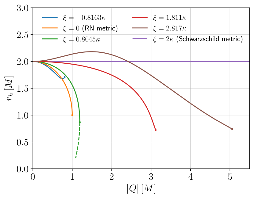
Figure 1: Radius of the event horizon $r_{h}$ versus bumblebee charge $Q$ of the black hole. Except for $\xi=2\kappa$, a maximally charged black-hole solution, indicated by a solid dot on each line, exists for a given coupling constant $\xi$. Notice that for the green line with $\xi=0.8045\kappa$, the bumblebee charge $Q$ turns back after reaching its maximum.

By specifying suitable values for $r_{h}$ and the limit of $(r-r_{h})\,g_{rr}$ at $r\rightarrow r_{h}$, we obtain black-hole solutions by integrating the field equations outward. The mass $M$ and the charge $Q$ for each solution can then be extracted according to Eq. (7). Using the mass $M$ as the unit, the radius of the event horizon $r_{h}$ with respect to the charge $Q$ is plotted in Fig. 1, for different values of the coupling constant $\xi$. As expected, the numerical solutions recover the Reissner-Nordström solution when $\xi=0$. What remarkable is that when $\xi=2\kappa$, the metric of the numerical solutions becomes the Schwarzschild metric, independent of the bumblebee charge which therefore can be arbitrarily large. In this case, $b_{t}$ also has an interesting analytic expression, $b_{t}\propto 1-2M/r$. We also notice that when $\xi>0$, the maximal charge-mass ratio for the black hole is larger than unity. Finally, let us point out that when $\xi$ is between 0 and about $1.2\kappa$, two black-hole solutions exist given a value of $Q$ near the maximal charge (see the green curve with a dashed segment in Fig. 1). We suspect the one with the smaller $r_{h}$ to be unstable and drop these solutions in the following analysis though further stability study is needed to confirm the speculation.

To have a view of the existence domain for the black-hole solutions, we still use the mass of the black hole as the unit, and generate in Fig. 2 a contour plot representing different value levels for the radius of the event horizon on the two-dimensional plane of the coupling constant $\xi$ and the bumblebee charge $Q$. The boundary of the contour plot indicates the change of the maximal charge-mass ratio with respect to the coupling constant $\xi$, namely that black-hole solutions do not exist in the blank region. Notice that $r_{h}$ does not approach zero at the boundary of the existence domain. Excluding the suspected unstable solutions corresponding to the dashed segment in Fig. 1, the minimal radius of the event horizon for all values of $\xi$ is above $0.7M$. At $\xi=2\kappa$, the metric takes the form of the Schwarzschild solution with $r_{h}=2M$ regardless of the bumblebee charge $Q$ which can be arbitrarily large. As $\xi$ goes away from the special value $\xi=2\kappa$, the maximal charge-mass ratio decreases rapidly.

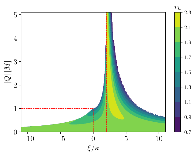
Figure 2: Contour plot for the radius of the event horizon $r_{h}$ on the $\xi$-$Q$ plane with the mass of the black hole being the unit of $r_{h}$ and $Q$. The red dashed lines indicate $\xi=0$ and $\xi=2\kappa$. The uneven boundary on the right part of the plot is due to numerical difficulties in finding the maximally charged black-hole solutions when $\xi$ is large.

3 Constraints from the EHT observations.

The EHT Collaboration successfully constructed shadow images for the supermassive black holes in the centers of the galaxy M87 (Akiyama et al., 2019) and the Milky Way (Akiyama et al., 2022a), providing quantitive evidences for the scale of black-hole event horizon. When alternatives to GR predict black holes with different sizes of event horizon, the shadow images can be used to test and constrain them. As the shadow of a black hole is casted when the EM waves emitted by matter near the event horizon are absorbed by the black hole, the exact size and shape of the shadow depend not only on the size of the event horizon but also on the distribution and the motion of matter around the black hole. The effect due to matter is complicated, but generally small when considering its correction to the size of the shadow, given current observational uncertainties of the masses and distances of the two supermassive black holes (Akiyama et al., 2019, 2022a). Therefore, we neglect the effect due to matter in this work but acknowledge that modelling matter surrounding the black hole is highly demanded for improving the test as well as explaining image details.

Without concerning the distribution and the motion of matter around a black hole, the shadow of the black hole is determined by the trajectory of the light that barely escapes from the light ring near the event horizon. For an observer far away from the black hole, the radius of the shadow is the distance between the line of sight and the approaching trajectory of the light, which is equivalently the impact parameter for the scattering lightlike geodesic that infinitely orbits around the light ring. In the spacetime described by the metric in Eq. (4), lightlike geodesics have four-velocity components

$$\frac{dt}{d\lambda}=e^{-2\nu},$$

$$\frac{dr}{d\lambda}=\pm e^{-\mu}\sqrt{e^{-2\nu}-\frac{\sigma^{2}}{r^{2}}},$$

$$\frac{d\theta}{d\lambda}=0,$$

$$\frac{d\phi}{d\lambda}=\frac{\sigma}{r^{2}},$$ (8)

where $\lambda$ is an affine parameter, $\sigma$ is an integral constant, and spherical symmetry has been used to put the orbit in the equatorial plane. To see that $\sigma$ is the impact parameter for scattering orbits, we take the $x$-axis along the velocity direction of the orbit at infinity. Then, as $r$ goes to infinity, we have $\phi\rightarrow 0$, and the impact parameter is

$$\lim\limits_{r\rightarrow\infty}r\phi=\lim\limits_{r\rightarrow\infty}r^{2}\times\frac{\big{|}{d\phi}/{d\lambda}\big{|}}{\big{|}{dr}/{d\lambda}\big{|}}=\sigma\lim\limits_{r\rightarrow\infty}e^{\mu+\nu}.$$ (9)

The black-hole solutions to be tested here are asymptotically flat, so $\sigma$ is the impact parameter.

The value of the impact parameter $\sigma$ on the light ring gives the radius of the black-hole shadow. It can be computed using the definition of the light ring, namely

$$\frac{dr}{d\lambda}=0,\quad\frac{d^{2}r}{d\lambda^{2}}=0.$$ (10)

The $r$-component of the four-acceleration can be obtained from the geodesic equations. After some simplification, Eq. (10) gives

$$re^{-\nu}=\sigma,\quad r\nu^{\prime}=1,$$ (11)

where the prime denotes the derivative with respect to $r$. Our numerical solutions are interpolated to solve the radius of the light ring, denoted as $r_{\rm lr}$, from the second equation in Eq. (11). Then using $r_{\rm lr}$, the first equation in Eq. (11) gives the value of $\sigma$ for the light ring, denoted as $\sigma_{\rm lr}$, which is the radius of the shadow for nonspinning black holes. The spin of a black hole causes small distortion to the shape of the black-hole shadow in GR, correcting deduced parameters by factors of order unity (Akiyama et al., 2022b, c). We do not know if the same is true in bumblebee gravity as rigorous solutions of rotating black holes in the bumblebee theory have not been found to our knowledge. Though it is beyond the scope of the present work, constructing solutions of rotating black holes and putting them into test would be worthwhile as the resolution of EHT improves.

For observational results, we have an angular diameter $d=42\pm 3\,\mu{\rm as}$ for the shadow of the black hole in M87 (Akiyama et al., 2019), and an angular diameter $d=51.8\pm 2.3\,\mu{\rm as}$ for the shadow of the black hole in the Milky Way (Akiyama et al., 2022a). As the angular diameter is related to the radius $\sigma_{\rm lr}$ by

$$d=\frac{2\sigma_{\rm lr}}{D}=\frac{2\sigma_{\rm lr}}{M}\frac{M}{D},$$ (12)

where $M$ and $D$ are the mass and distance of the black hole, the mass-distance ratio is required to obtain the observational value of $\sigma_{\rm lr}$ in unit of the black hole mass. For the supermassive black hole in M87, we adopt $M/D=3.62\pm 0.60\,\mu{\rm as}$ from stellar dynamics (Gebhardt et al., 2011), and for the supermassive black hole in the Milky Way, we adopt the average of the results from the Very Large Telescope Interferometer (Abuter et al., 2022) and Keck (Do et al., 2019) while their difference is used as the uncertainty, namely $M/D=5.02\pm 0.20\,\mu{\rm as}$. In conclusion, we have

$$\frac{\sigma_{\rm lr}}{M}=5.80\pm 1.05$$ (13)

for the supermassive black hole in M87, and

$$\frac{\sigma_{\rm lr}}{M}=5.16\pm 0.31$$ (14)

for the supermassive black hole in the Milky Way. Figure 3 shows the region on the $\xi$-$Q$ plane for the bumblebee black holes that are consistent with the results in Eqs. (13) and (14).

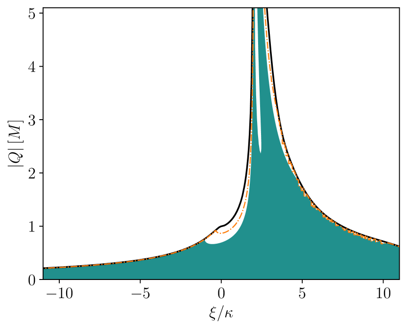
Figure 3: Constraints on the $\xi$-$Q$ plane due to the observations of the shadows for the supermassive black holes in M87 and the Milky Way. The shaded region is generated by letting numerically calculated $\sigma_{\rm lr}/M$ to satisfy the upper and lower bounds from Sgr A* in Eq. (14). The dash-dotted orange line is by satisfying the lower bound in Eq. (13) while the upper bound in Eq. (13) is trivially satisfied by all the solutions. The solid black line is the smoothed boundary of the plot in Fig. 2, indicating the existence domain of the black-hole solutions.

4 Conclusions.

In this work, we have presented black-hole solutions in the bumblebee gravity model described by the action in Eq. (1). The coupling between the bumblebee vector field and the Ricci tensor enriches the content of the theory, leading to two families of black-hole solutions. One extends the Reissner-Nordström solution in the Einstein-Maxwell theory, and the other appears to generalize the Schwarzschild solution for nonzero coupling constant $\xi$. As the metric of the solution in the latter family has been constrained very close to the Schwarzschild metric regardless of the bumblebee field (Xu et al., 2023), we have only considered testing solutions in the first family in this work.

Using astronomical observations on the shadows and the mass-distance ratios of two supermassive black holes, we have identified the region for the bumblebee black holes that are consistent with the observations on the two-dimensional plane of the coupling constant $\xi$ and the bumblebee charge $Q$ as shown in Fig. 3. The parameter space is only moderately constrained. We attribute this to two features in the solutions of the bumblebee model. First, we find that the metric of the black-hole solution is exactly the Schwarzschild metric while the bumblebee charge can be arbitrarily large if $\xi=2\kappa$. Thus for $\xi\sim 2\kappa$, the metric is too close to the Schwarzschild metric for the bumblebee charge to be constrained by the black-hole shadow observations. Second, for large $|\xi|$, the maximal bumblebee charge that a black hole can carry is automatically suppressed in the solution, so the metric is expected to be close to the Schwarzschild metric anyway. Therefore little parameter space is excluded for large $|\xi|$ too.

From another point of view, the difficulty in distinguishing a bumblebee black hole from the Schwarzschild black hole in GR using the observations of black-hole shadows indicates how capable an alternative to GR the bumblebee model is. To discriminate between GR and the bumblebee model, state-of-the-art techniques of multimessenger and multiwavelength astronomy are desirable, especially observations of GWs and X-rays that encode complementary information about gravity around black holes in addtion to the radio images from EHT. Features of GW polarizations in the bumblebee model that are very different from those in GR have recently been found in Liang et al. (2022a), and an estimate of constraints using future observations of extrem mass ratio inspirals (EMRIs) has been carried out in Liang et al. (2022b). Further work on finding modifications to GWs emitted in coalescences of stellar-mass black holes would be the next step for putting the bumblebee model into test against GW observations. Observations of X-rays from accretion disks of astrophysical black holes also provide exciting opportunities to test black hole spacetime metric. In fact, the spectral analysis techniques of X-rays are now mature enough to give even slightly better constraints on alternative black-hole solutions than those from GWs when elaborate accretion models are set up and suitable sources are carefully chosen as shown in Tripathi et al. (2021) and Bambi (2022). As the current package for analyzing X-ray data from black-hole accretion disks requires analytical spacetime metric solutions (Bambi, 2022), it would be necessary to incorporate algorithms that can use numerical metric solutions into the package to test the numerical bumblebee black holes in the future. In the meanwhile, with the next generation EHT (ngEHT) and space-borne sub-millimeter interferometries (Blackburn et al., 2019; Gurvits et al., 2022), sharper black hole images are on the way. A combination of the ngEHT images with X-ray and GW observations will eventually provide a more complete landscape for bumblebee-like vector-tensor gravity theories.

References

- Abbott et al. (2019) Abbott, B. P., et al. 2019, Phys. Rev. X, 9, 031040, doi: 10.1103/PhysRevX.9.031040
- Abbott et al. (2021a) Abbott, R., et al. 2021a, Phys. Rev. X, 11, 021053, doi: 10.1103/PhysRevX.11.021053
- Abbott et al. (2021b) —. 2021b. https://arxiv.org/abs/2111.03606
- Abuter et al. (2022) Abuter, R., et al. 2022, Astron. Astrophys., 657, L12, doi: 10.1051/0004-6361/202142465
- Akiyama et al. (2019) Akiyama, K., et al. 2019, Astrophys. J. Lett., 875, L1, doi: 10.3847/2041-8213/ab0ec7
- Akiyama et al. (2022a) —. 2022a, Astrophys. J. Lett., 930, L12, doi: 10.3847/2041-8213/ac6674
- Akiyama et al. (2022b) —. 2022b, Astrophys. J. Lett., 930, L15, doi: 10.3847/2041-8213/ac6736
- Akiyama et al. (2022c) —. 2022c, Astrophys. J. Lett., 930, L16, doi: 10.3847/2041-8213/ac6672
- Bailey & Kostelecký (2006) Bailey, Q. G., & Kostelecký, V. A. 2006, Phys. Rev. D, 74, 045001, doi: 10.1103/PhysRevD.74.045001
- Bambi (2022) Bambi, C. 2022. https://arxiv.org/abs/2210.05322
- Blackburn et al. (2019) Blackburn, L., et al. 2019. https://arxiv.org/abs/1909.01411
- Bluhm (2006) Bluhm, R. 2006, Lect. Notes Phys., 702, 191, doi: 10.1007/3-540-34523-X_8
- Bluhm et al. (2008a) Bluhm, R., Fung, S.-H., & Kostelecký, V. A. 2008a, Phys. Rev. D, 77, 065020, doi: 10.1103/PhysRevD.77.065020
- Bluhm et al. (2008b) Bluhm, R., Gagne, N. L., Potting, R., & Vrublevskis, A. 2008b, Phys. Rev. D, 77, 125007, doi: 10.1103/PhysRevD.79.029902
- Bluhm & Kostelecký (2005) Bluhm, R., & Kostelecký, V. A. 2005, Phys. Rev. D, 71, 065008, doi: 10.1103/PhysRevD.71.065008
- Casana et al. (2018) Casana, R., Cavalcante, A., Poulis, F. P., & Santos, E. B. 2018, Phys. Rev. D, 97, 104001, doi: 10.1103/PhysRevD.97.104001
- Colladay & Kostelecký (1997) Colladay, D., & Kostelecký, V. A. 1997, Phys. Rev. D, 55, 6760, doi: 10.1103/PhysRevD.55.6760
- Colladay & Kostelecký (1998) —. 1998, Phys. Rev. D, 58, 116002, doi: 10.1103/PhysRevD.58.116002
- Do et al. (2019) Do, T., et al. 2019, Science, 365, 664, doi: 10.1126/science.aav8137
- Gebhardt et al. (2011) Gebhardt, K., Adams, J., Richstone, D., et al. 2011, Astrophys. J., 729, 119, doi: 10.1088/0004-637X/729/2/119
- Gurvits et al. (2022) Gurvits, L. I., et al. 2022, Acta Astronaut., 196, 314, doi: 10.1016/j.actaastro.2022.04.020
- Kostelecký (2004) Kostelecký, V. A. 2004, Phys. Rev. D, 69, 105009, doi: 10.1103/PhysRevD.69.105009
- Kostelecký & Li (2019) Kostelecký, V. A., & Li, Z. 2019, Phys. Rev. D, 99, 056016, doi: 10.1103/PhysRevD.99.056016
- Kostelecký & Mewes (2009) Kostelecký, V. A., & Mewes, M. 2009, Phys. Rev. D, 80, 015020, doi: 10.1103/PhysRevD.80.015020
- Kostelecký & Mewes (2012) —. 2012, Phys. Rev. D, 85, 096005, doi: 10.1103/PhysRevD.85.096005
- Kostelecký & Mewes (2013) —. 2013, Phys. Rev. D, 88, 096006, doi: 10.1103/PhysRevD.88.096006
- Kostelecký & Russell (2011) Kostelecký, V. A., & Russell, N. 2011, Rev. Mod. Phys., 83, 11, doi: 10.1103/RevModPhys.83.11
- Liang et al. (2022a) Liang, D., Xu, R., Lu, X., & Shao, L. 2022a, Phys. Rev. D, 106, 124019, doi: 10.1103/PhysRevD.106.124019
- Liang et al. (2022b) Liang, D., Xu, R., Mai, Z.-F., & Shao, L. 2022b. https://arxiv.org/abs/2212.09346
- Tasson (2016) Tasson, J. D. 2016, Symmetry, 8, 111, doi: 10.3390/sym8110111
- Tripathi et al. (2021) Tripathi, A., Zhang, Y., Abdikamalov, A. B., et al. 2021, Astrophys. J., 913, 79, doi: 10.3847/1538-4357/abf6cd
- Xu (2023) Xu, R. 2023, in 9th Meeting on CPT and Lorentz Symmetry. https://arxiv.org/abs/2301.12666
- Xu et al. (2023) Xu, R., Liang, D., & Shao, L. 2023, Phys. Rev. D, 107, 024011, doi: 10.1103/PhysRevD.107.024011