Hurwitz numbers for reflection groups $B$ and $D$

Abstract.

We are building a theory of simple Hurwitz numbers for the reflection groups B and D parallel to the classical theory for the symmetric group. We also study analogs of the cut-and-join operators. An algebraic description of Hurwitz numbers and an explicit formula for them in terms of Schur polynomials are provided. We also relate Hurwitz numbers for B and D to ribbon decomposition of surfaces with boundary — a similar result for the symmetric group was proved earlier by Yu.Burman and the author. Finally, the generating function of B-Hurwitz numbers is shown to give rise to two independent $\tau$-function of the KP hierarchy.

Introduction

Hurwitz numbers are a classical topic in combinatorics and algebraic geometry; they date back to the work by Adolf Hurwtiz [7] (1890). A classical definition of the Hurwitz number $h_{m,\lambda}$ where $m$ is a non-negative integer and $\lambda=(\lambda_{1}\geq\dots\geq\lambda_{s})$ is a partition, is: $h_{m,\lambda}$ is the number of sequences of $m$ transpositions $(\sigma_{1},\dots,\sigma_{m})$ such that their product $\sigma_{1}\circ\dots\circ\sigma_{m}$ belongs to a conjugacy class $C_{\lambda}\in S_{n}$ in the symmetric group $S_{n}$. By a classical result [5], generating function of the Hurwitz numbers satisfies a second order parabolic PDE called the cut-and-join equation. Its right-hand side has Schur polynomials as eigenvectors, so the Hurwitz numbers can be expressed via them [10]. The result by A. Okounkov about Toda lattice [14] implies that the same generating function is a solution of the KP hierarchy (the proof uses tools coming from mathematical physics, namely the boson-fermion correspondence). Finally, in a recent work [1] by Yu.Burman and the author Hurwitz numbers are shown to solve a problem in low-dimensional topology: they are the numbers of ways to glue $m$ ribbons to a collection of $n$ disks so as to obtain a surface with a prescribed structure of the boundary.

In this paper we show that there is a parallel theory of Hurwitz numbers for the reflection groups of series B and D. Section 1 is the starting point where we recall the classical embedding of $B_{n}$ and $D_{n}$ into the symmetric group $S_{2n}$; the reflections are mapped to transpositions and products of pairs of transpositions commuting with the involution $\tau=(1,n+1)(2,n+2)\dots(n,2n)$ (for the group $D_{n}$, only pairs of transpositions are used). Also we recall a description of the conjugacy classes in these groups, taken from [3] (see Proposition 1.4; the classes are generally indexed by pairs of partitions $\lambda$ and $\mu$ such that $\left|\smash{\lambda}\right|\vphantom{\lambda}+\left|\smash{\mu}\right|\vphantom{\mu}=n$).

Section 2 gives the actual definition of Hurwitz numbers for the groups $B_{n}$ and $D_{n}$: it is similar to the classical one with reflections instead of transpositions. For the B series, we count reflections of two classes (transpositions and pairs of transpositions) separately.

In Sections 3 and 4 we study how the multiplication by a reflection affects conjugacy classes; this gives us an expression for the cut-and-join operator for the groups of series B and D. After a suitable change of variables we see that the operator obtained for the B group is actually a tensor square of the classical cut-and-join. The cut-and-join for the D group is a direct sum of the cut-and-join for B and the classical cut-and-join rescaled. This leads to an expression of the Hurwitz numbers for B and D via Schur polynomials.

In Section 5.1 we provides a model for B-Hurwitz numbers involving ribbon decomposition of surfaces equipped with an involution. Finally, in Section 5.2 we apply the boson-fermion correspondence to the tensor square of the cut-and-join described above; it allows one to show that the generating function of the B-Hurwitz numbers is a $2$-parameter family of $\tau$-functions of the KP hierarchy, independently in $2$ variables, and to prove a similar result for D.

Acknowledgements

The author wants to thank his advisor Yurii Burman for many fruitful discussions and constant attention to this work.

The research was partially funded by the HSE University Basic Research Program and by the International Laboratory of Cluster Geometry NRU HSE (RF Government grant, ag. No. 075-15-2021-608 dated 08.06.2021)

1. Reflection groups $B_{n}$ and $D_{n}$

1.1. Definition and embedding into $S_{2n}$

Let $B_{n}$ be a rank $n$ finite reflection group with the mirrors $x_{i}-x_{j}=0$, $x_{i}+x_{j}=0$ ($1\leq i<j\leq n$) and $x_{i}=0$ ($1\leq i\leq n$); the corresponding reflections are denoted $s_{ij}^{+}$, $s_{ij}^{-}$, and $\ell_{i}$, respectively (see [6] for details and standard notation). The subgroup $D_{n}\subset B_{n}$ is generated by $s_{ij}^{\pm}$ only.

Consider an involution $\tau\in S_{2n}$ without fixed points. All such involutions are conjugate, and the results that follow do not depend on a particulate choice; still, fix $\tau\stackrel{{\scriptstyle\mbox{\tiny def}}}{{=}}(1,n+1)(2,n+2)\dots(n,2n)$ (that is, $\tau(i)=i+n\bmod 2n$ for all $i$).

Groups $B_{n}$ and $D_{n}$ admit embedding into the permutation group $S_{2n}$. Namely,

Proposition 1.1.

There exists an embedding $\Phi:B_{n}\to S_{2n}$ such that $\Phi(s_{ij}^{+})=(ij)(i+n,j+n)$, $\Phi(s_{ij}^{-})=(i,j+n)(i+n,j)$ and $\Phi(\ell_{i})=(i,i+n)$. The image $\Phi(B_{n})$ is the normalizer of $\tau$:

$$\Phi(B_{n})=\{\sigma\in S_{2n}\mid\sigma\tau=\tau\sigma\}\stackrel{{\scriptstyle\mbox{\tiny def}}}{{=}}\operatorname{\mathrm{Norm}}(\tau),$$

and the image of the subgroup $D_{n}\subset B_{n}$ under $\Phi$ is the intersection of $\operatorname{\mathrm{Norm}}(\tau)$ with group $S_{2n}^{+}\subset S_{2n}$ of even permutations.

Introduce a notation more convenient for our purposes: let $r_{ij}\stackrel{{\scriptstyle\mbox{\tiny def}}}{{=}}(i,j)(i+n,j+n)$ for all $1\leq i\neq j\leq 2n$, $i\neq j\pm n$; addition is modulo $2n$. So if $1\leq i<j\leq n$ then $r_{ij}=r_{i+n,j+n}=\Phi(s_{ij}^{+})$ and $r_{i,j+n}=r_{i+n,j}=\Phi(s_{ij}^{-})$. Also denote $l_{i}\stackrel{{\scriptstyle\mbox{\tiny def}}}{{=}}(i,i+n)$ for all $1\leq i\leq 2n$; so, $l_{i}=l_{i+n}=\Phi(\ell_{i})$ if $i\leq n$.

A proof (rather elementary) of Proposition 1.1 is preceded by an explicit description of $\operatorname{\mathrm{Norm}}(\tau)$, which will be used extensively throughout this article:

Lemma 1.2.

If $x\in\operatorname{\mathrm{Norm}}(\tau)$ then for every cycle $(\gamma_{1}\dots\gamma_{m})$ of its cycle decomposition one of the following is true:

1. The cycle decomposition contains another cycle $(\gamma_{1}^{\prime}\dots\gamma_{m}^{\prime})$ of the same length such that $\gamma_{i}^{\prime}=\tau(\gamma_{i})$ for $i=1,\dots,s$.

2. $s=2t$ is even and $\gamma_{i+t}=\tau(\gamma_{i})$ for all $i=1,\dots,t$.

In the two cases we speak about $\alpha$-pairs of cycles and about $\beta$-cycles, respectively.

Proof.

Let

$$x=(\gamma_{11}\dots\gamma_{1m_{1}})\dots(\gamma_{q1}\dots\gamma_{qm_{q}})$$

be the cycle decomposition. If $\tau x=x\tau$ then $\tau x\tau^{-1}=x$. So

$$x=(\tau(\gamma_{11})\dots\tau(\gamma_{1m_{1}}))\dots(\tau(\gamma_{q1})\dots\tau(\gamma_{qm_{q}}))$$

The cycle decomposition is unique, so every cycle $(\tau(\gamma_{i1})\dots\tau(\gamma_{im_{i}}))$ must be equal to some $(\gamma_{j_{1}}\dots\gamma_{jm_{j}})$. If these two cycles are different, then they form an $\alpha$-pair. If these two cycles are the same then there exists some $t$ such that $\tau(\gamma_{k})=\gamma_{k+t\bmod m_{i}}$ for all $k=1,\dots,m_{i}$. Since $\tau$ is an involution, one has $\gamma_{k}=\tau^{2}(\gamma_{i})=\tau(\gamma_{k+t\bmod m_{i}})=\gamma_{k+2t\bmod m_{i}}$ for all $k=1,\dots,m_{i}$, which implies $m_{i}=2t$, and this is a $\beta$-cycle. ∎

Proof of Proposition 1.1.

Any element $x\in B_{n}$ is representable as $x=a_{1}\dots a_{N}$ where every $a_{k}$ is a reflection. Denote by $e_{1},\dots,e_{n}$ the standard basis in $\mathbb{R}^{n}$.

Lemma 1.3.

For any $k=1,\dots,n$ one has $x(e_{k})=\pm e_{\ell}$ for some $\ell=1,\dots,n$. If $x(e_{k})=e_{\ell}$ then $(\tilde{a}_{1}\tilde{}\dots\tilde{a}_{N})(k)=\ell$, and if $x(e_{k})=-e_{\ell}$ then $(\tilde{a}_{1}\tilde{}\dots\tilde{a}_{N})(k)=\tau(\ell)(=\ell+n)$.

The lemma is proved by an immediate induction by $N$.

Let us define now the map $\Phi:B_{n}\to S_{2n}$ as $\Phi(x)=\tilde{a}_{1}\dots\tilde{a}_{N}$. If $x=b_{1}\dots b_{M}$ is another representation of $x$ as a product of reflections, then Lemma 1.3 implies that $(\tilde{b}_{1}\dots\tilde{b}_{M})(k)=(\tilde{a}_{1}\dots\tilde{a}_{N})(k)$ for every $k$. Thus, the map $\Phi$ is well-defined and is a group homomorphism.

Suppose $\Phi(x)=\operatorname{\mathrm{id}}$ (that is, $x$ belongs to the kernel of $\Phi$). Then $(\tilde{a}_{1}\dots\tilde{a}_{N})(k)=k$ for every $k=1,\dots,n$, and Lemma 1.3 asserts then that $x(e_{k})=e_{k}$ for every $k$. Thus, $x=\operatorname{\mathrm{id}}$, so $\Phi$ is an embedding.

Show now that $\Phi(B_{n})=\operatorname{\mathrm{Norm}}(\tau)$. Obviously, $\Phi(B_{n})\subset\operatorname{\mathrm{Norm}}(\tau)$ because $\Phi(s^{\pm}_{ij})$ and $\Phi(\ell_{i})$ commute with $\tau$. Also, $\Phi(D_{n})\subset S_{2n}^{+}$ because $r_{ij}\in S_{2n}^{+}$.

Prove now that $\operatorname{\mathrm{Norm}}(\tau)\subset\Phi(B_{n})$. Let $x\in\operatorname{\mathrm{Norm}}(\tau)$. By Lemma 1.2, $x$ is a product of $\alpha$-pairs and of $\beta$-cycles, so to prove that $x\in\Phi(B_{n})$ it suffices to show that any $\alpha$-pair and any $\beta$-cycle are products of the elements $r_{ij}$ and $l_{i}$ ($1\leq i<j\leq 2n$). This is the case:

$$(i_{1},\dots,i_{m})(\tau(i_{1}),\dots,\tau(i_{m}))=r_{i_{1}i_{2}}\dots r_{i_{m-1}i_{m}}$$

and

$$(i_{1},\dots,i_{m}\tau(i_{1}),\dots,\tau(i_{m})) =(i_{1},\dots,i_{m})(\tau(i_{1}),\dots,\tau(i_{m}))(i_{1}\tau(i_{1}))$$

$$=r_{i_{1}i_{2}}\dots r_{i_{m-1}i_{m}}l_{i_{1}}.$$

To prove that $\operatorname{\mathrm{Norm}}(\tau)\cap S_{2n}^{+}\subset\Phi(D_{n})$ observe that the element $x\in\operatorname{\mathrm{Norm}}(\tau)$ is even if and only it contains an even number of $\beta$-cycles. (Indeed, an $\alpha$-pair is always an even permutation, while a $\beta$-cycle is odd because its length is even.) So it suffices to prove that the product of any two $\beta$-cycles is a product of $r_{ij}$ (for $\alpha$-cycles if was proved above). Indeed,

$$(i_{1}\dots i_{m}\tau(i_{1}) \dots\tau(i_{m}))(j_{1}\dots i_{q}\tau(j_{1})\dots\tau(j_{q}))$$

$$=(i_{1}\dots i_{m})(\tau(i_{1})\dots\tau(i_{m}))(j_{1}\dots i_{q})(\tau(j_{1})\dots\tau(j_{q}))(i_{1}\tau(i_{1}))(j_{1}\tau(j_{1})).$$

The product of the first four cycles is already proved to be a product of $r_{ij}$, while for the two remaining cycles one has

$$(i_{1}\tau(i_{1}))(j_{1}\tau(j_{1}))=r_{ij}r_{i,\tau(j)}.$$

∎

To save space, below we will not distinguish $B_{n}$ and $D_{n}$ from their images $\Phi(B_{n}),\Phi(D_{n})\subset S_{2n}$.

1.2. Conjugacy classes

Conjugacy classes in the permutation group $S_{m}$ are in one-to-one correspondence with partitions of $m$: two elements of $S_{m}$ are conjugate if and only if they have cycles of the same lengths (totalling $m$) in their cycle decomposition. A similar result for the reflection groups $B_{n}$ and $D_{n}$ can be found in [3]. Quote it here for coompleteness; be warned that the original notation of [3] differ from the one used here.

Fix two partitions, $\lambda=(\lambda_{1},\dots,\lambda_{s})$ and $\mu=(\mu_{1},\dots,\mu_{t})$ such that $\left|\smash{\lambda}\right|\vphantom{\lambda}+\left|\smash{\mu}\right|\vphantom{\mu}=\lambda_{1}+\dots+\lambda_{s}+\mu_{1}+\dots+\mu_{t}=n$, and consider a set $C_{\lambda\mid\mu}$ of elements $x\in B_{n}\subset S_{2n}$ such that their cycle decomposition contains

1. $\alpha$-pairs of lengths (each cycle) $\lambda_{1},\lambda_{2},\dots,\lambda_{s}$;

2. $\beta$-cycles of lengths $2\mu_{1},\dots,2\mu_{t}$ (recall that the length should be even).

Proposition 1.4 ([3, Proposition 25]).

The set $C_{\lambda\mid\mu}\subset B_{n}$ is a conjugacy class. Every conjugacy class in $B_{n}$ is $C_{\lambda\mid\mu}$ for some $\lambda$ and $\mu$ such that $\left|\smash{\lambda}\right|\vphantom{\lambda}+\left|\smash{\mu}\right|\vphantom{\mu}=n$.

For $D_{n}$ the answer is slightly more complicated. Take a partition $\lambda=(\lambda_{1},\dots,\lambda_{s})$ such that $\left|\smash{\lambda}\right|\vphantom{\lambda}=n$ and all $\lambda_{i}$ are even. For an element $\sigma\in C_{\lambda\mid\emptyset}$ write its cycle decomposition

(1.1) $$\sigma=(\gamma_{11}\dots\gamma_{1\lambda_{1}})\dots(\gamma_{s1}\dots\gamma_{s\lambda_{s}})(\tau(\gamma_{11})\dots\tau(\gamma_{1\lambda_{1}}))\dots(\tau(\gamma_{s1})\dots\tau(\gamma_{s\lambda_{s}}))$$

satisfying two conditions: cycles forming an $\alpha$-pair always stand in position $i$ and $i+s$ in the cycle decomposition, and their matching elements $\gamma_{ij}$ and $\tau(\gamma_{ij})$ occupy the same positions in them. Now consider a permutation $\gamma=(\gamma_{11}\dots\gamma_{s\lambda_{s}})\in S_{2n}$ where the numbers $\gamma_{ij}$ are written exactly in the same order as in (1.1). We write $\sigma\in C_{\lambda\mid\emptyset}^{+}$ if $\gamma$ is even, and $\sigma\in C_{\lambda\mid\emptyset}^{-}$ if $\gamma$ is odd. Representation of $\sigma$ in the form (1.1) is not unique but, as it is easy to see, the parity of $\gamma$ does not depend on a particular choice. (Recall, all the cycles in (1.1) have even length.)

Proposition 1.5 ([3, Proposition 25]).

1. If the partition $\mu$ contains an even number of parts then the conjugacy class $C_{\lambda\mid\mu}\subset B_{n}$ lies in $D_{n}$; if the number of parts is odd then $C_{\lambda\mid\mu}$ does not intersect $D_{n}$.

2. If $\mu\neq\emptyset$ and the number of parts of $\mu$ is even then $C_{\lambda\mid\mu}$ is a conjugacy class in $D_{n}$.

3. If $\lambda$ is a partition of $n$ containing at least one odd part $\lambda_{i}$ then $C_{\lambda\mid\emptyset}$ is a conjugacy class in $D_{n}$.

4. If $\lambda$ is a partition of $n$ such that all its parts are even then $C_{\lambda\mid\emptyset}$ splits into two conjugacy classes in $D_{n}$, $C_{\lambda\mid\emptyset}^{+}$ and $C_{\lambda\mid\emptyset}^{-}$.

Any conjugacy class in $D_{n}$ is one of the classes listed above.

Corollary 1.6.

1. Let $\lambda,\mu$ be partitions such that $\left|\smash{\lambda}\right|\vphantom{\lambda}+\left|\smash{\mu}\right|\vphantom{\mu}=n$, $\#\mu$ is even and either $\mu\neq\emptyset$ or at least one of the parts of $\lambda$ is odd. Then for any $x\in B_{n}$ and any $\sigma\in C_{\lambda\mid\mu}\subset D_{n}$ one has $x\sigma x^{-1}\in C_{\lambda\mid\mu}$.

2. Let $\lambda$ be a partition of $n$ such that all its parts are even, and let $x\in B_{n}$. Then for any $\sigma\in C_{\lambda\mid\emptyset}^{+}$ one has $x\sigma x^{-1}\in C_{\lambda\mid\emptyset}^{+}$ if $x\in D_{n}\subset B_{n}$ (that is, $x\in S_{2n}$ is an even permutation) and $x\sigma x^{-1}\in C_{\lambda\mid\emptyset}^{-}$ otherwise; the picture for $\sigma\in C_{\lambda\mid\emptyset}^{-}$ is symmetric.

In particular, $C_{{1^{n-2}2^{1}}\mid\varnothing}\subset D_{n}\subset B_{n}$ consists of all the reflections $r_{ij}$, and $C_{{1^{n-1}}\mid 1}\subset B_{n}$, of all the reflections $l_{i}$.

2. Hurwitz numbers

2.1. Definitions

Fix a pair of partitions $\lambda,\mu$ with $\left|\smash{\lambda}\right|\vphantom{\lambda}+\left|\smash{\mu}\right|\vphantom{\mu}=n$. Let $C_{\lambda\mid\mu}\subset B_{n}$ be the conjugacy class defined above.

Definition 2.1.

A sequence of reflections $(\sigma_{1},\dots,\sigma_{m+\ell})$ of the group $B_{n}$ is said to have profile $(\lambda,\mu,m,\ell)$ if $\#\{p\mid\sigma_{p}=r_{ij},1\leq i<j\leq 2n\}=m$, $\#\{p\mid\sigma_{p}=l_{i},1\leq i\leq 2n\}=\ell$ and $\sigma_{1}\dots\sigma_{m+\ell}\in C_{\lambda\mid\mu}$. The Hurwitz numbers for the group $B_{n}$ are $h_{m,\ell,\lambda,\mu}^{B}=\frac{1}{n!}\#\{(\sigma_{1},\dots,\sigma_{m+\ell})\text{ is a sequence of profile }(\lambda,\mu,m,\ell)\}$.

For the group $D_{n}$ we use the same numbers, in case they make sense:

Definition 2.2.

Let $m$ be a positive integer, and $\lambda$ and $\mu$, partitions where the number of parts $\#\mu$ is even. The Hurwitz number for the group $D_{n}$ is defined as $h_{m,\lambda,\mu}^{D}=h_{m,0,\lambda,\mu}^{B}$.

In other words, $h_{m,\lambda,\mu}^{D}=\frac{1}{n!}\#\{(\sigma_{1},\dots,\sigma_{m})\text{ has profile }(\lambda,\mu,m)\}$ where $\sigma_{p}$ are reflections in the group $D_{n}$ (that is, $\sigma_{p}=r_{ij}$ for some $i$ and $j$), and the profile means that $\sigma_{1}\dots\sigma_{m}\in C_{\lambda\mid\mu}\subset D_{n}$.

Remark 2.3.

Recall (Proposition 1.5) that if $\mu=\emptyset$ and all the parts of the partition $\lambda$ are even then $C_{\lambda\mid\emptyset}$ splits into two conjugacy classes, $C_{\lambda\mid\emptyset}^{+}$ and $C_{\lambda\mid\emptyset}^{-}$.

Denote by $\Sigma_{m,\lambda}^{+}$ and $\Sigma_{m,\lambda}^{-}$ the sets of $m$-tuples of reflections $\sigma_{1},\dots,\sigma_{m}\in D_{n}$ such that $\sigma_{1}\dots\sigma_{m}\in C_{\lambda\mid\emptyset}^{+}$ (resp., $C_{\lambda\mid\emptyset}^{-}$). One can denote $h_{m,\lambda,\emptyset\pm}^{D}\stackrel{{\scriptstyle\mbox{\tiny def}}}{{=}}\frac{1}{n!}\#\Sigma_{m,\lambda}^{\pm}$, so that $h_{m,\lambda,\emptyset+}^{D}+h_{m,\lambda,\emptyset-}^{D}=h_{m,\lambda,\emptyset}^{D}$. It follows from Corollary 1.6, though, that if $x\in B_{n}$ but $x\notin D_{n}$ then the map sending an $m$-tuple $(\sigma_{1},\dots,\sigma_{m})$ to $(x\sigma_{1}x^{-1},\dots,x\sigma_{m}x^{-1})$ is a bijection between $\Sigma_{m,\lambda}^{+}$ and $\Sigma_{m,\lambda}^{-}$. Thus, $h_{m,\lambda,\emptyset+}^{D}=h_{m,\lambda,\emptyset-}^{D}=\frac{1}{2}h_{m,\lambda,\emptyset}^{D}$, so considering $h_{m,\lambda,\emptyset\pm}^{D}$ makes little sense.

Up to the end of this section we consider the Hurwitz numbers for the group $B_{n}$ only.

Denote by $\operatorname{\mathcal{C}}\nolimits_{\lambda\mid\mu}\stackrel{{\scriptstyle\mbox{\tiny def}}}{{=}}\frac{1}{\#C_{\lambda\mid\mu}}\sum_{x\in C_{\lambda\mid\mu}}x\in\mathbb{C}[B_{n}]$ the normalized class sum. One has $\operatorname{\mathcal{C}}\nolimits_{\lambda\mid\mu}\in Z[B_{n}]$ (the center of the group algebra of $B_{n}$); by Proposition 1.4, $\operatorname{\mathcal{C}}\nolimits_{\lambda\mid\mu}$ form a basis in $Z[B_{n}]$. Consider now a ring of polynomials $\mathbb{C}[p,q]$ where $p=(p_{1},p_{2},\dots)$ and $q=(q_{1},q_{2},\dots)$ are two infinite sets of variables. The ring is graded by the total degree where one assumes $\deg p_{k}=\deg q_{k}=k$ for all $k=1,2,\dots$. The map $\Psi$ defined by

(2.1) $$\Psi(\operatorname{\mathcal{C}}\nolimits_{\lambda\mid\mu})=p_{\lambda}q_{\mu}\stackrel{{\scriptstyle\mbox{\tiny def}}}{{=}}p_{\lambda_{1}}\dots p_{\lambda_{s}}q_{\mu_{1}}\dots q_{\mu_{t}}$$

establishes an isomorphism between $Z[B_{n}]$ and the homogeneous component $\mathbb{C}[p,q]_{n}$ of total degree $n$.

Now denote by

(2.2) $$\mathcal{T}_{1}:=\frac{1}{2}\sum_{1\leq i<j\leq 2n}r_{ij}=\#C_{21^{n-2}\mid\emptyset}\cdot\operatorname{\mathcal{C}}\nolimits_{1^{n-2}2\mid\emptyset}$$

and

$$\mathcal{T}_{2}:=\frac{1}{2}\sum_{1\leq i\leq 2n}l_{i}=\#C_{1^{n-1}\mid 1}\cdot\operatorname{\mathcal{C}}\nolimits_{1^{n-1}\mid 1}$$

sums of all elements of the conjugacy classes containing reflections (recall that $r_{ij}=r_{i+n,j+n}$, and $l_{i}=l_{i+n}$, so every element is repeated twice in these sums; hence the factor $\frac{1}{2}$). The elements $\mathcal{T}_{1}$ and $\mathcal{T}_{2}$ belong to $Z[B_{n}]$, so one can consider linear operators $T_{1},T_{2}:Z[B_{n}]\to Z[B_{n}]$ of multiplication by $\mathcal{T}_{1}$ and $\mathcal{T}_{2}$, respectively. Obviously, $T_{1}$ and $T_{2}$ commute.

Consider now linear operators $\mathcal{CJ}_{1},\mathcal{CJ}_{2}:\mathbb{C}[p,q]_{n}\to\mathbb{C}[p,q]_{n}$ making the following diagrams commutative:

(2.3) $$\lx@xy@svg{\hbox{\raise 0.0pt\hbox{\kern 18.21884pt\hbox{\ignorespaces\ignorespaces\ignorespaces\hbox{\vtop{\kern 0.0pt\offinterlineskip\halign{\entry@#!@&&\entry@@#!@\cr&\\&\crcr}}}\ignorespaces{\hbox{\kern-15.27267pt\raise 0.0pt\hbox{\hbox{\kern 0.0pt\raise 0.0pt\hbox{\hbox{\kern 3.0pt\raise 0.0pt\hbox{$\textstyle{Z[B_{n}]\ignorespaces\ignorespaces\ignorespaces\ignorespaces\ignorespaces\ignorespaces\ignorespaces\ignorespaces}$}}}}}}}\ignorespaces\ignorespaces\ignorespaces\ignorespaces{}{\hbox{\lx@xy@droprule}}\ignorespaces\ignorespaces\ignorespaces{\hbox{\kern 21.27617pt\raise 6.0512pt\hbox{{}\hbox{\kern 0.0pt\raise 0.0pt\hbox{\hbox{\kern 3.0pt\hbox{\hbox{\kern 0.0pt\raise-1.73215pt\hbox{$\scriptstyle{\times T_{i}}$}}}\kern 3.0pt}}}}}}\ignorespaces{\hbox{\kern 45.16501pt\raise 0.0pt\hbox{\hbox{\kern 0.0pt\raise 0.0pt\hbox{\lx@xy@tip{1}\lx@xy@tip{-1}}}}}}{\hbox{\lx@xy@droprule}}{\hbox{\lx@xy@droprule}}\ignorespaces\ignorespaces\ignorespaces\ignorespaces{}{\hbox{\lx@xy@droprule}}\ignorespaces\ignorespaces\ignorespaces{\hbox{\kern 0.0pt\raise-20.0pt\hbox{{}\hbox{\kern 0.0pt\raise 0.0pt\hbox{\hbox{\kern 3.0pt\hbox{\hbox{\kern 0.0pt\raise-1.62312pt\hbox{$\scriptstyle{\simeq}$}}}\kern 3.0pt}}}}}}\ignorespaces{\hbox{\kern 0.0pt\raise-29.5pt\hbox{\hbox{\kern 0.0pt\raise 0.0pt\hbox{\lx@xy@tip{1}\lx@xy@tip{-1}}}}}}{\hbox{\lx@xy@droprule}}{\hbox{\lx@xy@droprule}}{\hbox{\kern 45.16501pt\raise 0.0pt\hbox{\hbox{\kern 0.0pt\raise 0.0pt\hbox{\hbox{\kern 3.0pt\raise 0.0pt\hbox{$\textstyle{Z[B_{n}]\ignorespaces\ignorespaces\ignorespaces\ignorespaces}$}}}}}}}\ignorespaces\ignorespaces\ignorespaces\ignorespaces{}{\hbox{\lx@xy@droprule}}\ignorespaces\ignorespaces\ignorespaces{\hbox{\kern 60.43768pt\raise-20.0pt\hbox{{}\hbox{\kern 0.0pt\raise 0.0pt\hbox{\hbox{\kern 3.0pt\hbox{\hbox{\kern 0.0pt\raise-1.62312pt\hbox{$\scriptstyle{\simeq}$}}}\kern 3.0pt}}}}}}\ignorespaces{\hbox{\kern 60.43768pt\raise-29.5pt\hbox{\hbox{\kern 0.0pt\raise 0.0pt\hbox{\lx@xy@tip{1}\lx@xy@tip{-1}}}}}}{\hbox{\lx@xy@droprule}}{\hbox{\lx@xy@droprule}}{\hbox{\kern-18.21884pt\raise-40.0pt\hbox{\hbox{\kern 0.0pt\raise 0.0pt\hbox{\hbox{\kern 3.0pt\raise 0.0pt\hbox{$\textstyle{\mathbb{C}[p,q]_{n}\ignorespaces\ignorespaces\ignorespaces\ignorespaces}$}}}}}}}\ignorespaces\ignorespaces\ignorespaces\ignorespaces{}{\hbox{\lx@xy@droprule}}\ignorespaces\ignorespaces\ignorespaces{\hbox{\kern 22.20343pt\raise-46.05118pt\hbox{{}\hbox{\kern 0.0pt\raise 0.0pt\hbox{\hbox{\kern 3.0pt\hbox{\hbox{\kern 0.0pt\raise-1.73215pt\hbox{$\scriptstyle{\mathcal{CJ}_{i}}$}}}\kern 3.0pt}}}}}}\ignorespaces{\hbox{\kern 42.21884pt\raise-40.0pt\hbox{\hbox{\kern 0.0pt\raise 0.0pt\hbox{\lx@xy@tip{1}\lx@xy@tip{-1}}}}}}{\hbox{\lx@xy@droprule}}{\hbox{\lx@xy@droprule}}{\hbox{\kern 42.21884pt\raise-40.0pt\hbox{\hbox{\kern 0.0pt\raise 0.0pt\hbox{\hbox{\kern 3.0pt\raise 0.0pt\hbox{$\textstyle{\mathbb{C}[p,q]_{n}}$}}}}}}}\ignorespaces}}}}\ignorespaces,\qquad i=1,2. \textstyle{Z[B_{n}]\ignorespaces\ignorespaces\ignorespaces\ignorespaces\ignorespaces\ignorespaces\ignorespaces\ignorespaces} \scriptstyle{\times T_{i}} \scriptstyle{\simeq} \textstyle{Z[B_{n}]\ignorespaces\ignorespaces\ignorespaces\ignorespaces} \scriptstyle{\simeq} \textstyle{\mathbb{C}[p,q]_{n}\ignorespaces\ignorespaces\ignorespaces\ignorespaces} \scriptstyle{\mathcal{CJ}_{i}} \textstyle{\mathbb{C}[p,q]_{n}} \textstyle{Z[B_{n}]\ignorespaces\ignorespaces\ignorespaces\ignorespaces\ignorespaces\ignorespaces\ignorespaces\ignorespaces} \scriptstyle{\times T_{i}} \scriptstyle{\simeq} \textstyle{Z[B_{n}]\ignorespaces\ignorespaces\ignorespaces\ignorespaces} \scriptstyle{\simeq} \textstyle{\mathbb{C}[p,q]_{n}\ignorespaces\ignorespaces\ignorespaces\ignorespaces} \scriptstyle{\mathcal{CJ}_{i}} \textstyle{\mathbb{C}[p,q]_{n}}$$

Let now $\lambda,\lambda^{\prime},\mu,\mu^{\prime}$ be partitions such that $\left|\smash{\lambda}\right|\vphantom{\lambda}+\left|\smash{\mu}\right|\vphantom{\mu}=\left|\smash{\lambda^{\prime}}\right|\vphantom{\lambda^{\prime}}+\left|\smash{\mu^{\prime}}\right|\vphantom{\mu^{\prime}}=n$. Take an element $\sigma_{*}\in C_{\lambda\mid\mu}$ and define the multiplicity $\langle\lambda,\mu\mid\lambda^{\prime},\mu^{\prime}\rangle_{1}$ as the number of reflections $u\in C_{2^{1}1^{n-2}\mid\varnothing}$ (that is, $u=r_{ij}$) such that $u\sigma_{*}\in C_{\lambda^{\prime}\mid\mu^{\prime}}$; the multiplicity $\langle\lambda,\mu\mid\lambda^{\prime},\mu^{\prime}\rangle_{2}$ is defined in the same way with $u\in C_{1^{n-1}\mid 1}$ (that is, $u=l_{i}$) instead.

Lemma 2.4.

Multiplicities do not depend on the choice of $\sigma_{*}$.

Proof.

Denote by $S_{1}(\sigma_{*};\lambda^{\prime},\mu^{\prime})\subset C_{1^{n-2}2^{1}\mid\emptyset}$ the set of reflections $u$ such that $u\sigma_{*}\in C_{\lambda^{\prime}\mid\mu^{\prime}}$. Take $\sigma^{\prime}=x\sigma_{*}x^{-1}\in C_{\lambda\mid\mu}$ where $x\in B_{n}$. If $u\in S(\sigma^{\prime};\lambda^{\prime},\mu^{\prime})$ then $u\sigma^{\prime}=ux\sigma_{*}x^{-1}=x((x^{-1}ux)\sigma_{*})x^{-1}\in C_{\lambda^{\prime}\mid\mu^{\prime}}$, which is equivalent to $(x^{-1}ux)\sigma_{*}\in C_{\lambda^{\prime}\mid\mu^{\prime}}$, that is, to $x^{-1}ux\in S(\sigma_{*};\lambda^{\prime},\mu^{\prime})$. Thus, conjugation $u\mapsto x^{-1}ux$ is a one-to-one map sending $S_{1}(\sigma^{\prime};\lambda^{\prime},\mu^{\prime})$ to $S_{1}(\sigma_{*};\lambda^{\prime},\mu^{\prime})$, and therefore these two sets contain the same number of elements $\langle\lambda,\mu\mid\lambda^{\prime},\mu^{\prime}\rangle_{1}$. The reasoning for the multiplicity $\langle\lambda,\mu\mid\lambda^{\prime},\mu^{\prime}\rangle_{2}$ is the same. ∎

Theorem 2.5.

$T_{i}\operatorname{\mathcal{C}}\nolimits_{\lambda\mid\mu}=\sum_{\lambda^{\prime},\mu^{\prime}}\langle\lambda,\mu\mid\lambda^{\prime},\mu^{\prime}\rangle_{i}\operatorname{\mathcal{C}}\nolimits_{\lambda^{\prime}\mid\mu^{\prime}}$ for $i=1,2$.

Proof.

(2.4) $$T_{1}\operatorname{\mathcal{C}}\nolimits_{\lambda\mid\mu}=\frac{1}{\#C_{\lambda\mid\mu}}\sum_{\sigma\in C_{\lambda\mid\mu}}T_{1}\sigma=\frac{1}{\#C_{\lambda\mid\mu}}\sum_{\sigma\in C_{\lambda\mid\mu}}\sum_{u\in C_{1^{n-2}2^{1}\mid\varnothing}}u\sigma.$$

It follows from Lemma 2.4 that (2.4) is an arithmetical mean of identical summands, so it is equal to each of them:

$$T_{1}\operatorname{\mathcal{C}}\nolimits_{\lambda\mid\mu}=\sum_{\lambda^{\prime},\mu^{\prime}}\sum_{\begin{subarray}{c}u\in C_{1^{n-2}2^{1}\mid\varnothing}\\ u\sigma_{*}\in C_{\lambda^{\prime}\mid\mu^{\prime}}\end{subarray}}u\sigma_{*}$$

for any fixed $\sigma_{*}\in C_{\lambda\mid\mu}$. Using Lemma 2.4 again, one obtains

$$T_{1}\operatorname{\mathcal{C}}\nolimits_{\lambda\mid\mu} =\sum_{\lambda^{\prime},\mu^{\prime}}\sum_{\begin{subarray}{c}u\in C_{1^{n-2}2^{1}\mid\varnothing}\\ u\sigma_{*}\in C_{\lambda^{\prime}\mid\mu^{\prime}}\end{subarray}}\frac{1}{\#C_{\lambda^{\prime}\mid\mu^{\prime}}}\sum_{\tau\in C_{\lambda^{\prime}\mid\mu^{\prime}}}\tau$$

$$=\sum_{\lambda^{\prime},\mu^{\prime}}\#(\{u\in C_{1^{n-2}2^{1}\mid\varnothing}:u\sigma_{*}\in C_{\lambda^{\prime}\mid\mu^{\prime}}\}\operatorname{\mathcal{C}}\nolimits_{\lambda^{\prime}\mid\mu^{\prime}}$$

$$=\sum_{\lambda^{\prime},\mu^{\prime}}\langle\lambda,\mu\mid\lambda^{\prime},\mu^{\prime}\rangle\operatorname{\mathcal{C}}\nolimits_{\lambda^{\prime}\mid\mu^{\prime}}.$$

The proof for $T_{2}$ is the same with $C_{1^{n-1}\mid 1}$ instead of $C_{1^{n-2}2^{1}\mid\varnothing}$. ∎

2.2. Generating function

Consider the following generating function for Hurwitz numbers of the group $B_{n}$:

$$\mathcal{H}^{B}(\beta,\gamma,p,q)=\sum_{m,\ell}\sum_{\lambda,\mu}\frac{h_{m,\ell,\lambda,\mu}^{B}}{m!\ell!}p_{\lambda}q_{\mu}\beta^{m}\gamma^{\ell}.$$

Theorem 2.6.

$\mathcal{H}^{B}$ satisfies the cut-and-join equations

(2.5) $$\frac{\partial\mathcal{H}^{B}}{\partial\beta}=\mathcal{CJ}_{1}(\mathcal{H}^{B})\quad\text{and}\quad\frac{\partial\mathcal{H}^{B}}{\partial\gamma}=\mathcal{CJ}_{2}(\mathcal{H}^{B})$$

Proof.

Fix a positive integer $n$ and denote by $\mathcal{H}_{n}$ a degree $n$ homogeneous component of $\mathcal{H}^{B}$. The cut-and-join operators preserve the degree, so $\mathcal{H}^{B}$ satisfies the cut-and-join equations if and only if $\mathcal{H}_{n}$ does (for each $n$).

Let $i$ be $1$ or $2$, and let

$$\mathcal{G}_{n}\stackrel{{\scriptstyle\mbox{\tiny def}}}{{=}}\sum_{m,\ell\geq 0}\sum_{\lambda,\mu:\mid\lambda\mid+\mid\mu\mid=n}\frac{n!h_{m,\ell,\lambda,\mu}^{B}}{m!\ell!}\operatorname{\mathcal{C}}\nolimits_{\lambda\mid\mu}\beta^{m}\gamma^{\ell}\in\mathbb{C}[B_{n}]$$

An elementary combinatorial reasoning gives

$$\mathcal{G}_{n}=\sum_{m\geq 0}\frac{\beta^{m}\gamma^{\ell}}{m!\ell!}T_{1}^{m}T_{2}^{\ell}(e_{n})$$

where $e_{n}\in B_{n}$ is the unit element. Clearly

$$T_{1}(\mathcal{G}_{n})=\sum_{m\geq 0}\frac{\beta^{m}\gamma^{\ell}}{m!\ell!}(T_{1})^{m+1}(e_{n})=\sum_{m\geq 1}\frac{\beta^{m-1}\gamma^{\ell}}{(m-1)!\ell!}(T_{1})^{m}(e_{n})=\frac{\partial\mathcal{G}_{n}}{\partial\beta}.$$

and, similarly, $T_{2}(\mathcal{G}_{n})=\frac{\partial\mathcal{G}_{n}}{\partial\gamma}$. Applying the isomorphism $\Psi$ one obtains $\Psi T_{1}(\mathcal{G}_{n})=\Psi(\frac{\partial\mathcal{G}_{n}}{\partial\beta})=\frac{\partial}{\partial\beta}\Psi(\mathcal{G}_{n})$. One has $\Psi(\mathcal{G}_{n})=\mathcal{H}_{n}$, hence $\frac{\partial}{\partial\beta}\Psi(\mathcal{G}_{n})=\frac{\partial\mathcal{H}_{n}}{\partial\beta}$; similarly, $\frac{\partial}{\partial\gamma}\Psi(\mathcal{G}_{n})=\frac{\partial\mathcal{H}_{n}}{\partial\gamma}$. By the definition of the cut-and-join operators, $\Psi T_{1}(\mathcal{G}_{n})=\mathcal{CJ}_{1}(\Psi(\mathcal{G}_{n}))=\mathcal{CJ}_{1}({\mathcal{H}_{n}})$ and the same for $T_{2}$ and $\mathcal{CJ}_{2}$. Equalities (2.5) follow. ∎

Corollary 2.7.

(2.6) $$\mathcal{H}^{B}(\beta,\gamma,p,q)=e^{\beta\mathcal{CJ}_{1}+\gamma\mathcal{CJ}_{2}}e^{p_{1}}$$

Proof.

It follows from Definition 2.1 that $h^{B}_{0,0,\lambda,\mu}=\frac{1}{n!}$ if $\lambda=1^{n}$ and $\mu=\emptyset$, and $h^{B}_{0,0,\lambda,\mu}=0$ otherwise. Thus $\mathcal{H}^{B}(0,0,p,q)=e^{p_{1}}$ and (2.6) follows from Theorem 2.6. ∎

3. Explicit formulas

3.1. Multiplication of an element $x\in B_{n}\subset S_{2n}$ by a reflection

Let $\omega\in S_{n}$ and $1\leq a<b\leq n$. The cycle structure of the product $\omega^{\prime}=(ab)\omega$ depend on the cyclic structure of $\omega$ and positions of $a$ and $b$ as follows. If $a$ and $b$ belong to the same cycle $(a,\dots,u,b,\dots,v)$ of $\omega$, then the cycle splits in $\omega^{\prime}$ into two: $(a,\dots,u)$ and $(b,\dots,v)$ (“a cut”). If $a$ and $b$ belong to different cycles then the opposite thing happens: they glue together in $\omega^{\prime}$ (“a join”). The cycles containing neither $a$ nor $b$ are the same for $\omega$ and $\omega^{\prime}$.

Let now $\omega\in B_{n}\subset S_{2n}$. The cyclic structure of $\omega^{\prime}=\sigma\omega$ where $\sigma$ is a reflection (i.e. $\sigma=r_{ab}=(ab)(a+n,b+n)$ (addition modulo $n$) for $1\leq a<b\leq 2n$, or $\sigma=l_{a}=(a,a+n)$ for $1\leq a\leq 2n$) depends on the cyclic structure of $\omega$ ($\alpha$-pairs and $\beta$-cycles) and the position of the points $a,b$ as shown in Table 1 below.

In this table, hexagons represent $\beta$-cycles and the pairs of triangles are $\alpha$-pairs; numbers inside denote the lengths of the cycles. The two-headed dashed arrows show the position of $a$ and $b$ of the reflection $\sigma$. The solid arrows join cyclic structures of $\omega$ and $\sigma\omega$ for $\sigma=r_{ab}$, and the empty arrows, for $\sigma=l_{a}$ (recall that $\sigma$ is an involution, so the arrows are two-headed). For example, the first diagram shows the multiplication by $(a,b)(\tau(a),\tau(b))$ of a pair of $\beta$-cycles containing $a$ and $b$, respectively.

The boxed number on the bottom left corner is the multiplicity $\langle\lambda,\mu\mid\lambda^{\prime},\mu^{\prime}\rangle$ between conjugacy classes containing $\omega$ and $\sigma\omega$.

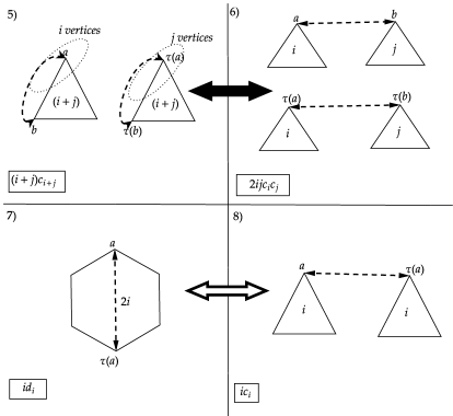
Figure 1. Multiplication of cycles by a reflection

3.2. Multiplicities

Let $\omega\in C_{\lambda\mid\mu}$ where $\lambda=1^{c_{1}}\dots n^{c_{n}}$ and $\mu=1^{d_{1}}\dots n^{d_{n}}$ — that is, for every $k=1,\dots,n$ the element $u$ contains $c_{k}$ $\alpha$-pairs of length $k$ and $d_{k}$ separate $\beta$-cycles of length $2k$. Calculate, for all $\lambda^{\prime}=1^{c_{1}^{\prime}}\dots n^{c_{n}^{\prime}}$ and $\mu=1^{d_{1}^{\prime}}\dots n^{d_{n}^{\prime}}$, the multiplicities $\langle\lambda^{\prime},\mu^{\prime}\mid\lambda,\mu\rangle_{1}$ and $\langle\lambda^{\prime},\mu^{\prime}\mid\lambda,\mu\rangle_{2}$. In Section 3.1 we listed cases when this multiplicities may be nonzero: these are Cases 1–6 below for $\langle\;\mid\;\rangle_{1}$ and Cases 7 and 8 for $\langle\;\mid\;\rangle_{2}$.

1. The number of possible positions for $a$ is the total number of elements in all the $\beta$-cycles of length $2(i+j)$, that is, $2(i+j)d_{i+j}$. Since one knows the lengths of $\alpha$-pairs in $\sigma\omega$, the position of $b$ is unique, once the position of $a$ is chosen; the same is for $\tau(a)$ and $\tau(b)$. Doing like this, one counts every reflection $\sigma=r_{ab}$ twice, so that the multiplicity is $(i+j)d_{i+j}$.

2. Again there are $2ic_{i}$ possible positions for $a$ and $2jd_{j}$ possible positions for $b$; we are to divide by $2$ again by the same reason and the multiplicity is $2ijc_{i}d_{j}$.

3. Like in Case 1, the multiplicity is $2ijd_{i}d_{j}$. .

4. The number of possible positions for $a$ is $2(i+j)c_{i+j}$; the position of $b$ is uniquely determined by the position of $a$ like in Case 1. Again, divide by $2$, to obtain the multiplicity $(i+j)c_{i+j}$.

5. Same as case 4, the multiplicity is $(i+j)c_{i+j}$.

6. The number of possible positions for $a$ is the total number of the elements of all the $\alpha$-pairs of length $i$, that is, $2ic_{i}$. Similarly, the number of possible positions for $b$ is $2jc_{j}$, so the multiplicity is $2ijc_{i}c_{j}$.

7. The number of possible positions for $a$ is $2id_{i}$, for the same reason as above, we have to divide by $2$, so that the multiplicity is $id_{i}$

8. The number of possible positions for $a$ is $2ic_{i}$, as in the previous cases, we have to divide by $2$, so that the multiplicity is $ic_{i}$

Write now the terms of $\mathcal{CJ}_{1}$ and $\mathcal{CJ}_{2}$ explicitly. It follows from Theorem 2.5 that $\mathcal{CJ}_{i}p_{\lambda}q_{\mu}=\sum_{\lambda^{\prime},\mu^{\prime}}\langle\lambda,\mu\mid\lambda^{\prime},\mu^{\prime}\rangle_{i}p_{\lambda^{\prime}}q_{\mu^{\prime}}$ for $i\in\{1,2\}$.

Let $\lambda^{\prime},\mu^{\prime}$ be as at diagram 1 in Figure 1. The monomial $p_{\lambda}q_{\mu}$ contains $q_{i+j}^{d_{i+j}}$; The exponent at $q_{i+j}$ in the monomial $p_{\lambda^{\prime}}q_{\mu^{\prime}}$ is less by $1$, and the exponents at $p_{i}$ and $q_{j}$ are greater by $1$. We will have $q_{i+j}\frac{\partial}{\partial p_{i}}\frac{\partial}{\partial q_{j}}$ for this; to get a correct multiplicity, put the coefficient $(i+j)$ before.

Similar reasoning for the remaining cases gives:

(3.1) $$\mathcal{CJ}_{1}=\sum_{i,j=1}^{\infty}\biggl{(}(i+j)p_{i}q_{j}\frac{\partial}{\partial q_{i+j}}+2ijq_{i+j}\frac{\partial^{2}}{\partial p_{i}\partial q_{j}}+ijp_{i+j}\frac{\partial^{2}}{\partial q_{i}\partial q_{j}}\\ +\frac{1}{2}(i+j)q_{i}q_{j}\frac{\partial}{\partial p_{i+j}}+\frac{1}{2}(i+j)p_{i}p_{j}\frac{\partial}{\partial p_{i+j}}+ijp_{i+j}\frac{\partial^{2}}{\partial p_{i}\partial p_{j}}\biggr{)}$$

and

(3.2) $$\mathcal{CJ}_{2}=\sum_{i=1}^{\infty}\left(ip_{i}\frac{\partial}{\partial q_{i}}+iq_{i}\frac{\partial}{\partial p_{i}}\right)$$

3.3. Change of variables

In this section we reduce, by a suitable change of variables, the operators $\mathcal{CJ}_{1}$ and $\mathcal{CJ}_{2}$ to classical cut-and-join operators

(3.3) $$\mathcal{CJ}\stackrel{{\scriptstyle\mbox{\tiny def}}}{{=}}\sum_{i,j=1}^{\infty}\left(ijp_{i+j}\frac{\partial^{2}}{\partial p_{i}\partial p_{j}}+(i+j)p_{i}p_{j}\frac{\partial}{\partial p_{i+j}}\right)$$

and Euler fields

(3.4) $$E\stackrel{{\scriptstyle\mbox{\tiny def}}}{{=}}\sum_{i=1}^{\infty}ip_{i}\frac{\partial}{\partial p_{i}},$$

respectively.

Proposition 3.1.

Let $u_{\ell}=\frac{p_{\ell}+q_{\ell}}{2}$ and $v_{\ell}=\frac{p_{\ell}-q_{\ell}}{2}$. Then

$$\mathcal{CJ}_{1} =\sum_{i,j=1}^{\infty}\biggl{(}iju_{i+j}\frac{\partial^{2}}{\partial u_{i}\partial u_{j}}+(i+j)u_{i}u_{j}\frac{\partial}{\partial u_{i+j}}+ijv_{i+j}\frac{\partial^{2}}{\partial v_{i}\partial v_{j}}$$

$$\hphantom{\sum_{i,j=1}^{\infty}\biggl{(}}+(i+j)v_{i}v_{j}\frac{\partial}{\partial v_{i+j}}\biggr{)}=\mathcal{CJ}_{u}+\mathcal{CJ}_{v},$$

$$\mathcal{CJ}_{2} =\sum_{\ell=1}^{\infty}\ell\left(u_{\ell}\frac{\partial}{\partial u_{\ell}}-v_{\ell}\frac{\partial}{\partial v_{\ell}}\right)=E_{u}-E_{v}.$$

where by $\mathcal{CJ}_{u}$ and $\mathcal{CJ}_{v}$ we denote the operator (3.3) with $u_{i}$ (resp. $v_{i}$) substituted for $p_{i}$, and similarly, $E_{u}$ and $E_{v}$.

The proof is a direct computation.

Theorem 3.2.

For all partitions $\lambda$ and $\mu$ the polynomials

$$s_{\lambda\mid\mu}(p,q)\stackrel{{\scriptstyle\mbox{\tiny def}}}{{=}}s_{\lambda}((p+q)/2)s_{\mu}((p-q)/2)$$

where $s_{\lambda}$ and $s_{\mu}$ are Schur polynomials and $(p\pm q)/2$ means $((p_{1}\pm q_{1})/2,(p_{2}\pm q_{2})/2,\dots)$, are eigenvectors of both $\mathcal{CJ}_{1}$ and $\mathcal{CJ}_{2}$; the respective eigenvalues are $\sum\limits_{i=1}^{\infty}\left(\lambda_{i}(\lambda_{i}-2i+1)+\mu_{i}(\mu_{i}-2i+1)\right)$ for $\mathcal{CJ}_{1}$ and $\sum\limits_{i=1}^{\infty}(\lambda_{i}-\mu_{i})$ for $\mathcal{CJ}_{2}$.

The theorem follows immediately from Proposition 3.1 and the classical fact that Schur polynomials are eigenvectors of the cut-and-join operator (3.3) (see [10]) and of the Euler field (3.4) ($s_{\lambda\mid\mu}$ are weighted homogeneous).

Theorem 3.2 and the Cauchy identity [12] imply that

$$e^{p_{1}}=e^{u_{1}}e^{v_{1}}=\sum_{\lambda,\mu}s_{\lambda\mid\mu}(p,q)s_{\lambda\mid\mu}(1,0,\dots;1,0,\dots)$$

This allows us to prove the following

Corollary 3.3 (of Theorem 3.2).

$$\mathcal{H}^{B}(\beta,\gamma,p,q) =\sum_{\lambda,\mu}\exp\bigl{(}\beta\sum_{i=1}^{\infty}(\lambda_{i}(\lambda_{i}-2i+1)+\mu_{i}(\mu_{i}-2i+1)+\gamma\sum_{i=1}^{\infty}(\lambda_{i}-\mu_{i})\bigr{)}$$

$$\times s_{\lambda\mid\mu}(1,0,\dots;1,0,\dots)s_{\lambda\mid\mu}(p,q)$$

This is the B-analog of the formula expressing the classical Hurwitz numbers via the Schur polynomials [10]

Theorem 3.2 allows also to establish a direct relation between Hurwitz numbers of the groups $B_{n}$ ($h_{m,\ell,\lambda,\mu}^{B}$, studied here) and $S_{n}$ (the classical ones, denoted $h_{m,\lambda}^{A}$ till the end of this section).

Namely, it follows from equation 3.2 that $\mathcal{CJ}_{2}(p_{\lambda}q_{\mu})=(|\lambda|+|\mu|)p_{\lambda}q_{\mu}$, and therefore, by the cut-and-join equation,

$$\sum_{m,\ell}\sum_{\lambda,\mu}\frac{h_{m,\ell,\lambda,\mu}^{B}}{m!(\ell-1)!}p_{\lambda}q_{\mu}\beta^{m}\gamma^{\ell-1}=\mathcal{CJ}_{2}(\mathcal{H}^{B})=\frac{\partial\mathcal{H}^{B}}{\partial\gamma}\\ =\sum_{m,\ell}\sum_{\lambda,\mu}(\left|\smash{\lambda}\right|\vphantom{\lambda}+\left|\smash{\mu}\right|\vphantom{\mu})\frac{h_{m,\ell,\lambda,\mu}^{B}}{m!\ell!}p_{\lambda}q_{\mu}\beta^{m}\gamma^{\ell}.$$

This implies the equality

$$h_{m,\ell,\lambda,\mu}^{B}=(\left|\smash{\lambda}\right|\vphantom{\lambda}+\left|\smash{\mu}\right|\vphantom{\mu})^{\ell}h_{m,0,\lambda,\mu}^{B}$$

It is thus enough to focus on $h_{m,0,\lambda,\mu}^{B}$.

By Corollary 3.3, $h_{m,0,\lambda,\mu}^{B}$ is the coefficient at the monomial $p_{\lambda}q_{\mu}\beta^{m}$ in the expression

$$\sum_{\lambda^{\prime},\mu^{\prime},m_{1},m_{2}}h_{m_{1},\lambda^{\prime}}^{A}(p+q)_{\lambda^{\prime}}h_{m_{1},\mu^{\prime}}^{A}(p+q)_{\mu^{\prime}}\beta^{m_{1}+m_{2}}\frac{m!(\left|\smash{\lambda}\right|\vphantom{\lambda}+\left|\smash{\mu}\right|\vphantom{\mu})!}{2^{\#\lambda+\#\mu}\left|\smash{\lambda^{\prime}}\right|\vphantom{\lambda^{\prime}}!m_{1}!\left|\smash{\mu^{\prime}}\right|\vphantom{\mu^{\prime}}!m_{2}!}$$

where $(p\pm q)_{\lambda}$ is understood as $(p_{\lambda_{1}}\pm q_{\lambda_{1}})\dots(p_{\lambda_{s}}\pm q_{\lambda_{s}})$. The coefficient may be nonzero only if two conditions are satisfied: $m_{1}+m_{2}=m$ and $\lambda^{\prime}+\mu^{\prime}=\lambda+\mu$. Thus the relation can be rewritten as

$$h_{m,0,\lambda,\mu}^{B}=\sum_{\begin{subarray}{c}\lambda^{\prime}+\mu^{\prime}=\lambda+\mu\\ m_{1}+m_{2}=m\end{subarray}}\frac{h_{m_{1},\lambda^{\prime}}^{A}h_{m_{2},\mu^{\prime}}^{A}}{2^{\#\lambda+\#\mu}}\binom{m}{m_{1}}\binom{|\lambda|+|\mu|}{|\lambda^{\prime}|}[p_{\lambda}q_{\mu}:(p+q)_{\lambda^{\prime}}(p-q)_{\mu^{\prime}}]$$

Now let $\lambda^{\prime}=(1^{\alpha_{1}},2^{\alpha_{2}},\dots)$, $\mu^{\prime}=(1^{\beta_{1}},2^{\beta_{2}},\dots)$ and $\mu=(1^{\gamma_{1}},2^{\gamma_{2}},\dots)$; it follows from the equality $\lambda+\mu=\lambda^{\prime}+\mu^{\prime}$ that $\lambda=(1^{\alpha_{1}+\beta_{1}-\gamma_{1}}2^{\alpha_{2}+\beta_{2}-\gamma_{2}}\dots)$ is fixed. If $f^{\gamma}_{\alpha\beta}$ is a coefficient at $x^{\gamma}$ at the polynomial $(1+x)^{\alpha}(1-x)^{\beta}$ then one has

$$h_{m,0,\lambda,\mu}^{B}=\sum_{\begin{subarray}{c}\lambda^{\prime}+\mu^{\prime}=\lambda+\mu\\ m_{1}+m_{2}=m\end{subarray}}\frac{h_{m_{1},\lambda^{\prime}}^{A}h_{m_{2},\mu^{\prime}}^{A}}{2^{\#\lambda+\#\mu}}\binom{m}{m_{1}}\binom{\left|\smash{\lambda}\right|\vphantom{\lambda}+\left|\smash{\mu}\right|\vphantom{\mu}}{\left|\smash{\lambda^{\prime}}\right|\vphantom{\lambda^{\prime}}}f^{\gamma_{1}}_{\alpha_{1}\beta_{1}}f^{\gamma_{2}}_{\alpha_{2}\beta_{2}}\dots$$

4. Cut-and-join operator for the group $D_{n}$

Let $Z[D_{n}]$ be a center of the group algebra of $D_{n}$; it is a vector space spanned by the class sums $\operatorname{\mathcal{C}}\nolimits_{\lambda\mid\emptyset}^{+}$ and $\operatorname{\mathcal{C}}\nolimits_{\lambda\mid\emptyset}^{-}$ where $\left|\smash{\lambda}\right|\vphantom{\lambda}=n$ and all the parts of $\lambda$ are even, and the class sums $\operatorname{\mathcal{C}}\nolimits_{\lambda\mid\mu}$ for all other $\lambda$ and $\mu$ such that $\left|\smash{\lambda}\right|\vphantom{\lambda}+\left|\smash{\mu}\right|\vphantom{\mu}=n$ and $\#\mu$ is even. The operator of multiplication by the element $\mathcal{T}_{1}\in Z[D_{1}]$ defined by (2.2) (a sum of all the reflections in $D_{n}$) acts on $Z[D_{n}]$; denote it $\Theta_{D}$ for brevity.

Take an element $x\in B_{n}\setminus D_{n}$ (i.e. an odd permutation in $B_{n}$) and consider the map $\mathcal{I}:\mathbb{C}[D_{n}]\mapsto\mathbb{C}[D_{n}]$ defined by $\mathcal{I}(a)=xax^{-1}$. Corollary 1.6 implies that $\mathcal{I}$ maps the center $Z[D_{n}]$ to itself and its restriction to $Z[D_{n}]$ is an involution. This involution defines a splitting $Z[D_{n}]=V_{n}^{+}\oplus V_{n}^{-}$ where $V_{n}^{\pm}$ are eigenspaces of $\mathcal{I}$ corresponding to eigenvalues $1$ and $-1$.

Clearly, the vector space $V_{n}^{+}$ is spanned by the elements $\operatorname{\mathcal{C}}\nolimits_{\lambda\mid\mu}$ and $\operatorname{\mathcal{C}}\nolimits_{\lambda\mid\emptyset}^{+}+\operatorname{\mathcal{C}}\nolimits_{\lambda\mid\emptyset}^{-}$, whereas the vector space $V_{n}^{-}$ is spanned by the the elements $\operatorname{\mathcal{C}}\nolimits_{\lambda\mid\emptyset}^{+}-\operatorname{\mathcal{C}}\nolimits_{\lambda\mid\emptyset}^{-}$. In particular, $V_{n}^{-}$ is nonempty if and only if $n=\left|\smash{\lambda}\right|\vphantom{\lambda}$ is even. Therefore, there exist a linear injection $\Phi_{+}:V_{n}^{+}\to Z[B_{n}]$ and a linear isomorphism $\Phi_{-}:V_{n}^{-}\to Z[S_{n/2}]$ (for $n$ even) defined as

$$\Phi_{+}(\operatorname{\mathcal{C}}\nolimits_{\lambda\mid\mu}) =\operatorname{\mathcal{C}}\nolimits_{\lambda\mid\mu}$$

$$\Phi_{+}(\operatorname{\mathcal{C}}\nolimits_{\lambda\mid\emptyset}^{+}+\operatorname{\mathcal{C}}\nolimits_{\lambda\mid\emptyset}^{-}) =\operatorname{\mathcal{C}}\nolimits_{\lambda\mid\emptyset},$$

and

$$\Phi_{-}(\operatorname{\mathcal{C}}\nolimits_{\lambda\mid\emptyset}^{+}-\operatorname{\mathcal{C}}\nolimits_{\lambda\mid\emptyset}^{-})=C_{\lambda/2}$$

where $\lambda/2=(\lambda_{1}/2,\dots,\lambda_{s}/2)$ (recall that $\operatorname{\mathcal{C}}\nolimits_{\lambda\mid\emptyset}^{\pm}$ are defined only if all the parts $\lambda_{i}$ of $\lambda$ are even). The image of $\Phi_{+}$ is a subspace $Z_{e}[B_{n}]\subset Z[B_{n}]$ spanned by all the class sums $\operatorname{\mathcal{C}}\nolimits_{\lambda\mid\mu}$ with $\#\mu$ even.

Theorem 4.1.

1. The operator $\Theta_{D}$ commutes with the involution $\mathcal{I}$, and therefore, $V_{n}^{+}$ and $V_{n}^{-}$ are $\Theta_{D}$-invariant.

2. For the restriction of $\Theta_{D}$ on $V_{n}^{+}$ the following diagram is commutative:

   (4.1)

3. If $n$ is even then for the restriction of $\Theta_{D}$ on $V_{n}^{-}$ the following diagram is commutative:

   (4.2)

Corollary 4.2.

$V_{n}^{+}$ is isomorphic to the space of homogeneous polynomials $\mathbb{C}[p,q]_{n}^{e}$ of total degree $n$ and even degree in $q$; the isomorphism is given by (2.1). $V_{n}^{-}$ is isomorphic to the space $\mathbb{C}[p]_{n/2}$ of homogeneous polynomials of total degree $n/2$, the isomorphism is given by

$$\Phi_{A}(\operatorname{\mathcal{C}}\nolimits_{\lambda\mid\emptyset}^{+}-\operatorname{\mathcal{C}}\nolimits_{\lambda\mid\emptyset}^{-})=p_{\lambda/2}\stackrel{{\scriptstyle\mbox{\tiny def}}}{{=}}p_{\lambda_{1}/2}\dots p_{\lambda_{s}/2}.$$

The following diagrams are commutative

$$\lx@xy@svg{\hbox{\raise 0.0pt\hbox{\kern 18.21884pt\hbox{\ignorespaces\ignorespaces\ignorespaces\hbox{\vtop{\kern 0.0pt\offinterlineskip\halign{\entry@#!@&&\entry@@#!@\cr&\\&\crcr}}}\ignorespaces{\hbox{\kern-8.70844pt\raise 0.0pt\hbox{\hbox{\kern 0.0pt\raise 0.0pt\hbox{\hbox{\kern 3.0pt\raise 0.0pt\hbox{$\textstyle{V_{n}^{+}\ignorespaces\ignorespaces\ignorespaces\ignorespaces\ignorespaces\ignorespaces\ignorespaces\ignorespaces}$}}}}}}}\ignorespaces\ignorespaces\ignorespaces\ignorespaces{}{\hbox{\lx@xy@droprule}}\ignorespaces\ignorespaces\ignorespaces{\hbox{\kern 22.78523pt\raise 6.075pt\hbox{{}\hbox{\kern 0.0pt\raise 0.0pt\hbox{\hbox{\kern 3.0pt\hbox{\hbox{\kern 0.0pt\raise-1.70833pt\hbox{$\scriptstyle{\Theta_{D}}$}}}\kern 3.0pt}}}}}}\ignorespaces{\hbox{\kern 51.72925pt\raise 0.0pt\hbox{\hbox{\kern 0.0pt\raise 0.0pt\hbox{\lx@xy@tip{1}\lx@xy@tip{-1}}}}}}{\hbox{\lx@xy@droprule}}{\hbox{\lx@xy@droprule}}\ignorespaces\ignorespaces\ignorespaces\ignorespaces{}{\hbox{\lx@xy@droprule}}\ignorespaces\ignorespaces\ignorespaces{\hbox{\kern 0.0pt\raise-20.21942pt\hbox{{}\hbox{\kern 0.0pt\raise 0.0pt\hbox{\hbox{\kern 3.0pt\hbox{\hbox{\kern 0.0pt\raise-1.64168pt\hbox{$\scriptstyle{\Psi\circ\Phi_{+}}$}}}\kern 3.0pt}}}}}}\ignorespaces{\hbox{\kern 0.0pt\raise-28.7333pt\hbox{\hbox{\kern 0.0pt\raise 0.0pt\hbox{\lx@xy@tip{1}\lx@xy@tip{-1}}}}}}{\hbox{\lx@xy@droprule}}{\hbox{\lx@xy@droprule}}{\hbox{\kern 51.72925pt\raise 0.0pt\hbox{\hbox{\kern 0.0pt\raise 0.0pt\hbox{\hbox{\kern 3.0pt\raise 0.0pt\hbox{$\textstyle{V_{n}^{+}\ignorespaces\ignorespaces\ignorespaces\ignorespaces}$}}}}}}}\ignorespaces\ignorespaces\ignorespaces\ignorespaces{}{\hbox{\lx@xy@droprule}}\ignorespaces\ignorespaces\ignorespaces{\hbox{\kern 60.43768pt\raise-20.21942pt\hbox{{}\hbox{\kern 0.0pt\raise 0.0pt\hbox{\hbox{\kern 3.0pt\hbox{\hbox{\kern 0.0pt\raise-1.64168pt\hbox{$\scriptstyle{\Psi\circ\Phi_{+}}$}}}\kern 3.0pt}}}}}}\ignorespaces{\hbox{\kern 60.43768pt\raise-28.7333pt\hbox{\hbox{\kern 0.0pt\raise 0.0pt\hbox{\lx@xy@tip{1}\lx@xy@tip{-1}}}}}}{\hbox{\lx@xy@droprule}}{\hbox{\lx@xy@droprule}}{\hbox{\kern-18.21884pt\raise-40.43886pt\hbox{\hbox{\kern 0.0pt\raise 0.0pt\hbox{\hbox{\kern 3.0pt\raise 0.0pt\hbox{$\textstyle{\mathbb{C}[p,q]_{n}^{e}\ignorespaces\ignorespaces\ignorespaces\ignorespaces}$}}}}}}}\ignorespaces\ignorespaces\ignorespaces\ignorespaces{}{\hbox{\lx@xy@droprule}}\ignorespaces\ignorespaces\ignorespaces{\hbox{\kern 21.89246pt\raise-46.47496pt\hbox{{}\hbox{\kern 0.0pt\raise 0.0pt\hbox{\hbox{\kern 3.0pt\hbox{\hbox{\kern 0.0pt\raise-1.74722pt\hbox{$\scriptstyle{\mathcal{CJ}_{1}}$}}}\kern 3.0pt}}}}}}\ignorespaces{\hbox{\kern 42.21884pt\raise-40.43886pt\hbox{\hbox{\kern 0.0pt\raise 0.0pt\hbox{\lx@xy@tip{1}\lx@xy@tip{-1}}}}}}{\hbox{\lx@xy@droprule}}{\hbox{\lx@xy@droprule}}{\hbox{\kern 42.21884pt\raise-40.43886pt\hbox{\hbox{\kern 0.0pt\raise 0.0pt\hbox{\hbox{\kern 3.0pt\raise 0.0pt\hbox{$\textstyle{\mathbb{C}[p,q]_{n}^{e}}$}}}}}}}\ignorespaces}}}}\ignorespaces,\qquad\lx@xy@svg{\hbox{\raise 0.0pt\hbox{\kern 16.38518pt\hbox{\ignorespaces\ignorespaces\ignorespaces\hbox{\vtop{\kern 0.0pt\offinterlineskip\halign{\entry@#!@&&\entry@@#!@\cr&\\&\crcr}}}\ignorespaces{\hbox{\kern-8.70844pt\raise 0.0pt\hbox{\hbox{\kern 0.0pt\raise 0.0pt\hbox{\hbox{\kern 3.0pt\raise 0.0pt\hbox{$\textstyle{V_{n}^{-}\ignorespaces\ignorespaces\ignorespaces\ignorespaces\ignorespaces\ignorespaces\ignorespaces\ignorespaces}$}}}}}}}\ignorespaces\ignorespaces\ignorespaces\ignorespaces{}{\hbox{\lx@xy@droprule}}\ignorespaces\ignorespaces\ignorespaces{\hbox{\kern 20.95157pt\raise 6.075pt\hbox{{}\hbox{\kern 0.0pt\raise 0.0pt\hbox{\hbox{\kern 3.0pt\hbox{\hbox{\kern 0.0pt\raise-1.70833pt\hbox{$\scriptstyle{\Theta_{D}}$}}}\kern 3.0pt}}}}}}\ignorespaces{\hbox{\kern 48.06192pt\raise 0.0pt\hbox{\hbox{\kern 0.0pt\raise 0.0pt\hbox{\lx@xy@tip{1}\lx@xy@tip{-1}}}}}}{\hbox{\lx@xy@droprule}}{\hbox{\lx@xy@droprule}}\ignorespaces\ignorespaces\ignorespaces\ignorespaces{}{\hbox{\lx@xy@droprule}}\ignorespaces\ignorespaces\ignorespaces{\hbox{\kern 0.0pt\raise-20.0611pt\hbox{{}\hbox{\kern 0.0pt\raise 0.0pt\hbox{\hbox{\kern 3.0pt\hbox{\hbox{\kern 0.0pt\raise-1.70833pt\hbox{$\scriptstyle{\Psi_{A}\circ\Phi_{-}}$}}}\kern 3.0pt}}}}}}\ignorespaces{\hbox{\kern 0.0pt\raise-29.62221pt\hbox{\hbox{\kern 0.0pt\raise 0.0pt\hbox{\lx@xy@tip{1}\lx@xy@tip{-1}}}}}}{\hbox{\lx@xy@droprule}}{\hbox{\lx@xy@droprule}}{\hbox{\kern 48.06192pt\raise 0.0pt\hbox{\hbox{\kern 0.0pt\raise 0.0pt\hbox{\hbox{\kern 3.0pt\raise 0.0pt\hbox{$\textstyle{V_{n}^{-}\ignorespaces\ignorespaces\ignorespaces\ignorespaces}$}}}}}}}\ignorespaces\ignorespaces\ignorespaces\ignorespaces{}{\hbox{\lx@xy@droprule}}\ignorespaces\ignorespaces\ignorespaces{\hbox{\kern 56.77036pt\raise-20.0611pt\hbox{{}\hbox{\kern 0.0pt\raise 0.0pt\hbox{\hbox{\kern 3.0pt\hbox{\hbox{\kern 0.0pt\raise-1.70833pt\hbox{$\scriptstyle{\Psi_{A}\circ\Phi_{-}}$}}}\kern 3.0pt}}}}}}\ignorespaces{\hbox{\kern 56.77036pt\raise-29.62221pt\hbox{\hbox{\kern 0.0pt\raise 0.0pt\hbox{\lx@xy@tip{1}\lx@xy@tip{-1}}}}}}{\hbox{\lx@xy@droprule}}{\hbox{\lx@xy@droprule}}{\hbox{\kern-16.38518pt\raise-40.12221pt\hbox{\hbox{\kern 0.0pt\raise 0.0pt\hbox{\hbox{\kern 3.0pt\raise 0.0pt\hbox{$\textstyle{\mathbb{C}[p]_{n/2}\ignorespaces\ignorespaces\ignorespaces\ignorespaces}$}}}}}}}\ignorespaces\ignorespaces\ignorespaces\ignorespaces{}{\hbox{\lx@xy@droprule}}\ignorespaces\ignorespaces\ignorespaces{\hbox{\kern 19.55879pt\raise-46.1972pt\hbox{{}\hbox{\kern 0.0pt\raise 0.0pt\hbox{\hbox{\kern 3.0pt\hbox{\hbox{\kern 0.0pt\raise-1.70833pt\hbox{$\scriptstyle{\mathcal{CJ}_{A}}$}}}\kern 3.0pt}}}}}}\ignorespaces{\hbox{\kern 40.38518pt\raise-40.12221pt\hbox{\hbox{\kern 0.0pt\raise 0.0pt\hbox{\lx@xy@tip{1}\lx@xy@tip{-1}}}}}}{\hbox{\lx@xy@droprule}}{\hbox{\lx@xy@droprule}}{\hbox{\kern 40.38518pt\raise-40.12221pt\hbox{\hbox{\kern 0.0pt\raise 0.0pt\hbox{\hbox{\kern 3.0pt\raise 0.0pt\hbox{$\textstyle{\mathbb{C}[p]_{n/2}}$}}}}}}}\ignorespaces}}}}\ignorespaces \textstyle{V_{n}^{+}\ignorespaces\ignorespaces\ignorespaces\ignorespaces\ignorespaces\ignorespaces\ignorespaces\ignorespaces} \scriptstyle{\Theta_{D}} \scriptstyle{\Psi\circ\Phi_{+}} \textstyle{V_{n}^{+}\ignorespaces\ignorespaces\ignorespaces\ignorespaces} \scriptstyle{\Psi\circ\Phi_{+}} \textstyle{\mathbb{C}[p,q]_{n}^{e}\ignorespaces\ignorespaces\ignorespaces\ignorespaces} \scriptstyle{\mathcal{CJ}_{1}} \textstyle{\mathbb{C}[p,q]_{n}^{e}} \textstyle{V_{n}^{-}\ignorespaces\ignorespaces\ignorespaces\ignorespaces\ignorespaces\ignorespaces\ignorespaces\ignorespaces} \scriptstyle{\Theta_{D}} \scriptstyle{\Psi_{A}\circ\Phi_{-}} \textstyle{V_{n}^{-}\ignorespaces\ignorespaces\ignorespaces\ignorespaces} \scriptstyle{\Psi_{A}\circ\Phi_{-}} \textstyle{\mathbb{C}[p]_{n/2}\ignorespaces\ignorespaces\ignorespaces\ignorespaces} \scriptstyle{\mathcal{CJ}_{A}} \textstyle{\mathbb{C}[p]_{n/2}} \textstyle{V_{n}^{+}\ignorespaces\ignorespaces\ignorespaces\ignorespaces\ignorespaces\ignorespaces\ignorespaces\ignorespaces} \scriptstyle{\Theta_{D}} \scriptstyle{\Psi\circ\Phi_{+}} \textstyle{V_{n}^{+}\ignorespaces\ignorespaces\ignorespaces\ignorespaces} \scriptstyle{\Psi\circ\Phi_{+}} \textstyle{\mathbb{C}[p,q]_{n}^{e}\ignorespaces\ignorespaces\ignorespaces\ignorespaces} \scriptstyle{\mathcal{CJ}_{1}} \textstyle{\mathbb{C}[p,q]_{n}^{e}} \textstyle{V_{n}^{-}\ignorespaces\ignorespaces\ignorespaces\ignorespaces\ignorespaces\ignorespaces\ignorespaces\ignorespaces} \scriptstyle{\Theta_{D}} \scriptstyle{\Psi_{A}\circ\Phi_{-}} \textstyle{V_{n}^{-}\ignorespaces\ignorespaces\ignorespaces\ignorespaces} \scriptstyle{\Psi_{A}\circ\Phi_{-}} \textstyle{\mathbb{C}[p]_{n/2}\ignorespaces\ignorespaces\ignorespaces\ignorespaces} \scriptstyle{\mathcal{CJ}_{A}} \textstyle{\mathbb{C}[p]_{n/2}}$$

where $\mathcal{CJ}_{A}$ is the classical cut-and-join operator expressed in rescaled variables $r_{i}=p_{i}/2$ and multiplied by $4$.

In other words, the cut-and-join operator for the group $D_{n}$ is a direct sum of the cut-and-join operator for the group $B_{n}$, restricted to the space of polynomials of even degree in $q$, and, for $n$ even, the cut-and-join operator for the group $S_{n/2}$, expressed via rescaled variables $r_{i}=p_{i}/2$ and multiplied by $4$.

Proof of Theorem 4.1 and the corollary.

The image of $V_{n}^{+}\subset Z[D_{n}]\subset\mathbb{C}[D_{n}]$ under the natural embedding $\iota:\mathbb{C}[D_{n}]\to\mathbb{C}[B_{n}]$ is $Z[B_{n}]$, and the restriction of $\iota$ to $V_{n}^{+}$ coincides with $\Phi_{+}$. So, assertion 1 follows from the fact that $\Theta_{D}$ is an operator of multiplication by the element $T_{1}\in Z[D_{n}]$ such that $\iota(T_{1})\in Z[B_{n}]$. Assertion 2 is then evident.

Instead of proving assertion 3 we prove the commutativity of the second diagram from the corollary; it is obviously an equivalent fact. The description above implies that $\mathcal{CJ}_{A}=U\mathcal{CJ}V$ where the operator $V:\mathbb{C}[r]\to\mathbb{C}[p,q]$ is given by $(Vf)(p,q)=f(p_{2},p_{4},\dots)$ and $U:\mathbb{C}[p,q]\to\mathbb{C}[p]$, by $(Uh)(r)=\left.h\right|_{\begin{subarray}{c}p_{1}=p_{3}=\dots=0\\ p_{2}=r_{1},p_{4}=r_{2},\dots\\ q_{1}=q_{2}=\dots=0\end{subarray}}$. Now the required formula follows directly from (3.1) and (3.3). ∎

Hurwitz numbers for the group $D_{n}$ coincide with (some of) the Hurwitz numbers for the group $B_{n}$ by Definition 2.2; see also remark 2.3.

5. Other properties of B-Hurwitz numbers and B-cut-and-join operator

Classical Hurwitz numbers $h_{m,\lambda}$ exhibit many interesting properties. They play an active part in the algebro-geometric theory of moduli spaces of complex curves and holomorphic functions on them (see [5, 4]), appear in some problems of low-dimensional topology [2, 1] and the theory of integrable systems [11, 9, 13]. The classical cut-and-join operator also has various interpretations besides the one described here, including the Fock space representation (see [8] and the references therein).

In this section we describe analogs of some of these results for the B-Hurwitz numbers and B-version of the cut-and-join operator. Proper references and short explanation of the classical picture is given in the beginning of each subsection.

5.1. Ribbon decomposition

In this section we will be using notations and definitions from [1]; to make the article self-contained, we quote here the most important definitions from there. A decorated-boundary surface (DBS) with $n$ marked points is a surface with the boundary $\partial M$ and the marked points $a_{1},\dots,a_{n}\in\partial M$ satisfying some nontriviality conditions (see [1] for details). All DBS in this section are assumed oriented.

If $M$ is an oriented DBS with $n$ marked points then one defines its boundary permutation $\Sigma(M)\in S_{n}$ as follows: $\Sigma(M)(i)=j$ if the marked points $a_{i}$ and $a_{j}$ belong to the same connected component of the boundary $\partial M$ and $a_{j}$ immediately follows $a_{i}$ as one moves around the boundary in the positive direction (according to the orientation).

A ribbon is a long narrow rectangle $\rho$ with alternating black and white vertices; black vertices are joined by a diagonal. For a DBS $M$ and $1\leq i<j\leq n$, denote by $G[i,j]M$ the result of gluing of a ribbon to $M$ such that the black vertices are identified with the marked points $a_{i}$ and $a_{j}$, and the short sides are glued to short segments of $\partial M$ containing $a_{i}$ and $a_{j}$ and directed according to the orientation of $\partial M$. Apparently, $G[i,j]M$ is an oriented DBS with the same marked points; we call $G[i,j]$ an operation of ribbon gluing.

A ribbon decomposition of the DBS $M$ is an orientation-preserving diffeomorphism of $M$ with the DBS $G[i_{m},j_{m}]\dots G[i_{1},j_{1}]E_{n}$ obtained by consecutive ribbon gluing to a union $E_{n}$ of $n$ disks each one having one marked point $a_{i}$ on its boundary. The image in $M$ of the $k$-th ribbon glued is also called a ribbon (number $k$) and is denoted $\rho_{k}\subset M$.

Now fix positive integers $m$ and $\ell$. Let $M$ be an oriented decorated-boundary surface with $2n$ marked points $a_{1},\dots,a_{2n}$, and let $T:M\to M$ be an orientation-preserving smooth involution mapping marked points to marked points and having no fixed points on the boundary $\partial M$. If $T(D)=D$ where $D\subset\partial M$ is a connected component then $D$ contains an even number $2\mu_{i}$ of marked points. If $D$ is not $T$-invariant then $T$ exchanges it with another component $D^{\prime}$; both contain the same number $\lambda_{i}$ of marked points. Numbers $\lambda_{1},\dots,\lambda_{s}$ and $\mu_{1},\dots,\mu_{t}$ form two partitions denoted $\Lambda_{+}(M,T)$ and $\Lambda_{-}(M,T)$, respectively; one has $\left|\smash{\Lambda_{+}(M,T)}\right|\vphantom{\Lambda_{+}(M,T)}+\left|\smash{\Lambda_{-}(M,T)}\right|\vphantom{\Lambda_{-}(M,T)}=n$.

Let now $R$ a ribbon decomposition of $M$ and suppose that it is $T$-invariant: for any ribbon $\rho$ its image $T(\rho)$ is also a ribbon. Some ribbons are $T$-invariant: $T(\rho)=\rho$, while others come in pairs $\rho_{1}=T(\rho_{2}),\rho_{2}=T(\rho_{1})$ (for brevity, call these $T$-pairs). If the diagonal of a ribbon $\rho$ joins marked points $a_{i}$ and $a_{j}$ then the diagonal to the ribbon $T(\rho)$ joins $T(a_{i})$ and $T(a_{j})$. In particular, diagonals of $T$-invariant ribbons join marked points $a_{i}$ and $T(a_{i})$, for some $i$.

A ribbon is homeomorphic to a disk, so, by the Brouwer theorem, $T$ has a fixed point on each $T$-invariant ribbon. Ribbons entering a $T$-pair do not contain fixed points: such ribbons, if not disjoint, intersect only at the boundary of $M$ where $T$ has no fixed points.

For any $i$, $1\leq i\leq 2n$, denote by $\bar{i}\stackrel{{\scriptstyle\mbox{\tiny def}}}{{=}}i+n\bmod 2n$.

Definition 5.1.

A B-ribbon decomposition with the profile $(\lambda,\mu,m,\ell)$ is a DBS $M$ with $2n$ marked points equipped with a smooth orientation-preserving involution $T:M\to M$ and a $T$-invariant ribbon decomposition $R$ such that

1. $T$ sends the marked point $a_{i}$ to the marked point $a_{\bar{i}}$, for all $i=1,\dots,2n$.

2. $\Lambda_{+}(M,T)=\lambda$, $\Lambda_{-}(M,T)=\mu$.

3. The number of $T$-invariant ribbons in the decomposition $R$ is $\ell$ and the number of $T$-pairs of ribbons is $m$.

4. $T$ sends the ribbon $\rho_{k}$ either to itself or to the ribbon $\rho_{k\pm 1}$, for all $k=1,\dots,2m+\ell$.

5. $T$ has exactly one fixed point inside each $T$-invariant ribbon and no fixed points elsewhere (in particular, it has no fixed points on the boundary of $M$).

The total space $M$ of a B-ribbon decomposition is thus a DBS with a ribbon decomposition $H_{1}H_{2}\dots H_{m+\ell}E_{2n}$ where each $H_{k}$ is either an operation $G[i_{k},\bar{i}_{k}]$ of gluing a $T$-invariant ribbon or an operation $G[i,j]G[\bar{i},\bar{j}]$ of gluing a $T$-pair.

B-ribbon decompositions are split into equivalence classes in a natural way: $(M_{1},T_{1},R_{1})$ is said to be equivalent to $(M_{2},T_{2},R_{2})$ if there exists an orientation-preserving diffeomorphism $f:M_{1}\to M_{2}$ mapping marked points of $M_{1}$ to the marked points of $M_{2}$ with the same numbers, each ribbon of $R_{1}$, to the ribbon of $R_{2}$ with the same number, and transforming the involutions one into the other: $f\circ T_{1}=T_{2}\circ f$.

Let $\xi$ be a quotient of a ribbon $\rho$ by the symmetry with respect to its center. We call $\xi$ a petal; it is a bigon with a black and a white vertex; one of its sides is long, and the other, short. The image of the diagonal is a line joining the black vertex with an internal point of the petal.

Let $M$ be a DBS with $n$ marked points, and $1\leq i\leq n$. Denote by $G[i]M$ the result of gluing of a petal to $M$ such that the black vertex is identified with the marked point $a_{i}$, and the short side, with a short segment of $\partial M$ containing $a_{i}$ and directed according to the orientation of $\partial M$. Apparently, $G[i]M$ is a DBS, and its boundary inherits an orientation from $\partial M$. We call $G[i]$ an operation of petal gluing; it is similar to the operation $G[i,j]$ of ribbon gluing described above.

Let $(M,T,R)$ be a B-ribbon decomposition with the profile $(\lambda,\mu,m,\ell)$. Denote by $\overline{M}$ the quotient of $M$ by the involution $T$. Since $T$ has no fixed points on the boundary and $T(a_{i})=a_{\bar{i}}$, the quotient $\overline{M}$ has a natural structure of a DBS with $n$ marked points $b_{i}=p(a_{i})=p(a_{\bar{i}})$, $i=1,\dots,n$, where $p:M\to\overline{M}$ is the natural projection. If the ribbons $\rho_{k}$ and $\rho_{k+1}$ form a $T$-pair then $\rho=p(\rho_{1})=p(\rho_{2})\subset\overline{M}$ is a ribbon; if the ribbon $\rho_{k}$ is $T$-invariant then $p(\rho_{k})\subset\overline{M}$ is a petal. In other words, if $M=H_{1}\dots H_{m+\ell}E_{2n}$ is a ribbon decomposition described above then $\overline{M}=\overline{H}_{1}\dots\overline{H}_{m+\ell}E_{n}$ where $\overline{H}_{k}=G[i_{k},j_{k}]$ if $H_{k}=G[i_{k},j_{k}]G[\bar{i}_{k},\bar{j}_{k}]$ and $\overline{H}_{k}=G[i_{k}]$ if $H_{k}=G[i_{k},\bar{i}_{k}]$.

Theorem 5.2.

Let $\lambda$ and $\mu$ be two partitions such that $\left|\smash{\lambda}\right|\vphantom{\lambda}+\left|\smash{\mu}\right|\vphantom{\mu}=n$, and $m$, $\ell$, two positive integers. There is a one-to-one correspondences between sequences of reflections in the group $B_{n}$ having profile $(\lambda,\mu,m,\ell)$ and equivalence classes of B-ribbon decompositions having the same profile.

Proof.

The correspondence in question relates a sequence of reflections $h_{1},\dots,h_{m+\ell}$ to a ribbon decomposition $H_{1}\dots H_{m+\ell}E_{2n}$ of the DBS $M$ where for every $k$ one has $H_{k}=G[i,j]G[\bar{i},\bar{j}]$ if $h_{k}=(ij)(\bar{i}\bar{j})$ and $H_{k}=G[i,\bar{i}]$ if $h_{k}=(i\bar{i})$. The involution $T$ exchanges the two ribbons attached in the first case and leaves the ribbon invariant in the second case. By [1, Theorem 1.11] the boundary permutation of $M$ is equal to $h_{1}\dots h_{m+\ell}\in B_{n}$. It follows from the description of the conjugacy classes in Section 1.2 that $h_{1}\dots h_{m+\ell}\in C_{\lambda\mid\mu}$ if and only if $\Lambda_{+}(M,T)=\lambda$ and $\Lambda_{-}(M,T)=\mu$. ∎

5.2. Fermionic interpretation of B-cut-and-join

First, recall some classical results about Fock space, a.k.a. (semi-)infinite wedge product. For a partition $\lambda=(\lambda_{1}\geq\dots\geq\lambda_{s})$ define a Fock set

$$\Phi_{\lambda}\stackrel{{\scriptstyle\mbox{\tiny def}}}{{=}}\{i-\frac{1}{2}-\lambda_{i}\mid i=1,2,\dots\}\subset\mathbb{Z}+\frac{1}{2};$$

here one assumes $\lambda_{i}=0$ if $i>s$.

Lemma 5.3.

1. $\#\bigl{(}\Phi_{\lambda}\cap\{x\mid x<0\}\bigr{)}=\#\bigl{(}\{x\mid x>0\}\setminus\Phi_{\lambda}=\left|\smash{\lambda}\right|\vphantom{\lambda}\stackrel{{\scriptstyle\mbox{\tiny def}}}{{=}}\lambda_{1}+\dots+\lambda_{s}$.

2. If a subset $\Phi\subset\mathbb{Z}+\frac{1}{2}$ is such that $\Phi\cap\{x\mid x<0\}$ and $\{x\mid x>0\}\setminus\Phi$ are finite sets of equal cardinality then there exists a unique partition $\lambda$ such that $\Phi=\Phi_{\lambda}$.

The lemma is proved by direct induction; see [13] for details.

A classical (charge zero) Fock space [13] (or fermion state space) is a vector space $\Lambda^{\infty/2}$ with the basis $w_{\lambda}$ where $\lambda$ runs through all partitions, including the empty partition; $w_{\emptyset}$ is called the vacuum vector. One usually represents $w_{\lambda}$ as an “infinite wedge product” $\bigwedge_{u\in\Phi_{\lambda}}z_{u}=z_{1/2-\lambda_{1}}\wedge z_{3/2-\lambda_{2}}\wedge\dots$; note that the indices at the product form an increasing sequence.

Let $k\in\mathbb{Z}$, $k\neq 0$. Consider a linear operator $a_{k}:\Lambda^{\infty/2}\to\Lambda^{\infty/2}$ acting on the basic vectors as follows:

$$a_{k}(\bigwedge_{u\in\Phi_{\lambda}}z_{u})=\sum_{v\in\Phi_{\lambda}}z_{v-k}\wedge(-1)^{d_{\lambda,k}(v)}\bigwedge_{u\in\Phi_{\lambda}\setminus\{v\}}z_{u}$$

where $d_{\lambda,k}(v)$ is defined as $\#\{u\in\Phi_{\lambda}\mid v-k\leq u<v\}$ if $k>0$ and as $\#\{u\in\Phi_{\lambda}\mid v<u\leq v-k\}$ if $k<0$.

Theorem 5.4 ([13]).

1. Operators $a_{i}$ and $a_{j}$ commute unless $i+j=0$.

2. For any element $x\in\Lambda^{\infty/2}$ there exists a unique polynomial $R_{x}\in\mathbb{C}[p]\stackrel{{\scriptstyle\mbox{\tiny def}}}{{=}}\mathbb{C}[p_{1},p_{2},\dots]$ such that $x=R_{x}(a_{1},a_{2},\dots)w_{\emptyset}$. If $x=w_{\lambda}$ then $R_{x}=s_{\lambda}$ (a classical Schur polynomial).

The map $R:\Lambda^{\infty/2}\to\mathbb{C}[p]$ defined in 2 is called boson-fermion correspondence. It is a linear bijection, so for any linear operator $A:\Lambda^{\infty/2}\to\Lambda^{\infty/2}$ one can define its polynomial counterpart $\hat{A}\stackrel{{\scriptstyle\mbox{\tiny def}}}{{=}}RAR^{-1}:\mathbb{C}[p]\to\mathbb{C}[p]$; the map $A\leftrightarrow\hat{A}$ is an isomorphism of the algebras of linear operators on $\Lambda^{\infty/2}$ and on $\mathbb{C}[p]$.

Proposition 5.5 ([13]).

1. If $A=a_{k}$ then $\hat{A}=p_{k}$ (the operator of multiplication) if $k>0$ and $\hat{A}=-k\frac{\partial}{\partial p_{-k}}$ if $k<0$.

2. If $A=\sum_{i=1}^{\infty}a_{i}a_{-i}$ (called the energy operator) then $\hat{A}$ is the Euler vector field $\sum_{i=1}^{\infty}ip_{i}\frac{\partial}{\partial p_{i}}$.

3. If $A=\sum_{\begin{subarray}{c}i,j,k\neq 0\\ i+j+k=0\end{subarray}}a_{i}a_{j}a_{k}$ then $\hat{A}$ is the classical cut-and-join operator $\mathcal{CJ}$.

It can be proved (see [13]) that for any partition $\lambda$ the basic element $w_{\lambda}$ is an eigenvector of both the energy operator and the operator from assertion 3 of Proposition 5.5. The corresponding eigenvalues are $\left|\smash{\lambda}\right|\vphantom{\lambda}\stackrel{{\scriptstyle\mbox{\tiny def}}}{{=}}\sum_{i}\lambda_{i}$ and $\phi(\lambda)\stackrel{{\scriptstyle\mbox{\tiny def}}}{{=}}\sum_{i}\lambda_{i}(\lambda_{i}-2i+1)$. Equivalently, the Schur polynomial $s_{\lambda}$ is the eigenvector of the Euler field with the eigenvalue $\left|\smash{\lambda}\right|\vphantom{\lambda}=\deg s_{\lambda}$ and of the cut-and-join operator with the eigenvalue $\phi(\lambda)$.

Consider now a space $L\stackrel{{\scriptstyle\mbox{\tiny def}}}{{=}}\Lambda^{\infty/2}\otimes\Lambda^{\infty/2}$ (two-particle fermion state space) with the basis $w_{\lambda}\otimes w_{\mu}$, where $\lambda,\mu$ are partitions. The tensor square of the boson-fermion correspondence $R^{\otimes 2}:L\to\mathbb{C}[p]^{\otimes 2}=\mathbb{C}[u,v]$ where $u=(u_{1},u_{2},\dots)$ and $v=(v_{1},v_{2},\dots)$ is a linear isomorphism. Like for the classical case, any operator $A:L\to L$ has its polynomial counterpart $R^{\otimes 2}A(R^{\otimes 2})^{-1}:\mathbb{C}[u,v]\to\mathbb{C}[u,v]$, which we also denote by $\hat{A}$.

For every $k\neq 0$ consider two linear operators: $b_{k}\stackrel{{\scriptstyle\mbox{\tiny def}}}{{=}}a_{k}\otimes I+I\otimes a_{k}$ and $c_{k}\stackrel{{\scriptstyle\mbox{\tiny def}}}{{=}}a_{k}\otimes I-I\otimes a_{k}$. It follows from Proposition 5.5 (assertion 1) that

(5.1) $$\begin{aligned} &\hat{b}_{k}=u_{k}+v_{k}=p_{k},\\ &\hat{c}_{k}=u_{k}-v_{k}=q_{k}\end{aligned}\qquad\text{if }k>0,$$

(5.2) $$\begin{aligned} &\hat{b}_{k}=-k(\frac{\partial}{\partial u_{-k}}+\frac{\partial}{\partial v_{-k}})=-2k\frac{\partial}{\partial p_{-k}},\\ &\hat{c}_{k}=-k(\frac{\partial}{\partial u_{-k}}-\frac{\partial}{\partial v_{-k}})=-2k\frac{\partial}{\partial q_{-k}}\end{aligned}\qquad\text{if }k<0.$$

Here we are using notation from Section 3.3.

Apparently, $b_{i}$ and $b_{j}$, as well as $c_{i}$ and $c_{j}$, commute unless $i+j=0$; $b_{i}$ and $c_{j}$ commute for all $i,j$.

Proposition 5.6.

If

$$J_{1} \stackrel{{\scriptstyle\mbox{\tiny def}}}{{=}}\frac{1}{12}(\sum_{\begin{subarray}{c}i+j+k=0\\ i,j,k\neq 0\end{subarray}}b_{i}b_{j}b_{k}+\sum_{\begin{subarray}{c}i+j+k=0\\ i,j,k\neq 0\end{subarray}}b_{i}c_{j}c_{k}+\sum_{\begin{subarray}{c}i+j+k=0\\ i,j,k\neq 0\end{subarray}}c_{i}b_{j}c_{k}+\sum_{\begin{subarray}{c}i+j+k=0\\ i,j,k\neq 0\end{subarray}}c_{i}c_{j}b_{k})$$

$$=\frac{1}{12}\sum_{\begin{subarray}{c}i+j+k=0\\ i,j,k\neq 0\end{subarray}}b_{i}b_{j}b_{k}+\frac{1}{4}\sum_{\begin{subarray}{c}i+j+k=0\\ i,j,k\neq 0\end{subarray}}b_{i}c_{j}c_{k},$$

$$J_{2} \stackrel{{\scriptstyle\mbox{\tiny def}}}{{=}}\sum_{\ell=1}^{\infty}b_{\ell}c_{-\ell}+\sum_{\ell=1}^{\infty}c_{\ell}b_{-\ell}$$

then $\hat{J_{1}}=\mathcal{CJ}_{1}$ and $\hat{J_{2}}=\mathcal{CJ}_{2}$ (the B-cut-and-join operators), and also

$$J_{1} =C\otimes\operatorname{\mathrm{Id}}+\operatorname{\mathrm{Id}}\otimes C,$$

$$J_{2} =E\otimes\operatorname{\mathrm{Id}}-\operatorname{\mathrm{Id}}\otimes E$$

where $E$ and $C$ are the operators defined in Proposition 5.5 (2) and (3) respectively.

The proof is straightforward: the first pair of equations is proved by a calculation using (5.1), (5.2), (3.1) and (3.2), as well as the commutativity relations. The second pair of equations follows from Proposition 3.1 or can be obtained by a direct calculation, too.

Corollary 5.7.

$w_{\lambda}\otimes w_{\mu}$ are eigenvectors of $J_{1}$ and $J_{2}$ with the eigenvalues $\sum_{i=1}^{\infty}(\lambda_{i}(\lambda_{i}-2i+1)+\mu_{i}(\mu_{i}-2i+1))$ and $\sum_{i=1}^{\infty}(\lambda_{i}-\mu_{i})$, respectively.

5.3. KP hierarchy for B-Hutwitz numbers

The KP hierarchy is one of the best known and studied integrable systems; see e.g. [11, 9, 13] for details. It is an infinite system of PDE applied to a formal series $F\in\mathbb{C}[[t]]$ where $t=(t_{1},t_{2},\dots)$ is a countable collection of variables (“times”). Each equation looks like $\frac{\partial^{2}F}{\partial t_{i}\partial t_{j}}=P_{ij}(F)$ where $P_{ij}$ is a homogeneous multivariate polynomial with partial derivatives of $F$ used as its arguments. For example, the first two equations of the hierarchy are

$$F_{22}=-\frac{1}{2}F_{11}^{2}+F_{31}-\frac{1}{12}F_{1111}$$

$$F_{32}=-F_{11}F_{21}+F_{41}-\frac{1}{6}F_{2111};$$

here $F_{i_{1}i_{2}\dots i_{n}}$ means $\frac{\partial^{n}F}{\partial u_{i_{1}}\partial u_{i_{2}\dots\partial u_{i_{n}}}}$. If $F$ is a solution of the hierarchy, its exponential $\tau=e^{F}$ is called a $\tau$-function.

Example 5.8.

Equations of the hierarchy do not contain first-order derivatives, so the function $F(t)=t_{1}$ is a solution of the KP hierarchy; $\tau=e^{t_{1}}$ is a $\tau$-function.

Proposition 5.9.

There exists a Lie algebra $\mathcal{G}$ of differential operators on the space $\mathbb{C}[[p]]$ having the following properties:

1. $\mathcal{G}$ is isomorphic to a one-dimensional central extension $\widehat{\operatorname{\mathrm{gl}}(\infty)}$ of a Lie algebra $\operatorname{\mathrm{gl}}(\infty)$ of infinite matrices $(x_{ij})_{i,j\in\mathbb{Z}}$ having nonzero elements at a finite set of diagonals.

2. The Euler field $E$ and the cut-and-join operator $\mathcal{CJ}$ belong to $\mathcal{G}$.

3. For any $\tau$-function $f$ and any $X\in\mathcal{G}$, the power series $e^{X}f$ is a $\tau$-function, too.

See [11] for the definition of $\mathcal{G}$, [15] and [9, section 6] for the proof.

Theorem 5.10.

The generating function $\mathcal{H}^{B}(\beta,\gamma,u+v,u-v)$ is a $2$-parameter family of $\tau$-functions, independently in the $u$ and the $v$ variables.

Proof.

Equation (2.6) and Proposition 3.1 imply that

$$\mathcal{H}^{B}(\beta,\gamma,u+v,u-v)=e^{\beta(\mathcal{CJ}_{u}+\mathcal{CJ}_{v})}e^{\gamma(E_{u}-E_{v})}e^{u_{1}}e^{v_{1}}=e^{(\beta\mathcal{CJ}_{u}+\gamma E_{u})}e^{u_{1}}e^{(\beta\mathcal{CJ}_{v}-\gamma E_{v})}e^{v_{1}}$$

(operators $\mathcal{CJ}_{i}$ and $\mathcal{CJ}_{v}$ commute because they act on different sets of variables).

By assertion 2 of Proposition 5.9, $\beta\mathcal{CJ}_{u}+\gamma E_{u}\in\mathcal{G}_{u}$ (the Lie algebra $\mathcal{G}$ acting by differential operators on the $u$ variables). By Example 5.8, $e^{u_{1}}$ is a $\tau$-function (in the $u$ variables), and so is $\mathcal{H}^{B}(\beta,\gamma,u+v,u-v)$ by assertion 3 of the same proposition. The reasoning for the $v$ variables is the same. ∎

Corollary 5.11.

The generating function $\mathcal{H}^{D}(\beta,u+v,u-v)$ is a 1-parameter family of $\tau$-functions independently in the $u$ and the $v$ variables.

Proof.

We apply the same strategy as in the proof of theorem 5.10 to the function $\mathcal{H}^{D}(\beta,u+v,u-v)=e^{\beta(\mathcal{CJ}_{u}+\mathcal{CJ}_{v})}e^{u_{1}}e^{v_{1}}$. ∎

References

- [1] Yu. Burman, R. Fesler. Ribbon decomposition and twisted Hurwitz numbers, arXiv 2107.13861 [math.CO], 2021.
- [2] Yu. Burman, D. Zvonkine. Cycle factorization and -faced graph embeddings, European Journal of Combinatorics, Vol. 31 (2010), no. 1 , pp. 129–144.
- [3] R. W. Carter. Conjugacy classes in the Weyl group, Compositio Mathematica, tome 25 (1972), no. 1 , pp. 1–59.
- [4] T. Ekedahl, S. Lando, M. Shapiro, A. Vainshtein. Hurwitz numbers and intersections on moduli spaces of curves, Inv. Math., 146 (2001), pp. 297-–327.
- [5] I. P. Goulden and D. M. Jackson. Transitive factorizations into transpositions and holomorphic mappings on the sphere, Proc. Amer. Math. Soc. 125 (1997), pp. 51–60.
- [6] J. E. Humphreys. Reflection groups and Coxeter groups. Cambridge University Press, First edition, 1990.
- [7] A. Hurwitz. Über algebraische Gebilde mit eindeutigen Transformationen in sich, Math. Ann. 41.3 (1892), pp. 403-–442.
- [8] P. Johnson. Double Hurwitz numbers via the infinite wedge, TAMS, 367 (2015), no. 9 , pp. 6415–6440.
- [9] M. Kazarian. KP hierarchy for Hodge integrals, Adv. Math., 221.1 (2009), pp. 1–-21.
- [10] M. Kazarian and S. Lando. An algebro-geometric proof of Witten’s conjecture. J. Amer. Math. Soc. 20 (March 2007), pp. 1079–1089
- [11] R. Kramer. KP hierarchy for Hurwitz-type cohomological field theories, Max-Planck-Institut für Mathematik Preprint Series 2021 (42a), 9.10.2021.
- [12] I. G. Macdonald. Symmetric functions and Hall polynomials. Oxford Mathematical Monographs, The Clarendon Press, Oxford University Press, Second edition, 1995. With contributions by A. Zelevinsky, Oxford Science Publications.
- [13] T. Miwa, M. Jimbo, and E. Date. Solitons: Differential equations, symmetries and infinite dimensional algebras. Cambridge University Press, 2000, in: Cambridge Tracts in Mathematics, Vol. 135.
- [14] A. Okounkov. Toda equations for Hurwitz numbers, Math. Res. Letters 7 (2000), pp. 447–453.
- [15] M. Sato and Y. Sato. Soliton equations as dynamical systems on infinite-dimensional Grassmann manifold, in: North-Holland Math. Stud. U.S.-Japan seminar on nonlinear partial differential equations in applied science (Tokyo, July 1982). Vol. 81. Lecture Notes Numer. Appl. Anal. 5. 1983, pp. 259-–271.