Properties of $k$-Descending Trees

Abstract.

This was research presented at the Worldwide Federation of National Math Competitions in Bulgaria in 2022.

For any real-valued $k>1$, we consider the tree rooted at 0, where each positive integer $n$ has parent $\lfloor\frac{n}{k}\rfloor$. The average number of children per node is $k$, thus this definition gives a natural way to extend $k$-ary trees to irrational $k$. We focus on the sequence $r_{d}$: the count of nodes at depth $d$.

We first prove there exists some constant $\rho(k)$ such that $r_{d}\sim\rho(k)\cdot k^{d}$. We then study a family of values $k=\frac{a+\sqrt{a+4b}}{2}$, where we prove the sequence satisfies the exact recurrence $r_{d}=a\cdot r_{d-1}+b\cdot r_{d-2}$. This generalizes a special case when $k$ is the golden ratio and $r_{d}$ is the Fibonacci sequence.

1. Introduction

This contains a piece of original research centered within graph and number theory with a surprising connection to the Josephus Problem. The research was carried out by myself (Agniv Sarkar) and my mentor (Eric Severson) throughout the high school year of 2021-2022.

This research was done to observe patterns seen in the $\phi$-tree generated with Definition 4. This became a very nice number theoretic problem, and when we began to look at the asymptotics of these trees, we found that there was a connection to the Josephus problem and calculating the solution to the problem.

The trees themselves are most similar to a $k$-ary tree Definition 1.

Definition 1.

A $k$-ary tree is a rooted tree such that each node has no more than $k$ children. A complete $k$-ary tree is a rooted tree such that each node has exactly $k$ children.

This tree is commonly used as a data structure in computer science, such as through a Binary Search Tree, or a $2$-ary tree. However, the $k$ in the definition does not generalize nicely to non integer $k$, and that is where [2] defines a “rhythmic tree,” which is Definition 3.

Definition 2.

Let $p,q\in\mathbb{Z}$ such that $p>q\geq 1.$ Then,

• Rhythm of directing parameter $(q,p)$ is a $q$-tuple of $r$ non-negative integers whose sum is $p$.

  $$r=(r_{0},r_{1},\ldots,r_{q-1})\text{, and, }\sum_{i=0}^{q-1}r_{i}=p.$$

• A rhythm $r$ is valid if it also satisfies

  $$\forall k\in\{0,1,\ldots,q-1\},\sum_{i=0}^{j}r_{i}>j+1$$

• The growth rate of $r$ is the rational number $\frac{p}{q}$ or $\frac{p^{\prime}}{q^{\prime}}$ where $p^{\prime}$ and $q^{\prime}$ are quotients of $p$ and $q$ by their greatest common divisor, such that they are coprime.

Definition 3.

Let $r=(r_{0},\ldots,r_{q-1})$ be a valid rhythm as given by Definition 2. Then the rhythmic tree $\mathcal{I}_{r}$ generated by $r$ is defined by:

• the root $0$ of $\mathcal{I}_{r}$ has $(r_{0}-1)$ children, which are the notes $1,2,\ldots,$ and $(r_{0}-1)$.

• for $n>0$, the node $n$ has $r_{n\mod q}$ children, which are the nodes $(m+1),(m+2),\ldots,$ and $(m+r_{n\mod q})$ where $m$ is the largest child of $(n-1)$.

In [2], they prove that if $r$ has rational but not integer growth rate, then the paths to all vertices in the rhythmic tree $\mathcal{I}_{r}$ cannot be verified with a finite automaton. If $r$ is a rhythm with integer growth rate, then paths in the tree $\mathcal{I}_{r}$ can be described with a finite automaton.

The reason that rhythmic trees are relevant and the previous statement about their structure is that our new definition is a subset of all rhythmic trees when $k$ is a rational number.

Also, [3] describes the Josephus problem, where we are given two numbers, $n,q$. There are $n$ places arranged in a circle, and each $q$th person is excused from the circle until only $1$ is left. The problem is to find out what index the person who is left remains, which is simple for $q=2$, harder for $q=3$, and there exists a recursive solution for a general $n,q$. This paper defines the function $c(k).$

For some $k>1,$ fix the recursive sequence $f_{n}$ to be $f_{0}=1,f_{n+1}=\lceil kf_{n}\rceil.$ Then, the function $c(k)$ is defined to be the constant $c$ such that $f_{n}\sim c(k)k^{n}$ as $n$ trends to infinity. We expand and prove more results about this function in Section 3.

2. Preliminaries

2.1. Notation

$\mathbb{N}$ denotes the set of non-negative integers, $\mathbb{Q}$ the set of rational numbers, and $\mathbb{R}$ the set of real numbers. $\lfloor\cdot\rfloor$ and $\lceil\cdot\rceil$ denote the floor and ceiling functions. For $x\in\mathbb{R}$, $\{x\}:=x-\lfloor x\rfloor$ denotes the fractional part of $x$. Note that this means that $\{x\}:\mathbb{R}\longrightarrow[0,1)$. $\sim$ denotes asymptotic equivalence, where $f(n)\sim g(n)$ means $\lim_{n\to\infty}\frac{f(n)}{g(n)}=1$.

2.2. Definitions

We first formally define a $k$-descending tree:

Definition 4.

For any $k\in(1,\infty)\subset\mathbb{R}$, the $k$-descending tree, or simply $k$-tree is the rooted tree with nodes in $\mathbb{N}$, where every $n\in\mathbb{N}$ has the parent $\lfloor\frac{n}{k}\rfloor$, and $0$ is the root node.

Fig. 1, Fig. 2, Fig. 3 were generated with Appendix A.

For the integer $k$ case, it generates a complete $k$-ary tree as shown in Fig. 1.

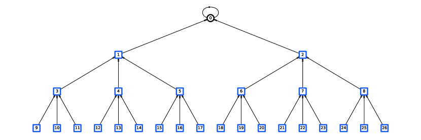
Figure 1. $3$-descending tree — Used code to generate this tree.

Note that in Fig. 1 that it is the same as a rhythmic tree with rhythm $(3).$ This is true for all integers.

Then, for rational $k$, it generates another rhythmic tree as described in [2]. The childcounts in Fig. 2 are periodic with pattern $2,1,\ldots$, meaning that it is a rhythmic tree with rhythm $(2,1).$

Figure 2. $\dfrac{3}{2}$-descending tree — Coded it to generate this tree.

Then, when $k$ is irrational, the behavior becomes slightly more chaotic. This specific example in Fig. 3 shows some particularly nice behavior due to our choice of $k=\phi$.

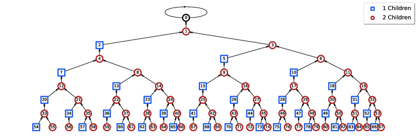
Figure 3. $\frac{1+\sqrt{5}}{2}\approx 1.618$-descending tree — Used a decimal approximation (up to 1000 digits) to generate this tree.

Note that this does not have a clearly obvious rhythm, with the childcounts not appearing to be periodic.

The remaining functions are defined based on a particular $k$-tree, so are technically also functions of $k$, but for brevity we will often not write the dependence on $k$ explicitly.

Definition 5.

For any $n\in\mathbb{N}$, let $\text{children}(n)=\{c\in\mathbb{N}:\lfloor\frac{c}{k}\rfloor=n\}$ be the set of children of $n$ in the $k$-tree. Then $h(n)=|\text{children}(n)|$ gives the child-count of $n$.

Remark 1.

For any $n\in\mathbb{N}_{+}$, $\min(\text{children}(n))=\lceil n\cdot k\rceil$.

Proof.

This follows immediately from the fact that $\lfloor\frac{\lceil nk\rceil}{k}\rfloor=n$, while $\lfloor\frac{\lceil nk\rceil-1}{k}\rfloor<n$. ∎

We can now formally prove the claim that the average child-count is $k$:

Remark 2.

$\lim_{N\to\infty}\frac{1}{N}\sum_{n=0}^{N-1}h(n)=k$.

Proof.

Notice that the sum $\sum_{n=0}^{N-1}h(n)$ counts every node from $0$ to the largest child of the node $N-1$. Thus,

$$\sum_{n=0}^{N-1}h(n)=1+\max(\text{children}(N-1))=\min(\text{children}(N))=\lceil N\cdot k\rceil,$$

from Remark 1. Then $\lim_{N\to\infty}\frac{1}{N}\lceil N\cdot k\rceil=k$. ∎

The child count $h(n)\in\{\lfloor k\rfloor,\lceil k\rceil\}$, and turns out to depend only on the quantity $\{n\cdot k\}$:

Definition 6.

For $n\in\mathbb{N}_{+}$, we call the fractional part $\{n\cdot k\}\in[0,1)$ the count indicator. The interval $(0,1-\{k\}]\subset[0,1)$ is called the floor-range and its complement $\{0\}\cup(1-\{k\},1)$ is called the ceil-range.

These definitions are motivated by the following foundational lemma:

Lemma 1.

For all $n\in\mathbb{N}$,

$$h(n)=\begin{cases}\lfloor k\rfloor&\emph{\text{if }}\{n\cdot k\}\in(0,1-\{k\}]\\ \lceil k\rceil&\emph{\text{otherwise}}.\end{cases}$$

Proof.

This statement is trivial if $k\in\mathbb{Z}$, so we assume now $k\notin\mathbb{Z}$ and $\lfloor k\rfloor+1=\lceil k\rceil$.

Notice that $\lfloor\frac{c}{k}\rfloor=n$ iff $c\in[nk,(n+1)k)$, thus $h(n)$ counts the integer points in this interval, whose width is $k=\lfloor k\rfloor+\{k\}$. Intuitively, the first part of the interval $[nk,nk+\lfloor k\rfloor)$ of width $\lfloor k\rfloor$ will always contain $\lfloor k\rfloor$ integer points. Then when $\{nk\}>1-\{k\}$, the remaining interval $[nk+\lfloor k\rfloor,nk+k)$ will “wrap around” one additional integer point. On the other hand, when $\{nk\}<1-\{k\}$, the fractional part strictly increases and does not wrap around an extra integer point.

In the boundary case $\{nk\}=0$, $nk\in\mathbb{Z}$, and the interval contains $\lceil k\rceil$ integer points $nk,nk+1,\ldots,nk+\lfloor k\rfloor$.

In the other boundary case $\{nk\}=1-\{k\}$, we have $nk+k\in\mathbb{Z}$, but the interval does not contain this rightmost boundary, and we thus have $\lfloor k\rfloor$ integer points $nk+k-1,nk+k-2,\ldots,nk+k-\lfloor k\rfloor$ in the interval. ∎

Notice that Lemma 1 implies that for rational $k\in\mathbb{Q}$, the child-count function $h(n)$ is periodic. See for example Fig. 2. Due to this periodicity we see that it is a rhythmic tree Definition 3.

Finally, we formally define the row-length sequence:

Definition 7.

$(r_{d})_{d=0}^{\infty}$ is the row-length sequence, where $r_{d}$ gives the number of nodes at depth $d$ in a $k$-tree. More formally, for a node $n\in\mathbb{N}$, the iterated function sequence $g_{0}=n$ and $g_{i+1}=\lfloor\frac{g_{i}}{k}\rfloor$ gives the path to the root. Then $\text{depth}(n)=\max(i:g_{i}=0)$ and $r_{d}=|\{n\in\mathbb{N}:\text{depth}(n)=d\}|$.

The sequence $r_{d}$ then intuitively grows at an exponential rate of $k$ as how $r_{d}\approx r_{d-1}\cdot k.$ However, due to the rounding off done by the floor function, it is not exactly this. So, we can define an asymptotics function on the row lengths.

Definition 8.

$\rho(k)=\lim_{d\to\infty}\frac{r_{d}}{k^{d}}$.

Note that we still need to show this limit exists.

3. Asymptotics of $r_{d}$

Theorem 1.

For any $k\in(1,\infty)\subset\mathbb{R}$, the constant $\rho(k)=\lim_{d\to\infty}\frac{r_{d}}{k^{d}}$ exists. Thus $r_{d}\sim\rho(k)\cdot k^{d}$.

Proof.

This is essentially a corollary of Proposition 1 from [3]. To be self-contained, we produce the proof in its entirety.

Observe that for any $n\in\mathbb{N}_{+}$, $\min(\text{children}(n))=\lceil n\cdot k\rceil$. We will then consider the sequence $f_{0}=1$ and $f_{i+1}=\lceil f_{i}\cdot k\rceil$. Notice that, subject to a change in indexing, this gives the leftmost elements in each row. For example, see

$f_{i}$	Value
$f_{0}$	1
$f_{1}$	2
$f_{2}$	4
$f_{3}$	7
$f_{4}$	12
$f_{5}$	20

Table 1. $f_{i}$ values for the $\phi$-tree, shown in Fig. 3.

We thus have $r_{d}=f_{d}-f_{d-1}$ for all $d>0$. Proposition 1 [3] shows there exists a constant $c(k)$ such that $f_{i}\sim c(k)\cdot k^{i}$. This will then imply

$$r_{d}\sim c(k)\cdot k^{d}-c(k)\cdot k^{d-1}=\frac{k-1}{k}c(k)\cdot k^{d},$$

thus we have $\rho(k)=\frac{k-1}{k}\cdot c(k)$.

To prove Proposition 1 from [3], or that $c(k)$ exists, we consider the sequence $(\frac{f_{i}}{k^{i}})_{i=0}^{\infty}$. First we show the sequence is nondecreasing, since

$$\frac{f_{i+1}}{k^{i+1}}=\frac{\lceil f_{i}\cdot k\rceil}{k^{i+1}}\geq\frac{f_{i}}{k^{i}}.$$

The sequence is also bounded above. We start with

$$\frac{f_{i+1}}{k^{i+1}}=\frac{\lceil f_{i}\cdot k\rceil}{k^{i+1}}<\frac{f_{i}\cdot k+1}{k^{i+1}}=\frac{f_{i}}{k^{i}}+\frac{1}{k^{i+1}},$$

and then with the base case $\frac{f_{0}}{k^{0}}=1$ we conclude

$$\frac{f_{n}}{k_{n}}<\sum_{i=0}^{n}\frac{1}{k^{i}}<\sum_{i=0}^{\infty}\frac{1}{k^{i}}=\frac{1}{1-1/k}=\frac{k}{k-1}.$$

Since the sequence $(\frac{f_{i}}{k^{i}})_{i=0}^{\infty}$ is nondecreasing and bounded from above, the limit $c(k)=\lim_{i\to\infty}(\frac{f_{i}}{k^{i}})$ exists. Moreover, we have the following bounds

$$1\leq c(k)\leq\frac{k}{k-1}.$$

This proves Proposition 1 from [3], in turn proving the existence of $\rho(k)$ for the asymptotics of $r_{d}$. ∎

Corollary 1.

$\frac{k-1}{k}\leq\rho(k)\leq 1$.

Proof.

The bounds on $c(k)$ as described in the proof of Theorem 1 alongside the relationship $\rho(k)=\frac{k-1}{k}\cdot c(k)$ gives the following bounds on $\rho$. ∎

So, we can now look at approximations of this data. The code for generating these approximations are attached in Appendix B. Some of the raw data is contained within Appendix C.

Within [3], Prop 3. they prove that there are jump discontinuities at the “Josephus points,” or rational numbers of the form $\frac{q}{q-1}$ where $q\in\mathbb{Z}_{+}.$ This is shown within Fig. 4. Since this is not relevant to the focus of the paper the proof of this will not be reproduced in its entirety.

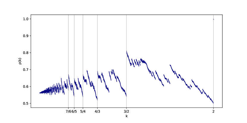
Figure 4. Jump Discontinuities from [3] — In Prop 3. from [3], there are jump discontinuities of an extremely nice form, where $c(a+\epsilon)=ac(a).$

Zooming out with Fig. 5, we can see what appears to be a more global pattern.

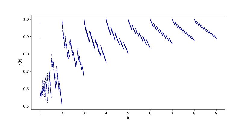
Figure 5. $\rho(k)$ for $1<k\leq 9$ — Approximated $\rho(k)$ for $10^{4}$ points.

One of these patterns appears to be periodic splits within the function. This is illustrated within Fig. 6. Within $n$ and $(n+1)$ for some integer $n\geq 1$, there are $(n+1)$ periodic ‘visible splits.’ Upon closer inspection, it appears there are also $(n+1)^{2}$ periodic ‘visible splits,’ with the best ones happening closest to $(n+1).$ This pattern visually holds, and the splits get smaller. Upon numerical testing, it is not clear if they share the same form as those described in [3].

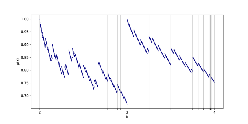
Figure 6. $\rho(k)$ for $1<k\leq 4$ with apparent splits — Approximated $\rho(k)$ for $10^{4}$ points, and also plotted the points of possible visible splits that seem to be self similar between $n$ and $n+1$.

4. $k$-Trees with Closed Form $\rho(k)$

Let us then define something that makes it more clear how to describe indicators.

Definition 9.

The child-count indicator graph for some $k>1$ is the set of functions $\{f_{i}|i=1,2,\ldots,\lceil k\rceil\}$, where $f_{i}(x)$ is defined to be the fractional part of the $i$th child of some $n$ where $x=\{nk\},$ so that $f_{i}:[0,1)\longrightarrow[0,1)$. If $\lceil k\rceil\neq\lfloor k\rfloor$, then we define $f_{\lceil k\rceil}:(1-\{k\},1]\longrightarrow[0,1)$ for the $ceil{k}$th child of a node $n$ if it exists.

Also, the ceil-range and floor-range are used to say $(1-\{k\},1]$ and $(0,1-\{k\}]$ respectively and are helpful to describe the child-count indicator graph in a more general sense.

What Definition 9 allows us to do is visualize the behavior of the “grand-children” of a node $n$. If we know it has fractional part $\{nk\},$ then we can see the fractional parts of its children, showing us its children’s children, leading to the terminology of “grandchildren.”

Lemma 2.

Let $k$ satisfy the equation $k=a+\frac{b}{k}$ for $a,b\in\mathbb{Z}$. Then for any node $n\in\mathbb{N}_{+}$, let $x=\{n\cdot k\}\in[0,1)$ be the count-indicator for $n$. Let $c_{1},\ldots,c_{h(n)}$ be the children of the node $n$. Then the $i$th smallest child $c_{i}$ has count-indicator

$$\{c_{i}\cdot k\}=\{(i-\{nk\})\cdot\frac{b}{k}\}.$$

Proof.

From Remark 1, we have $c_{1}=\lceil n\cdot k\rceil$, and more generally $c_{i}=\lceil n\cdot k\rceil+i-1$. We then have count indicator

$$\{c_{i}\cdot k\} =\{(\lceil n\cdot k\rceil+i-1)(a+\frac{b}{k})\}$$

$$=\{(\lceil n\cdot k\rceil+i-1)\cdot\frac{b}{k}\}$$

$$=\{(n\cdot k+1-\{n\cdot k\}+i-1)\cdot\frac{b}{k})\}$$

$$=\{(i-\{nk\})\cdot\frac{b}{k}\}.$$

∎

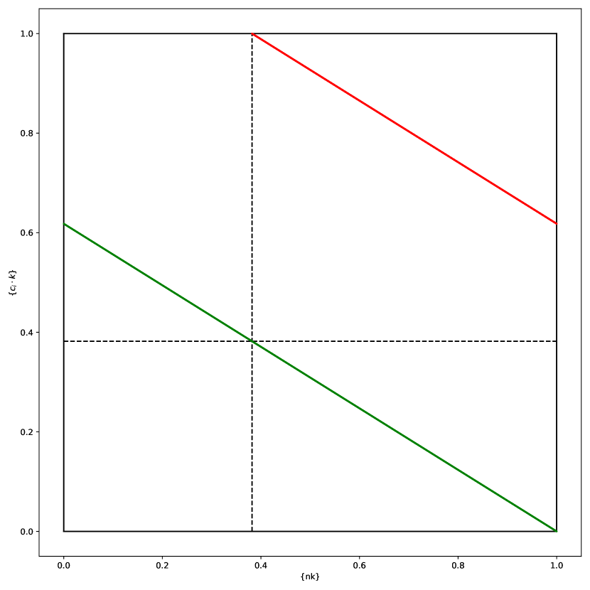
Figure 10. $\phi$ Grandparent Indicators

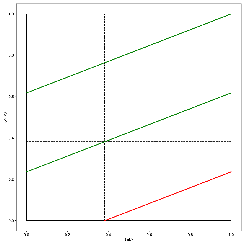
Figure 11. $a=3,b=-1$ Grandparent Indicators

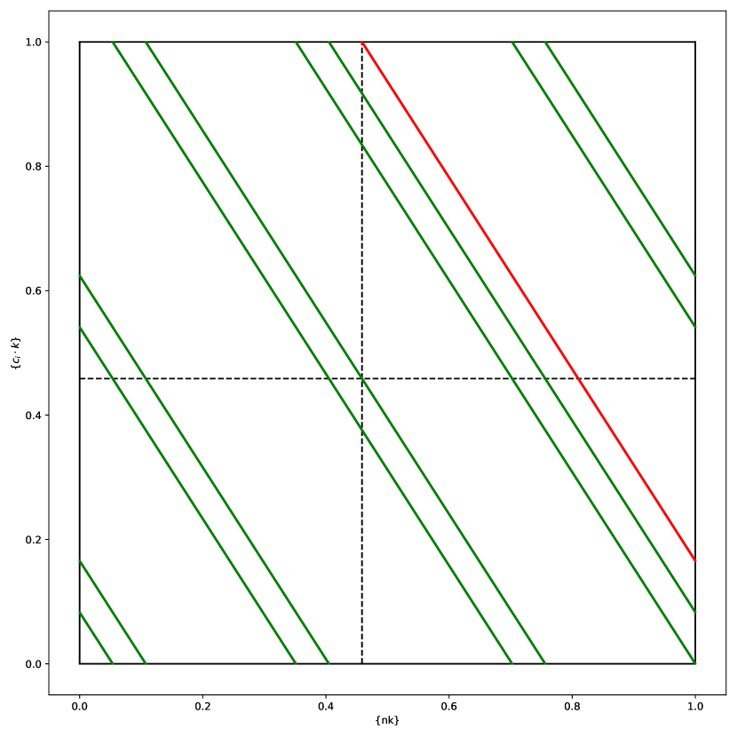
Figure 12. $a=3,b=7$ Grandparent Indicators

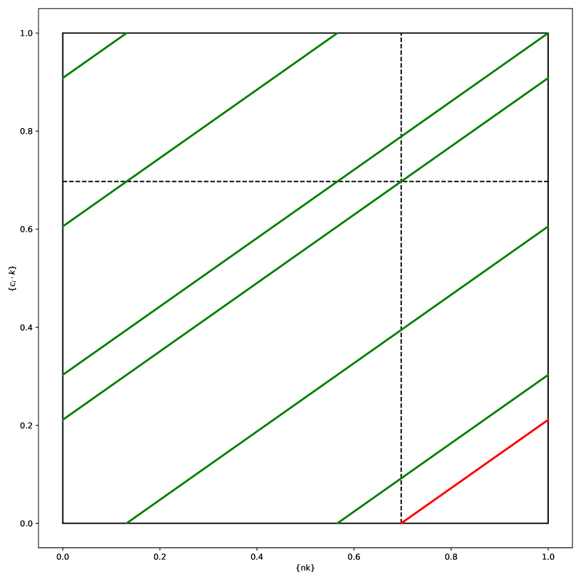
Figure 13. $a=5,b=-3$ Grandparent Indicators

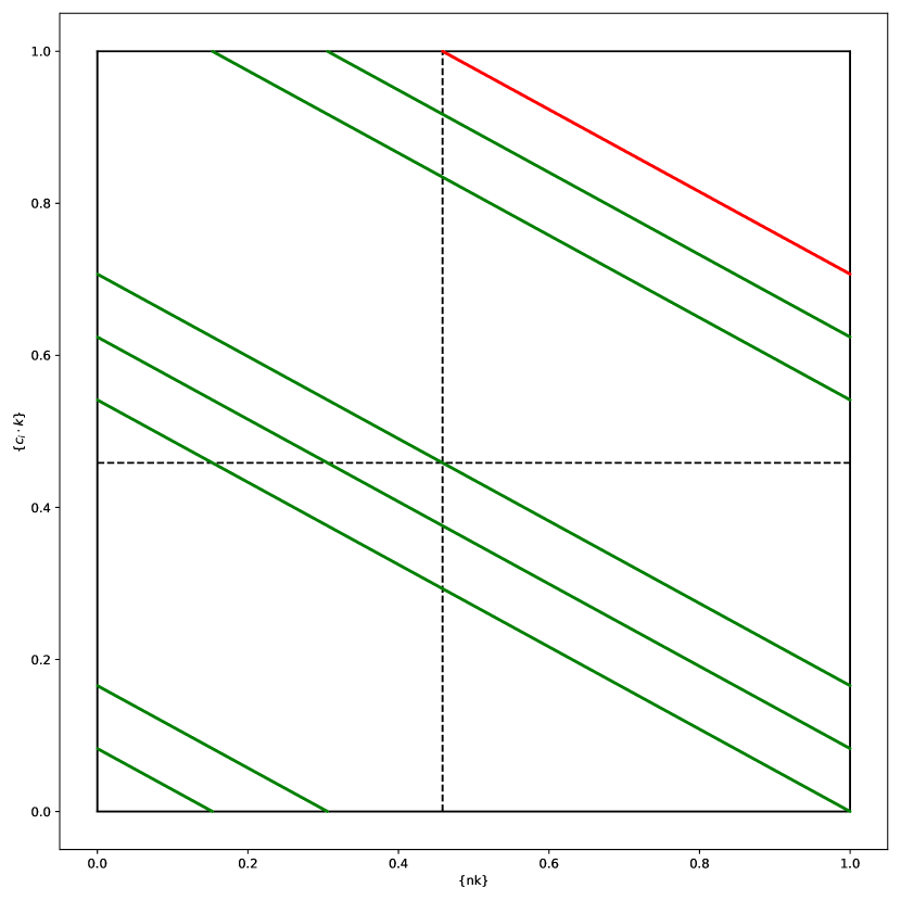
Figure 14. $a=5,b=3$ Grandparent Indicators

Some examples of Definition 9 and Lemma 2 are shown in Fig. 10, Fig. 11, Fig. 12, Fig. 13, Fig. 14, located in the Appendix D.

Theorem 2.

(Grandparent theorem) Let $a,b\in Z$ such that $a\geq 1$ and $1-a\leq b\leq a-1$. When $b\geq 0$, then there are always $b$ distinct lines in the ceil-range of the child count indicator graph for $k=\frac{a+\sqrt{a^{2}+4b}}{2}$. When $b$ is negative, then there are always $|b|$ distinct lines in the floor-range of the graph of $k$.

Proof.

Let $a,b\in Z$ such that $a\geq 1$ and $1-a\leq b\leq a-1$. Then, let $k=\frac{a+\sqrt{a^{2}+4b}}{2}$. Using Lemma 2,

$$\{c_{i+1}\cdot k\}-\{c_{i}\cdot k\} =\{(i+1-x)\cdot\frac{b}{k}\}-\{(i-x)\cdot\frac{b}{k}\}$$

$$=\{\frac{b}{k}\}$$

$$=\{k\},1-\{k\}(\text{depending on }b).$$

So, the difference between two consecutive childcount indicators is $\{k\}$ or $1-\{k\}$. The output ceil-range from Lemma 1 is of size $\{k\},$ and the floor-range is then $1-\{k\}.$ So, when one childcount indicator falls above or under that line, the next indicator “flips,” meaning that the amount of lines in the output ceil-range and floor-range stays constant throughout $x\in[0,1).$ So, this simplifies the proof in allowing us to choose for $x$ to show that there are specifically $b$ indicators in the specific output range.

The last step is now to find the number of solutions for $i$ in this expression, $1-\{k\}<\{\{k\}(i-x)\}<1,$ but now we can choose $x$. If $x=0,$ then the set of solutions is $\{\lfloor\frac{a}{b}\rfloor,\lfloor\frac{2a}{b}\rfloor,\lfloor\frac{3a}{b}\rfloor,\ldots,\lfloor\frac{(b-1)a}{b}\rfloor,\lfloor a\rfloor\}$, which contains $b$ solutions (in the nonnegative $b$ case). This is the set of solutions to $0<\{\{k\}(i-x)\}<1-\{k\}$ for the negative $b$ case. This then proves the theorem. ∎

Theorem 3.

Let $a,b\in\mathbb{Z}$ with $a\geq 1$ and $1-a<b<1+a$. For $k=\frac{a+\sqrt{a^{2}+4b}}{2}$, the row-length sequence for the $k$-tree satisfies the linear recurrence

$$r_{d}=a\cdot r_{d-1}+b\cdot r_{d-2},$$

with base case $r_{0}=1$, $r_{1}=\lceil k\rceil-1$.

Proof.

Let $a,b\in\mathbb{Z}$ with $a\geq 1$ and $1-a<b<1+a$. When $b\geq 0,$ we can see that $\lfloor k\rfloor=a.$ So, $r_{d}\geq ar_{d-1}$, as from Lemma 1 we know that each element from the previous row contributes at least $\lfloor k\rfloor$ children. With Theorem 2, we can see that each element in $r_{d-2}$ has $b$ children that have $\lceil k\rceil$ children, which creates the equality $r_{d}=ar_{d-1}+br_{d-2}.$ Instead, when $b<0,$ then $\lceil k\rceil=a,$ so $r_{d}\leq ar_{d-1}$. What happens then is $br_{d-2}$ actually takes away to compensate for the values with $\lfloor k\rfloor$ children. So,

$$r_{d}=ar_{d-1}+br_{d-2}.$$

∎

Corollary 2.

Let $a,b\in\mathbb{Z}$ with $a\geq 1$ and $1-a<b<1+a$. For $k=\frac{a+\sqrt{a^{2}+4b}}{2}$,

$$\rho(k)=\begin{cases}\dfrac{k}{\sqrt{a^{2}+4b}}&b>0\\[20.00003pt] \dfrac{k-1}{\sqrt{a^{2}+4b}}&b<0\\[20.00003pt] \dfrac{a-1}{a}&b=0\end{cases}$$

Proof.

Because of Theorem 3, we can find a closed formula for $r_{d}$.

As the theorem states, let $a,b\in\mathbb{Z}$ such that $a\geq 1,1-a<b<1+a$, and let $k_{1}=\frac{a+\sqrt{a^{4}+4b}}{2}$ and $k_{2}=\frac{a-\sqrt{a^{4}+4b}}{2}$.

Then, for the $k_{1}$ tree,

$$r_{d}=ar_{d-1}+br_{d-2}.$$

Like any recurrence problem, let $r_{d}=c^{d}$ for some constant $c$. Then,

$$c^{d} =ac^{d-1}+bc^{d-2}$$

$$c^{2} =ac+b$$

$$c^{2}-ac-b =0$$

$$c =k_{1},k_{2}.$$

So, we can plug in $c$ to $r_{d}$.

$$r_{d}=Ak_{1}^{d}+Bk_{2}^{d},$$

for some constants $A$ and $B$.

Now, we have to use the starting conditions $r_{0}=1,r_{1}=\lfloor k\rfloor$ to find $A$ and $B$. This is simply done by plugging in $d=0,1$. However, note that when $b\geq 0$, $\lfloor k\rfloor=a$, and when $b<0$, then $\lfloor k\rfloor=a-1.$

So, when $b\geq 0$, we can solve two linear systems.

$$\begin{bmatrix}1&1&1\\ k_{1}&k_{2}&a\end{bmatrix}\to\begin{bmatrix}1&0&\dfrac{a+\sqrt{a^{2}+4b}}{2\sqrt{a^{2}+4b}}=\dfrac{k_{1}}{\sqrt{a^{2}+4b}}\\[20.00003pt] 0&1&\dfrac{-a+\sqrt{a^{2}+4b}}{2\sqrt{a^{2}+4b}}=\dfrac{-k_{2}}{\sqrt{a^{2}+4b}}\end{bmatrix}$$

So, if $b\geq 0$,

$$r_{d}=\frac{k_{1}^{d+1}-k_{2}^{d+1}}{\sqrt{a^{2}+4b}}.$$

By solving the same original matrix with $a-1$ swapped with $a$, we can get that when $b<0$,

$$r_{d}=\frac{(k_{1}-1)^{d+1}-(k_{2}-1)^{d+1}}{\sqrt{a^{2}+4b}}.$$

Now, we can plug these closed formulas into $\rho(k)$. When $b\geq 0,$

$$\rho(k) =\lim_{d\to\infty}\dfrac{r_{d}}{k_{1}^{d}}$$

$$=\lim_{d\to\infty}\dfrac{k_{1}^{d+1}-k_{2}^{d+1}}{k_{1}^{d}\sqrt{a^{2}+4b}}$$

$$=\lim_{d\to\infty}\dfrac{k_{1}^{d+1}}{k_{1}^{d}\sqrt{a^{2}+4b}}$$

$$=\dfrac{k_{1}}{\sqrt{a^{2}+4b}}.$$

Similarly, when $b<0$,

$$\rho(k)=\dfrac{k_{1}-1}{\sqrt{a^{2}+4b}}.$$

Note that when $b=0$, then $k=a\in\mathbb{Z}$, so we can also write $\rho(k)=\dfrac{a-1}{a}$ due to $r_{d}=k^{d-1}(k-1).$ ∎

The values described in Corollary 2 are shown in Table 2.

Table 2. Values of the function $k=\frac{a+\sqrt{a^{2}+4b}}{2}$ for $a,b\in\mathbb{Z}$. Calculated the formula $k=\dfrac{a+\sqrt{a^{2}+4b}}{2}$ with decimal approximations for $-1\leq a\leq 7,$ and $-6\leq b\leq 8$.

So, by using Corollary 2, we can look at the closed formula for points that we do know on Fig. 7.

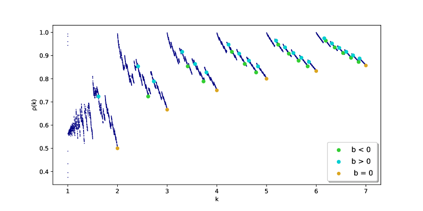
Figure 7. $\rho(k)$ for $1<k\leq 7$ with closed form — Approximated $\rho(k)$ for $10^{4}$ points, and also plotted the points that contain a closed formula.

5. Conclusion

So, we have found a closed formula for the irrational case, even when the rational case doesn’t have the same type of behavior. This is a rare case where irrationality seems to behave more nicely than their rational counterpart. Also, we have a closed formula for these golden-like trees. This is interesting and motivates the extension from a $k$-ary tree.

Now, for future work, there seems to be three different modes of progress. First would simply be to change from $\lfloor\frac{n}{k}\rfloor$ to $\lceil\frac{n}{k}\rceil$. This would be a $k$-ascending tree.

Definition 10.

For any $k\in(1,\infty)\subset\mathbb{R}$, the $k$-ascending tree is the rooted tree with nodes in $\mathbb{N}$, where every $n\in\mathbb{N}$ has the parent $\lceil\frac{n}{k}\rceil$.

Note that the root node of Definition 10 is not going to be $0$.

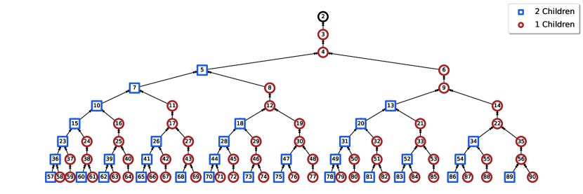
Figure 8. $\phi$-ascending tree — This generates a $\phi$-ascending tree. Modified the original code to use the ceiling function instead of floor

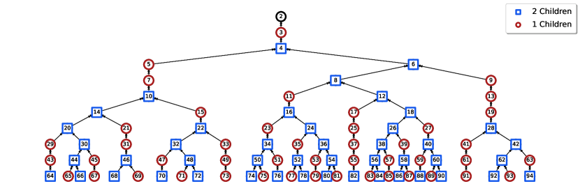
Figure 9. $\frac{3}{2}$-ascending tree — This generates a $\frac{3}{2}$-ascending tree. Note that this is still a rhythmic tree with a shift in indexing.

From observation, both examples seem to be shifted (as the root is not $0$), and Fig. 8 also seems to be flipped. From this it seems that a lot of the same ideas would carry over very nicely.

Second, it may be interesting to look at more complex $k$’s of the form $k=a+\frac{b}{k}+\frac{c}{k^{2}}.$ Instead of Theorem 3’s $r_{d}=a\cdot r_{d-1}+b\cdot r_{d-2}$, we may have the recurrence $r_{d}=a\cdot r_{d-1}+b\cdot r_{d-2}+c\cdot r_{d-3}.$ It would be nice if this was true, but it doesn’t seem like it would work due to Theorem 3’s reliance on the grandparent indicator only going back to $r_{d-2}$.

Also, note that the $\phi$-tree has a regular language that describes its paths. In [2], they say that all rational numbers $k$ that are not integers do not have this property in the $k$-tree, so it would be interesting to see which other irrational numbers have this property. This isn’t true for other “golden-like” numbers, or numbers of the form $k=a+\frac{b}{k}.$

Furthermore, one of the original reasons that [2] researched rhythms was their connection to fractional bases. When $k$ is a rational number, the language describing paths in the $k$-tree form a bijection with the natural numbers in base $k$. In the irrational $k$ case, the path to a node $n$ in the $k$-tree could be seen as some sort of base-$k$ representation of $n$, but addition is not as clear anymore.

Within this paper there was the surprising connection to the Josephus problem [3], and the article [1] looks specifically at the constant $\rho(\frac{3}{2})$ in regard to the Collatz Conjecture and mentions the Josephus problem. The connection to the Collatz Conjecture is light, as one can simplify the process into this tree. The Collatz Conjecture states that if you take some $n\in\mathbb{N}$, if it is even divide it by 2, otherwise take $3n+1$ and continue this process, you will always reach 1. The article talks about the simplification of this process to just $\lfloor\frac{3n}{2}\rfloor$ to remove the complexity and arrives at the $c(\frac{3}{2})$ constant to describe the tree that this process generates, which is the same as our $k$-descending tree.

These connections to the Josephus Problem and others can be further fleshed out if one found a more direction connection by figuring out how to represent the Josephus problem with trees. One idea could be that the indices of the vertices represent the players in the Josephus problem.

This research was presented at the Sofia, Bulgaria WFNMC conference in the summer of 2022. The authors would like to thank the administration there.

Agniv Sarkar Eric Severson

Appendix A Tree Generation Code

This is the code used to generate the $k$-tree figures.

⬇

1from decimal import *

2from re import X

3import networkx as nx

4import matplotlib.pyplot as plt

5from math import floor, ceil

6import os

7import random

8

9save_as = 4

10save_location = "./drive/MyDrive/Figures"

11largest_can_draw = 1000

12

13os.makedirs(save_location, exist_ok=True)

14

15def rows(n, k):

16 """ returns r0...r_n in the k-tree """

17 r = row_gen(Decimal(k))

18 return [next(r) for x in range(n)]

19

20def left_gen(k):

21 """ generator for leftmost nodes in the k-tree """

22 yield 0

23 l = 1

24 while True:

25 yield l

26 l = ceil(Decimal(l) * Decimal(k))

27

28def row_gen(k):

29 """ generator for row lengths in the k-tree"""

30 left_iter = left_gen(k)

31 last_left = next(left_iter)

32 while True:

33 next_left = next(left_iter)

34 yield next_left - last_left

35 last_left = next_left

36

37def fancytree(largest, k, save = True):

38 """

39 Draws a k-tree up to largest value given.

40 To use depth instead, pass on the max_n from here:

41

42 depth = 10 # some number of rows

43 max_n = 0

44 row_lengths = rows(depth, k)

45 for row in row_lengths:

46 max_n += row

47

48 """

49 G = nx.DiGraph()

50 fl = []

51 ce = []

52

53 # CONNECTING THE NODES

54 for x in range(1, largest):

55 G.add_edge(floor(x/k), x)

56 if Decimal(k*x) - floor(Decimal(k*x)) < 1 - k + floor(k):

57 fl.append(x)

58 else:

59 ce.append(x)

60

61 # DRAWING THE TREE

62 if (largest > largest_can_draw):

63 return

64 plt.clf()

65 pos = hierarchy_pos(nx.Graph(G), 0)

66 G.add_edge(0, 0)

67

68 # DRAWS THE NODES WITH COLOR

69 nsize = 450

70 lwidth = 3.5

71 nx.draw(G.reverse(), pos, nodelist = [0], node_size = nsize, node_color = ’#ffffff’, node_shape = "o", edgecolors=’#000000’, linewidths = lwidth, with_labels = True)

72 nx.draw(G.reverse(), pos, label = str(floor(k)) + " Children", nodelist = fl, node_size = nsize, node_color = ’#ffffff’, node_shape = "s", edgecolors=’#1357eb’, linewidths = lwidth, with_labels = True)

73 nx.draw(G.reverse(), pos, label = str(ceil(k)) + " Children", nodelist = ce, node_size = nsize, node_color = ’#ffffff’, node_shape = "o", edgecolors=’#ab1a1a’, linewidths = lwidth, with_labels = True)

74 if abs(k - int(k)) <= 10**(-5):

75 pass

76 else:

77 plt.legend(loc = ’best’, fontsize = ’xx-large’, markerscale = .45,

78 labelspacing = .7,

79 title_fontsize = ’xx-large’, borderpad = .6, shadow = True)

80 if save:

81 plt.savefig(save_location+str(round(k, save_as))+"tree.pdf", format = ’pdf’, dpi=300)

82 plt.show()

83

84def hierarchy_pos(G, root=None, width=1., vert_gap = 0.2, vert_loc = 0, leaf_vs_root_factor = 0.5):

85 """

86 Source: https://github.com/ryoji-kubo/CurvatureAnalysis/blob/main/utils.py

87 Source: https://github.com/BaseMax/BinaryTreeDiagramDrawing/blob/master/tree.py

88 """

89

90 if root is None:

91 if isinstance(G, nx.DiGraph):

92 root = next(iter(nx.topological_sort(G))) #allows back compatibility with nx version 1.11

93 else:

94 root = random.choice(list(G.nodes))

95

96 if not nx.is_tree(G):

97 raise TypeError(’cannot use hierarchy_pos on a graph that is not a tree’)

98

99 def _hierarchy_pos(G, root, leftmost, width, leafdx = 0.2, vert_gap = 0.2, vert_loc = 0,

100 xcenter = 0.5, rootpos = None,

101 leafpos = None, parent = None):

102

103 if rootpos is None:

104 rootpos = {root:(xcenter,vert_loc)}

105 else:

106 rootpos[root] = (xcenter, vert_loc)

107 if leafpos is None:

108 leafpos = {}

109 children = list(G.neighbors(root))

110 leaf_count = 0

111 if not isinstance(G, nx.DiGraph) and parent is not None:

112 children.remove(parent)

113 if len(children)!=0:

114 rootdx = width/len(children)

115 nextx = xcenter - width/2 - rootdx/2

116 for child in children:

117 nextx += rootdx

118 rootpos, leafpos, newleaves = _hierarchy_pos(G,child, leftmost+leaf_count*leafdx,

119 width=rootdx, leafdx=leafdx,

120 vert_gap = vert_gap, vert_loc = vert_loc-vert_gap,

121 xcenter=nextx, rootpos=rootpos, leafpos=leafpos, parent = root)

122 leaf_count += newleaves

123

124 leftmostchild = min((x for x,y in [leafpos[child] for child in children]))

125 rightmostchild = max((x for x,y in [leafpos[child] for child in children]))

126 leafpos[root] = ((leftmostchild+rightmostchild)/2, vert_loc)

127 else:

128 leaf_count = 1

129 leafpos[root] = (leftmost, vert_loc)

130 return rootpos, leafpos, leaf_count

131

132 xcenter = width/2.

133 if isinstance(G, nx.DiGraph):

134 leafcount = len([node for node in nx.descendants(G, root) if G.out_degree(node)==0])

135 elif isinstance(G, nx.Graph):

136 leafcount = len([node for node in nx.node_connected_component(G, root) if G.degree(node)==1 and node != root])

137 rootpos, leafpos, leaf_count = _hierarchy_pos(G, root, 0, width,

138 leafdx=width*1./leafcount,

139 vert_gap=vert_gap,

140 vert_loc = vert_loc,

141 xcenter = xcenter)

142 pos = {}

143 for node in rootpos:

144 pos[node] = (leaf_vs_root_factor*leafpos[node][0] + (1-leaf_vs_root_factor)*rootpos[node][0], leafpos[node][1])

145 xmax = max(x for x,y in pos.values())

146 for node in pos:

147 pos[node]= (pos[node][0]*width/xmax, pos[node][1])

148 return pos

Listing 1: Tree Generation Code

Appendix B $\rho$ Code

This is the code used to generate $\rho(k)$ values.

⬇

1import pandas as pd

2import numpy as np

3from math import floor, ceil, sqrt, log

4from decimal import *

5import matplotlib.pyplot as plt

6

7source = "./drive/MyDrive/Figures/rho.csv"

8

9def resetRho():

10 """ Empties out if error is encountered """

11 df = pd.DataFrame({’val’:[],’out’:[],’precision’:[]})

12 df.to_csv(source, index=False)

13 return df

14

15def getPrec(k, df):

16 """ Returns the stored precision for rho(k) in the csv. 0 if not found """

17 try:

18 return df.loc[min(df.loc[df.val == k].index)].precision

19 except:

20 return 0

21

22def addRho(df, info):

23 """ Adds value to the stored csv. """

24 inside = getPrec(info[0], df) != 0

25 if inside:

26 df.loc[(df["val"] == info[0])] = info

27 else:

28 df.loc[len(df)] = info

29 return df

30

31def writeRho(df):

32 """ Writes to an external csv for storage """

33 df.to_csv(source, index = False)

34

35def left_gen(k):

36 """ Generator for leftmost nodes """

37 yield 0

38 l = 1

39 while True:

40 yield l

41 l = ceil(Decimal(l) * Decimal(k))

42

43def row_gen(k):

44 """ Generator for row lengths """

45 left_iter = left_gen(k)

46 last_left = next(left_iter)

47 while True:

48 next_left = next(left_iter)

49 yield next_left - last_left

50 last_left = next_left

51

52def get_rho(k, min_row_size = 10**3, eps = 10 ** -3, iter_upper_bound = 10 ** 2):

53 """

54 If a rho(k) value is not found within rho.csv, generate it.

55 Also runs if a higher precision value

56 precision is defined with:

57 minimum row size to start at, upper bound to stop at, eps, decimal precision

58 """

59 if k <= 1:

60 return None

61 elif abs(k - int(k)) < 10**(-1000000):

62 return Decimal((k-1))/Decimal(k)

63 row = row_gen(k)

64 last_c = 1

65 r = next(row)

66 c = 1

67 while r < min_row_size:

68 r = next(row)

69 c += 1

70 for i in range(c, iter_upper_bound+c):

71 next_c = Decimal(next(row)) / Decimal(k) ** Decimal(i)

72 if abs(next_c - last_c) < eps:

73 return (next_c + last_c) / 2

74 last_c = next_c

75 return next_c

76

77def find_rho(k, min_row_size = 10**3, eps = 10 ** -3, iter_upper_bound = 10 ** 2):

78 """

79 Gets the value of rho(k) to some precision, either through rho.csv or generating it.

80 """

81 try:

82 df = pd.read_csv(source)

83 except FileNotFoundError:

84 return get_rho(k, min_row_size=min_row_size, eps=eps, iter_upper_bound=iter_upper_bound)

85 except:

86 df = resetRho()

87 if abs(k - int(k)) < 10**(-100):

88 prec = np.inf

89 else:

90 prec = log(min_row_size*eps**(-1)*iter_upper_bound*getcontext().prec, 10)

91 curPrec = getPrec(k, df)

92 if curPrec < prec or curPrec == 0:

93 rho = get_rho(k, min_row_size=min_row_size, eps=eps, iter_upper_bound=iter_upper_bound)

94 writeRho(addRho(df, [k, rho, prec]))

95 return rho

96 elif curPrec >= prec:

97 return df.loc[min(df.loc[df.val == k].index)].out

98

99x = np.linspace(1 + 10**(-6), 6, 10**5)

100plt.scatter(x, np.array(list(map(find_rho, x))), s = 0.1)

101plt.xlabel(’k’)

102plt.ylabel(’ρ(k)’)

103plt.title(f’Estimated values of ρ(k) for 100000 random values 1 < k < 6’)

104plt.show()

Listing 2: $\rho(k)$ Approx. Code

Appendix C $\rho$ Raw Data

This is some recorded raw data generated by the code. Note that there appears to be some rounding off that happens as the data is written to the csv file. The data is actually too large to be typically viewed with tools like csvsimple. The link is at https://github.com/agniv-the-marker/rho-stuff.

Appendix D Grandparent Indicator Figures

References

- [1] James Grime, Kevin Knudson, Pamela Pierce, Ellen Veomett, and Glen Whitney. Beyond pi and e: a collection of constants. Math Horizons, 29(1):8–12, 2022.
- [2] Victor Marsault and Jacques Sakarovitch. Rhythmic generation of infinite trees and languages. arXiv preprint arXiv:1403.5190, 2014.
- [3] Andrew M Odlyzko and Herbert S Wilf. Functional iteration and the josephus problem. Glasgow Mathematical Journal, 33(2):235–240, 1991.