Shortcuts to Adiabaticity in Krylov Space

Abstract

Shortcuts to adiabaticity provide fast protocols for quantum state preparation in which the use of auxiliary counterdiabatic controls circumvents the requirement of slow driving in adiabatic strategies. While their development is well established in simple systems, their engineering and implementation are challenging in many-body quantum systems with many degrees of freedom. We show that the equation for the counterdiabatic term, equivalently the adiabatic gauge potential, is solved by introducing a Krylov basis. The Krylov basis spans the minimal operator subspace in which the dynamics unfolds and provides an efficient way to construct the counterdiabatic term. We apply our strategy to paradigmatic single and many-particle models. The properties of the counterdiabatic term are reflected in the Lanczos coefficients obtained in the course of the construction of the Krylov basis by an algorithmic method. We examine how the expansion in the Krylov basis incorporates many-body interactions in the counterdiabatic term.

I Introduction

In noisy quantum devices, dominant in the NISQ era [1], the prospects of implementing exact adiabatic control protocols are dim. Noise generally lowers the fidelity of preparing a target quantum state, making the dynamics not unitary, and leading to a final mixed state. The presence of noise further limits the admissible operation time in adiabatic protocols, e.g., in adiabatic quantum computing and quantum annealing. In these devices, noise can act as a heating source leading to excitation formation [2, 3], precluding the goal of finding the low-energy configuration of a given problem Hamiltonian.

The ubiquitous presence of noise in current NISQ devices forces us to rethink the use of adiabatic strategies. A natural approach is operating in time scales where environmental noise is negligible. A demonstration of this approach has recently been reported in quantum annealing devices, where noise-induced errors generated for moderate operation times [4] can be eliminated by shortening the duration of the process [5]. However, this strategy generally limits the efficiency of the computation as a result of the adiabatic theorem, whether one considers the system closed [6] or open [7]. An alternative approach relies on optimally tailoring the time-dependence of the parameters that are varied in time in the system of interest (e.g., the harmonic frequency in a trapped system or a magnetic field in a spin system) [8]. This is the principle behind the so-called boundary cancellation method that reduces excitations by devising smooth protocols in view of the adiabatic theorem in either isolated or open systems [9, 10, 7]. Such an approach requires no additional control fields, easing the implementation of the driving protocols in the laboratory [11], but provides limited advantages in the speedup, and technical assumptions in the adiabatic theorem may restrict its applicability.

Shortcuts to Adiabaticty (STAs) provide an alternative approach [12, 13, 14, 15]. They enforce the nonadiabatic following of a prescribed adiabatic trajectory of interest, tailoring nonadiabatic excitations utilizing auxiliary control fields. In other words, STAs remove the requirement for slow driving in adiabatic protocols, leading to the preparation of the same target state in a shorter time. By now, several experiments have demonstrated the use of STAs in ultracold atoms [16, 17, 18, 19, 20, 21, 22, 23], nitrogen-vacancy centers [24, 25], trapped ions [26], and superconducting qubits [27], among others.

While various techniques have been developed to engineer STAs, counter-diabatic (CD) driving stands out among them by providing a universal approach for any system in isolation. The early formulation due to Demirplak and Rice [28, 29, 30], independently developed by Berry [31], assumes the dynamics to be unitary and the system Hamiltonian to be diagonalizable at all times. However, progress over the last decade has shown that STAs can be applied to open quantum systems [32, 33, 34, 35, 36], as demonstrated in a pioneering experiment [37].

From the outset, the need for the system Hamiltonian to be diagonalizable at all times precludes the application of CD driving in important scenarios where such knowledge is unavailable, e.g., in quantum annealing. However, the development of approximate methods to engineer CD controls has challenged and de facto removed this requirement. Specifically, the early proposal of using digital methods for quantum simulation to realize CD controls [38], in combination with variational methods [39, 40, 41], has led to a framework for digitized-CD quantum driving for quantum algorithms [42, 43], that include the use of STA in adiabatic quantum computation [44] and quantum optimization [45, 46, 47].

The nature of the CD controls remains currently an issue. In a system with many degrees of freedom, finding an efficient prescription to determine the CD fields is generally challenging. The first works exploring STA by CD driving in many-body quantum systems showed that the CD controls generally involved many-body interactions of arbitrary rank (one-body, two-body, etc.) [38, 48, 49]. In addition, CD terms are generally spatially nonlocal [49]. In systems of continuous variables, such as a harmonic oscillator or ultracold gases, CD terms cannot always be realized by applying an external potential [12, 50] but may involve nonconservative momentum-dependent Hamiltonian terms [51, 52, 53]. Likewise, in spin systems, CD terms may involve interactions among distant spins [38, 48, 49]. As a result, one of the pressing problems in the development of STA is to find systematic approaches to tailor CD terms. One option is to find unitarily equivalent Hamiltonians for which STAs can be implemented exactly with experimentally available resources [54, 52, 53]. Another relies on approximate protocols, determined through variational methods [49, 39, 40, 55, 56] or otherwise [48, 57, 58].

Current general approaches to engineering STA by CD driving are blind to any structure or symmetry in the actual dynamics. However, it is known that the presence of dynamical symmetries in a given process can significantly simplify the CD protocols required to control it and render the implementation of STA experimentally realizable. In cases where a dynamical symmetry is known, one can identify the CD controls in terms of the elements of a closed Lie algebra [59]. However, the application of this approach has been limited to the restricted set of examples in which dynamical symmetries are known, i.e., few-level systems [60] and scale-invariant processes [61].

Further progress calls for novel approaches that systematically unravel and exploit any structure in the dynamics of the process to be controlled. This work introduces an approach that achieves this goal by formulating CD driving in Krylov space. Krylov subspace methods have a long tradition in numerical recipes and can be efficiently implemented using the Lanczos algorithm and its variants [62]. In time-dependent quantum mechanics, Krylov space describes the minimal subspace in which the dynamics unfolds, greatly easing the computational resources to describe time-evolution [63]. They are further useful in foundations of quantum physics to characterize operator growth [64, 65, 66, 67] and the fundamental speed limits governing it [68, 69]. Consider the case of the quantum dynamics in the Heisenberg representation. Given an observable of interest $O_{0}$ and a generator of evolution $H$, the evolution of the observable is set by $O(t)=U^{\dagger}(t)O_{0}U(t)$ where $U(t)$ is the time-evolution operator. For time-independent Hamiltonians such evolution admits the expansion $O(t)=\sum_{n=0}^{\infty}(it)^{n}\mathcal{L}^{n}O_{0}/n!$ with the Liouvillian $\mathcal{L}(\cdot)=[H,\cdot]$. The dynamics generates the set of operators $\{\mathcal{L}^{n}O_{0}\}_{n=0}^{\infty}$ that are not orthonormal and generally live in an operator subspace known as the Krylov space. The Lanczos algorithm can be used to construct a basis in Krylov space and further provides the Lanczos coefficients that determine the entries of the matrix representation of the Liouvillian in the Krylov basis.

In this work, we introduce a formulation of CD driving in Krylov space using the celebrated Lanczos algorithm. In doing so, we exploit the minimal operator subspace to identify the CD term required to control the dynamics. We circumvent the need for approximate and variational methods in the state-of-the-art engineering of STA, by providing an exact close-form expression for the CD term in the Krylov basis and the Lanczos coefficients. We illustrate this approach in various canonical examples, including two- and three-level systems, the harmonic oscillator. We also demonstrate our results with integrable, nonintegrable, and disordered quantum spin chains.

II Adiabatic gauge potential and counterdiabatic driving

We treat closed quantum systems with the Hamiltonian operator $H(\lambda)$ parametrized by a set of parameters $\lambda=(\lambda_{1},\lambda_{2},\dots)$. Throughout this paper, we denote an operator or a matrix with a capital letter. We consider the relations

$$H(\lambda)|n(\lambda)\rangle=\epsilon_{n}(\lambda)|n(\lambda)\rangle,$$ (1)

$$A(\lambda)|n(\lambda)\rangle=i\partial_{\lambda}|n(\lambda)\rangle.$$ (2)

$|n(\lambda)\rangle$ represents an eigenstate of the Hamiltonian with the eigenstate $\epsilon_{n}(\lambda)$. The phase of the eigenstate is fixed by requiring the relation $\langle n(\lambda)|\partial_{\lambda}n(\lambda)\rangle=0$. Then, the adiabatic gauge potential (AGP) operator $A=(A_{1},A_{2},\dots)$ is introduced by differentiating the eigenstate with respect to $\lambda$. We note that $A$ is common to all possible eigenstates.

One of the prominent applications of the AGP is the CD driving [28, 29, 30, 31, 70]. For time-varying parameters $\lambda(t)$, we consider the time evolution

$$i\partial_{t}|\psi(t)\rangle=\{H[\lambda(t)]+H_{\rm CD}(t)\}|\psi(t)\rangle.$$ (3)

Here, the CD term is introduced as $H_{\rm CD}(t)=\dot{\lambda}(t)\cdot A[\lambda(t)]$ where the overdot denotes the time derivative. It prevents the nonadiabatic transitions with respect to $H$, which means that the solution of the Schrödinger equation (3) is exactly given by the adiabatic state of $H$:

$$|\psi(t)\rangle=\sum_{n}e^{-i\int_{0}^{t}ds\,\epsilon_{n}[\lambda(s)]}|n[\lambda(t)]\rangle\langle n[\lambda(0)]|\psi(0)\rangle.$$ (4)

Even when the implementation of the CD term is challenging, we can use the CD term to assess the nonadiabatic effects [71].

It is a nontrivial problem to obtain the explicit form of the AGP for a given Hamiltonian, though the spectral representation is easily obtained as

$$\langle m(\lambda)|A(\lambda)|n(\lambda)\rangle=i\frac{\langle m(\lambda)|\partial_{\lambda}H(\lambda)|n(\lambda)\rangle}{\epsilon_{n}(\lambda)-\epsilon_{m}(\lambda)}(1-\delta_{m,n}).$$ (5)

The main aim of the present work is to find a systematic way to obtain the operator form of the AGP. The AGP satisfies

$$\mathcal{L}_{\lambda}\left[\partial_{\lambda}H(\lambda)-i\mathcal{L}_{\lambda}A(\lambda)\right]=0.$$ (6)

This relation was used to find an approximate AGP by variational methods [39, 40, 72]. We exploit this relation to obtain the exact form of the AGP.

As an alternative useful relation, we can use the integral representation [40, 73]

$$A(\lambda) = -\frac{1}{2}\lim_{\eta\to 0}\int_{-\infty}^{\infty}ds\,{\rm sgn}\,(s)e^{-\eta|s|}$$ (7)

$$\times e^{iH(\lambda)s}\partial_{\lambda}H(\lambda)e^{-iH(\lambda)s}.$$

This relation motivates us to examine the expansion

$$A(\lambda)=i\sum_{k}\alpha_{k}^{\rm nc}(\lambda)\mathcal{L}_{\lambda}^{2k-1}\partial_{\lambda}H(\lambda),$$ (8)

which denotes that the operators in the AGP are generated from the nested commutators $\mathcal{L}^{2k-1}\partial H$ at odd orders. We note that the variable $s$ in the integral representation represents a fictitious time. The unitary $e^{-iH(\lambda)s}$ is interpreted as the time evolution operator in the fictitious time with no need for the time-ordered product, as $H(\lambda)$ is independent of $s$. When we keep all possible operators generated from the nested commutators, the exact AGP can be obtained by solving the equation for $\alpha_{k}^{\rm nc}$ from Eq. (6). Practically, we consider a truncation of the operator series to obtain an approximate AGP. The infinite series by nested commutators produces the same type of operators many times and it is not clear how many terms we should keep to obtain a required accuracy. To treat the AGP systematically, we rearrange the expansion in Eq. (8) and represent the AGP in a finite series by using a set of orthonormal Krylov basis elements.

III Krylov expansion

III.1 Inner product, basis operators, and vector representation of operators

In the Krylov method [63], we use a set of operators satisfying an orthonormal relation. To define the orthonormality of operators, we first introduce the inner product for an arbitrary pair of operators $X$ and $Y$ as

$$(X,Y)=\frac{1}{2}{\rm Tr}[\rho(H)(X^{\dagger}Y+YX^{\dagger})].$$ (9)

The operators are not necessarily Hermitian. $\rho(H)$ represents a positive-definite Hermitian operator , which is not necessarily normalized. We note that the present method is applicable even when the Hilbert space dimension is infinite and the energy spectrum is continuous, provided that $\rho(H)$ is chosen appropriately. We see in the following that the result of the AGP is independent of the choice of $\rho(H)$. What is important is that $\rho(H)$ commutes with $H$. We have

$$(X,\mathcal{L}X)=0,$$ (10)

$$(X,\mathcal{L}Y)^{*}=(Y,\mathcal{L}X),$$ (11)

for Hermitian operators $X$ and $Y$.

To find an explicit representation of the superoperator $\mathcal{L}$, we introduce a set of basis operators $X=(X_{1},X_{2},\dots)$, that are Hermitian and orthonormal with each other:

$$(X_{\mu},X_{\nu})=\delta_{\mu,\nu}.$$ (12)

The number of operators is not specified here and is discussed in the following after clarifying the aim of the analysis. Generally, for a given quantum system, it is equal to or smaller than the square of the dimension of the Hilbert space.

One of the aims of introducing the basis operators is that the superoperator $\mathcal{L}$ can be represented by an antisymmetric Hermitian matrix $L$. It has elements

$$L_{\mu\nu}=(X_{\mu},\mathcal{L}X_{\nu}),$$ (13)

and satisfies $L^{\dagger}=L$ and $L^{\rm T}=-L$. The diagonal components are equal to zero and each of the off-diagonal components is purely imaginary. Corresponding to the matrix representation of superoperator, a vector represents an operator. We write the Hamiltonian

$$H=h\cdot X \Leftrightarrow |H\rangle=(h_{1},h_{2},\dots)^{\rm T},$$ (14)

and the AGP

$$A=a\cdot X \Leftrightarrow |A\rangle=(a_{1},a_{2},\dots)^{\rm T}.$$ (15)

Then, we obtain a vector representation of Eq. (6) as

$$L\left(|\partial_{\lambda}H\rangle-iL|A\rangle\right)=0.$$ (16)

It is not a difficult problem to obtain the formal solution of this equation by using the spectral representation of $L$. However, $L$ is generally a matrix of large size and the diagonalization is much more difficult than that of the Hamiltonian $H$. We resolve this problem in the following by introducing an algorithmic method.

III.2 Lanczos algorithm and Krylov basis

Equation (16) implies that the AGP $|A\rangle$ is constructed from a linear combination of $L^{n}|\partial H\rangle$ with $n=1,2,\dots$. We prepare the normalized vector $|\theta_{0}\rangle$ from the relation

$$b_{0}|\theta_{0}\rangle=|\partial H\rangle.$$ (17)

The coefficient $b_{0}$ represents the normalization factor and is written as

$$b_{0}^{2}=\langle\partial H|\partial H\rangle=(\partial H,\partial H).$$ (18)

We note that the normalized vector and the coefficient are defined for each component of $\lambda$. The same applies to the quantities introduced in the following. We abbreviate the component index to simplify the notation. Then, the new normalized basis $|\theta_{1}\rangle$ is defined from

$$b_{1}|\theta_{1}\rangle=L|\theta_{0}\rangle.$$ (19)

$|\theta_{1}\rangle$ is orthogonal to $|\theta_{0}\rangle$. We repeat the same procedure by using the relation

$$b_{n}|\theta_{n}\rangle=L|\theta_{n-1}\rangle-b_{n-1}|\theta_{n-2}\rangle,$$ (20)

with $n=2,3,\dots$. The positive coefficient $b_{n}$ is chosen so that $|\theta_{n}\rangle$ is normalized. By construction, the introduced vectors satisfy the orthonormal relation $\langle\theta_{m}|\theta_{n}\rangle=\delta_{m,n}$. When the dimension of the Hilbert space is finite, the number of basis elements must be finite, which means that there exists an integer $d$ satisfying $L|\theta_{d-1}\rangle-b_{d-1}|\theta_{d-2}\rangle=0$. The number of the basis vectors is given by $d$ which we refer to as the Krylov dimension.

This way of constructing a basis set is nothing but the Lanczos algorithm since the matrix $L$ is brought to a tridiagonal form as $L=VTV^{\dagger}$, where $V=(|\theta_{0}\rangle\ |\theta_{1}\rangle\ \cdots\ |\theta_{d-1}\rangle)$ and

$$T=\left(\begin{array}[]{cccccc}0&b_{1}&0&&&\\ b_{1}&0&b_{2}&&&\\ 0&b_{2}&0&&&\\ &&&\ddots&&\\ &&&&0&b_{d-1}\\ &&&&b_{d-1}&0\end{array}\right).$$ (27)

We can also write

$$L=\sum_{n=1}^{d-1}b_{n}\left(|\theta_{n}\rangle\langle\theta_{n-1}|+|\theta_{n-1}\rangle\langle\theta_{n}|\right).$$ (28)

Generally, for a given matrix $L$ and an initial basis element $|\theta_{0}\rangle$, we can render the matrix in tridiagonal form algorithmically. We find in the following that the present choice of the initial basis in Eq. (17) is convenient to solve Eq. (16).

The introduction of the orthonormal basis vectors corresponds to that of the orthonormal basis operators $|O_{n}\rangle=|\theta_{n}\rangle$. In the original representation,

$$O_{n}=\theta_{n}\cdot X,$$ (29)

with $n=0,1,2,\dots,d-1$. They are generated by the procedure

$$\begin{array}[]{ll}b_{0}O_{0}=\partial H,&\\ b_{1}O_{1}=\mathcal{L}O_{0},&\\ b_{n}O_{n}=\mathcal{L}O_{n-1}-b_{n-1}O_{n-2}&(n=2,3,\dots,d-1),\end{array}$$ (33)

and satisfy $(O_{m},O_{n})=\langle\theta_{m}|\theta_{n}\rangle=\delta_{m,n}$. This set of operators represents the Krylov basis. In the present choice of $O_{0}$, the operators of even order $O_{2k}$ ($k=0,1,2,\dots$) are Hermitian and those of odd order $O_{2k-1}$ ($k=1,2,\dots$) are anti-Hermitian.

We note that the introduction of the basis operators $X$ is not necessary since we can construct the Krylov basis directly from Eq. (33). The introduction of the basis operators makes it clear that the introduction of the Krylov basis is equivalent to the Lanczos algorithm. The following examples illustrate that the two options can prove convenient.

The advantage of the basis operator representation of $\mathcal{L}$ by $L$ is that we do not need to calculate the nested commutators $\mathcal{L}^{n}\partial H$ once we can construct a single matrix $L$. We also see that the number of the basis operators $X$ is not necessarily equal to the square of the dimension of the Hilbert space $d_{H}$. For the present purpose, we need operators in $\mathcal{L}^{n}\partial H$ and the dimension of $L$, denoted by $d_{L}$, satisfies

$$d\leq d_{L}\leq d_{H}^{2}.$$ (34)

Thus, the Krylov dimension $d$ is defined by the minimum number of the basis elements. When the matrix $L$ is block diagonalized, we may only treat the block in which the operators in $\partial H$ are included. A good choice of the basis reduces the computational cost. It is known that the general upper limit of the Krylov dimension is denoted by the relation $d\leq d_{H}^{2}-d_{H}+1$ [66].

Generally, the Krylov method is useful when we treat the Heisenberg representation of a normalized operator $O_{0}$, $O(s)=e^{iHs}O_{0}e^{-iHs}$ [63, 64, 65, 66, 67]. We can represent the operator by a finite series as

$$O(s)=\sum_{n=0}^{d-1}i^{n}\varphi_{n}(s)O_{n},$$ (35)

where $\varphi_{n}(s)$ is known as the operator wave function. The time dependence of $O(s)$ can be conveniently studied by using the operator wave function, a feature we next apply to the computation of the AGP from the integral representation in Eq. (7).

III.3 Adiabatic gauge potential

We are now in a position to solve Eq. (6), or the equivalent Eq. (16), by using the Krylov basis. We put

$$A=ib_{0}\sum_{k=1}^{d_{A}}\alpha_{k}O_{2k-1} \Leftrightarrow |A\rangle=ib_{0}\sum_{k=1}^{d_{A}}\alpha_{k}|\theta_{2k-1}\rangle,$$

and solve the equation for $\{\alpha_{k}\}_{k=1}^{d_{A}}$. It is important to notice that $A$ includes the Krylov basis at odd order, $O_{2k-1}$. This property is a direct consequence of the representation in Eq. (8). The number of the operators is denoted by $d_{A}$ and is related to the Krylov dimension $d$ as

$$d_{A}=\left\lfloor{\frac{d}{2}}\right\rfloor=\left\{\begin{array}[]{ll}d/2&\mbox{for even $d$}\\ (d-1)/2&\mbox{for odd $d$}\end{array}\right..$$ (39)

We first consider the case of even $d$. In this case, we have

$$|\partial_{\lambda}H\rangle-iL|A\rangle=b_{0}(1+\alpha_{1}b_{1})|\theta_{0}\rangle$$

$$+b_{0}\sum_{k=1}^{d_{A}-1}\left(\alpha_{k}b_{2k}+\alpha_{k+1}b_{2k+1}\right)|\theta_{2k}\rangle.$$ (40)

Setting each side of this equation to zero yields

$$\alpha_{1}=-\frac{1}{b_{1}},$$ (41)

$$\alpha_{k+1}=-\frac{b_{2k}}{b_{2k+1}}\alpha_{k},$$ (42)

where $k=1,2,\dots,d_{A}-1$. That is, we can find the AGP satisfying the relation $|\partial H\rangle-iL|A\rangle=0$, which is a sufficient condition of Eq. (16). We also see that the relation $|\partial H\rangle-iL|A\rangle=0$ represents the equation for a dynamical invariant, when the eigenvalues of the Hamiltonian, $\epsilon_{n}[\lambda(t)]$, are time independent [74, 75].

Next, we consider the case of odd $d$. In this case, an additional term appears in Eq. (40) and no solution exists for $|\partial H\rangle-iL|A\rangle=0$. We examine $L^{2}|A\rangle=-iL|\partial H\rangle$ to find the expression

$$\left(\begin{array}[]{cccccc}b_{1}^{2}+b_{2}^{2}&b_{2}b_{3}&0&&&\\ b_{2}b_{3}&b_{3}^{2}+b_{4}^{2}&b_{4}b_{5}&&&\\ 0&b_{4}b_{5}&b_{5}^{2}+b_{6}^{2}&&&\\ &&&\ddots&&\\ &&&&b_{d-4}^{2}+b_{d-3}^{2}&b_{d-3}b_{d-2}\\ &&&&b_{d-3}b_{d-2}&b_{d-2}^{2}+b_{d-1}^{2}\end{array}\right)\left(\begin{array}[]{c}\alpha_{1}\\ \alpha_{2}\\ \vdots\\ \alpha_{d_{A}}\end{array}\right)=\left(\begin{array}[]{c}-b_{1}\\ 0\\ \vdots\\ 0\end{array}\right).$$ (57)

Inverting the matrix in this expression, we can obtain the explicit form of the AGP. In the following, we solve this equation by using a different approach which will prove illuminating.

We conclude this part by stating that the AGP can be constructed systematically by using the Krylov basis. The AGP is represented by an expansion of the Krylov basis and the coefficient of each term is obtained as a function of $b_{0}$, the scale of $\partial H$, and the set of Lanczos coefficients $\{b_{n}\}_{n=1}^{d-1}$. When $d$ is even, the instantaneous eigenvalues of the Hamiltonian must be time-independent. This property should be stated in the opposite way: the Krylov dimension $d$ is even (odd) when the eigenvalues of the Hamiltonian are time-independent (dependent). The flowchart of the algorithm is presented in Fig. 1.

Eq. (LABEL:agpk) is compared with Eq. (8). The former is expanded by orthonormal operators and the total number of series elements is finite, if the resulting AGP is given by a finite number of operators. The expansion is also applicable to systems with a continuous spectrum. Thus, the Krylov method offers a general systematic method for constructing the AGP.

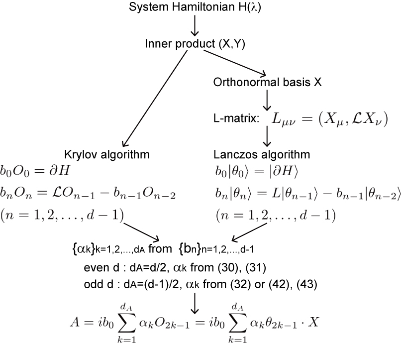
Figure 1: The flowchart of the Krylov algorithm to obtain the AGP $A(\lambda)$ for a given Hamiltonian $H(\lambda)$.

III.4 Operator wave function and adiabatic gauge potential

The AGP is closely related to the operator wave function $\varphi_{n}(\lambda,s)$ defined from the Heisenberg representation

$$e^{iH(\lambda)s}O_{0}(\lambda)e^{-iH(\lambda)s}=\sum_{n=0}^{d-1}i^{n}\varphi_{n}(\lambda,s)O_{n}(\lambda),$$ (58)

where the initial condition is chosen as $b_{0}(\lambda)O_{0}(\lambda)=\partial_{\lambda}H(\lambda)$. Substituting this representation into Eq. (7), we obtain

$$\frac{1}{2}\lim_{\eta\to 0}\int_{-\infty}^{\infty}ds\,{\rm sgn}\,(s)e^{-\eta|s|}\varphi_{2k}(\lambda,s)=0,$$ (59)

for $k=0,1,\dots,d_{A}$, and

$$\frac{1}{2}\lim_{\eta\to 0}\int_{-\infty}^{\infty}ds\,{\rm sgn}\,(s)e^{-\eta|s|}\varphi_{2k-1}(\lambda,s)=(-1)^{k}\alpha_{k}(\lambda),$$

(60)

for $k=1,2,\dots,d_{A}$. This relation between $\varphi_{n}(\lambda,s)$ and $\alpha_{k}(\lambda)$ shows that the latter is obtained from the Laplace transform of the former. The behavior of the operator wave function has been studied in the context of the Krylov complexity, and we can exploit the properties obtained there [63, 64, 65, 66, 67]. For example, the operator wave function $|\varphi(\lambda,s)\rangle=(\varphi_{0},\varphi_{1},\dots,\varphi_{d-1})^{\rm T}$ satisfies the differential equation $\partial_{s}|\varphi(\lambda,s)\rangle=B(\lambda)|\varphi(\lambda,s)\rangle$ with

$$B=\left(\begin{array}[]{cccccc}0&-b_{1}&0&&&\\ b_{1}&0&-b_{2}&&&\\ 0&b_{2}&0&&&\\ &&&\ddots&&\\ &&&&0&-b_{d-1}\\ &&&&b_{d-1}&0\end{array}\right),$$ (67)

and the initial condition $|\varphi(\lambda,0)\rangle=(1,0,0,\dots)^{\rm T}$. $iB$ is related to the matrix $T$ in Eq. (27) under a unitary transformation. Since the equation for $|\varphi(\lambda,s)\rangle$ is interpreted as a Schrödinger equation with a Hamiltonian $iB(\lambda)$ independent of the fictitious time $s$, the solution is obtained by solving the eigenvalue problem $iB(\lambda)|\omega_{n}(\lambda)\rangle=\omega_{n}(\lambda)|\omega_{n}(\lambda)\rangle$. We can write

$$|\varphi(\lambda,s)\rangle=\sum_{n=0}^{d-1}e^{-i\omega_{n}(\lambda)s}|\omega_{n}(\lambda)\rangle\langle\omega_{n}(\lambda)|\varphi(\lambda,0)\rangle.$$ (68)

The form of the Hermitian matrix $iB$ indicates that the eigenvalues come in pairs $\pm\omega_{n}$ where $\omega_{n}\neq 0$, and the zero-eigenvalue state exists only when the size of the matrix $d$ is odd. We refer to the details on the pair eigenstates in Appendix A. Here, we only look at the zero-eigenvalue state $|\phi(\lambda)\rangle$ satisfying $B(\lambda)|\phi(\lambda)\rangle=0$ for odd $d$. We can solve the eigenvalue equation easily to obtain the normalized solution

$$|\phi\rangle=\frac{1}{\sqrt{1+\left(\frac{b_{1}}{b_{2}}\right)^{2}+\cdots}}\left(\begin{array}[]{c}1\\ 0\\ \frac{b_{1}}{b_{2}}\\ 0\\ \frac{b_{3}b_{1}}{b_{4}b_{2}}\\ \vdots\\ \frac{b_{d-2}b_{d-4}\cdots b_{1}}{b_{d-1}b_{d-3}\cdots b_{2}}\end{array}\right).$$ (76)

Since the matrices $L$ and $B$ are constructed from the commutator $\mathcal{L}(\cdot)=[H,(\cdot)]$, the eigenvalues are related to the energy eigenvalue difference $\epsilon_{m}-\epsilon_{n}$. The zero-eigenvalue state of $M$ implies the existence of the diagonal components

$$\partial H-i\mathcal{L}A=\sum_{n}\partial\epsilon_{n}|n\rangle\langle n|.$$ (77)

The contribution on the right-hand side is absent for even $d$ with $\partial\epsilon_{n}=0$.

We can also use the equation for $|\varphi(\lambda,s)\rangle$ to obtain the explicit form of $\alpha_{k}$. The $2k$-th component of the equation is given by $\partial_{s}\varphi_{2k}=b_{2k}\varphi_{2k-1}-b_{2k+1}\varphi_{2k+1}$. Using the integral representation in Eq. (7), we obtain

$$\lim_{\eta\to 0}\int_{0}^{\infty}ds\,e^{-\eta s}\partial_{s}\varphi_{2k}=(-1)^{k}\left(b_{2k}\alpha_{k}+b_{2k+1}\alpha_{k+1}\right).$$

The left-hand side is calculated by using the integration by parts to give

$$\lim_{\eta\to 0}\int_{0}^{\infty}ds\,e^{-\eta s}\partial_{s}\varphi_{2k}=-\delta_{k,0}+\phi_{2k}\phi_{0},$$ (79)

where the second term exists only for odd $d$ and we write $|\phi\rangle=(\phi_{0},\phi_{1},\dots)^{\rm T}$. In the odd-$d$ case, we obtain

$$\alpha_{1}=-\frac{1}{b_{1}}+\frac{\phi_{0}^{2}}{b_{1}},$$ (80)

$$\alpha_{k+1}=-\frac{b_{2k}}{b_{2k+1}}\alpha_{k}+\frac{(-1)^{k}\phi_{2k}\phi_{0}}{b_{2k+1}},$$ (81)

with $k=1,2,\dots,d_{A}-1$. It is not a difficult task to confirm that this relation is consistent with Eq. (57).

The use of the operator wave function also allows us to obtain

$$(A,A)=b_{0}^{2}\sum_{k=1}^{d_{A}}\alpha_{k}^{2}=b_{0}^{2}\langle 0|(QiBQ)^{-2}|0\rangle,$$ (82)

where $|0\rangle=(1,0,\dots,0)^{\rm T}$ and $Q=1-|\phi\rangle\langle\phi|$ represents the projection operator onto the nonzero-eigenvalue states. We show the derivation in Appendix A. This representation is useful when we evaluate the norm of the AGP.

The representation of the AGP by the Lanczos coefficients shows several general properties. For example, we can estimate a contribution from each term of the expansion in Eq. (LABEL:agpk) by the Lanczos coefficient. When $b_{n}$ is an increasing function with respect to $n$, the corresponding $\alpha_{k}$ is a decreasing function. Typical global behaviors of the Lanczos coefficients have been discussed in many-body systems. It was found that $b_{n}\propto n$ for chaotic systems, $b_{n}\propto\sqrt{n}$ for integrable systems, and $b_{n}={\rm const.}$ for noninteracting systems [64]. In Fig. 2, we show the corresponding behaviors of $\alpha_{k}$ for linear and square-root cases. The constant case is found in the examples of Sec. V. In the figure, we also show a special case $b_{n}\propto\sqrt{n(d-n)}$ where the operators defined from the Krylov complexity theory form a SU(2) algebra [64, 65, 66, 67, 68, 69].

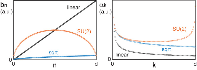
Figure 2: The Lanczos coefficients $b_{n}$ (left panel) and the coefficients of the AGP $\alpha_{k}$ (right panel). We show the cases $b_{n}\propto n$ (linear), $b_{n}\propto\sqrt{n}$ (sqrt), and $b_{n}\propto\sqrt{n(d-n)}$ (SU(2)).

III.5 Classification of basis operators

It is instructive to notice that the AGP consists of the nested commutators at odd orders. When the original Hamiltonian is real symmetric, the nested commutators at even orders $\mathcal{L}^{2k}\partial H$ are real symmetric and those at odd orders $\mathcal{L}^{2k-1}\partial H$ involve the imaginary unit. This means that the basis operators are classified into two parts:

$$X\to(X;Y)=(X_{1},X_{2},\dots,X_{d_{X}};Y_{1},Y_{2},\dots,Y_{d_{Y}}).$$ (83)

$X$ represents basis at even orders and $Y$ at odd orders. These Hermitian operators satisfy $\mathcal{L}X\in Y$ and $\mathcal{L}Y\in X$. Accordingly, the matrix $L$, the basis operator representation of $\mathcal{L}$, takes a form

$$L=\left(\begin{array}[]{cc}0&M\\ M^{\dagger}&0\end{array}\right),$$ (86)

where $M_{\mu\nu}=(X_{\mu},\mathcal{L}Y_{\nu})$. We note that $M_{\nu\mu}^{*}=(Y_{\mu},\mathcal{L}X_{\nu})$. The size of the matrix $M$ is determined by the numbers of the basis operators $d_{X}$ and $d_{Y}=d_{L}-d_{X}$. $M$ is generally a rectangular matrix and the Lanczos algorithm is applied for even $d=2d_{A}$ as

$$M=\left(\begin{array}[]{cccc}|\theta_{0}\rangle&|\theta_{2}\rangle&\cdots&|\theta_{d-2}\rangle\end{array}\right)\left(\begin{array}[]{cccccc}b_{1}&0&0&&&\\ b_{2}&b_{3}&0&&&\\ 0&b_{4}&b_{5}&&&\\ &&&\ddots&&\\ &&&&b_{d-3}&0\\ &&&&b_{d-2}&b_{d-1}\end{array}\right)\left(\begin{array}[]{c}\langle\theta_{1}|\\ \langle\theta_{3}|\\ \vdots\\ \langle\theta_{d-1}|\end{array}\right),$$ (98)

where each of $\{|\theta_{2k}\rangle\}_{k=0}^{d_{A}-1}$ has $d_{X}$ components, each of $\{|\theta_{2k-1}\rangle\}_{k=1}^{d_{A}}$ has $d_{Y}$ components, and the size of the lower triangular matrix on the right-hand side is $d_{A}\times d_{A}$. Since the numbers of the basis operators must be large enough to span the operator space, we find $d_{X}\geq d_{A}$ and $d_{Y}\geq d_{A}$. In the case of odd $d=2d_{A}+1$, $M$ is decomposed as

$$M=\left(\begin{array}[]{cccc}|\theta_{0}\rangle&|\theta_{2}\rangle&\cdots&|\theta_{d-1}\rangle\end{array}\right)\left(\begin{array}[]{cccccc}b_{1}&0&0&&&\\ b_{2}&b_{3}&0&&&\\ 0&b_{4}&b_{5}&&&\\ &&&\ddots&&\\ &&&&b_{d-4}&0\\ &&&&b_{d-3}&b_{d-2}\\ &&&&0&b_{d-1}\end{array}\right)\left(\begin{array}[]{c}\langle\theta_{1}|\\ \langle\theta_{3}|\\ \vdots\\ \langle\theta_{d-2}|\end{array}\right),$$ (111)

where each of $\{|\theta_{2k}\rangle\}_{k=0}^{d_{A}}$ has $d_{X}$ components, each of $\{|\theta_{2k-1}\rangle\}_{k=1}^{d_{A}}$ has $d_{Y}$ components, and the size of the matrix on the right-hand side is $(d_{A}+1)\times d_{A}$. We also find $d_{X}\geq d_{A}+1$ and $d_{Y}\geq d_{A}$. In this case, the minimum number of $d_{X}$ is larger than that of $d_{Y}$.

III.6 Relation to the variational method

The orthonormal relation of operators is useful to understand the relation between the present method and the variational method [39]. In the variational method, the AGP is obtained by minimizing the cost function

$$G[A]={\rm Tr}[\left(\partial H-i{\cal L}A\right)^{2}],$$ (112)

for a given operator ansatz of $A$ with undetermined coefficients. In our notation, this can be written as

$$G[A]=\left(\langle\partial H|+i\langle A|L\right)\left(|\partial H\rangle-iL|A\rangle\right),$$ (113)

with $\rho(H)=1$. One of the systematic methods for obtaining the AGP is to use the nested commutator series in Eq. (8) and carrying out the minimization procedure with respect to the coefficients $\alpha_{k}^{\rm nc}(\lambda)$ [40]. Practically, the number of series elements in Eq. (8) is restricted to a finite value and the approximate AGP is obtained from the minimization.

It is not obvious that the variational method can give the exact AGP even when all of the possible operators are incorporated in the trial form of the AGP by nested commutators. When the AGP satisfies $|\partial H\rangle-iL|A\rangle=0$, which is a sufficient condition of Eq. (16), we have discussed that the Krylov dimension is even and that the matrix $L$ as well as $B$ are invertible. Then, the minimization procedure gives the exact AGP $|A\rangle=-iL^{-1}|\partial H\rangle$.

On the other hand, when the Krylov dimension is odd, $L$ is not invertible and special care is required for the zero-eigenvalue state. The zero-eigenvalue state of $L$ denoted by $|\phi_{L}\rangle$ is obtained in the same way as that of $B$, Eq. (76), and is written by a linear combination of even basis $\{|\theta_{2k}\rangle\}_{k=0}^{(d-1)/2}$. It is orthogonal to the AGP as $\langle\phi_{L}|A\rangle=0$ and the cost function is decomposed as

$$G[A] = \langle\partial H|P|\partial H\rangle$$ (114)

$$+\left(\langle\partial H|Q+i\langle A|L\right)\left(Q|\partial H\rangle-iL|A\rangle\right),$$

where $P=|\phi_{L}\rangle\langle\phi_{L}|$ and $Q=1-P$ are projection operators. The first term does not affect the variational procedure and the minimization of the second term gives

$$|A\rangle=-i(QLQ)^{-1}Q|\partial H\rangle.$$ (115)

This is the solution of $L\left(|\partial H\rangle-iL|A\rangle\right)=0$, which means that the variational method gives the exact AGP.

We note that the trial form of the AGP must include all possible operators from the nested commutators at odd order to find the exact AGP from the variational method. When we consider a restricted number of operators, the minimization gives an approximate AGP. This procedure is equivalent to considering a restricted number of basis operators for the Krylov expansion, as we show in an example in the following section.

A notable remark is that we can find the exact AGP even when we generalize the cost function as

$$G[A]={\rm Tr}[\rho(H)\left(\partial H-i{\cal L}A\right)^{2}].$$ (116)

This form is useful when the dimension of the Hilbert space is infinite and when the spectrum is continuous. Although the exact AGP must be independent of $\rho(H)$, the approximate AGP is generally dependent on it and it is an interesting problem to study how the choice of $\rho(H)$ affects the approximate AGP.

IV Applications to small systems

In the construction of STA, we are basically interested in the time dependence of the Hamiltonian. We set $\lambda(t)=t$ and identify $\lambda$ as time $t$. Then, the AGP is equivalent to the CD term. In the applications discussed below, we write the Hamiltonian as $H(t)$ and use the CD term $H_{\rm CD}(t)$ instead of the AGP $A(\lambda)$. For the small systems to be discussed in the present section, it is not a difficult task to calculate the CD term explicitly. We study how the CD term is obtained by the Krylov method in typical small systems.

IV.1 Two-level system

The study of STA by CD driving in the canonical two-level system [28, 29, 30, 31] was soon followed by its experimental demonstration [19, 24, 76], often in a rotating frame, i.e., making use of a unitarily-equivalent CD Hamiltonian. To illustrate the engineering of STA in Krylov space, consider the two-level Hamiltonian

$$H(t)=\frac{1}{2}h(t)\bm{n}(t)\cdot\bm{\Sigma},$$ (117)

in terms of the positive scalar $h$, the unit vector $\bm{n}=(n_{1},n_{2},n_{3})$, and the vector $\bm{\Sigma}=(X,Y,Z)$ with Pauli operators as entries. In this case, we have essentially no other choices than to set the basis operators as $(X,Y,Z)$. We take the simplest choice $\rho(H)=1/2$ for the inner product. We assume that $\bm{n}(t)$ is dependent on $t$; otherwise, the CD term trivially gives zero. We also know that the parameter dependence of $h(t)$ is not mandatory. $h$ only determines the overall scale of the Hamiltonian and the resulting CD term is independent of $h$.

It is a simple task to calculate the $L$-matrix explicitly. We have

$$L=ih\left(\begin{array}[]{ccc}0&-n_{3}&n_{2}\\ n_{3}&0&-n_{1}\\ -n_{2}&n_{1}&0\end{array}\right).$$ (121)

Then, we set the initial basis vector

$$b_{0}|\theta_{0}\rangle=\frac{\dot{h}}{2}\left(\begin{array}[]{c}n_{1}\\ n_{2}\\ n_{3}\end{array}\right)+\frac{h}{2}\left(\begin{array}[]{c}\dot{n}_{1}\\ \dot{n}_{2}\\ \dot{n}_{3}\end{array}\right),$$ (128)

to generate the Krylov basis

$$O_{0}=\frac{1}{\sqrt{2}}\frac{\dot{h}\bm{n}+h\dot{\bm{n}}}{\sqrt{\dot{h}^{2}+h^{2}\dot{\bm{n}}^{2}}}\cdot\bm{\Sigma},$$ (129)

$$O_{1}=\frac{i}{\sqrt{2}}\frac{\bm{n}\times\dot{\bm{n}}}{|\dot{\bm{n}}|}\cdot\bm{\Sigma},$$ (130)

$$O_{2}=-\frac{1}{\sqrt{2}}\frac{\dot{h}}{|\dot{h}|}\frac{1}{\sqrt{\dot{h}^{2}+h^{2}\dot{\bm{n}}^{2}}}\left(h|\dot{\bm{n}}|\bm{n}-\frac{\dot{h}\dot{\bm{n}}}{|\dot{\bm{n}}|}\right)\cdot\bm{\Sigma},$$

and the Lanczos coefficients

$$b_{1}=\frac{h^{2}|\dot{\bm{n}}|}{\sqrt{\dot{h}^{2}+h^{2}\dot{\bm{n}}^{2}}},$$ (132)

$$b_{2}=\frac{h|\dot{h}|}{\sqrt{\dot{h}^{2}+h^{2}\dot{\bm{n}}^{2}}}.$$ (133)

We find $\mathcal{L}O_{2}-b_{2}O_{1}=0$, which shows $d=3$ and $d_{A}=1$. For $\dot{h}\neq 0$, the Krylov dimension $d=3$ equals the number of basis operators. It is reduced to $d=2$ and $d_{A}=1$ for $\dot{h}=0$ where $b_{2}=0$. We note that the eigenvalues of the Hamiltonian, $\pm h/2$, are time independent when $\dot{h}=0$.

In any case, the dimension of the AGP is given by $d_{A}=1$. We find the CD term

$$H_{\rm CD}=ib_{0}\alpha_{1}O_{1}=-i\frac{b_{0}b_{1}}{b_{1}^{2}+b_{2}^{2}}O_{1}=\frac{1}{2}\bm{n}\times\dot{\bm{n}}\cdot\bm{\Sigma}.$$ (134)

This result is consistent with the known result [28, 29, 30, 31].

IV.2 Driven harmonic quantum oscillator

The driven harmonic oscillator is a workhorse in nonequilibrium quantum dynamics and not surprisingly, has played a key role in the development of STA [12, 77] and their experimental demonstration [16, 26]. Although the dimension of Hilbert space is infinite, it is not difficult to treat the system analytically since the system is a single-particle one, and the spectrum is discrete. In addition, its dynamics is described by a closed Lie algebra [78].

Consider the Hamiltonian

$$H(t)=\frac{1}{2m}P^{2}+\frac{1}{2}m\omega^{2}(t)[Q-q_{0}(t)]^{2}.$$ (135)

where $Q$ and $P$ are the position and momentum operators, respectively. Modulations of the time-dependent frequency $\omega$ induce expansions and compressions while transport processes are associated with variations of the trap center $q_{0}$ [79, 80, 26]. We use the creation-annihilation operator representation

$$H(t)=\omega(t)\left(C^{\dagger}(t)C(t)+\frac{1}{2}\right),$$ (136)

where

$$C(t)=\sqrt{\frac{m\omega(t)}{2}}[Q-q_{0}(t)]+i\sqrt{\frac{1}{2m\omega(t)}}P.$$ (137)

The CD term, in this case, is given by [77, 54, 53]

$$H_{\rm CD} = \dot{q}_{0}P-\frac{\dot{\omega}}{4\omega}\left[P(Q-q_{0})+(Q-q_{0})P\right]$$ (138)

$$= i\dot{q}_{0}\sqrt{\frac{m\omega}{2}}\left(C^{\dagger}-C\right)-i\frac{\dot{\omega}}{4\omega}\left(C^{{\dagger}2}-C^{2}\right).$$

Thus, the CD term involves a term proportional to the momentum operator, the generator of spatial translations, and a second term proportional to the squeezing operator, which is the generator of dilatations.

In the present case, we can explicitly calculate all the nested commutators. As mentioned, using the basis operators $X$ is unnecessary. We find

$$\mathcal{L}^{2k}\dot{H} = -\omega^{2k+1}\sqrt{\frac{m\omega}{2}}\dot{q}_{0}(C^{\dagger}+C)$$

$$+\omega^{2k+1}\frac{2^{2k-1}\dot{\omega}}{\omega}\left(C^{{\dagger}2}+C^{2}\right)+\delta_{k,0}\frac{\dot{\omega}}{\omega}H,$$

for $k=0,1,\dots$, and

$$\mathcal{L}^{2k-1}\dot{H} = -\omega^{2k}\sqrt{\frac{m\omega}{2}}\dot{q}_{0}(C^{\dagger}-C)$$

$$+\omega^{2k}\frac{2^{2(k-1)}\dot{\omega}}{\omega}\left(C^{{\dagger}2}-C^{2}\right),$$

for $k=1,2,\dots$. These nested commutators involve a finite number of operators, which determines the Krylov dimension. It is given by

$$\begin{array}[]{ll}\mbox{$d=5$ and $d_{A}=2$}&\mbox{for $\dot{q}_{0}\neq 0$ and $\dot{\omega}\neq 0$}\\ \mbox{$d=3$ and $d_{A}=1$}&\mbox{for $\dot{q}_{0}=0$ and $\dot{\omega}\neq 0$}\\ \mbox{$d=2$ and $d_{A}=1$}&\mbox{for $\dot{q}_{0}\neq 0$ and $\dot{\omega}=0$}\end{array}.$$ (144)

For $\dot{\omega}=0$, the eigenvalues of the Hamiltonian are time independent and the Krylov dimension is given by an even number. The explicit form of the Krylov basis is given in Appendix B.

It is instructive to see how the exact AGP in Eq. (138) is obtained in the expansion. In the case at $d_{A}=2$, the CD term is expanded as $H_{\rm CD}=H_{\rm CD}^{(1)}+H_{\rm CD}^{(2)}$ and the first term $H_{\rm CD}^{(1)}=ib_{0}\alpha_{1}O_{1}$ is given by

$$H_{\rm CD}^{(1)}=r\dot{q}_{0}P-4r\frac{\dot{\omega}}{4\omega}\left[P(Q-q_{0})+(Q-q_{0})P\right],$$ (145)

where

$$r=\frac{\dot{q}_{0}^{2}z_{1}^{2}+\frac{\dot{\omega}^{2}}{4\omega^{2}}z_{2}^{2}}{\dot{q}_{0}^{2}z_{1}^{2}+\frac{\dot{\omega}^{2}}{\omega^{2}}z_{2}^{2}},$$ (146)

with $z_{1}^{2}={\rm Tr}[\rho(H)P^{2}]$ and $z_{2}^{2}={\rm Tr}[\rho(H)\left(P(Q-q_{0})+(Q-q_{0})P\right)^{2}]$. This result shows that each term of the expansion is dependent on the definition of the inner product in Eq. (9).

IV.3 STIRAP

As a practical application of three-level systems, we next discuss the stimulated Raman adiabatic passage (STIRAP) [81, 82]. It is a method of population transfer between two states. We introduce an additional state and apply two external pump fields to the system. The states are given by $|1\rangle$, $|2\rangle$, and $|3\rangle$ and we consider population transfer between $|1\rangle$ and $|3\rangle$. The simplest STIRAP Hamiltonian is given by

$$H(t)=\frac{1}{2}\left(\begin{array}[]{ccc}0&\omega_{p}(t)&0\\ \omega_{p}(t)&2\delta&\omega_{s}(t)\\ 0&\omega_{s}(t)&0\end{array}\right).$$ (150)

A typical protocol is given in Fig. 3.

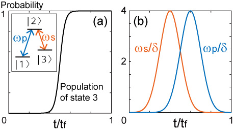
Figure 3: (a) Schematic view of STIRAP. Three-level states are driven by two kinds of pulses, shown in the inset, and the initial state $|1\rangle$ is adiabatically transferred to $|3\rangle$. (b) A typical protocol for STIRAP. We set $\omega_{s}(t)=\omega_{0}\exp\left[-(t-t_{1})^{2}/2\sigma^{2}\right]$ and $\omega_{p}(t)=\omega_{0}\exp\left[-(t-t_{2})^{2}/2\sigma^{2}\right]$ with $\omega_{0}/\delta=4.0$, $\delta t_{\rm f}=100$, $t_{1}/t_{\rm f}=0.4$, $t_{2}/t_{\rm f}=0.6$, and $\sigma/t_{\rm f}=0.1$.

Since we treat three-level systems, the number of independent operators are given by eight, except the identity operator. We also see that the Hamiltonian is real symmetric and the $L$-matrix is written as Eq. (86). Possible basis operators for $\rho(H)=1/2$ are given by

$$X = \left\{\left(\begin{array}[]{ccc}0&1&0\\ 1&0&0\\ 0&0&0\end{array}\right),\left(\begin{array}[]{ccc}0&0&0\\ 0&0&1\\ 0&1&0\end{array}\right),\left(\begin{array}[]{ccc}0&0&1\\ 0&0&0\\ 1&0&0\end{array}\right),\right.$$ (167)

$$\left.\left(\begin{array}[]{ccc}1&0&0\\ 0&-1&0\\ 0&0&0\end{array}\right),\frac{1}{\sqrt{3}}\left(\begin{array}[]{ccc}1&0&0\\ 0&1&0\\ 0&0&-2\end{array}\right)\right\},$$

and

$$Y=\left\{\left(\begin{array}[]{ccc}0&-i&0\\ i&0&0\\ 0&0&0\end{array}\right),\left(\begin{array}[]{ccc}0&0&0\\ 0&0&-i\\ 0&i&0\end{array}\right),\left(\begin{array}[]{ccc}0&0&-i\\ 0&0&0\\ i&0&0\end{array}\right)\right\}.$$ (177)

Using this basis, we find Eq. (86) with

$$M=i\left(\begin{array}[]{ccc}\delta&0&\omega_{s}/2\\ 0&-\delta&-\omega_{p}/2\\ \omega_{s}/2&-\omega_{p}/2&0\\ \omega_{p}&-\omega_{s}/2&0\\ 0&\sqrt{6}\omega_{s}/2&0\end{array}\right).$$ (184)

We note that the number of operators in $X$ can be reduced to four, as we can understand from the general discussions in the previous section. Since they are not much different, we use the $5\times 3$ matrix here.

We apply the Lanczos algorithm for the given $M$-matrix with the protocol in Fig. 3(b) to calculate $\alpha_{k}$ shown in Fig. 4(a). The Krylov dimension is given by $d=7$.

The expansion is compared with the exact result [83]

$$H_{\rm CD}(t)=-\dot{\phi}(t)\sin\theta(t)Y_{1}+\dot{\phi}(t)\cos\theta(t)Y_{2}-\dot{\theta}(t)Y_{3},$$

where $\theta(t)=\arctan(\omega_{p}(t)/\omega_{s}(t))$ and $\phi(t)=[\arctan(\sqrt{\omega_{p}^{2}(t)+\omega_{s}^{2}(t)}/\delta)]/2$. In the Krylov method, the CD term is given by the form $H_{\rm CD}(t)=ib_{0}\sum_{k=1}^{3}\alpha_{k}O_{2k-1}$. When we rewrite it as $H_{\rm CD}(t)=\sum_{\mu=1}^{3}a_{\mu}Y_{\mu}$, the coefficients are written as $a_{\mu}=\sum_{k=1}^{3}a_{\mu}^{(k)}$ where

$$a_{\mu}^{(k)}=ib_{0}\alpha_{k}(Y_{\mu},O_{2k-1}),$$ (186)

and are plotted in Fig. 4(b)–(d). For short and large times, the adiabatic condition is approximately satisfied and the CD term is well approximated by the first term of the Krylov expansion.

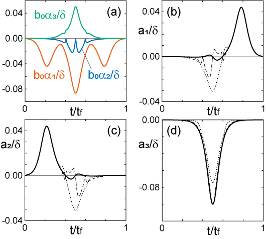
Figure 4: (a) Coefficients of the CD term $\alpha_{k}$ for STIRAP. (b)–(d) $a_{\mu}^{(1)}$ (dotted curves), $a_{\mu}^{(1)}+a_{\mu}^{(2)}$ (dashed curves), and $a_{\mu}=\sum_{k=1}^{3}a_{\mu}^{(k)}$ (solid curves).

V Applications to many-body systems

The exact AGP/CD term is known for a limited number of many-body systems and we expect that the Krylov method gives advantageous results that cannot be obtained from other methods. For many-body systems, the required number of operators is large and it is still a formidable task to find the exact CD term even in the present method. In this section, we treat one-dimensional spin systems where the exact CD term is known for some examples.

V.1 One-dimensional transverse Ising model

V.1.1 Exact result without longitudinal magnetic field

We first treat the Ising spin chain in a transverse field:

$$H(t)=-\frac{v}{2}\left(\sum_{n=1}^{n_{s}}X_{n}X_{n+1}+g(t)\sum_{n=1}^{n_{s}}Z_{n}\right).$$ (187)

Many spins are aligned in a chain and the number of spins is denoted by $n_{s}$. We consider the periodic boundary condition and the subscript is interpreted as ${\rm mod}\,n_{s}$. We are interested in the large-$n_{s}$ limit where the system at $g=1$ shows a quantum phase transition [84, 85].

It is also known that the system is equivalent to the free fermion system [86, 87]. Then, the Hamiltonian is represented as an ensemble of two-level systems and the CD term for each two-level system can be found from the result in the previous section. Here, to study properties for many-body systems, we do not use the mapping and treat the spin operators.

Under the setting $\rho(H)=1/(2^{n_{s}}n_{s})$, we define orthonormalized operators

$$M=\sum_{n=1}^{n_{s}}Z_{n},$$ (188)

$$V_{k}^{X}=\sum_{n=1}^{n_{s}}X_{n}Z_{n+1}\cdots Z_{n+k-1}X_{n+k},$$ (189)

$$V_{k}^{Y}=\sum_{n=1}^{n_{s}}Y_{n}Z_{n+1}\cdots Z_{n+k-1}Y_{n+k},$$ (190)

$$W_{k}=\frac{1}{\sqrt{2}}\sum_{n=1}^{n_{s}}\left(X_{n}Z_{n+1}\cdots Z_{n+k-1}Y_{n+k}\right.$$

$$\left.+Y_{n}Z_{n+1}\cdots Z_{n+k-1}X_{n+k}\right),$$ (191)

with $k=1,2,\dots,n_{s}-1$. These operators take bilinear forms in fermion operators and can be used as basis operators. Since the Hamiltonian commutes with $(-1)^{P}=\prod_{n=1}^{n_{s}}Z_{n}$, the number of independent operators are reduced. We have the relations $V_{n-k}^{X}=-(-1)^{P}V_{k}^{Y}$, $V_{n-k}^{Y}=-(-1)^{P}V_{k}^{X}$, and $W_{n-k}=(-1)^{P}W_{k}$. Then, the subscript takes $k=1,2,\dots,n_{s}/2$ for even $n_{s}$.

Acting $\mathcal{L}$ to these operators, we obtain

$$\mathcal{L}M=\sqrt{2}ivW_{1},$$ (192)

$$\mathcal{L}V_{k}^{X}=\sqrt{2}iv\left(W_{k-1}-gW_{k}\right),$$ (193)

$$\mathcal{L}V_{k}^{Y}=\sqrt{2}iv\left(-W_{k+1}+gW_{k}\right),$$ (194)

$$\mathcal{L}W_{k}=\sqrt{2}iv\left[V_{k-1}^{X}-V_{k+1}^{Y}+g(V_{k}^{X}-V_{k}^{Y})-\delta_{k,1}M\right].$$

Since the Hamiltonian is real symmetric, the nested commutators at odd order only involve $W_{k}$. In Appendix C, we show

$$O_{2k-1}=(-1)^{k}iW_{k},$$ (196)

and

$$b_{1}^{2}+b_{2}^{2}=b_{3}^{2}+b_{4}^{2}=\cdots=b_{d-2}^{2}+b_{d-1}^{2}=4v^{2}(1+g^{2}),$$

(197)

$$b_{2}b_{3}=b_{4}b_{5}=\cdots=b_{d-3}b_{d-2}=4v^{2}g.$$ (198)

The Krylov dimension is odd in this case. Using the result $b_{0}=\sqrt{n_{s}}v\dot{g}(t)/2$ and $b_{1}=\sqrt{2}v$, where we assume $v>0$ and $\dot{g}(t)>0$, we can calculate all of the Lanczos coefficients. We plot the Lanczos coefficients in the left panels of Fig. (5) for several values of $g$. The asymptotic forms satisfy $b_{2k}\sim 2v\geq b_{2k-1}\sim 2vg$ for $g\leq 1$ and $b_{2k}\sim 2vg\geq b_{2k-1}\sim 2v$ for $g\geq 1$. This result implies that we can generally find a phase transition point from the Lanczos coefficients.

The coefficients of the CD term are obtained from Eq. (57). Since the matrix in the equation has the diagonal components $4v^{2}(1+g^{2})$ and the nonzero offdiagonal components $4v^{2}g$, we can invert the matrix by using the discrete Fourier transformation. The details are given in Appendix C. We obtain

$$(-1)^{k-1}b_{0}\alpha_{k}=\dot{g}\sqrt{\frac{n_{s}}{2}}\frac{1}{2(d_{A}+1)}$$

$$\times\sum_{l=1}^{d_{A}}\frac{\sin\frac{\pi l}{d_{A}+1}}{1+g^{2}-2g\cos\frac{\pi l}{d_{A}+1}}\sin\frac{k\pi l}{d_{A}+1}.$$ (199)

The CD term is given by $H_{\rm CD}=\sum_{k=1}^{d_{A}}(-1)^{k-1}b_{0}\alpha_{k}W_{k}$ with $d_{A}=n_{s}/2$. This result entirely agrees with that in [38, 48]. Since the Krylov basis at odd order in the present case is given by a simple form $W_{k}$, it is natural to find the same result without using the Krylov method.

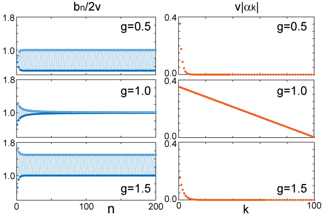
Figure 5: The Lanczos coefficients (left panels) and the coefficients of the CD term (right panels) for the one-dimensional transverse Ising model in Eq. (187) at $n_{s}=200$. For the Lanczos coefficients, we denote $b_{1},b_{3},\dots$ by the filled circle $\bullet$ and $b_{2},b_{4},\dots$ by the open circle $\circ$.

We plot $\alpha_{k}$ for several values of $g$ in the right panels of Fig. 5. For $g\neq 1$, the Lanczos coefficients at even order are larger than those at odd order, we see from Eq. (81) that $\alpha_{k}$ is a decreasing function in $k$. Then, we find that $\alpha_{k}$ rapidly decreases, which means that few-body interactions become the dominant contributions to the CD term. It was discussed in [38, 88] that $\alpha_{k}\sim g^{k-1}$ for $|g|<1$ and $\alpha_{k}\sim g^{-k-1}$ for $|g|>1$ at the thermodynamic limit $n_{s}\to\infty$. For $g=1$, the Lanczos coefficients take a constant value and $\alpha_{k}$ decreases slowly as a function of $k$. At $n_{s}\to\infty$, an infinite number of operators contributes to the CD term as discussed in [38].

V.1.2 Approximate result with longitudinal magnetic field

The free fermion representation is possible only when the direction of the magnetic field is perpendicular to the direction of the interaction operator. Here, we treat the nonintegrable Hamiltonian

$$H(t) = g(t)\left(-v\sum_{n=1}^{n_{s}}Z_{n}Z_{n+1}-h\sum_{n=1}^{n_{s}}Z_{n}\right)$$ (200)

$$+(1-g(t))\left(-\gamma\sum_{n=1}^{n_{s}}X_{n}\right),$$

with $g(t)=t/t_{\rm f}$. This is the standard form of the quantum annealing Hamiltonian and a test-bed for universal dynamics of quantum phase transitions with a bias [89]. We consider the time evolution from the ground state of $H(0)$ toward that of $H(t_{\rm f})$. The nonadiabatic effect makes the system deviate from the instantaneous ground state, and we apply the CD term to prevent the transition.

It is a complex problem to find and implement the exact CD term for this Hamiltonian and we consider a restricted number of operators. As we discussed in the above example, each term of $H_{\rm CD}(t)$ involves an odd number of Pauli $Y$ operators. We keep the $Y$-basis up to two-body operators

$$Y = \left(\sum_{n=1}^{n_{s}}Y_{n},\ \frac{1}{\sqrt{2}}\sum_{n=1}^{n_{s}}\left(Y_{n}Z_{n+1}+Z_{n}Y_{n+1}\right),\ \right.$$ (201)

$$\frac{1}{\sqrt{2}}\left.\sum_{n=1}^{n_{s}}\left(Y_{n}X_{n+1}+X_{n}Y_{n+1}\right)\right),$$

with $\rho(H)=1/(2^{n_{s}}n_{s})$. We act with ${\cal L}$ on these operators to construct the $M$-matrix. Using the $X$-basis

$$X=\left(\sum_{n=1}^{n_{s}}Z_{n},\ \sum_{n=1}^{n_{s}}X_{n},\ \sum_{n=1}^{n_{s}}Z_{n}Z_{n+1},\ \right.$$

$$\sum_{n=1}^{n_{s}}X_{n}X_{n+1},\ \sum_{n=1}^{n_{s}}Y_{n}Y_{n+1},$$

$$\frac{1}{\sqrt{2}}\sum_{n=1}^{n_{s}}\left(Z_{n}X_{n+1}+X_{n}Z_{n+1}\right),\ \sum_{n=1}^{n_{s}}Z_{n-1}X_{n}Z_{n+1},$$

$$\frac{1}{\sqrt{2}}\sum_{n=1}^{n_{s}}\left(Z_{n-1}X_{n}X_{n+1}+X_{n-1}X_{n}Z_{n+1}\right),$$

$$\frac{1}{\sqrt{2}}\left.\sum_{n=1}^{n_{s}}\left(Z_{n-1}Y_{n}Y_{n+1}+Y_{n-1}Y_{n}Z_{n+1}\right)\right),$$ (202)

we can construct the $M$-matrix with the size $9\times 3$ and apply the Lanczos algorithm to calculate the approximate CD term. We note that the size of the $M$-matrix can be reduced to $3\times 3$ keeping the result unchanged. The Krylov dimension is given by $d=7$.

We calculate the approximate CD term and numerically solve the time evolution with and without the approximate CD term by setting the initial state as the ground state of $H(0)$ for the system size $N=6$. In Fig.  6, we plot the approximate CD term as a function of $t$ and the fidelity

$$f=|\langle\psi_{\rm gs}(t_{\rm f})|\psi(t_{\rm f})\rangle|^{2},$$ (203)

as a function of the annealing time $t_{\rm f}$. Here, $|\psi(t)\rangle$ represents the time-evolved state with or without the approximate CD term and $|\psi_{\rm gs}(t)\rangle$ represents the instantaneous ground state of $H(t)$. $f$ is close to unity when the adiabaticity condition is satisfied.

We numerically confirm that the present method gives the same result as the variational method, which is expected from the general discussion. When $h/v$ takes a large value, the ground-state energy is well-separated from the other ones, and we find a large fidelity. As $h/v$ decreases to zero, the fidelity becomes smaller and finding the exact ground state becomes difficult even with the approximate CD term in use. As we see from the figure, many-body terms in the CD term become important for small $h$ and we require higher-order terms to improve the result by the approximate CD driving.

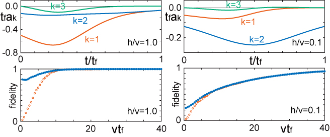
Figure 6: The time evolution for the quantum annealing Hamiltonian in Eq. (200). We set $N=6$, $\gamma/v=1.0$, $h/v=1.0$ for the left panels, and $h/v=0.1$ for the right panels. In the upper panels, we plot $(a_{1}(t),a_{2}(t),a_{3}(t))$ for the approximate CD term $H_{\rm CD}(t)=a_{1}(t)Y_{1}+\sqrt{2}a_{2}(t)Y_{2}+\sqrt{2}a_{3}(t)Y_{3}$. In the lower panels, we plot the fidelity $f$ for the time evolutions with $H(t)$ (red open circle $\circ$) and with $H(t)+H_{\rm CD}(t)$ (blue filled circle $\bullet$).

V.2 One-dimensional XX model

V.2.1 Krylov method

In the example of the Hamiltonian in Eq. (187), $O_{2k-1}$ incorporates $k+1$-body interactions only, which is a specific property for the transverse Ising model. Here, to study more complicated situations, we treat the one-dimensional isotropic XY model (XX model) with the open boundary condition

$$H(t) = \frac{1}{2}\sum_{n=1}^{n_{s}-1}v_{n}(t)(X_{n}X_{n+1}+Y_{n}Y_{n+1})$$ (204)

$$+\frac{1}{2}\sum_{n=1}^{n_{s}}h_{n}(t)Z_{n}.$$

This model is also known to be equivalent to a free fermion model. However, the coefficients are dependent on the site index $n$ and it is generally a difficult task to find the exact CD term.

The mapping to a bilinear form in fermion operators denotes that we can find a closed algebra within a limited number of operators. For $\rho(H)=1/2^{n_{s}}$, we define

$$V_{n}^{k}=\frac{1}{\sqrt{2}}\left(X_{n}Z_{n+1}\cdots Z_{n+k-1}X_{n+k}\right.$$

$$\left.+Y_{n}Z_{n+1}\cdots Z_{n+k-1}Y_{n+k}\right),$$ (205)

$$W_{n}^{k}=\frac{1}{\sqrt{2}}\left(X_{n}Z_{n+1}\cdots Z_{n+k-1}Y_{n+k}\right.$$

$$\left.-Y_{n}Z_{n+1}\cdots Z_{n+k-1}X_{n+k}\right),$$ (206)

with $n=1,2,\dots,n_{s}$ and $k=1,2,\dots,n_{s}-n$. Since the Hamiltonian is real symmetric, we define $X=(\{Z_{n}\},\{V_{n}^{k}\})$ and $Y=(\{W_{n}^{k}\})$ to construct the $M$-matrix with the size $n_{s}(n_{s}+1)/2\times n_{s}(n_{s}-1)/2$. We have

$$\mathcal{L}W_{n}^{k}=-i(h_{n+k}-h_{n})V_{n}^{k}-iv_{n-1}V_{n-1}^{k+1}-iv_{n}V_{n+1}^{k-1}$$

$$+iv_{n+k-1}V_{n}^{k-1}+iv_{n+k}V_{n}^{k+1}$$

$$+\delta_{k,1}\sqrt{2}iv_{n}(Z_{n+1}-Z_{n}).$$ (207)

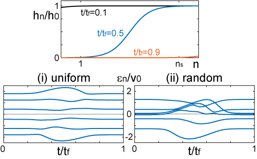
Figure 7: The protocol for the XX model in Eq. (204). The upper panel represents $h_{n}(t)$. We take $h_{n}(t)=h_{0}(1+\tanh f_{n}(t))/2$, $f_{n}(t)=n-1+x_{0}-(n_{s}-1+2x_{0})t/t_{\rm f}$ with $x_{0}=4$ and $n_{s}=6$. The lower panels represent the instantaneous eigenvalues of the Hamiltonian for the uniform case (i) and the random case (ii) with $h_{0}/v_{0}=2.0$. In the following calculations, we take $v_{0}t_{\rm f}=100$.

For the Hamiltonian coefficients $\{v_{n}(t)\}_{n=1}^{n_{s}-1}$ and $\{h_{n}(t)\}_{n=1}^{n_{s}}$, we consider an annealing protocol. We take $v_{n}$ as a constant value and consider the two cases: (i) uniform distribution $v_{n}=v_{0}>0$, and (ii) random distribution $v_{n}=v_{0}r_{n}$ where $r_{n}$ is a uniform random number with $r_{n}\in[-1,1]$. For a given set of $\{v_{n}\}$, we change the magnetic field $h_{n}(t)$ from $h_{n}(0)=h_{0}\gg|v_{n}|$ to $h_{n}(t_{\rm f})=0$. We take $h_{n}(t)=h_{0}(1+\tanh f_{n}(t))/2$ with $f_{n}(t)=n-1+x_{0}-(n_{s}-1+2x_{0})t/t_{\rm f}$. The system becomes adiabatic for large $t_{\rm f}$. The parameter $x_{0}$ takes a large value so that the conditions at $t=0$ and $t=t_{\rm f}$ are satisfied. We plot the protocols used in the following calculations in the upper panel of Fig. 7. The instantaneous eigenvalues for (i) and (ii) are respectively plotted in the lower panels of Fig. 7. The Hamiltonian commutes with $M=\sum_{n=1}^{n_{s}}Z_{n}$ and we consider the block with $M=n_{s}-2$. The Hamiltonian takes a tridiagonal form and the size of the matrix is given by $n_{s}$.

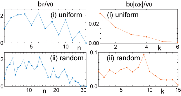
Figure 8: The Lanczos coefficients, $b_{n}$, and the coefficients of the CD term, $\alpha_{k}$, for the XX model with $n_{s}=6$ at $t/t_{\rm f}=0.5$. The top panels are results for the case (i), uniform distribution, and the bottom panels are for (ii), random distribution. For the Lanczos coefficients, we denote $b_{1},b_{3},\dots$ by the filled circle $\bullet$ and $b_{2},b_{4},\dots$ by the open circle $\circ$.

Although it is not difficult to implement the Lanczos algorithm numerically for a considerably large value of $n_{s}$, we here take $n_{s}=6$ to keep a good visibility of the plotted points. In Fig. 8, we display the Lanczos coefficients and the coefficients of the CD term for a fixed $t$. The Lanczos coefficients show an oscillating behavior. For the uniform case (i), the even order tends to be larger than the odd order, and correspondingly $|\alpha_{k}|$ shows a decreasing behavior. For the random case (ii), we observe a complicated behavior denoting that the higher-order contributions of the Lanczos expansion are important.

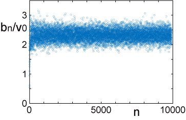
Figure 9: The Lanczos coefficients of the XX model with $n_{s}=100$. We consider the random case (ii) and take $t/t_{\rm f}=0.5$.

The typical behavior of $b_{n}$ for a large $n_{s}$ is shown in Fig. 9. For any choice of parameters, we observe a flat band, which is considered to be a property for “noninteracting” systems.

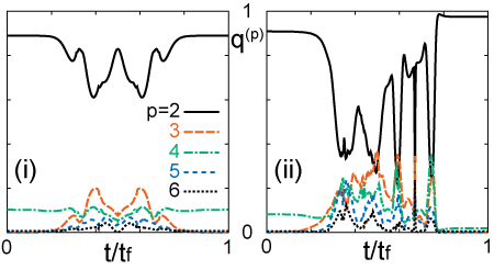
Figure 10: Time dependence of the norm fraction $\{q^{(p)}(t)\}_{p=2}^{n_{s}}$ in Eq. (213), weighting the contribution of the $p$-body interactions to the CD term, for the XX model with $n_{s}=6$. Many-body CD terms are shown to be necessary when the energy levels change significantly along the driving protocol.

To study the properties of the obtained CD term, we next decompose it. The Lanczos basis at odd order is written as

$$|\theta_{2k-1}\rangle=\left(\begin{array}[]{cc}|\theta_{2k-1}^{(2)}\rangle\\ |\theta_{2k-1}^{(3)}\rangle\\ \vdots\\ |\theta_{2k-1}^{(n_{s})}\rangle\end{array}\right),$$ (212)

where $|\theta_{2k-1}^{(p)}\rangle$ has $n_{s}+1-p$ components and the corresponding Krylov basis involves $p$-body interactions. We decompose the norm of the CD term as $\langle H_{\rm CD}|H_{\rm CD}\rangle=\sum_{p=2}^{n_{s}}\langle H_{\rm CD}^{(p)}|H_{\rm CD}^{(p)}\rangle$ where $|H_{\rm CD}^{(p)}\rangle=-b_{0}\sum_{k=1}^{d_{A}}\alpha_{k}|\theta_{2k-1}^{(p)}\rangle$, and define the norm fraction

$$q^{(p)}=\frac{\langle H_{\rm CD}^{(p)}|H_{\rm CD}^{(p)}\rangle}{\langle H_{\rm CD}|H_{\rm CD}\rangle}=\frac{\sum_{k=1}^{d_{A}}\alpha_{k}^{2}\langle\theta_{2k-1}^{(p)}|\theta_{2k-1}^{(p)}\rangle}{\sum_{k=1}^{d_{A}}\alpha_{k}^{2}},$$ (213)

which weights the contribution of the $p$-body term. This is a function of $t$ and is plotted for each value of $p$ in Fig. 10. We can understand from the comparison between the energy levels in Fig. 7 and $q^{(p)}$ in Fig. 10 that the many-body interaction terms cannot be neglected when the energy levels significantly change as a function of $t$.

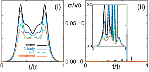
Figure 11: The norm of the CD term for the XX model at $n_{s}=6$. Bold solid curves ”exact” (black) represent $\sigma=\sqrt{\langle H_{\rm CD}|H_{\rm CD}\rangle}$. We use the replacement $H_{\rm CD}\to H_{\rm CD}^{(2)}$ for dashed curves ”2-body” (blue), $H_{\rm CD}\to ib_{0}\alpha_{1}O_{1}$ for dotted curves ”$k=1$” (green), and $H_{\rm CD}\to i\alpha_{1}^{\rm nc}\mathcal{L}\dot{H}$ for thin solid curves ”variational” (red) where $\alpha_{1}^{\rm nc}$ is obtained from the variational method.

It is generally understood from Eq. (5) that the CD term gives a large contribution when some of the energy levels are close to each other. We calculate the amplitude of the CD term $\langle H_{\rm CD}|H_{\rm CD}\rangle$ which is plotted in Fig. 11. As we have discussed, the CD term is decomposed as $H_{\rm CD}=\sum_{p}H_{\rm CD}^{(p)}$ and $H_{\rm CD}=ib_{0}\sum_{k}\alpha_{k}O_{2k-1}$. In the same figure, we plot the result where the first term of the expansion is kept for each decomposition. We also plot the first contribution of the approximate CD term $H_{\rm CD}^{\rm nc}$ obtained from the expansion in Eq. (8). The coefficient $\alpha_{1}^{\rm nc}$ is obtained from the minimization condition of ${\rm Tr}[(\dot{H}-i\mathcal{L}H_{\rm CD}^{\rm nc})^{2}]$ [39, 40]. The result implies that the approximate CD term underestimates an abrupt growth of the CD term.

We note that this result does not necessarily lead to the failure of the approximation method. The CD term is independent of the choice of the initial condition of the time evolution. In the present examples, as we see from Fig. 7, the energy level crossings occur at higher energy levels. The ground-state level is isolated from the other levels, and we can expect that a large amplitude of the CD term is not required for the control of the ground state. The situation is, in this sense, opposite to that across a quantum phase transition, discussed in Sec. V.1.1, in which the gap between the ground state and the first excited state closes, and the norm of the CD exhibits a singularity [38, 88].

In the present analysis, we set the measure $\rho(H)$ in the inner product as $\rho(H)=1/2^{n_{s}}$. When we control a state with an energy level well separated from the other levels, it is reasonable to consider a weighted measure such as the Gibbs–Boltzmann distribution $\rho(H)\propto e^{-\beta H}$. Although the exact CD term is independent of the measure, each term of the expansion $H_{\rm CD}=ib_{0}\sum_{k=1}^{d_{A}}\alpha_{k}O_{2k-1}$ is dependent on it. Therefore, when we consider a truncation approximation in the Krylov expansion, the choice of the measure strongly influences the result. Since a nontrivial choice of the measure makes the calculation of the inner product difficult, it is practically an interesting problem to find a convenient form of the measure. For the ground state, it is tempting to take the limit $\beta\to\infty$ for $\rho(H)\propto e^{-\beta H}$. However, the measure is not positive definite in this limit and we will find unexpected behavior, such as the vanishing of the Lanczos coefficient $b_{n}$ for $n<d-1$.

V.2.2 Toda equation

It is known that the exact CD term is analytically obtained when the coefficients of the Hamiltonian satisfy the Toda equations [90]

$$\dot{h}_{n}(t)=2[v_{n}^{2}(t)-v_{n-1}^{2}(t)],$$ (214)

$$\dot{v}_{n}(t)=v_{n}(t)[h_{n+1}(t)-h_{n}(t)].$$ (215)

The CD term is then given by

$$H_{\rm CD}(t)=\frac{1}{\sqrt{2}}\sum_{n=1}^{n_{s}-1}v_{n}(t)W_{n}^{1},$$ (216)

with $W_{n}^{1}$ as in Eq. (206). This term satisfies $\dot{H}-i\mathcal{L}H_{\rm CD}=0$, which means that the instantaneous eigenvalues of the Hamiltonian are time-independent.

Despite this simplicity, the corresponding Krylov expansion is generally involved and is required at each time. The time evolution of the Hamiltonian is only reflected in the choice of the initial basis $b_{0}O_{0}=\dot{H}$ and the expansion is essentially insensitive to the choice. Except for the special cases discussed below, we find that the Krylov dimension is as large as the number of odd basis elements $n_{s}(n_{s}-1)/2$. Highly nontrivial cancellations should be observed when we calculate $\alpha_{k}$ to give the result with $q^{(p)}=\delta_{p,2}$.

As a very special case, we can find the result with $d=2$ and $d_{A}=1$ when the coefficients are written as

$$h_{n}(t)=-\frac{2h_{1}}{n_{s}-1}\left(n-\frac{n_{s}+1}{2}\right)\sin\theta(t),$$ (217)

$$v_{n}^{2}(t)=\frac{n(n_{s}-n)}{(n_{s}-1)^{2}}h_{1}^{2}\cos^{2}\theta(t).$$ (218)

Using the Toda equations, we obtain that a single equation describes the time evolution

$$\frac{\dot{\theta}(t)}{\cos\theta(t)}=\frac{2h_{1}}{n_{s}-1}.$$ (219)

For a given $h_{1}$ and a initial condition $\theta(0)$, the coefficients evolve, keeping the equidistant of $h_{n}(t)$ and a quadratic form of $v_{n}(t)$. In this case, we find that the first-order term in the Krylov expansion is proportional to the exact CD term, i.e.,

$$b_{0}b_{1}O_{1}=\mathcal{L}\dot{H}(t)=\frac{i}{\sqrt{2}}\left(\frac{2h_{1}}{n_{s}-1}\right)^{2}\sum_{n=1}^{n_{s}-1}v_{n}(t)W_{n}^{1}.$$ (220)

Since $\mathcal{L}O_{1}-b_{1}O_{0}=0$, the expansion terminates at this order and we obtain a simple result with $d=2$.

It was discussed that the present choice of parameters saturates the operator speed limit, i.e., the quantum speed limit in unitary operator flows  [69]. The nested commutators span the Krylov space within a limited number of operators.

VI Discussion and Summary

The use of the integral representation of the CD term introduced in [40] has eased the study of STA in many-body systems by removing the requirement for the exact diagonalization of the instantaneous system Hamiltonian. In its place, the CD term can be expressed as a series that follows from the Baker–Campbell–Hausdorff formula. The coefficients in such an expansion can be determined through a variational principle [39].

In this work, we have introduced Krylov subspace methods to provide an exact expression of the CD term. The Krylov algorithm identifies an operator basis for the terms generated in the series by nested commutators, along with the set of Lanczos coefficients. Using these two ingredients, we have provided an exact closed-form expression of the CD term circumventing the need for a variational approach. When the dimension of the Hilbert space is finite, the series by the Krylov basis is finite, which is in contrast to the expansion using nested commutators.

We have shown the applicability of our method in the paradigmatic models in which the CD term admits an exact closed-form solution. This includes single-particle systems such as two- and three-level systems and the driven quantum oscillator. Although the applications of the present method to those simple systems requires some tedious calculations, the implementation is a straightforward task and is applied to any Hamiltonian with no special symmetry. We have further applied our formalism to a variety of quantum spin chain models encompassing the cases in which the system is integrable, nonintegrable, and disordered. Specifically, we applied the construction of the CD term in Krylov space to the one-dimensional transverse-field quantum Ising model as a paradigmatic instance of an integrable and solvable quasi-free fermion Hamiltonian. We have further demonstrated our approach in the presence of a longitudinal symmetry-breaking bias field that breaks integrability. A similar study is possible for the XX model where the free fermion representation is available. However, in that case, the site-dependent couplings make the explicit construction of the CD term by the standard method difficult, except for the special case when the coupling constants are varied in time according to a Toda flow, and the resulting CD term takes a simple local form. We have explicitly constructed the CD term for general and disordered couplings and the result was compared to the approximation method [39, 40].

The main task of the Krylov algorithm is to construct the basis operators for the minimal subspace in which the dynamics unfolds and to determine the associated Lanczos coefficients by iterations. The CD term is constructed as a series involving only the odd-order operators of the Krylov basis, with the corresponding coefficients in this compact expansion being determined in terms of the Lanczos coefficients. These properties imply that we can find some implications by comparing the Lanczos coefficients of odd order and those of even order. As we see from Figs. 5 and 8, the Lanczos coefficients typically show an oscillating behavior. When the coefficients at even order are larger than those at odd order, the corresponding coefficients of the CD term show a decaying behavior, and the CD term is well approximated by the first several terms of the expansion. We also find that the Krylov dimension is even when the instantaneous eigenstates of the original Hamiltonian are time-independent. Thus, we can directly find the dynamical properties of the system from the Krylov algorithm.

The Krylov expansion is dependent on the choice of the inner product. Although the CD term is independent of the choice, each term in Eq. (LABEL:agpk) is sensitive to it, a feature that can be relevant when considering truncating approximations. It is an interesting problem to find a proper choice depending on the situation to treat. We can also consider the truncation of the Krylov subspace. To this end, it suffices to restrict the basis operators and to construct the $L$-matrix in the truncated space. Then, we can apply the Lanczos algorithm to find an approximate CD term. This method is shown to be equivalent to the variational method.

To summarize, we have proposed a technique for constructing the CD term exploiting the Krylov operator space. The method is flexibly applied to systems with many degrees of freedom and can be a powerful general method for understanding the dynamical properties of the system in control. Suppression of nonadiabatic transitions in discrete systems with many degrees of freedom is one of the dominant problems in quantum computing, and we hope that our method will be an efficient technique in further studies. In particular, our formulation of STA suggests a new class of quantum algorithms based on digitized CD driving in Krylov space, with the potential to outperform the state-of-the-art.

Appendix A Derivation of Eq. (82)

In Sec. III.4, we discussed the relation between the AGP and the operator wave function $|\varphi(s)\rangle$. The wave function satisfies $\partial|\varphi(s)\rangle=B|\varphi(s)\rangle$ with the matrix $B$ in Eq. (67) and the initial condition $|\varphi(0)\rangle=(1,0,0,\dots)^{\rm T}$. Since $B$ is independent of $s$, we can solve the differential equation by the standard method for stationary states. Since $iB$ is Hermitian, the eigenvalue equation

$$iB|\omega_{n}\rangle=\omega_{n}|\omega_{n}\rangle$$ (221)

is solved to find a real eigenvalue $\omega_{n}$. We also find that $B$ anticommutes with $Z={\rm diag}\,(1,-1,1,-1,\dots)$, which gives the relation

$$iBZ|\omega_{n}\rangle=-\omega_{n}Z|\omega_{n}\rangle.$$ (222)

This identity shows that, for the eigenstate $|\omega_{n}\rangle$ with the eigenvalue $\omega_{n}$, $Z|\omega_{n}\rangle$ represents an eigenstate with the eigenvalue $-\omega_{n}$. We introduce the decomposition $|\omega_{n}\rangle=|\omega_{n}^{+}\rangle+|\omega_{n}^{-}\rangle$, where

$$|\omega_{n}^{\pm}\rangle=\frac{1\pm Z}{2}|\omega_{n}\rangle.$$ (223)

Then, the associated orthonormality relations, $\langle\omega_{m}|\omega_{n}\rangle=\delta_{m,n}$ and $\langle-\omega_{m}|\omega_{n}\rangle=0$ for $\omega_{m,n}>0$, yield

$$\langle\omega_{m}^{+}|\omega_{n}^{+}\rangle=\langle\omega_{m}^{-}|\omega_{n}^{-}\rangle=\frac{1}{2}\delta_{m,n}.$$ (224)

We also discussed in the main body of the paper that the zero-eigenvalue state $|\phi\rangle$ exists only when the dimension is odd.

Using the eigenstates discussed above, we can generally write

$$|\varphi(s)\rangle = \sum_{n(\omega_{n}>0)}\left(e^{-i\omega_{n}s}+e^{i\omega_{n}s}Z\right)|\omega_{n}\rangle\langle\omega_{n}|\varphi(0)\rangle$$ (225)

$$+|\phi\rangle\langle\phi|\varphi(0)\rangle.$$

The last term exists only for odd dimensions. We use this representation for the integral form in Eq. (60). The integration over $s$ is performed to give

$$(-1)^{k}\alpha_{k}=\sum_{n(\omega_{n}>0)}\frac{2}{i\omega_{n}}\langle 2k-1|\omega_{n}\rangle\langle\omega_{n}|0\rangle,$$ (226)

where $\langle n|\psi\rangle$ denotes $\psi_{n}$ for a vector $|\psi\rangle=(\psi_{0},\psi_{1},\dots)^{\rm T}$. We also use $\langle 2k-1|Z=-\langle 2k-1|$ and $\langle 2k-1|\phi\rangle=0$ to obtain this result. Taking the square and the sum over the index, we obtain

$$\sum_{k}\alpha_{k}^{2} = \sum_{k}\sum_{m(\omega_{m}>0)}\sum_{n(\omega_{n}>0)}\frac{4}{\omega_{m}\omega_{n}}$$ (227)

$$\times\langle 0|\omega_{m}\rangle\langle\omega_{m}|2k-1\rangle\langle 2k-1|\omega_{n}\rangle\langle\omega_{n}|0\rangle$$

$$= \sum_{m(\omega_{m}>0)}\sum_{n(\omega_{n}>0)}\frac{4}{\omega_{m}\omega_{n}}\langle 0|\omega_{m}\rangle\langle\omega_{m}^{-}|\omega_{n}^{-}\rangle\langle\omega_{n}|0\rangle$$

$$= \sum_{n(\omega_{n}\neq 0)}\frac{1}{\omega_{n}^{2}}\langle 0|\omega_{n}\rangle\langle\omega_{n}|0\rangle.$$

Thus, we find Eq. (82). Since $iB$ is related to the matrix $T$ in Eq. (27) by a unitary transformation, we can also write

$$\sum_{k}\alpha_{k}^{2}=\langle 0|(QTQ)^{-2}|0\rangle.$$ (228)

Appendix B Krylov basis for harmonic oscillator

In this appendix, we construct the Krylov basis for the harmonic oscillator Hamiltonian in Eq. (135). The derivative of the Hamiltonian sets the zeroth-order basis $|\theta_{0}\rangle$. It is given by

$$\dot{H} = -\dot{q}_{0}\sqrt{\frac{m\omega^{3}}{2}}(C^{\dagger}+C)+\frac{\dot{\omega}}{2}\left(C^{{\dagger}2}+C^{2}\right)$$ (229)

$$+\frac{\dot{\omega}}{\omega}H.$$

Evaluating the commutator of the operators that appeared in $\dot{H}$, we obtain

$$\mathcal{L}(C^{\dagger}+C)=\omega(C^{\dagger}-C),$$ (230)

$$\mathcal{L}\left(C^{{\dagger}2}+C^{2}\right)=2\omega\left(C^{{\dagger}2}-C^{2}\right).$$ (231)

These lead to new operators that can, however, be expressed in terms of the original operator set as

$$\mathcal{L}(C^{\dagger}-C)=\omega(C^{\dagger}+C),$$ (232)

$$\mathcal{L}\left(C^{{\dagger}2}-C^{2}\right)=2\omega\left(C^{{\dagger}2}+C^{2}\right).$$ (233)

Since the original Hamiltonian is real symmetric, the $L$-matrix has the structure in Eq. (86). Using these results, we can set

$$X_{1}=\frac{C^{\dagger}C+\frac{1}{2}}{\sqrt{\langle\left(C^{\dagger}C+\frac{1}{2}\right)^{2}\rangle}},$$ (234)

$$X_{2}=\frac{C^{\dagger}+C}{\sqrt{\langle\left(C^{\dagger}+C\right)^{2}\rangle}},$$ (235)

$$X_{3}=\frac{C^{{\dagger}2}+C^{2}}{\sqrt{\langle\left(C^{{\dagger}2}+C^{2}\right)^{2}\rangle}},$$ (236)

and

$$Y_{1}=i\frac{C^{\dagger}-C}{\sqrt{-\langle\left(C^{\dagger}-C\right)^{2}\rangle}},$$ (237)

$$Y_{2}=i\frac{C^{{\dagger}2}-C^{2}}{\sqrt{-\langle\left(C^{{\dagger}2}-C^{2}\right)^{2}\rangle}},$$ (238)

where $\langle\cdot\rangle$ denotes the average ${\rm Tr}[\rho(H)(\cdot)]$. Since the dimension of the Hilbert space is infinite in the present system, we need to choose the density operator $\rho(H)$ in the inner product in a proper way. For example, we can use the canonical Gibss–Boltzmann distribution $\rho(H)=e^{-\beta H}/{\rm Tr}\,e^{-\beta H}$.

Now, we obtain

$$M=i\omega\left(\begin{array}[]{cc}0&0\\ 1&0\\ 0&2\end{array}\right).$$ (242)

The Krylov basis is constructed by choosing the initial normalized vector $|\theta_{0}\rangle=(x,y,z)^{\rm T}$. We obtain

$$|\theta_{1}\rangle=\frac{-i}{\sqrt{y^{2}+4z^{2}}}\left(\begin{array}[]{c}y\\ 2z\end{array}\right),$$ (245)

$$|\theta_{2}\rangle=\frac{1}{\sqrt{y^{2}+16z^{2}-(y^{2}+4z^{2})^{2}}}\left[\left(\begin{array}[]{c}0\\ y\\ 4z\end{array}\right)\right.$$ (249)

$$\left.-(y^{2}+4z^{2})\left(\begin{array}[]{c}x\\ y\\ z\end{array}\right)\right],$$ (253)

$$|\theta_{3}\rangle=-i\frac{yz}{|yz|}\frac{1}{\sqrt{y^{2}+4z^{2}}}\left(\begin{array}[]{c}-2z\\ y\end{array}\right),$$ (256)

$$|\theta_{4}\rangle=\frac{xyz}{|xyz|}\frac{1}{\sqrt{y^{2}+16z^{2}-(y^{2}+4z^{2})^{2}}}\left(\begin{array}[]{c}3yz\\ -4zx\\ xy\end{array}\right).$$ (260)

The corresponding Lanczos coefficients are given by

$$b_{1}=\omega\sqrt{y^{2}+4z^{2}},$$ (262)

$$b_{2}=\omega\sqrt{\frac{y^{2}+16z^{2}-(y^{2}+4z^{2})^{2}}{y^{2}+4z^{2}}},$$ (263)

$$b_{3}=\frac{6\omega|yz|}{\sqrt{(y^{2}+4z^{2})[y^{2}+16z^{2}-(y^{2}+4z^{2})^{2}]}},$$ (264)

$$b_{4}=2\omega|x|\sqrt{\frac{y^{2}+4z^{2}}{y^{2}+16z^{2}-(y^{2}+4z^{2})^{2}}}.$$ (265)

The expansion terminates at the fifth order, which means $d=5$ and $d_{A}=2$ assuming $x$, $y$, $z$ are nonzero. As we discussed in the main body of the paper, the condition $\dot{q}_{0}=0$ gives $y=0$, and we obtain $d=3$ and $d_{A}=1$. For $\dot{\omega}=0$, one finds $x=z=0$ and obtains that $d=2$ and $d_{A}=1$.

Appendix C Krylov basis for the one-dimensional transverse-field Ising model

For the Hamiltonian in Eq. (187), we apply the Krylov algorithm to find

$$O_{0}=-M,$$ (266)

$$b_{0}=\frac{\sqrt{n_{s}}}{2}v\dot{g},$$ (267)

$$O_{1}=-iW_{1},$$ (268)

$$b_{1}=\sqrt{2}v,$$ (269)

$$b_{2}O_{2}=\sqrt{2}v\left[-V_{2}^{X}+g(V_{1}^{X}-V_{1}^{Y})\right],$$ (270)

$$b_{2}=\sqrt{2}v\sqrt{1+2g^{2}},$$ (271)

$$O_{3}=iW_{2},$$ (272)

$$b_{2}b_{3}=4v^{2}g.$$ (273)

This result implies that $O_{2k-1}=(-1)^{k}iW_{k}$ at odd order. Assuming that the relation holds for $O_{2k-1}$, we calculate $\mathcal{L}^{2}O_{2k-1}$ to find

$$b_{2k}b_{2k+1}O_{2k+1}=4v^{2}g(-1)^{k+1}iW_{k+1}$$

$$+(-1)^{k}i\left[4v^{2}(1+g^{2})-(b_{2k-1}^{2}+b_{2k}^{2})\right]W_{k}.$$ (274)

Since this operator is orthogonal to $W_{k}$, $b_{2k-1}^{2}+b_{2k}^{2}=4v^{2}(1+g^{2})$ must be satisfied. Then, from the normalization condition, we obtain $O_{2k+1}=(-1)^{k+1}iW_{k+1}$ and $b_{2k}b_{2k+1}=4v^{2}g$.

For a given set of Lanczos coefficients, $\alpha_{k}$ is obtained by solving Eq. (57). Here, we denote the matrix in the equation by $K$ and represent its spectral decomposition as $K=\sum_{k=1}^{d_{A}}\lambda_{k}|\phi_{k}\rangle\langle\phi_{k}|$. The eigenvalues and eigenstates are explicitly obtained as

$$\lambda_{k} = 4v^{2}\left(1+g^{2}-2g\cos\frac{\pi k}{d_{A}+1}\right),$$ (275)

$$|\phi_{k}\rangle = \sqrt{\frac{2}{d_{A}+1}}\left(\begin{array}[]{cc}\sin\frac{\pi k}{d_{A}+1}\\ -\sin\frac{2\pi k}{d_{A}+1}\\ \vdots\\ (-1)^{d_{A}-1}\sin\frac{d_{A}\pi k}{d_{A}+1}\end{array}\right).$$ (280)

Then, we can write

$$\alpha_{k}=\sum_{l=1}^{d_{A}}\frac{-b_{1}}{\lambda_{l}}\langle k|\phi_{l}\rangle\langle\phi_{l}|1\rangle,$$ (281)

and find Eq. (199).

References

- Preskill [2018] J. Preskill, Quantum Computing in the NISQ era and beyond, Quantum 2, 79 (2018).
- Dutta et al. [2016] A. Dutta, A. Rahmani, and A. del Campo, Anti-kibble-zurek behavior in crossing the quantum critical point of a thermally isolated system driven by a noisy control field, Phys. Rev. Lett. 117, 080402 (2016).
- Weinberg et al. [2020] P. Weinberg, M. Tylutki, J. M. Rönkkö, J. Westerholm, J. A. Åström, P. Manninen, P. Törmä, and A. W. Sandvik, Scaling and diabatic effects in quantum annealing with a d-wave device, Phys. Rev. Lett. 124, 090502 (2020).
- Bando et al. [2020] Y. Bando, Y. Susa, H. Oshiyama, N. Shibata, M. Ohzeki, F. J. Gómez-Ruiz, D. A. Lidar, S. Suzuki, A. del Campo, and H. Nishimori, Probing the universality of topological defect formation in a quantum annealer: Kibble-zurek mechanism and beyond, Phys. Rev. Research 2, 033369 (2020).
- King et al. [2022] A. D. King, S. Suzuki, J. Raymond, A. Zucca, T. Lanting, F. Altomare, A. J. Berkley, S. Ejtemaee, E. Hoskinson, S. Huang, E. Ladizinsky, A. J. R. MacDonald, G. Marsden, T. Oh, G. Poulin-Lamarre, M. Reis, C. Rich, Y. Sato, J. D. Whittaker, J. Yao, R. Harris, D. A. Lidar, H. Nishimori, and M. H. Amin, Coherent quantum annealing in a programmable 2,000 qubit ising chain, Nature Physics 10.1038/s41567-022-01741-6 (2022).
- Kato [1950] T. Kato, On the adiabatic theorem of quantum mechanics, J. Phys. Soc. Jpn. 5, 435 (1950).
- Venuti et al. [2016] L. C. Venuti, T. Albash, D. A. Lidar, and P. Zanardi, Adiabaticity in open quantum systems, Phys. Rev. A 93, 032118 (2016).
- Garrido and Sancho [1962] L. Garrido and F. Sancho, Degree of approximate validity of the adiabatic invariance in quantum mechanics, Physica 28, 553 (1962).
- Lidar et al. [2009] D. A. Lidar, A. T. Rezakhani, and A. Hamma, Adiabatic approximation with exponential accuracy for many-body systems and quantum computation, Journal of Mathematical Physics 50, 102106 (2009).
- Albash and Lidar [2015] T. Albash and D. A. Lidar, Decoherence in adiabatic quantum computation, Phys. Rev. A 91, 062320 (2015).
- Munoz-Bauza et al. [2022] H. Munoz-Bauza, L. C. Venuti, and D. Lidar, Demonstration of error-suppressed quantum annealing via boundary cancellation (2022).
- Chen et al. [2010a] X. Chen, A. Ruschhaupt, S. Schmidt, A. del Campo, D. Guéry-Odelin, and J. G. Muga, Fast optimal frictionless atom cooling in harmonic traps: Shortcut to adiabaticity, Phys. Rev. Lett. 104, 063002 (2010a).
- Torrontegui et al. [2013] E. Torrontegui, S. Ibáñez, S. Martínez-Garaot, M. Modugno, A. del Campo, D. Guéry-Odelin, A. Ruschhaupt, X. Chen, and J. G. Muga, Chapter 2 - shortcuts to adiabaticity, in Advances in Atomic, Molecular, and Optical Physics, Vol. 62, edited by E. Arimondo, P. R. Berman, and C. C. Lin (Academic Press, 2013) pp. 117 – 169.
- del Campo and Kim [2019] A. del Campo and K. Kim, Focus on shortcuts to adiabaticity, New Journal of Physics 21, 050201 (2019).
- Guéry-Odelin et al. [2019] D. Guéry-Odelin, A. Ruschhaupt, A. Kiely, E. Torrontegui, S. Martínez-Garaot, and J. G. Muga, Shortcuts to adiabaticity: Concepts, methods, and applications, Rev. Mod. Phys. 91, 045001 (2019).
- Schaff et al. [2010] J.-F. Schaff, X.-L. Song, P. Vignolo, and G. Labeyrie, Fast optimal transition between two equilibrium states, Phys. Rev. A 82, 033430 (2010).
- Schaff et al. [2011a] J.-F. Schaff, X.-L. Song, P. Capuzzi, P. Vignolo, and G. Labeyrie, Shortcut to adiabaticity for an interacting bose-einstein condensate, EPL (Europhysics Letters) 93, 23001 (2011a).
- Schaff et al. [2011b] J.-F. Schaff, P. Capuzzi, G. Labeyrie, and P. Vignolo, Shortcuts to adiabaticity for trapped ultracold gases, New Journal of Physics 13, 113017 (2011b).
- Bason et al. [2012] M. G. Bason, M. Viteau, N. Malossi, P. Huillery, E. Arimondo, D. Ciampini, R. Fazio, V. Giovannetti, R. Mannella, and O. Morsch, High-fidelity quantum driving, Nature Physics 8, 147 (2012).
- Rohringer et al. [2015] W. Rohringer, D. Fischer, F. Steiner, I. E. Mazets, J. Schmiedmayer, and M. Trupke, Fast optimal transition between two equilibrium states, Sci. Rep. 5, 9820 (2015).
- Deng et al. [2018a] S. Deng, P. Diao, Q. Yu, A. del Campo, and H. Wu, Shortcuts to adiabaticity in the strongly coupled regime: Nonadiabatic control of a unitary fermi gas, Phys. Rev. A 97, 013628 (2018a).
- Deng et al. [2018b] S. Deng, A. Chenu, P. Diao, F. Li, S. Yu, I. Coulamy, A. del Campo, and H. Wu, Superadiabatic quantum friction suppression in finite-time thermodynamics, Science Advances 4, 10.1126/sciadv.aar5909 (2018b).
- Diao et al. [2018] P. Diao, S. Deng, F. Li, S. Yu, A. Chenu, A. del Campo, and H. Wu, Shortcuts to adiabaticity in fermi gases, New Journal of Physics 20, 105004 (2018).
- Zhang et al. [2013] J. Zhang, J. H. Shim, I. Niemeyer, T. Taniguchi, T. Teraji, H. Abe, S. Onoda, T. Yamamoto, T. Ohshima, J. Isoya, and D. Suter, Experimental Implementation of Assisted Quantum Adiabatic Passage in a Single Spin, Phys. Rev. Lett. 110, 240501 (2013).
- Kölbl et al. [2019] J. Kölbl, A. Barfuss, M. S. Kasperczyk, L. Thiel, A. A. Clerk, H. Ribeiro, and P. Maletinsky, Initialization of single spin dressed states using shortcuts to adiabaticity, Phys. Rev. Lett. 122, 090502 (2019).
- An et al. [2016] S. An, D. Lv, A. del Campo, and K. Kim, Shortcuts to adiabaticity by counterdiabatic driving for trapped-ion displacement in phase space, Nature Communications 7, 12999 (2016).
- Vepsäläinen et al. [2019] A. Vepsäläinen, S. Danilin, and G. S. Paraoanu, Superadiabatic population transfer in a three-level superconducting circuit, Science Advances 5, eaau5999 (2019).
- Demirplak and Rice [2003] M. Demirplak and S. A. Rice, Adiabatic population transfer with control fields, J. Phys. Chem. A 107, 9937 (2003).
- Demirplak and Rice [2005] M. Demirplak and S. A. Rice, Assisted adiabatic passage revisited, J. Phys. Chem. B 109, 6838 (2005).
- Demirplak and Rice [2008] M. Demirplak and S. A. Rice, On the consistency, extremal, and global properties of counterdiabatic fields, J. Chem. Phys. 129, 154111 (2008).
- Berry [2009] M. V. Berry, Transitionless quantum driving, J. Phys. A: Math. Theor. 42, 365303 (2009).
- Vacanti et al. [2014] G. Vacanti, R. Fazio, S. Montangero, G. M. Palma, M. Paternostro, and V. Vedral, Transitionless quantum driving in open quantum systems, New Journal of Physics 16, 053017 (2014).
- Dann et al. [2019] R. Dann, A. Tobalina, and R. Kosloff, Shortcut to equilibration of an open quantum system, Phys. Rev. Lett. 122, 250402 (2019).
- Dupays et al. [2020] L. Dupays, I. L. Egusquiza, A. del Campo, and A. Chenu, Superadiabatic thermalization of a quantum oscillator by engineered dephasing, Phys. Rev. Research 2, 033178 (2020).
- Alipour et al. [2020] S. Alipour, A. Chenu, A. T. Rezakhani, and A. del Campo, Shortcuts to Adiabaticity in Driven Open Quantum Systems: Balanced Gain and Loss and Non-Markovian Evolution, Quantum 4, 336 (2020).
- Funo et al. [2021] K. Funo, N. Lambert, and F. Nori, General bound on the performance of counter-diabatic driving acting on dissipative spin systems, Phys. Rev. Lett. 127, 150401 (2021).
- Yin et al. [2022] Z. Yin, C. Li, J. Allcock, Y. Zheng, X. Gu, M. Dai, S. Zhang, and S. An, Shortcuts to adiabaticity for open systems in circuit quantum electrodynamics, Nature Communications 13, 188 (2022).
- del Campo et al. [2012] A. del Campo, M. M. Rams, and W. H. Zurek, Assisted finite-rate adiabatic passage across a quantum critical point: Exact solution for the quantum ising model, Phys. Rev. Lett. 109, 115703 (2012).
- Sels and Polkovnikov [2017] D. Sels and A. Polkovnikov, Minimizing irreversible losses in quantum systems by local counterdiabatic driving, Proceedings of the National Academy of Sciences 114, E3909 (2017).
- Claeys et al. [2019] P. W. Claeys, M. Pandey, D. Sels, and A. Polkovnikov, Floquet-engineering counterdiabatic protocols in quantum many-body systems, Phys. Rev. Lett. 123, 090602 (2019).
- Yao et al. [2021] J. Yao, L. Lin, and M. Bukov, Reinforcement learning for many-body ground-state preparation inspired by counterdiabatic driving, Phys. Rev. X 11, 031070 (2021).
- Hegade et al. [2021a] N. N. Hegade, K. Paul, F. Albarrán-Arriagada, X. Chen, and E. Solano, Digitized adiabatic quantum factorization, Phys. Rev. A 104, L050403 (2021a).
- Hegade et al. [2021b] N. N. Hegade, P. Chandarana, K. Paul, X. Chen, F. Albarrán-Arriagada, and E. Solano, Portfolio optimization with digitized-counterdiabatic quantum algorithms (2021b).
- Hegade et al. [2021c] N. N. Hegade, K. Paul, Y. Ding, M. Sanz, F. Albarrán-Arriagada, E. Solano, and X. Chen, Shortcuts to adiabaticity in digitized adiabatic quantum computing, Phys. Rev. Applied 15, 024038 (2021c).
- Chandarana et al. [2022a] P. Chandarana, N. N. Hegade, K. Paul, F. Albarrán-Arriagada, E. Solano, A. del Campo, and X. Chen, Digitized-counterdiabatic quantum approximate optimization algorithm, Phys. Rev. Research 4, 013141 (2022a).
- Hegade et al. [2022] N. N. Hegade, X. Chen, and E. Solano, Digitized-counterdiabatic quantum optimization (2022).
- Chandarana et al. [2022b] P. Chandarana, P. S. Vieites, N. N. Hegade, E. Solano, Y. Ban, and X. Chen, Meta-learning digitized-counterdiabatic quantum optimization (2022b).
- Takahashi [2013] K. Takahashi, Transitionless quantum driving for spin systems, Phys. Rev. E 87, 062117 (2013).
- Saberi et al. [2014] H. Saberi, T. Opatrný, K. Mølmer, and A. del Campo, Adiabatic tracking of quantum many-body dynamics, Phys. Rev. A 90, 060301 (2014).
- Dupays et al. [2021] L. Dupays, D. C. Spierings, A. M. Steinberg, and A. del Campo, Delta-kick cooling, time-optimal control of scale-invariant dynamics, and shortcuts to adiabaticity assisted by kicks, Phys. Rev. Research 3, 033261 (2021).
- Jarzynski [2013] C. Jarzynski, Generating shortcuts to adiabaticity in quantum and classical dynamics, Phys. Rev. A 88, 040101 (2013).
- del Campo [2013] A. del Campo, Shortcuts to adiabaticity by counterdiabatic driving, Phys. Rev. Lett. 111, 100502 (2013).
- Deffner et al. [2014] S. Deffner, C. Jarzynski, and A. del Campo, Classical and quantum shortcuts to adiabaticity for scale-invariant driving, Phys. Rev. X 4, 021013 (2014).
- Ibáñez et al. [2012] S. Ibáñez, X. Chen, E. Torrontegui, J. G. Muga, and A. Ruschhaupt, Multiple schrödinger pictures and dynamics in shortcuts to adiabaticity, Phys. Rev. Lett. 109, 100403 (2012).
- Yang et al. [2022] J. Yang, S. Pang, Z. Chen, A. N. Jordan, and A. del Campo, Variational principle for optimal quantum controls in quantum metrology, Phys. Rev. Lett. 128, 160505 (2022).
- Čepaitė et al. [2023] I. Čepaitė, A. Polkovnikov, A. J. Daley, and C. W. Duncan, Counterdiabatic optimized local driving, PRX Quantum 4, 010312 (2023).
- Campbell et al. [2015] S. Campbell, G. De Chiara, M. Paternostro, G. M. Palma, and R. Fazio, Shortcut to adiabaticity in the lipkin-meshkov-glick model, Phys. Rev. Lett. 114, 177206 (2015).
- Mukherjee et al. [2016] V. Mukherjee, S. Montangero, and R. Fazio, Local shortcut to adiabaticity for quantum many-body systems, Phys. Rev. A 93, 062108 (2016).
- Torrontegui et al. [2014] E. Torrontegui, S. Martínez-Garaot, and J. G. Muga, Hamiltonian engineering via invariants and dynamical algebra, Phys. Rev. A 89, 043408 (2014).
- Martínez-Garaot et al. [2014] S. Martínez-Garaot, E. Torrontegui, X. Chen, and J. G. Muga, Shortcuts to adiabaticity in three-level systems using lie transforms, Phys. Rev. A 89, 053408 (2014).
- Beau and del Campo [2020] M. Beau and A. del Campo, Nonadiabatic energy fluctuations of scale-invariant quantum systems in a time-dependent trap, Entropy 22, 515 (2020).
- Liesen and Strakos [2012] J. Liesen and Z. Strakos, Krylov Subspace Methods: Principles and Analysis (Oxford University Press, 2012).
- V. Viswanath [1994] G. M. V. Viswanath, The Recursion Method: Application to Many-Body Dynamics (Springer-Verlag, 1994).
- Parker et al. [2019] D. E. Parker, X. Cao, A. Avdoshkin, T. Scaffidi, and E. Altman, A universal operator growth hypothesis, Phys. Rev. X 9, 041017 (2019).
- Barbón et al. [2019] J. L. F. Barbón, E. Rabinovici, R. Shir, and R. Sinha, On the evolution of operator complexity beyond scrambling, Journal of High Energy Physics 2019, 264 (2019).
- Rabinovici et al. [2021] E. Rabinovici, A. Sánchez-Garrido, R. Shir, and J. Sonner, Operator complexity: a journey to the edge of krylov space, Journal of High Energy Physics 2021, 62 (2021).
- Caputa et al. [2022] P. Caputa, J. M. Magan, and D. Patramanis, Geometry of krylov complexity, Phys. Rev. Research 4, 013041 (2022).
- Hörnedal et al. [2022] N. Hörnedal, N. Carabba, A. S. Matsoukas-Roubeas, and A. del Campo, Ultimate speed limits to the growth of operator complexity, Communications Physics 5, 207 (2022).
- Hörnedal et al. [2023] N. Hörnedal, N. Carabba, K. Takahashi, and A. del Campo, Geometric operator quantum speed limit, wegner hamiltonian flow and operator growth (2023).
- Nakahara [2022] M. Nakahara, Counterdiabatic formalism of shortcuts to adiabaticity, Philosophical Transactions of the Royal Society A: Mathematical, Physical and Engineering Sciences 380, 20210272 (2022).
- Suzuki and Takahashi [2020] K. Suzuki and K. Takahashi, Performance evaluation of adiabatic quantum computation via quantum speed limits and possible applications to many-body systems, Phys. Rev. Res. 2, 032016 (2020).
- Hatomura and Takahashi [2021] T. Hatomura and K. Takahashi, Controlling and exploring quantum systems by algebraic expression of adiabatic gauge potential, Phys. Rev. A 103, 012220 (2021).
- Pandey et al. [2020] M. Pandey, P. W. Claeys, D. K. Campbell, A. Polkovnikov, and D. Sels, Adiabatic eigenstate deformations as a sensitive probe for quantum chaos, Phys. Rev. X 10, 041017 (2020).
- Lewis and Riesenfeld [1969] H. R. Lewis and W. B. Riesenfeld, An exact quantum theory of the time‐dependent harmonic oscillator and of a charged particle in a time‐dependent electromagnetic field, Journal of Mathematical Physics 10, 1458 (1969).
- Takahashi [2022] K. Takahashi, Dynamical invariant formalism of shortcuts to adiabaticity, Philosophical Transactions of the Royal Society A: Mathematical, Physical and Engineering Sciences 380, 20220301 (2022).
- Du et al. [2016] Y.-X. Du, Z.-T. Liang, Y.-C. Li, X.-X. Yue, Q.-X. Lv, W. Huang, X. Chen, H. Yan, and S.-L. Zhu, Experimental realization of stimulated raman shortcut-to-adiabatic passage with cold atoms, Nature Communications 7, 12479 (2016).
- Muga et al. [2010] J. G. Muga, X. Chen, S. Ibáñez, I. Lizuain, and A. Ruschhaupt, Transitionless quantum drivings for the harmonic oscillator, Journal of Physics B: Atomic, Molecular and Optical Physics 43, 085509 (2010).
- Mostafazadeh [2001] A. Mostafazadeh, Dynamical Invariants, Adiabatic Approximation and the Geometric Phase (Nova Science Publishers, 2001).
- Masuda and Nakamura [2010] S. Masuda and K. Nakamura, Fast-forward of adiabatic dynamics in quantum mechanics, Proceedings of the Royal Society A: Mathematical, Physical and Engineering Sciences 466, 1135 (2010).
- Torrontegui et al. [2011] E. Torrontegui, S. Ibáñez, X. Chen, A. Ruschhaupt, D. Guéry-Odelin, and J. G. Muga, Fast atomic transport without vibrational heating, Phys. Rev. A 83, 013415 (2011).
- Gaubatz et al. [1990] U. Gaubatz, P. Rudecki, S. Schiemann, and K. Bergmann, Population transfer between molecular vibrational levels by stimulated raman scattering with partially overlapping laser fields. a new concept and experimental results, The Journal of Chemical Physics 92, 5363 (1990).
- Vitanov et al. [2001] N. V. Vitanov, T. Halfmann, B. W. Shore, and K. Bergmann, Laser-induced population transfer by adiabatic passage techniques, Annual Review of Physical Chemistry 52, 763 (2001), pMID: 11326080.
- Chen et al. [2010b] X. Chen, I. Lizuain, A. Ruschhaupt, D. Guéry-Odelin, and J. G. Muga, Shortcut to adiabatic passage in two- and three-level atoms, Phys. Rev. Lett. 105, 123003 (2010b).
- Sachdev [2011] S. Sachdev, Quantum Phase Transitions (Cambridge University Press, 2011).
- Suzuki et al. [2012] S. Suzuki, J. Inoue, and B. Chakrabarti, Quantum Ising Phases and Transitions in Transverse Ising Models, Lecture Notes in Physics (Springer Berlin Heidelberg, 2012).
- Lieb et al. [1961] E. Lieb, T. Schultz, and D. Mattis, Two soluble models of an antiferromagnetic chain, Annals of Physics 16, 407 (1961).
- Katsura [1962] S. Katsura, Statistical mechanics of the anisotropic linear heisenberg model, Phys. Rev. 127, 1508 (1962).
- Damski [2014] B. Damski, Counterdiabatic driving of the quantum ising model, Journal of Statistical Mechanics: Theory and Experiment 2014, P12019 (2014).
- Rams et al. [2019] M. M. Rams, J. Dziarmaga, and W. H. Zurek, Symmetry breaking bias and the dynamics of a quantum phase transition, Phys. Rev. Lett. 123, 130603 (2019).
- Okuyama and Takahashi [2016] M. Okuyama and K. Takahashi, From classical nonlinear integrable systems to quantum shortcuts to adiabaticity, Phys. Rev. Lett. 117, 070401 (2016).