Compressed quantum error mitigation

Abstract

We introduce a quantum error mitigation technique based on probabilistic error cancellation to eliminate errors which have accumulated during the application of a quantum circuit. Our approach is based on applying an optimal “denoiser” after the action of a noisy circuit and can be performed with an arbitrary number of extra gates. The denoiser is given by an ensemble of circuits distributed with a quasiprobability distribution. For a simple noise model, we show that efficient, local denoisers can be found, and we demonstrate their effectiveness for the digital quantum simulation of the time evolution of simple spin chains.

Introduction. — Quantum information processing has been theoretically shown to hold great promises, and quantum algorithms were developed which can in principle achieve an exponential speed-up over their classical counterparts, both for general purpose computing Kitaev (1995); Shor (1997); Ebadi et al. (2022); Arute et al. (2019) and quantum simulation Feynman (1982); Lloyd (1996); B. et al. (2021); Bañuls et al. (2020); Scholl et al. (2021). However, present day quantum computing prototypes still suffer from significant noise processes which hinder the execution of many potentially groundbreaking quantum algorithms Preskill (2018). Nontrivial quantum algorithms typically require large sequences of quantum gates, each of which introduces dissipation and hence an overall loss of coherence, eventually rendering the results useless.

Until quantum error correction Calderbank and Shor (1996); Shor (1995) becomes practical, quantum error mitigation seems to be more feasible to increase the accuracy of expectation values. Here the goal is to induce the (partial) cancellation of errors that stem from noisy quantum gates by extending the circuit corresponding to the desired algorithm with an ensemble of gates Temme et al. (2017); Endo et al. (2018), sampled from a quasiprobability distribution.

The traditional way to accomplish this is with the gate-wise method from Temme et al. (2017); Endo et al. (2018), where noise is mitigated by inverting the noise channel of each gate separately, i.e. the cancellation of errors is performed for each gate on its own. Here the local noise channel is approximated in a way such that it can be easily inverted analytically, e.g. using Pauli twirling Endo et al. (2018). Gates are then sampled from the inverted noise channel by interpreting it as a quasiprobability distribution. Because in this gate-wise approach every noisy gate has to be modified separately, the sign problem is exponentially large in the number of gates, limiting the practicality of the mitigation. The success of the gate-wise approach resulted in a large body of work concerning these methods Vovrosh et al. (2021); Filippov et al. (2022); Cao et al. (2021); Piveteau et al. (2022); Gutiérrez et al. (2016); J. et al. (2021); Magesan et al. (2013); Cai et al. (2022); Ferracin et al. (2022), including extensions for simultaneous mitigation of multiple gates by Pauli-twirling entire layers van den Berg et al. (2022); McDonough et al. (2022) or variationally constructing a mitigating matrix product operator Guo and Yang (2022a).

In principle, errors during the execution of a circuit can propagate and accumulate. These propagated errors can potentially blow up and lead to large errors for the circuit as a whole Flannigan et al. (2022); Poggi et al. (2020). Here we introduce a mitigation technique that takes into account the propagation of errors, can be performed with a tunable number of extra gates, and works for non-Clifford local noise channels since the inversion of the accumulated global noise channel is implicit. We first execute the targeted noisy circuit completely, letting the noise propagate and accumulate, and only afterwards we apply an extra random circuit sampled from a quasiprobability distribution. We call the corresponding ensemble of random circuits a denoiser, and we construct it such that upon averaging the accumulated errors cancel. Essentially, the denoiser inverts a global noise channel. Since we will construct it as a local brickwall circuit, following the classical pre-processing approach from Tepaske et al. (2022), we call this compressed quantum error mitigation.

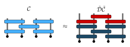
Figure 1: An example of the quantum error mitigation procedure used in this work for the time evolution of the wave function of a spin chain. The ideal second-order Trotter supercircuit $\mathcal{C}$ of depth $M_{\text{trot}}=1$ (light blue) is approximated by applying a denoiser $\tilde{\mathcal{D}}$ of depth $M=1$ (red) to the noisy Trotter supercircuit $\tilde{\mathcal{C}}$ (dark blue). Because the denoiser is applied after fully executing the noisy Trotter supercircuit, it represents an approximate inverse of the global noise channel with a precision tunable by the depth of the denoiser.

Method. — Due to the inevitable coupling of a quantum processor to its environment, every qubit operation is affected by noise. Therefore, the simplest technique to minimize the impact of the resulting noise is to minimize the number of operations when performing a quantum algorithm. In Tepaske et al. (2022) we showed that many-body time evolution operators can be efficiently compressed into brickwall circuits with high fidelity per gate.

In this Letter, we consider the noise explicitly by treating quantum operations as (generally non-unitary) quantum channels, corresponding to completely positive and trace preserving (CPTP) maps Nielsen and Chuang (2011). For example, instead of a noiseless two-qubit gate $G$, which acts on a quantum state $|\rho\rangle\rangle$ in superoperator form as $\mathcal{G}|\rho\rangle\rangle=G\otimes G^{*}|\rho\rangle\rangle$, we get the noisy channel $\tilde{\mathcal{G}}=\mathcal{N}\mathcal{G}$, where the noise channel $\mathcal{N}$ implements the two-qubit noise Aharonov et al. (1998). These channels are used to construct a “supercircuit” $\tilde{\mathcal{C}}=\prod_{i=1}^{N_{\mathcal{G}}}\tilde{\mathcal{G}}_{i}$, consisting of $N_{\mathcal{G}}$ channels, which is affected by multi-qubit accumulated noise. This supercircuit encodes an ensemble of circuits Aharonov et al. (1998). For simplicity, we assume that the noisy channels $\tilde{\mathcal{G}}_{i}$ in each half brickwall layer are lattice inversion and translation invariant, such that we can construct a denoiser with these properties, limiting the number of variational parameters.

The purpose of quantum error mitigation is to modify the ensemble of circuits described by $\tilde{\mathcal{C}}$ in a way that we can use it to obtain the noiseless expectation values. In superoperator language, we do this by following the supercircuit $\tilde{\mathcal{C}}$ with a denoiser supercircuit $\tilde{\mathcal{D}}$, such that $\tilde{\mathcal{D}}\tilde{\mathcal{C}}$ is as close to the noiseless supercircuit $\mathcal{C}=C\otimes C^{*}$ as possible. Here $C$ is the target unitary circuit. Because the noise channel $\mathcal{N}$ is non-unitary, hence making the supercircuit $\tilde{\mathcal{C}}$ non-unitary, we need to use a non-unitary denoiser to retrieve the unitary $\mathcal{C}$.

We illustrate the mitigation procedure in Fig. 1, where a denoiser with one layer is used to mitigate errors for a second-order Trotter supercircuit with one layer. This circuit architecture is commonly used to simulate the time evolution of a quantum many-body system, until some time $t$, with controllable precision Trotter (1959); Suzuki (1976); Paeckel et al. (2019); Tepaske et al. (2022); Ostmeyer (2022); Kargi et al. (2021); Heyl et al. (2019); Childs et al. (2021); Hémery et al. (2019); Mansuroglu et al. (2023); Zhao et al. (2022); Berthusen et al. (2021), and we will use it to benchmark the denoiser. In practice, we cannot directly implement a supercircuit, and so we have to utilize its interpretation as an ensemble of circuits. Essentially, after executing a shot of the noisy circuit we sample the denoiser and apply it. The goal is to construct the denoiser in a way that averaging over many of its samples cancels the accumulated errors and gives us a good approximation of the noiseless expectation values.

It should be noted that our approach requires more gate applications on the quantum processor than with the gate-wise scheme, since there each sample from the mitigation quasiprobability distribution can be absorbed into the original circuit, whereas our approach increases the circuit depth. We take this into account by imposing the same noise on the denoiser. Furthermore, within our scheme, the dimensionality of the quasiprobabilistic mitigating ensemble can be controlled, in contrast to the gate-wise approach where it is equal to the gate count.

To facilitate the stochastic interpretation we parameterize each two-qubit denoiser channel $\mathcal{G}_{i}$ as a sum of CPTP maps, such that we can sample the terms in this sum and execute the sampled gate on the quantum processor. Concretely, we use a trace preserving sum of a unitary and a non-unitary channel. For the unitary part we take a two-qubit unitary channel $\mathcal{U}(\vec{\phi}_{i})=U(\vec{\phi}_{i})\otimes U^{*}(\vec{\phi}_{i})$, with $U(\vec{\phi}_{i})$ a two-qubit unitary gate parameterized by $\vec{\phi}_{i}$. For this we take the two-qubit ZZ rotation $\exp(-i\alpha(\sigma_{z}\otimes\sigma_{z}))$ with angle $\alpha$, which can be obtained from native gates on current hardware Chen et al. (2022), and dress it with four general one-qubit unitaries, only two of which are independent if we want a circuit that is space inversion symmetric around every bond. The resulting gate has 7 real parameters $\vec{\phi}_{i}$.

For the non-unitary part, which is essential because $\tilde{\mathcal{D}}$ has to cancel the non-unitary accumulated noise to obtain the noiseless unitary circuit, we use a general one-qubit measurement followed by conditional preparation channel $\mathcal{M}(\vec{\zeta}_{i})|\rho\rangle\rangle=\sum_{l}K_{l}\otimes K_{l}^{*}|\rho\rangle\rangle$. It has Kraus operators $K_{1}=|\psi_{1}\rangle\langle\,\psi\,|$ and $K_{2}=|\psi_{2}\rangle\langle\,\bar{\psi}\,|$ if we measure in the orthonormal basis $\{|\psi\rangle,|\bar{\psi}\rangle\}$, where $|\bar{\psi}\rangle$ is uniquely defined by $|\psi\rangle$ as they are antipodal points on the Bloch sphere. If the measurement yields $|\psi\rangle$ we prepare $|\psi_{1}\rangle$ and if we measure $|\bar{\psi}\rangle$ we prepare $|\psi_{2}\rangle$. These states can be arbitrary points on the Bloch sphere, i.e. $|\psi_{1}\rangle=V(\vec{\kappa}_{1})|0\rangle$, $|\psi_{2}\rangle=V(\vec{\kappa}_{2})|0\rangle$, $|\psi\rangle=V(\vec{\kappa}_{3})|0\rangle$, with $V$ a general one-qubit unitary and each $\vec{\kappa}_{i}$ a 3-dimensional vector, resulting in a real $9$-dimensional $\vec{\zeta}_{i}$. This yields the two-qubit correlated measurement $\mathcal{M}(\vec{\zeta}_{i})\otimes\mathcal{M}(\vec{\zeta}_{i})$.

With these parts we construct the parameterization

$$\mathcal{G}_{i}=\eta_{0}\mathcal{U}(\vec{\phi}_{i})+\eta_{1}\mathcal{M}(\vec{\zeta}_{i})\otimes\mathcal{M}(\vec{\zeta}_{i}),$$ (1)

with coefficients $\eta_{i}\in\mathbb{R}$ that satisfy $\eta_{0}+\eta_{1}=1$ because $\mathcal{G}_{i}$ is trace preserving. Note that here the tensor product symbol corresponds to combining two one-qubit channels to make a two-qubit channel, whereas in most of the paper it is used to link the column and row indices of a density matrix. We construct the denoiser from the noisy channels $\tilde{\mathcal{G}}_{i}=\mathcal{N}\mathcal{G}_{i}$. With this parameterization one denoiser channel has $17$ independent real parameters, such that a denoiser of depth $M$, i.e. consisting of $M$ brickwall layers, has $34M$ real parameters (we use one unique channel per half brickwall layer). For reference, a general channel has $544M$ parameters.

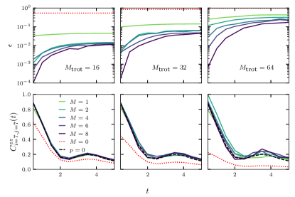
Figure 2: The normalized distance $\epsilon$ between the denoised Trotter supercircuit $\tilde{\mathcal{D}}\tilde{\mathcal{C}}$ and the noiseless Trotter supercircuit $\mathcal{C}$ (top panels), at evolution times $t=0.5,1,...,5$, and the two-point $z$-spin correlator $C^{zz}_{i=L/2,j=L/2}(t)$ of a spin on the middle site at times $0$ and $t$ (bottom panels), for the infinite temperature initial state. We consider denoisers with depths $M=1,2,4,6,8$ and second-order Trotter circuits with depths $M_{\text{trot}}=16,32,64$. In the top panels we use a Heisenberg chain with $L=8$, and in the bottom panels with $L=14$, both with periodic boundary conditions. All gates are affected by two-qubit depolarizing noise with $p=0.01$. The non-denoised results are labelled with $M=0$, and the noiseless values with $p=0$.

To determine the mitigated expectation values we use the full expression

$$\langle\hat{O}\rangle_{p=0}=\langle\langle\mathbb{1}|(\hat{O}\otimes\mathbb{1})\mathcal{C}|\rho_{0}\rangle\rangle\approx\langle\langle\mathbb{1}|(\hat{O}\otimes\mathbb{1})\tilde{\mathcal{D}}\tilde{\mathcal{C}}|\rho_{0}\rangle\rangle,$$ (2)

where $|\rho_{0}\rangle\rangle$ is the initial state and $|\mathbb{1}\rangle\rangle$ is the vectorized identity operator on the full Hilbert space. To evaluate this on a quantum processor, we use the stochastic interpretation of (1) to resample (2). In particular, from each channel (1) we get a unitary with probability $p_{0}=|\eta_{0}|/\gamma$ and a measurement followed by conditional preparation with probability $p_{1}=|\eta_{1}|/\gamma$. Here $\gamma=|\eta_{0}|+|\eta_{1}|$ is the sampling overhead, which characterizes the magnitude of the sign problem from negative $\eta_{i}$ Endo et al. (2018); Temme et al. (2017); Takagi (2021); Piveteau et al. (2022); Guo and Yang (2022b); J. et al. (2021). For quasiprobability distributions, i.e. with $\gamma>1$, every denoiser sample has an extra sign $\text{sgn}(\eta)=\prod_{g=1}^{N_{\mathcal{G}}}\text{sgn}(\eta_{g})$, where $\text{sgn}(\eta_{g})$ is the sign of the sampled coefficient of the $g$th channel. $\gamma=1$ means that all signs are positive. Observables $\langle\hat{O}\rangle_{p=0}$ for the noiseless circuit are then approximated by resampling the observables from the denoiser ensemble Temme et al. (2017)

$$\langle\hat{O}\rangle_{p=0}\approx\gamma\langle\text{sgn}(\eta)\hat{O}\rangle_{p},$$ (3)

where $\gamma=\prod_{g=1}^{N_{\mathcal{G}}}\gamma_{g}$ is the overall sampling overhead, with $\gamma_{g}$ the overhead of the $g$th gate. Clearly, a large $\gamma$ implies a large variance of $\langle\hat{O}\rangle_{p=0}$ for a given number of samples, with accurate estimation requiring the cancellation of large signed terms.

The number of samples required to resolve this cancellation of signs is bounded by Hoeffding’s inequality, which states that a sufficient number of samples to estimate $\langle\hat{O}\rangle_{p=0}$ with error $\delta$ at probability $1-\omega$ is bounded by $(2\gamma^{2}/\delta^{2})\ln(2/\omega)$ Takagi (2021). Since $\gamma$ scales exponentially in $\gamma_{g}$, it is clear that a denoiser with large $M$ and $\gamma\gg 1$ will require many samples.

We observed that decompositions with $\gamma>1$ are crucial for an accurate denoiser. Restricting to $\gamma=1$ leads to large infidelity and no improvement upon increasing the number of terms in (1) or the depth $M$ of the denoiser. Simply put, probabilistic error cancellation of gate noise introduces a sign problem and it is crucial to find optimal parameterizations (1) which minimize $\gamma$ to make the approach scalable. This issue arises in all high performance error mitigation schemes Temme et al. (2017); Takagi (2021); J. et al. (2021); van den Berg et al. (2022), because the inverse of a physical noise channel is unphysical and cannot be represented as a positive sum over CPTP maps. This is clearly visible in the spectra of the denoiser, which lies outside the unit circle (cf. Fig. 4). This makes the tunability of the number of gates in each denoiser sample a crucial ingredient, which allows control over the sign problem, because we can freely choose the $\eta_{i}$ in (1).

For the parametrization (1) of denoiser channels, we try to find a set of parameters for error mitigation by minimizing the normalized Frobenius distance between the noiseless and denoised supercircuits Tepaske et al. (2022)

$$\epsilon=||\mathcal{C}-\tilde{\mathcal{D}}\tilde{\mathcal{C}}||^{2}_{F}/4^{L},$$ (4)

which bounds the distance of output density matrices and becomes zero for perfect denoising.

We carry out the minimization of $\epsilon$ on a classical processor, using gradient descent with the differential programming algorithm from Tepaske et al. (2022). Instead of explicitly calculating the accumulated global noise channel and subsequently inverting it, we approximate the noiseless supercircuit $\mathcal{C}$ with the denoised supercircuit $\tilde{\mathcal{D}}\tilde{\mathcal{C}}$, effectively yielding a circuit representation $\mathcal{D}$ of the inverse noise channel.

Results. — To benchmark the denoiser we apply it to the second-order Trotter circuits of the spin-$1/2$ Heisenberg chain with periodic boundary conditions (PBC)

$$H=\sum_{i=1}^{L}\left(\sigma^{i}_{1}\sigma^{i+1}_{1}+\sigma^{i}_{2}\sigma^{i+1}_{2}+\sigma^{i}_{3}\sigma^{i+1}_{3}\right),$$ (5)

where $\sigma^{i}_{\alpha}=(\mathbb{1}^{i},\sigma^{i}_{x},\sigma^{i}_{y},\sigma^{i}_{z})$ is the Pauli algebra acting on the local Hilbert space of site $i$. A second-order Trotter circuit for evolution time $t$ with depth $M_{\text{trot}}$ consists of $M_{\text{trot}}-1$ half brickwall layers with time step $t/M_{\text{trot}}$ and two layers with half time step Tepaske et al. (2022); Paeckel et al. (2019). We consider circuits that are affected by uniform depolarizing noise with probability $p$ for simplicity, but our approach can be used for any non-Clifford noise. The two-qubit noise channel is

$$\mathcal{N}=\left(1-\frac{16p}{15}\right)\mathbb{1}+\frac{p}{15}\bigotimes_{j=i}^{i+1}\left(\sum_{\alpha=0}^{3}\sigma^{j}_{\alpha}\otimes\sigma^{j*}_{\alpha}\right),$$ (6)

which acts on neighboring qubits $i$ and $i+1$ and is applied to each Trotter and denoiser gate, and $p=0.01$ unless stated otherwise. We study circuits with depths $M_{\text{trot}}=16,32,64$ for evolution times $t=0.5,1,...,5$, and denoisers $\tilde{\mathcal{D}}$ with depths $M=1,2,4,6,8$.

In the top panels of Fig. 2 we show $\epsilon$ (4) for a chain of size $L=8$ as a function of time $t$. Here it can be seen that even for $M_{\text{trot}}=32$ a denoiser with $M=1$ already improves $\epsilon$ by roughly an order of magnitude at all considered $t$. Depending on $M_{\text{trot}}$ and $t$, further increasing $M$ lowers $\epsilon$, with the biggest improvements occurring for high precision Trotter circuits with large depth $M_{\text{trot}}=64$ and short time $t=0.5$, where the Trotter gates are closer to the identity than in the other cases. At the other extreme, for $M_{\text{trot}}=16$ the improvements are relatively small upon increasing $M>2$. In all cases the denoiser works better at early times than at late times, again indicating that it is easier to denoise Trotter gates that are relatively close to the identity.

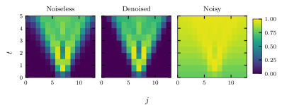
Figure 3: The out-of-time-ordered correlator $C^{\text{otoc}}_{i=L/2,j}(t)$ as a function of the operator position $j$ and time $t$, for the infinite temperature initial state, for a denoised second-order Trotter supercircuit with Trotter depth $M_{\text{trot}}=32$ and denoiser depth $M=2$. We consider evolution times $t=0.5,1,...,5$, for the periodic $L=14$ Heisenberg chain that is affected by two-qubit depolarizing noise with $p=0.01$.

To probe the accuracy of the denoiser on quantities that do not enter the optimization, as a first test we consider the two-point correlator between spins at different times Dupont and Moore (2020)

$$C^{zz}_{ij}(t)=\langle\langle\mathbb{1}|(\sigma^{z}_{i}\otimes\mathbb{1})\tilde{\mathcal{D}}\tilde{\mathcal{C}}(t)(\sigma^{z}_{j}\otimes\mathbb{1})|\mathbb{1}\rangle\rangle/2^{L},$$ (7)

where we have chosen the infinite temperature initial state, and $\tilde{\mathcal{C}}(t)$ is the Trotter supercircuit for time $t$. In the bottom panels of Fig. 2 we show $C^{zz}_{i=L/2,j=L/2}(t)$ for the supercircuits from the upper panels, now for a $L=14$ chain. Here we see that at $M_{\text{trot}}=16$ we can retrieve the noiseless values already with $M=1$, but that increasing $M_{\text{trot}}$ makes this more difficult. At $M_{\text{trot}}=64$ we see larger deviations, and improvement upon increasing $M$ is less stable, but nonetheless we are able to mitigate errors to a large extent.

As a further test, we compute the out-of-time-ordered correlator (OTOC) Zhang et al. (2019); Tepaske et al. (2022); Hémery et al. (2019); Luitz and Bar Lev (2017); Maldacena et al. (2016); Larkin and Ovchinnikov (1969)

$$C^{\text{otoc}}_{ij}(t)=\textrm{Re}\langle\langle\mathbb{1}|(\sigma^{z\dagger}_{j}\otimes\mathbb{1})\tilde{\mathcal{D}}\tilde{\mathcal{C}}(-t)\\ (\sigma_{i}^{z}\otimes\sigma_{i}^{z*})\tilde{\mathcal{D}}\tilde{\mathcal{C}}(t)(\sigma^{z}_{j}\otimes\mathbb{1})|\mathbb{1}\rangle\rangle/2^{L}.$$ (8)

In Fig. 3 we show the results for $i=L/2$, for a Trotter circuit with depth $M_{\text{trot}}=32$ and a denoiser with depth $M=2$. Here we see that a denoiser with $M\ll M_{\text{trot}}$ is able to recover the light-cone of correlations, which are otherwise buried by the noise. In the Supplementary Material we consider how the denoiser performs at different noise levels $p$, and how the denoised supercircuits perform under stacking. There we also calculate domain wall magnetization dynamics, and show the distribution of the optimized denoiser parameters and the sampling overhead associated to the denoiser as a whole.

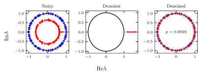
Figure 4: The complex eigenvalues $\lambda$ of the noisy second-order Trotter supercircuit with $M_{\text{trot}}=16$ at time $t=1$ (left), the corresponding optimized denoiser with $M=4$ (center), and the denoised Trotter supercircuit (right). The Trotter circuit is for a $L=6$ Heisenberg model with PBC, and all two-qubit channels are affected by depolarizing noise with $p=0.0046$. The unit circle, on which unitary eigenvalues must lie, is shown in black, and the noiseless eigenvalues are shown as blue bars. It is evident that the denoiser recovers all the noiseless eigenvalues from the noisy circuit.

In Fig. 4 we show the eigenvalues of the noisy supercircuits for a noisy second-order Trotter supercircuit with $M_{\text{trot}}=16$ at $t=1$ (left), the corresponding optimized denoiser with $M=4$ (center), and the denoised supercircuit (right). The eigenvalues $\lambda$ of a unitary supercircuit lie on the unit circle, and in the presence of dissipation they are pushed to the center. We see that the spectrum of the denoiser lies outside the unit circle, making it an unphysical channel which cures the effect of the noise on the circuit, such that the spectrum of the denoised circuit is pushed back to the unit circle. The noiseless eigenvalues are shown as blue bars, making it clear that the denoiser is able to recover the noiseless eigenvalues from the noisy circuit. In the Supplementary Material we show the spectra for a $p=0.036$ denoiser, where we observe a clustering of eigenvalues reminiscent of Refs. Wang et al. (2020); Li et al. (2022); Sommer et al. (2021). There we also investigate the channel entropy of the various supercircuits Zhou and Luitz (2017); Roga et al. (2013).

Conclusion. — We have introduced a probabilistic error cancellation scheme, where a classically determined denoiser mitigates the accumulated noise of a (generally non-Clifford) local noise channel. The required number of mitigation gates, i.e. the dimensionality of the corresponding quasiprobability distribution, is tunable and the parameterization of the corresponding channels provides control over the sign problem that is inherent to probabilistic error cancellation. We have shown that a denoiser with one layer can already significantly mitigate errors for second-order Trotter circuits with up to $64$ layers.

This effectiveness of low-depth compressed circuits for denoising, in contrast with the noiseless time evolution operator compression from Tepaske et al. (2022), can be understood from the non-unitarity of the denoiser channels. In particular, measurements can have non-local effects, since the measurement of a single qubit can reduce some highly entangled state (e.g. a GHZ state) to a product state, whereas in unitary circuits the spreading of correlations forms a light-cone.

To optimize a denoiser with convenience at $L>8$, the optimization can be formulated in terms of matrix product operators Tepaske et al. (2022); Guo and Yang (2022a) or channels Filippov et al. (2022), which is convenient because the circuit calculations leading to the normalized distance $\epsilon$ and its gradient are easily formulated in terms of tensor contractions and singular value decompositions Tepaske et al. (2022); Noh et al. (2020). This provides one route to a practical denoiser, which is relevant because the targeted noiseless circuit and the accompanying noisy variant in (4) need to be simulated classically, confining the optimization procedure to limited system sizes with an exact treatment or limited entanglement with tensor networks. Nonetheless, we can use e.g. matrix product operators to calculate (4) for some relatively small $t$, such that the noiseless and denoised supercircuits in (4) have relatively small entanglement, and then stack the final denoised supercircuit on a quantum processor to generate classically intractable states. Analogously, we can optimize the channels exactly at some classically tractable size and then execute them on a quantum processor with larger size. Both approaches are limited by the light-cone of many-body correlations, as visualized in Fig. 3, because finite-size effects appear when the light-cone width becomes comparable with system size.

I Supplementary material

I.1 Denoiser performance at various noise levels

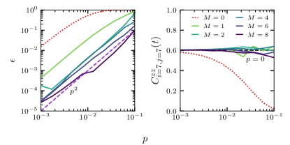
Figure 5: The normalized distance $\epsilon$ (left) and $z$ spin correlator $C^{zz}_{i=L/2,j=L/2}$ (right), for a second-order Trotter supercircuit of depth $M_{\text{trot}}=16$ for time $t=1$, affected by various two-qubit depolarizing errors $p$. We compare the values obtained with and without a denoiser, i.e. $M>0$ and $M=0$, to the noiseless values ($p=0$). The denoiser is affected by the same noise as the Trotter circuit. We consider denoisers with depths $M=1,2,4,6,8$, and we use a $L=8$ Heisenberg chain with PBC for the normalized distance, while for the correlator we use $L=14$.

To probe how the denoiser performs at different noise strengths $p$, we take a second-order Trotter supercircuit of depth $M_{\text{trot}}=16$ for the time evolution of the wave function to time $t=1$, and optimize the denoiser at various noise strengths in the interval $p\in\left[10^{-3},10^{-1}\right]$. In Fig. 5 we show the normalized distance (left panel) and the $z$ spin correlator (right), for denoiser depths $M=1,2,4,6,8$. For comparison, we show the results for the noisy limit, i.e. without a denoiser ($M=0$, red dashed), and for the exact limit without noise ($p=0$, black dashed).

The error of the entire circuit $\epsilon$ improves with denoiser depth $M$ for the full range of $p$, and depends roughly quadratically on $p$. This is illustrated with the purple dashed line in the left panel of Fig. 5. It is interesting to observe that even for larger noise strength $p$, the local observable $C^{zz}$ improves significantly even with denoisers of depth $M=1$. For large noise strengths, we generally see that the optimization of the denoiser becomes difficult, leading to nonmonotonic behavior as a function of $p$, presumably because we do not find the global optimum of the denoiser.

I.2 Supercircuit spectra

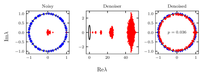
Figure 6: The complex eigenvalues $\lambda$ of the noisy second-order Trotter supercircuit with $M_{\text{trot}}=16$ at time $t=1$ (left), the corresponding optimized denoiser with $M=4$ (center), and the denoised Trotter supercircuit (right). The Trotter circuit is for a $L=6$ Heisenberg model with PBC, and all two-qubit channels are affected by depolarizing noise with $p=0.036$. The unit circle, on which unitary eigenvalues must lie, is shown in black, and the noiseless eigenvalues are shown as blue bars. It is clear that the denoiser recovers with high accuracy the noiseless eigenvalues from the noisy circuit.

It is interesting to analyze the spectra of the supercircuits considered in this work. As mentioned in the main text, the spectrum of the ideal, unitary supercircuit $\mathcal{C}$ lies on the unit circle. The comparison to this case is therefore instructive. In the main text, we showed an example of the spectra in Fig. 4 for moderate noise strength. Here, we show additional data for stronger noise $p=0.036$ in Fig. 6 for a denoiser with $M=4$ layers, optimized to mitigate errors for a second-order Trotter supercircuit with $M_{\text{trot}}=16$ layers at time $t=1$.

The eigenvalues $\lambda$ of the noisy supercircuit $\mathcal{\tilde{C}}$ are clustered close to zero, far away from the unit circle (except for $\lambda=1$), showing that the circuit is strongly affected by the noise. To mitigate the impact of the noise, the denoiser consequently has to renormalize the spectrum strongly. If it accurately represents the inverse of the global noise channel, its spectrum has to lie far outside the unit circle, which is the case. Interestingly, we observe a clustering of eigenvalues which is reminiscent to the spectra found in Wang et al. (2020); Sommer et al. (2021); Li et al. (2022). By comparison to these works, we suspect that this is due to the local nature of the denoiser, and warrants further investigation.

The right panel of Fig. 6 shows the result of the denoiser, pushing the eigenvalues back to the unit circle, nearly with the exact same distribution along the circle as the noiseless eigenvalues (blue bars). Due to the strong noise, this is not achieved perfectly, and it is clear that this cannot work in principle if the global noise channel has a zero eigenvalue.

I.3 Supercircuit entropies

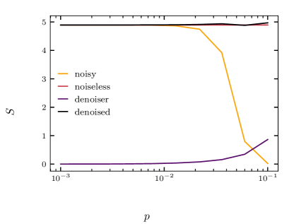
Figure 7: The half-chain channel entanglement entropy $S$ at different two-qubit depolarizing noise strengths $p$, for a second-order Trotter supercircuit with $M_{\text{trot}}=16$ and $t=2$, for a $M=4$ denoiser. The Trotter circuit is for a Heisenberg model with PBC of size $L=6$. The different curves correspond to the different supercircuits, i.e. the noisy supercircuit, the denoiser, the corresponding denoised supercircuit, and the noiseless variant.

The complexity of an operator can be quantified by its operator entanglement entropy Zhou and Luitz (2017). Here we calculate the half-chain channel entanglement entropy $S$ Roga et al. (2013) of the noiseless $\mathcal{C}$, noisy $\tilde{\mathcal{C}}$, denoiser $\tilde{\mathcal{D}}$, and denoised $\tilde{\mathcal{D}}\tilde{\mathcal{C}}$ supercircuits. We define $S$ as the entanglement entropy of the state that is related to a supercircuit $\mathcal{C}$ via the Choi-Jamiołkowski isomorphism, i.e. $\psi_{\mathcal{C}}=\chi_{\mathcal{C}}/N$, where the process matrix $\chi^{ab,cd}_{\mathcal{C}}=\mathcal{C}^{ac,bd}$ is simply a reshaped supercircuit and $N$ ensures normalization. Then we have $S=-\mathrm{Tr}\left[\psi_{\mathcal{C}}\ln\psi_{\mathcal{C}}\right]$. This entropy measure is a particular instance of the “exchange entropy”, which characterizes the information exchange between a quantum system and its environment Roga et al. (2013).

In Fig. 7 we plot the various $S$ for a second-order Trotter circuit with $M_{\text{trot}}=16$ at $t=2$, for a denoiser with $M=4$, both affected by two-qubit depolarizing noise with $p\in[10^{-3},10^{-1}]$. The Trotter circuit is for a Heisenberg model with $L=6$ and PBC. We see that at large $p$, the noise destroys entanglement in the noisy supercircuit, and that the denoiser $S$ increases to correct for this, such that the denoised supercircuit recovers the noiseless $S$.

I.4 Stacking denoised supercircuits

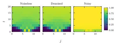
Figure 8: The out-of-time-ordered correlator $C^{\text{otoc}}_{i=L/2,j}(t)$ as a function of the operator position $j$ and stacked time $t$, for the infinite temperature initial state, for a denoised second-order Trotter supercircuit with Trotter depth $M_{\text{trot}}=32$ and denoiser depth $M=2$. It is optimized at $t=2$ and stacked up to ten times. The calculations are for the periodic $L=14$ Heisenberg chain that is affected by two-qubit depolarization with $p=0.01$. The denoiser is affected by the same noise.

Figure 9: The two-point $z$-spin correlator $C^{zz}_{i=L/2,j=L/2}(t)$ of a spin on the middle site at times $0$ and $t$, for the infinite temperature initial state, for denoised second-order Trotter supercircuits that are optimized at evolution time $t=1$ and then stacked up to twenty times. We use Trotter depths $M_{\text{trot}}=8,16,32,64$ and denoiser depths $M=1,2,4,6,8$. The calculations were performed for a periodic Heisenberg model with $L=14$ and PBC, affected by two-qubit depolarizing noise with strength $p=0.01$, which also affects the denoiser. The non-denoised results are labelled with $M=0$, and the noiseless results with $p=0$. The panels are arranged as $M_{\text{trot}}=8,16,32,64$ for top left, top right, bottom left, bottom right, respectively.

Here we investigate how denoised supercircuits perform upon repeated application. We optimize the denoiser for a Trotter supercircuit for a fixed evolution time $t$. Then, to reach later times, we stack the denoised supercircuit $n$ times to approximate the evolution up to time $nt$:

$$\mathcal{C}(nt)\approx\left(\tilde{\mathcal{D}}(t)\tilde{\mathcal{C}}(t)\right)^{n}$$ (9)

In Fig. 9 we stack a denoised $t=1$ supercircuit up to $n=20$ times and calculate the correlation function, defined in the main text, for the middle site. We consider Trotter depths $M_{\text{trot}}=8,16,32,64$ and denoiser depths $M=1,2,4,6,8$, for a $L=14$ Heisenberg chain with $p=0.01$ depolarizing two-qubit noise. The noisy results correspond to $M=0$ and the noiseless results to $p=0$. In Fig. 8 we calculate the OTOC, defined in the main text, with stacked time evolution for a denoised $t=2$ supercircuit with $M_{\text{trot}}=32$ and $M=2$, stacked up to ten times. We see that the stacked supercircuit performs very well, and the additional precision obtained by using deep denoisers ($M=8$) pays off for long evolution times, where we see convergence to the exact result (black dashed lines in Fig. 9) as a function of $M$.

I.5 Distribution of optimized ZZ channels

The costliest and most noise-susceptible operation is the two-qubit $ZZ$ rotation with angle $\alpha$, which is the foundation of the unitary piece in our channel parameterization, defined in the main text. For completeness, we here present the $\alpha$ angles of the optimized denoisers. The results are shown in Fig. 10, which contains histograms for the channel count $N_{\mathcal{G}}$ versus $\alpha$. The histograms are stacked, with the lightest color corresponding to the angles of the denoiser at $t=0.5$ and the darkest at $t=5$. The top four panels are for a denoiser with $M=2$ and the bottom four with $M=8$. We consider $M_{\text{trot}}=8,16,32,64$. We see that in both cases the distribution widens upon increasing $M_{\text{trot}}$, indicating that the unitary channels start deviating more from the identity. Moreover, while the $M=2$ denoisers in all cases except $M_{\text{trot}}=64$ have ZZ contributions close to the identity, this is clearly not the case for $M=8$.

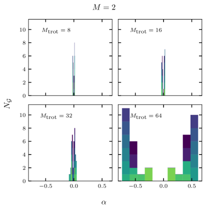
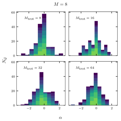
Figure 10: The distribution of the ZZ angle $\alpha$ of $M=2$ denoisers (top panels) and $M=8$ denoisers (bottom panels), with the lightest color corresponding to the denoiser for the Trotter supercircuit with $t=0.5$, and the darkest color with $t=5$. As usual, we consider the Heisenberg model on a periodic chain, and second-order Trotter supercircuits with depths $M_{\text{trot}}=8,16,32,64$, which together with the denoiser is affected by a two-qubit depolarizing noise with $p=0.01$. The panels are arranged as $M_{\text{trot}}=8,16,32,64$ for top left, top right, bottom left, bottom right, respectively.

I.6 Sampling overhead of optimized denoisers

For simplicity, we did not focus on obtaining denoisers with the smallest sampling overhead $\gamma$, which is required to minimize the sign problem and hence ease the sampling of mitigated quantities. Instead, we let the optimization freely choose the $\eta_{i}$ in the denoiser parameterization, as defined in the main text. In Fig. 11 we show the sampling overhead of the denoisers from Fig. 2 of the main text. We see that for $M=1$ and $M=2$ the sampling overhead is relatively small and uniform across the different $t$, whereas for $M>2$ the optimization sometimes yields a denoiser with large $\gamma$ and other times with small $\gamma$. This could be related to the difference in $\alpha$ distributions from Fig. 10. The large fluctuations of $\gamma$ appears to stem from the difficulty in finding optimal deep denoisers, and our optimization procedure likely only finds a local minimum in these cases.

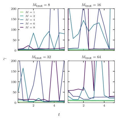
Figure 11: The sampling overhead $\gamma$ of the optimized denoisers from Fig. 2 of the main text, with denoiser depths $M=1,2,4,6,8$ and Trotter depths $M_{\text{trot}}=8,16,32,64$ at times $t=0.5,1,...,5$, for the Heisenberg model on a chain with PBC affected by two-qubit depolarizing noise with $p=0.01$. The panels are arranged as $M_{\text{trot}}=8,16,32,64$ for top left, top right, bottom left, bottom right, respectively.

I.7 Domain wall magnetization

As another test of the denoiser performance we evolve the periodic $z$-spin domain wall $|\text{dw}\rangle=\bigotimes_{i=1}^{L/2}|1\rangle\otimes\bigotimes_{i=L/2}^{L}|0\rangle$ and consider the domain wall magnetization

$$Z^{\text{dw}}(t)=\sum_{i=1}^{L}(-1)^{\lfloor 2i/L\rfloor}\langle\langle\mathbb{1}|(\sigma^{z}_{i}\otimes\mathbb{1})\tilde{\mathcal{D}}\tilde{\mathcal{C}}(t)|\text{dw}\rangle|\text{dw}^{*}\rangle.$$ (10)

Here $\tilde{\mathcal{C}}(t)$ is the Trotter supercircuit for time $t$. In Fig. 12 we show $Z^{\text{dw}}$ for the circuits from Fig. 2 of the main text, calculated for a $L=14$ chain. As in our other tests, we see that at $M_{\text{trot}}=8$ we can recover the noiseless values already with $M=1$, and that increasing $M_{\text{trot}}$ makes this more difficult. At $M_{\text{trot}}=64$ we see larger deviations, and improvement upon increasing $M$ is less stable, but nevertheless we are able to mitigate errors to a large extent.

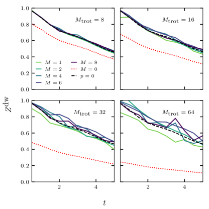
Figure 12: The domain wall magnetization $Z^{\text{dw}}$ after evolving a periodic density wall $|\text{dw}\rangle|\text{dw}^{*}\rangle$ with the denoised second-order Trotter supercircuits $\tilde{\mathcal{D}}\tilde{\mathcal{C}}$ from Fig. 2 of the main text. These supercircuits have various Trotter depths $M_{\text{trot}}=8,16,32,64$, denoiser depths $M=1,2,4,6,8$, and evolution times $t=0.5,1,...,5$, for the periodic $L=14$ Heisenberg chain that is affected by two-qubit depolarizing noise of strength $p=0.01$. The denoiser is affected by the same noise. The non-denoised results are labelled with $M=0$ and the noiseless results with $p=0$. The panels are arranged as $M_{\text{trot}}=8,16,32,64$ for top left, top right, bottom left, bottom right, respectively. We see that the denoiser allows us to recover the noiseless behavior.

References

- Kitaev (1995) A. Y. Kitaev, “Quantum measurements and the abelian stabilizer problem,” (1995), arXiv:quant-ph/9511026 .
- Shor (1997) P. W. Shor, “Polynomial-time algorithms for prime factorization and discrete logarithms on a quantum computer,” SIAM Journal on Computing 26, 1484–1509 (1997).
- Ebadi et al. (2022) S. Ebadi, A. Keesling, M. Cain, T. T. Wang, H. Levine, D. Bluvstein, G. Semeghini, and et al., “Quantum optimization of maximum independent set using rydberg atom arrays,” (2022), arXiv:2202.09372 .
- Arute et al. (2019) F. Arute, K. Arya, R. Babbush, D. Bacon, J. C. Bardin, R. Barends, R. Biswas, S. Boixo, and et al., “Quantum supremacy using a programmable superconducting processor,” Nature 574, 505–510 (2019).
- Feynman (1982) R. P. Feynman, “Simulating physics with computers,” International Journal of Theoretical Physics 21, 467–488 (1982).
- Lloyd (1996) S. Lloyd, “Universal Quantum Simulators,” Science 273, 1073 (1996).
- B. et al. (2021) Stefano B., Filippo V., and Giuseppe C., “An efficient quantum algorithm for the time evolution of parameterized circuits,” Quantum 5, 512 (2021).
- Bañuls et al. (2020) M. C. Bañuls, R. Blatt, J. Catani, A. Celi, J. I. Cirac, M. Dalmonte, L. Fallani, and et al., “Simulating lattice gauge theories within quantum technologies,” The European Physical Journal D 74, 165 (2020).
- Scholl et al. (2021) P. Scholl, M. Schuler, H. J. Williams, A. A. Eberharter, D. Barredo, K.-N. Schymik, V. Lienhard, and et al., “Quantum simulation of 2d antiferromagnets with hundreds of rydberg atoms,” Nature 595, 233–238 (2021).
- Preskill (2018) J. Preskill, “Quantum Computing in the NISQ era and beyond,” Quantum 2, 79 (2018).
- Calderbank and Shor (1996) A. R. Calderbank and P. W. Shor, “Good quantum error-correcting codes exist,” Phys. Rev. A 54, 1098–1105 (1996).
- Shor (1995) P. W. Shor, “Scheme for reducing decoherence in quantum computer memory,” Phys. Rev. A 52, R2493–R2496 (1995).
- Temme et al. (2017) K. Temme, S. Bravyi, and J. M. Gambetta, “Error mitigation for short-depth quantum circuits,” Phys. Rev. Lett. 119, 180509 (2017).
- Endo et al. (2018) S. Endo, S. C. Benjamin, and Y. Li, “Practical quantum error mitigation for near-future applications,” Phys. Rev. X 8, 031027 (2018).
- Vovrosh et al. (2021) J. Vovrosh, K. E. Khosla, S. Greenaway, C. Self, M. S. Kim, and J. Knolle, “Simple mitigation of global depolarizing errors in quantum simulations,” Phys. Rev. E 104, 035309 (2021).
- Filippov et al. (2022) S. Filippov, B. Sokolov, M. A. C. Rossi, J. Malmi, E.-M. Borrelli, D. Cavalcanti, S. Maniscalco, and G. García-Pérez, “Matrix product channel: Variationally optimized quantum tensor network to mitigate noise and reduce errors for the variational quantum eigensolver,” (2022), arXiv:2212.10225 .
- Cao et al. (2021) N. Cao, J. Lin, D. Kribs, Y.-T. Poon, B. Zeng, and R. Laflamme, “Nisq: Error correction, mitigation, and noise simulation,” (2021), arXiv:2111.02345 .
- Piveteau et al. (2022) C. Piveteau, D. Sutter, and S. Woerner, “Quasiprobability decompositions with reduced sampling overhead,” npj Quantum Information 8, 12 (2022).
- Gutiérrez et al. (2016) M. Gutiérrez, C. Smith, L. Lulushi, S. Janardan, and K. R. Brown, “Errors and pseudothresholds for incoherent and coherent noise,” Phys. Rev. A 94, 042338 (2016).
- J. et al. (2021) Jiaqing J., Kun W., and Xin W., “Physical implementability of linear maps and its application in error mitigation,” Quantum 5, 600 (2021).
- Magesan et al. (2013) E. Magesan, D. Puzzuoli, C. E. Granade, and D. G. Cory, “Modeling quantum noise for efficient testing of fault-tolerant circuits,” Phys. Rev. A 87, 012324 (2013).
- Cai et al. (2022) Z. Cai, R. Babbush, S. C. Benjamin, S. Endo, W. J. Huggins, Y. Li, J. R. McClean, and T. E. O’Brien, “Quantum error mitigation,” (2022), arXiv:2210.00921 .
- Ferracin et al. (2022) Samuele Ferracin, Akel Hashim, Jean-Loup Ville, Ravi Naik, Arnaud Carignan-Dugas, Hammam Qassim, Alexis Morvan, David I. Santiago, Irfan Siddiqi, and Joel J. Wallman, “Efficiently improving the performance of noisy quantum computers,” (2022), arXiv:2201.10672 .
- van den Berg et al. (2022) E. van den Berg, Z. K. Minev, A. Kandala, and K. Temme, “Probabilistic error cancellation with sparse pauli-lindblad models on noisy quantum processors,” (2022), arXiv:2201.09866 .
- McDonough et al. (2022) Benjamin McDonough, Andrea Mari, Nathan Shammah, Nathaniel T. Stemen, Misty Wahl, William J. Zeng, and Peter P. Orth, “Automated quantum error mitigation based on probabilistic error reduction,” in 2022 IEEE/ACM Third International Workshop on Quantum Computing Software (QCS) (IEEE, 2022).
- Guo and Yang (2022a) Y. Guo and S. Yang, “Quantum error mitigation via matrix product operators,” PRX Quantum 3, 040313 (2022a).
- Flannigan et al. (2022) S. Flannigan, N. Pearson, G. H. Low, A. Buyskikh, I. Bloch, P. Zoller, M. Troyer, and A. J. Daley, “Propagation of errors and quantitative quantum simulation with quantum advantage,” (2022), arXiv:2204.13644 .
- Poggi et al. (2020) P. M. Poggi, N. K. Lysne, K. W. Kuper, I. H. Deutsch, and P. S. Jessen, “Quantifying the sensitivity to errors in analog quantum simulation,” PRX Quantum 1, 020308 (2020).
- Tepaske et al. (2022) M. S. J. Tepaske, D. Hahn, and D. J. Luitz, “Optimal compression of quantum many-body time evolution operators into brickwall circuits,” (2022), arXiv:2205.03445 .
- Nielsen and Chuang (2011) M. A. Nielsen and I. L. Chuang, Quantum Computation and Quantum Information: 10th Anniversary Edition (Cambridge University Press, 2011).
- Aharonov et al. (1998) D. Aharonov, A. Kitaev, and N. Nisan, “Quantum circuits with mixed states,” (1998), arXiv:quant-ph/9806029 .
- Trotter (1959) H. F Trotter, “On the product of semi-groups of operators,” Proceedings of the American Mathematical Society 10, 545–551 (1959).
- Suzuki (1976) M. Suzuki, “Generalized Trotter’s formula and systematic approximants of exponential operators and inner derivations with applications to many-body problems,” Communications in Mathematical Physics 51, 183 – 190 (1976).
- Paeckel et al. (2019) S. Paeckel, T. Köhler, A. Swoboda, S. R. Manmana, U. Schollwöck, and C. Hubig, “Time-evolution methods for matrix-product states,” Annals of Physics 411, 167998 (2019).
- Ostmeyer (2022) J. Ostmeyer, “Optimised trotter decompositions for classical and quantum computing,” (2022), arXiv:2211.02691 .
- Kargi et al. (2021) C. Kargi, J. P. Dehollain, F. Henriques, L. M. Sieberer, T. Olsacher, P. Hauke, M. Heyl, P. Zoller, and N. K. Langford, “Quantum chaos and universal trotterisation behaviours in digital quantum simulations,” (2021), arXiv:2110.11113 .
- Heyl et al. (2019) M. Heyl, P. Hauke, and P. Zoller, “Quantum localization bounds trotter errors in digital quantum simulation,” Science Advances 5, eaau8342 (2019).
- Childs et al. (2021) A. M. Childs, Y. Su, M. C. Tran, N. Wiebe, and S. Zhu, “Theory of trotter error with commutator scaling,” Physical Review X 11, 011020 (2021).
- Hémery et al. (2019) K. Hémery, F. Pollmann, and D. J. Luitz, “Matrix product states approaches to operator spreading in ergodic quantum systems,” Phys. Rev. B 100, 104303 (2019).
- Mansuroglu et al. (2023) R. Mansuroglu, T. Eckstein, L. Nützel, S. A Wilkinson, and M. J Hartmann, “Variational hamiltonian simulation for translational invariant systems via classical pre-processing,” Quantum Science and Technology 8, 025006 (2023).
- Zhao et al. (2022) H. Zhao, M. Bukov, M. Heyl, and R. Moessner, “Making trotterization adaptive for nisq devices and beyond,” (2022), arXiv:2209.12653 .
- Berthusen et al. (2021) N. F. Berthusen, T. V. Trevisan, T. Iadecola, and P. P. Orth, “Quantum dynamics simulations beyond the coherence time on nisq hardware by variational trotter compression,” (2021), arXiv:2112.12654 .
- Chen et al. (2022) I. Chen, B. Burdick, Y. Yao, P. P. Orth, and T. Iadecola, “Error-mitigated simulation of quantum many-body scars on quantum computers with pulse-level control,” Phys. Rev. Res. 4, 043027 (2022).
- Takagi (2021) R. Takagi, “Optimal resource cost for error mitigation,” Phys. Rev. Res. 3, 033178 (2021).
- Guo and Yang (2022b) Y. Guo and S. Yang, “Noise effects on purity and quantum entanglement in terms of physical implementability,” (2022b), arXiv:2207.01403 .
- Dupont and Moore (2020) M. Dupont and J. E. Moore, “Universal spin dynamics in infinite-temperature one-dimensional quantum magnets,” Phys. Rev. B 101, 121106 (2020).
- Zhang et al. (2019) Y.-L. Zhang, Y. Huang, and X. Chen, “Information scrambling in chaotic systems with dissipation,” Phys. Rev. B 99, 014303 (2019).
- Luitz and Bar Lev (2017) D. J. Luitz and Y. Bar Lev, “Information propagation in isolated quantum systems,” Phys. Rev. B 96, 020406 (2017).
- Maldacena et al. (2016) J. Maldacena, S. H. Shenker, and D. Stanford, “A bound on chaos,” Journal of High Energy Physics 2016, 106 (2016).
- Larkin and Ovchinnikov (1969) A. I. Larkin and Yu. N. Ovchinnikov, “Quasiclassical Method in the Theory of Superconductivity,” Soviet Journal of Experimental and Theoretical Physics 28, 1200 (1969).
- Wang et al. (2020) K. Wang, F. Piazza, and D. J. Luitz, “Hierarchy of relaxation timescales in local random liouvillians,” Phys. Rev. Lett. 124, 100604 (2020).
- Li et al. (2022) J. L. Li, D. C. Rose, J. P. Garrahan, and D. J. Luitz, “Random matrix theory for quantum and classical metastability in local liouvillians,” Phys. Rev. B 105, L180201 (2022).
- Sommer et al. (2021) O. E. Sommer, F. Piazza, and D. J. Luitz, “Many-body hierarchy of dissipative timescales in a quantum computer,” Physical Review Research 3, 023190 (2021).
- Zhou and Luitz (2017) T. Zhou and D. J. Luitz, “Operator entanglement entropy of the time evolution operator in chaotic systems,” Physical Review B 95, 094206 (2017).
- Roga et al. (2013) W. Roga, Z. Puchała, Ł. Rudnicki, and K. Žyczkowski, “Entropic trade-off relations for quantum operations,” Phys. Rev. A 87, 032308 (2013).
- Noh et al. (2020) K Noh, L Jiang, and B Fefferman, “Efficient classical simulation of noisy random quantum circuits in one dimension,” Quantum 4, 318 (2020).