Distillation of encoder-decoder transformers for sequence labelling

Abstract

Driven by encouraging results on a wide range of tasks, the field of NLP is experiencing an accelerated race to develop bigger language models. This race for bigger models has also underscored the need to continue the pursuit of practical distillation approaches that can leverage the knowledge acquired by these big models in a compute-efficient manner. Having this goal in mind, we build on recent work to propose a hallucination-free framework for sequence tagging that is especially suited for distillation. We show empirical results of new state-of-the-art performance across multiple sequence labelling datasets and validate the usefulness of this framework for distilling a large model in a few-shot learning scenario.

Distillation of encoder-decoder transformers for sequence labelling

Marco Farina ¹      Duccio Pappadopulo ¹      Anant Gupta¹ Leslie Huang¹      Ozan İrsoy¹     Thamar Solorio ^{1,2 1}Bloomberg       ²Department of Computer Science, University of Houston {mfarina19, dpappadopulo, agupta968, lhuang328, oirsoy}@bloomberg.net thamar.solorio@gmail.com

1 Introduction

Sequence labelling (SL) can be defined as the task of assigning a label to a span in the input text. Some examples of SL tasks are: i) named entity recognition (NER), where these labelled spans refer to people, places, or organizations, and ii) slot-filling, where these spans or slots of interest refer to attributes relevant to complete a user command, such as song name and playlist in a dialogue system. In general, these spans vary semantically depending on the domain of the task.

Despite the strong trend in NLP to explore the use of large language models (LLMs) there is still limited work evaluating prompting and decoding mechanisms for SL tasks. In this paper we propose and evaluate a new inference approach for SL that addresses two practical constraints:

• Data scarcity: The lack of vast amounts of annotated, and sometimes even the lack of unlabelled data, in the domain/language of interest.

• Restricted computing resources at inference time: LLMs are very effective, but deploying them to production-level environments is expensive, especially in contexts with latency constraints, such as in a live dialogue system.

Original text
play	wow	by	jon	theodore
Encoder input for SenT′ format
<extra_id_0> play	<extra_id_1> wow	<extra_id_2> by	<extra_id_3> jon	<extra_id_4> theodore	<extra_id_5>
Expected decoder output for SenT′ format
<extra_id_0> O	<extra_id_1> TRACK	<extra_id_2> O	<extra_id_3> ARTIST	<extra_id_4> I	<extra_id_5>

Table 1: An example of how an original input text (from the SNIPS dataset) is transformed into the SenT^′ input for the model, and the format for the expected output. We use the explicit form of the special token strings used by T5. The addition of the extra token at the end of the input differentiates SenT^′ from SentT. Notice the modified BIO scheme (sBIO) that we use in our experiments: a unique I tag is used for each of the output tags; so if the original tag set is $T$, the tags generated by the model are $\overline{T}\equiv T\cup\{I,O\}$.

Data scarcity leads us to consider high-performing encoder-decoder based LLMs. We address deployment concerns by considering distillation of such models into much smaller SL architectures, for instance Bi-Directional Long Short Memory (BiLSTM) (Hochreiter and Schmidhuber, 1997) units, through the use of both labelled and unlabelled data.

A standard distillation approach, knowledge distillation (KD) (Hinton et al., 2015), requires access to the probability that the teacher network assigns to each of the possible output tags. This probability distribution is typically unavailable at inference time for LLMs; thus, distillation of encoder-decoder models needs to resort to pseudo-labels: the student is trained on the one-hot labels that the teacher assigns to examples in an unlabelled dataset. This prevents the student model from learning those relationships among the probabilities of the incorrect classes that the teacher has learned. Similar arguments apply to decoder-only models.

In this paper, we propose SenT^′, a simple modification of the Simplified Inside Sentinel$+$Tag (SenT) format by Raman et al. (2022). We combine our target sequence format with a scoring mechanism for decoding, which we collectively call SenTScore. This combination results in an effective framework that allows us to employ a language model to perform sequence labelling and knowledge distillation. We show that SenTScore is an hallucination-free decoding scheme, and that even with smaller models it outperforms the original SenT format across a variety of standard SL datasets.

Our proposed SenTScore method defines a sequence of scores over the output tags that can be aligned with those generated by the sequence tagging student network, making KD possible. We find an advantage in terms of performance in using KD as opposed to just pseudo-labels as a distillation objective, especially for smaller distillation datasets.

In sum, our contributions are:

• A new, hallucination-free, inference algorithm for sequence labelling with encoder-decoder (and possibly decoder only) transformer models, SenTScore, that achieves new state-of-the-art results on multiple English datasets.

• Empirical evidence showing an advantage of SenTScore when distilling into a smaller student model. This approach is particularly promising in the few-shot setting, which makes it even more appealing and practical.

2 Related work

Using LLMs to perform sequence tagging is discussed by Athiwaratkun et al. (2020); Yan et al. (2021); Paolini et al. (2021); Qin and Joty (2021); Xue et al. (2022) and Raman et al. (2022). While these previous works have minor differences in the prompting format of the models, all but the last one include input tokens as part of the target sequence. Different from our work, all previous models are prone to hallucinate.

Distillation refers to training a small student model from scratch using supervision from a large pretrained model (Bucilua et al., 2006; Hinton et al., 2015). Distillation of transformer-based models for different NLP tasks is typically discussed in the context of encoder-only models (e.g. Tang et al., 2019; Mukherjee and Hassan Awadallah, 2020; Jiao et al., 2020), with a few exceptions looking at distillation of decoder-only models (e.g. Artetxe et al., 2021).

In this paper we will discuss two approaches to distillation: pseudo-labels and knowledge distillation (KD). In the first approach the student model is trained on the hard labels generated by the teacher on some (unlabelled) dataset. In the second approach additional soft information provided by the teacher is used: typically the probability distribution the teacher assigns to the labels.

In the context of sequence labelling, using pseudo-labels allows us to perform distillation on any teacher-student architecture pair. KD, on the other hand, requires access to the teacher’s probability distribution over the output tags. These are not usually available in language models for which the output distribution is over the whole vocabulary of tokens. We are not aware of other works which modify the decoder inference algorithm to generate such probabilities. However, there is recent work distilling internal representations of the teacher model, with the most closely related work to us being Mukherjee and Hassan Awadallah (2020). In that work the authors distill a multilingual encoder-only model into a BiLSTM architecture using a two-stage training process. This two-stage process, however, assumes a large unlabelled set for distilling internal model representations, embedding space, and teacher logits, and another significant amount of labelled data for directly training the student model using cross-entropy loss.

3 Datasets

We select seven English datasets that have been used in recent work on slot labelling: ATIS (Hemphill et al., 1990), SNIPS (Coucke et al., 2018), MIT corpora (Movie, MovieTrivia, and Restaurant), and the English parts of mTOP (Li et al., 2021) and of mTOD (Schuster et al., 2019). Some statistics about the datasets are shown in Table 2. Some of these datasets (ATIS, SNIPS, mTOP, and mTOD) come from dialogue-related tasks, while the MIT ones have been used for NER.

We use the original training, development, and test sets of the SNIPS, mTOP, and mTOD datasets. For the ATIS dataset we use the splits established in the literature by Goo et al. (2018), in which a part of the original training set is used as the dev set. Similarly, we follow Raman et al. (2022) to obtain a dev set out of the original training set for each of the MIT datasets.

We notice that all datasets, with the exception of MovieTrivia, contain some duplicates. Among these, all apart from Restaurant contain examples in the test set that are also duplicated in the train and dev sets. This happens for fewer than 30 instances, with the exception of mTOD, where more than 20% of the test set examples are also found in the train and dev sets. How these duplicates are handled varies across the literature; we do not remove duplicates from the datasets used in our main results.

However, for mTOD, we also obtained results on a version of the dataset that was deduplicated as follows: If an example is duplicated, we retain it in the highest priority (defined below) split and removed from the others. To ensure the test set is as close as possible to the original test set, we order the splits in ascending order of priority as follows: test, dev, and train. We found that the F1 scores on the deduped mTOD dataset are within 0.5 points those on the original mTOD dataset across all experiments; as such, we do not report the deduped results in the following sections.

In addition to covering different domains, there are noticeable differences across the datasets in terms of the number of tags and the number of labelled examples for evaluation and testing, as can be seen in Table 2. This set of seven datasets allows us to gather robust empirical evidence for the proposed work that we present in what follows.

Datasets	# tags	# train	# dev	# test
ATIS	83	4478	500	893
SNIPS	39	13084	700	700
MovieTrivia	12	7005	811	1953
Movie	12	8722	1053	2443
Restaurant	8	6845	815	1521
mTOP (en)	75	15667	2235	4386
mTOD (en)	16	30521	4181	8621

Table 2: Number of examples per partition and number of unique tags in the SL datasets we used.

4 Score-based sequence labelling

Using LLMs for sequence tagging requires reframing the problem as a sequence-to-sequence task. In Raman et al. (2022), the strategy that proved the most effective, at least when applied to the mT5 encoder-decoder architecture, was the Simplified Inside Sentinel$+$Tag (SenT in this paper). In this format (see Table 1), the original text is first tokenized according to some pretokenization strategy (whitespace splitting for all the datasets considered), and each of the tokens is prepended with one of the extra token strings provided by mT5 (the sentinel tokens). The resulting concatenation is then tokenized using the mT5 tokenizer and fed to the encoder-decoder model. The output that the decoder is expected to generate is the same input sequence of special token strings, which are now alternated with the tags corresponding to the original tokens.

Given the set $T$ of string labels to be used to annotate a span of text, the scheme used to associate tags across tokens is a modification of the standard BIO scheme: we use $t\in T$ for any token that starts a labelled span, a single tag I for each token that continues a labelled span, and O to tag tokens that do not belong to labelled spans. We refer to this scheme as Simplified Inside BIO (sBIO), and we indicate with $\overline{T}\equiv T\cup\{I,O\}$ the tag set associated to it.

Raman et al. (2022) argue that the success of SenT can be attributed to two factors: 1) on the one hand, the use of sentinel tokens mimics the denoising objective that is used to pretrain mT5; 2) on the other hand, when compared to other decoding strategies, SenT does not require the decoder to copy parts of the input sentences and also produces shorter outputs. Both these facts supposedly make the task easier to learn and reduce the number of errors from the decoder (hallucinations, as they are often referred to in the literature).

We remark however that any output format among those described in the literature can be made completely free of hallucinations by constraining decoding (either greedy or beam search based) through a finite state machine enforcing the desired output format (see for instance De Cao et al., 2020). In what follows we describe our proposed decoding approach that builds on this previous work.

4.1 SenTScore

Regardless of possible constraints imposed during generation, both SenT and the other algorithms described in Raman et al. (2022) use the decoder autoregressively at inference time to generate the target sequence. Since generation proceeds token by token and the textual representation of a tag is a variable length sequence of tokens, it is nontrivial to extract the scores and probabilities that the model assigns to individual tags.

We propose a different approach to inference, one in which the decoder is used to score sequences of tags. For this purpose, we consider a sequence tagging task with a label set $T$, and the associated sBIO tag set $\overline{T}$. Given an input sentence $S$, we use a pre-tokenizer (such as whitespace splitting) to turn $S$ into a sequence of token strings $x_{1}\ldots x_{L}$, of size $L$. The SenT format is obtained by interleaving these tokens with special token strings to obtain the input string $S_{\textrm{in}}=s_{0}x_{1}s_{1}\ldots x_{L}$. We use juxtaposition to indicate string concatenation. In what follows, we will work with SenT^′, a modification of SenT in which an additional special token is appended at the end, $S_{\textrm{in}}\leftarrow S_{\textrm{in}}s_{L}$. The reason for doing this will become clear in what follows.

The valid output strings that can be generated by the decoder are the $|\overline{T}|^{L}$ sequences of the form $S_{\textrm{out}}=s_{0}t_{1}s_{1}\ldots t_{L}s_{L}\in\mathcal{O}$ where $t\in\overline{T}\equiv T\cup\{I,O\}$ consistent with the sBIO scheme convention. The encoder-decoder model can be used to calculate the log-likelihood of each of such strings ${\log\mathcal{L}_{\theta}}(S_{\textrm{out}};S_{\textrm{in}})$, where $\theta$ represents the model parameters, and the best output will be:

$$S_{\textrm{out}}^{*}=\arg\max_{S\in\mathcal{O}}{\log\mathcal{L}}(S;S_{\textrm{in}})$$

Exact inference is infeasible but can be approximated using beam search as described in Algorithm 1. The outputs of the algorithm are the top-K output strings and the score distribution associated with each of the output tags. As is evident from Table 1, it is simple to map back the final output string $S^{*}$ to the sequence of output tags and labelled spans.

Encoder-decoder parameters $\theta$, input $S_{\textrm{in}}$ with $L$ tokens, sBIO tag set $\overline{T}$, beam size $K$

Approximate top-$K$ output sequences $\mathcal{B}_{\textrm{text}}$ and their sBIO tag scores, $\mathcal{B}_{\textrm{scores}}$

$\mathcal{B}_{\textrm{text}}\leftarrow[\,s_{0}\,]_{i=1\ldots K}$

$\mathcal{B}_{\textrm{scores}}\leftarrow[\,[~{}]\,]_{i=1\ldots K}$

for $i=1$ to $L$ do

     $\mathcal{H}\leftarrow[\,z\,t\,s_{i}\,]_{z\in\mathcal{B}_{\textrm{text}},\,t\in\overline{T}}$ $\triangleright$ Generate hypotheses

     $\mathcal{S}\leftarrow[\,{\log\mathcal{L}}_{\theta}(h;S_{\textrm{in}})\,]_{h\in\mathcal{H}}$ $\triangleright$ Score hypotheses

     $\Pi\leftarrow\textrm{K-argsort}\,\mathcal{S}$ $\triangleright$ top-K args

     $\mathcal{B}_{\textrm{text}}\leftarrow\textsc{Take}(\mathcal{H};\Pi)$ $\triangleright$ Update text beam

     $\widetilde{\mathcal{S}}\leftarrow{\textsc{Reshape}}(\mathcal{S};K,|\overline{T}|);$ $\triangleright$ Reshape scores

     for $k=0$ to $K-1$ do $\triangleright$ Update score beam

         $\widetilde{k}\leftarrow\Pi[k]\mod K$

         $\mathcal{B}_{\textrm{scores}}[k]\leftarrow\textsc{Append}(\mathcal{B}_{\textrm{scores}}[\widetilde{k}];\mathcal{S}[\widetilde{k}])$

     end for

end for

return $\mathcal{B}_{\textrm{text}}$, $\mathcal{B}_{\textrm{scores}}$

Algorithm 1 SenTScore beam search

At decoding time the output string is initialized with the first sentinel token $s_{0}$. At the $i$-th step, SenTScore uses the model likelihood to score each of the $|\overline{T}|$ possible continuations of the output sequence

$$t\,s_{i}~{}~{}{\textrm{with}}~{}~{}t\in\overline{T},$$ (1)

picks the highest scoring one, and keeps track of the score distribution. $s_{i}$ in Eq. 1, the next sentinel token, plays the crucial role of an EOS token at each step. This is needed to normalize the probability distribution: the likelihood of the string $s_{0}t_{1}\ldots s_{k-1}t^{\prime}_{k}$ is always bounded by that of the string $s_{0}t_{1}\ldots s_{k-1}t_{k}$ if $t$ is a prefix of $t^{\prime}$, and we would never predict $t^{\prime}$ as a continuation of $s_{0}t_{1}\ldots s_{k-1}$. This explains why we prefer using SenT^′ over SenT.

Finally, while SenTScore changes the inference algorithm, the finetuning objective we use throughout is still the original language modelling one.

4.2 Distillation

The main advantage of SenTScore is in the distillation setting. At each inference step, the algorithm assigns a likelihood to each sBIO tag. This distribution can be used to train the student network by aligning it to the teacher’s pre-softmax logits, in a standard knowledge distillation setup.

In detail, given an input sequence $S_{\textrm{in}}$, let $(\mathbf{y}^{*}_{i})_{i=1\ldots L}$ be the sequence of sBIO output tags (as $|\overline{T}|$-dimensional one-hot vectors) as inferred by the teacher model, and let $(\mathbf{u}^{*}_{i})_{i=1\ldots L}$ (also $|\overline{T}|$-dim. vectors) be the associated sequence of log-likelihoods. We indicate with $\mathbf{p}^{*}_{i}$ the probability obtained by softmaxing $\mathbf{u}^{*}_{i}$ and by $\mathbf{q}_{i}$ the output of the softmax layer from the student. The contribution of each of the tags to the distillation objective that we use to train the student sequence tagger is

$$-\sum_{k}(y^{*}_{i})_{k}\log\mathbf{(}p^{*}_{i})_{k}+\lambda_{KL}\,KL(\mathbf{p}^{*}_{i}||\mathbf{q}_{i})\,.$$ (2)

The first term is the standard cross-entropy contribution from the pseudo-labels, while the second is the knowledge distillation term, implemented with a KL divergence with $\lambda_{KL}$ its associated positive weight.

We stress that we are allowed to write the second term only because SenTScore provides us with the tag scores. This is not the case for any of the formats proposed in Raman et al. (2022) or, as far as we know, elsewhere.

5 Experimental settings

We evaluate the models by computing the F1 score on the test set of each dataset. F1 is calculated following the CoNLL convention as defined by Tjong Kim Sang and De Meulder (2003), where an entity is considered correct iff the entity is predicted exactly as it appears in the gold data. We show micro-averaged F1 scores.

The first set of experiments we performed are intended to investigate whether our proposed SentTScore approach is competitive with respect to recent results on the same datasets (Table 3). Our SentTScore model is a pretrained T5-base model (220M parameters) finetuned on each of the datasets. We trained each model for 20 epochs, with patience 5, learning rate of $10^{-3}$, and batch size 32. We also want to know how the proposed framework compares against the following strong baselines:
BiLSTM: Our first baseline is a BiLSTM tagger Lample et al. (2016). The BiLSTM has a hidden dimension of size $200$. Its input is the concatenation of 100d pretrained GloVE6B embeddings (Pennington et al., 2014) from StanfordNLP with the 50d hidden state of a custom character BiLSTM. We trained each model for 100 epochs, with patience 25, learning rate of $10^{-3}$, and batch size 16.
BERT: We finetune a pretrained BERT-base cased model (Devlin et al., 2019) (110M parameters) for the SL task and report results for each of the seven datasets. While we consider BERT a baseline model, we note that this pretrained architecture continues to show good performance across a wide range of NLP tasks, and for models in this size range BERT is still a reasonable choice. In preliminary experiments we compared results from the case and uncased versions of BERT and we found negligible differences. We decided to use the cased version for all experiments reported here. We trained each model for 30 epochs, with patience 10, learning rate of $5\times 10^{-5}$, and batch size 64.
SentT^′: The pretrained model is the same as that used for SentTScore. The goal of this baseline is to assess improvements attributed to our proposed decoding mechanism. This model is also the closest model to prior SOTA. The main difference between our results and those in Raman et al. (2022) is the pretrained model. They used a multilingual T5 model Xue et al. (2021) with 580M parameters, whereas we use a smaller monolingual version (Raffel et al., 2020).

All the above models were trained with the AdamW optimizer (Loshchilov and Hutter, 2017). The best checkpoint for each training job was selected based on highest micro-F1 score on the validation set. All pretrained transformer models are downloaded from Huggingface .

Dataset	BiLSTM [1M]		BERT [110M]		T5 [220M] (SenT′)		T5 (SenTScore)		mT5 [580M] (SenT)
	Perfect	F1	Perfect	F1	Perfect	F1	Perfect	F1	Perfect	F1
ATIS	89.06	95.56	88.57	95.27	86.56	94.77	89.81	95.99	90.07	95.96
SNIPS	87.24	95.02	89.71	95.47	89.86	95.43	91.00	96.07	89.81	95.53
MovieTrivia	32.41	69.81	36.2	69.15	36.35	70.76	39.58	71.99	39.85	73.01
Movie	69.79	86.72	69.46	85.83	71.88	87.53	74.29	88.35	72.74	87.56
Restaurant	58.32	77.39	58.97	77.69	58.65	78.77	63.77	80.91	62.93	80.39
mTOP (en)	81.10	88.94	84.4	90.98	84.18	90.64	86.66	92.29	86.56	92.28
mTOD (en)	91.70	95.62	92.35	95.83	92.24	96.04	92.94	96.24	93.19	96.42

Table 3: Our results comparing BERT-base and a BiLSTM against a T5-base model using SenT^′ and SenTScore on different SL datasets are shown in the first 4 columns. Number in square brackets are model sizes in terms of number of parameters. Results from Raman et al. (2022) are copied in the last column. Bold scores represent our best results; underlined scores in the last column highlight those cases in which Raman et al. (2022) outperforms us.

Dataset - F1	BiLSTM	BERT	T5	BiLSTM (distilled)
ATIS	79.93	79.43	85.01	86.75
SNIPS	51.63	52.16	54.33	57.18
MovieTrivia	48.26	50.26	55.74	57.85
Movie	60.82	61.80	67.09	70.51
Restaurant	47.26	53.17	56.87	61.13
mTOP (en)	43.12	46.08	51.94	54.77
mTOD (en)	68.68	76.95	79.43	82.26

(a) Gold train/dev split of size 100/50

Dataset - F1	BiLSTM	BERT	T5	BiLSTM (distilled)
ATIS	86.43	84.95	89.33	90.25
SNIPS	69.19	72.77	76.34	79.84
MovieTrivia	57.64	58.41	63.60	65.34
Movie	73.54	73.76	77.39	79.20
Restaurant	61.62	62.97	68.52	68.62
mTOP (en)	57.22	63.28	67.73	69.62
mTOD (en)	83.46	85.51	88.68	89.82

(b) Gold train/dev split of size 300/150

Table 4: Distillation results and comparisons with baselines. The distillation results use the full objective function in Eq. 2 with $\lambda_{KL}=1$.

5.1 Distillation experiment

We apply SentTScore and the loss function described in Section  4.2, to distill a finetuned T5 model into a BiLSTM architecture to perform sequence tagging. To mimic a low-resource setting, we randomly downsample the train/dev splits of all the datasets. We consider two sets of sizes for these gold train/dev splits: a 100/50 split and a 300/150 one. In both settings the remainder of the original training set is used for the distillation component using pseudo-labels.

We then finetune T5 using the SenT^′ format on each of these two gold splits. The resulting model is used as the teacher in a distillation setting in which the student is a BiLSTM. The BiLSTM student is trained on the full training set by using the downsampled gold labels, but pseudo-labels and scores generated by the T5 teacher using SenTScore with $K=1$ in the rest of the training data. We use a temperature parameter $\tau$ to rescale the distribution SenTScore defines over $\overline{T}$. We use $\tau=10$ in all the distillation experiments.

The training schedule we follow is the same we use to train the BiLSTM baseline model, with the only exception that the best checkpoint is selected on the reduced dev set.

6 Results

The comparisons between baselines, SenT^′, and SenTScore are shown in Table 3. SenTScore is used with a $K=1$ beam size. Larger beams result in very similar performance and a considerable slowdown of inference time. SenTScore consistently outperforms SenT^′ with constrained decoding, and all other baselines. Our intuition is that one advantage of SenTScore comes from the fact that decoding happens tag-wise as opposed to token-wise (as in pure beam search). The last column of Table 3 shows the performance of the SenT implementation of Raman et al. (2022). Perfect scores are also reported for completeness. They are evaluated at the sentence level and correspond to the fraction of perfectly predicted examples. However these results are not directly comparable: Raman et al. (2022) use a different and larger model (mT5-base with 580M parameters) and different optimization details. Nevertheless SenTScore achieves better performance in a majority of cases.

6.1 Distillation results

Dataset - F1	No silver		250 silver		500 silver
	$\lambda_{KL}=0$	$\lambda_{KL}=1$	$\lambda_{KL}=0$	$\lambda_{KL}=1$	$\lambda_{KL}=0$	$\lambda_{KL}=1$
ATIS	79.93 (0.85)	82.35 (0.44)	83.09 (1.49)	84.42 (1.42)	83.75 (1.74)	85.10 (1.54)
SNIPS	51.63 (1.25)	55.65 (1.38)	54.34 (0.71)	56.02 (1.71)	55.66 (1.21)	57.00 (1.17)
MovieTrivia	48.26 (0.95)	51.86 (1.09)	53.11 (1.26)	55.19 (0.50)	53.97 (1.55)	56.00 (0.38)
Movie	60.82 (0.67)	64.20 (1.07)	67.04 (0.66)	69.41 (0.66)	67.73 (1.28)	70.12 (0.60)
Restaurant	47.26 (0.83)	50.19 (0.81)	54.24 (1.17)	56.20 (0.94)	56.29 (1.11)	57.95 (0.88)
mTOP (en)	43.12 (1.84)	46.43 (1.01)	46.68 (2.31)	49.08 (1.65)	49.57 (0.47)	50.33 (2.17)
mTOD (en)	68.68 (2.68)	70.40 (0.97)	76.12 (1.07)	77.86 (1.45)	77.86 (0.85)	79.77 (0.82)

Table 5: Distillation experiments with varying silver dataset size and ablation of the KD term in Eq. 2. The gold data split is the same as in Table 4(a), with train/dev sizes of 100/50. The numbers in parentheses represent the standard deviation of the scores obtained by varying all the random seeds that appear at training time: BiLSTM weight initialization, batch scheduling, and the choice of the silver data set.

Dataset - F1	No silver		250 silver		500 silver
	$\lambda_{KL}=0$	$\lambda_{KL}=1$	$\lambda_{KL}=0$	$\lambda_{KL}=1$	$\lambda_{KL}=0$	$\lambda_{KL}=1$
ATIS	86.43 (1.09)	88.42 (0.48)	89.15 (0.65)	89.39 (0.49)	89.73 (0.66)	89.98 (0.31)
SNIPS	69.19 (0.74)	73.06 (0.54)	72.11 (1.11)	75.02 (1.16)	73.99 (0.81)	75.73 (1.47)
MovieTrivia	57.64 (0.45)	60.30 (0.34)	60.25 (0.37)	62.11 (0.54)	61.38 (0.46)	62.89 (0.52)
Movie	73.54 (0.40)	76.30 (0.33)	75.88 (0.44)	76.96 (0.44)	76.52 (0.58)	77.58 (0.26)
Restaurant	61.62 (0.43)	63.78 (0.27)	64.33 (0.90)	65.33 (0.66)	65.20 (0.80)	66.24 (0.63)
mTOP (en)	57.22 (0.73)	60.36 (0.50)	60.81 (0.92)	62.70 (0.69)	62.02 (0.94)	64.37 (0.84)
mTOD (en)	83.46 (0.59)	85.52 (0.20)	86.35 (0.40)	87.08 (0.50)	86.82 (0.33)	87.89 (0.40)

Table 6: Distillation experiments with varying silver dataset size and ablation of the KD term in Eq. 2. The gold data split is the same as in Table 4(b), with a train/dev size given by 300/150. All experimental details are common with Table 5.

Tables 4(a) and 4(b) show the result of the distillation experiments with 100/50 and 300/150 train/dev gold splits, respectively. While a BiLSTM tagger trained on the gold data significantly underperforms a finetuned T5-base model, once the BiLSTM is distilled on the silver data generated using SenTScore, it outperforms even the original teacher model. We notice that the difference between student and teacher decreases for larger gold set size, suggesting that the effect is related to regularization properties of the distillation process. A similar phenomenon has been observed elsewhere, for instance in Furlanello et al. (2018) albeit with teacher and student sharing the same architecture.

In order to isolate the benefits of training the teacher model using KD as opposed to just pseudo-labels, we perform a set of ablation studies. For each dataset, we distill a BiLSTM student on a training set $\mathcal{T}=\mathcal{G}\cup\mathcal{S}$, where $\mathcal{G}$ is the original gold set and $\mathcal{S}$ is a random sample from the complement of $\mathcal{G}$. We choose $|\mathcal{S}|=0,250,500$. The student is distilled using Eq. 2 with two choices of the loss multipliers: $\lambda_{KL}=1$ and $\lambda_{KL}=0$. The first setting is the same used in Tables 4(a) and 4(b), while the second drops the KD loss and only keeps the pseudo-labels for distillation. Whenever pseudo-labels and scores are used, they are generated by the SenTScore algorithm.

The results are shown in Tables 5 and 6. We see a consistent trend in which KD outperforms training the student using only pseudo-labels. This in particular motivates SenTScore as an inference algorithm. The results also show that for our choice of teacher and student architectures, and datasets, the gap between KD and pseudo-labels is reduced when more silver data are used. Figure 1 further explores the relationship between amount of pseudo-labeled data and gains from KD with $|\mathcal{S}|=0,250,500,2000$.

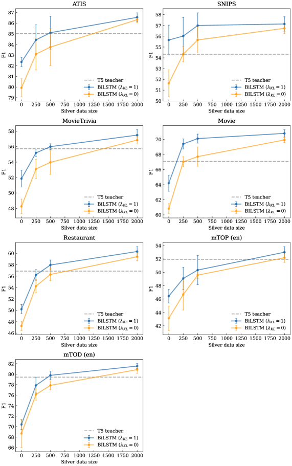
Figure 1: A graphical representation of the distillation results in Table 4(a) (100/50 gold train/dev split) as a function of the size of the silver dataset. Knowledge distillation using SenTScore generated scores outperforms pseudo-labels.

The trend with more pseudo-labeled data remains unchanged.

7 Limitations and future work

A reasonable critique to our focus on real-world constraints is the simple fact the datasets we are using are not real-world ones. From noise to tokenization choices, many issues arise when considering datasets outside of the academic domain. However, we believe our methods are simple enough to be applicable to real-world scenarios and our results to be independent of these various subtleties.

Some issues that could be addressed in future work have to do with the exploration of even larger models and different architectures such as decoder-only ones Radford et al. (2018, 2019); Brown et al. (2020); Zhang et al. (2022); Chowdhery et al. (2022); Black et al. (2021). We note, however, that in all our experiments we finetune all the weights of the pretrained models we use. When using extremely large models this becomes impractical. Recent work Turc et al. (2019) suggests that KD with compact encoder-only student models, such as BERT, is a promising avenue for further research. Exploring the pure few-shot scenario, or only finetuning a subnetwork, for instance by using adapters à la Houlsby et al., 2019, would be also interesting.

8 Conclusion

Real-time systems need to find a trade-off between performances and computing resources, the latter constraint coming either from budget or some other service requirement. Such trade-offs become particularly evident with large pretrained transformer models, which achieve SOTA results on many NLP tasks at the cost of being extremely hard and expensive to deploy in a real-world setting.

The standard solution for this is distillation. In this paper we have revisited these issues for the SL task, which is often the first crucial step in many real-world NLP pipelines. We propose a new inference algorithm, SenTScore, that allows us to leverage the performance of arbitrarily large encoder-decoder transformer architectures by distilling them into simpler sequence taggers using KD as opposed to just pseudo-labelling.

Ethical considerations

The intended use of our proposed approach is related to sequence labelling tasks where there are latency constraints and limited labelled data available. While it is not impossible to identify potential misuses of this technology, it is not immediately clear what those malicious uses would be. On the contrary, this paper contributes to the body of work investigating efficient solutions for deployment of live systems.

Computing infrastructure and computational budget

All of our experiments were run on single V100 GPU machines with 32GB. The most expensive experiments relate to finetuning a model, including best checkpoint selection. In this case, the running time is directly related to the dataset size. For the experiments using the full train/dev set, running time varies from 45 minutes (mATIS corpus) to a few hours (mTOD corpus) for a T5-base model. Training a model takes, on average, around 4 iterations per second with batch size 32. For the generation of pseudo-labels, we did not implement batch processing and it takes around 0.15 seconds to annotate each sample.

References

- (1) SLS corpora. https://groups.csail.mit.edu/sls/downloads/. Accessed: 2022-09-09.
- Artetxe et al. (2021) Mikel Artetxe, Shruti Bhosale, Naman Goyal, Todor Mihaylov, Myle Ott, Sam Shleifer, Xi Victoria Lin, Jingfei Du, Srinivasan Iyer, Ramakanth Pasunuru, Giri Anantharaman, Xian Li, Shuohui Chen, Halil Akin, Mandeep Baines, Louis Martin, Xing Zhou, Punit Singh Koura, Brian O’Horo, Jeff Wang, Luke Zettlemoyer, Mona Diab, Zornitsa Kozareva, and Ves Stoyanov. 2021. Efficient large scale language modeling with mixtures of experts.
- Athiwaratkun et al. (2020) Ben Athiwaratkun, Cicero Nogueira dos Santos, Jason Krone, and Bing Xiang. 2020. Augmented natural language for generative sequence labeling. In Proceedings of the 2020 Conference on Empirical Methods in Natural Language Processing (EMNLP), pages 375–385, Online. Association for Computational Linguistics.
- Black et al. (2021) Sid Black, Gao Leo, Phil Wang, Connor Leahy, and Stella Biderman. 2021. GPT-Neo: Large Scale Autoregressive Language Modeling with Mesh-Tensorflow. If you use this software, please cite it using these metadata.
- Brown et al. (2020) Tom Brown, Benjamin Mann, Nick Ryder, Melanie Subbiah, Jared D Kaplan, Prafulla Dhariwal, Arvind Neelakantan, Pranav Shyam, Girish Sastry, Amanda Askell, Sandhini Agarwal, Ariel Herbert-Voss, Gretchen Krueger, Tom Henighan, Rewon Child, Aditya Ramesh, Daniel Ziegler, Jeffrey Wu, Clemens Winter, Chris Hesse, Mark Chen, Eric Sigler, Mateusz Litwin, Scott Gray, Benjamin Chess, Jack Clark, Christopher Berner, Sam McCandlish, Alec Radford, Ilya Sutskever, and Dario Amodei. 2020. Language models are few-shot learners. In Advances in Neural Information Processing Systems, volume 33, pages 1877–1901. Curran Associates, Inc.
- Bucilua et al. (2006) Cristian Bucilua, Rich Caruana, and Alexandru Niculescu-Mizil. 2006. Model compression. In Proceedings of the 12th ACM SIGKDD International Conference on Knowledge Discovery and Data Mining, KDD ’06, page 535–541, New York, NY, USA. Association for Computing Machinery.
- Chowdhery et al. (2022) Aakanksha Chowdhery, Sharan Narang, Jacob Devlin, Maarten Bosma, Gaurav Mishra, Adam Roberts, Paul Barham, Hyung Won Chung, Charles Sutton, Sebastian Gehrmann, et al. 2022. Palm: Scaling language modeling with pathways. arXiv preprint arXiv:2204.02311.
- Coucke et al. (2018) Alice Coucke, Alaa Saade, Adrien Ball, Théodore Bluche, Alexandre Caulier, David Leroy, Clément Doumouro, Thibault Gisselbrecht, Francesco Caltagirone, Thibaut Lavril, Maël Primet, and Joseph Dureau. 2018. Snips voice platform: an embedded spoken language understanding system for private-by-design voice interfaces.
- De Cao et al. (2020) Nicola De Cao, Gautier Izacard, Sebastian Riedel, and Fabio Petroni. 2020. Autoregressive entity retrieval.
- Devlin et al. (2019) Jacob Devlin, Ming-Wei Chang, Kenton Lee, and Kristina Toutanova. 2019. BERT: Pre-training of deep bidirectional transformers for language understanding. In Proceedings of the 2019 Conference of the North American Chapter of the Association for Computational Linguistics: Human Language Technologies, Volume 1 (Long and Short Papers), pages 4171–4186, Minneapolis, Minnesota. Association for Computational Linguistics.
- Furlanello et al. (2018) Tommaso Furlanello, Zachary C. Lipton, Michael Tschannen, Laurent Itti, and Anima Anandkumar. 2018. Born again neural networks.
- Goo et al. (2018) Chih-Wen Goo, Guang Gao, Yun-Kai Hsu, Chih-Li Huo, Tsung-Chieh Chen, Keng-Wei Hsu, and Yun-Nung Chen. 2018. Slot-gated modeling for joint slot filling and intent prediction. In Proceedings of the 2018 Conference of the North American Chapter of the Association for Computational Linguistics: Human Language Technologies, Volume 2 (Short Papers), pages 753–757, New Orleans, Louisiana. Association for Computational Linguistics.
- Hemphill et al. (1990) Charles T. Hemphill, John J. Godfrey, and George R. Doddington. 1990. The ATIS spoken language systems pilot corpus. In Speech and Natural Language: Proceedings of a Workshop Held at Hidden Valley, Pennsylvania, June 24-27,1990.
- Hinton et al. (2015) Geoffrey Hinton, Oriol Vinyals, and Jeff Dean. 2015. Distilling the knowledge in a neural network.
- Hochreiter and Schmidhuber (1997) Sepp Hochreiter and Jürgen Schmidhuber. 1997. Long short-term memory.
- Houlsby et al. (2019) Neil Houlsby, Andrei Giurgiu, Stanislaw Jastrzebski, Bruna Morrone, Quentin De Laroussilhe, Andrea Gesmundo, Mona Attariyan, and Sylvain Gelly. 2019. Parameter-efficient transfer learning for NLP. In Proceedings of the 36th International Conference on Machine Learning, volume 97 of Proceedings of Machine Learning Research, pages 2790–2799. PMLR.
- (17) Huggingface. Models - Hugging Face.
- Jiao et al. (2020) Xiaoqi Jiao, Yichun Yin, Lifeng Shang, Xin Jiang, Xiao Chen, Linlin Li, Fang Wang, and Qun Liu. 2020. TinyBERT: Distilling BERT for natural language understanding. In Findings of the Association for Computational Linguistics: EMNLP 2020, pages 4163–4174, Online. Association for Computational Linguistics.
- Lample et al. (2016) Guillaume Lample, Miguel Ballesteros, Sandeep Subramanian, Kazuya Kawakami, and Chris Dyer. 2016. Neural architectures for named entity recognition.
- Li et al. (2021) Haoran Li, Abhinav Arora, Shuohui Chen, Anchit Gupta, Sonal Gupta, and Yashar Mehdad. 2021. MTOP: A comprehensive multilingual task-oriented semantic parsing benchmark. In Proceedings of the 16th Conference of the European Chapter of the Association for Computational Linguistics: Main Volume, pages 2950–2962, Online. Association for Computational Linguistics.
- Loshchilov and Hutter (2017) Ilya Loshchilov and Frank Hutter. 2017. Fixing weight decay regularization in adam. ArXiv, abs/1711.05101.
- Mukherjee and Hassan Awadallah (2020) Subhabrata Mukherjee and Ahmed Hassan Awadallah. 2020. XtremeDistil: Multi-stage distillation for massive multilingual models. In Proceedings of the 58th Annual Meeting of the Association for Computational Linguistics, pages 2221–2234, Online. Association for Computational Linguistics.
- Paolini et al. (2021) Giovanni Paolini, Ben Athiwaratkun, Jason Krone, Jie Ma, Alessandro Achille, Rishita Anubhai, Cicero Nogueira dos Santos, Bing Xiang, and Stefano Soatto. 2021. Structured prediction as translation between augmented natural languages.
- Pennington et al. (2014) Jeffrey Pennington, Richard Socher, and Christopher Manning. 2014. GloVe: Global vectors for word representation. In Proceedings of the 2014 Conference on Empirical Methods in Natural Language Processing (EMNLP), pages 1532–1543, Doha, Qatar. Association for Computational Linguistics.
- Qin and Joty (2021) Chengwei Qin and Shafiq Joty. 2021. Lfpt5: A unified framework for lifelong few-shot language learning based on prompt tuning of t5.
- Radford et al. (2018) Alec Radford, Karthik Narasimhan, and Tim Salimansand Ilya Sutskever. 2018. Improving language understanding by generative pre-training. https://www.cs.ubc.ca/~amuham01/LING530/papers/radford2018improving.pdf.
- Radford et al. (2019) Alec Radford, Jeffrey Wu, Rewon Child, David Luan, Dario Amodei, and Ilya Stuskever. 2019. Language models are unsupervised multitask learners. Technical report, OpenAI.
- Raffel et al. (2020) Colin Raffel, Noam Shazeer, Adam Roberts, Katherine Lee, Sharan Narang, Michael Matena, Yanqi Zhou, Wei Li, and Peter J. Liu. 2020. Exploring the limits of transfer learning with a unified text-to-text transformer. Journal of Machine Learning Research, 21(140):1–67.
- Raman et al. (2022) Karthik Raman, Iftekhar Naim, Jiecao Chen, Kazuma Hashimoto, Kiran Yalasangi, and Krishna Srinivasan. 2022. Transforming sequence tagging into a seq2seq task.
- Schuster et al. (2019) Sebastian Schuster, Sonal Gupta, Rushin Shah, and Mike Lewis. 2019. Cross-lingual transfer learning for multilingual task oriented dialog. In Proceedings of the 2019 Conference of the North American Chapter of the Association for Computational Linguistics: Human Language Technologies, Volume 1 (Long and Short Papers), pages 3795–3805, Minneapolis, Minnesota. Association for Computational Linguistics.
- Shleifer and Rush (2020) Sam Shleifer and Alexander M. Rush. 2020. Pre-trained summarization distillation.
- (32) StanfordNLP. GloVe: Global Vectors for Word Representation.
- Tang et al. (2019) Raphael Tang, Yao Lu, Linqing Liu, Lili Mou, Olga Vechtomova, and Jimmy Lin. 2019. Distilling task-specific knowledge from bert into simple neural networks.
- Tjong Kim Sang and De Meulder (2003) Erik F. Tjong Kim Sang and Fien De Meulder. 2003. Introduction to the CoNLL-2003 shared task: Language-independent named entity recognition. In Proceedings of the Seventh Conference on Natural Language Learning at HLT-NAACL 2003, pages 142–147.
- Turc et al. (2019) Iulia Turc, Ming-Wei Chang, Kenton Lee, and Kristina Toutanova. 2019. Well-read students learn better: On the importance of pre-training compact models.
- Xue et al. (2022) Linting Xue, Aditya Barua, Noah Constant, Rami Al-Rfou, Sharan Narang, Mihir Kale, Adam Roberts, and Colin Raffel. 2022. Byt5: Towards a token-free future with pre-trained byte-to-byte models. Transactions of the Association for Computational Linguistics, 10:291–306.
- Xue et al. (2021) Linting Xue, Noah Constant, Adam Roberts, Mihir Kale, Rami Al-Rfou, Aditya Siddhant, Aditya Barua, and Colin Raffel. 2021. mT5: A massively multilingual pre-trained text-to-text transformer. In Proceedings of the 2021 Conference of the North American Chapter of the Association for Computational Linguistics: Human Language Technologies, pages 483–498, Online. Association for Computational Linguistics.
- Yan et al. (2021) Hang Yan, Tao Gui, Junqi Dai, Qipeng Guo, Zheng Zhang, and Xipeng Qiu. 2021. A unified generative framework for various NER subtasks. In Proceedings of the 59th Annual Meeting of the Association for Computational Linguistics and the 11th International Joint Conference on Natural Language Processing (Volume 1: Long Papers), pages 5808–5822, Online. Association for Computational Linguistics.
- Zhang et al. (2022) Susan Zhang, Stephen Roller, Naman Goyal, Mikel Artetxe, Moya Chen, Shuohui Chen, Christopher Dewan, Mona Diab, Xian Li, Xi Victoria Lin, Todor Mihaylov, Myle Ott, Sam Shleifer, Kurt Shuster, Daniel Simig, Punit Singh Koura, Anjali Sridhar, Tianlu Wang, and Luke Zettlemoyer. 2022. Opt: Open pre-trained transformer language models.