Abstract

Neuroscientific studies aim to find an accurate and reliable brain Effective Connectome (EC). Although current EC discovery methods have contributed to our understanding of brain organization, their performances are severely constrained by the short sample size and poor temporal resolution of fMRI data, and high dimensionality of the brain connectome. By leveraging the DTI data as prior knowledge, we introduce two Bayesian causal discovery frameworks -the Bayesian GOLEM (BGOLEM) and Bayesian FGES (BFGES) methods- that offer significantly more accurate and reliable ECs and address the shortcomings of the existing causal discovery methods in discovering ECs based on only fMRI data. Through a series of simulation studies on synthetic and hybrid (DTI of the Human Connectome Project (HCP) subjects and synthetic fMRI) data, we demonstrate the effectiveness of the proposed methods in discovering EC. To numerically assess the improvement in the accuracy of ECs with our method on empirical data, we first introduce the Pseudo False Discovery Rate (PFDR) as a new computational accuracy metric for causal discovery in the brain. We show that our Bayesian methods achieve higher accuracy than traditional methods on HCP data. Additionally, we measure the reliability of discovered ECs using the Rogers-Tanimoto index for test-retest data and show that our Bayesian methods provide significantly more reproducible ECs than traditional methods. Overall, our study’s numerical and graphical results highlight the potential for these frameworks to advance our understanding of brain function and organization significantly.

Introduction

Causal connectivity, also known as the Effective Connectome (EC), empowers us to better understand brain functionality compared to functional connectivity, which is the temporal correlation of neuronal activity of the brain regions [1]. Dynamic Causal Modeling (DCM) [2], Partial Correlation Thresholding (PCT) [3], Bayesian networks [4], Granger Causality (GC) [5], and Structural Equation Models (SEM) [6] are fundamental methods to investigate the causal connectivity in the brain that reveals neuroscientific insights for researchers. The graphical approaches, among all others, have shown to be more effective in extracting causality from observational and experimental data [7, 8]. Graphical approaches, or the Directed Acyclic Graph (DAG) framework, focus on identifying the underlying mechanism based on observational and experimental data. These approaches can be viewed as the reverse of the DCM’s procedure, in which the model is built on our understanding of the physiological underpinnings of the BOLD response [9]. As a graphical approach, the Fast Greedy Equivalent Search (FGES) [10], NOTEARS [11], and Gradient-based Optimization of DAG-penalized Likelihood for learning linEar DAG Models (GOLEM) [12] are more accurate in large-scale networks, which makes them more appropriate in discovering EC. While in [9] and [13], the effectiveness of the FGES and NOTEARS methods in discovering ECs are illustrated; however, extracting causality in high-dimensional graphs is still challenging, and the accuracy of the derived graph decreases significantly as the network size grows and the sample size becomes limited, as demonstrated in [12]. Furthermore, as it is shown [14, 15], analyzing brain connectivity using unimodal data presents fundamental ambiguities such as low the reproducibility of discovered ECs. In [16], it is shown that prior information that favors sparsity (such as DTI signals [17]) can significantly enhance both the accuracy and reproducibility of discovered graphs when a limited amount of data (such as fMRI signals) is available and the dimension of networks grows (such as brain network). Therefore, developing Bayesian causal methods based on multimodal data may help overcome the abovementioned obstacles.

The recent research on multimodal data indicates that the anatomical structure constrains the strength and persistence of effective/functional connectivities [23, 24, 18, 20, 19, 21, 22]. However, the results in [25, 26] suggest that while there is some degree of overlap between functional and structural connectivity, there are also cases in which they may not align perfectly. The main reason for this misalignment is that functional connectivity refers to the statistical dependencies between different brain regions. Contrary to functional connectivity, in the context of causal inference, it is well-studied that causal connectivity completely aligns with structural connectivity, i.e., a causal connection between two regions cannot be discovered without the mediation of another variable if the structural connection does not exist. Additionally, the left and right hemispheres of the brain share information through commissural nerve tracts. As a result, to ensure that other nodes are not mediating or confounding factors in the brain network, it is essential to include the subcortical regions nodes to satisfy the causal sufficiency assumption presented in [8]. Studies such as [27] have shown that developing Bayesian frameworks for discovering ECs improves inference on effective connectivity, compared with unimodal studies. This research path has garnered significant attention in neuroscience and shows promise in understanding brain organization. Notably, as a causal modeling approach, the DCM method benefits significantly from extracting effective connections with priors on structural connectivity. In [28] and [29], the ECs for patients with depression and autism, respectively, are extracted by focusing on the structurally connected regions. Specifically, they apply a linearized version of the DCM to only the structurally connected regions. In [30, 31], the authors presented a Bayesian DCM method using probabilistic structural connectivity (SC) as prior information. The derived results in these studies are compared with fMRI-based models to illustrate the improvement of the accuracy of the EC model when SC is employed as prior information. Moreover, causality in the brain is investigated in [32] with the Bayesian partial correlation method, in which the DTI data is approximated with the G-Wishart distribution as the conjugate prior. Likewise, in [33], the authors investigate causality by minimizing the reconstruction error of an autoregressive model constrained by the structural connectivity prior.

In this paper, we introduce two new Bayesian causal frameworks, i.e., Bayesian GOLEM (BGOLEM) and Bayesian FGES (BFGES), using DTI data as prior knowledge of the EC discovery to address the mentioned concerns. Then, we show that these frameworks provide more accurate and reliable (reproducible) ECs that highlight the potential for these frameworks to advance our understanding of brain function and organization significantly. The traditional method for assessing the accuracy of causal discovery methods is to compare the ECs discovered from the patient and normal subjects’ data [13, 28, 29]. While this approach can be informative about causal interactions in brain networks, the agreement/disagreement of small parts of ECs of patient and normal subjects does not necessarily imply the accuracy/inaccuracy of a causal method. We present the Pseudo False Discovery Rate (PFDR) metric based on the False Discovery Rate (FDR) as a computational metric in evaluating the accuracy of discovered ECs without the drawbacks of the need for patient and normal subjects comparison.

The main contributions of our work are three-fold:

• First, we introduce the BGOLEM and BFGES methods as Bayesian causal frameworks to improve the accuracy and reliability of discovering brain effective connectomes while addressing existing practical and computational concerns. These methods are Bayesian extensions of well-established GOLEM and FGES methods.

• Second, we introduce the concept of the Pseudo FDR (PFDR) metric to demonstrate the necessity of multimodal analysis, illustrate the effectiveness of Bayesian causal frameworks, adjust each method’s hyperparameters, and compare the accuracy of different methods.

• Third, we demonstrate that our Bayesian methods for discovering ECs achieve higher accuracy as computed with the PFDR metric and greater reliability as assessed by the reproducibility metric known as the Roger-Tanimoto index. The numerical and graphical results highlight the potential of our frameworks to significantly advance our understanding of brain function and organization.

The rest of the paper is organized as follows.  Materials and methods section presents our Bayesian frameworks, BGOLEM and BFGES methods, and our proposed computational accuracy measure, the PFDR. In  Results section, we utilize the developed methods with the hybrid data and illustrate the effectiveness of Bayesian methods by comparing different types of errors. Then, we employ Bayesian causal frameworks with HCP data and assess the accuracy and reliability of the discovered ECs through various tools. Finally, we discuss the results and limitations of our methods. Fig 1 shows the schematic of our contributions and methods.

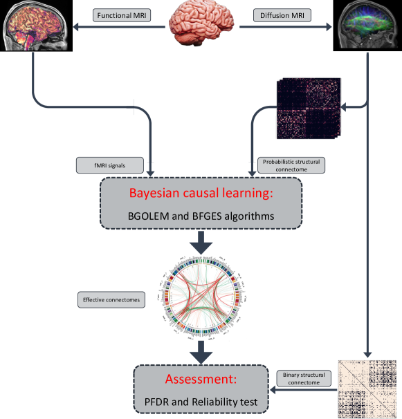
Fig 1: Steps in Bayesian causal learning and Assessment of effective connectomes. Deriving effective connectomes for both hybrid and empirical data with introduced Bayesian causal frameworks, computing the PFDR value and performing reliability tests

Materials and methods

In this section, we introduce our Bayesian causal frameworks, BGOLEM and BFGES, based on GOLEM and FGES methods. Then, we present the concept of the PFDR metric, with an eye on the idea from the DTI technique and the FDR metric. The empirical and hybrid data are presented at the end of this section.

Bayesian causal discovery frameworks

Consider a parameterized Bayesian network model with $n$ nodes ($B$), defined by $(G,\theta)$, where, $G=(V,E)$ is a DAG, $V$ is a set of nodes ($U=\{X_{1},...,X_{n}\}$), $E$ is a set of directed edges (causal relations), and $\theta$ is a set of parameters that specify all conditional probability distributions. A parameterized Bayesian network $B$ represents and factors a joint distribution over $U$ according to the structure $G$

$$P_{B}(X_{1},...,X_{n})=\prod_{i=1}^{n}{p(X_{i}=x_{i}|Pa^{G}_{i}=pa^{G}_{i},\theta_{i})}$$ (1)

where $Pa^{G}_{i}$ is the set of parents of $X_{i}$ in $G$, and $\theta_{i}\subset\theta$ is the subset of parameters that define the conditional probability of node $X_{i}\in V$ given its parents in $G$.

Proposed Bayesian GOLEM method

The GOLEM algorithm finds a linear DAG model that equivalently represents a set of linear structural equations. In GOLEM, $P_{B}$ in equation 1 is generated by the linear DAG, $X=WX+N$, where, $X=[X_{1},...,X_{n}]^{T}$, $W$ is a $n\times n$ weighted adjacency matrix, and $N=[N_{1},...,N_{n}]^{T}$ is an independent noise vector. In [11], $W$ matrix is found by optimizing a score function $F_{B}(W,X)$, subject to the structure $G$, for a given samples $X$

$$\min_{W\in R^{n\times n}}\quad F_{B}(W,X)$$

s.t. $$G(W)\in DAGs$$

$$F_{B}(W,X) =l(W,X)+R_{sparse}(W)$$ (2)

where $G(W)$ is the $n$-node graph induced by the weighted adjacency matrix $W$ and $F_{B}(.):R^{n\times n}\rightarrow R$ is the score function. $l(W,X)$ is the maximum likelihood, $R_{sparse}(W)$ is a penalty term that favors sparsity, i.e., having fewer edges. The hard optimization problem in equation 2 is relaxed into a soft optimization problem presented in [12] as follows

$$\min_{W\in R^{n\times n}}\quad S_{B}(W,X)$$

$$S_{B}(W,X) =F_{B}(W,X)+R_{DAG}(W)$$

$$=l(W,X)+R_{sparse}(W)+R_{DAG}(W)$$ (3)

where $R_{DAG}(W)$ is a penalty term that favors DAGness of $W$. The penalty term for encouraging sparsity is defined as $\lambda\lVert{W}\rVert$. The details of the algorithm and proofs are found in [12].

BGOLEM

According to [12], the GOLEM method results in lower Structural Hamming Distance (SHD) and FDR values for the sparse structures. Moreover, for a limited sample size, the accuracy of GOLEM significantly decreases with a higher number of edges and nodes. To cope with this deficiency, we define the BGOLEM algorithm by suggesting the following sparsity penalty term in 3, to include the prior probability

$$R_{sparse}(W)=\lambda\Big{\|}Q\bigl{(}P(G),W\bigl{)}\Big{\|}$$ (4)

where $Q(.):R^{n\times n}\times R^{n\times n}\rightarrow R^{n\times n}$ is a smooth element-wise monotonic function. This function acts element-wise on the input matrices, such that if a specific element in the $P(G)$ matrix moves in one direction, the corresponding element of the $W$ moves in the same direction. Such a sparsity penalty term inhibits/excite an element of the $W$ matrix that has a lower/higher prior probability. In this paper, we have considered

$$Q\bigl{(}P(G),W\bigl{)}=\log\bigl{(}{P(G)}\bigl{)}\odot{W}$$ (5)

where $\odot$ is the element-wise matrix product. The way that the prior knowledge incorporates into the method depends on our choice of function in equation 5. To find a proper $\lambda$ value, an exhaustive search can be performed to find the optimum $\lambda$ value with the lowest false discovery rate. However, for fMRI data, since there is no access to the ground truth, we use the PFDR metric that is presented in section The PFDR metric to find the optimum $\lambda$ value.

Proposed Bayesian FGES method

The FGES causal discovery method presented in [10], has two main parts that are: how the algorithm operates and how to define the scoring criteria. This algorithm has two steps and starts with an empty graph. In the first step, the forward phase, scores of all alternative one-edge additions to the graph are computed. The edge that corresponds with the best score is added to the graph. This process continues until no more improvement is achieved by adding a single edge. In the second step, the backward stage, the graph is pruned backward elimination through step-wise single-edge deletion. This procedure continues until any single-edge deletion results in a decline in the score. The FGES uses a decomposable score. Where there is no need to compute the score of the entire graph in each iteration. Only the scores of the nodes with changing parents change. This is the main difference between the FGES and GES methods [34, 10]. The decomposable scoring criteria $S_{B}$ [10], is defined by

$$S_{B}(G,D)=\sum_{i=1}^{n}{s(X_{i},Pa^{G}_{i})}$$ (6)

where $D$ is a set of observed data and $s_{B}(X_{i},Pa^{G}_{i})$ is the score corresponding to a node $X_{i}$ and its parents $Pa^{G}_{i}$.

The Bayesian score function $S_{B}$ using the relative log posterior of $G$ is

$$S_{B}(G,D)=\log{p(G)}+\log{p(D|G,\theta)}$$ (7)

where $p(G)$ is the prior probability of $G$, and $p(D|G)$ is the conditional likelihood of $D$ [10]. In particular, in [35], the authors show that equation 7 for curved exponential models can be approximated using Laplace’s method for integrals, yielding

$$S_{B}(G,D)\approx\log{p(G)}+\log{p(D|G,\hat{\theta})}-\frac{d}{2}\log(m)$$ (8)

where $\hat{\theta}$ denotes the maximum-likelihood estimate for the network parameters, $d$ denotes the dimension (i.e., number of free parameters) of $G$, and $m$ is the number of records in $D$. In [10], the decomposable score for the FGES method is defined by the sum of the second and third terms in equation 8 that is also known as the BIC, i.e.,

$$S_{B}(G,D)=\sum_{i=1}^{n}{\bigl{(}\log{p(X_{i}|\hat{\theta_{i}},Pa_{i}^{G})}-\lambda\frac{d_{i}}{2}\log(m)\bigl{)}}$$ (9)

where $\lambda$ is the hyperparameter of the BIC score.

BFGES

Similar to the GOLEM method, the FGES method has difficulties in discovering DAGs with higher number of nodes and edges, and a limited number of samples, as illustrated in [11]. While the $\log{p(G)}$ term is neglected in the BIC scoring 9, this term can play a dominant role in model selection of large scale graphs [16]. In our proposed Bayesian FGES algorithm, considering the equations 6 and 7, we derive the decomposable version of equation 8 as follows

$$\begin{split}S_{B}(G,D)&=\log{p(G)}+\sum_{i=1}^{n}{s_{B}(X_{i},Pa^{G}_{i})}\\ &=\log{p(G)}+\sum_{i=1}^{n}{\bigl{(}\log{p(X_{i}|\hat{\theta_{i}},Pa_{i}^{G})}-\lambda\frac{d_{i}}{2}\log(m)\bigl{)}}\end{split}$$ (10)

where $d_{i}$ denotes the number of parameters for the structure of $X_{i}$ and its parents. The procedure of deriving equation 10 is quite similar to that of equation 9, but without ignoring the prior probability. If we assume a uniform prior for the existence of an edge, all three probabilities of $X_{i}\leftarrow X_{j}$, $X_{i}\rightarrow X_{j}$ and $X_{i}\dots X_{j}$ ($X_{i}$ and $X_{j}$ are not connected) are equal to $\frac{1}{3}$. Since the probability of $X_{i}$ not being a parent of “$X_{j}$ is equal to $\frac{2}{3}$”, then ${p(G)}={\frac{1}{3}}^{N_{G}}\times{\frac{2}{3}}^{\bigl{(}\frac{(n^{2}-n)}{2}-N_{G}\bigl{)}}$, where $N_{G}$ an $n$ are the number of edges and number of nodes in graph $G$, respectively. Similar to the FGES algorithm, in the BFGES algorithm, we start with an empty graph, which means that $p(G)$ is the probability of a graph $G$ with no edges. As a result, the algorithm starts with

$$\begin{split}p(G)=\prod_{i=1}^{n}{\prod_{j=1}^{n}{\bigl{(}1-p(X_{i}\leftrightarrow X_{j}})\bigl{)}}\end{split}$$ (11)

where $p(X_{i}\leftrightarrow X_{j})=p(X_{i}\rightarrow X_{j})+p(X_{i}\leftarrow X_{j})$ is the edge existence probability between nodes $i$ and $j$, $i\neq j$. Consequently, effect of adding an edge from node $i$ to node $j$ is to subtract $\log\bigl{(}1-p(X_{i}\leftrightarrow X_{j})\bigl{)}$ from the score and add $\log\frac{1}{2}p(X_{i}\leftrightarrow X_{j})$ to the score

$$\begin{split}S_{B}(G^{{}^{\prime}},D)=S_{B}(G,D)-\log\bigl{(}1-p(X_{i}\leftrightarrow X_{j})\bigl{)}+\log\frac{1}{2}p(X_{i}\leftrightarrow X_{j})\end{split}$$ (12)

where in this equation, $S_{B}(G^{{}^{\prime}},D)$ is the score of graph $G^{{}^{\prime}}$ that is derived from adding $X_{i}\rightarrow X_{j}$ to graph $G$.

In the backward stage of the BFGES algorithm, the score of the derived graph is subtracted with $\log\frac{1}{2}p(X_{i}\leftrightarrow X_{j})$ and $\log\bigl{(}1-p(X_{i}\rightarrow X_{j})\bigl{)}$ is added when the edge from node $j$ to $i$ is eliminated

$$\begin{split}S_{B}(G^{{}^{\prime}},D)=S_{B}(G,D)+\log\bigl{(}1-p(X_{i}\leftrightarrow X_{j})\bigl{)}-\log\frac{1}{2}p(X_{i}\leftrightarrow X_{j})\end{split}$$ (13)

where $S_{B}(G^{{}^{\prime}},D)$ is the score of graph $G^{{}^{\prime}}$ that is derived from removing $X_{i}\rightarrow X_{j}$ from graph $G$.

In sum, the BFGES algorithm runs similar to the FGES algorithm with the modified scoring 10 to incorporate prior knowledge in causal discovery. Similar to the BGOLEM method, for fMRI data, we use the PFDR metric (section The PFDR metric) to find the optimum $\lambda$ value.

The PFDR metric

To measure the reliability of methods in discovering causality, False Discovery Rate (FDR) is a powerful full metric to assess the accuracy of discovered edges, which is defined as follows

$$\textrm{FDR}=\frac{FP}{NoDE}$$ (14)

where $FP$ and $NoDE$ are the number of False Positives and the Total Number of Discovered Edges, in the true underlying EC, respectively [36]. In the assessment of discovered ECs, there is no access to the true causal underlying graph. As a result, computing $FP$ and consequently, FDR value is not possible.

In the DTI technique, the relative diffusivity of water in a voxel into directional components is quantified. The longest axis of the diffusion ellipsoid, which is estimated based on diffusion tensors, is used to track nerve fibers as they travel between potentially functionally associated brain regions [37]. The absence of an edge in SC indicates that there is no physical connection between two regions which implies that no effective connection is possible. On the other hand, the existence of an edge in this matrix implies a physical path between two regions, which opens the door for effective connectivity. Therefore, from the absence of an edge in this matrix, one can infer that the corresponding element of the EC must be zero. The presence of an edge in SC allows for corresponding non-zero element in EC. We exploit DTI-based SC information and propose the Pseudo FDR (PFDR) metric, which is defined as follows

$$\textrm{PFDR}=\frac{FP^{{}^{\prime}}}{{FP^{{}^{\prime}}}+TP^{{}^{\prime}}}$$ (15)

where $FP^{{}^{\prime}}$ is the number of edges that are one in EC and zero in SC and $TP^{{}^{\prime}}$ is the number of edges that are one in both EC and SC. From the definition of $FP$ and $FP^{{}^{\prime}}$, false positives in PFDR computations are a subset of true false positives in FDR computation, as a result, $FP^{{}^{\prime}}\leq FP$. Contrary to the FDR metric, computing the PFDR metric is practicable, while we do not know the true underlying graph. This metric enables us to measure and compare the accuracy of the ECs discovered with causal discovery methods. The PFDR can be used to adjust the hyperparameters of causal discovery methods, as well. In section Results for the empirical data, we experimentally explore the relation between FDR and PFDR. Details and discussions on Pseudo FDR can be found in Appendix 1.

Probabilistic structural connectome

The prior knowledge in the developed Bayesian methods are computed from DTI data. As a result, in order to compute the probabilistic SC $(P_{SC})$, we use the following formula

$$\rho^{*}_{ij}=\frac{\rho_{ij}}{\sum_{j=1}^{j=n}{\rho_{ij}}}$$ (16)

where $\rho_{ij}$ represents the streamlines from seed $i$ to the target region $j$ that is normalized according to the area of the $j^{th}$ region [30] and $n$ is number of regions in brain atlas.

Data

Data acquisition

In this study, we used DWI and fMRI data from unrelated subjects of the “HCP1200” data set (March 2017 data release of healthy adults aged 22–35) [38] along with the synthetic fMRI signals that are generated with DTI-based DAGs. The HCP data sets were acquired using protocols approved by the Washington University institutional review board, and written informed consent was obtained from all subjects.

DTI data preprocessing

DWIs were acquired using a 3T ‘Connectome Skyra’, provided with a Siemens SC72 gradient coil and stronger gradient power supply with maximum gradient amplitude (Gmax) of 100 $mT/m$ (initially 70 $mT/m$ and 84 $mT/m$ in the pilot phase) sequence and 90 gradient directions equally distributed over 3 shells (b-values 1000, 2000, 3000 $mm/s^{2}$) with 1.25mm isotropic voxels [39]. We process this data by MRtrix3 [40]and with 50 million streamlines, the tractograms are generated. Then, the results are normalized with the volume of parcelled regions.

Parcellation

In order to ensure the causal sufficiency assumptions [8], we have included subcortical regions in our computations because the information flow originated from the brain stem are fed to these regions. This means that these regions could be ancestors of cortex regions and could play the role of the confounding variable for them. Let us assume that region A includes $a_{1}$ and $a_{2}$ sectors and region $B$ contains $b_{1}$ and $b_{2}$ sectors. Sector $a_{1}$ may have a causal influence on sector $b_{1}$ and sector $b_{2}$ has a causal influence on sector $a_{2}$. The causal discovery procedure can be interrupted due to situations like this As a result, it is important to choose an atlas that has a rich number of regions. Correspondingly, we employ the Destrieux atlas [41] that satisfies our concerns. The List of ROIs of the Destrieux atlas is presented in Appendix 2.

Hybrid data

We have generated two groups of data sets. We employ SF7 data generation in [11], which has degree of 7, with $[50,75,100,125,150]$ number of nodes and 300 time points to compare the results and effectiveness of our Bayesian methods with the results in [12]. The hybrid data, the second group of data, is generated based on the DTI data of 50 unrelated subjects of the HCP and the Hemodynamic response function. We generate 50 networks with 164 nodes based on the DAGs that are created from the HCP DTI data. The existence of an edge in each network is the result of a Bernoulli distribution that the parameter of this distribution is the element of SC, which is derived from the DTI data of HCP. The number of time points is 1200, which is similar to fMRI data of HCP and number of edges is 1000. More details on the generation of Hybrid data can be found in Appendix 1.

Emperical data

The HCP MRI data acquisition protocols and procedures have previously been described in full detail [42]. We used the minimally preprocessed images of ‘rsfMRI’ and ‘dMRI’ for 50 unrelated subjects that were provided by the HCP S1200 Release. fMRI resting-state runs (HCP file name: rfMRI-REST1 and rfMRI-REST2) were acquired in four separate sessions on two different days, with two different acquisitions (left to right, or LR, and right to left, or RL) per day [43]. In our simulations, we use the mean of two sessions ( right to left and left to right) to avoid biases. Mean of two sessions of the second day is employed as retest data. In both empirical and hybrid data, we use DTI data of the same subjects.

Results

The probabilistic SCs are computed from equation 16. To derive the binary SC, number of tracts for each subject is binarized at $50\%$ threshold of stream counts. The majority voting is applied to the 50 binary matrices to compute the final binary SC that we use in the PFDR. This threshold value is chosen to derive a conservative SC, in which there is a high degree of confidence in the zero values of this matrix. The extracted binary SC has $33\%$ zero elements.

In the following, with the assistance of the derived binary and probabilistic SCs, we apply the GOLEM and FGES methods along with our proposed frameworks, the BGOLEM and BFGES, to hybrid and empirical data. In Bayesian causal frameworks, we employ the probabilistic SC of each subject as a prior knowledge of the EC discovery of the same subject. Results for hybrid data for all 4 methods are derived with adjusting $\lambda$ according to the minimum of FDR values for the test data. The ECs of empirical data are derived with adjusting $\lambda$ according to the PFDR values for test data. The PFDR for each subject is computed based on the binary SC that is derived from excluding the same subject from 50 subjects.

Results for the hybrid data

The results of applying the FGES and BFGES methods as well as the GOLEM and BGOLEM methods on data with different number of nodes are illustrated in Fig 2.

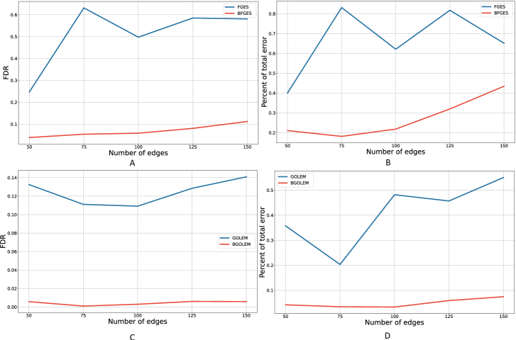
Fig 2: The FDR and percent of total errors for graphs with different number edges. A: The FDR for the GOLEM and BGOLEM methods B: Percent of total errors for the GOLEM and BGOLEM methods C: The FDR for the FGES and BFGES methods D: Percent of total errors for the FGES and BFGES methods

In the first row of Fig 2, the FDR and percent of total errors,

$$\frac{False\ Positives+False\ Negatives}{Total\ Number\ of\ Discovered\ Edges}$$ (17)

, are shown for both GOLEM and BGOLEM methods. The same error ratios are shown for FGES and BFGES methods in the second row of this figure. The results of applying FGES and BFGES are derived with $\lambda=[9,8,6,4,5]$ and $\lambda=[0.3,1,0.3,0.4,0.1]$ for SF7 data with $50$, $75$, $100$, $125$ and $150$ nodes, respectively. The errors for BGOLEM and GOLEM methods are derived with $\lambda=[0.01,0.01,0.012,0.009,0.01]$ and $\lambda=[0.008,0.009,0.009,0.01,0.0.008]$ for the same group of data, respectively.

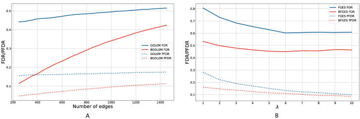
Fig 3: Dependency of the PFDR and FDR metrics in both causal frameworks. A: The correlation coefficients ($R$) of PFDR and FDR values for the ECs of the GOLEM and BGOLEM are $98.9\%$ and $99.9\%$, respectively B: The correlation coefficients of PFDR and FDR values for FGES and BFGES are $80.9\%$ and $97.7\%$, respectively.

Fig 3 illustrates the effect of employing the Bayesian frameworks on hybrid fMRI data with 164 nodes that are created from randomly generated DAGs based on the DTI data of HCP. In plot A, the FDR and PFDR values of ECs with different thresholds on the number of edges for the GOLEM and BGOLEM methods are shown. The correlation coefficients ($R$) of PFDR and FDR values for the ECs of the GOLEM and BGOLEM are $98.9\%$ and $99.9\%$, respectively. In plot B, the FDR and PFDR values for the FGES and BFGES ECs are illustrated for different $\lambda$ values. The correlation coefficients of PFDR and FDR values for FGES and BFGES are $80.9\%$ and $97.7\%$, respectively.

Results for the empirical data

In this section, we present and compare the results of applying our methods and traditional methods to empirical data, both graphically and computationally.

In Fig 4, structural connectome, correlation-based connectome and ECs discovered with the FGES, BFGES, GOLEM and BGOLEM methods are shown for 148 regions of the left and right hemispheres. To clearly illustrate the edges between the two hemispheres, 16 subcortical regions are excluded in this figure.

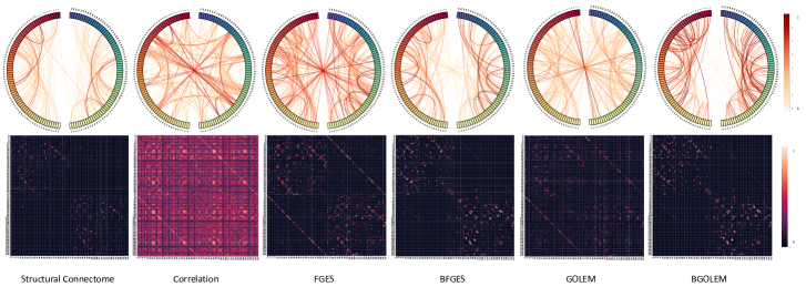
Fig 4: Comparison of Structural connectome, correlation-based connectome and ECs discovered with the FGES, BFGES, GOLEM and BGOLEM methods. The first row compares the symmetry of structural connectomes, correlation-based, and ECs and edges between two hemispheres of each connectome. Second row, compares the results of ECs discovered with SC, correlation-based connectome, and ECs of non-Bayesian methods.

To numerically investigate the accuracy and reliability of the ECs shown in Fig 4, first, we employ the PFDR as an accuracy metric and then, we use the Roger Tanimoto index as a reproducibility metric.

The mean PFDRs for different numbers of edges are presented for the FGES, GOLEM, BFGES and BGOLEM methods in Fig 5. In Fig 5.A, the PFDR values for ECs discovered with the FGES and GOLEM methods are shown, for different numbers of edges. The lowest mean PFDR value for the FGES method is $24.6\%$ for the penalty coefficient between $4$ and $6$. The lowest value of the mean PFDR of the GOLEM method is between $[12,17.2]\%$ for the different number of edges and variation of $\lambda$. The mean PFDR values for ECs of the BGOLEM and BFGES methods are derived with respect to their lowest mean PFDRs and shown in Fig 5.B. The PFDR values of ECs are $[12.1-15.2]\%$ and $[3-3.3]\%$ for BFGES and BGOLEM methods, respectively. More analyses and results on empirical data, the schematic of SCs and the effect of $\lambda$ variation on the PFDR of empirical data can be found in Appendix 1.

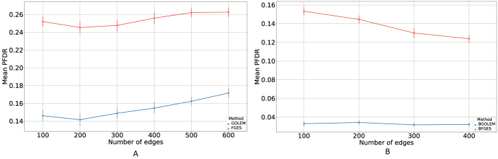
Fig 5: The PFDRs for the ECs discovered with the GOLEM, FGES, BGOLEM, and BFGES methods. A: The PFDR for ECs with the best hyperparameters of the GOLEM and FGES methods B: The PFDR of ECs with the best hyperparameters of BGOLEM and BFGES methods

In table LABEL:table:1, we compare the PFDR values for the Mean 1 (test) and Mean 2 (retest) data when 200 edges are selected. In this table, Mean 1 is the mean of LR and RL data of 50 subjects acquired on the first day and Mean 2 is the mean for the data acquired on the second day.

Table 1: Effect of applying Bayesian methods on mean PFDR values for ECs with 200 edges for test and retest data and

	Data
Method	Mean 1	Mean 2
FGES	$0.242\pm 0.0035$	$0.254\pm 0.0042$
BFGES	$0.142\pm 0.0015$	$0.154\pm 0.0022$
GOLEM	$0.141\pm 0.0022$	$0.132\pm 0.0015$
BGOLEM	$0.024\pm 0.0002$	$0.31\pm 0.0003$

The PFDR metric compares the accuracy of each method in parts of the discovered ECs that are zero in the SC and there is still no ground truth about the part that is one in the SC. To evaluate the EC edges that are one in the SC, for the ECs with 200 edges, we apply the proportion test [44] to compare each edge of ECs that are discovered with the GOLEM and FGES methods. This test is designed to determine whether the proportion of each edge in the ECs of 50 subjects derived using FGES methods is equal to the proportion of the corresponding edge in the ECs obtained using GOLEM methods. The ratio of the number of noticeably different edges in the EC portions with structural edges of one to those with structural edges of zero is then computed. In comparing these two methods, $11.2\%$ of edges are different in the ECs for the edges that are one in SC, on the other hand, $40.3\%$ of edges are different in the ECs for the edges that are zero in SC.

To further investigate the effectiveness of the Bayesian causal frameworks on the reliability of discovered directed ECs, we use the Rogers-Tanimoto index to evaluate the reproducibility of the developed methods. This index is zero for the edge that is zero or one in all subjects. The Rogers-Tanimoto index [45] investigates the dissimilarity of each discovered directed edge between 50 subjects. In Fig 6, we demonstrate the Roger-Tanimoto values of the ECs with 164 regions extracted with Bayesian and non-Bayesian methods for test and retest data. In this figure, this index is computed for both symmetric and asymmetric edges.

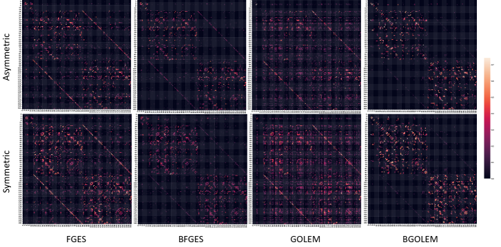
Fig 6: Comparing the effect of employing Bayesian and non-Bayesian methods in the reproducibility of discovered asymmetric and symmetric ECs.

Fig 7 shows the numerical values of the Rogers-Tanimoto index for all the directed edges discovered with the GOLEM, BGOLEM, FGES, and BFGES for test and retest data. The median and interquartile range of the Rogers-Tanimoto index for directed ECs of the FGES method are $4\%$ and $[4,11.5]\%$. These values for the directed ECs of the GOLEM methods are $4\%$ and $[4,11.4]\%$. The median and interquartile range for the BFGES method are $4\%$ and $[0,7.8]\%$, and for the BGOLEM method, these values are $0\%$ and $[0,4]\%$. The Rogers-Tanimoto index is computed for the directed ECs discovered with the FGES, BFGES, GOLEM, and BGOLEM methods that have roughly 200 edges. The Rogers-Tanimoto index for undirected ECs is illustrated and discussed in Appendix 1.

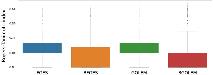
Fig 7: The box plots of the Rogers-Tanimoto values of the FGES, BFGES, GOLEM, BGOLEM. The median and interquartile range of the Rogers-Tanimoto index for directed ECs of the FGES method are $4\%$ and $[4,11.5]\%$. These values for the directed ECs of the GOLEM methods are $4\%$ and $[4,11.4]\%$. The median and interquartile range for the BFGES method are $4\%$ and $[0,7.8]\%$, and for the BGOLEM method, these values are $0\%$ and $[0,4]\%$.

Discussion

In this paper, first, the Bayesian causal frameworks are introduced in sections Proposed Bayesian GOLEM method and Proposed Bayesian FGES method. The PFDR metric is presented in section The PFDR metric as a computable alternative for the FDR metric to assess the accuracy of causal discovery methods.

Fig 2 shows that the FDR and percent of total error are improved with the employment of Bayesian causal frameworks for SF7 data with different number of nodes. The results of applying the FGES and GOLEM methods to this data are consistent with the results in [12]. Fig 3, shows the relationship between FDR and PFDR using hybrid fMRI data. The correlation coefficient between the PFDR and FDR of ECs obtained using the BGOLEM, GOLEM, BFGES, and FGES methods on hybrid fMRI data with 164 nodes are close to one, i.e., the PFDR and FDR values are highly correlated in all of the methods. These results justify the trustworthiness of the PFDR metric.

Fig 4 compares the structural, functional, effective, and Bayesian effective connectomes in various aspects. This figure investigates the symmetry of connections in the two hemispheres and the edges between them. Comparison between the functional connectome derived from correlation values and the structural connectomes reveals that several regions are functionally highly correlated despite lacking structural connections. Additionally, the functional connectome shows high symmetry between the right and left hemispheres. These plots resemble those derived in [46]. Many studies have shown that there are highly functionally correlated regions that are not structurally connected. This is expected due to the existence of confounding nodes and the fact that functional connectivity refers to the statistical dependencies between different brain regions. From the structural perspective, it is well understood that two hemispheres of the brain are connected through several components called commissural nerve tracts and this segment bridges the left and right hemispheres to share information. As a result, while highly correlated regions may be observed between two brain hemispheres, since we have considered a group of nodes that satisfies the causal sufficiency assumption, there cannot be any direct causal relationship between them. In Fig 4, the ECs discovered through the FGES and GOLEM methods show connected nodes between the two hemispheres, with many edges having a low probability of existence in each hemisphere. In contrast, the ECs discovered through Bayesian frameworks have a low number of edges between the two hemispheres, with a greater proportion of edges having a higher probability of existence in each hemisphere. As it is shown in [47], the tasks of regions in each hemisphere differ, and therefore it is expected that the ECs discovered through effective methods should not be symmetrical between the two hemispheres, which is shown for the derived ECs in Fig 4.

To numerically evaluate the effectiveness of our method in the accuracy of derived ECs, we employed the PFDR metric and the results are presented in Fig 5. Utilizing the GOLEM and FGES methods with empirical data shows that the GOLEM method has a lower mean PFDR value than that of the FGES method, which implies that the GOLEM method is more accurate in discovering EC (Fig 5.A). Fig 5.B illustrates that both Bayesian methods decrease the PFDR values compared to non-Bayesian methods.

For the edges of ECs that are one in the SC, there is still no measure to assess the accuracy of methods in deciding the presence or absence of the same edge in the EC. To deepen our evaluation of the discovered ECs with the PFDR metric, we address this problem by applying the proportion test to each group of ECs discovered with the GOLEM and FGES methods. In comparing the GOLEM and FGES methods, $11.2\%$ of edges are different in the ECs for the edges that are one in the SC. On the other hand, $40.3\%$ of edges are different in the ECs for the edges that are zero in the SC. This indicates that the discovered ECs are more similar to each other in the parts that are one in the SC compared to the parts of the ECs that are zero in the SC. As a result, the main differences between the discovered ECs are in the part that SC is zero and the PFDR metric is valid in comparing the accuracy of causal discovery methods.

The reliability of EC discovery methods is measured with the Roger-Tanimoto index as a reproducibility measurement. Fig 6 demonstrates that the edges between two hemispheres are more similar in the Bayesian methods. According to Fig 7, the Rogers-Tanimoto index decreases for the ECs when the Bayesian version of the methods is employed. This implies that the Bayesian causal frameworks have higher reproducibility in discovering directed ECs than non-Bayesian methods, the FGES and GOLEM methods. Moreover, the BGOLEM method is more reproducible than the BFGES method. The Rogers-Tanimoto index for the undirected ECs is decreased when the Bayesian causal frameworks are employed and illustrated in the appendix. This implies that employing Bayesian causal frameworks improves the reproducibility of both the direction and existence of discovered causal edges. The computed differences in the derived ECs with our Bayesian frameworks can be due to the intrinsic difference of brain connectivities of different subjects, as it is shown in [48].

All the codes for DTI tractography, hybrid data generation, BFGES and BGOLEM methods are publicly available at https://github.com/abmbagheri/BGOLEM-and-BFGES.

Limitations and promising aspects for future research

Future research needs to delve more deeply into four key limiting and challenging aspects. First, according to the findings of this paper, some errors that have already been demonstrated in the presented methods are caused by the limitations of fMRI in presenting the brain activities and causal interactions in the brain [49, 50]. As a result, in addition to DTI data, combining fMRI data with other neuroimaging techniques with a higher temporal resolution (such as EEG or MEG) can be beneficial in enhancing the accuracy of brain networks, as it is shown in [51]. In this paper, we have shown the improvement of the discovered ECs by employing the Bayesian causal frameworks on both hybrid and real-world data. The degree of incorporation of the SC in each method is optional, and various functions can be used to mask the prior information in each technique to discover a more accurate EC. However, there is no exact procedure for finding the optimal value that balances the impact of DTI and fMRI data on discovering ECs. This balancing value for fMRI and DTI fusion plays an essential role in the discovered ECs, and finding this value can be a second aspect of future research.

Moreover, considering multivariate Gaussian density distribution to estimate fMRI signals or assuming linear causal interaction between brain regions are fairly restrictive assumptions, as assumed in the FGES and GOLEM methods, respectively. As the third aspect of future works, since the activity in one neuronal population’s gates connection strengths among others, and this procedure causes highly nonlinear information transformation between brain regions, model-free methods need to be developed to measure these interactions and discover the EC.

Most recent research investigates functional connectivity while considering time as one of the important parameters of their research, such as [52, 53], which can provide information about a possibly low-dimensional and intrinsic manifold of brain data, as it is mentioned in [54]. It is presented in [55] that discovering dynamic brain networks can lead to a revolution in our understanding of brain functionality and the future promises of this research path are demonstrated in [56]. However, the existing research that is concerned with extracting effective connectivity from observational and interventional data is concerned with deriving static networks for brain EC and trying to interpret causal relations in the brain with them, and few research such as [57] have considered time as one the main component of EC discovery. As the fourth and most important aspect of future studies, the next generation of EC discovery from observational and interventional data must derive dynamic effective networks (dynamic effective connectomes) to exploit spatial information. We believe this research path can lead to an even more profound understanding of brain mechanisms than dynamic brain networks.

Conclusion

The ultimate goal of this paper is to develop more accurate and reliable methods for causal discovery in brain connectomes and to demonstrate their effectiveness both computationally and graphically. We introduce two Bayesian causal discovery methods that leverage DTI as prior knowledge. We then demonstrate the effectiveness of our methods through a series of simulations on synthetic and hybrid data. To assess the accuracy of the derived effective connectomes with our methods, we introduce the PFDR metric as a computational accuracy assessment. We show that our methods produce more accurate effective connectomes. Furthermore, we use the Roger Tanimoto index as a reproducibility metric to demonstrate that the effective connectomes of test-retest data derived with our methods are more reliable than those derived with traditional methods. Our study emphasizes the potential of these frameworks to significantly advance our understanding of brain function and organization.

References

- 1. Friston KJ. Functional and effective connectivity in neuroimaging: a synthesis. Human brain mapping. 1994;2(1–2):56–78.
- 2. Friston KJ, Harrison L, Penny W. Dynamic causal modelling. Neuroimage. 2003 Aug 1;19(4):1273-302.
- 3. Marrelec G, Krainik A, Duffau H, Pélégrini-Issac M, Lehéricy S, Doyon J, Benali H. Partial correlation for functional brain interactivity investigation in functional MRI. Neuroimage. 2006 Aug 1;32(1):228-37.
- 4. Ji J, Liu J, Liang P, Zhang A. Learning effective connectivity network structure from fMRI data based on artificial immune algorithm. Plos one. 2016 Apr 5;11(4):e0152600.
- 5. Roebroeck A, Formisano E, Goebel R. Mapping directed influence over the brain using Granger causality and fMRI. Neuroimage. 2005 Mar 1;25(1):230-42.
- 6. Mclntosh AR, Gonzalez –Lima F. Structural equation modeling and its application to network analysis in functional brain imaging. Human brain mapping. 1994;2(1–2):2-2.
- 7. Pearl J. Causality. Cambridge university press; 2009 Sep 14.
- 8. Spirtes P, Glymour CN, Scheines R, Heckerman D. Causation, prediction, and search. MIT press; 2000.
- 9. Dubois J, Oya H, Tyszka JM, Howard III M, Eberhardt F, Adolphs R. Causal mapping of emotion networks in the human brain: Framework and initial findings. Neuropsychologia. 2020 Aug 1;145:106571.
- 10. Ramsey J, Glymour M, Sanchez-Romero R, Glymour C. A million variables and more: the fast greedy equivalence search algorithm for learning high-dimensional graphical causal models, with an application to functional magnetic resonance images. International journal of data science and analytics.
- 11. Zheng X, Aragam B, Ravikumar PK, Xing EP. Dags with no tears: Continuous optimization for structure learning. Advances in neural information processing systems. 2018;31
- 12. Ng I, Ghassami A, Zhang K. On the role of sparsity and dag constraints for learning linear dags. Advances in Neural Information Processing Systems. 2020;33:17943-54.
- 13. Zhang G, Cai B, Zhang A, Tu Z, Xiao L, Stephen JM, Wilson TW, Calhoun VD, Wang YP. Detecting abnormal connectivity in schizophrenia via a joint directed acyclic graph estimation model. Neuroimage. 2022 Oct 15;260:119451.
- 14. Maier-Hein KH, Neher PF, Houde JC, Côté MA, Garyfallidis E, Zhong J, Chamberland M, Yeh FC, Lin YC, Ji Q, Reddick WE. The challenge of mapping the human connectome based on diffusion tractography. Nature communications. 2017 Nov 7;8(1):1349.
- 15. Sporns O. The human connectome: origins and challenges. Neuroimage. 2013 Oct 15;80:53–61.
- 16. Eggeling R, Viinikka J, Vuoksenmaa A, Koivisto M. On structure priors for learning Bayesian networks. InThe 22nd International Conference on Artificial Intelligence and Statistics 2019 Apr 11 (pp. 1687-1695). PMLR.
- 17. Tsai SY. Reproducibility of structural brain connectivity and network metrics using probabilistic diffusion tractography. Scientific reports. 2018 Aug 1;8(1):11562.
- 18. Lee A, Ratnarajah N, Tuan TA, Chen SH, Qiu A. Adaptation of brain functional and structural networks in aging. PLoS One. 2015 Apr 15;10(4):e0123462.
- 19. Grimaldi P, Saleem KS, Tsao D. Anatomical connections of the functionally defined “face patches” in the macaque monkey. Neuron. 2016 Jun 15;90(6):1325-42.
- 20. Kang H, Ombao H, Fonnesbeck C, Ding Z, Morgan VL. A Bayesian double fusion model for resting-state brain connectivity using joint functional and structural data. Brain connectivity. 2017 May 1;7(4):219–27.
- 21. Wang Y, Metoki A, Smith DV, Medaglia JD, Zang Y, Benear S, Popal H, Lin Y, Olson IR. Multimodal mapping of the face connectome. Nature Human Behaviour. 2020 Apr;4(4):397-411.
- 22. Zamani Esfahlani F, Faskowitz J, Slack J, Mišić B, Betzel RF. Local structure-function relationships in human brain networks across the lifespan. Nature communications. 2022 Apr 19;13(1):2053.
- 23. Lord A, Horn D, Breakspear M, Walter M. Changes in community structure of resting state functional connectivity in unipolar depression. Plos one. 2012 Aug 20;7(8):e41282.
- 24. Ton R, Deco G, Daffertshofer A. Structure-function discrepancy: inhomogeneity and delays in synchronized neural networks. PLoS computational biology. 2014 Jul 31;10(7):e1003736.
- 25. Zalesky A, Fornito A, Bullmore E. On the use of correlation as a measure of network connectivity. Neuroimage. 2012 May 1;60(4):2096-106.
- 26. Goñi J, Van Den Heuvel MP, Avena-Koenigsberger A, Velez de Mendizabal N, Betzel RF, Griffa A, Hagmann P, Corominas-Murtra B, Thiran JP, Sporns O. Resting-brain functional connectivity predicted by analytic measures of network communication. Proceedings of the National Academy of Sciences. 2014 Jan 14;111(2):833-8.
- 27. Chiang S, Guindani M, Yeh HJ, Haneef Z, Stern JM, Vannucci M. Bayesian vector autoregressive model for multisubject effective connectivity inference using multimodal neuroimaging data. Human brain mapping. 2017 Mar;38(3):1311–32.
- 28. Rolls ET, Cheng W, Gilson M, Qiu J, Hu Z, Ruan H, Li Y, Huang CC, Yang AC, Tsai SJ, Zhang X. Effective connectivity in depression. Biological Psychiatry: Cognitive Neuroscience and Neuroimaging. 2018 Feb 1;3(2):187-97.
- 29. Rolls ET, Zhou Y, Cheng W, Gilson M, Deco G, Feng J. Effective connectivity in autism. Autism Research. 2020 Jan;13(1):32-44.
- 30. Stephan KE, Tittgemeyer M, Knösche TR, Moran RJ, Friston KJ. Tractography-based priors for dynamic causal models. Neuroimage. 2009 Oct 1;47(4):1628-38.
- 31. Sokolov AA, Zeidman P, Erb M, Ryvlin P, Pavlova MA, Friston KJ. Linking structural and effective brain connectivity: structurally informed Parametric Empirical Bayes (si-PEB). Brain Structure and Function. 2019 Jan 15;224:205-17.
- 32. Hinne M, Ambrogioni L, Janssen RJ, Heskes T, van Gerven MA. Structurally-informed Bayesian functional connectivity analysis. NeuroImage. 2014 Feb 1;86:294-305.
- 33. Crimi A, Dodero L, Sambataro F, Murino V, Sona D. Structurally constrained effective brain connectivity. NeuroImage. 2021 Oct 1;239:118288.
- 34. Chickering DM. Learning equivalence classes of Bayesian-network structures. The Journal of Machine Learning Research. 2002 Mar 1;2:445-98.
- 35. Haughton DM. On the choice of a model to fit data from an exponential family. The annals of statistics. 1988 Mar 1:342-55.
- 36. Benjamini Y, Hochberg Y. Controlling the false discovery rate: a practical and powerful approach to multiple testing. Journal of the Royal statistical society: series B (Methodological). 1995 Jan;57(1):289–300.
- 37. Huettel SA, Song AW, McCarthy G. Functional magnetic resonance imaging. Sunderland: Sinauer Associates; 2004 Apr 1.
- 38. Van Essen DC, Smith SM, Barch DM, Behrens TE, Yacoub E, Ugurbil K, Wu-Minn HCP Consortium. The WU–Minn human connectome project: an overview. Neuroimage. 2013 Oct 15;80:62-79.
- 39. Sotiropoulos SN, Jbabdi S, Xu J, Andersson JL, Moeller S, Auerbach EJ, Glasser MF, Hernandez M, Sapiro G, Jenkinson M, Feinberg DA. Advances in diffusion MRI acquisition and processing in the Human Connectome Project. Neuroimage. 2013 Oct 15;80:125-43.
- 40. Smith RE, Tournier JD, Calamante F, Connelly A. Anatomically-constrained tractography: improved diffusion MRI streamlines tractography through effective use of anatomical information. Neuroimage. 2012 Sep 1;62(3):1924-38.
- 41. Destrieux C, Fischl B, Dale A, Halgren E. Automatic parcellation of human cortical gyri and sulci using standard anatomical nomenclature. Neuroimage. 2010 Oct 15;53(1):1-5.
- 42. Smith SM, Beckmann CF, Andersson J, Auerbach EJ, Bijsterbosch J, Douaud G, Duff E, Feinberg DA, Griffanti L, Harms MP, Kelly M. Resting-state fMRI in the human connectome project. Neuroimage. 2013 Oct 15;80:144-68.
- 43. Glasser MF, Sotiropoulos SN, Wilson JA, Coalson TS, Fischl B, Andersson JL, Xu J, Jbabdi S, Webster M, Polimeni JR, Van Essen DC. The minimal preprocessing pipelines for the Human Connectome Project. Neuroimage. 2013 Oct 15;80:105-24.
- 44. Ott RL, Longnecker MT. An introduction to statistical methods and data analysis. Cengage Learning; 2015 May 28.
- 45. Rogers DJ, Tanimoto TT. A Computer Program for Classifying Plants: The computer is programmed to simulate the taxonomic process of comparing each case with every other case. Science. 1960 Oct 21;132(3434):1115-8.
- 46. Sundaram P, Luessi M, Bianciardi M, Stufflebeam S, Hämäläinen M, Solo V. Individual resting-state brain networks enabled by massive multivariate conditional mutual information. IEEE transactions on medical imaging. 2019 Dec 26;39(6):1957-66.
- 47. Gilson M, Moreno-Bote R, Ponce-Alvarez A, Ritter P, Deco G. Estimation of directed effective connectivity from fMRI functional connectivity hints at asymmetries of cortical connectome. PLoS computational biology. 2016 Mar 16;12(3):e1004762.
- 48. Gong G, He Y, Evans AC. Brain connectivity: gender makes a difference. The Neuroscientist. 2011 Oct;17(5):575-91.
- 49. Logothetis NK. What we can do and what we cannot do with fMRI. Nature. 2008 Jun 12;453(7197):869-78.
- 50. Plis SM, Weisend MP, Damaraju E, Eichele T, Mayer A, Clark VP, Lane T, Calhoun VD. Effective connectivity analysis of fMRI and MEG data collected under identical paradigms. Computers in biology and medicine. 2011 Dec 1;41(12):1156-65.
- 51. Jamadar SD, Ward PG, Liang EX, Orchard ER, Chen Z, Egan GF. Metabolic and hemodynamic resting-state connectivity of the human brain: a high-temporal resolution simultaneous BOLD-fMRI and FDG–fPET multimodality study. Cerebral Cortex. 2021 Jun;31(6):2855-67.
- 52. Kim BH, Ye JC, Kim JJ. Learning dynamic graph representation of brain connectome with spatio–temporal attention. Advances in Neural Information Processing Systems. 2021 Dec 6;34:4314-27.
- 53. Shappell H, Caffo BS, Pekar JJ, Lindquist MA. Improved state change estimation in dynamic functional connectivity using hidden semi-Markov models. NeuroImage. 2019 May 1;191:243-57.
- 54. Varley TF, Sporns O. Network analysis of time series: Novel approaches to network neuroscience. Frontiers in Neuroscience. 2022 Feb 11;15:787068.
- 55. Vidaurre D, Smith SM, Woolrich MW. Brain network dynamics are hierarchically organized in time. Proceedings of the National Academy of Sciences. 2017 Nov 28;114(48):12827–32.
- 56. Lurie DJ, Kessler D, Bassett DS, Betzel RF, Breakspear M, Kheilholz S, Kucyi A, Liégeois R, Lindquist MA, McIntosh AR, Poldrack RA. Questions and controversies in the study of time-varying functional connectivity in resting fMRI. Network neuroscience. 2020 Feb 1;4(1):30–69.
- 57. Biswas R, Shlizerman E. Statistical perspective on functional and causal neural connectomics: The Time-Aware PC algorithm. PLOS Computational Biology. 2022 Nov 14;18(11):e1010653.