Scaling Vision Transformers to 22 Billion Parameters

Abstract

The scaling of Transformers has driven breakthrough capabilities for language models. At present, the largest large language models (LLMs) contain upwards of 100B parameters. Vision Transformers (ViT) have introduced the same architecture to image and video modelling, but these have not yet been successfully scaled to nearly the same degree; the largest dense ViT contains 4B parameters (Chen et al., 2022). We present a recipe for highly efficient and stable training of a 22B-parameter ViT (ViT-22B) and perform a wide variety of experiments on the resulting model. When evaluated on downstream tasks (often with a lightweight linear model on frozen features), ViT-22B demonstrates increasing performance with scale. We further observe other interesting benefits of scale, including an improved tradeoff between fairness and performance, state-of-the-art alignment to human visual perception in terms of shape/texture bias, and improved robustness. ViT-22B demonstrates the potential for “LLM-like” scaling in vision, and provides key steps towards getting there.

1 Introduction

Similar to natural language processing, transfer of pre-trained vision backbones has improved performance on a wide variety of vision tasks (Pan and Yang, 2010; Zhai et al., 2019; Kolesnikov et al., 2020). Larger datasets, scalable architectures, and new training methods (Mahajan et al., 2018; Dosovitskiy et al., 2021; Radford et al., 2021; Zhai et al., 2022a) have accelerated this growth. Despite this, vision models have trailed far behind language models, which have demonstrated emergent capabilities at massive scales (Chowdhery et al., 2022; Wei et al., 2022). Specifically, the largest dense vision model to date is a mere $4$B parameter ViT (Chen et al., 2022), while a modestly parameterized model for an entry-level competitive language model typically contains over 10B parameters (Raffel et al., 2019; Tay et al., 2022; Chung et al., 2022), and the largest dense language model has 540B parameters (Chowdhery et al., 2022). Sparse models demonstrate the same trend, where language models go beyond a trillion parameters (Fedus et al., 2021) but the largest reported sparse vision models are only 15B (Riquelme et al., 2021).

This paper presents ViT-22B, the largest dense ViT model to date. En route to 22B parameters, we uncover pathological training instabilities which prevent scaling the default recipe, and demonstrate architectural changes which make it possible. Further, we carefully engineer the model to enable model-parallel training at unprecedented efficiency. ViT-22B’s quality is assessed via a comprehensive evaluation suite of tasks, ranging from (few-shot) classification to dense output tasks, where it reaches or advances the current state-of-the-art. For example, even when used as a frozen visual feature extractor, ViT-22B achieves an accuracy of 89.5% on ImageNet. With a text tower trained to match these visual features (Zhai et al., 2022b), it achieves 85.9% accuracy on ImageNet in the zero-shot setting. The model is furthermore a great teacher — used as a distillation target, we train a ViT-B student that achieves 88.6% on ImageNet, state-of-the-art at this scale.

This performance comes with improved out of distribution behaviour, reliability, uncertainty estimation and fairness tradeoffs. Finally, the model’s features are better aligned with humans perception, achieving previously unseen shape bias of 87%.

2 Model Architecture

ViT-22B is a Transformer-based encoder model that resembles the architecture of the original Vision Transformer (Dosovitskiy et al., 2021) but incorporates the following three main modifications to improve efficiency and training stability at scale: parallel layers, query/key (QK) normalization, and omitted biases.

Parallel layers.

As in Wang and Komatsuzaki (2021), ViT-22B applies the Attention and MLP blocks in parallel, instead of sequentially as in the standard Transformer:

$$y^{\prime} =\text{LayerNorm}(x),$$

$$y\hphantom{{}^{\prime}} =x+\text{MLP}(y^{\prime})+\text{Attention}(y^{\prime}).$$

This enables additional parallelization via combination of linear projections from the MLP and attention blocks. In particular, the matrix multiplication for query/key/value-projections and the first linear layer of the MLP are fused into a single operation, and the same is done for the attention out-projection and second linear layer of the MLP. This approach is also used by PaLM (Chowdhery et al., 2022), where this technique sped up the largest model’s training by 15% without performance degradation.

QK Normalization.

In scaling ViT beyond prior works, we observed divergent training loss after a few thousand steps. In particular, this instability was observed for models with around 8B parameters (see Appendix B). It was caused by extremely large values in attention logits, which lead to (almost one-hot) attention weights with near-zero entropy. To solve this, we adopt the approach of Gilmer et al. (2023), which applies LayerNorm (Ba et al., 2016) to the queries and keys before the dot-product attention computation. Specifically, the attention weights are computed as

$$\text{softmax}\left[\tfrac{1}{\sqrt{d}}{\text{LN}(XW^{Q})(\text{LN}(XW^{K}))^{T}}\right],$$

where $d$ is query/key dimension, $X$ is the input, LN stands for layer normalization, and $W^{Q}$ is the query weight matrix, and $W^{K}$ is the key weight matrix. The effect on an 8B parameter model is shown in Figure 1, where normalization prevents divergence due to uncontrolled attention logit growth.

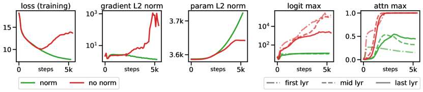
Figure 1: Effect of query/key normalization on an 8B parameter model.

Omitting biases on QKV projections and LayerNorms.

Following PaLM (Chowdhery et al., 2022), the bias terms were removed from the QKV projections and all LayerNorms were applied without bias and centering (Zhang and Sennrich, 2019). This improved accelerator utilization (by 3%), without quality degradation. However, unlike PaLM, we use bias terms for the (in- and out-) MLP dense layers as we have observed improved quality and no speed reduction.

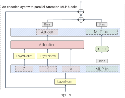
Figure 2: Parallel ViT-22B layer with QK normalization.

Figure 2 illustrates a ViT-22B encoder block. The embedding layer, which includes extracting patches, linear projection, and the addition of position embedding follow those used in the original ViT. We use multi-head attention pooling (Cordonnier et al., 2019; Zhai et al., 2022a) to aggregate the per-token representations in the head.

ViT-22B is uses patch size of $14\times 14$ with images at resolution $224\times 224$ (pre-processed by inception crop followed by random horizontal flip). Similar to the original ViT (Dosovitskiy et al., 2021), ViT-22B employs a learned 1D positional embedding. During fine-tuning on high-resolution images (different number of visual tokens), we perform a 2D interpolation of the pre-trained position embeddings, according to their location in the original image.

Other hyperparameters for the ViT-22B model architecture are presented in Table 1, compared to the previously reported largest ViT models, ViT-G (Zhai et al., 2022a) and ViT-e (Chen et al., 2022).

Table 1: ViT-22B model architecture details.

Name	Width	Depth	MLP	Heads	Params [M]
ViT-G	1664	48	08192	16	1843
ViT-e	1792	56	15360	16	3926
ViT-22B	6144	48	24576	48	21743

Following the template in Mitchell et al. (2019), we provide the model card in LABEL:tab:model_card (Appendix C).

3 Training Infrastructure and Efficiency

ViT-22B is implemented in JAX (Bradbury et al., 2018) using the FLAX library (Heek et al., 2020) and built within Scenic (Dehghani et al., 2022). It leverages both model and data parallelism. In particular, we used the jax.xmap API, which provides explicit control over both the sharding of all intermediates (e.g. weights and activations) as well as inter-chip communication. We organized the chips into a 2D logical mesh of size $t\times k$, where $t$ is the size of the data-parallel axis and $k$ is the size of the model axis. Then, for each of the $t$ groups, $k$ devices get the same batch of images, each device keeps only $1/k$ of the activations and is responsible for computing $1/k$ of the output of all linear layers (detailed below).

(a) The matrix $A$ is row-sharded across the devices.

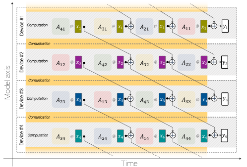
(b) The matrix $A$ is column-sharded across the devices.

Figure 3: Asynchronized parallel linear operation ($y=Ax$): model parallel matrix multiplication with overlapping communication and computation across devices.

Asynchronous parallel linear operations.

As we use explicit sharding, we built a wrapper around the dense layers in FLAX that adapts them to the setting where their inputs are split across $k$ devices. To maximize throughput, two aspects have to be considered — computation and communication. Namely, we want the operations to be analytically equivalent to the unsharded case, to communicate as little as possible, and ideally to have them overlap (Wang et al., 2022a) so that we can keep the matrix multiply unit, where most of the FLOP capacity is, busy at all times.

To illustrate the process, consider the problem of computing $y=Ax$ under the constraint that the $i$-th block of $x$ and $y$ both reside on the $i$-th device. We denote the blocks of $A\in\mathbb{R}^{m\times n}$ by $A_{i,j}\in\mathbb{R}^{\frac{m}{k}\times\frac{n}{k}}$, and analogously $x_{i}\in\mathbb{R}^{\frac{n}{k}}$ and $y_{j}\in\mathbb{R}^{\frac{m}{k}}$, with $i,j\in\{1,\ldots,k\}$. The first option is to have device $i$ hold the $i$-th block of rows, necessary for computation of $y_{i}$, so that to compute $y_{i}$ the chip needs to communicate $k-1$ times to complete $x$, a total of $(k-1)(n/k)$ floats. Alternatively, device $i$ can hold the $i$-th block of columns, all acting on $x_{i}$. This way, the device computes the vectors $y_{ji}=A_{ji}x_{i}$, which have to be communicated (scatter-reduced) with the other devices. Note that here the communicated vectors belong to the output space, a total of $(k-1)(m/k)$ floats. This asymmetry is leveraged in communication costs when $n\neq m$; column-sharding is used in the computation of the output of the MLP in a Transformer, where $n=4m$, and row-sharding elsewhere.

Furthermore, matrix multiplications are overlapped with the communication with the neighbours. This asynchronous approach allows for high matrix core utilization and increased device efficiency, while minimizing waiting on incoming communication. Figure 3 presents the overlapping communication and computation across $4$ devices with the parallel linear operation in row-sharding and column-sharding modes. The general case of this technique is presented in Wang et al. (2022a), who also introduce the XLA operations we leverage here.

Parameter sharding.

The model is data-parallel on the first axis. Each parameter can be either fully replicated over this axis, or have each device hold a chunk of it. We opted to shard some large tensors from the model parameters to be able to fit larger models and batch sizes. This means that the device would have to gather the parameters before computing of the forward and scatter on the backward pass, but again, note that this happens asynchronous with computation. In particular, while computing one layer the device can start communicating the weights of the next one, thus minimizing the communication overhead.

Using these techniques, ViT-22B processes $1.15$k tokens per second per core during training (forward and backward pass) on TPUv4 (Jouppi et al., 2020). ViT-22B’s model flops utilization (MFU) (Chowdhery et al., 2022; Dehghani et al., 2021a) is 54.9%, indicating a very efficient use of the hardware. Note that PaLM reports 46.2% MFU (Chowdhery et al., 2022; Pope et al., 2022) and we measured 44.0% MFU for ViT-e (data-parallel only) on the same hardware.

4 Experiments

4.1 Training details

Dataset.

ViT-22B is trained on a version of JFT (Sun et al., 2017), extended to around 4B images (Zhai et al., 2022a). These images have been semi-automatically annotated with a class-hierarchy of 30k labels. Following the original Vision Transformer, we flatten the hierarchical label structure and use all the assigned labels in a multi-label classification fashion employing the sigmoid cross-entropy loss.

Hyperparameters.

ViT-22B was trained using 256 visual tokens per image, where each token represents a $14\times 14$ patch extracted from $224\times 224$ sized images. ViT-22B is trained for 177k steps with batch size of 65k: approximately 3 epochs. We use a reciprocal square-root learning rate schedule with a peak of $10^{-3}$, and linear warmup (first 10k steps) and cooldown (last 30k steps) phases. For better few-shot adaptation, we use a higher weight decay on the head ($3.0$) than body ($0.03$) for upstream training (Zhai et al., 2022a; Abnar et al., 2021).

4.2 Transfer to image classification

Efficient transfer learning with large scale backbones is often achieved by using them as frozen feature extractors. This section presents the evaluation results of ViT-22B for image classification using linear probing and locked-image tuning as well as out-of-distribution transfer. Additional results for Head2Toe transfer, few-shot transfer, and linear probing with L-BFGS can be found in Table 10.

4.2.1 Linear probing

We explored various ways of training a linear probe, our final setup on ImageNet uses SGD with momentum for 10 epochs at 224px resolution, with mild random cropping and horizontal flipping as the only data augmentations, and no further regularizations.

The results presented in Table 2 show that while the returns are diminishing, there is still a notable improvement at this scale. Furthermore, we show that linear probing of larger models like ViT-22B can approach or exceed performance of full fine-tuning of smaller models with high-resolution, which can be often cheaper or easier to do.

Table 2: Linear evaluation on ImageNet-1k (Deng et al., 2009) with varying scale. All models pre-trained on large datasets. Performances of a few high-resolution fine-tuned models from are provided for reference.

Model	IN	ReaL	INv2	ObjectNet	IN-R	IN-A
224px linear probe (frozen)
B/32	80.18	86.00	69.56	46.03	75.03	31.2
B/16	84.20	88.79	75.07	56.01	82.50	52.67
ALIGN (360px)	85.5	-	-	-	-	-
L/16	86.66	90.05	78.57	63.84	89.92	67.96
g/14	88.51	90.50	81.10	68.84	92.33	77.51
G/14	88.98	90.60	81.32	69.55	91.74	78.79
e/14	89.26	90.74	82.51	71.54	94.33	81.56
22B	89.51	90.94	83.15	74.30	94.27	83.80
High-res fine-tuning
L/16	88.5	90.4	80.4	-	-	-
FixNoisy-L2	88.5	90.9	80.8	-	-	-
ALIGN-L2	88.64	-	-	-	-	-
MaxViT-XL	89.53	-	-	-	-	-
G/14	90.45	90.81	83.33	70.53	-	-
e/14	90.9	91.1	84.3	72.0	-	-

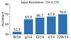
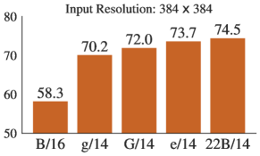
Figure 4: Linear probing on iNaturalist 2017 with different input resolutions. ViT-22B leads to significant accuracy improvement especially when the input size is small.

We further test linear separability on the fine-grained classification dataset, iNaturalist 2017 (Cui et al., 2018). It has 5,089 find-grained categories, belonging to 13 super-categories. Unlike ImageNet, the image numbers in different categories are not balanced. The long-tail distribution of concepts is more challenging for classification. We compare ViT-22B with the other ViT variants. Similar to the linear probing on ImageNet, we use SGD with 0.001 starting learning rate and no weight decay to optimize the models and train for 30 epochs with cosine learning rate schedule with 3 epochs of linear warm-up. We test both $224$px and $384$px input resolutions. Figure 4 shows the results. We observe that ViT-22B significantly improves over the other ViT variants, especially with the standard $224$px input resolution. This suggests the large number of parameters in ViT-22B are useful for extracting detailed information from the images.

4.2.2 Zero-shot via locked-image tuning

Experimental setup.

Following the Locked-image Tuning (LiT) (Zhai et al., 2022b) protocol, we train a text tower contrastively to match the embeddings produced by the frozen ViT-22B model. With this text tower, we can easily perform zero-shot classification and zero-shot retrieval tasks. We train a text Transformer with the same size as ViT-g (Zhai et al., 2022a) on the English subset of the WebLI dataset (Chen et al., 2022) for 1M steps with a 32K batch size. The images are resized to $288$px, and the text is tokenized to 16 tokens using a SentencePiece (Kudo and Richardson, 2018) tokenizer trained on the English C4 dataset.

Results.

Table 3 shows the zero-shot transfer results of ViT-22B against CLIP (Radford et al., 2021), ALIGN (Jia et al., 2021), BASIC (Pham et al., 2021), CoCa (Yu et al., 2022a), LiT (Zhai et al., 2022b) with ViT-g (Zhai et al., 2022a) and ViT-e (Chen et al., 2022) models. The bottom part of Table 3 compares three ViT models using the LiT recipe. On all the ImageNet test sets, ViT-22B achieves either comparable or better results. Notably, zero-shot results on the ObjectNet test set is highly correlated with the ViT model size. The largest ViT-22B sets the new SOTA on the challenging ObjectNet test set. Appendix A shows zero-shot classification examples on OOD images.

Table 3: Zero-shot transfer results on ImageNet (variants).

Model	IN	IN-v2	IN-R	IN-A	ObjNet	ReaL
CLIP	76.2	70.1	88.9	77.2	72.3	-
ALIGN	76.4	70.1	92.2	75.8	72.2	-
BASIC	85.7	80.6	95.7	85.6	78.9	-
CoCa	86.3	80.7	96.5	90.2	82.7	-
LiT-g/14	85.2	79.8	94.9	81.8	82.5	88.6
LiT-e/14	85.4	80.6	96.1	88.0	84.9	88.4
LiT-22B	85.9	80.9	96.0	90.1	87.6	88.6

4.2.3 Out-of-distribution

Experimental setup.

We construct a label-map from JFT to ImageNet, and label-maps from ImageNet to different out-of-distribution datasets, namely ObjectNet (Barbu et al., 2019), ImageNet-v2 (Recht et al., 2019) ImageNet-R (Hendrycks et al., 2020), and ImageNet-A (Hendrycks et al., 2021). ImageNet-R and ImageNet-A use the same 200 label subspace of ImageNet (constructed in such a way that misclassifications would be considered egregious (Hendrycks et al., 2021)), while ObjectNet has 313 categories, of which we only consider the 113 ones overlapping with the ImageNet label space. For ObjectNet and ImageNet-A we do an aspect-preserving crop of the central 75% of the image, for the other datasets we first resize them to a square format and then take a 87.5% central crop. Image input resolution is 224px for pre-trained checkpoints and 384px, 518px, 560px for models fine-tuned on ImageNet.

Results.

We can confirm results from (Taori et al., 2020; Djolonga et al., 2021; Kolesnikov et al., 2020) that scaling the model increases out-of-distribution performance in line with the improvements on ImageNet. This holds true for models that have only seen JFT images, and for models fine-tuned on ImageNet. In both cases, ViT-22B continues the trend of better OOD performance with larger models (Figure 5, Table 11). While fine-tuning boosts accuracy on both ImageNet and out-of-distribution datasets, the effective robustness (Andreassen et al., 2021) decreases (Figure 5). Even though ImageNet accuracy saturates, we see a significant increase on ObjectNet from ViT-e/14 to ViT-22B.

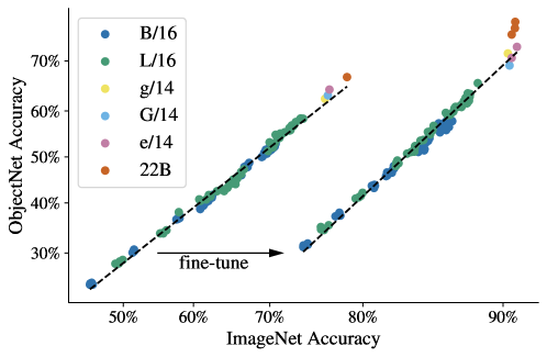
Figure 5: OOD classification performance. Axes are log-scaled as proposed in (Taori et al., 2020). ViT-B and ViT-L are trained on subsets of varying size and varying number of steps on JFT (Zhai et al., 2022a). Fine-tuning boosts both ImageNet and ObjectNet performance, but the increase is more pronounced for in-domain data, which decreases effective robustness (Andreassen et al., 2021), visible as a rightwards shift on the plot. Same data as in Table 11.

4.3 Transfer to dense prediction

Transfer learning for dense prediction is critical especially since obtaining pixel-level labels can be costly. In this section, we investigate the quality of captured geometric and spatial information by the ViT-22B model (trained using image-level classification objective) on semantic segmentation and monocular depth estimation tasks.

4.3.1 Semantic segmentation

Experimental setup.

We evaluate ViT-22B as a backbone in semantic segmentation on three benchmarks: ADE20K (Zhou et al., 2017b), Pascal Context (Mottaghi et al., 2014) and Pascal VOC (Everingham et al., 2010). We analyze the performance in two scenarios: first, using a limited amount of data for transfer; second (in Section E.1), comparing end-to-end fine-tuning versus a frozen backbone with either a linear decoder (Strudel et al., 2021) or UperNet (Xiao et al., 2018). The number of additional parameters ($\approx 1$M for linear and $\approx 783$M for UperNet) is negligible compared to the size of the backbone. We use a fixed resolution ($504$px) and report single scale evaluation.

Results.

We compare ViT-22B to the ViT-L of DeiT-III (Touvron et al., 2022) and ViT-G of Zhai et al. (2022a), when only a fraction of the ADE20k semantic segmentation data is available. We use the linear decoder and end-to-end fine-tuning. From Table 4, we observe that our ViT-22B backbone transfers better when seeing only few segmentation masks. For example, when fine-tuning with only 1200 images (i.e. $1/16$) of ADE20k training data, we reach a performance of 44.7 mIoU, an improvement of $+8.6$ mIoU over DeiT-III Large (Touvron et al., 2022) and $+2.3$ mIoU over ViT-G (Zhai et al., 2022a). When transferring with more data, the performance of ViT-G and ViT-22B converge.

Table 4: Fewshot semantic segmentation on ADE20k, when only a fraction of the training set is used. We report mean IoU for semantic segmentation on the validation set. Transfer is done with end-to-end fine-tuning and a linear decoder, following Strudel et al. (2021). We average over 3 runs.

Fraction of ADE20k train data	$1/16$	$1/8$	$1/4$	$1/2$	$1$
ViT-L (Touvron et al., 2022)	36.1	41.3	45.6	48.4	51.9
ViT-G (Zhai et al., 2022a)	42.4	47.0	50.2	52.4	55.6
ViT-22B (Ours)	44.7	47.2	50.6	52.5	54.9

4.3.2 Monocular depth estimation

Experimental setup.

We largely mirror the set-up explored in Ranftl et al. (2021) and train their Dense Prediction Transformer (DPT) on top of frozen ViT-22B backbone features obtained from the Waymo Open real-world driving dataset (Sun et al., 2020). Here we use only a single feature map (of the last layer) to better manage the high-dimensional ViT features. We also explore a much simpler “linear” decoder as a lightweight readout. In both cases we predict $\log(1+\text{depth})$ obtained from sparse LiDAR as the target and use Mean Squared Error (MSE) as the decoder training loss. We quantify performance using standard depth estimation metrics from the literature (Hermann et al., 2020; Eigen et al., 2014) and also report MSE. We use a resolution of $224\times 224$. Remaining details are deferred to Section E.2.

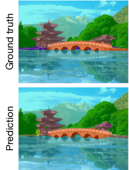
(a) Semantic segmentation

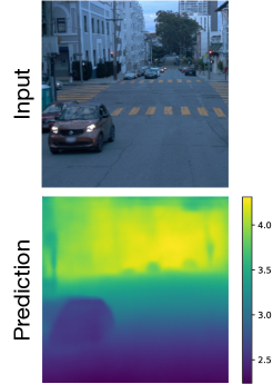
(b) Depth estimation

Figure 6: Dense prediction from frozen ViT-22B features.

Table 5: Monocular depth estimation from frozen ViT features using different decoders on the Waymo Open dataset.

				$\delta$ $\uparrow$
	Model	MSE $\downarrow$	AbsRel $\downarrow$	$<1.1$	$<1.25$	$<1.25^{2}$
DPT	ViT-L	0.027	0.121	0.594	0.871	0.972
	ViT-e	0.024	0.112	0.631	0.888	0.975
	ViT-22B	0.021	0.095	0.702	0.909	0.979
Linear	ViT-L	0.060	0.222	0.304	0.652	0.926
	ViT-e	0.053	0.204	0.332	0.687	0.938
	ViT-22B	0.039	0.166	0.412	0.779	0.960

Results.

Table 5 summarizes our main findings. From the top rows (DPT decoder), we observe that using ViT-22B features yields the best performance (across all metrics) compared to different backbones. By comparing the ViT-22B backbone to ViT-e (a smaller model but trained on the same data as ViT-22B) we find that scaling the architecture improves performance. Further, comparing the ViT-e backbone to ViT-L (a similar architecture to ViT-e but trained on less data) we find that these improvements also come from scaling the pre-training data. These findings demonstrate that both the greater model size and the greater dataset size contribute substantially to the improved performance. Using the linear decoder, it can be observed again that using ViT-22B features yields the best performance. The gap between DPT and linear decoding suggests that while enough geometric information is retained in the ViT features, only some of it is available for a trivial readout. We report qualitative results in Figure 6 and Figures 13 and 14 in Section E.2.

4.4 Transfer to video classification

Experimental setup.

We evaluate the quality of the representations learned by ViT-22B by adapting the model pretrained on images for video classification. We follow the “factorised encoder” architecture of Arnab et al. (2021): Our video model consists of an initial “spatial transformer”, which encodes each frame of the video independently of each other. Thereafter, the representation from each frame is pooled into a single token, which is then fed to a subsequent “temporal transformer” that models the temporal relations between the representations of each frame.

Here, we initialize the “spatial transformer” with the pretrained weights from ViT-22B and freeze them, as this represents a computationally efficient method of adapting large-scale models for video, and also because it allows us to effectively evaluate the representations learned by pretraining ViT-22B. Exhaustive experimental details are included in Appendix F. The temporal transformer is lightweight both in terms of parameters (only 63.7M parameters compared to the 22B frozen parameters in the spatial transformer), and FLOPs as it operates on a single token per frame.

Results.

Table 6: Video classification results. We evaluate the ViT-22B representations by freezing the backbone, and training a small transformer to aggregate frozen, per-frame representations. ViT-22B outperforms the largest previous vision backbone, ViT-e (Chen et al., 2022) which contains 4 billion parameters and is also pretrained on JFT.

	Kinetics 400	Moments in Time
Frozen backbone
CoCA∗	88.0	47.4
ViT-e	86.5	43.6
ViT-22B	88.0	44.9
Fully finetuned SOTA	91.1	49.0

^∗Note that CoCA uses pre-pool spatial features and higher spatial resolution for both datasets. More details in Appendix F.

Table 6 presents our results on video classification on the Kinetics 400 (Kay et al., 2017) and Moments in Time (Monfort et al., 2019) datasets, showing that we can achieve competitive results with a frozen backbone. We first compare to ViT-e (Chen et al., 2022), which has the largest previous vision backbone model consisting of 4 billion parameters, and was also trained on the JFT dataset. We observe that our larger ViT-22B model improves by 1.5 points on Kinetics 400, and 1.3 points on Moments in Time. Our results with a frozen backbone are also competitive with CoCA (Yu et al., 2022a), which performs a combination of contrastive and generative caption pretraining in comparison to our supervised pretraining, and uses many tokens per frame (vs. a single one produced by the pretrained frozen pooling) as well as a higher testing resolution.

Finally, we note that there is headroom for further improvement by full end-to-end fine-tuning. This is evidenced by the current state-of-the-art on Kinetics 400 (Wang et al., 2022b) and Moments in Time (Yu et al., 2022a) which leverage a combination of large-scale video pretraining and full end-to-end fine-tuning on the target dataset.

4.5 Beyond accuracy on downstream tasks

When studying the impact of scaling, there are important aspects to consider beyond downstream task performance. In this section, we probe ViT-22B’s fairness, alignment with human perception, robustness, reliability, and calibration. We find that favorable characteristics emerge when increasing model size. Additional analysis on perceptual similarity and feature attribution can be found in Appendix K and Appendix L.

4.5.1 Fairness

Machine learning models are susceptible to unintended bias. For example, they can amplify spurious correlations in the training data (Hendricks et al., 2018; Caliskan et al., 2017; Zhao et al., 2017; Wang et al., 2020) and result in error disparities (Zhao et al., 2017; Buolamwini and Gebru, 2018; Deuschel et al., 2020). Here, we identify how scaling the model size can help mitigate such issues, by evaluating the bias of ViT-22B and ViT-{L, g, G, e}  (Zhai et al., 2022a; Chen et al., 2022) using demographic parity (DP) as a measure of fairness (Dwork et al., 2012; Zafar et al., 2017).

Figure 7: top: Accuracy (ACC) for ViT variants after debiasing for each DP level. middle: Accuracy for each subgroup in CelebA prior to debiasing. bottom: $y$-axis is absolute difference in performance across the two subgroups: females and males. ViT-22B provides a more equitable performance, compared to smaller ViT architectures.

Experimental Setup.

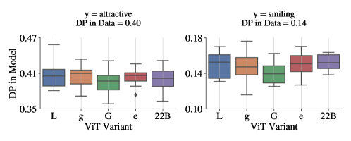
Figure 15: DP in the model often reflects DP in the data in the absence of bias mitigation. In this figure, binary sex is the sensitive attribute and linear heads are trained to predict other attributes in CelebA using pretrained features.

We use CelebA (Liu et al., 2015) with binary gender as a sensitive attribute while the target is “attractive” or “smiling”. We emphasize that such experiments are carried out only to verify technical claims and shall by no means be interpreted as an endorsement of such vision-related tasks. We choose the latter attributes because they exhibit gender related bias as shown in Figure 15.

We train a logistic regression classifier on top of the ViT-22B pretrained features for a total of $50$ epochs and batch size $256$, with a learning rate schedule of $0.01$ (first 25 epochs) and 0.001 (last 25 epochs). After that, we debias using the randomized threshold optimizer (RTO) algorithm of Alabdulmohsin and Lucic (2021), which was shown to be near-optimal and competitive with in-processing methods.

Results.

We observe that scale by itself does not impact DP, c.f. Figure 15. This is perhaps not surprising, as the model is trained to reconstruct a chosen target so the level of DP in accurate models is similar to that of the data itself.

However, scaling to ViT-22B offers benefits for fairness in other aspects. First, scale offers a more favorable tradeoff — performance improves with scale subject to any prescribed level of bias constraint. This is consistent with earlier observations reported in the literature (Alabdulmohsin and Lucic, 2021). Second, all subgroups tend to benefit from the improvement in scale. Third, ViT-22B reduces disparities in performance across subgroups. Figure 7 summarizes results for classification accuracy and Appendix G for expected calibration error (ECE) (Naeini et al., 2015; Guo et al., 2017) and OC-AUC (Kivlichan et al., 2021).

4.5.2 Human Alignment

How well do ViT-22B classification decisions align with human classification decisions? Using the model-vs-human toolbox (Geirhos et al., 2021), we evaluate three ViT-22B models fine-tuned on ImageNet with different resolutions (224, 384, 560). Accross all toolbox metrics, ViT-22B is SOTA: ViT-22B-224 for highest OOD robustness (Figure 19(a)), ViT-22B-384 for the closest alignment with human classification accuracies (Figure 19(b)), and ViT-22B-560 for the largest error consistency (i.e. most human-like error patterns, Figure 19(d)). The ViT-22B models have the highest ever recorded shape bias in vision models: while most models have a strong texture bias (approx. 20–30% shape bias / 70–80% texture bias) (Geirhos et al., 2019); humans are at 96% shape / 4% texture bias and ViT-22B-384 achieves a previously unseen 87% shape bias / 13% texture bias (Figure 8). Overall, ViT-22B measurably improves alignment to human visual object recognition.

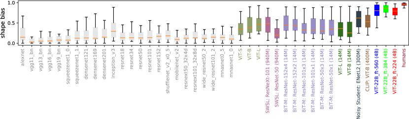
Figure 8: Shape bias: many vision models have a low shape / high texture bias, whereas ViT-22B fine-tuned on ImageNet (red, green, blue trained on 4B images as indicated by brackets after model names, unless trained on ImageNet only) have the highest shape bias recorded in a ML model to date, bringing them closer towards a human-like shape bias.

4.5.3 Plex - pretrained large model extensions

Tran et al. (2022) comprehensively evaluate the reliability of models through the lens of uncertainty, robustnes (see Section 4.2.3) and adaptation (see Section 4.2.2). We focus here on the first aspect of that benchmark. To this end, we consider (1) the OOD robustness under covariate shift with ImageNet-C (Hendrycks and Dietterich, 2019), which we evaluate not only with the accuracy but also uncertainty metrics measuring the calibration (NLL, ECE) and the selective prediction (El-Yaniv and Wiener, 2010) (OC-AUC, see Section 4.5.1), and (2) open-set recognition—also known as OOD detection (Fort et al., 2021), which we evaluate via the AUROC and AUPRC, with Places365 as the OOD dataset (Hendrycks et al., 2019); for more details, see Appendix I.

In Table 7, we report the performance of ViT-L and ViT-22B (both with resolution 384) fine-tuned on ImageNet. To put in perspective the strong gains of ViT-22B, we also show Plex-L, a ViT-L equipped with the two components advocated by Tran et al. (2022), viz, efficient-ensemble (Wen et al., 2019) and heteroscedastic layers (Collier et al., 2021). We discuss the challenges and the results of the usage of those components at the 22B scale (Plex-22B) in Appendix I.

Table 7: ViT-22B evaluated on some representative metrics from the Plex reliability benchmark (Tran et al., 2022)^∗.

		IN-C (mean over shifts)					IN vs. Places365
Metrics		ACC $\uparrow$	NLL $\downarrow$	ECE $\downarrow$	OC-AUC $\uparrow$		AUROC $\uparrow$	AUPRC $\uparrow$
ViT-L/32∗		70.1	1.28	0.05	0.91		0.83	0.96
Plex-L/32∗		71.3	1.21	0.02	0.91		0.83	0.97
ViT-22B		83.7	0.63	0.01	0.97		0.88	0.98

4.5.4 Calibration

Along with the robustness of Section 4.2.3, it is also natural to wonder how the calibration property of ViT evolves as the scale increases. To this end, we focus on the study of Minderer et al. (2021) that we extend with ViT-22B.

In Figure 9, we consider ViT-22B fine-tuned on ImageNet (resolution 384) and report the error (i.e., one minus accuracy) versus the calibration, as measured by the expected calibration error (ECE) (Naeini et al., 2015; Guo et al., 2017). We see how ViT-22B remarkably improves the tradeoff between accuracy and calibration. The conclusion holds both without (left) and with (right) a temperature-scaling of the logits that was observed to better capture the calibration trends across model families (Minderer et al., 2021). More details can be found in Appendix H.

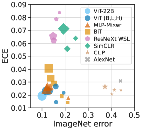
(a) Unscaled

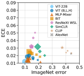
(b) Temperature-scaled

Figure 9: ViT-22B (light-blue circle) improves the Pareto frontier of the accuracy vs. the calibration (ECE). Left/right panels are without/with temperature scaling, respectively.

4.5.5 Distillation

We perform model distillation (Hinton et al., 2015) to compress the ViT-22B into smaller, more widely usable ViTs. We distill ViT-22B into ViT-B/16 and ViT-L/16 by following the procedure of Beyer et al. (2022b). Using ImageNet-finetuned (at 384px) ViT-22B, we annotated 500 random augmentations and mixup transforms of each ImageNet image with ViT-22B logits. Then, we minimize the KL divergence between the student and the teacher predictive distributions. We train for 1000 epochs after initializing the student architecture from checkpoints pre-trained on JFT. The results are shown in Table 8, and we see that we achieve new SOTA on both the ViT-B and ViT-L sizes.

Table 8: Distillation results, finetuned at 384 resolution.

Model		ImageNet1k
ViT-B/16	(Dosovitskiy et al., 2021) (JFT ckpt.)	84.2
	(Zhai et al., 2022a) (JFT ckpt.)	86.6
	(Touvron et al., 2022) (INet21k ckpt.)	86.7
	Distilled from ViT-22B (JFT ckpt.)	88.6
ViT-L/16	(Dosovitskiy et al., 2021) (JFT ckpt.)	87.1
	(Zhai et al., 2022a) (JFT ckpt.)	88.5
	(Touvron et al., 2022) (INet21k ckpt.)	87.7
	Distilled from ViT-22B (JFT ckpt.)	89.6

5 Conclusion

We presented ViT-22B, the currently largest vision transformer model at 22 billion parameters. We show that with small, but critical changes to the original architecture, we can achieve both excellent hardware utilization and training stability, yielding a model that advances the SOTA on several benchmarks. In particular, great performance can be achieved using the frozen model to produce embeddings, and then training thin layers on top. Our evaluations further show that ViT-22B is more aligned with humans when it comes to shape and texture bias, and offers benefits in fairness and robustness, when compared to existing models.

Appendix A Zero-shot Classification Examples

Figure 10 contains example zero-shot classifications of generated images. These images were provided by the Parti (Yu et al., 2022b) and Imagen (Saharia et al., 2022) models. The training data for the ViT-22B vision backbone and the LiT text backbone was created before these models were trained, therefore these images are not present in the training data. Further, the objects and scenes contained in these images are highly out-of-distribution relative to the distribution of natural images on the web.

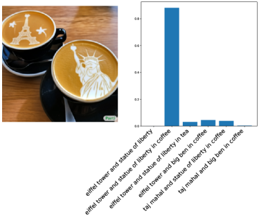
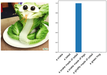
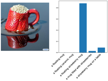
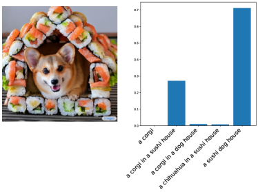
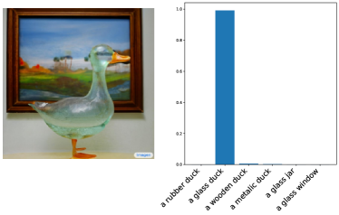
Figure 10: Examples of zero-shot classification results on images generated by the Parti (Yu et al., 2022b) and Imagen (Saharia et al., 2022) models. These examples contain unusual objects/scenes that do not occur in the training distribution.

Appendix B Scalability

When scaling up the default ViT architecture, we encountered training instability in ViT at Adam $1e^{-3}$. Initially, the loss would decrease as normal, but within 2000 steps the loss steadily increased. Figure 1 shows the behavior of attention logits during training for an 8B parameter model. Without normalization, attention logits quickly grow to over $50000$ in magnitude, resulting in one-hot attention weights after the softmax, and subsequently unstable training losses and gradients.

To avoid instability, the learning rate of ViT was originally reduced with increasing model scale, from 1e-3 down to 4e-4 for ViT-H (Dosovitskiy et al., 2021). We retrain models up to ViT-L, comparing models trained similar to ViT, to models which have the normalization/reduced precision. For the latter, the learning rate is kept at 1e-3 and not reduced for larger models. With the QK-normalization, the higher 1e-3 learning rate remains stable. The results, shown in Figure 11, demonstrate increasing benefits with scale, likely due to enabling the larger learning rate.

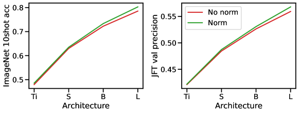
Figure 11: Training models with and without query/key normalization; those that do not have normalization are trained with lower learning rates at larger scale, whereas those with normalization have a consistent learning rate of 1e-3.

Appendix C Model Card

LABEL:tab:model_card presents the model card (Mitchell et al., 2019) of the ViT-22B model.

Table 9: Model Card of ViT-22B model.

Model Summary
Model Architecture	Dense encoder-only model with 22 billion parameters. Transformer model architecture with variants to speed up and stabilize the training. For details, see Model Architecture (Section 2).
Input(s)	The model takes images as input.
Output(s)	The model generates a class label as output during pretraining.
Usage
Application	The primary use is research on computer vision applications as a feature extractor that can be used in image recognition (finetuning, fewshot, linear-probing, zeroshot), dense prediction (semantic segmentation, depth estimation), video action recognition and so on. On top of that, ViT-22B is used in research that aim at understanding the impact of scaling vision transformers.
Known Caveats	When using ViT-22B, similar to any large scale model, it is difficult to understand how the model arrived at a specific decision, which could lead to lack of trust and accountability. Moreover, we demonstrated that ViT-22B is less prone to unintentional bias and enhances current vision backbones by reducing spurious correlations. However, this was done through limited studies and particular benchmarks. Besides, there is always a risk of misuse in harmful or deceitful contexts when it comes to large scale machine learning models. ViT-22B should not be used for downstream applications without a prior assessment and mitigation of the safety and fairness concerns specific to the downstream application. We recommend spending enough time and energy on mitigation the risk at the downstream application level.
System Type
System Description	This is a standalone model.
Upstream Dependencies	None.
Downstream Dependencies	None.
Implementation Frameworks
Hardware & Software: Training	Hardware: TPU v4 (Jouppi et al., 2020). Software: JAX (Bradbury et al., 2018), Flax (Heek et al., 2020), Scenic (Dehghani et al., 2022).
Hardware & Software: Deployment	Hardware: TPU v4 (Jouppi et al., 2020). Software: Scenic (Dehghani et al., 2022).
Compute Requirements	ViT-22B was trained on 1024 TPU V4 chips for 177K steps.
Model Characteristics
Model Initialization	The model is trained from a random initialization.
Model Status	This is a static model trained on an offline dataset.
Model Stats	ViT-22B model has 22 billion parameters.
Data Overview
Training Dataset	ViT-22B is trained on a version of JFT (Sun et al., 2017), extended to contain around 4B images (Zhai et al., 2022a). See Section 4.1 for the description of datasets used to train ViT-22B.
Evaluation Dataset	We evaluate the ViT-22B on a wide variety of tasks and report the results on each individual tasks and datasets (Dehghani et al., 2021b). Specifically, we evaluate the models on: ADE20K (Zhou et al., 2017b), Berkeley Adobe Perceptual Patch Similarity (BAPPS) (Zhang et al., 2018), Birds (Wah et al., 2011), Caltech101 (Li et al., 2022), Cars (Krause et al., 2013), CelebA (Liu et al., 2015), Cifar-10 (Krizhevsky et al., 2009), Cifar-100 (Krizhevsky et al., 2009), CLEVR/count (Johnson et al., 2017), CLEVR/distance (Johnson et al., 2017), ColHist (Kather et al., 2016), DMLab  (Beattie et al., 2016), dSprites/location (Matthey et al., 2017), dSprites/orientation (Matthey et al., 2017), DTD (Cimpoi et al., 2014), EuroSAT (Helber et al., 2019), Flowers102 (Nilsback and Zisserman, 2008), ImageNet (Deng et al., 2009), Inaturalist (Cui et al., 2018), ImageNet-v2 (Recht et al., 2019), ImageNet-R (Hendrycks et al., 2020), ImageNet-A (Hendrycks et al., 2021), ImageNet-C (Hendrycks and Dietterich, 2019), ImageNet-ReaL-H (Tran et al., 2022), Kinetics 400 (Kay et al., 2017), KITTI (Geiger et al., 2013), Moments in Time (Monfort et al., 2019), ObjectNet (Barbu et al., 2019), Pascal Context (Mottaghi et al., 2014), Pascal VOC (Everingham et al., 2010), Patch Camelyon (Teh and Taylor, 2019), Pets (Parkhi et al., 2012), Places365 (Zhou et al., 2017a), Resisc45 (Cheng et al., 2017), Retinopathy  (Kaggle and EyePacs, 2015), SmallNORB/azimuth (LeCun et al., 2004), SmallNORB/elevation (LeCun et al., 2004), Sun397 (Xiao et al., 2010), SVHN (Netzer et al., 2011), UC Merced (Yang and Newsam, 2010), Waymo Open real-world driving dataset (Sun et al., 2020).
Evaluation Results
Benchmark Information	• Quality of transfer to downstream tasks. – Transfer to image classification (via linear probing, zero-shot transfer, OOD transfer, fewshot transfer, Head2Toe transfer, and fine-tuning). * Datasets Used: Birds (Wah et al., 2011), Caltech101 (Li et al., 2022), Cars (Krause et al., 2013), CelebA (Liu et al., 2015), Cifar-10 (Krizhevsky et al., 2009), Cifar-100 (Krizhevsky et al., 2009), CLEVR/count (Johnson et al., 2017), CLEVR/distance (Johnson et al., 2017), ColHist (Kather et al., 2016), DMLab  (Beattie et al., 2016), dSprites/location (Matthey et al., 2017), dSprites/orientation (Matthey et al., 2017), DTD (Cimpoi et al., 2014), EuroSAT (Helber et al., 2019), Flowers102 (Nilsback and Zisserman, 2008), ImageNet (Deng et al., 2009), iNaturalist (Cui et al., 2018), ImageNet-v2 (Recht et al., 2019), ImageNet-R (Hendrycks et al., 2020), ImageNet-A (Hendrycks et al., 2021), ImageNet-C (Hendrycks and Dietterich, 2019), ImageNet-ReaL-H (Tran et al., 2022), Kinetics 400 (Kay et al., 2017), KITTI (Geiger et al., 2013), ObjectNet (Barbu et al., 2019), Patch Camelyon (Teh and Taylor, 2019), Pets (Parkhi et al., 2012), Places365 (Zhou et al., 2017a), Resisc45 (Cheng et al., 2017), Retinopathy  (Kaggle and EyePacs, 2015), SmallNORB/azimuth (LeCun et al., 2004), SmallNORB/elevation (LeCun et al., 2004), Sun397 (Xiao et al., 2010), SVHN (Netzer et al., 2011), UC Merced (Yang and Newsam, 2010). – Transfer to video classification. * Datasets Used: Kinetics 400 (Kay et al., 2017), Moments in Time (Monfort et al., 2019). – Transfer to dense prediction. * Semantic segmentation · Datasets Used: ADE20k (Zhou et al., 2017b), Pascal Context (Mottaghi et al., 2014), Pascal VOC (Everingham et al., 2010). * Depth estimation · Dataset used: Waymo Open real-world driving dataset (Sun et al., 2020). • Quality of learned features. – Fairness. * Dataset used: CelebA (Liu et al., 2015). – Human alignment. * We used the model-vs-human toolbox (Geirhos et al., 2021). – Calibration. * We follow the setup of Minderer et al. (2021). We use ImageNet validation set (Deng et al., 2009). – Perceptual similarity. * Dataset used: Berkeley Adobe Perceptual Patch Similarity (BAPPS) dataset (Zhang et al., 2018) – Feature attribution. * Dataset used: ImageNet (Deng et al., 2009).
Evaluation Results	All results are reported in  Section 4.
Model Usage & Limitations
Sensitive Use	ViT-22B should not be used for any unacceptable vision model use cases. For example: for detecting demographic human features for non-ethical purposes, as a feature extractor used to condition on and generate toxic content, or for captcha-breaking. We also do not approve use of ViT-22B in applications like surveillance, law enforcement, healthcare, or hiring and employment, and self-driving cars without putting measures in place to mitigate the ethical risks.
Known Limitations	ViT-22B is designed for research. The model has not been tested in settings outside of research that can affect performance, and it should not be used for downstream applications without further analysis on factors in the proposed downstream application.
Ethical Considerations & Risks	In order to train ViT-22B, we conducted an analysis of sensitive category associations on the JFT-4B dataset as described in Aka et al. (2021). This process involved measuring the per label distribution of sensitive categories across the raw data, cleaned data, and models trained on this data, as well as labels verified by human raters. To further enhance the data quality, human raters also assisted in removing offensive content from the dataset. Our analysis using standard fairness benchmarks shows that ViT-22B increases performance for all subgroups while minimizing disparities among them. However, it is important to note that there may be situations where utilizing ViT-22B could pose ethical concerns. Therefore, we recommend conducting custom ethical evaluations for any new applications of ViT-22B.

Appendix D Transfer to image classification: More results and addition details

D.1 Linear probing with L-BFGS

An alternative to doing linear probing with SGD is to use the convex optimization technique, L-BFGS (Byrd et al., 1995). It is very effective and has strict convergence guarantees. We compare SGD and L-BFGS for a variety of ViT models using the ImageNet-1k datasset. Specifically, we precompute image embeddings by resizing input images to 224px resolution and then solve the multiclass logistic regression problem with L-BFGS. We also sweep the L2 regularization parameter and select the optimal one using 20000 holdout images from the training data (approximately 2% of the training data). In Table 10 we compare the resulting model with the SGD baseline from the main text. It demonstrates that L-BFGS matches or lags behind SGD approach, so we selected the latter technique for our core experiments.

Table 10: Comparison of SGD and L-BFGS for linear probing on ImageNet-1k. The numbers indicate top-1 accuracy.

Linear Probing	B/32	B/16	L/16	g/14	G/14	e/14	22B
L-BFGS	79.94	84.06	86.64	88.46	88.79	89.08	89.27
SGD	80.18	84.20	86.66	88.51	88.98	89.26	89.51

D.2 Out of distribution classification

Table 11: OOD Classification. Results from models fine-tuned on ImageNet (top half), and models that were only trained on JFT and evaluated with a label-map (bottom half). Models with “ema” are fine-tuned with Polyak averaging, similar to (Dosovitskiy et al., 2021). B/16, L/16, g/14, and G/14 are from (Zhai et al., 2022a), and e/14 is from (Chen et al., 2022). IN^† uses same resize without crop like in the original publication. See Figure 5 and Section 4.2.3 for discussion of the results, and details about datasets and pre-processing.

Model	Fine-tuned	IN	IN†	INv2	ObjectNet	IN-R	IN-A
e/14 ema	560px	90.70	90.84	84.38	72.53	94.49	88.44
22B ema	560px	90.62	-	84.65	76.70	95.05	89.12
22B	560px	90.60	-	84.38	75.69	94.62	88.55
22B	384px	90.44	-	84.28	74.64	94.44	87.95
e/14 ema	384px	90.44	-	83.95	70.56	93.56	87.16
G/14 ema	518px	90.33	90.47	83.53	69.14	94.22	86.95
g/14 ema	518px	90.25	90.11	83.61	71.36	93.37	86.12
L/16	384px	88.60	-	80.74	65.73	90.32	78.65
B/16	384px	87.02	-	78.21	57.83	82.91	66.08
22B	-	78.5	-	72.5	66.9	91.6	79.9
e/14	-	76.7	-	71.0	64.4	90.6	75.3
G/14	-	76.6	-	70.9	63.3	90.2	75.1
g/14	-	76.3	-	70.5	62.6	89.8	73.7
L/16	-	73.9	-	66.9	58.4	86.8	64.6
B/16	-	70.7	-	62.9	52.9	81.4	51.1

D.3 Head2Toe

The cost of fine-tuning a model during transfer learning goes up with increased model size and often requires the same level of resources as training the model itself. Linear probing on the other hand is much cheaper to run, however it often performs worse than fine-tuning. Recent work showed that training a linear classifier on top of the intermediate features can provide significant gains compared to using the last-layer only, especially for target tasks that are significantly different from the original pre-training task (Evci et al., 2022; Adler et al., 2020; Khalifa et al., 2022).

In Table 12 we compare Head2Toe (Evci et al., 2022) with Linear probe on common vision benchmarks and VTAB-1k (Zhai et al., 2019). We include Finetuning results as a comparison point. We use a simplified version of Head2Toe with no feature selection. Experimental details are shared below. Head2Toe achieves 7% better results on VTAB-1k, however fails to match the full finetuning performance (-6%). On other benchmarks (CIFARs, Flowers and Pets), all methods perform similarly potentially. Head2Toe improves over Linear only for the Cifar-100 task. For the remaining tasks it either achieves the same performance or worse (Pets).

All experiments presented here use images with the default resolution of 224. Head2Toe uses the following intermediate features: (1) output of each of the 48 blocks, (2) features after the positional embedding, (3) features after the pooling head (4) pre-logits and logits. We average each of these features among the token dimension and concatenate them; resulting in a 349081 dimensional feature vector. In contrast, linear probe uses the 6144 dimensional prelogit features, which makes Head2Toe training roughly 50 times more expensive. However, given the extraordinary size of the original model, Head2Toe requires significantly less FLOPs and memory compared to fine-tuning. For all tasks (4 standard and 19 VTAB-1k), we search over 2 learning rates (0.01, 0.001) and 2 training lengths (500 and 10000 (2500 for VTAB-1k) steps) using the validation set.

Table 12: Frozen evaluation using linear and Head2Toe (H2T) probe on the VTAB-1k benchmark and four other image classification tasks. We report mean accuracies averaged using 3 seeds.

Method	VTAB-Average	Natural	Specialized	Structured	CIFAR-10	CIFAR-100	Flowers	Pets
Finetuning	76.71	89.09	87.08	61.83	99.63	95.96	97.59	99.75
Linear	63.15	80.86	87.05	35.70	99.37	93.39	99.75	98.15
H2T	70.12	84.60	88.61	48.19	99.45	94.11	99.69	97.46

D.4 Few-shot

We replicate the experimental setup of  (Abnar et al., 2021) to evaluate the ViT-22B model and baselines on 25 tasks (Table 13) using few-shot transfer setups. The results of few-shot transfer of different models using 1, 5, 10, and 25 shots are presented in Figure 12. Scaling up can improve performance in many tasks, but in some cases, downstream accuracy does not improve with increased scale. This may be due to the higher dimension of the representation from the ViT-22B model, which may require more regularization as the size of the head grows to prevent overfitting. Further study is needed to investigate this.

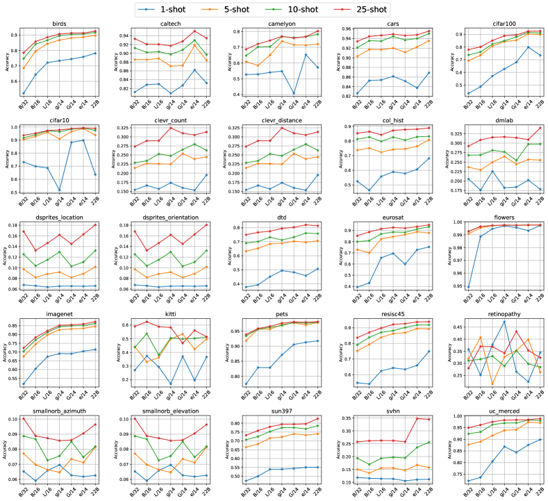
Figure 12: Few-shot transfer with 1, 5, 10, and 25 shots on 25 vision tasks (Abnar et al., 2021).

Table 13: Summary of datasets used in our few-shot experiments in Figure 12

Dataset	Description	Reference
ImageNet	1.28M labelled natural images.	(Deng et al., 2009)
Caltech101	The task consists in classifying pictures of objects (101 classes plus a background clutter class), including animals, airplanes, chairs, or scissors. The image size varies, but it typically ranges from 200-300 pixels per edge.	(Li et al., 2022)
CIFAR-10	The task consists in classifying natural images (10 classes, with 6000 training images each). Some examples include apples, bottles, dinosaurs, and bicycles. The image size is 32x32.	https://www.cs.toronto.edu/~kriz/cifar.html
CIFAR-100	The task consists in classifying natural images (100 classes, with 500 training images each). Some examples include apples, bottles, dinosaurs, and bicycles. The image size is 32x32.	https://www.cs.toronto.edu/~kriz/cifar.html
DTD	The task consists in classifying images of textural patterns (47 classes, with 120 training images each). Some of the textures are banded, bubbly, meshed, lined, or porous. The image size ranges between 300x300 and 640x640 pixels.	(Cimpoi et al., 2014)
Pets	The task consists in classifying pictures of cat and dog breeds (37 classes with around 200 images each), including Persian cat, Chihuahua dog, English Setter dog, or Bengal cat. Images dimensions are typically 200 pixels or larger.	https://www.robots.ox.ac.uk/~vgg/data/pets/
Sun397	The Sun397 task is a scenery benchmark with 397 classes and, at least, 100 images per class. Classes have a hierarchy structure and include cathedral, staircase, shelter, river, or archipelago. The images are (colour) 200x200 pixels or larger.	https://vision.princeton.edu/projects/2010/SUN/
Flowers102	The task consists in classifying images of flowers present in the UK (102 classes, with between 40 and 248 training images per class). Azalea, Californian Poppy, Sunflower, or Petunia are some examples. Each image dimension has at least 500 pixels.	https://www.robots.ox.ac.uk/~vgg/data/flowers/102/
SVHN	This task consists in classifying images of Google’s street-view house numbers (10 classes, with more than 1000 training images each). The image size is 32x32 pixels.	http://ufldl.stanford.edu/housenumbers/
CLEVR/count	CLEVR is a visual question and answer dataset designed to evaluate algorithmic visual reasoning. We use just the images from this dataset, and create a synthetic task by setting the label equal to the number of objects in the images.	(Johnson et al., 2017)
CLEVR/distance	Another synthetic task we create from CLEVR consists of predicting the depth of the closest object in the image from the camera. The depths are bucketed into size bins.	(Johnson et al., 2017)
Retinopathy	The Diabetic Retinopathy dataset consists of image-label pairs with high-resolution retina images, and labels that indicate the presence of Diabetic Retinopathy (DR) in a 0-4 scale (No DR, Mild, Moderate, Severe, or Proliferative DR).	https://www.kaggle.com/c/diabetic-retinopathy-detection/data
Birds	Image dataset with photos of 200 bird species (mostly North American).	(Wah et al., 2011)
Patch Camelyon	The Patch Camelyon dataset contains 327,680 images of histopathologic scans of lymph node sections. The classification task consists in predicting the presence of metastatic tissue in given image (i.e., two classes). All images are 96x96 pixels.	(Teh and Taylor, 2019)
Resisc45	The Remote Sensing Image Scene Classification (RESISC) dataset is a scene classification task from remote sensing images. There are 45 classes, containing 700 images each, including tennis court, ship, island, lake, parking lot, sparse residential, or stadium. The image size is RGB 256x256 pixels.	(Cheng et al., 2017)
EuroSAT	The task consists in classifying Sentinel-2 satellite images into 10 different types of land use (Residential, Industrial, River, Highway, etc). The spatial resolution corresponds to 10 meters per pixel, and the image size is 64x64 pixels.	(Helber et al., 2019)
dSprites/location	The dSprites dataset was originally designed to assess disentanglement properties of unsupervised learning algorithms. In particular, each image is a 2D shape where six factors are controlled: color, shape, scale, rotation, and (x,y) center coordinates. Images have 64x64 black-and-white pixels. This task consists in predicting the x (horizontal) coordinate of the object. The locations are bucketed into 16 bins	https://github.com/deepmind/dsprites-dataset/
dSprites/orientation	We create another task from dSprites consisting in predicting the orientation of each object, bucketed into 16 bins.	https://github.com/deepmind/dsprites-dataset/https://github.com/deepmind/dsprites-dataset/
SmallNORB/azimuth	The Small NORB dataset contains images of 3D-toys from 50 classes, including animals, human figures, airplanes, trucks, and cars. The image size is 640x480 pixels. In this case, we define labels depending on the azimuth (angle of horizontal deviation), in intervals of 20 degrees (18 classes).	(LeCun et al., 2004)
SmallNORB/elevation	Another synthetic task we create from Small NORB consists in predicting the elevation in the image. There are 9 classes, corresponding to 9 different elevations ranging from 30 to 70 degrees, in intervals of 5 degrees	(LeCun et al., 2004)
DMLab	The DMLab (DeepMind Lab) is a set of control environments focused on 3D navigation and puzzle-solving tasks. The Dmlab dataset contains frames observed by the agent acting in the DeepMind Lab environment, which are annotated by the distance between the agent and various objects present in the environment. The goal is to evaluate the ability of a visual model to reason about distances from the visual input in 3D environments. The Dmlab dataset consists of 360x480 color images in 6 classes. The classes are close, far, very far × positive reward, negative reward respectively.	(Beattie et al., 2016)
KITTI	The KITTI task consists in predicting the (binned) depth to the vehicle (car, van, or truck) in the image. There are 4 bins / classes.	(Geiger et al., 2013)
ColHist	Classification of textures in colorectal cancer histology. Each example is a 150 x 150 x 3 RGB image of one of 8 classes.	https://www.tensorflow.org/datasets/catalog/colorectal_histology
UC Merced	21 class land use image dataset	https://usdahsi.ucmerced.edudatasets/landuse.html
Cars	The Cars dataset contains 16,185 images of 196 classes of cars. The data is split into 8,144 training images and 8,041 testing images, where each class has been split roughly in a 50-50 split. Classes are typically at the level of Make, Model, Year, e.g. 2012 Tesla Model S or 2012 BMW M3 coupe.	http://ai.stanford.edu/~jkrause/cars/car_dataset.html

Appendix E Transfer to dense prediction: More results and addition details.

E.1 Semantic segmentation: frozen versus fine-tuning.

In this experiment, we evaluate the effect of fine-tuning versus freezing the ViT-22B backbone when transferring to semantic segmentation. The results are shown in Table 14. We observe that for the linear decoder fine-tuning results in much better performance than using frozen features. For the UperNet decoder, however, the gap between fine-tuning and freezing the backbone is much smaller. This can be explained by the fact that UperNet has $\sim 870$ times more parameters than the linear model. Figure 6 shows qualitative results using Upernet.

Table 14: Frozen versus fine-tuning transfer of ViT-22B to semantic segmentation. We report mean IoU on the validation set of 3 popular datasets, namely ADE20k (“A-150”) (Zhou et al., 2017b), Pascal Context (“P-60”) (Mottaghi et al., 2014), Pascal VOC and (“P-20”) (Everingham et al., 2010), for different protocols: (i) frozen versus finetuned backbone; (ii) linear (Strudel et al., 2021) versus UperNet (Xiao et al., 2018) decoder.

Decoder		Linear				UperNet
Dataset		A-150	P-60	P-20		A-150	P-60	P-20
ViT-22B frozen		34.6	38.6	65.0		52.7	58.7	78.7
ViT-22B fine-tuned		54.9	61.6	79.0		55.3	62.3	80.1

E.2 Monocular Depth Estimation

E.2.1 Dataset

We pre-process Waymo Open video and LiDAR data to obtain RGB frames and associated sparse depth images. The camera frames are extracted from the front-facing camera mounted on the vehicle, while the sparse depth images are obtained by projecting the LiDAR point cloud of a single time step onto the camera frame. We use the camera and LiDAR calibration parameters to compute the distance of each LiDAR point to the camera. For training, we normalize the depth targets using a $\mathrm{log}(1+x)$ transformation; we undo this transformation for metric computation. As the signal is sparse, we mask out any pixels in the depth image for which there is no signal during loss computation. We evaluate on the first 5120 validation set frames from the front facing camera.

We sub-sample videos to 5 fps, and crop and resize frames to $224\times 224$ resolution (both RGB inputs and depth targets). The LiDAR projection is done after cropping and resizing, to retain a high-quality signal. For ViT-L, we upscale the RGB input frames to $256\times 256$ resolution to account for the larger patch size, while keeping the same information content as for ViT-e and ViT-22B, which both use a patch size of 14. For evaluation frames, we use a simple center-crop. For training, we use Inception-style (Szegedy et al., 2015) random-resized crops as our only form of data augmentation. We ensure that at least $20\%$ of the original frame is retained after cropping.

For efficiency reasons, we pre-compute ViT-22B feature maps for 1,024,000 randomly sampled and augmented frames from the training set, which amounts to approx. 6.4 epochs of training data. When training the decoder, we iterate over these pre-computed feature maps in random order, irrespective of the number of training steps used. We follow the same protocol for all compared models.

E.2.2 Decoder Architectures

Dense Prediction Transformer.

We largely follow the design of (Ranftl et al., 2021), using four reassemble and fusion blocks that processes the $16\times 16$ ViT feature map at $(4\times 4)$, $(8\times 8)$, $(16\times 16)$, and $(32\times 32)$ spatial resolutions. We use $64$ features at each stage and thus can omit the $1\times 1$ projection convolution in the fusion block. The final fusion stage feeds into a monocular depth estimation head, where we use the default $128$ features and adjust the final re-sampling stage to yield the desired resolution of $224\times 224$. Similar to (Ranftl et al., 2021), we do not consider dropout or batchnorm for depth estimation.

For efficiency purposes we reuse the same $16\times 16$ ViT feature map at each stage. We empirically verified that this did not significantly impact results and our implementation of DPT using four ViT-22B feature maps (from layers 12, 24, 36, and 48) normalized using LayerNorm obtained similar scores to what was reported in Table 5: $0.021$ MSE, $0.098$ AbsRel, $0.686$ $\delta<1.1$, 0.906 $\delta<1.25$, 0.979 $\delta<1.25^{2}$. Directly feeding pre-norm feature maps led to instabilities.

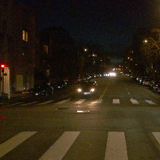
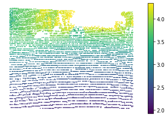
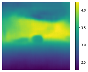
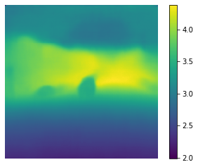
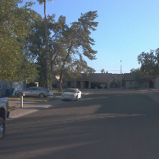
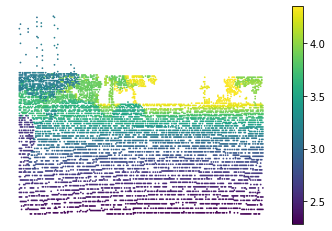
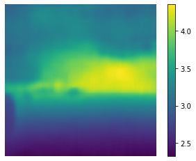
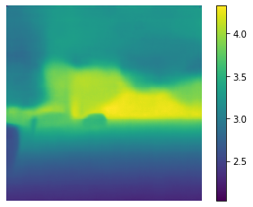
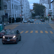
() Input frame

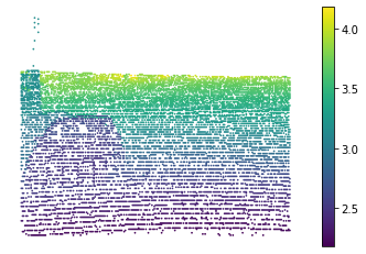
() Sparse depth target

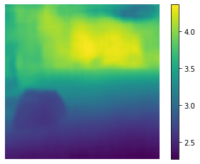
() DPT (ViT-L)

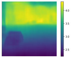
() DPT (ViT-e)

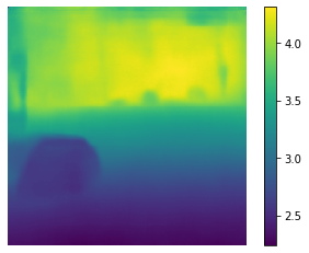
() DPT (ViT-22B)

Figure 13: Monocular depth estimation: (c, d, e) show estimated depth by a DPT head applied on ViT features, (a) shows the input frame and (b) shows the sparse ground-truth depth maps. Notice how (eg. in the third row) the model manages to go well beyond the available depth targets and makes what appear to be reasonable predictions for far-away cars, even though they are well out of LiDAR range. Ground-truth depth and depth predictions are visualized in $\log(1+\text{depth})$ space.

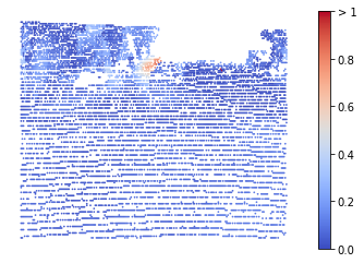
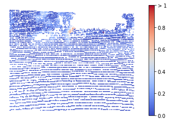
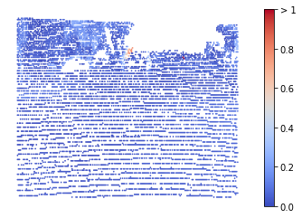
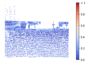
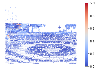
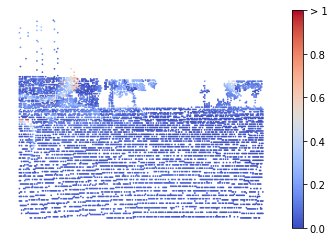
() Input frame

() Sparse depth target

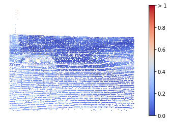
() DPT (ViT-L)

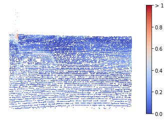
() DPT (ViT-e)

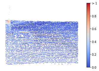
() DPT (ViT-22B)

Figure 14: Monocular depth estimation errors: (c, d, e) show absolute depth estimation errors by a DPT head applied on ViT features (for points where the ground truth is available), (a) shows the input frame and (b) shows the sparse ground truth depth maps. Notice how the outline of the car is clearly visible (light blue) from the sparse error maps in the third row when using ViT-L or ViT-e, while using ViT-22B leads to fewer errors in this region (darker blue). Ground-truth depth and absolute prediction errors are visualized in $\log(1+\text{depth})$ space.

Linear decoder.

The linear decoder processes $16\times 16\times 6144~{}$ ViT-22B feature maps using two transpose convolution layers of stride 2 and kernel size 5, followed by a $1\times 1$ convolution that outputs a low resolution depth map. This is resized to $224\times 224$ using bilinear interpolation and clipped at $0$ to be valid predictions for $log\left(1+\mathrm{depth}\right)$ The intermediate feature maps have $1536$ and $768$ dimensions each. Linear activations are used in between layers so that the whole decoder is end-to-end linear. This performed marginally better than a single $11\times 11$ stride $4$ transpose convolution layer, although the single layer decoder should be equally powerful in theory. We suspect that this has to do with how hyper-parameters have been empirically optimized for smaller kernel sizes.

For the ViT-e and ViT-L baselines, the linear decoder is exactly the same except for a much smaller input feature dimension ($1792$ for ViT-e and $1024$ for ViT-L). Thus the linear decoder on top of ViT-22B has more capacity than the same on top of ViT-e or ViT-l. We controlled for this in two ways: (a) using a $1\times 1$ convolution on the ViT-22B features, we down-project them to $1792$ dimensions to match the feature map size of ViT-e, or (b) using a large hidden dimension ($4096$ in ViT-e’s decoder and $6144$ in ViT-L’s decoder) after the first convolution transpose layer, we approximately matched the number of parameters across the three models. In control (a), performance stayed roughly the same at $0.165$ relative absolute error (AbsRel) for ViT-22B. In control (b) performance for baselines did not change substantially in terms of relative absolute error, $0.208$ for ViT-e and $0.222$ for ViT-L. We therefore report results without these controls in Table 5.

E.2.3 Training Details

We train the decoder for 300k steps with a batch size of 64 using Adam (Kingma and Ba, 2015) and clip the gradients to a global norm value of 0.05 to stabilize training. We linearly increase the learning rate for 2500 steps to 0.0002 (starting from 0) and then decay the learning rate with a cosine schedule (Loshchilov and Hutter, 2017) back to 0.

E.2.4 Metrics

We quantify performance using the following standard depth estimation metrics from the literature (Hermann et al., 2020; Eigen et al., 2014), and also report the MSE loss on the validation set: AbsRel measures the mean absolute error between the ground truth and predicted depth relative to the ground truth, while the inlier fraction metrics ($\delta$) measure the fraction of valid pixels within a certain percentage from ground truth. All metrics were measured after undoing the log transformation.

E.2.5 Qualitative Results

We report qualitative depth predictions by DPT from different ViT backbones in Figure 13, and absolute prediction errors in Figure 14.

Appendix F Video Classification

We sample 128 and 32 frames with a stride of 2 frames from Kinetics 400 videos (Kay et al., 2017) and Moments in Time (Monfort et al., 2019) videos, respectively. For both ViT-22B and ViT-e we rely in the frozen, pre-trained models and use the pre-logit feature representation to extract a single embedding per frame, resulting in a token sequences of length 128 and 32, respectively, which are then processed by a shallow transformer model equipped with a class-token classifier.

This is in contrast to CoCa (Yu et al., 2022a), which uses one token per image patch for their video classification experiments and a resolution of 576px (compared 224px in our experiments), resulting in much longer token sequences. We explored using one token per image patch (i.e. unpooled features) in preliminary experiments, but found that this leads to inferior performance. One potential reason for this could be that CoCa applies a contrastive loss to a pooled feature representation, and additionally feeds the unpooled token sequences to a generative decoder, which might lead to a different structure in the unpooled representation than the supervised classification loss used to pretrain ViT-22B and ViT-e.

To facilitate experimentation, we pre-compute frozen features for the two ViT variants we consider, using the same augmentations as (Arnab et al., 2021). To improve the robustness of our model and prevent overfitting we feed the entire training set ten times, with different data augmentations for every pass. We train for 30 epochs on these precomputed features with a batch size of 256 using SGD with momentum and with a cosine schedule including a linear warmup of 2.5 epochs. We sweep the following hyperparameters and corresponding value ranges to train our video model: $\{1,2\}$ transformer layers of width $\{1024,2048,4096\}$, using a learning rate in $\{10^{-1},10^{-2}\}$ and a weight decay in $\{10^{-3},10^{-2}\}$.

Appendix G Fairness

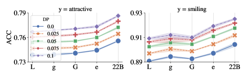
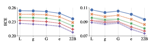
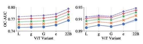
Figure 16: Performance, in terms of either accuracy (top), ECE (middle), or OC-AUC (bottom), is plotted for each ViT variant after debiasing the model to meet the prescribed level of bias shown in the legends. Refer to Section 4.5.1 for details.

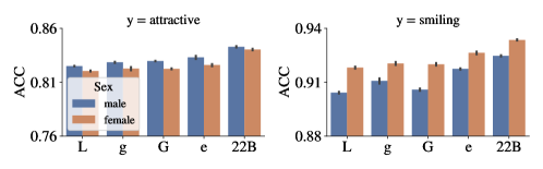
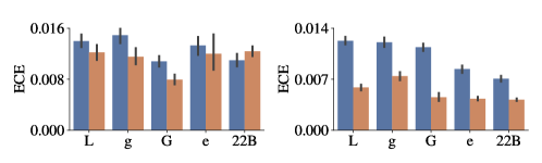
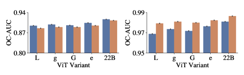
Figure 17: Performance is plotted for each subgroup in CelebA prior to bias mitigation. ViT-22B offers better performance overall across all three metrics, not just overall, but also within each subgroup separately. Refer to Section 4.5.1 for details.

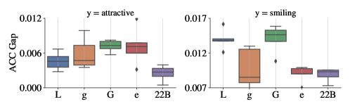
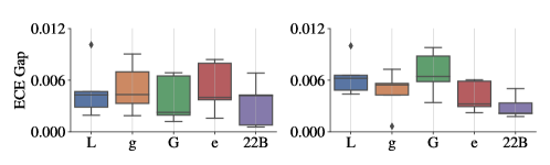
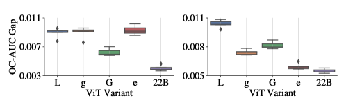
Figure 18: The $y$-axis is the absolute difference in performance across the two subgroups: females and males. ViT-22B provides a more equitable performance, compared to earlier/smaller ViT architectures in all three metrics.

We report the full experimental results described in Section 4.5.1 for all three evaluation (1) classification accuracy (denoted ACC), (2) expected calibration error (ECE) (Naeini et al., 2015; Guo et al., 2017), and (3) Oracle Collaborative AUC (OC-AUC) (Kivlichan et al., 2021). ECE is used to measure calibration, while OC-AUC computes the four variables: binned true/false positives/negatives, as a function of a linearly spaced set of thresholds and score bins. The full results are presented in Figure 16, Figure 17, and Figure 18.

Appendix H Calibration

We precisely follow the setup of Minderer et al. (2021): Since temperature scaling (Guo et al., 2017) requires some held-out data, we use 20% of the ImageNet validation set to learn the temperature parameter while we report the accuracy and expected calibration error on the remaining 80%.

Moreover, since the expected calibration error is defined with respect to a probability distribution normalised over the classes, we use a softmax loss function during fine tuning. The sigmoid loss function is defined independently across the classes and does not yield the required normalisation. We use 20k steps together with a learning rate of 0.03.

We reuse the plotting tools provided at https://github.com/google-research/robustness_metrics/tree/master/robustness_metrics/projects/revisiting_calibration.

Appendix I Plex

I.1 Details about the evaluation

We start by providing some details about the datasets and the different evaluation protocols based on Djolonga et al. (2020).

ImageNet-C (Hendrycks and Dietterich, 2019).

This variant of the ImageNet dataset contains algorithmically generated corruptions (e.g., blur and noise) applied to the ImageNet test-set. The results that we report in the paper are averaged over the 16 corruptions and over their 5 different intensity levels.

OOD detection (Hendrycks et al., 2019; Fort et al., 2021).

In this task, we try to classify whether a given test point belongs to the in-distribution dataset (in our case, ImageNet) or an out-of-distribution dataset (following Hendrycks et al. (2019); Tran et al. (2022), we take Places365 which consists of about 1.8 million images from 365 scene categories, where there are at most 5000 images per category (Zhou et al., 2017a)).

To perform the detection, we use the maximum softmax probability (MSP) (Hendrycks et al., 2019; Tran et al., 2022). We evaluate the performance of the resulting binary classification task thanks to the AUROC and AUPRC.

Selective prediction.

In this task, a model may defer its predictions to human experts when it is not confident enough. In particular, this task jointly assesses a model’s predictive performance and quality of uncertainty estimates (El-Yaniv and Wiener, 2010). Following Tran et al. (2022), we measure the performance with the oracle collaborative AUC (Kivlichan et al., 2021), with a review fraction of 0.5% of all predictions.

Label uncertainty.

For this evaluation, we aim at demonstrating the ability of the model to capture the inherent ambiguity of image labels assigned by humans. Following Tran et al. (2022), we focus on the ImageNet ReaL-H dataset that exploits the human ratings from Beyer et al. (2020) to construct a label distribution representing rater uncertainty for each image. The performance is measured by the negative log likelihood computed with respect to the soft labels (i.e., vectors in the simplex as opposed to the usual one-hot vectors).

I.2 Details about the Plex architecture

Plex (Tran et al., 2022) calls for BatchEnsemble layers (Wen et al., 2019) to be added in the model architecture during both pre-training and fine-tuning. Due to the high cost of training ViT-22B, we add the BatchEnsemble layers during the fine-tuning stage only. We replace all Dense layers in the ViT-22B, except for the Dense layer in the MLP layer for the pooling head with BatchEnsemble layers. Tran et al. (2022) further suggest to replace the final Dense layer of the network with a heteroscedastic output head (Collier et al., 2021). We thus follow this approach and evaluate both a heteroscedastic and BatchEnsemble final layer.

I.3 Details about the hyperparameters

All models were fine-tuned on ImageNet with a batch size 512. We swept over fine-tuning for 20k or 40k steps and learning rates of 0.01 and 0.03, with Plex models performing better at 40k fine-tuning steps—as already observed by Tran et al. (2022)—and learning rate of 0.03. Two BatchEnsemble members were used, with a random sign initialization in the BatchEnsemble layer of -0.5.

For the experiments with a heteroscedastic output layer, 1k MC samples were used and the low-rank component of the covariance matrix employed 15 factors. Furthermore, we report results for a temperature parameter of 5 (after a hyperparameter search over the [0.5, 10] range).

Unlike most of the models in the rest of the paper, the models of this section are fine tuned with a softmax loss function. We do so to be consistent with the design choices of Tran et al. (2022) and because a distribution normalised across the classes is required by several of the metrics employed (e.g., ECE).

I.4 Results of Plex-22B and challenges

In Table 15, we report the results of ViT-L/32, Plex-L/32, ViT-22B and the extensions of Plex to the 22B scale, Plex-22B, with the BatchEnsemble (BE) and heteroscedastic (HET) heads. All the models are fine tuned with a resolution of 384.

The main observation is that the increased scale of ViT-22B comes with substantial improvements across all metrics, except for the label uncertainty over ImageNet-ReaL-H.

More surprisingly, we can see that across all metrics (except for the label uncertainty over ImageNet-ReaL-H), the Plex-22B variants perform worse than the vanilla ViT-22B model. This observation does not extend the findings from Tran et al. (2022) where Plex consistently leads to improvement at the S, B and L scales.

We believe that this surprising observation may be related to specific challenges faced at the 22B scale:

• Pre-training vs. fine-tuning: While Tran et al. (2022) introduce BatchEnsemble layers already at pre-training time, the high training cost of ViT-22B forces us to only operate at fine-tuning time. In this regime, it may not be possible to properly learn the BatchEnsemble and heteroscedastic layers. Moreover, while fine-tuning with standard ViT backbones enjoys a well-performing and robust recipe, namely initializing the final Dense layer kernel to all zeros, we do not have an equivalent approach when adding the Plex components.

• Hyperparameter tuning: Even though we already covered a reasonable combination of hyperparameters (fine-tuning duration, learning rate and temperature), it is possible that a finer-grained search is required to close the performance gap.

• Numerical stability: As discussed in Section 2, it was required to use particular techniques to stabilize the training of ViT-22B. We hypothesise that similar techniques may have to be developed specifically for the Plex components (BatchEnsemble and heteroscedastic layers) to keep their efficiency at this scale.

Table 15: Evaluation on some representative metrics from the Plex reliability benchmark (Tran et al., 2022).

		IN-C (mean over shifts)					IN vs. Places365			IN-ReaL-H
Metrics		ACC $\uparrow$	NLL $\downarrow$	ECE $\downarrow$	OC-AUC $\uparrow$		AUROC $\uparrow$	AUPRC $\uparrow$		NLL $\downarrow$
ViT-L/32 (Tran et al., 2022)		70.1	1.28	0.05	0.91		0.83	0.96		1.09
Plex-L/32 (Tran et al., 2022)		71.3	1.21	0.02	0.91		0.83	0.97		1.03
ViT-22B		83.7	0.63	0.01	0.97		0.88	0.98		1.21
Plex-22B [BE]		81.0	0.98	0.18	0.95		0.86	0.98		0.94
Plex-22B [HET]		80.9	0.97	0.17	0.94		0.86	0.97		0.93

Appendix J Error Consistency & Human Alignment

In Section 4.5.2, we described results for testing ViT-22B fine-tuned on ImageNet on the model-vs-human benchmark. In Figure 19(a), Figure 19(b), Figure 19(c), Figure 19(d), we provide additional benchmarking results.

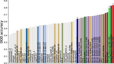
(a) OOD accuracy (higher = better).

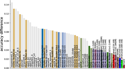
(b) Accuracy difference (lower = better).

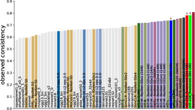
(c) Observed consistency (higher = better).

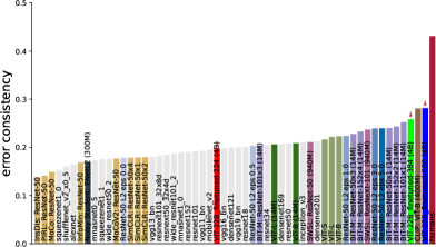
(d) Error consistency (higher = better).

Figure 19: Model-vs-human (Geirhos et al., 2021) benchmarking results for ViT-22B models fine-tuned on ImageNet with different resolutions (indicated by a red arrow). Results are aggregated over 17 challenging out-of-distribution (OOD) datasets from (Geirhos et al., 2021). OOD accuracy in Figure 19(a) is simply the accuracy across those datasets; accuracy difference in Figure 19(b) denotes the difference to human accuracies (either too low or too high is penalized); observed consistency in Figure 19(c) shows unnormalized image-level consistency (see Geirhos et al., 2021, for details) while Figure 19(d) shows error consistency (normalizes observed consistency by the consistency expected purely by change). Error consistency is only above zero if models and humans systematically agree in terms of which images are easy/difficult (correct/incorrect classification). Overall, while the three ViT-22B variants trained with different resolutions vary in their performance, a ViT-22B variant leads the leaderboard in all four metrics. Comparison models include standard CNNs (grey), adversarially trained models (blue), self-supervised models (orange) as well as other models evaluated by Geirhos et al. (2021).

Appendix K Perceptual similarity

Kumar et al. (2022) show a trade-off between the accuracy of latest ImageNet classifiers and their inherent ability to capture perceptual similarity. Here, we explore if large-scale classification on a more diverse training dataset than ImageNet can break the observed trade-off. To compare the perceptual similarity of ViT-22B with prior ImageNet-trained models, we make minor changes to adapt ViT-22B on low resolution $64\times 64$ ImageNet. ViT-22B fine-tuned on ImageNet $64\times 64$ achieves 84.2 accuracy on ImageNet $64\times 64$ which is $16\%$ better than the best models trained directly on ImageNet. As done in (Zhang et al., 2018), we assess the ability of ViT-22B to capture perceptual similarity using 48 intermediate representations. The perceptual score of ViT-22B (64.9) is much lower than all other models, indicating that models trained on large-scale classification also lie on the observed accuracy-perceptual similarity Pareto Frontier.

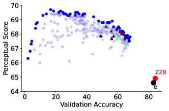
Figure 20: ViT-22B lies on the bottom-right of the accuracy-perceptual similarity tradeoff. It achieves the best validation accuracy on $64\times 64$ ImageNet with the worst perceptual scores.

To make a fair comparison with the models in (Kumar et al., 2022), we make minor changes to adapt ViT-22B on low resolution $64\times 64$ ImageNet. Directly finetuneing ViT-22B on $64\times 64$ images with the default patch-size of 14 leads to two undesirable consequences a) A low sequence length of 16 and b) Cropping of 8 pixels on the right borders. So, as proposed in (Beyer et al., 2022a), we resize the trained embedding layer from the default patch-size of 14 to a patch-size of 8 that leads to a longer sequence length of 64. Then, we adapt standard finetuneing protocols.

We make three more observations: 1) Untrained ViT-22B gets a even lower Perceptual Score of 62.3, thus some amount of training is desirable 2) ViT-e lies in the same ballpark as ViT-22B with slightly lower accuracy and Perceptual Scores 3) ViT-22B with the newly proposed Mean Pool distance function (Kumar et al., 2022) can improve its Perceptual Score up to 66.2.

Appendix L Feature attribution analysis

To get a better understanding on how ViT-22B arrives at its predictions we make use of gradient-based feature attribution methods (a.k.a. saliency maps). Figure 21 shows the result of applying Integrated Gradients (Sundararajan et al., 2017, IG) to three example datapoints before and after ViT-22B cooldown. We find that using a gray (0.5) baseline and 1024 steps yields qualitatively the best results. The images show a subtle difference in how the two model checkpoints process the example inputs, where more yellow indicates a higher sensitivity. We can also clearly see the patches in which ViT-22B processes input images. This means that the model is less sensitive around the edges of each patch, and suggests a path for future work to improve the model to better deal with patch edges.

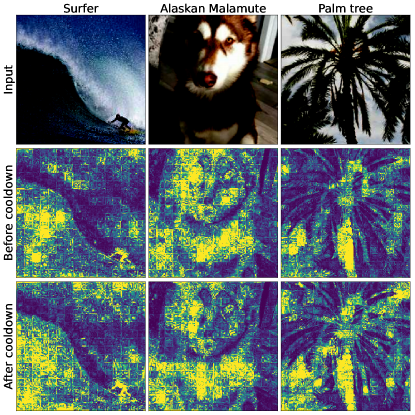
Figure 21: Saliency before and after model cooldown.

References

- Abnar et al. (2021) Samira Abnar, Mostafa Dehghani, Behnam Neyshabur, and Hanie Sedghi. Exploring the limits of large scale pre-training. arXiv preprint arXiv:2110.02095, 2021.
- Adler et al. (2020) Thomas Adler, Johannes Brandstetter, Michael Widrich, Andreas Mayr, David P. Kreil, Michael Kopp, Günter Klambauer, and Sepp Hochreiter. Cross-domain few-shot learning by representation fusion. arXiv preprint arXiv:2010.06498, 2020.
- Aka et al. (2021) Osman Aka, Ken Burke, Alex Bauerle, Christina Greer, and Margaret Mitchell. Measuring model biases in the absence of ground truth. In Proceedings of the 2021 AAAI/ACM Conference on AI, Ethics, and Society, pages 327–335, 2021.
- Alabdulmohsin and Lucic (2021) Ibrahim Alabdulmohsin and Mario Lucic. A near optimal algorithm for debiasing trained machine learning models. In NeurIPS, 2021.
- Andreassen et al. (2021) Anders Andreassen, Yasaman Bahri, Behnam Neyshabur, and Rebecca Roelofs. The evolution of out-of-distribution robustness throughout fine-tuning. arXiv preprint arXiv:2106.15831, 2021.
- Arnab et al. (2021) Anurag Arnab, Mostafa Dehghani, Georg Heigold, Chen Sun, Mario Lučić, and Cordelia Schmid. ViViT: A video vision transformer. In CVPR, 2021.
- Ba et al. (2016) Jimmy Lei Ba, Jamie Ryan Kiros, and Geoffrey E Hinton. Layer normalization. arXiv preprint arXiv:1607.06450, 2016.
- Barbu et al. (2019) Andrei Barbu, David Mayo, Julian Alverio, William Luo, Christopher Wang, Dan Gutfreund, Josh Tenenbaum, and Boris Katz. ObjectNet: A large-scale bias-controlled dataset for pushing the limits of object recognition models. In NeurIPS, pages 9448–9458, 2019.
- Beattie et al. (2016) Charles Beattie, Joel Z Leibo, Denis Teplyashin, Tom Ward, Marcus Wainwright, Heinrich Küttler, Andrew Lefrancq, Simon Green, Víctor Valdés, Amir Sadik, et al. Deepmind lab. arXiv preprint arXiv:1612.03801, 2016.
- Beyer et al. (2020) Lucas Beyer, Olivier J Hénaff, Alexander Kolesnikov, Xiaohua Zhai, and Aäron van den Oord. Are we done with imagenet? arXiv preprint arXiv:2006.07159, 2020.
- Beyer et al. (2022a) Lucas Beyer, Pavel Izmailov, Alexander Kolesnikov, Mathilde Caron, Simon Kornblith, Xiaohua Zhai, Matthias Minderer, Michael Tschannen, Ibrahim Alabdulmohsin, and Filip Pavetic. Flexivit: One model for all patch sizes. arXiv preprint arXiv:2212.08013, 2022a.
- Beyer et al. (2022b) Lucas Beyer, Xiaohua Zhai, Amélie Royer, Larisa Markeeva, Rohan Anil, and Alexander Kolesnikov. Knowledge distillation: A good teacher is patient and consistent. In CVPR, pages 10925–10934, 2022b.
- Bradbury et al. (2018) James Bradbury, Roy Frostig, Peter Hawkins, Matthew James Johnson, Chris Leary, Dougal Maclaurin, George Necula, Adam Paszke, Jake VanderPlas, Skye Wanderman-Milne, and Qiao Zhang. JAX: composable transformations of Python+NumPy programs, 2018. URL http://github.com/google/jax.
- Buolamwini and Gebru (2018) Joy Buolamwini and Timnit Gebru. Gender shades: Intersectional accuracy disparities in commercial gender classification. In FAccT, 2018.
- Byrd et al. (1995) Richard H Byrd, Peihuang Lu, Jorge Nocedal, and Ciyou Zhu. A limited memory algorithm for bound constrained optimization. SIAM Journal on scientific computing, 16(5):1190–1208, 1995.
- Caliskan et al. (2017) Aylin Caliskan, Joanna J Bryson, and Arvind Narayanan. Semantics derived automatically from language corpora contain human-like biases. Science, 356(6334), 2017.
- Chen et al. (2022) Xi Chen, Xiao Wang, Soravit Changpinyo, A. J. Piergiovanni, Piotr Padlewski, Daniel Salz, Sebastian Goodman, Adam Grycner, Basil Mustafa, Lucas Beyer, Alexander Kolesnikov, Joan Puigcerver, Nan Ding, Keran Rong, Hassan Akbari, Gaurav Mishra, Linting Xue, Ashish Thapliyal, James Bradbury, Weicheng Kuo, Mojtaba Seyedhosseini, Chao Jia, Burcu Karagol Ayan, Carlos Riquelme, Andreas Steiner, Anelia Angelova, Xiaohua Zhai, Neil Houlsby, and Radu Soricut. PaLI: A jointly-scaled multilingual language-image model. arXiv preprint arXiv:2209.06794, 2022.
- Cheng et al. (2017) Gong Cheng, Junwei Han, and Xiaoqiang Lu. Remote sensing image scene classification: Benchmark and state of the art. Proceedings of the IEEE, 105(10):1865–1883, 2017.
- Chowdhery et al. (2022) Aakanksha Chowdhery, Sharan Narang, Jacob Devlin, Maarten Bosma, Gaurav Mishra, Adam Roberts, Paul Barham, Hyung Won Chung, Charles Sutton, Sebastian Gehrmann, et al. PaLM: Scaling language modeling with pathways. arXiv preprint arXiv:2204.02311, 2022.
- Chung et al. (2022) Hyung Won Chung, Le Hou, Shayne Longpre, Barret Zoph, Yi Tay, William Fedus, Eric Li, Xuezhi Wang, Mostafa Dehghani, Siddhartha Brahma, et al. Scaling instruction-finetuned language models. arXiv preprint arXiv:2210.11416, 2022.
- Cimpoi et al. (2014) Mircea Cimpoi, Subhransu Maji, Iasonas Kokkinos, Sammy Mohamed, and Andrea Vedaldi. Describing textures in the wild. In CVPR, pages 3606–3613, 2014.
- Collier et al. (2021) Mark Collier, Basil Mustafa, Efi Kokiopoulou, Rodolphe Jenatton, and Jesse Berent. Correlated input-dependent label noise in large-scale image classification. In CVPR, pages 1551–1560, 2021.
- Cordonnier et al. (2019) Jean-Baptiste Cordonnier, Andreas Loukas, and Martin Jaggi. On the relationship between self-attention and convolutional layers. arXiv preprint arXiv:1911.03584, 2019.
- Cui et al. (2018) Yin Cui, Yang Song, Chen Sun, Andrew Howard, and Serge Belongie. Large scale fine-grained categorization and domain-specific transfer learning. In CVPR, pages 4109–4118, 2018.
- Dehghani et al. (2021a) Mostafa Dehghani, Anurag Arnab, Lucas Beyer, Ashish Vaswani, and Yi Tay. The efficiency misnomer. arXiv preprint arXiv:2110.12894, 2021a.
- Dehghani et al. (2021b) Mostafa Dehghani, Yi Tay, Alexey A Gritsenko, Zhe Zhao, Neil Houlsby, Fernando Diaz, Donald Metzler, and Oriol Vinyals. The benchmark lottery. arXiv preprint arXiv:2107.07002, 2021b.
- Dehghani et al. (2022) Mostafa Dehghani, Alexey Gritsenko, Anurag Arnab, Matthias Minderer, and Yi Tay. Scenic: A jax library for computer vision research and beyond. In CVPR, 2022.
- Deng et al. (2009) Jia Deng, Wei Dong, Richard Socher, Li-Jia Li, Kai Li, and Li Fei-Fei. ImageNet: A large-scale hierarchical image database. In CVPR, pages 248–255, 2009.
- Deuschel et al. (2020) Jessica Deuschel, Bettina Finzel, and Ines Rieger. Uncovering the bias in facial expressions. arXiv preprint arXiv:2011.11311, 2020.
- Djolonga et al. (2020) Josip Djolonga, Frances Hubis, Matthias Minderer, Zachary Nado, Jeremy Nixon, Rob Romijnders, Dustin Tran, and Mario Lucic. Robustness Metrics, 2020. URL https://github.com/google-research/robustness_metrics.
- Djolonga et al. (2021) Josip Djolonga, Jessica Yung, Michael Tschannen, Rob Romijnders, Lucas Beyer, Alexander Kolesnikov, Joan Puigcerver, Matthias Minderer, Alexander D’Amour, Dan Moldovan, Sylvain Gelly, Neil Houlsby, Xiaohua Zhai, and Mario Lucic. On robustness and transferability of convolutional neural networks. In CVPR, pages 16458–16468, 2021.
- Dosovitskiy et al. (2021) Alexey Dosovitskiy, Lucas Beyer, Alexander Kolesnikov, Dirk Weissenborn, Xiaohua Zhai, Thomas Unterthiner, Mostafa Dehghani, Matthias Minderer, Georg Heigold, Sylvain Gelly, Jakob Uszkoreit, and Neil Houlsby. An image is worth 16x16 words: Transformers for image recognition at scale. In ICLR, 2021.
- Dwork et al. (2012) Cynthia Dwork, Moritz Hardt, Toniann Pitassi, Omer Reingold, and Richard Zemel. Fairness through awareness. In Innovations in Theoretical Computer Science, 2012.
- Eigen et al. (2014) David Eigen, Christian Puhrsch, and Rob Fergus. Depth map prediction from a single image using a multi-scale deep network. In NeurIPS, 2014.
- El-Yaniv and Wiener (2010) Ran El-Yaniv and Yair Wiener. On the foundations of noise-free selective classification. Journal of Machine Learning Research, 11(5), 2010.
- Evci et al. (2022) Utku Evci, Vincent Dumoulin, Hugo Larochelle, and Michael C Mozer. Head2Toe: Utilizing intermediate representations for better transfer learning. In ICML, 2022.
- Everingham et al. (2010) Mark Everingham, Luc Van Gool, Christopher KI Williams, John Winn, and Andrew Zisserman. The pascal visual object classes (VOC) challenge. IJCV, 2010.
- Fedus et al. (2021) William Fedus, Barret Zoph, and Noam Shazeer. Switch transformers: Scaling to trillion parameter models with simple and efficient sparsity, 2021.
- Fort et al. (2021) Stanislav Fort, Jie Ren, and Balaji Lakshminarayanan. Exploring the limits of out-of-distribution detection. In NeurIPS, pages 7068–7081, 2021.
- Geiger et al. (2013) Andreas Geiger, Philip Lenz, Christoph Stiller, and Raquel Urtasun. Vision meets robotics: The kitti dataset. The International Journal of Robotics Research, 32(11):1231–1237, 2013.
- Geirhos et al. (2019) Robert Geirhos, Patricia Rubisch, Claudio Michaelis, Matthias Bethge, Felix A Wichmann, and Wieland Brendel. ImageNet-trained CNNs are biased towards texture; increasing shape bias improves accuracy and robustness. In ICLR, 2019.
- Geirhos et al. (2021) Robert Geirhos, Kantharaju Narayanappa, Benjamin Mitzkus, Tizian Thieringer, Matthias Bethge, Felix A Wichmann, and Wieland Brendel. Partial success in closing the gap between human and machine vision. In NeurIPS, pages 23885–23899, 2021.
- Gilmer et al. (2023) Justin Gilmer, Andrea Schioppa, and Jeremy Cohen. Intriguing Properties of Transformer Training Instabilities, 2023. To appear.
- Guo et al. (2017) Chuan Guo, Geoff Pleiss, Yu Sun, and Kilian Q Weinberger. On calibration of modern neural networks. In ICML, 2017.
- Heek et al. (2020) Jonathan Heek, Anselm Levskaya, Avital Oliver, Marvin Ritter, Bertrand Rondepierre, Andreas Steiner, and Marc van Zee. Flax: A neural network library and ecosystem for JAX, 2020. URL http://github.com/google/flax.
- Helber et al. (2019) Patrick Helber, Benjamin Bischke, Andreas Dengel, and Damian Borth. Eurosat: A novel dataset and deep learning benchmark for land use and land cover classification. IEEE Journal of Selected Topics in Applied Earth Observations and Remote Sensing, 12(7):2217–2226, 2019.
- Hendricks et al. (2018) Lisa Anne Hendricks, Kaylee Burns, Kate Saenko, Trevor Darrell, and Anna Rohrbach. Women also snowboard: Overcoming bias in captioning models. In ECCV, 2018.
- Hendrycks and Dietterich (2019) Dan Hendrycks and Thomas Dietterich. Benchmarking neural network robustness to common corruptions and perturbations. arXiv preprint arXiv:1903.12261, 2019.
- Hendrycks et al. (2019) Dan Hendrycks, Steven Basart, Mantas Mazeika, Mohammadreza Mostajabi, Jacob Steinhardt, and Dawn Song. Scaling out-of-distribution detection for real-world settings. arXiv preprint arXiv:1911.11132, 2019.
- Hendrycks et al. (2020) Dan Hendrycks, Steven Basart, Norman Mu, Saurav Kadavath, Frank Wang, Evan Dorundo, Rahul Desai, Tyler Zhu, Samyak Parajuli, Mike Guo, Dawn Song, Jacob Steinhardt, and Justin Gilmer. The many faces of robustness: A critical analysis of out-of-distribution generalization. arXiv preprint arXiv:2006.16241, 2020.
- Hendrycks et al. (2021) Dan Hendrycks, Kevin Zhao, Steven Basart, Jacob Steinhardt, and Dawn Song. Natural adversarial examples. In CVPR, pages 15262–15271, 2021.
- Hermann et al. (2020) Max Hermann, Boitumelo Ruf, Martin Weinmann, and Stefan Hinz. Self-supervised learning for monocular depth estimation from aerial imagery. arXiv preprint arXiv:2008.07246, 2020.
- Hinton et al. (2015) Geoffrey Hinton, Oriol Vinyals, Jeff Dean, et al. Distilling the knowledge in a neural network. arXiv preprint arXiv:1503.02531, 2(7), 2015.
- Jia et al. (2021) Chao Jia, Yinfei Yang, Ye Xia, Yi-Ting Chen, Zarana Parekh, Hieu Pham, Quoc Le, Yun-Hsuan Sung, Zhen Li, and Tom Duerig. Scaling up visual and vision-language representation learning with noisy text supervision. In ICML, pages 4904–4916, 2021.
- Johnson et al. (2017) Justin Johnson, Bharath Hariharan, Laurens Van Der Maaten, Li Fei-Fei, C Lawrence Zitnick, and Ross Girshick. CLEVR: A diagnostic dataset for compositional language and elementary visual reasoning. In CVPR, pages 2901–2910, 2017.
- Jouppi et al. (2020) Norman P Jouppi, Doe Hyun Yoon, George Kurian, Sheng Li, Nishant Patil, James Laudon, Cliff Young, and David Patterson. A domain-specific supercomputer for training deep neural networks. Communications of the ACM, 63(7):67–78, 2020.
- Kaggle and EyePacs (2015) Kaggle and EyePacs. Kaggle diabetic retinopathy detection, 2015. URL https://www.kaggle.com/c/diabetic-retinopathy-detection/data.
- Kather et al. (2016) Jakob Nikolas Kather, Cleo-Aron Weis, Francesco Bianconi, Susanne M Melchers, Lothar R Schad, Timo Gaiser, Alexander Marx, and Frank Gerrit Zöllner. Multi-class texture analysis in colorectal cancer histology. Scientific reports, 6:27988, 2016.
- Kay et al. (2017) Will Kay, Joao Carreira, Karen Simonyan, Brian Zhang, Chloe Hillier, Sudheendra Vijayanarasimhan, Fabio Viola, Tim Green, Trevor Back, Paul Natsev, et al. The kinetics human action video dataset. arXiv preprint arXiv:1705.06950, 2017.
- Khalifa et al. (2022) Amr Khalifa, Michael C. Mozer, Hanie Sedghi, Behnam Neyshabur, and Ibrahim Alabdulmohsin. Layer-stack temperature scaling. arXiv preprint arXiv:2211.10193, 2022.
- Kingma and Ba (2015) Diederik P Kingma and Jimmy Ba. Adam: A method for stochastic optimization. In ICLR, 2015.
- Kivlichan et al. (2021) Ian D Kivlichan, Zi Lin, Jeremiah Liu, and Lucy Vasserman. Measuring and improving model-moderator collaboration using uncertainty estimation. arXiv preprint arXiv:2107.04212, 2021.
- Kolesnikov et al. (2020) Alexander Kolesnikov, Lucas Beyer, Xiaohua Zhai, Joan Puigcerver, Jessica Yung, Sylvain Gelly, and Neil Houlsby. Big Transfer (BiT): General visual representation learning. In ECCV, pages 491–507, 2020.
- Krause et al. (2013) Jonathan Krause, Michael Stark, Jia Deng, and Li Fei-Fei. 3d object representations for fine-grained categorization. In 4th International IEEE Workshop on 3D Representation and Recognition, 2013.
- Krizhevsky et al. (2009) Alex Krizhevsky, Geoffrey Hinton, et al. Learning multiple layers of features from tiny images, 2009. Technical Report, University of Toronto.
- Kudo and Richardson (2018) Taku Kudo and John Richardson. SentencePiece: A simple and language independent subword tokenizer and detokenizer for neural text processing. In EMNLP, pages 66–71, November 2018.
- Kumar et al. (2022) Manoj Kumar, Neil Houlsby, Nal Kalchbrenner, and Ekin Dogus Cubuk. Do better imagenet classifiers assess perceptual similarity better? Transactions on Machine Learning Research, 2022.
- LeCun et al. (2004) Yann LeCun, Fu Jie Huang, and Leon Bottou. Learning methods for generic object recognition with invariance to pose and lighting. In CVPR, volume 2, 2004.
- Li et al. (2022) Fei-Fei Li, Marco Andreeto, Marc’Aurelio Ranzato, and Pietro Perona. Caltech 101, 2022. CaltechDATA, doi: 10.22002/D1.20086.
- Liu et al. (2015) Ziwei Liu, Ping Luo, Xiaogang Wang, and Xiaoou Tang. Deep learning face attributes in the wild. In ICCV, 2015.
- Loshchilov and Hutter (2017) Ilya Loshchilov and Frank Hutter. SGDR: Stochastic gradient descent with warm restarts. In ICLR, 2017.
- Mahajan et al. (2018) Dhruv Mahajan, Ross Girshick, Vignesh Ramanathan, Kaiming He, Manohar Paluri, Yixuan Li, Ashwin Bharambe, and Laurens Van Der Maaten. Exploring the limits of weakly supervised pretraining. In ECCV, pages 181–196, 2018.
- Matthey et al. (2017) Loic Matthey, Irina Higgins, Demis Hassabis, and Alexander Lerchner. dSprites: Disentanglement testing sprites dataset, 2017. URL https://github.com/deepmind/dsprites-dataset/.
- Minderer et al. (2021) Matthias Minderer, Josip Djolonga, Rob Romijnders, Frances Hubis, Xiaohua Zhai, Neil Houlsby, Dustin Tran, and Mario Lucic. Revisiting the calibration of modern neural networks. NeurIPS, 34:15682–15694, 2021.
- Mitchell et al. (2019) Margaret Mitchell, Simone Wu, Andrew Zaldivar, Parker Barnes, Lucy Vasserman, Ben Hutchinson, Elena Spitzer, Inioluwa Deborah Raji, and Timnit Gebru. Model cards for model reporting. In FAccT, pages 220–229, 2019.
- Monfort et al. (2019) Mathew Monfort, Alex Andonian, Bolei Zhou, Kandan Ramakrishnan, Sarah Adel Bargal, Tom Yan, Lisa Brown, Quanfu Fan, Dan Gutfreund, Carl Vondrick, et al. Moments in time dataset: one million videos for event understanding. IEEE Transactions on Pattern Analysis and Machine Intelligence, 42(2), 2019.
- Mottaghi et al. (2014) Roozbeh Mottaghi, Xianjie Chen, Xiaobai Liu, Nam-Gyu Cho, Seong-Whan Lee, Sanja Fidler, Raquel Urtasun, and Alan Yuille. The role of context for object detection and semantic segmentation in the wild. In CVPR, 2014.
- Naeini et al. (2015) Mahdi Pakdaman Naeini, Gregory Cooper, and Milos Hauskrecht. Obtaining well calibrated probabilities using bayesian binning. In AAAI, 2015.
- Netzer et al. (2011) Yuval Netzer, Tao Wang, Adam Coates, Alessandro Bissacco, Bo Wu, and Andrew Y. Ng. Reading digits in natural images with unsupervised feature learning. In NIPS Workshop on Deep Learning and Unsupervised Feature Learning 2011, 2011.
- Nilsback and Zisserman (2008) Maria-Elena Nilsback and Andrew Zisserman. Automated flower classification over a large number of classes. In Indian Conference on Computer Vision, Graphics & Image Processing, pages 722–729, 2008.
- Pan and Yang (2010) Sinno Jialin Pan and Qiang Yang. A survey on transfer learning. IEEE Transactions on Knowledge and Data Engineering, 22(10):1345–1359, 2010.
- Parkhi et al. (2012) Omkar M Parkhi, Andrea Vedaldi, Andrew Zisserman, and CV Jawahar. Cats and dogs. In 2012 IEEE conference on computer vision and pattern recognition, pages 3498–3505. IEEE, 2012.
- Pham et al. (2021) Hieu Pham, Zihang Dai, Golnaz Ghiasi, Hanxiao Liu, Adams Wei Yu, Minh-Thang Luong, Mingxing Tan, and Quoc V Le. Combined scaling for zero-shot transfer learning. arXiv preprint arXiv:2111.10050, 2021.
- Pope et al. (2022) Reiner Pope, Sholto Douglas, Aakanksha Chowdhery, Jacob Devlin, James Bradbury, Anselm Levskaya, Jonathan Heek, Kefan Xiao, Shivani Agrawal, and Jeff Dean. Efficiently scaling transformer inference. arXiv preprint arXiv:2211.05102, 2022.
- Radford et al. (2021) Alec Radford, Jong Wook Kim, Chris Hallacy, Aditya Ramesh, Gabriel Goh, Sandhini Agarwal, Girish Sastry, Amanda Askell, Pamela Mishkin, Jack Clark, et al. Learning transferable visual models from natural language supervision. In ICML, pages 8748–8763, 2021.
- Raffel et al. (2019) Colin Raffel, Noam Shazeer, Adam Roberts, Katherine Lee, Sharan Narang, Michael Matena, Yanqi Zhou, Wei Li, and Peter J. Liu. Exploring the limits of transfer learning with a unified text-to-text transformer. arXiv preprint arXiv:1910.10683, 2019.
- Ranftl et al. (2021) René Ranftl, Alexey Bochkovskiy, and Vladlen Koltun. Vision transformers for dense prediction. In CVPR, pages 12179–12188, 2021.
- Recht et al. (2019) Benjamin Recht, Rebecca Roelofs, Ludwig Schmidt, and Vaishaal Shankar. Do ImageNet classifiers generalize to ImageNet? In ICML, 2019.
- Riquelme et al. (2021) Carlos Riquelme, Joan Puigcerver, Basil Mustafa, Maxim Neumann, Rodolphe Jenatton, André Susano Pinto, Daniel Keysers, and Neil Houlsby. Scaling vision with sparse mixture of experts. In NeurIPS, volume 34, pages 8583–8595, 2021.
- Saharia et al. (2022) Chitwan Saharia, William Chan, Saurabh Saxena, Lala Li, Jay Whang, Emily Denton, Seyed Kamyar Seyed Ghasemipour, Burcu Karagol Ayan, S Sara Mahdavi, Rapha Gontijo Lopes, et al. Photorealistic text-to-image diffusion models with deep language understanding. NeurIPS, 2022.
- Strudel et al. (2021) Robin Strudel, Ricardo Garcia, Ivan Laptev, and Cordelia Schmid. Segmenter: Transformer for semantic segmentation. In ICCV, 2021.
- Sun et al. (2017) Chen Sun, Abhinav Shrivastava, Saurabh Singh, and Abhinav Gupta. Revisiting unreasonable effectiveness of data in deep learning era. In CVPR, pages 843–852, 2017.
- Sun et al. (2020) Pei Sun, Henrik Kretzschmar, Xerxes Dotiwalla, Aurelien Chouard, Vijaysai Patnaik, Paul Tsui, James Guo, Yin Zhou, Yuning Chai, Benjamin Caine, et al. Scalability in perception for autonomous driving: Waymo open dataset. In CVPR, 2020.
- Sundararajan et al. (2017) Mukund Sundararajan, Ankur Taly, and Qiqi Yan. Axiomatic attribution for deep networks. In ICML, pages 3319–3328, 2017.
- Szegedy et al. (2015) Christian Szegedy, Wei Liu, Yangqing Jia, Pierre Sermanet, Scott Reed, Dragomir Anguelov, Dumitru Erhan, Vincent Vanhoucke, and Andrew Rabinovich. Going deeper with convolutions. In CVPR, 2015.
- Taori et al. (2020) Rohan Taori, Achal Dave, Vaishaal Shankar, Nicholas Carlini, Benjamin Recht, and Ludwig Schmidt. Measuring robustness to natural distribution shifts in image classification. In NeurIPS, 2020.
- Tay et al. (2022) Yi Tay, Mostafa Dehghani, Vinh Q Tran, Xavier Garcia, Dara Bahri, Tal Schuster, Huaixiu Steven Zheng, Neil Houlsby, and Donald Metzler. Unifying language learning paradigms. arXiv preprint arXiv:2205.05131, 2022.
- Teh and Taylor (2019) Eu Wern Teh and Graham W Taylor. Metric learning for patch classification in digital pathology. In International Conference on Medical Imaging with Deep Learning–Extended Abstract Track, 2019.
- Touvron et al. (2022) Hugo Touvron, Matthieu Cord, and Hervé Jégou. DeiT III: Revenge of the ViT. In ECCV, 2022.
- Tran et al. (2022) Dustin Tran, Jeremiah Liu, Michael W Dusenberry, Du Phan, Mark Collier, Jie Ren, Kehang Han, Zi Wang, Zelda Mariet, Huiyi Hu, et al. Plex: Towards reliability using pretrained large model extensions. arXiv preprint arXiv:2207.07411, 2022.
- Wah et al. (2011) C. Wah, S. Branson, P. Welinder, P. Perona, and S. Belongie. The Caltech-UCSD Birds-200-2011 dataset. Technical Report CNS-TR-2011-001, California Institute of Technology, 2011.
- Wang and Komatsuzaki (2021) Ben Wang and Aran Komatsuzaki. GPT-J-6B: A 6 Billion Parameter Autoregressive Language Model. https://github.com/kingoflolz/mesh-transformer-jax, May 2021.
- Wang et al. (2022a) Shibo Wang, Jinliang Wei, Amit Sabne, Andy Davis, Berkin Ilbeyi, Blake Hechtman, Dehao Chen, Karthik Srinivasa Murthy, Marcello Maggioni, Qiao Zhang, Sameer Kumar, Tongfei Guo, Yuanzhong Xu, and Zongwei Zhou. Overlap communication with dependent computation via decomposition in large deep learning models. In ACM International Conference on Architectural Support for Programming Languages and Operating Systems, pages 93––106, 2022a.
- Wang et al. (2022b) Yi Wang, Kunchang Li, Yizhuo Li, Yinan He, Bingkun Huang, Zhiyu Zhao, Hongjie Zhang, Jilan Xu, Yi Liu, Zun Wang, Sen Xing, Guo Chen, Junting Pan, Jiashuo Yu, Yali Wang, Limin Wang, and Yu Qiao. Internvideo: General video foundation models via generative and discriminative learning. arXiv preprint arXiv:2212.03191, 2022b.
- Wang et al. (2020) Zeyu Wang, Klint Qinami, Ioannis Christos Karakozis, Kyle Genova, Prem Nair, Kenji Hata, and Olga Russakovsky. Towards fairness in visual recognition: Effective strategies for bias mitigation. In CVPR, 2020.
- Wei et al. (2022) Jason Wei, Yi Tay, Rishi Bommasani, Colin Raffel, Barret Zoph, Sebastian Borgeaud, Dani Yogatama, Maarten Bosma, Denny Zhou, Donald Metzler, et al. Emergent abilities of large language models. arXiv preprint arXiv:2206.07682, 2022.
- Wen et al. (2019) Yeming Wen, Dustin Tran, and Jimmy Ba. Batchensemble: an alternative approach to efficient ensemble and lifelong learning. In ICLR, 2019.
- Xiao et al. (2010) Jianxiong Xiao, James Hays, Krista A Ehinger, Aude Oliva, and Antonio Torralba. Sun database: Large-scale scene recognition from abbey to zoo. In CVPR, pages 3485–3492, 2010.
- Xiao et al. (2018) Tete Xiao, Yingcheng Liu, Bolei Zhou, Yuning Jiang, and Jian Sun. Unified perceptual parsing for scene understanding. In ECCV, 2018.
- Yang and Newsam (2010) Yi Yang and Shawn Newsam. Bag-of-visual-words and spatial extensions for land-use classification. In SIGSPATIAL international conference on advances in geographic information systems, pages 270–279, 2010.
- Yu et al. (2022a) Jiahui Yu, Zirui Wang, Vijay Vasudevan, Legg Yeung, Mojtaba Seyedhosseini, and Yonghui Wu. Coca: Contrastive captioners are image-text foundation models. Transactions on Machine Learning Research, 2022a.
- Yu et al. (2022b) Jiahui Yu, Yuanzhong Xu, Jing Yu Koh, Thang Luong, Gunjan Baid, Zirui Wang, Vijay Vasudevan, Alexander Ku, Yinfei Yang, Burcu Karagol Ayan, et al. Scaling autoregressive models for content-rich text-to-image generation. Transactions on Machine Learning Research, 2022b.
- Zafar et al. (2017) Muhammad Bilal Zafar, Isabel Valera, Manuel Gomez Rodriguez, and Krishna P Gummadi. Fairness beyond disparate treatment & disparate impact: Learning classification without disparate mistreatment. In International Conference on World Wide Web, 2017.
- Zhai et al. (2019) Xiaohua Zhai, Joan Puigcerver, Alexander Kolesnikov, Pierre Ruyssen, Carlos Riquelme, Mario Lucic, Josip Djolonga, Andre Susano Pinto, Maxim Neumann, Alexey Dosovitskiy, et al. A large-scale study of representation learning with the visual task adaptation benchmark. arXiv preprint arXiv:1910.04867, 2019.
- Zhai et al. (2022a) Xiaohua Zhai, Alexander Kolesnikov, Neil Houlsby, and Lucas Beyer. Scaling vision transformers. In CVPR, pages 12104–12113, 2022a.
- Zhai et al. (2022b) Xiaohua Zhai, Xiao Wang, Basil Mustafa, Andreas Steiner, Daniel Keysers, Alexander Kolesnikov, and Lucas Beyer. LiT: Zero-shot transfer with locked-image text tuning. In CVPR, pages 18123–18133, 2022b.
- Zhang and Sennrich (2019) Biao Zhang and Rico Sennrich. Root mean square layer normalization. Advances in Neural Information Processing Systems, 32, 2019.
- Zhang et al. (2018) Richard Zhang, Phillip Isola, Alexei A Efros, Eli Shechtman, and Oliver Wang. The unreasonable effectiveness of deep features as a perceptual metric. In CVPR, 2018.
- Zhao et al. (2017) Jieyu Zhao, Tianlu Wang, Mark Yatskar, Vicente Ordonez, and Kai-Wei Chang. Men also like shopping: Reducing gender bias amplification using corpus-level constraints. arXiv preprint arXiv:1707.09457, 2017.
- Zhou et al. (2017a) Bolei Zhou, Agata Lapedriza, Aditya Khosla, Aude Oliva, and Antonio Torralba. Places: A 10 million image database for scene recognition. IEEE Transactions on Pattern Analysis and Machine Intelligence, 40(6):1452–1464, 2017a.
- Zhou et al. (2017b) Bolei Zhou, Hang Zhao, Xavier Puig, Sanja Fidler, Adela Barriuso, and Antonio Torralba. Scene parsing through ADE20K dataset. In CVPR, 2017b.