On the approximability of Koopman-based operator Lyapunov equations

Abstract

Lyapunov functions play a vital role in the context of control theory for nonlinear dynamical systems. Besides its classical use for stability analysis, Lyapunov functions also arise in iterative schemes for computing optimal feedback laws such as the well-known policy iteration. In this manuscript, the focus is on the Lyapunov function of a nonlinear autonomous finite-dimensional dynamical system which will be rewritten as an infinite-dimensional linear system using the Koopman or composition operator. Since this infinite-dimensional system has the structure of a weak-* continuous semigroup, in a specially weighted $\mathrm{L}^{p}$-space one can establish a connection between the solution of an operator Lyapunov equation and the desired Lyapunov function. It will be shown that the solution to this operator equation attains a rapid eigenvalue decay which justifies finite rank approximations with numerical methods. The potential benefit for numerical computations will be demonstrated with two short examples.

37L45, 47B33, 47D06, 93D05

1 Introduction

We consider nonlinear dynamical systems of the form

(1) $$\left\{\begin{array}[]{rclcc}\frac{\mathrm{d}}{\mathrm{d}t}x(t)&=&f(x(t)),&&\text{for}\;t\in(0,\infty),\\ x(0)&=&z,&&\end{array}\right.$$

where $z\in\mathbb{R}^{d}$ and $f\in\mathcal{C}^{1}\left(\mathbb{R}^{d};\mathbb{R}^{d}\right)$. If for given $z\in\mathbb{R}^{d}$ there exists a unique solution $x(\cdot)$ to (1), we use the notation $x(t)\mathrel{\mathop{\mathchar 58\relax}}=\Phi^{t}(z)$. Our interest is the computation of the cost functional

(2) $$v(z)\mathrel{\mathop{\mathchar 58\relax}}=\int_{0}^{\infty}g(\Phi^{t}(z))\;\mathrm{d}t$$

for some given $g\colon\mathbb{R}^{d}\to\mathbb{R}$. In what follows, we will restrict ourselves to initial values $z\in\overline{\Omega}\subset\mathbb{R}^{d}$, where $\Omega$ is a bounded open domain with $\mathcal{C}^{1}$ boundary. In particular, we assume that $\Omega$ is flow-invariant under the system (1), i.e., for every $z\in\overline{\Omega}$ it holds that $\Phi^{t}(z)\in\overline{\Omega}$ for all $t\geq 0$. It is well-known, see, e.g., [37, Chapter III, Theorem XVI] that this is guaranteed if $f$ is continuous on $\overline{\Omega}$ and satisfies a tangent condition of the form

(3) $$\nu(x)^{\top}f(x)\leq 0\ \ \text{for all }x\in\partial\Omega,$$

where $\nu(x)$ denotes the outer unit normal to the boundary $\partial\Omega$. Let us moreover emphasize that this implies that the solution $\Phi^{t}(z)$ exists for all $t\geq 0$ so that the cost functional (2) is well-defined as a mapping from $\overline{\Omega}$ to $[0,\infty]$. If $g(z)=\|h(z)\|^{2}$ and (1) is locally asymptotically stable around the origin, $v$ is characterized by the first order nonlinear partial differential equation (PDE)

(4) $$\nabla v(z)^{\top}f(z)+\|h(z)\|^{2}=0,\ \ v(0)=0,$$

where $\nabla v(z)=(\tfrac{\partial v}{\partial z_{1}},\dots,\tfrac{\partial v}{\partial z_{d}})^{\top}$, see, e.g., [31, Theorem 3.2]. If, additionally, the system is linear and the costs are quadratic, i.e., $f(z)=Az$, $g(z)=z^{\top}C^{\top}Cz$ then $v(z)=z^{\top}Pz$ with $P$ being the unique symmetric positive semidefinite solution to the observability Lyapunov equation

(5) $$A^{\top}P+PA+C^{\top}C=0.$$

In fact, similar results also hold true for the case of infinite-dimensional linear systems, see [9, Theorem 4.1.23] and one of the main ideas of this article is to use the known Koopman embedding which replaces (1) by an infinite-dimensional linear system such that (4) can be related to an operator Lyapunov equation similar to (5).

Existing literature and related results

Computing Lyapunov functions for linear systems has been studied extensively in the literature, see the detailed overviews [5, 33] and the references therein. In particular, the so-called large-scale case where the system dynamics $f(x)=Ax$ are associated with a high dimensional system resulting from a spatial semi discretization of a PDE has received much attention. The efficacy of numerical methods here relies on the nowadays well-known fact that the solution $P$ to (5) often exhibits a very fast singular value decay which can be exploited with low rank techniques [4, 24, 32]. For some early works that discuss such properties from a finite-dimensional perspective, we refer to [2, 15, 28]. Beginning with [10], considerable progress such as nuclearity of the solution operator $P$ or $p$-summability of the singular values has also been made from an infinite-dimensional perspective, see [17, 25, 26]. Most of the previous results rely on (spectral) properties of the generator $A$ of the underlying system and therefore restrict to a particular class of systems such as analytic control systems. Very recently, in [27] the author has obtained an approximation result for solutions to operator Lyapunov equation which is not based on analytic semigroup theory and therefore covers the case of hyperbolic PDEs. One of the main ideas in that article is to compensate for the lack of regularity of the solution by means of a particularly regularizing observation operator which, in the context of (2), can be interpreted as a specific cost function $g$. We will follow a similar strategy which we elaborate upon later in this article. The general idea of embedding nonlinear dynamics in an infinite-dimensional system has a longstanding tradition with its origin tracing back to at least [19] and [8]. A renewed interest, specifically with regard to applications in control theory, goes back to [23] and has inspired a great amount of work in the recent literature. While a full overview on aspects of Koopman and composition operators is beyond the scope of this article, we refer to the overview articles [6, 7, 18] and the monograph [22] as well as the references therein. Let us further mention [21] where the authors discuss nonlinear stability analysis by inspection of the eigenfunctions of the infinitesimal generator of the Koopman semigroup.

Contribution

Following the aforementioned embedding of (1) into an infinite-dimensional linear system, in this article we will discuss a functional analytic setting which allows to express (2) implicitly via a solution of an abstract operator Lyapunov equation on an appropriately weighted $\mathrm{L}^{p}$ space. Our main results can be summarized as follows:

• Since the Koopman semigroup is not strictly contractive, we utilize a weight function as in 2.9 to show that the composition semigroup becomes exponentially stable on the associated weighted $\mathrm{L}^{p}$ space, see Theorem 2.19.

• Following the linear quadratic case, we define a candidate $P$ to replace (2) by the abstract bilinear form (16) which we show in Theorem 3.8 to be approximable by convergent finite rank operators. Here, the approximation rate will depend on the structure and smoothness of the cost function $g$.

• For the sum of squares solution (see Definition 3.13) induced by the eigenfunctions of the operator $P$, we show in Theorem 3.14 that it coincides with (2) by means of a Dirac sequence.

• The operator $P$ is shown to satisfy an operator Lyapunov equation in Theorem 4.1.

The precise structure of this article is as follows. After a brief review of well-known results on Koopman or composition operators and weighted $\mathrm{L}^{p}$ spaces, in Section 2 we replace the nonlinear dynamics (1) by an infinite-dimensional exponentially stable weak-* continuous semigroup with infinitesimal generator $A$. Section 3 introduces a specific structure of the cost function $g$ which allows for an interpretation of the extended observability map arising in the context of well-posed linear systems. Section 4 contains the characterization of $P$ as the solution to an operator Lyapunov equation. In Section 5, we illustrate our numerical findings by means of two numerical examples. A short conclusion with an outlook for future research is provided in Section 6.

Notation. For a Banach space $X$, we denote its topological dual space by $X^{\ast}$ and by $\left<\cdot,\cdot\right>_{X,X^{\ast}}$ the dual pairing between $X$ and $X^{\ast}$. In the case of a Hilbert space $H$ we simply write $\left<\cdot,\cdot\right>_{H}$ for the dual pairing. The space of bounded linear operators mapping from $X$ to itself is denoted by $\mathcal{L}(X)$. For a linear (unbounded) operator $A$ with domain $\mathcal{D}(A)$ in $X$ mapping to $Y$ we write $A\colon\mathcal{D}(A)\subseteq X\to Y$. If $\mathcal{D}(A)$ is dense in $X$, the adjoint of such an operator is denoted by $A^{\ast}\colon\mathcal{D}(A^{*})\subseteq Y^{*}\to X^{*}$. With $\sigma(A)\subseteq\mathbb{C}$ we denote the spectrum of an operator. For a set $\Omega\subseteq\mathbb{R}^{d}$ we denote the closure by $\bar{\Omega}$ and the interior by $\Omega^{\circ}$. By $\mathcal{C}^{m}\left(\Omega\right)$ we denote the set of $m$-times continuously differentiable functions over $\Omega$. The Lebesgue space to an index $1\leq p\leq\infty$ and a Banach space $Y$ is denoted by $\mathrm{L}^{p}\left(\Omega;Y\right)$. If $Y=\mathbb{R}$ we write $\mathrm{L}^{p}\left(\Omega\right)$. The Sobolev space to an index $k\in\mathbb{N}$ and $1\leq p\leq\infty$ over a set $\Omega\subseteq\mathbb{R}^{d}$ is denoted by $W^{k,p}(\Omega)$. The Jacobi matrix containing all first order derivaties is denoted by $\mathrm{D}$. For a matrix $A\in\mathbb{R}^{d\times d}$ we denote the eigenvalues by $\lambda_{i}(A)$. If the matrix $A$ is symmetric, i.e., $A=A^{\top}$, we write $\lambda_{\text{min}}(A)$ and $\lambda_{\text{max}}(A)$ to denote the smallest and largest eigenvalue, respectively.

2 The composition semigroup and its adjoint

In this section, we first recall some well-known facts about composition operators on (weighted) Lebesgue spaces. In particular, we review existing results on the Koopman operator and its left-adjoint, the transfer or Perron-Frobenius operator. With the intention of relating the Lyapunov function (2) to a specific operator Lyapunov equation, we introduce an appropriately weighted $\mathrm{L}_{w}^{p}\left(\Omega\right)$-space on which the composition semigroup associated with the flow $\Phi^{t}(z)$ of (1) will turn out to be exponentially stable.

2.1 Koopman and Perron-Frobenius operators

Instead of the nonlinear finite-dimensional system (1) which describes pointwise dynamics, one might focus on an infinite-dimensional linear formulation induced by a so-called composition operator. The following results are well-known in the literature and can be found in many textbooks such as, e.g., [20].

The Koopman operator can be seen as acting on observables evaluated along the flow $\Phi^{t}(z)$ of the system (1). For a function space $Y$ and observables $Y^{\ast}\ni\psi\colon\Omega\to\mathbb{R}$, the Koopman operator $\mathcal{K}^{t}\colon Y^{\ast}\to Y^{\ast}$ associated with (1) is defined for fixed $t$ by

$$\psi\mapsto\mathcal{K}^{t}\psi=\psi\,\circ\,\Phi^{t},\ \ (\mathcal{K}^{t}\psi)(z)=\psi(\Phi^{t}(z)).$$

Depending on the nature of the dynamical system and the chosen function space $Y$, the family $\{\mathcal{K}^{t}\}_{t\geq 0}$ of Koopman operators enjoys additional properties. In fact, since the composition of functions is linear and (1) is time-invariant, for $Y=\mathrm{L}^{1}\left(\Omega\right)$ and $Y^{\ast}=\mathrm{L}^{\infty}\left(\Omega\right)$ respectively, the Koopman operator $\mathcal{K}^{t}$ defines a semigroup of bounded linear operators on $Y^{\ast}$, i.e., we have

• $\mathcal{K}^{t}\in\mathcal{L}(Y^{\ast}),\ t\geq 0,$

• $\mathcal{K}^{0}=\mathrm{id}_{Y^{\ast}},$

• $\mathcal{K}^{t+s}=\mathcal{K}^{t}\mathcal{K}^{s},t,s\geq 0.$

Note however that on $\mathrm{L}^{\infty}\left(\Omega\right)$, the semigroup is generally not strongly continuous [20, Theorem 7.4.2] but only weak-* continuous, see also the discussion in Section 2.3.

If one is interested in the statistical behavior, it is useful to study how probability densities $\rho$ evolve under the dynamics (1). This naturally leads to the transfer or Perron-Frobenius operator $\mathcal{P}^{t}$ which is defined by

$$\rho\mapsto\mathcal{P}^{t}\rho,\ \ (\mathcal{P}^{t}\rho)(z)=\rho(\Phi^{-t}z)|\det{\mathrm{D}\Phi^{-t}z}|.$$

In this case, a canonical choice for the function space $Y$ is $\mathrm{L}^{1}\left(\Omega\right)$ on which $\mathcal{P}^{t}$ becomes a strongly continuous (stochastic) semigroup, see, e.g., [20, Section 7.4], meaning that $\mathcal{P}^{t}$ is a positivity preserving contraction semigroup. Let us emphasize that $\mathcal{P}^{t}$ is an isometry with its eigenvalues being located on the unit circle, see [13, Corollary 2.5].

The operators $\mathcal{K}^{t}$ and $\mathcal{P}^{t}$ are adjoint to each other, i.e., for all $\rho\in\mathrm{L}^{1}\left(\Omega\right),\psi\in\mathrm{L}^{\infty}\left(\Omega\right)$ and $t\geq 0$, we have

$$\langle\mathcal{P}^{t}\rho,\psi\rangle_{\mathrm{L}^{1}\left(\Omega\right),\mathrm{L}^{\infty}\left(\Omega\right)}=\langle\rho,\mathcal{K}^{t}\psi\rangle_{\mathrm{L}^{1}\left(\Omega\right),\mathrm{L}^{\infty}\left(\Omega\right)}.$$

Turning to the infinitesimal generators $\mathcal{A}_{\mathcal{K}}$ and $\mathcal{A}_{\mathcal{P}}$, for $f$ as in (1), we have the characterization ([20, Section 7.6])

$$\mathcal{A}_{\mathcal{K}}\psi=f^{\top}\nabla\psi,\quad\mathcal{A}_{\mathcal{P}}\rho=-\mathrm{div}(\rho f).$$

In other words, $\mathcal{A}_{\mathcal{K}}$ and $\mathcal{A}_{\mathcal{P}}$ are hyperbolic first-order differential operators. Note that it is also common to assume that (1) is only accurate up to small stochastic perturbations in form of a white noise term which renders the resulting generators parabolic, see, e.g., [13]. In this case, both Koopman and Perron-Frobenius operators are frequently considered on weighted spaces which are then assumed to be related to the invariant probability density of the stochastic dynamics. Here, we will restrict to the fully deterministic and thus hyperbolic case.

2.2 Weighted $\mathrm{L}^{p}\left(\Omega\right)$ spaces

Here, we briefly recall the theory of weighted Lebesgue spaces. The material is rather standard and can be found in any standard textbook, e.g., [1]. For a given measurable weight function

(6) $$w\colon\Omega\to\mathbb{R}_{+}\quad\text{with }w^{-1}\in W^{1,\infty}(\Omega)$$

we define the following weighted Lebesgue spaces.

Definition 2.1 (The space $\mathrm{L}_{w}^{p}\left(\Omega\right)$).

Given a weight function $w$ as in (6), we define

$$\|\phi\|_{\mathrm{L}_{w}^{p}\left(\Omega\right)}\mathrel{\mathop{\mathchar 58\relax}}=\left\{\begin{array}[]{ccl}\left(\int_{\Omega}|\phi(x)|^{p}w(x)\;\mathrm{d}x\right)^{\frac{1}{p}},&&\text{for}\;1\leq p<\infty,\vspace{.2cm}\\ \underset{x\in\Omega}{\operatorname*{ess\,sup}}\left|\phi(x)w(x)\right|,&&\text{for}\;p=\infty\end{array}\right.$$

and the corresponding space $\mathrm{L}_{w}^{p}\left(\Omega\right)$ as

$$\mathrm{L}_{w}^{p}\left(\Omega\right)\mathrel{\mathop{\mathchar 58\relax}}=\left\{\phi\colon\Omega\to\mathbb{R}\;\big{|}\;\|\phi\|_{\mathrm{L}_{w}^{p}\left(\Omega\right)}<\infty\right\}.$$

Note that in the case $p=\infty$ our definition does not coincide with the usual definition for Lebesgue spaces from, e.g., [1, Definition 3.15] where the weighting $w$ is not included within the essential supremum. Our modification is motivated by a different dual pairing which we utilize frequently throughout the rest of this article. We now have the following result.

Lemma 2.2.

Let $X=\mathrm{L}_{w}^{p}\left(\Omega\right)$ for some $1\leq p<\infty$ and $\varphi\in X^{\ast}$ then it holds that

$$\left<\phi,\varphi\right>_{X,X^{\ast}}=\left\{\begin{array}[]{lcl}\int_{\Omega}\phi(x){\varphi}(x)w(x)\;\mathrm{d}x&&\text{for}\;1<p<\infty,\vspace{.2cm}\\ \int_{\Omega}\phi(x)\varphi(x)w^{2}(x)\;\mathrm{d}x&&\text{for}\;p=1,\end{array}\right.$$

where $\varphi\in\mathrm{L}_{w}^{p^{\ast}}\left(\Omega\right)$ and $\frac{1}{p}+\frac{1}{p^{\ast}}=1$.

Proof 2.3.

For $1<p<\infty$, the statement is well-known [1, Theorem 6.12]. For $p=1$, the assertion also follows from [1, Theorem 6.12] by straightforward modification.

From now on we will identify elements $\varphi\in\left(\mathrm{L}_{w}^{1}\left(\Omega\right)\right)^{\ast}$ with $\varphi\in\mathrm{L}_{w}^{\infty}\left(\Omega\right)$, i.e., we identify $\left(\mathrm{L}_{w}^{1}\left(\Omega\right)\right)^{\ast}\equiv\mathrm{L}_{w}^{\infty}\left(\Omega\right)$. As $\mathrm{L}_{w}^{1}\left(\Omega\right)$ and $\mathrm{L}_{w}^{\infty}\left(\Omega\right)$ lack a Hilbert space structure the following embeddings will become useful.

Lemma 2.4.

For $w$ as in (6), it holds that

$$\mathrm{L}_{w}^{\infty}\left(\Omega\right)\subset\mathrm{L}_{w^{2}}^{2}\left(\Omega\right)\subset\mathrm{L}_{w}^{1}\left(\Omega\right)$$

where the embeddings are dense.

Proof 2.5.

With the Hölder inequality we get

$$\|\phi\|_{\mathrm{L}_{w}^{1}\left(\Omega\right)}=\int_{\Omega}|\phi(x)|w(x)\;\mathrm{d}x\leq\|\phi(x)w(x)\|_{\mathrm{L}^{2}\left(\Omega\right)}|\Omega|^{1/2}=C(\Omega)\|\phi\|_{\mathrm{L}_{w^{2}}^{2}\left(\Omega\right)}$$

as well as

$$\|\phi\|^{2}_{\mathrm{L}_{w^{2}}^{2}\left(\Omega\right)}= \int_{\Omega}|\phi(x)|^{2}w(x)^{2}\;\mathrm{d}x\leq\|\phi(x)w(x)\|^{2}_{\mathrm{L}^{\infty}\left(\Omega\right)}|\Omega|=C(\Omega)\|\phi\|^{2}_{\mathrm{L}_{w}^{\infty}\left(\Omega\right)}$$

this proves $\mathrm{L}_{w}^{\infty}\left(\Omega\right)\subseteq\mathrm{L}_{w^{2}}^{2}\left(\Omega\right)\subseteq\mathrm{L}_{w}^{1}\left(\Omega\right)$. To show that $\mathrm{L}_{w}^{\infty}\left(\Omega\right)$ is dense in $\mathrm{L}_{w}^{1}\left(\Omega\right)$, let $\phi\in\mathrm{L}_{w}^{1}\left(\Omega\right)$. We define $\phi_{m}\mathrel{\mathop{\mathchar 58\relax}}=\chi_{\left\{\phi w\leq m\right\}}\phi$ for some $m\in\mathbb{N}$ and it follows

$$\|\phi-\phi_{m}\|=\|\chi_{\{\phi w>m\}}\phi\|_{\mathrm{L}_{w}^{1}\left(\Omega\right)}=\int_{\Omega}\chi_{\{\phi w>m\}}(x)|\phi(x)|w(x)\mathrm{d}x.$$

For almost every $x\in\Omega$ we have $(\chi_{\{\phi w>m\}}\phi w)(x)\rightarrow 0$ and $|\chi_{\{\phi>m\}}\phi w|(x)\leq|\phi w|(x)$. By the dominated convergence theorem [1, A.3.21] it follows

$$\lim_{m\rightarrow\infty}\|\phi-\phi_{m}\|_{\mathrm{L}_{w}^{1}\left(\Omega\right)}=0$$

The same construction can be used to show that $\mathrm{L}_{w}^{\infty}\left(\Omega\right)$ is dense in $\mathrm{L}_{w^{2}}^{2}\left(\Omega\right)$. Lastly, by the inequality shown above $\phi_{m}\in\mathrm{L}_{w^{2}}^{2}\left(\Omega\right)$ and therefore $\mathrm{L}_{w^{2}}^{2}\left(\Omega\right)$ is also dense in $\mathrm{L}_{w}^{1}\left(\Omega\right)$.

In one of the later results, namely Theorem 2.12, we will need some density result that is given in the following Lemma 2.6. Its proof consists mainly of standard textbook arguments which can be found for example in [12, Chapter 4.4] and which are adapted to the weighted space.

Lemma 2.6.

If $\frac{1}{w}\in W^{m,\infty}(\Omega)$ for some $m\in\mathbb{N}$ then $W^{m,\infty}(\Omega)$ is dense in $\mathrm{L}_{w}^{\infty}\left(\Omega\right)$ and $\mathrm{L}_{w^{2}}^{2}\left(\Omega\right)$ with respect to the weak-* topology.

Proof 2.7.

Let us define the extension

$$E\colon\mathrm{L}^{p}\left(\Omega\right)\to\mathrm{L}^{p}\left(\mathbb{R}^{d}\right),\quad\text{with}\quad E\phi\mathrel{\mathop{\mathchar 58\relax}}=\left\{\begin{array}[]{lcc}\phi(x)&&\text{for $x\in\Omega$}\\ 0&&\text{else}\end{array}\right..$$

Let us start with $X^{*}=\mathrm{L}_{w}^{\infty}\left(\Omega\right)$. For $\psi\in\mathrm{L}_{w}^{\infty}\left(\Omega\right)$ we define

$$\psi_{k}\mathrel{\mathop{\mathchar 58\relax}}=\underbrace{(\eta_{1/k}\ast E(\psi w))\big{|}_{\Omega}}_{\in\mathcal{C}^{\infty}\left(\bar{\Omega}\right)}\frac{1}{w}\in W^{m,\infty}(\Omega)$$

where $\eta_{\varepsilon}$ denotes the standard mollifier from [12, Chapter 4.4]. Now let $\phi\in X=\mathrm{L}_{w}^{1}\left(\Omega\right)$ then

$$|\left<\phi,\psi_{k}-\psi\right>_{X,X^{\ast}}|= \big{|}\int_{\Omega}\phi(x)\left(\psi_{k}(x)-\psi(x)\right)w(x)^{2}\mathrm{d}x\big{|}$$

$$= \big{|}\int_{\Omega}\phi(x)\!\int_{\mathbb{R}^{n}}E(\psi w)(y)\eta(y-x)\;\mathrm{d}y\;w(x)\;\mathrm{d}x-\int_{\Omega}\phi(x)\psi(x)w(x)^{2}\;\mathrm{d}x\big{|}.$$

We can utilize Fubini [1, A6.10] to show that

$$|\left<\phi,\psi_{k}-\psi\right>_{X,X^{\ast}}|= \big{|}\int_{\mathbb{R}^{n}}E(\psi w)(y)\int_{\Omega}\phi(x)\eta(y-x)w(x)\;\mathrm{d}x\;\mathrm{d}y-\int_{\Omega}\phi(x)\psi(x)w(x)^{2}\;\mathrm{d}x\big{|}$$

$$= \big{|}\int_{\Omega}\left(\int_{\mathbb{R}^{n}}E(\phi w)(x)\eta(y-x)\;\mathrm{d}x-\phi(y)w(y)\right)\psi(y)w(y)\;\mathrm{d}y\;\big{|}$$

$$\leq \|\eta_{1/k}\ast E(\phi w)-E(\phi w)\|_{\mathrm{L}^{1}\left(\mathbb{R}^{n}\right)}\|\psi w\|_{\mathrm{L}^{\infty}\left(\Omega\right)}.$$

We know that $\phi w\in\mathrm{L}^{1}\left(\Omega\right)$ and that there exists a compact $V$ such that $U\subset V\subset\mathbb{R}^{d}$. Thus, with [12, Appendix, Theorem 7] it follows that $\|\eta_{1/k}\ast E(\phi w)-E(\phi w)\|_{\mathrm{L}^{1}\left(\mathbb{R}^{d}\right)}\underset{k\rightarrow\infty}{\rightarrow}0$ and since $\|\psi w\|_{\mathrm{L}^{\infty}\left(\Omega\right)}=\|\psi\|_{\mathrm{L}_{w}^{\infty}\left(\Omega\right)}$ the statement is shown. For $\mathrm{L}_{w^{2}}^{2}\left(\Omega\right)$ one can follow the same construction and arrive at

$$|\left<\phi,\psi_{k}-\psi\right>_{X,X^{\ast}}|\leq \|\eta_{1/k}\ast E(\phi w)-E(\phi w)\|_{\mathrm{L}^{2}\left(\mathbb{R}^{d}\right)}\|\psi w\|_{\mathrm{L}^{2}\left(\Omega\right)}.$$

From here, the statement again follows with [12, Appendix, Theorem 7] and the fact that $\|\psi w\|_{\mathrm{L}^{2}\left(\Omega\right)}=\|\psi\|_{\mathrm{L}_{w^{2}}^{2}\left(\Omega\right)}$.

2.3 Composition operators on $\mathrm{L}_{w}^{p}\left(\Omega\right)$-spaces

In this section, we study the Koopman and the Perron-Frobenius operator on the space $\mathrm{L}_{w}^{p}\left(\Omega\right)$. From now on, we fix the Banach space $X\mathrel{\mathop{\mathchar 58\relax}}=\mathrm{L}_{w}^{1}\left(\Omega\right)$ and its dual space $X^{*}=\mathrm{L}_{w}^{\infty}\left(\Omega\right)$ as well as the Hilbert space $H\mathrel{\mathop{\mathchar 58\relax}}=\mathrm{L}_{w^{2}}^{2}\left(\Omega\right)$ which are related via the embeddings from Lemma 2.4. If a statement holds true in both of these spaces we will use $Y\in\{X,H\}$ as a placeholder. Since the Koopman operator associated with the dynamics (1) is a special composition operator, we largely follow the (more general) exposition from [34, Chapter 2]. For this purpose, we consider the measure space $(\Omega,\mathcal{B},\mu)$ with measure

$$\mu(B)\mathrel{\mathop{\mathchar 58\relax}}=\int_{B}w(z)\;\mathrm{d}z\qquad\text{for}\;B\in\mathcal{B}.$$

Note that $\mu$ is a $\sigma$-finite measure. Let $T\colon\Omega\to\Omega$ then be a measurable transformation on $\Omega$, i.e., assume that $T^{-1}(S)\in\mathcal{B}$ for all $S\in\mathcal{B}$. Further assume that $T$ is non-singular meaning that $\mu(S)=0$ implies $\mu(T^{-1}(S))=0$ for all $S\in\mathcal{B}$. By the Radon-Nikodým theorem ([1, Theorem 6.11]), there exists $\rho_{T}\in\mathrm{L}_{w}^{1}\left(\Omega\right)$ s.t.

(7) $$\mu(T^{-1}(S))=\int_{S}\rho_{T}(x)w(x)\;\mathrm{d}x\qquad\forall S\in\mathcal{B}.$$

Consequently, if $\|\rho_{T}\|_{\mathrm{L}^{\infty}\left(\Omega\right)}<\infty$ then $T$ is non-singular. If $T\in C^{1}(\Omega,\Omega)$ then a change of variables ([30, Theorem 7.26]) implies that

(10) $$\rho_{T}(a)=\left\{\begin{array}[]{lcc}|\det\mathrm{D}T(z)|^{-1}\frac{w(a)}{w(z)},&\quad\text{if there exists }\;z\in\Omega,\;\text{s.t.}\;a=T(z),\\ 0&\quad\text{else}.\end{array}\right.$$

The non-singularity of $T$ assures that the composition operator

$$\begin{array}[]{rlcl}C_{T}\colon&\mathrm{L}_{w}^{p}\left(\Omega\right)&\to&\mathrm{L}_{w}^{p}\left(\Omega\right),\\ &\varphi&\mapsto&\varphi\circ T,\end{array}$$

is well-defined.

Definition 2.8.

On $Y^{\ast}$ with $Y\in\{H,X\}$, we define the composition semigroup as the family of composition operators with respect to the transformation $T=\Phi^{t}$ induced by the solution operator of (1) by

$$\begin{array}[]{rlcl}S^{\ast}\colon&[0,\infty)&\to&\mathcal{L}(Y^{\ast}),\\ &t&\mapsto&S^{\ast}(t)\end{array}$$

and $S^{\ast}(t)\varphi=\varphi\circ\Phi^{t}$ for all $\varphi\in Y^{\ast}$.

To justify the name, we will show in Theorem 2.12 that $S^{*}(t)$ is a well-defined weak-* continuous semigroup, provided that the weight function $w$ and the dynamic $f$ satisfy additional properties.

Assumption 2.9.

We assume that the weighting $w$ and the dynamic $f$ from equation (1) are such that

1. $f_{i}\in\mathrm{L}_{w}^{\infty}\left(\Omega\right)\cap\mathcal{C}^{1}\left(\bar{\Omega}\right)$, for $i=1,\dots,n$

2. the following inequality holds

   $$\operatorname*{ess\,sup}_{x\in\Omega}\;-\frac{f(x)^{\top}\nabla{w(x)}}{w(x)}=\omega_{0}<\infty.$$

From now on, we will always assume that 2.9 is satisfied. The subsequent inequality will be used in various places throughout the rest of this paper. It provides an exponential bound for the weight along trajectories.

Lemma 2.10.

Let $(\Phi^{t}(z))_{t\geq 0}$ denote the trajectory of the dynamical system (1). It holds that

$$w(z)\leq\exp(t\omega_{0})w(\Phi^{t}(z))\qquad\text{for}\;t\in[0,\infty),\;z\in\Omega.$$

Proof 2.11.

For $t\geq s\geq 0,$ differentiation of $w$ along trajectories yields

$$\frac{\mathrm{d}}{\mathrm{d}s}w(\Phi^{t-s}(z))=-f(\Phi^{t-s}(z))^{\top}\nabla{w(\Phi^{t-s}(z))}\leq\omega_{0}w(\Phi^{t-s}(z)),$$

where the last inequality follows from 2.9. The assertion now follows with Gronwall’s lemma.

Theorem 2.12.

For $Y\in\{X,H\}$ the composition semigroup $S^{\ast}(t)\in\mathcal{L}(Y^{\ast})$ from Definition 2.8 is a well-defined weak-* continuous semigroup with infinitesimal generator

$$A^{\ast}\colon\mathcal{D}(A^{\ast})\subseteq Y^{\ast}\to Y^{\ast},\quad A^{\ast}\varphi=f^{\top}\nabla\varphi.$$

with $W^{1,\infty}(\Omega)\cap\mathrm{L}_{w}^{\infty}\left(\Omega\right)\subseteq\mathcal{D}(A^{\ast})$ in the case $Y=X$ and $W^{1,2}(\Omega)\cap\mathrm{L}_{w^{2}}^{2}\left(\Omega\right)\subseteq\mathcal{D}(A^{\ast})$ in the case $Y=H$.

Proof 2.13.

First we have to show that $S^{\ast}(t)\in\mathcal{L}(Y^{\ast})$. We begin with the case $Y=H=\mathrm{L}_{w^{2}}^{2}\left(\Omega\right)$. For this, consider the trajectory $(\Phi^{t}(z))_{t\geq 0}$ as a mapping

$$\Phi\colon\mathbb{R}_{+}\times\mathbb{R}^{d}\to\mathbb{R}^{d},\quad\Phi(t,z)=\Phi^{t}(z).$$

The dynamic of the system given by equation (1) then reads

$$\frac{\partial}{\partial t}\Phi(t,z)=f(\Phi(t,z)).$$

From [16], we know that $J(t)\mathrel{\mathop{\mathchar 58\relax}}=\mathrm{D}\Phi^{t}(z)$ exists and solves the linear ordinary differential equation

$$\left\{\begin{array}[]{rcl}\frac{\mathrm{d}}{\mathrm{d}t}J(t)&=&\underbrace{\left(\mathrm{D}f(\Phi^{t}(z))\right)}_{=\mathrel{\mathop{\mathchar 58\relax}}A(t)}J(t)\qquad\text{for}\;t>0\\ J(0)&=&I\end{array}\right.$$

and is thus given by $J(t)=\exp\left(\int_{0}^{t}A(s)\;\mathrm{d}s\right).$ The properties of the matrix exponential imply

$$\det J(t)=\exp\left(\operatorname*{tr}\left(\int_{0}^{t}A(s)\;\mathrm{d}s\right)\right).$$

Since the system was assumed to be flow-invariant it holds $\Phi^{t}(\bar{\Omega})\subseteq\bar{\Omega}$. Furthermore, $f_{i}\in\mathcal{C}^{1}\left(\bar{\Omega}\right)$ by 2.9 and, hence, $\mathrm{D}f\in\mathcal{C}^{0}\left(\bar{\Omega}\right)$, so that we conclude that $A(t)$ is bounded. As a consequence, there exist $\alpha(t)$ and $\beta(t)$ such that

$$0<\alpha(t)\leq\det\mathrm{D}\Phi^{t}(z)\leq\beta(t)<\infty.$$

From [34, Corollary 2.1.2], for the norm of the composition operator $S^{\ast}(t)$ we find

$$\|S^{\ast}(t)\|_{\mathcal{L}(\mathrm{L}_{w^{2}}^{2}\left(\Omega\right))}=\|\rho_{\Phi^{t}(\cdot)}\|^{1/2}_{\mathrm{L}^{\infty}\left(\Omega\right)},$$

where $\rho_{\Phi^{t}(\cdot)}$ denotes the Radon-Nikodým derivative. Similar to equation (10), $\rho_{\Phi^{t}(\cdot)}$ is determined by a change of variables [30, Theorem 7.26] such that with Lemma 2.10, we obtain the bound

$$\|\rho_{\Phi^{t}(\cdot)}\|_{\mathrm{L}^{\infty}\left(\Omega\right)} =\operatorname*{ess\,sup}_{z\in\Phi^{-t}(\Omega)}\left|\frac{w^{2}(\Phi^{-t}(z))}{\det\mathrm{D}\Phi^{t}(z)w^{2}(z)}\right|=\operatorname*{ess\,sup}_{z\in\Omega}\left|\det\mathrm{D}\Phi^{t}(\Phi^{t}(z))^{-1}\frac{w^{2}(z)}{w^{2}(\Phi^{t}(z))}\right|$$

$$\leq\operatorname*{ess\,sup}_{z\in\Omega}\left|\det\mathrm{D}\Phi^{t}(z)^{-1}\right|\exp(2\omega_{0}t)<\infty.$$

Therefore the composition operator $S^{\ast}(t)$ is well-defined and bounded on $\mathrm{L}_{w^{2}}^{2}\left(\Omega\right)$. Next, let us consider $Y=X=\mathrm{L}_{w}^{1}\left(\Omega\right)$. Then $Y^{\ast}=X^{\ast}=\mathrm{L}_{w}^{\infty}\left(\Omega\right)$ and we obtain that

$$\|S^{*}(t)\varphi\|_{\mathrm{L}_{w}^{\infty}\left(\Omega\right)} =\underset{z\in\Omega}{\operatorname*{ess\,sup}}\;|\varphi(\Phi^{t}(z))w(z)|=\underset{z\in\Omega}{\operatorname*{ess\,sup}}\left|\varphi(\Phi^{t}(z))w(\Phi^{t}(z))\frac{w(z)}{w(\Phi^{t}(z))}\right|$$

$$\leq\|\phi\|_{\mathrm{L}_{w}^{\infty}\left(\Omega\right)}\exp(t\omega_{0})<\infty,$$

where the inequality again follows from Lemma 2.10. Consequently, $S^{\ast}(t)\in\mathcal{L}(Y^{\ast})$ for $Y\in\{H,X\}.$ Let us show that $S^{\ast}(t)$ is a weak-* continuous semigroup. Due to the time invariance of (1), it immediately follows that $\Phi^{t}(\Phi^{s}(z))=\Phi^{t+s}(z)$ and, consequently, $S^{\ast}(t+s)=S^{\ast}(t)S^{\ast}(s).$ It remains to show weak-* continuity of $S^{*}(t).$ Let us consider $\varphi\in W^{1,\infty}(\Omega)$ first. Then $\varphi$ is Lipschitz continuous and by the multidimensional mean value theorem [29, Theorem 5.19] for some $\xi\in(0,t)$ it holds

$$|\varphi(\Phi^{t}(z))-\varphi(z)|w(z)\leq L\|\Phi^{t}(z)-\Phi^{0}(z)\|w(z)\leq Lt\left\|\tfrac{\mathrm{d}}{\mathrm{d}t}\Phi^{\xi}(z)\right\|w(z)$$

$$=Lt\|f(\Phi^{\xi}(z))\|w(z)\leq Lt\|f(\Phi^{\xi}(z))w(\Phi^{\xi}(z))\|\frac{w(z)}{w(\Phi^{\xi}(z))}\leq Lt\exp(\omega_{0}t)\|f\|_{\mathrm{L}_{w}^{\infty}\left(\Omega\right)}.$$

This obviously implies that $\lim\limits_{t\rightarrow 0}\|S^{*}(t)\varphi-\varphi\|_{Y^{\ast}}=0$ for $Y^{\ast}=X^{*}=\mathrm{L}_{w}^{\infty}\left(\Omega\right)$. The case $Y=H=\mathrm{L}_{w^{2}}^{2}\left(\Omega\right)$ follows similarly. By Lemma 2.6 we know that for $\varphi\in Y$ there exists $\varphi_{n}\in W^{1,\infty}(\Omega)$ such that $\varphi_{n}\overset{\ast}{\rightharpoonup}\varphi.$ For arbitrary $\rho\in Y$ and $n\in\mathbb{N}$, consider

$$\lim_{t\rightarrow 0}|\left<\rho,S^{\ast}(t)\varphi-\varphi\right>_{Y,Y^{\ast}}|$$

$$\quad=\lim_{t\rightarrow 0}|\left<\rho,S^{\ast}(t)\varphi-\varphi-(S^{\ast}(t)\varphi_{n}-\varphi_{n})+(S^{\ast}(t)\varphi_{n}-\varphi_{n})\right>_{Y,Y^{\ast}}|$$

$$\quad\leq\lim_{t\rightarrow 0}\left(\|\rho\|_{Y}\|S^{\ast}(t)\varphi_{n}-\varphi_{n}\|_{Y^{\ast}}+\left(1+\|S^{\ast}(t)\|\right)|\left<\rho,\varphi_{n}-\varphi\right>_{Y,Y^{\ast}}|\right)$$

$$\quad\leq 2|\left<\rho,\varphi_{n}-\varphi\right>_{Y,Y^{\ast}}|$$

which proves that $S^{\ast}(t)$ is weak-* continuous. For the generator note that

$$A^{\ast}\varphi=\lim_{t\rightarrow 0}\frac{S^{\ast}(t)\varphi-\varphi}{t}=\lim_{t\rightarrow 0}\frac{\varphi(\Phi^{t}(\cdot))-\varphi}{t}=\frac{\mathrm{d}}{\mathrm{d}t}\varphi(\Phi^{t}(\cdot))=f^{\top}\nabla\varphi$$

where $\varphi\in\mathcal{D}(A^{\ast})$ if and only if $f^{\top}\nabla\varphi\in Y^{\ast}$ exists in a weak sense. In the case $Y=X$ it is sufficient if $\varphi\in W^{1,\infty}(\Omega)$, since $f_{i}\in\mathrm{L}_{w}^{\infty}\left(\Omega\right)$ by assumption. For $Y=H$ we need $\varphi\in W^{1,2}(\Omega)$ instead.

The result from [11, Theorem 1.6] immediately yields that any weakly continuous semigroup is also strongly continuous. With the previous Theorem 2.12 this means that $S(t)$ and in the case $Y=H=\mathrm{L}_{w^{2}}^{2}\left(\Omega\right)$ also $S^{\ast}(t)$ defines a strongly continuous semigroup.

Lemma 2.14.

If $Y\in\{X,H\}$ the preadjoint $S(t)\colon Y\to Y$ of the composition semigroup $S^{\ast}(t)$ is given by

$$(S(t)\rho)(a) =\left\{\begin{array}[]{ll}\mu(a)\rho(\Phi^{-t}(a))&\text{if }a\in\left(\Phi^{t}(\Omega)\right)^{\circ},\\ 0&\text{else}\end{array}\right.$$

$$\mu(a) \mathrel{\mathop{\mathchar 58\relax}}=\left|\det(\mathrm{D}\Phi^{t}(a))\right|^{-1}\frac{w^{2}\left(\Phi^{-t}(a)\right)}{w^{2}(a)}\geq 0.$$

Proof 2.15.

By 2.9 we know that $f_{i}\in\mathcal{C}^{1}\left(\bar{\Omega}\right)$ and therefore $f_{i}$ is Lipschitz continuous. Since the tangent condition is also fulfilled the trajectories are uniquely determined [37, Chapter III, Theorem XVIII (b) ]. Hence $\Phi^{t}\colon\bar{\Omega}\to\Phi^{t}(\bar{\Omega})$ is bijective and to any $a\in\Phi^{t}(\bar{\Omega})\subseteq\bar{\Omega}$ we obtain a unique $\left(\Phi^{t}\right)^{-1}(a)=\Phi^{-t}(a)\in\bar{\Omega}$. Now let $\rho\in X$ and $\varphi\in X^{\ast}$ then we can use a change of variables $z\mathrel{\mathop{\mathchar 58\relax}}=\Phi^{-t}(a)$ ([30, Theorem 7.26]) to compute

$$\left<\rho,S^{\ast}\varphi\right>_{X,X^{\ast}}= \int_{\Omega}\rho(z)\varphi(\Phi^{t}(z))\;w^{2}(z)\;\mathrm{d}z$$

$$= \int_{\left(\Phi^{t}(\Omega)\right)^{\circ}}\left|\det(\mathrm{D}\Phi^{t}(a))\right|^{-1}\rho(\Phi^{-t}(a))\varphi(a)\;w^{2}(\Phi^{-t}(a))\;\mathrm{d}a$$

$$= \int_{\left(\Phi^{t}(\Omega)\right)^{\circ}}\mu(a)\rho(\Phi^{-t}(a))\varphi(a)\;w^{2}(a)\;\mathrm{d}a=\left<S(t)\rho,\varphi\right>_{X,X^{\ast}}.$$

Proposition 2.16.

The generator $A\colon D(A)\subseteq\mathrm{L}_{w}^{1}\left(\Omega\right)\to\mathrm{L}_{w}^{1}\left(\Omega\right)$ of the semigroup $S(t)$ is given by

$$\begin{array}[]{rccl}A\colon&D(A)\subseteq X&\to&X,\\ &\phi&\mapsto&-\operatorname*{div}\left(f\;\phi\right)-2\frac{f(x)^{\top}\nabla w}{w}\phi\end{array}$$

It holds that

$$D\mathrel{\mathop{\mathchar 58\relax}}=\{\phi\colon\Omega\to\mathbb{R}\;\big{|}\;\|\phi\|_{\mathrm{L}_{w}^{1}\left(\Omega\right)}+\sum_{|\alpha|=1}\|\mathrm{D}^{(\alpha)}\phi\|_{\mathrm{L}^{1}\left(\Omega\right)}<\infty\;\text{and}\;\phi\,\rule[-8.53581pt]{0.28453pt}{11.38109pt}_{I}\equiv 0\}\subseteq\mathcal{D}(A)\subseteq\mathrm{L}_{w}^{1}\left(\Omega\right)$$

where $I\mathrel{\mathop{\mathchar 58\relax}}=\{x\in\partial\Omega\;\big{|}\;f(x)^{\top}\nu(x)\neq 0\}$.

Proof 2.17.

Let $\phi\in D$ and $\psi\in\mathcal{D}(A^{\ast})\subseteq\mathrm{L}_{w}^{\infty}\left(\Omega\right)$. The divergence theorem yields

$$\left<\phi,A^{\ast}\psi\right>_{X,X^{\ast}}=\int_{\Omega}\phi(x)f(x)^{\top}\nabla\psi(x)w^{2}(x)\;\mathrm{d}x$$

$$= \int_{\partial\Omega}\underbrace{\nu(x)^{\top}f(x)\phi(x)}_{=0}\psi(x)w^{2}(x)\;\mathrm{d}x-\int_{\Omega}f(x)^{\top}\nabla\phi(x)\psi(x)w^{2}(x)\;\mathrm{d}x$$

$$\quad-\int_{\Omega}\frac{f(x)^{\top}\nabla w^{2}(x)}{w^{2}(x)}\phi(x)\psi(x)w^{2}(x)\;\mathrm{d}x-\int_{\Omega}\operatorname*{div}f(x)\phi(x)\psi(x)w^{2}(x)\;\mathrm{d}x$$

$$= \left<A\phi,\psi\right>_{X,X^{\ast}}.$$

This implies that $A^{\ast}$ is the adjoint of $A$ and consequently $A$ is the preadjoint of $A^{\ast}$. By the statement given in [11, Subsection 2.5] it follows that $A$ is the generator of $S(t)$.

Remark 2.18.

Note that $A$ is the sum of a first order differential operator and a multiplication operator.

For the computation of (1), the asymptotic behavior of the semigroup for $t\to\infty$ is crucial. As it turns out, on the weighted space $\mathrm{L}_{w}^{p}\left(\Omega\right)$, we obtain a simple condition for exponential stability.

Theorem 2.19.

If $f$ from (1) and $w$ satisfy

(11) $$\operatorname*{ess\,sup}_{x\in\Omega}\;-\frac{f(x)^{\top}\nabla{w(x)}}{w(x)}=\omega_{0}<0,$$

then $S(t)$ is an exponentially stable semigroup of contractions of type $\omega_{0}$ over $X$.

Proof 2.20.

Since $\mu(a)\geq 0,$ with the explicit expression for $S(t)$ from Lemma 2.14, we conclude that

$$|(S(t)\phi)(a)|= \left\{\begin{array}[]{lcc}\mu(a)|\phi(\Phi^{-t}(a))|&&\text{for}\;a\in\Phi^{t}(\Omega)\\ 0&&\text{else}\end{array}\right.$$

$$= \;(S(t)|\phi|)(a)$$

for $a\in\Omega$. Consequently, this yields

(12) $$\|S(t)\phi\|_{\mathrm{L}_{w}^{1}\left(\Omega\right)} =\int_{\Omega}\left(S(t)|\phi|\right)(x)\;w(x)\;\mathrm{d}x$$

(13) $$=\int_{\Omega}\left(S(t)|\phi|\right)(x)\underbrace{\frac{1}{w(x)}}_{\in\mathrm{L}_{w}^{\infty}\left(\Omega\right)}w^{2}(x)\;\mathrm{d}x=\left<|\phi|,S^{\ast}(t)\frac{1}{w(x)}\right>_{X,X^{\ast}}.$$

Note that $w^{-1}\in\mathcal{D}(A^{\ast})$ since

(14) $$\big{\|}\;A^{\ast}w^{-1}\;\big{\|}_{\mathrm{L}_{w}^{\infty}\left(\Omega\right)}= \operatorname*{ess\,sup}_{x\in\Omega}\left|w(x)f(x)^{\top}\nabla\left(\frac{1}{w(x)}\right)\right|\leq\|f\|_{\mathrm{L}_{w}^{\infty}\left(\Omega\right)}\big{\|}w^{-1}(x)\big{\|}_{W^{1,\infty}(\Omega)}.$$

Combining (13) and (14) we conclude

$$\frac{\mathrm{d}}{\mathrm{d}t}\|S(t)\phi\|_{\mathrm{L}_{w}^{1}\left(\Omega\right)}=\left<|\phi|,S^{\ast}(t)A^{\ast}\frac{1}{w(x)}\right>_{X,X^{\ast}}=\left<S(t)|\phi|,-\frac{f(x)^{\top}\nabla w(x)}{w(x)^{2}}\right>_{X,X^{\ast}}$$

$$\quad=\int_{\Omega}\left(S(t)|\phi|\right)(x)\frac{-f(x)^{\top}\nabla w(x)}{w(x)}w(x)\;\mathrm{d}x\leq\omega_{0}\int_{\Omega}\left(S(t)|\phi|\right)(x)w(x)\;\mathrm{d}x$$

$$\quad=\omega_{0}\|S(t)\phi\|_{\mathrm{L}_{w}^{1}\left(\Omega\right)}.$$

Gronwall’s lemma implies $\|S(t)\phi\|_{\mathrm{L}_{w}^{1}\left(\Omega\right)}\leq\exp\left(\omega_{0}t\right)\|\phi\|_{\mathrm{L}_{w}^{1}\left(\Omega\right)}.$

Remark 2.21.

Let us emphasize that the semigroup is not necessarily exponentially stable over $H$. For example consider, $f(x)\mathrel{\mathop{\mathchar 58\relax}}=-x$ in $\Omega\mathrel{\mathop{\mathchar 58\relax}}=B_{1}(0)\subseteq\mathbb{R}^{d}$ and $w(x)\mathrel{\mathop{\mathchar 58\relax}}=\frac{1}{\|x\|}$. With regard to the assumptions of Theorem 2.19, note that

$$\operatorname*{ess\,sup}_{x\in\Omega}-\frac{f(x)^{\top}\nabla w(x)}{w(x)}=\operatorname*{ess\,sup}_{x\in\Omega}-\frac{x^{\top}x}{\|x\|^{2}}=-1<0$$

i.e., the lemma is applicable. However, for $\beta>-\frac{{d}-2}{2}$ we can define functions

$$u_{\beta}(x)\mathrel{\mathop{\mathchar 58\relax}}=\|x\|^{\beta}$$

which are elements of $H$. Indeed, observe that in spherical coordinates we have

$$\|u_{\beta}\|^{2}_{\mathrm{L}_{w^{2}}^{2}\left(\Omega\right)}=\int_{\Omega}\|x\|^{2(\beta-1)}\;\mathrm{d}x=|S_{1}(0)|\int_{0}^{1}r^{{d}-1+2(\beta-1)}\;\mathrm{d}r<\infty.$$

However, for $x\in\Omega$ it also holds that

$$(A^{\ast}u_{\beta})(x)=-x^{\top}\nabla(\|x\|^{\beta})=-\beta x^{\top}x\|x\|^{\beta-2}=-\beta u_{\beta}(x).$$

This means that for ${d}\geq 3$ it follows that $u_{\beta}\in H$ for $\beta>-\frac{1}{2}$. Consequently, $\sigma(A^{\ast})\not\subseteq\mathbb{C}_{-}$ and since $\sigma(A)=\overline{\sigma(A^{\ast})}$ the semigroup cannot be exponentially stable over $H$.

Many physical systems can be modeled with port-Hamiltonian systems for which we have a more specific characterization.

Proposition 2.22.

Suppose that $f(x)$ in (1) corresponds to a port-Hamiltonian system, i.e.,

$$f(x)=(J(x)-R(x))\nabla H(x)\qquad\forall x\in\Omega$$

where

1. $H\colon\Omega\to\mathbb{R}_{+}$ is two times continuously differentiable with

   $$\|\nabla H(x)H^{-1/2}(x)\|_{\mathrm{L}^{\infty}\left(\Omega\right)}<\infty.$$

2. $R\colon\Omega\mapsto\mathbb{R}^{d\times d}$ is continuously differentiable and symmetric and positive semidefinite for all $x\in\Omega$.

3. $J\colon\Omega\mapsto\mathbb{R}^{d\times d}$ is continuously differentiable and skew-symmetric for all $x\in\Omega$.

4. The tangent condition $\left<f(x),\nu(x)\right>\leq 0$ for all $x\in\partial\Omega$ is fulfilled.

If, in addition it holds that

(15) $$\operatorname*{ess\,sup}_{x\in\Omega}\left\{-\frac{\nabla H(x)^{\top}R(x)\nabla H(x)}{2H(x)}\right\}=\omega_{0}<0\qquad\forall x\in\Omega$$

then $S(t)$ is an exponentially stable semigroup of contractions over the space $\mathrm{L}_{w}^{\infty}\left(\Omega\right)$ of type $\omega_{0}$ with regard to the weighting $w(x)\mathrel{\mathop{\mathchar 58\relax}}=H^{-1/2}(x)$.

Proof 2.23.

Equation 11 and the assumptions of Theorem 2.12 can be checked easily.

Note that condition $(i)$ and (15) are canonically satisfied if $R(x)$ is positive definite for every $x\in\Omega$ and the smallest eigenvalue can be bounded from below independently of $x\in\Omega$ and furthermore, it holds that

$$0<\operatorname*{ess\,inf}_{x\in\Omega}\frac{\|\nabla H(x)\|}{H(x)^{1/2}}\leq\operatorname*{ess\,sup}_{x\in\Omega}\frac{\|\nabla H(x)\|}{H(x)^{1/2}}<\infty.$$

In particular, the inequalities are true if $H$ is quadratic in the neighborhood of $\mathcal{M}\mathrel{\mathop{\mathchar 58\relax}}=H^{-1}(\{0\})$.

3 Nuclear cost and sum of squares solution

As mentioned in the introduction, the structure of the cost $g$ plays a crucial role in the approximability of the cost function $v$. In particular, with $g$ and the underlying semigroup, we will derive an operator valued Lyapunov equation. With the concept of nuclear operators in mind, we refer to a cost function $g$ as nuclear if it can be represented as a sum of squares of elements of the dual space. This class of cost functions is commonly found in many control problems.

Definition 3.1.

We say that the cost $g$ of the dynamical system from equation (2) is nuclear with respect to $X$ if it can be represented as

$$g(x)\mathrel{\mathop{\mathchar 58\relax}}=\sum_{i=1}^{\infty}c_{i}(x)^{2}\ \ \forall x\in\Omega,\ \ \text{with}\ \ c_{i}\in X^{\ast}\ \ \text{and}\ \ \sum_{i=1}^{\infty}\|c_{i}\|^{2}_{X^{\ast}}<\infty.$$

In this case, we define the following observation operator $C$ and its adjoint $C^{\ast}$

$$C\colon X\to\ell_{2},\quad\phi\mapsto\left(\left<\phi,c_{i}\right>_{X,X^{\ast}}\right)_{i\in\mathbb{N}}$$

$$C^{*}\colon \ell_{2}\to X^{*},\quad(a_{i})_{i\in\mathbb{N}}\mapsto\sum_{i=1}^{\infty}a_{i}c_{i}.$$

Note that for the particularly relevant case of a quadratic cost function, we may define $(\tilde{c}_{1},\dots,\tilde{c}_{r})^{\top}=\tilde{C}\in\mathbb{R}^{r\times{d}}$, and $g(x)\mathrel{\mathop{\mathchar 58\relax}}=x^{\top}\tilde{C}^{\top}\tilde{C}x=\sum_{i=1}^{r}(\underbrace{\tilde{c}_{i}^{\top}x}_{=\mathrel{\mathop{\mathchar 58\relax}}c_{i}(x)})^{2}$ for all $x\in\mathbb{R}^{d}.$

Lemma 3.2.

If the semigroup $S(t)$ is exponentially stable of type $\omega_{0}$ over $X$ then

$$\int_{0}^{\infty}\sum_{i=1}^{\infty}\|S^{\ast}(t)c_{i}\|_{X^{\ast}}^{2}\;\mathrm{d}t\leq K^{2}.$$

Proof 3.3.

Since $S(t)$ is exponentially stable, we find that

$$\|S^{\ast}(t)c_{i}\|_{\mathrm{L}_{w}^{\infty}\left(\Omega\right)}= \sup_{\phi\in\mathrm{L}_{w}^{1}\left(\Omega\right),\|\phi\|>0}\frac{|\left<\phi,S^{\ast}(t)c_{i}\right>_{\mathrm{L}_{w}^{1}\left(\Omega\right),\mathrm{L}_{w}^{\infty}\left(\Omega\right)}|}{\|\phi\|_{\mathrm{L}_{w}^{1}\left(\Omega\right)}}$$

$$= \sup_{\phi\in\mathrm{L}_{w}^{1}\left(\Omega\right),\|\phi\|>0}\frac{|\left<S(t)\phi,c_{i}\right>_{\mathrm{L}_{w}^{1}\left(\Omega\right),\mathrm{L}_{w}^{\infty}\left(\Omega\right)}|}{\|\phi\|_{\mathrm{L}_{w}^{1}\left(\Omega\right)}}\leq C\exp(w_{0}t)\|c_{i}\|_{\mathrm{L}_{w}^{\infty}\left(\Omega\right)}.$$

In view of Definition 3.1, we observe that

$$\int_{0}^{\infty}\sum_{i=1}^{\infty}\|S^{\ast}(t)c_{i}\|^{2}_{\mathrm{L}_{w}^{\infty}\left(\Omega\right)}\;\mathrm{d}t\leq C\int_{0}^{\infty}\exp(2\omega_{0}t)\sum_{i=1}^{\infty}\|c_{i}\|_{\mathrm{L}_{w}^{\infty}\left(\Omega\right)}^{2}\;\mathrm{d}t<\infty.$$

The convergence of the integral allows us to define an operator $P$ by integrating the cost following the composition semigroup along time in the space of nuclear operators thereby preserving the nuclearity. We will call the associated bilinear form value bilinear form as it will later on give rise to the Lyapunov function. More precisely, let us consider the following definition.

Definition 3.4.

For a given nuclear cost $g$ and its corresponding observation operator $C$, we define the value bilinear form as

(16) $$\left<\phi,\psi\right>_{P}\mathrel{\mathop{\mathchar 58\relax}}=\int_{0}^{\infty}\left<CS(t)\phi,CS(t)\psi\right>_{\ell^{2}}\;\mathrm{d}t\qquad\forall\phi,\psi\in X.$$

For an exponentially decaying semigroup over a Hilbert space it has already been shown ([10]) that for a finite rank observation operator $C$ the Gramian $P$ and the so-called observability map $\mathfrak{C}$ is a nuclear and a Hilbert-Schmidt operator, respectively. However, in our case we do not have an exponentially decaying semigroup over the entire Hilbert space $H$. Instead, we obtain the exponential decay only over $X$ and $X^{\ast}$, respectively. As it turns out, this is still sufficient because we assumed that the observation operator is bounded on $X$.

Theorem 3.5.

If $S(t)$ is exponentially stable over $X$, then the following holds:

1. The observability map $\mathfrak{C}\colon H\to\mathrm{L}^{2}\left(0,\infty;\ell_{2}\right)$ with $\mathfrak{C}(\phi)=CS(\cdot)\phi$ for $\phi\in H$ is a Hilbert-Schmidt operator.

2. The value bilinear form is bounded over $X$, i.e.,

   $$\left<\phi,\psi\right>_{P}\leq C\|\phi\|_{X}\|\psi\|_{X}\qquad\text{for}\;\phi,\psi\in X.$$

3. The value bilinear form admits the representation

   $$\left<\phi,\psi\right>_{P}=\sum_{i=1}^{\infty}\left<\phi,p_{i}\right>_{X,X^{\ast}}\left<\psi,p_{i}\right>_{X,X^{\ast}}$$

   with $p_{i}\in X^{\ast}$ satisfying $\sum_{i=1}^{\infty}\|p_{i}\|^{2}_{H}<\infty$.

Proof 3.6.

We start with (i). Let $H_{n}$ be an orthonormal basis for $\mathrm{L}^{2}\left(0,\infty\right)$. For $\phi\in X$ we define

$$a_{n}^{(i)}(\phi)\mathrel{\mathop{\mathchar 58\relax}}=\left<H_{n},\left<\phi,S^{\ast}(\cdot)c_{i}\right>_{X,X^{\ast}}\right>_{\mathrm{L}^{2}\left(0,\infty\right)}=\int_{0}^{\infty}H_{n}(t)\left<\phi,S^{\ast}(t)c_{i}\right>_{X,X^{\ast}}\;\mathrm{d}t.$$

We want to show that $a_{n}^{(i)}\in X^{\ast}$. Linearity is obvious. For boundedness, we obtain

$$|a_{n}^{(i)}(\phi)|^{2}\leq\|H_{n}\|^{2}_{\mathrm{L}^{2}\left(0,\infty\right)}\|\phi\|^{2}_{X}\int_{0}^{\infty}\|S^{\ast}(t)c_{i}\|^{2}_{X^{\ast}}\;\mathrm{d}t\leq K^{2}\|\phi\|_{X}^{2}$$

by the result from Lemma 3.2. Furthermore, since $a_{n}^{(i)}\in X^{\ast}=\mathrm{L}_{w}^{\infty}\left(\Omega\right)\subseteq\mathrm{L}_{w^{2}}^{2}\left(\Omega\right)=H^{\ast}$ we obtain $a_{n}^{(i)}\in H^{\ast}$. Denoting by $e_{j}\in\ell_{2}$ the canonical unit vector, with the orthonormality of $H_{n}$ we can rewrite $\mathfrak{C}\phi$ for $\phi\in H$, i.e.

$$\mathfrak{C}\phi=CS(\cdot)\phi=\left(\langle S(\cdot)\phi,c_{i}\rangle_{X,X^{*}}\right)_{i\in\mathbb{N}}=\sum_{i=1}^{\infty}\left<\phi,S^{\ast}(\cdot)c_{i}\right>_{H}e_{i}=\sum_{i=1}^{\infty}\sum_{n=0}^{\infty}a_{n}^{(i)}(\phi)H_{n}(\cdot)e_{i}.$$

Since there exists a bijection between $\mathbb{N}\times\mathbb{N}_{0}$ and $\mathbb{N}$, for showing that $\mathfrak{C}$ is Hilbert-Schmidt it is sufficient to show $\sum_{i,n}\|a_{n}^{(i)}\|^{2}_{H^{\ast}}<\infty$. For this purpose, let $\{\phi_{k}\}$ be an orthonormal basis of $H$. Using Parseval’s indentity twice it follows that

$$\sum_{i=1,n=0}^{\infty}\|a_{n}^{(i)}\|_{H^{\ast}}^{2}= \sum_{i=1}^{\infty}\sum_{n=0}^{\infty}\sum_{k=1}^{\infty}|a_{n}^{i}(\phi_{k})|^{2}=\sum_{i,k=1}^{\infty}\left(\sum_{n=0}^{\infty}\left<H_{n},\left<\phi_{k},S^{\ast}(\cdot)c_{i}\right>_{X,X^{\ast}}\right>_{\mathrm{L}^{2}\left(0,\infty\right)}^{2}\right)$$

$$= \sum_{i,k=1}^{\infty}\|\left<\phi_{k},S^{\ast}(t)c_{i}\right>_{X,X^{\ast}}\|^{2}_{\mathrm{L}^{2}\left(0,\infty\right)}.$$

Using monotone convergence [12, Theorem 4, Appendix E] to interchange summation and integration, we may rewrite this expression according to

$$\sum_{i=1,n=0}^{\infty}\|a_{n}^{(i)}\|_{H^{*}}^{2}= \sum_{i=1}^{\infty}\sum_{k=0}^{\infty}\int_{0}^{\infty}\left<\phi_{k},S^{\ast}(t)c_{i}\right>_{X,X^{\ast}}^{2}\;\mathrm{d}t=\sum_{i=1}^{\infty}\int_{0}^{\infty}\sum_{k=0}^{\infty}\left<\phi_{k},S^{\ast}(t)c_{i}\right>_{X,X^{\ast}}^{2}\;\mathrm{d}t$$

$$= \sum_{i=1}^{\infty}\int_{0}^{\infty}\|S^{\ast}(t)c_{i}\|^{2}_{H}\;\mathrm{d}t\leq C(\Omega)\sum_{i=1}^{\infty}\int_{0}^{\infty}\|S^{\ast}(t)c_{i}\|^{2}_{X^{\ast}}\;\mathrm{d}t<\infty.$$

For (ii) we can directly use Lemma 3.2 and arrive at

$$\left<\phi,\psi\right>_{P}= \int_{0}^{\infty}\left<CS(t)\phi,CS(t)\psi\right>_{\ell_{2}}\;\mathrm{d}t=\int_{0}^{\infty}\sum_{i=1}^{\infty}\left<\phi,S^{\ast}(t)c_{i}\right>_{X,X^{\ast}}\left<\psi,S^{\ast}(t)c_{i}\right>_{X,X^{\ast}}\;\mathrm{d}t$$

$$\leq \int_{0}^{\infty}\sum_{i=1}^{\infty}\|S^{\ast}(t)c_{i}\|_{X^{\ast}}^{2}\|\phi\|_{X}\|\psi\|_{X}\;\mathrm{d}t\leq K^{2}\|\phi\|_{X}\|\psi\|_{X}.$$

Lastly, for (iii) we note that there exists a representative $p_{i,n}\in X^{\ast}$, such that $a^{(i)}_{n}(\phi)=\left<\phi,p_{i,n}\right>_{X,X^{\ast}}$. Therefore, by definition

$$\left<\phi,\psi\right>_{P} =\left<\mathfrak{C}\phi,\mathfrak{C}\psi\right>_{\mathrm{L}^{2}\left(0,\infty;\ell_{2}\right)}=\sum_{i=1}^{\infty}\sum_{n=0}^{\infty}a_{n}^{(i)}(\phi)a^{(i)}_{n}(\psi)$$

$$=\sum_{i=1}^{\infty}\sum_{n=0}^{\infty}\left<\phi,p_{i,n}\right>_{X,X^{\ast}}\left<\psi,p_{i,n}\right>_{X,X^{\ast}}.$$

We have already shown that $\sum_{i=1}^{\infty}\sum_{n=0}^{\infty}\|a^{(i)}_{n}\|^{2}_{H^{\ast}}=\sum_{i=1}^{\infty}\sum_{n=0}^{\infty}\|p_{i,n}\|^{2}_{H}<\infty$ and because there exists a bijection between $\mathbb{N}\times\mathbb{N}_{0}$ and $\mathbb{N}$ the statement is proven.

Remark 3.7.

It is important to note that the norm used in (iii) is the norm of the Hilbert space $H$ and not the stronger norm of $X^{\ast}$.

The existence of such a decomposition alone may already be useful, but if the decay is fast then it is justified to use efficient finite rank approximations, which are of great interest from a numerical point of view. For smooth enough $f\colon[0,\infty)\to\mathbb{R}$ a decay of the coefficients of the basis representation of the Laguerre polynomials can be shown under some assumptions [14, Section 3], by using the spectral properties of the Sturm-Liouville operator. This construction can also be applied to show that smooth dynamics and cost result in an eigenvalue decay that is faster than any polynomial. We note that an exponential decay rate in the slightly different setting where the semigroup is stable over $H$ has been shown [27], which can likely be generalized to our setting. However, the following result also allows to treat dynamics and costs that only enjoy a Sobolev regularity $W^{m,\infty}(\Omega)$.

Theorem 3.8.

Let $C\colon X\to\mathbb{R}^{r}$ be of finite rank $r\in\mathbb{N}$ and $S(t)$ exponentially stable over $X$ with decay rate $\omega_{0}$. If

$$\operatorname*{range}(C^{\ast})\subseteq\mathcal{D}((A^{\ast})^{m})\subseteq X^{\ast}\qquad\text{with $m$ even}$$

then there exists $p_{n}\in X^{\ast}$ such that

$$\left<\phi,\psi\right>_{P}=\sum_{n=0}^{\infty}\left<\phi,p_{n}\right>_{X,X^{\ast}}\left<\psi,p_{n}\right>_{X,X^{\ast}}\quad\text{with}\quad\sum_{n=N}^{\infty}\|p_{n}\|^{2}_{H}\in\mathcal{O}(N^{-m}).$$

Proof 3.9.

We construct the solution $\left<\cdot,\cdot\right>_{P}$ similarly as the alternating direction implicit method from, e.g., [24, Remark 4.5] with shifts $\frac{1}{2}$. Let $L_{n}$ for $n\in\mathbb{N}$ be the normalized Laguerre polynomials [35, Equation 5.1.1] [14, Section 3]. We follow the construction from Theorem 3.5, with the orthonormal basis of $\mathrm{L}^{2}\left(0,\infty;\mathbb{R}\right)$ given as

$$H_{n}(t)\mathrel{\mathop{\mathchar 58\relax}}=\exp(-t/2)L_{n}(t).$$

With these we will construct a sequence of decompositions, starting with

(17) $$a^{(i)}_{0,n}(\phi)\mathrel{\mathop{\mathchar 58\relax}}=\int_{0}^{\infty}\left<\phi,\exp(t/2)S^{\ast}(t)c_{i}\right>_{X,X^{\ast}}L_{n}(t)\exp(-t)\;\mathrm{d}t.$$

To construct the next decomposition $a^{(i)}_{1,n}$ we first note that normalized Laguerre polynomials $L_{n}$ are eigenvalues to the Sturm-Liouville problem [14, Eq. 3.26]

$$\frac{\mathrm{d}}{\mathrm{d}t}\left(p(t)\frac{\mathrm{d}L_{n}(t)}{\mathrm{d}t}\right)+(\lambda_{n}w(t)-q(t))L_{n}(t)=0$$

with $p(t)=t\exp(-t),q(t)=0$ and $w(t)=\exp(-t)$. Therefore

(18) $$\frac{\mathrm{d}}{\mathrm{d}t}\left(t\exp(-t)\frac{\mathrm{d}L_{n}(t)}{\mathrm{d}t}\right)=-\lambda_{n}\exp(-t)L_{n}(t).$$

For the eigenvalues we find $\lambda_{n}=n$ [14, Section 3, Page 42]. Therefore, we can substitute $L_{n}(t)\exp(-t)$ in (17) by the expression from (18) and obtain

(19) $$a^{(i)}_{0,n}(\phi)\mathrel{\mathop{\mathchar 58\relax}}= -\frac{1}{\lambda_{n}}\int_{0}^{\infty}\left<\phi,\exp(t/2)S^{\ast}(t)c_{i}\right>_{X,X^{\ast}}\frac{\mathrm{d}}{\mathrm{d}t}\left(p(t)\frac{\mathrm{d}L_{n}(t)}{\mathrm{d}t}\right)\;\mathrm{d}t.$$

Two times partial integration yields

(20) $$a^{(i)}_{0,n}(\phi)= \frac{1}{\lambda_{n}}\int_{0}^{\infty}h_{1}(t)L_{n}(t)\exp(-t)\;\mathrm{d}t$$

with

$$h_{1}(t)\mathrel{\mathop{\mathchar 58\relax}}= \left(-\frac{\;\mathrm{d}missing}{\;\mathrm{d}t}\left(t\exp(-t)\frac{\;\mathrm{d}missing}{\;\mathrm{d}t}\left<\phi,\exp(t/2)S^{\ast}(t)c_{i}\right>_{X,X^{\ast}}\right)\right)\exp(t)$$

$$= \left<\phi,\exp(t/2)S^{\ast}(t)\left((t-1)\left(A^{\ast}+\frac{1}{2}I\right)c_{i}-t\left(A^{\ast}+\frac{1}{2}I\right)^{2}c_{i}\right)\right>_{X,X^{\ast}}$$

$$= \sum_{k=0}^{2}p_{1,k}(t)\left<\phi,\exp(t/2)S^{\ast}(t)(A^{\ast})^{k}c_{i}\right>_{X,X^{\ast}},$$

where $p_{1,k}(t)$ are polynomials with degree smaller or equal than $1$. Note that $(A^{\ast})^{k}c_{i}\in\mathrm{L}_{w}^{\infty}\left(\Omega\right)$ and since $S^{\ast}(t)$ is exponentially stable, we conclude that

$$\int_{0}^{\infty}h_{1}(t)^{2}\exp(-t)\;\mathrm{d}t$$

$$\leq \int_{0}^{\infty}\sum_{k,k^{\prime}=0}^{2}|p_{1,k}(t)p_{1,k^{\prime}}(t)\left<\phi,S^{\ast}(t)(A^{\ast})^{k}c_{i}\right>_{X,X^{\ast}}\left<\phi,S^{\ast}(t)(A^{\ast})^{k^{\prime}}c_{i}\right>_{X,X^{\ast}}|\;\mathrm{d}t$$

$$\leq \|\phi\|^{2}_{X}\int_{0}^{\infty}\sum_{k,k^{\prime}=0}^{2}|p_{1,k}(t)p_{1,k^{\prime}}(t)|\|S^{\ast}(t)(A^{\ast})^{k}c_{i}\|_{X^{\ast}}\|S^{\ast}(t)(A^{\ast})^{k^{\prime}}c_{i}\|_{X^{\ast}}\;\mathrm{d}t$$

$$\leq \|\phi\|^{2}_{X}\int_{0}^{\infty}\sum_{k,k^{\prime}=0}^{2}C_{k}C_{k^{\prime}}|p_{1,k}(t)p_{1,k^{\prime}}(t)|\exp(2\omega_{0}t)\;\mathrm{d}t\leq C\|\phi\|^{2}_{X}.$$

with $C_{k}\mathrel{\mathop{\mathchar 58\relax}}=\sup_{t\in[0,\infty)}\|\exp(-\omega_{0}t)S^{\ast}(t)(A^{\ast})^{k}c_{i}\|_{X^{\ast}}$. Note that $C_{k}<\infty$ because $A^{k}c_{i}\in X^{\ast}$ and $S^{\ast}(t)$ is exponentially stable of type $\omega_{0}$ on $X^{\ast}$. Therefore $a^{(i)}_{1,n}(\phi)\mathrel{\mathop{\mathchar 58\relax}}=\int_{0}^{\infty}h_{1}(t)L_{n}(t)\exp(-t)\;\mathrm{d}t\in X^{\ast}=\mathrm{L}_{w}^{\infty}\left(\Omega\right)$ with $\sum_{n=0}^{\infty}\|a^{(i)}_{1,n}\|^{2}_{H}<\infty$ by the same argument as in Theorem 3.5. We then can replace $L_{n}(t)w(t)$ in (20) again and construct a new $h_{2}$ of the form

$$h_{2}(t)=\sum_{k=0}^{4}p_{2,k}(t)\left<\phi,\exp(t/2)S^{\ast}(t)(A^{\ast})^{k}c_{i}\right>_{X,X^{\ast}}$$

with $a_{0,n}^{(i)}(\phi)=\frac{1}{\lambda_{n}^{2}}\int_{0}^{\infty}h_{2}(t)L_{n}(t)\exp(-t)\;\mathrm{d}t$. This process can be repeated $m/2$-times and we obtain $a^{(i)}_{m/2,n}$ such that

$$a^{(i)}_{0,n}(\phi)=\frac{1}{\lambda_{n}^{m/2}}a^{(i)}_{m/2,n}(\phi)\quad\text{and}\quad\sum_{n=0}^{\infty}\|a^{(i)}_{m/2,n}\|^{2}_{X^{\ast}}<\infty.$$

Since $\lambda_{n}=n$, this means that

$$\sum_{n=N}^{\infty}\|a^{i}_{0,n}\|^{2}_{H}=\sum_{n=N}^{\infty}\left(n^{-\frac{m}{2}}\right)^{2}\|a^{i}_{m/2,n}\|^{2}_{H}\leq N^{-m}\sum_{n=1}^{\infty}\|a^{i}_{m/2,n}\|^{2}_{H}\in\mathcal{O}(N^{-m})$$

and by the representation

$$\left<\phi,\psi\right>_{P}=\sum_{i=1}^{r}\sum_{n=0}^{\infty}\left<\phi,a^{(i)}_{0,n}\right>_{X,X^{\ast}}\left<\psi,a^{(i)}_{0,n}\right>_{X,X^{\ast}}$$

from the proof of Theorem 3.5 the result follows.

Lemma 3.10.

Let $f_{i}\in W^{m-1,\infty}(\Omega)\cap\mathrm{L}_{w}^{\infty}\left(\Omega\right)$, $c_{i}\in W^{m,\infty}(\Omega)\cap\mathrm{L}_{w}^{\infty}\left(\Omega\right)$ with $m$ even and $c_{i}=0$ for $i>r$ for some $r\in\mathbb{N}$. If the preadjoint $S(t)$ of the composition semigroup from Definition 2.8 is exponentially stable of type $\omega_{0}$ over $X$, then

$$\sum_{i=N}^{\infty}\|p_{i}\|^{2}_{H}\in\mathcal{O}(N^{-m})\qquad\text{for all}\;m\in\mathbb{N}$$

for the representation of $\left<\cdot,\cdot\right>_{P}$ from Theorem 3.5.

Proof 3.11.

Let $\tilde{c}\in W^{k,\infty}(\Omega)\cap\mathrm{L}_{w}^{\infty}\left(\Omega\right)$ with $1\leq k\leq m$. Then $A^{\ast}\tilde{c}=f^{\top}\nabla\tilde{c}\;\in\;W^{k-1,\infty}(\Omega)$ and furthermore

$$|(A^{\ast}\tilde{c})(x)w(x)|=|f(x)^{\top}\nabla\tilde{c}(x)w(x)|\leq\|f\|_{\mathrm{L}_{w}^{\infty}\left(\Omega\right)}\|\nabla\tilde{c}\|_{\mathrm{L}^{\infty}\left(\Omega\right)}<\infty.$$

We conclude that $A^{\ast}\tilde{c}\in W^{k-1,\infty}(\Omega)\cap\mathrm{L}_{w}^{\infty}\left(\Omega\right)$. Let us note that $(A^{\ast})^{0}c_{i}=c_{i}\in\mathrm{L}_{w}^{\infty}\left(\Omega\right)$ by assumption. Next set $\tilde{c}\mathrel{\mathop{\mathchar 58\relax}}=\left(A^{\ast}\right)^{k-1}c_{i}$ for $1\leq k\leq m$ and by recursion it follows $c_{i}\in\mathcal{D}((A^{\ast})^{m}).$ With Theorem 3.8, we obtain $\sum_{i=N}^{\infty}\|p_{i}\|_{H}^{2}\in\mathcal{O}(N^{-m}).$

Remark 3.12.

This result indicates that the smoothness of $c_{i}$ should be compatible with the dynamics and that having more regularity is beneficial. Therefore, using $g_{1}(x)\mathrel{\mathop{\mathchar 58\relax}}=\|x\|_{2}$ instead of $c_{i}(x)\mathrel{\mathop{\mathchar 58\relax}}=x_{i}$ is a suboptimal choice, even though the observation operator $C$ has a lower rank of just one rather than $n$ and produces the same Lyapunov function.

Definition 3.13.

We define the sum of squares solution as

$$v(x)\mathrel{\mathop{\mathchar 58\relax}}=\sum_{i=1}^{\infty}p_{i}(x)^{2}\qquad\text{for almost every $x\in\Omega$}$$

where $p_{i}\in X^{\ast}$ are defined by the decomposition from Theorem 3.5.

Now we can show that the Lyapunov function can be recovered from the value bilinear form as a limit process using Dirac sequences.

Theorem 3.14.

If the preadjoint $S(t)$ of the composition semigroup from Definition 2.8 is exponentially stable with rate $\omega_{0}$ then the Lyapunov function $v$ in (2) exists and it coincides with the sum of squares solution from Definition 3.13 almost everywhere. Furthermore, it holds $v\in\mathrm{L}_{w^{2}}^{\infty}\left(\Omega\right)$.

Proof 3.15.

We use the standard mollifier $\eta_{\varepsilon}$ from [12, Chapter 4.4] and define $\tilde{\eta}_{z,\varepsilon}\mathrel{\mathop{\mathchar 58\relax}}=\frac{1}{w}\eta_{\varepsilon}(\cdot-z)\big{|}_{\Omega}$. Keep in mind that $\eta_{\varepsilon}$ is normalized w.r.t the $\mathrm{L}^{1}\left(\mathbb{R}^{d}\right)$-norm, i.e., $\|\eta_{\varepsilon}\|_{\mathrm{L}^{1}\left(\mathbb{R}^{d}\right)}=1$ for all $\varepsilon>0$ and therefore $\|\tilde{\eta}_{z,\varepsilon}\|_{\mathrm{L}_{w}^{1}\left(\Omega\right)}\leq 1$.

Since $hw$ for any $h\in X^{\ast}=\mathrm{L}_{w}^{\infty}\left(\Omega\right)$ can be extended to a locally integrable function on $\mathbb{R}^{n}$, we can use [12, Appendix C, Theorem 7] to conclude that

(21) $$\lim_{\varepsilon\rightarrow 0}\left<\tilde{\eta}_{z,\varepsilon},h\right>_{X,X^{\ast}}=h(z)w(z)\qquad\text{for almost every $z\in\Omega$}.$$

With the result from Lemma 3.2 the following term is bounded independently of $\varepsilon$

$$\left<\tilde{\eta}_{z,\varepsilon},\tilde{\eta}_{z,\varepsilon}\right>_{P}= \int_{0}^{\infty}\sum_{i=1}^{\infty}\left<\tilde{\eta}_{z,\varepsilon},S^{\ast}(t)c_{i}\right>_{X,X^{\ast}}^{2}\;\mathrm{d}t\leq\int_{0}^{\infty}\sum_{i=1}^{\infty}\|S^{\ast}(t)c_{i}\|_{X^{\ast}}^{2}\;\mathrm{d}t\leq K^{2}<\infty.$$

Now for almost every $z\in\Omega$ it holds

$$\lim_{\varepsilon\rightarrow 0}\left<\tilde{\eta}_{z,\varepsilon},\tilde{\eta}_{z,\varepsilon}\right>_{P}=\lim_{\varepsilon\rightarrow 0}\int_{0}^{\infty}\sum_{i=1}^{\infty}\left<\tilde{\eta}_{z,\varepsilon},S^{\ast}(t)c_{i}\right>_{X,X^{\ast}}^{2}\;\mathrm{d}t.$$

Let us use the dominated convergence theorem [1, A.3.21] with the bound derived earlier and (21) to conclude

$$\lim_{\varepsilon\rightarrow 0}\left<\tilde{\eta}_{z,\varepsilon},\tilde{\eta}_{z,\varepsilon}\right>_{P} =\int_{0}^{\infty}\sum_{i=1}^{\infty}\lim_{\varepsilon\rightarrow 0}\left<\tilde{\eta}_{z,\varepsilon},S^{\ast}(t)c_{i}\right>_{X,X^{\ast}}^{2}\;\mathrm{d}t$$

$$=\int_{0}^{\infty}\sum_{i=1}^{\infty}c_{i}(\Phi^{t}(z))^{2}w(z)^{2}\;\mathrm{d}t=v(z)w(z)^{2}.$$

Now we will identify the limit by the sum of squares solution. We start by defining

$$q^{(\varepsilon)}_{k}\colon\Omega\to\mathbb{R},\quad z\mapsto\left<\tilde{\eta}_{z,\varepsilon},p_{k}\right>_{X,X^{\ast}}$$

and the extension

$$E\colon\mathrm{L}^{s}\left(\Omega\right)\to\mathrm{L}^{s}\left(\mathbb{R}^{d}\right),\quad E\phi\mathrel{\mathop{\mathchar 58\relax}}=\left\{\begin{array}[]{lcl}\phi(x)&&x\in\Omega\\ 0&&\text{else}\end{array}\right.$$

for any $1\leq s\leq\infty$. We observe that for $z\in\Omega$

$$q^{(\varepsilon)}_{k}(z)=\int_{\Omega}\frac{1}{w(x)}\eta_{\varepsilon}(x-z)p_{k}(x)w(x)^{2}\;\mathrm{d}x=\left(E\left(p_{k}w\right)\ast\eta_{\varepsilon}\right)(z).$$

With Young’s convolution inequality [1, Section 4.13], we can show

$$\|q^{(\varepsilon)}_{k}\|_{\mathrm{L}^{2}\left(\Omega\right)}\leq\|\eta_{\varepsilon}\|_{\mathrm{L}^{1}\left(\mathbb{R}^{d}\right)}\|p_{k}w\|_{\mathrm{L}^{2}\left(\Omega\right)}=\|p_{k}\|_{\mathrm{L}_{w^{2}}^{2}\left(\Omega\right)}$$

and therefore for any $k\in\mathbb{N}$ and with the Hölder inequality [1, Lemma 3.18] and the result from [12, Theorem 7, Appendix C] we get

$$\|q^{(\varepsilon)}_{k}(\cdot)^{2}-(p_{k}w)(\cdot)^{2}\|_{\mathrm{L}^{1}\left(\Omega\right)}= \int_{\Omega}|q^{(\varepsilon)}_{k}(z)^{2}-p_{k}(z)^{2}w(z)^{2}|\;\mathrm{d}z$$

$$= \int_{\Omega}|(q^{(\varepsilon)}_{k}(z)-p_{k}(z)w(z))(q^{(\varepsilon)}_{k}(z)+p_{k}(z)w(z))|\;\mathrm{d}z$$

$$\leq 2\|q^{(\varepsilon)}_{k}-p_{k}w\|_{\mathrm{L}^{2}\left(\Omega\right)}\|p_{k}\|_{\mathrm{L}_{w^{2}}^{2}\left(\Omega\right)}\underset{\varepsilon\rightarrow 0}{\rightarrow}0.$$

We conclude for arbitrary $N\in\mathbb{N}$ that

$$\lim_{\varepsilon\rightarrow 0}\left\|\left<\tilde{\eta}_{\cdot,\varepsilon},\tilde{\eta}_{\cdot,\varepsilon}\right>_{P}-\sum_{k=1}^{\infty}(p_{k}w)(\cdot)^{2}\right\|_{\mathrm{L}^{1}\left(\Omega\right)}=\lim_{\varepsilon\rightarrow 0}\left\|\sum_{k=1}^{\infty}q^{(\varepsilon)}_{k}(\cdot)^{2}-\sum_{k=1}^{\infty}(p_{k}w)(\cdot)^{2}\right\|_{\mathrm{L}^{1}\left(\Omega\right)}$$

$$\leq \lim_{\varepsilon\rightarrow 0}\left(\sum_{k=1}^{N}\left\|q^{(\varepsilon)}_{k}(\cdot)^{2}-(p_{k}w)(\cdot)^{2}\right\|_{\mathrm{L}^{1}\left(\Omega\right)}+\sum_{k=N+1}^{\infty}\|q^{(\varepsilon)}_{k}\|^{2}_{\mathrm{L}^{2}\left(\Omega\right)}+\sum_{k=N+1}^{\infty}\|p_{k}\|^{2}_{\mathrm{L}_{w}^{2}\left(\Omega\right)}\right)$$

$$\leq \sum_{k=1}^{N}\lim_{\varepsilon\rightarrow 0}\left\|q^{(\varepsilon)}_{k}(\cdot)^{2}-(p_{k}w)(\cdot)^{2}\right\|_{\mathrm{L}^{1}\left(\Omega\right)}+2\sum_{k=N+1}^{\infty}\|p_{k}\|^{2}_{\mathrm{L}_{w}^{2}\left(\Omega\right)}=2\sum_{k=N+1}^{\infty}\|p_{k}\|^{2}_{\mathrm{L}_{w}^{2}\left(\Omega\right)}.$$

Since $\sum_{k=1}^{\infty}\|p_{k}\|_{\mathrm{L}_{w}^{2}\left(\Omega\right)}^{2}<\infty$ and $N$ was arbitrary, it follows that

$$\lim_{\varepsilon\rightarrow 0}\|\left<\tilde{\eta}_{\cdot,\varepsilon},\tilde{\eta}_{\cdot,\varepsilon}\right>_{P}-\sum_{k=1}^{\infty}(p_{k}w)(\cdot)^{2}\|_{\mathrm{L}^{1}\left(\Omega\right)}=0.$$

Since $\infty>w(z)>0$ almost everywhere, we obtain $v(z)=\sum_{i=1}^{\infty}p_{i}(z)^{2}$ almost everywhere on $\Omega$. The last inequality can be shown using the boundedness of $\left<\cdot,\cdot\right>_{P}$

$$\operatorname*{ess\,sup}_{z\in\Omega}w(z)^{2}|v(z)|\leq\operatorname*{ess\,sup}_{z\in\Omega}\limsup_{\varepsilon\rightarrow 0}\left<\tilde{\eta}_{z,\varepsilon},\tilde{\eta}_{z,\varepsilon}\right>_{P}\leq K^{2}.$$

with the bound from Theorem 3.5 (ii). It follows $v\in\mathrm{L}_{w^{2}}^{\infty}\left(\Omega\right)$.

Remark 3.16.

Note that we do not need to assume that the limit for any of the trajectories $\lim\limits_{t\rightarrow\infty}\Phi^{t}(z)$ exists and that the sum of squares solution is independent of the decomposition we choose.

4 An operator Lyapunov formulation

For linear systems with quadratic costs the Lyapunov function from Eq. 2 is often computed by solving the algebraic Lyapunov equation (5). The following result will give a similar characterization for nonlinear systems by an infinite-dimensional operator Lyapunov equation.

Theorem 4.1.

If the semigroup $S(t)$ is exponentially stable over $X$ then the value bilinear form from Eq. 16 is the unique extension of the minimal solution of the operator Lyapunov equation over $H$

$$\left<A\phi,\psi\right>_{P}+\left<\phi,A\psi\right>_{P}+\left<C\phi,C\psi\right>_{\ell^{2}}=0\qquad\forall\phi,\psi\in\mathcal{D}(A)\subseteq H.$$

Proof 4.2.

From Lemma 3.2 and the embedding $X^{\ast}\subseteq H$ it follows that $C$ is infinite time admissible [36, Definition 4.6.1] for $S(t)$ over $H$. By the result from [36, Theorem 5.1.1] there exists a unique minimal solution $\left<\cdot,\cdot\right>_{P_{H}}\colon H\times H\to\mathbb{R}$ that coincides with $\left<\cdot,\cdot\right>_{P}$ on $H$. But $H$ is dense in $X$ by Lemma 2.4 and $\left<\cdot,\cdot\right>_{P_{H}}$ is also bounded w.r.t. $\|\cdot\|_{X}$ by Theorem 3.5. Therefore, by the continuous linear extension theorem [1, E4.18] there exists a unique bounded linear extension to $X$, which is $\left<\cdot,\cdot\right>_{P}$.

In Theorem 3.14 we showed that the Lyapunov function $v$ exists if the semigroup is exponentially stable. If we assume that the Lyapunov function exists and satisfies some additional assumptions and the dynamic is dominated by a stable linear term around the origin, we obtain a converse implication.

Proposition 4.3.

Let $f(x)=Ax+\tilde{f}(x)$ be the dynamic of the system. Let us assume that the following conditions are fulfilled:

1. $\operatorname*{Re}(\lambda_{i}(A))<0$ for all eigenvalues $\lambda_{i}(A)$ of $A$.

2. $f$ fulfills the tangent condition Eq. 3, i.e., $f(x)^{\top}\nu(x)\leq 0$ for all $x\in\partial\Omega$.

3. The Lyapunov function to the cost $g(x)\mathrel{\mathop{\mathchar 58\relax}}=\|x\|^{2}$ exists and satisfies

   $$v(z)\mathrel{\mathop{\mathchar 58\relax}}=\int_{0}^{\infty}\|\Phi^{t}(z)\|^{2}\;\mathrm{d}t<\infty\quad\text{for all}\;z\in\bar{\Omega},\quad v^{1/2}\in W^{1,\infty}(\Omega).$$

Then $S^{\ast}(t)\colon\mathrm{L}_{w}^{\infty}\left(\Omega\right)\to\mathrm{L}_{w}^{\infty}\left(\Omega\right)$ is exponentially stable w.r.t. $w(x)\mathrel{\mathop{\mathchar 58\relax}}=\frac{1}{\|x\|}$.

Proof 4.4.

By assumption (i) there exists a positive definite matrix $X$ such that

$$A^{\top}X+XA+I_{d\times d}=0.$$

In the following step, we verify that the assumptions of Theorem 2.19 are fulfilled for the weighting $\tilde{w}(x)\mathrel{\mathop{\mathchar 58\relax}}=\|x\|^{-1}_{X}$ with $\|x\|_{X}\mathrel{\mathop{\mathchar 58\relax}}=\sqrt{x^{\top}Xx}$ and the domain $\Omega\mathrel{\mathop{\mathchar 58\relax}}=B_{r}(0)\subseteq\Omega$ for some $r>0$ small enough. For this purpose, we will focus on

$$-\frac{f(x)^{\top}\nabla\tilde{w}(x)}{\tilde{w}(x)}=\frac{x^{\top}A^{\top}Xx+\tilde{f}(x)^{\top}Xx}{2\|x\|^{2}_{X}}$$

where we used $\nabla\|x\|^{-1}_{X}=-\frac{Xx}{\|x\|^{3/2}_{X}}$ for $x\neq 0$. First let us consider the nonlinear part. Let $X^{1/2}$ be the matrix square root of $X$, then it holds

(22) $$\frac{|\tilde{f}(x)^{\top}Xx|}{2\|x\|_{X}^{2}}\leq\frac{\|X^{1/2}\tilde{f}(x)\|_{2}}{\|x\|_{X}}\frac{\|X^{1/2}x\|_{2}}{2\|x\|_{X}}\leq\frac{\lambda_{\text{max}}(X)}{2\lambda_{\text{min}}(X)}\frac{\|\tilde{f}(x)\|_{2}}{\|x\|_{2}}\in\mathcal{O}(\|x\|_{2}).$$

Since $X$ solves the algebraic Lyapunov equation, for the linear part we obtain

(23) $$\frac{x^{\top}A^{\top}Xx}{2\|x\|^{2}_{X}}= \frac{x^{\top}\left(A^{\top}X+XA\right)x}{4x^{\top}Xx}\leq\frac{-\|x\|^{2}}{4x^{\top}Xx}\leq-\frac{1}{4\lambda_{\text{max}}(X)}<0.$$

By combining Eq. 22 and Eq. 23 we can choose $C,r>0$ such that

$$\operatorname*{ess\,sup}_{x\in B_{r}(0)}\;-\frac{f(x)^{\top}\nabla\|x\|_{X}}{\|x\|_{X}}\leq-C\lambda_{\text{max}}(X)^{-1}\quad\text{and}\quad f(x)^{\top}\nu(x)\leq 0\;\text{for}\;x\in\partial B_{r}(0)$$

where $\nu(x)=\frac{x}{\|x\|}$. Therefore the assumptions of Theorem 2.19 are fulfilled and with Theorem 3.14 the sum of squares solution coincides with $v\big{|}_{B_{r}(0)}$. In fact, we even have $v\big{|}_{B_{r}(0)}\in\mathrm{L}_{\tilde{w}^{2}}^{\infty}\left(B_{r}(0)\right)$ which implies

$$\operatorname*{ess\,sup}_{x\in B_{r}(0)}\frac{v(x)}{\|x\|^{2}}\leq\operatorname*{ess\,sup}_{x\in B_{r}(0)}\frac{\lambda_{\text{max}}(X)v(x)}{\|x\|^{2}_{X}}<\infty.$$

On the other hand for $x\in\Omega\setminus B_{r}(0)$ the expression $\|x\|^{2}$ is bounded from below and $\operatorname*{ess\,sup}_{x\in\Omega}v(x)<\infty$ by assumption such that

(24) $$\operatorname*{ess\,sup}_{x\in\Omega}\frac{v(x)}{\|x\|^{2}}<\infty.$$

If we define $w(x)\mathrel{\mathop{\mathchar 58\relax}}=v(x)^{-1/2}$, then with Eq. 4 it holds that

$$\operatorname*{ess\,sup}_{x\in\Omega}-\frac{f(x)^{\top}\nabla w(x)}{w(x)}=\operatorname*{ess\,sup}_{x\in\Omega}\frac{1}{2}\underbrace{f(x)^{\top}\nabla v(x)}_{=-\|x\|^{2}}v(x)^{-1}=\operatorname*{ess\,sup}_{x\in\Omega}-\frac{1}{2}\frac{\|xf\|^{2}}{v(x)}<0.$$

From the tangent condition $f(x)^{\top}\nu(x)\leq 0$ and with Theorem 2.19 the semigroup $S(t)\colon\mathrm{L}_{w}^{1}\left(\Omega\right)\to\mathrm{L}_{w}^{1}\left(\Omega\right)$ is exponentially stable, i.e.,

$$\|S(t)\phi\|_{\mathrm{L}_{w}^{1}\left(\Omega\right)}\leq C\exp(\omega_{0}t)\|\phi\|_{\mathrm{L}_{w}^{1}\left(\Omega\right)}\quad\text{for some}\;\omega_{0}<0.$$

This however means that $S(t)\colon\mathrm{L}_{\bar{w}}^{1}\left(\Omega\right)\to\mathrm{L}_{\tilde{w}}^{1}\left(\Omega\right)$ with $\bar{w}(x)\mathrel{\mathop{\mathchar 58\relax}}=\frac{1}{\|x\|}$ is also exponentially stable since we can bound the norm w.r.t $\bar{w}$ by the norm w.r.t $w$ via

$$\|\phi\|_{\mathrm{L}_{\bar{w}}^{1}\left(\Omega\right)}=\int_{\Omega}\frac{|\phi(x)|}{\|x\|}\;\mathrm{d}x\leq\underbrace{\operatorname*{ess\,sup}_{x\in\Omega}\frac{v^{1/2}(x)}{\|x\|}}_{<\infty\;\text{by}\;\eqref{eq:bound_v_norm}}\int_{\Omega}|\phi(x)|v^{-1/2}(x)\;\mathrm{d}x=\tilde{C}\|\phi\|_{\mathrm{L}_{w}^{1}\left(\Omega\right)}.$$

5 Numerical proof of concept

In this section, we briefly validate our theoretical findings by two small-scale numerical examples. Let us emphasize that our purpose is to demonstrate the potential of the rapidly decaying eigenvalues of the solution of the resulting matrix Lyapunov equation for numerical methods. In particular, we believe that it could establish a way for efficient tensor-based low rank solvers for large-scale Lyapunov functions, e.g., arising throughout the policy iteration for optimal feedback computations. A detailed treatise is however out of the scope of this manuscript and is subject of ongoing research.

Here, we restrict ourselves to a simple two-dimensional setup based on a polynomial tensor basis and a straightforward discretization. In more detail, the discretization relies on Legendre polynomials or splines that are orthonormalized with respect to the $\mathrm{L}_{w^{2}}^{2}\left(\Omega\right)$ norm using Gauss-Legendre quadrature and an eigendecomposition. The infinitesimal generator is discretized as a matrix and the resulting algebraic Lyapunov equation was solved using the built-in method solve_continuous_lyapunov from Scipy. The implementation can be downloaded and was done using Python version 3.9.15, TensorFlow version 2.11.0, Scipy version 1.8.1, and Numpy version 1.22.4. All simulations were conducted on a desktop computer equipped with an AMD R9 3900X processor, 64 GB of RAM and a Radeon VII graphics card.

5.1 A linear quadratic problem

We begin with linear (dissipative) dynamics and a quadratic cost function over the domain $\Omega=[-1,1]^{2}$, i.e.,

$$f(x_{1},x_{2})\mathrel{\mathop{\mathchar 58\relax}}=A_{m}\begin{pmatrix}x_{1}\\ x_{2}\end{pmatrix}=\begin{pmatrix}-2&1\\ -1&-3\end{pmatrix}\begin{pmatrix}x_{1}\\ x_{2}\end{pmatrix}\quad\text{and}\quad g(x)\mathrel{\mathop{\mathchar 58\relax}}=c_{1}(x)^{2}+c_{2}(x)^{2}$$

with $c_{i}(x)\mathrel{\mathop{\mathchar 58\relax}}=x_{i}$. The weighting is chosen as $w(x)\mathrel{\mathop{\mathchar 58\relax}}=\|x\|^{-1}$. With regard to the compatibility of $f$ and $w$, note that the tangent condition is fulfilled, $f_{i}\in\mathrm{L}_{w}^{\infty}\left(\Omega\right)$ and furthermore

$$\omega_{0}\mathrel{\mathop{\mathchar 58\relax}}=\sup_{x}-\frac{f(x)^{\top}\nabla w(x)}{w(x)}=\sup_{x}\frac{x^{\top}A_{m}x}{\|x\|^{2}}=\lambda_{\text{max}}\left(\frac{1}{2}(A_{m}+A_{m}^{\top})\right)<0.$$

By Theorem 2.19 the corresponding semigroup is an exponentially stable semigroup of contractions and furthermore, the assumptions of Lemma 3.10 are fulfilled for all $m\in\mathbb{N}$ leading to a super-polynomial decay. In this specific case, it is easy to show that the eigenfunctions $p_{i}$ of $P$ are linear and that their representation as elements of $\mathbb{R}^{2}$ is a decomposition of the solution $X$ to the algebraic Lyapunov equation. In other words, one can show that the solution $P$ to the operator Lyapunov equation is of finite rank of at most $n=2$. This theoretical result is numerically confirmed by the eigenfunctions $p_{i}$ and eigenvalues in Fig. 1 of $P$ where only the two largest eigenvalues are (numerically) non-zero and both of them correspond to linear eigenfunctions. Figure 2 shows that the error between the calculated sum of squares solution and the reference solution, obtained by solving the matrix-valued Lyapunov equation, is approximately $10^{-13}$. The spiking behavior of the error in the corners of the domain seems to be caused by numerical instabilities of the Legendre polynomials which had a degree of up to 11 in this case.

Figure 1: Left: The squared norm of the first six eigenfunctions $p_{i}$ of the linear example. Right: The first six eigenfunctions $p_{i}$.

Figure 2: Left: The computed sum of squares solution for the linear example. Right: The error between computed solution and reference solution obtained by solving the Lyapunov matrix equation.

5.2 Modified Van der Pol Oscillator

The Van der Pol oscillator is a common test example for nonlinear dynamics, see, e.g., [3]. While it is possible to use an appropriate weighting $w$ with $w\big{|}_{\mathcal{M}}=\infty$ to handle the undamped case (where $\mathcal{M}$ denotes the stable manifold), we include a friction term to create a dynamic with zero as the only accumulation point and choose $w(x)\mathrel{\mathop{\mathchar 58\relax}}=\frac{1}{\|x\|}$ as in the linear quadratic case. To satisfy the tangent condition $f(x)^{\top}\nu(x)\leq 0$, we add an additional term $x_{1}^{3}$. We consider the domain $\Omega\mathrel{\mathop{\mathchar 58\relax}}=[-3,3]\times[-3,3]$ and examine the modified, damped Van der Pol oscillator dynamic and a simple quadratic cost

$$f(x_{1},x_{2})\mathrel{\mathop{\mathchar 58\relax}}=\begin{pmatrix}x_{2}-\alpha x_{1}^{3}\\ -\mu(x_{1}^{2}-1)x_{2}-x_{1}-\eta x_{2}\end{pmatrix}\quad\text{and}\quad g(x_{1},x_{2})\mathrel{\mathop{\mathchar 58\relax}}=c_{1}(x)^{2}+c_{2}(x)^{2}$$

with $\mu=2$, friction term $\eta=2.2$ and $\alpha=1.5\times 10^{-1}$. For the observation we again choose $c_{i}(x)\mathrel{\mathop{\mathchar 58\relax}}=x_{i}$.

Figure 3: Left: The squared norm of the first eighty eigenfunctions $p_{i}$ for the nonlinear example. Right: The first six eigenfunctions $p_{i}$.

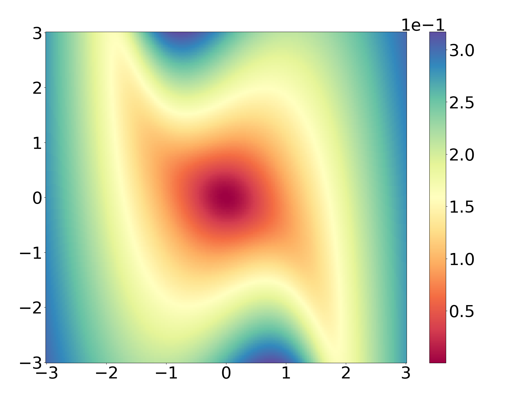
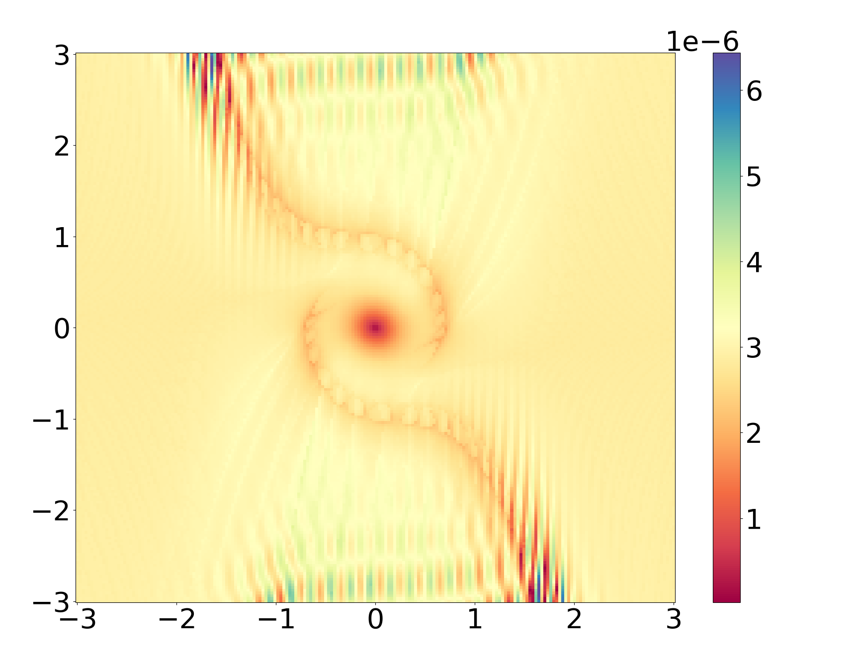
Figure 4: Left: The computed sum of squares solution for the nonlinear example. Right: The error between computed solution and the reference solution obtained by integrating over the trajectories.

We need to verify that the assumptions of Proposition 4.3 are satisfied. To do this, we first have to ensure that the linearized problem is locally stable around the origin. We have the decomposition

$$f(x_{1},x_{2})=A_{m}\begin{pmatrix}x_{1}\\ x_{2}\end{pmatrix}+\tilde{f}(x_{1},x_{2})=\begin{pmatrix}0&1\\ -1&\mu-\eta\end{pmatrix}\begin{pmatrix}x_{1}\\ x_{2}\end{pmatrix}+\tilde{f}(x_{1},x_{2})$$

where the eigenvalues of the matrix $A_{m}$ are given by

$$\lambda_{i}(A_{m})\mathrel{\mathop{\mathchar 58\relax}}=\frac{1}{2}\left(p\pm\sqrt{p^{2}-4}\right)\qquad\text{with}\;p\mathrel{\mathop{\mathchar 58\relax}}=\mu-\eta<0.$$

We immediately see that $\text{Re}(\lambda_{i}(A_{m}))<0$ for our choice of parameters and therefore the matrix is stable. As a reference solution, we approximate the Lyapunov function by integrating the cost along solution trajectories of the system. We use orthonormalized splines with $60$ nodes and degree $4$ for discretization and Gauss-Legendre quadrature of degree $4$ for integration on each subinterval. The rapid decay predicted in Lemma 3.10 can be seen in Fig. 3, along with the highly nonlinear eigenfunctions. The error between the reference solution and our method has a magnitude of around $10^{-5}$, as shown in Fig. 4. We attribute this error at least partially to the way we compute the reference solution.

6 Conclusion and outlook

In this paper, we presented a method for representing a Lyapunov function as the solution to an operator Lyapunov equation. We showed that the solution to this operator equation has a nuclear decomposition with rapidly decaying singular values which allows for a low-rank approximation. We demonstrated the feasibility of this approximation both theoretically and numerically.

Several aspects seem to be worth to be investigated further, one of them being the extension of our concepts to the case of (high-dimensional) nonlinear control problems which are often solved via a sequence of Lyapunov equations in the policy iteration. Moreover, we believe our results to be also applicable in the context of model order reduction where the linear structure of the infinite-dimensional system could be used for balanced truncation like techniques.

References

• [1] H. W. Alt, Linear functional analysis, Springer-Verlag London, 2016. An application-oriented introduction, Translated from the German edition by Robert Nürnberg.
• [2] A. C. Antoulas, D. C. Sorensen, and Y. Zhou, On the decay rate of the Hankel singular values and related issues, Systems & Control Letters, 46 (2002), pp. 323–342.
• [3] B. Azmi, D. Kalise, and K. Kunisch, Optimal feedback law recovery by gradient-augmented sparse polynomial regression, Journal of Machine Learning Research, 22 (2021), pp. 1–32.
• [4] P. Benner, J.-R. Li, and T. Penzl, Numerical solution of large-scale Lyapunov equations, Riccati equations, and linear-quadratic optimal control problems, Numerical Linear Algebra with Applications, 15 (2008), pp. 755–777.
• [5] P. Benner and J. Saak, Numerical solution of large and sparse continuous time algebraic matrix Riccati and Lyapunov equations: a state of the art survey, GAMM-Mitteilungen, 36 (2013), pp. 32–52.
• [6] S. L. Brunton, M. Budišić, E. Kaiser, and J. N. Kutz, Modern Koopman theory for dynamical systems, SIAM Review, 64 (2022), pp. 229–340.
• [7] M. Budišić, R. Mohr, and I. Mezić, Applied Koopmanism, Chaos: An Interdisciplinary Journal of Nonlinear Science, 22 (2012), p. 047510.
• [8] T. Carleman, Application de la théorie des équations intégrales linéaires aux systèmes d’équations différentielles non linéaires, Acta Mathematica, 59 (1932), pp. 63–87.
• [9] R. Curtain and H. Zwart, An Introduction to Infinite-Dimensional Linear Systems Theory, Springer, New York, 1995.
• [10] R. F. Curtain and A. J. Sasane, Compactness and nuclearity of the Hankel operator and internal stability of infinite-dimensional state linear systems, International Journal of Control, 74 (2001), pp. 1260–1270.
• [11] K. Engel and R. Nagel, A short course on operator semigroups, Springer, 2006.
• [12] L. C. Evans, Partial Differential Equations, American Mathematical Society, 1998.
• [13] G. Froyland, O. Junge, and P. Koltai, Estimating long term behavior of flows without trajectory integration: the infinitesimal generator approach, SIAM Journal on Numerical Analysis, 51 (2013), pp. 223–247.
• [14] D. Gottlieb and S. A. Orszag, Numerical Analysis of Spectral Methods, Society for Industrial and Applied Mathematics, 1977.
• [15] L. Grasedyck, Existence and computation of low Kronecker-rank approximations for large linear systems of tensor product structure, Computing, 72 (2004), pp. 247–265.
• [16] T. H. Gronwall, Note on the derivatives with respect to a parameter of the solutions of a system of differential equations, Annals of Mathematics, 20 (1919), pp. 292–296.
• [17] L. Grubisic and D. Kressner, On the eigenvalue decay of solutions to operator Lyapunov equations, Systems & Control Letters, 73 (2014), pp. 42–47.
• [18] S. Klus, F. Nüske, S. Peitz, J.-H. Niemann, C. Clementi, and C. Schütte, Data-driven approximation of the Koopman generator: Model reduction, system identification, and control, Physica D: Nonlinear Phenomena, 406 (2020), p. 132416.
• [19] B. O. Koopman, Hamiltonian systems and transformation in Hilbert space, Proceedings of the National Academy of Sciences, 17 (1931), pp. 315–318.
• [20] A. Lasota and M. C. Mackey, Chaos, Fractals, and Noise: Stochastic Aspects of Dynamics, Springer New York, New York, NY, 1994.
• [21] A. Mauroy and I. Mezić, Global stability analysis using the eigenfunctions of the Koopman operator, IEEE Transactions on Automatic Control, 61 (2016), pp. 3356–3369.
• [22] A. Mauroy, Y. Susuki, and I. Mezić, The Koopman operator in systems and control. Concepts, methodologies and applications, Cham: Springer, 2020.
• [23] I. Mezić, Spectral properties of dynamical systems, model reduction and decompositions, Nonlinear Dynamics, 41 (2005), pp. 309–325.
• [24] M. Opmeer, T. Reis, and W. Wollner, Finite-rank ADI iteration for operator Lyapunov equations, SIAM Journal on Control and Optimization, 51 (2013).
• [25] M. R. Opmeer, Decay of Hankel singular values of analytic control systems, Systems & Control Letters, 59 (2010), pp. 635–638.
• [26] M. R. Opmeer, Decay of singular values of the Gramians of infinite-dimensional systems, in 2015 European Control Conference (ECC), 2015, pp. 1183–1188.
• [27] M. R. Opmeer, Decay of singular values for infinite-dimensional systems with Gevrey regularity, Systems & Control Letters, 137 (2020), p. 104644.
• [28] T. Penzl, Eigenvalue decay bounds for solutions of Lyapunov equations: the symmetric case, Systems & Control Letters, 40 (2000), pp. 139–144.
• [29] W. Rudin, Principles of Mathematical Analysis, International series in pure and applied mathematics, McGraw-Hill, 1976.
• [30] W. Rudin, Real and complex analysis, McGraw-Hill, 1987.
• [31] J. M. A. Scherpen, Balancing for nonlinear systems, Systems & Control Letters, (1993), pp. 143–153.
• [32] V. Simoncini, A new iterative method for solving large-scale Lyapunov matrix equations, SIAM Journal on Scientific Computing, 29 (2007), pp. 1268–1288.
• [33]  , Computational methods for linear matrix equations, SIAM Review, 58 (2016), pp. 377–441.
• [34] R. K. Singh and J. S. Manhas, Composition operators on function spaces, vol. 179 of North-Holland Mathematics Studies, North-Holland Publishing Co., Amsterdam, 1993.
• [35] G. Szegö, Orthogonal Polynomials, vol. 23 of Colloquium Publications, American Mathematical Society, 1939.
• [36] M. Tucsnak and G. Weiss, Observation and Control for Operator Semigroups, Birkhäuser Basel, 2009.
• [37] W. Walter, Ordinary Differential Equations, Springer New York, 1998.