On Penalty-based Bilevel Gradient Descent Method

Abstract

Bilevel optimization enjoys a wide range of applications in hyper-parameter optimization, meta-learning and reinforcement learning. However, bilevel optimization problems are difficult to solve. Recent progress on scalable bilevel algorithms mainly focuses on bilevel optimization problems where the lower-level objective is either strongly convex or unconstrained. In this work, we tackle the bilevel problem through the lens of the penalty method. We show that under certain conditions, the penalty reformulation recovers the solutions of the original bilevel problem. Further, we propose the penalty-based bilevel gradient descent (PBGD) algorithm and establish its finite-time convergence for the constrained bilevel problem without lower-level strong convexity. Experiments showcase the efficiency of the proposed PBGD algorithm.

1 Introduction

Bilevel optimization plays an increasingly important role in machine learning (Liu et al., 2021a), image processing (Crockett and Fessler, 2022) and communications (Chen et al., 2023a). Specifically, in machine learning, it has a wide range of applications including hyper-parameter optimization (Maclaurin et al., 2015; Franceschi et al., 2018), meta-learning (Finn et al., 2017; Rajeswaran et al., 2019), reinforcement learning (Cheng et al., 2022) and adversarial learning (Jiang et al., 2021).

Define $f:\mathbb{R}^{d_{x}}\times\mathbb{R}^{d_{y}}\mapsto\mathbb{R}$ and $g:\mathbb{R}^{d_{x}}\times\mathbb{R}^{d_{y}}\mapsto\mathbb{R}$. We consider the following bilevel problem:

$$\mathcal{BP}:~{}~{}\min_{x,y}f(x,y)\,\,\,\,\,{\rm s.t.}\,\, x\in\mathcal{C},~{}y\in\mathcal{S}(x)\coloneqq\arg\min_{y\in\mathcal{U}(x)}g(x,y)$$

where $\mathcal{C}$, $\mathcal{U}(x)$ and $\mathcal{S}(x)$ are non-empty and closed sets given any $x\in\mathcal{C}$. We call $f$ and $g$ respectively as the upper-level and lower-level objective.

The bilevel optimization problem $\mathcal{BP}$ can be extremely difficult to solve due to the coupling between the upper-level and lower-level problems. Even for the simpler case where $g(x,\cdot)$ is strongly-convex, $\mathcal{U}(x)=\mathbb{R}^{d_{y}}$ and $\mathcal{C}=\mathbb{R}^{d_{x}}$, it was not until recently that the veil of an efficient method was partially lifted. Under the strong convexity of $g(x,\cdot)$, the lower-level solution set $\mathcal{S}(x)$ is a singleton. In this case, $\mathcal{BP}$ reduces to minimizing $f(x,\mathcal{S}(x))$, the gradient of which can be calculated with the implicit gradient (IG) method (Pedregosa, 2016; Ghadimi and Wang, 2018). It has been later shown by (Chen et al., 2021) that the IG method converges almost as fast as the gradient-descent method. However, existing IG methods cannot handle either the lower-level constraint $\mathcal{U}(x)$ or the non-strong convexity of $g(x,\cdot)$ due to the difficulty of computing the implicit gradient and thus can not be applied to more complicated bilevel problems.

To overcome the above challenges, recent work aims to develop gradient-based methods without lower-level strong convexity. A prominent branch of algorithms are based on the iterative differentiation method; see e.g., (Franceschi et al., 2017; Liu et al., 2021c). In this case, the lower-level solution set $\mathcal{S}(x)$ is replaced by the output of an iterative optimization algorithm that solves the lower-level problem (e.g., gradient descent (GD)) which allows for explicit differentiation. However, these methods are typically restricted to the unconstrained case since the lower-level algorithm with the projection operator is difficult to differentiate. Furthermore, the algorithm has high memory and computational costs when the number of lower-level iterations is large.

On the other hand, it is tempting to penalize certain optimality metric of the lower-level problem (e.g., $\|\nabla_{y}g(x,y)\|^{2}$) to the upper-level objective, leading to the single-level optimization problem. The high-level idea is that minimizing the optimality metric guarantees the lower-level optimality $y\in\mathcal{S}(x)$ and as long as the optimality metric admits simple gradient evaluation, the penalized objective can be optimized via gradient-based algorithms. However, as we will show in the next example, GD for a straightforward penalization mechanism may not lead to the desired solution of the original bilevel problems.

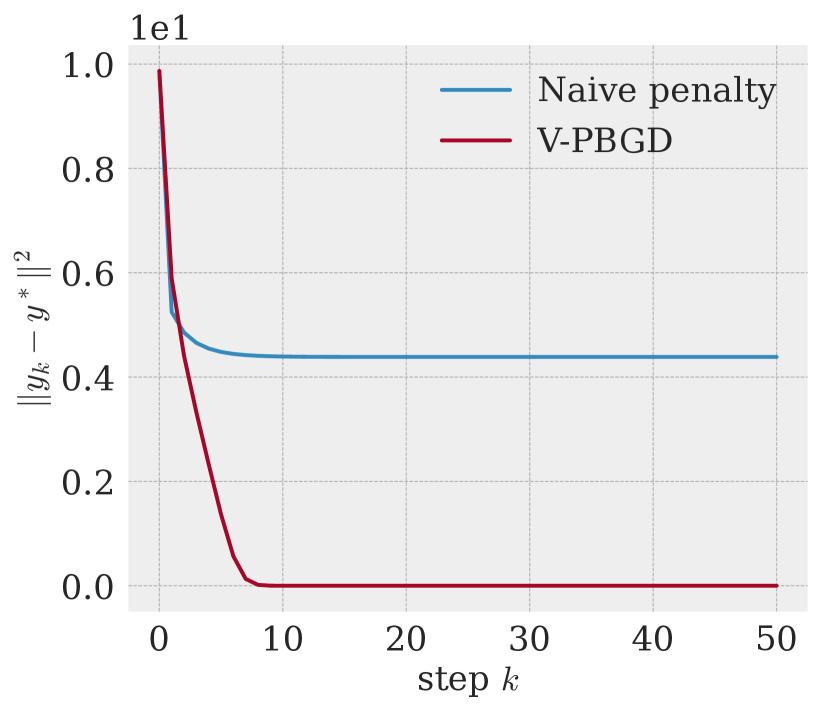
Figure 1: Naive penalty yields suboptimal points while the proposed algorithm finds the solution.

Example 1.

Consider the following special case of $\mathcal{BP}$:

$$\min_{x,y\in\mathbb{R}}~{}f(x,y)~{}\coloneqq\!\sin^{2}(y\!-\!\frac{2\pi}{3})\,\,\,\,{\rm s.t.}~{}~{}~{}~{}y\in\arg\min_{y\in\mathbb{R}}g(x,y)\coloneqq y^{2}\!+\!2\sin^{2}y.$$ (1.1)

The only solution of (1.1) is $y^{*}\!=\!0$. In this example, it can be checked that $\|\nabla_{y}g(x,y)\|^{2}=0$ if only if $y\in\arg\min_{y\in\mathbb{R}}g(x,y)$ and thus $\|\nabla_{y}g(x,y)\|^{2}=0$ is a lower-level optimality metric. Penalizing $f(x,y)$ with the penalty function $\|\nabla_{y}g(x,y)\|^{2}$ and a penalty constant $\gamma>0$ gives $\min f(x,y)+\gamma(y+\sin(2y))^{2}$. For any $\gamma$, $y=\frac{2\pi}{3}$ is a local solution of the penalized problem while is is neither a global solution nor a local solution of the original problem (1.1).

In Figure 1, we show that in Example 1 the naive penalty method, i.e. solving $\min f(x,y)+\gamma(y+\sin(2y))^{2}$, can get stuck at sub-optimal points. To tackle such issues, it is crucial to study the relation between the bilevel problem and its penalized problem. Specifically, what impact do different penalty terms, penalization constants and problem properties have on this relation? Through studying this relation, we aim to develop an efficient penalty-based bilevel gradient descent method for $\mathcal{BP}$.

Our contributions. In this work, we will first consider the following penalty reformulation of $\mathcal{BP}$, given by

$$\mathcal{BP}_{\gamma p}:\min_{x,y}f(x,y)+\gamma p(x,y),~{}~{}~{}{\rm s.t.}~{}~{}~{}x\in\mathcal{C},~{}y\in\mathcal{U}(x)$$

where $p(x,y)$ is a certain penalty term that will be specified in Section 3. Our first result shows that under certain generic conditions on $g(x,y)$, one can recover approximate global (local) solutions of $\mathcal{BP}$ by solving $\mathcal{BP}_{\gamma p}$ globally (locally). Further, we show that these generic conditions hold without the strong convexity of $g(x,\cdot)$. Then we propose a penalized bilevel GD (PBGD) method and establish its finite-time convergence when the lower-level is unconstrained (e.g., $\mathcal{U}(x)\!=\!\mathbb{R}^{d_{y}}$) or the constraint set $\mathcal{U}(x)\!=\!\mathcal{U}$ is a compact convex set. We summarize the convergence results of our algorithm and compare them with several related works in Table 1. Finally, we empirically showcase the performance, computation and memory efficiency of the proposed algorithm in comparison with several competitive baselines.

	V-PBGD (ours)	BOME	IAPTT-GM	AiPOD
Upper-level constraint	✓	✗	✓	✓
Lower-level constraint	$\mathcal{U}(x)\!=\!\mathbb{R}^{d_{x}}\text{ or }\mathcal{U}$	✗	$\mathcal{U}(x)\!=\!\mathcal{U}$	equality constraint
Lower-level non-strongly-convex	✓	✓	✓	✗
Non-singleton $\mathcal{S}(x)$	✓	✗	✓	✗
First-order	✓	✓	✗	✗
Convergence	finite-time	finite-time	asymptotic	finite-time

Table 1: Comparison of this work (V-PBGD) and IAPTT-GM (Liu et al., 2021c), BOME (Ye et al., 2022), AiPOD (Xiao et al., 2023). In the table, $\mathcal{U}$ is a convex compact set.

	Section 3	Section 4	Section 5
Upper-level constraint	$\mathcal{C}$ closed and convex
Lower-level Constraint	$\mathcal{U}(x)=\mathbb{R}^{d_{y}}$	$\mathcal{U}(x)=\mathcal{U}$ is closed convex	$\mathcal{U}(x)=\mathbb{R}^{d_{y}}$
$\text{Assumption}^{\dagger}$ on $f$	$f(x,\cdot)$ is Lipschitz-continuous
$\text{Assumption}^{\dagger}$ on $g(x,\cdot)$	$\text{PL}^{\ddagger}$	$\text{QG+convex/EB}^{\ddagger}$	$\text{PL}^{\ddagger},~{}\|\nabla_{y}g(x,\cdot)\|$ convex
Constant $\gamma$	$\Omega(\epsilon^{-0.5})$	$\Omega(\epsilon^{-0.5})$	$\Omega(1)$
Iteration complexity	$\mathcal{O}(\epsilon^{-1.5})$	$\mathcal{O}(\epsilon^{-1.5})$	$\mathcal{O}(\epsilon^{-1})$

Table 2: Comparison of the main theorems in this paper. Here $\epsilon$ is the accuracy. ^†The Lipschitz-smooth assumption on $f,g$ are neglected in this table; ^‡PL short for Polyak-Łojasiewicz, QG short for quadratic growth, EB short for error bound. These notions will be defined in each section.

1.1 Related works

The bilevel optimization problem can be dated back to (Stackelberg, 1952). Recently, the gradient-based bilevel optimization methods have gained growing popularity in the machine learning area; see, e.g., (Sabach and Shtern, 2017; Franceschi et al., 2018; Liu et al., 2020). A branch of gradient-based methods belongs to the IG method (Pedregosa, 2016). The finite-time convergence was first established in (Ghadimi and Wang, 2018) for the unconstrained strongly-convex lower-level problem. Later, the convergence was improved in (Hong et al., 2023; Ji et al., 2021; Chen et al., 2022, 2021; Khanduri et al., 2021; Shen and Chen, 2022; Li et al., 2022; Sow et al., 2022). Recent works extend IG to constrained strongly-convex lower-level problems; see, e.g., the equality-constrained IG method (Xiao et al., 2023) and a 2nd-derivative-free approach (Giovannelli et al., 2022).

Another branch of methods is based on the iterative differentiation (ITD) methods (Maclaurin et al., 2015; Franceschi et al., 2017; Nichol et al., 2018; Shaban et al., 2019). Later, (Liu et al., 2021c) proposes an ITD method with initialization optimization and shows asymptotic convergence. Another work (Liu et al., 2022b) develops an ITD method where each lower-level iteration uses a combination of upper-level and lower-level gradients. Recently, the iterative differentiation of non-smooth lower-level algorithms has been studied in (Bolte et al., 2022). The ITD methods generally lack finite-time guarantee unless restrictive assumptions are made for the iteration mapping (Grazzi et al., 2020; Ji et al., 2022).

Recently, bilevel optimization methods have also been studied in distributed learning (Tarzanagh et al., 2022; Lu et al., 2022; Yang et al., 2022), corset selection (Zhou et al., 2022), overparametrized setting (Vicol et al., 2022), multi-block min-max (Hu et al., 2022), game theory (Arbel and Mairal, 2022) and several acceleration methods have been proposed (Huang et al., 2022; Dagréou et al., 2022). The works (Liu et al., 2021b) and (Mehra and Hamm, 2021) propose penalty-based methods respectively with log-barrier and gradient norm penalty, and establish their asymptotic convergence. Another work (Gao et al., 2022) develops a method based on the difference-of-convex algorithm. In preparing our final version, a concurrent work (Chen et al., 2023b) studies the bilevel problem with convex lower-level objectives and proposes a zeroth-order optimization method with finite-time convergence to the Goldstein stationary point. Another concurrent work (Lu and Mei, 2023) proposes a penalty method for the bilevel problem with a convex lower-level objective $g(x,\cdot)$. It shows convergence to a weak $KKT$ point of the bilevel problem while does not study the relation between the bilevel problem and its penalized problem.

The relation between the bilevel problem and its penalty reformulation has been first studied in (Ye et al., 1997) under the calmness condition paired with other conditions such as the 2-Hölder continuity, which are difficult to satisfy. A recent work (Ye et al., 2022) proposes a novel first-order method that is termed BOME. By assuming the constant rank constraint qualification (CRCQ), (Ye et al., 2022) shows convergence of BOME to a KKT point of the bilevel problem. However, it is unclear when CRCQ can be satisfied and the convergence relies on restrictive assumptions like the uniform boundedness of $\|\nabla g\|$, $\|\nabla f\|$, $|f|$ and $|g|$. It is also difficult to argue when the KKT point is a solution of the bilevel problem under lower-level non-convexity.

Notations. We use $\|\cdot\|$ to denote the $l^{2}$-norm. Given $r>0$ and $z\in\mathbb{R}^{d}$, define $\mathcal{N}(z,r)\coloneqq\{z^{\prime}\in\mathbb{R}^{d}:\|z-z^{\prime}\|\leq r\}$. Given vectors $x$ and $y$, we use $(x,y)$ to indicate the concatenated vector of $x,y$. Given a non-empty closed set $\mathcal{S}\subseteq\mathbb{R}^{d}$, define the distance of $y\in\mathbb{R}^{d}$ to the set $\mathcal{S}$ as $d_{\mathcal{S}}(y)\coloneqq\min_{y^{\prime}\in\mathcal{S}}\|y-y^{\prime}\|$. We use $\operatorname{Proj}_{\mathcal{Z}}$ to denote the projection to the set $\mathcal{Z}$.

2 Penalty Reformulation of Bilevel Problems

In this section, we study the relation between the solutions of the bilevel problem $\mathcal{BP}$ and those of its penalty reformulation $\mathcal{BP}_{\gamma p}$. Since $\mathcal{S}(x)$ is closed, $y\in\mathcal{S}(x)$ is equivalent to $d_{\mathcal{S}(x)}(y)=0$. We therefore rewrite $\mathcal{BP}$ as

$$\min_{x,y}f(x,y)\,\,\,\,\,{\rm s.t.}\,\, x\in\mathcal{C},~{}d^{2}_{\mathcal{S}(x)}(y)=0.$$ (2.1)

The squared distance $d^{2}_{\mathcal{S}(x)}(y)$ is non-differentiable, and thus penalizing it to the upper-level objective is computationally-intractable. Instead, we consider its upper bounds defined as follows.

Definition 1 (Squared-distance bound function).

A function $p:\mathbb{R}^{d_{x}}\times\mathbb{R}^{d_{y}}\mapsto\mathbb{R}$ is a $\rho$-squared-distance-bound if there exists $\rho>0$ such that for any $x\in\mathcal{C},y\in\mathcal{U}(x)$, it holds

$$p(x,y)\geq 0,~{}\rho p(x,y)\geq d_{\mathcal{S}(x)}^{2}(y)$$ (2.2a)

$$p(x,y)=0~{}\text{ if and only if }~{}d_{\mathcal{S}(x)}(y)=0.$$ (2.2b)

Suppose $p(x,y)$ is a squared-distance bound function. Given $\epsilon\!>\!0$, we define the following $\epsilon$-approximate problem of the original bilevel problem $\mathcal{BP}$:

$$\mathcal{BP}_{\epsilon}:~{}\min_{x,y}f(x,y)\,\,\,\,\,{\rm s.t.}\,\, x\in\mathcal{C},~{}y\in\mathcal{U}(x),~{}p(x,y)\leq\epsilon.$$

It is clear that $\mathcal{BP}_{\epsilon}$ with $\epsilon=0$ recovers $\mathcal{BP}$. For $\epsilon>0$, $\mathcal{BP}_{\epsilon}$ is an $\epsilon$-approximate problem of $\mathcal{BP}$ since $p(x,y)$ is an upper bound of $d_{\mathcal{S}(x)}^{2}(y)$ and is smaller than $\epsilon$.

We start by considering the relation between the global solutions of $\mathcal{BP}_{\epsilon}$ and $\mathcal{BP}_{\gamma p}$. Before we introduce the theorem, we first give the following definition and assumption.

Definition 2 (Lipschitz continuity).

Given $L>0$, a function $\mathcal{L}:\mathbb{R}^{d}\mapsto\mathbb{R}^{d^{\prime}}$ is said to be $L$-Lipschitz-continuous on $\mathcal{X}\subseteq\mathbb{R}^{d}$ if it holds for any $x,x^{\prime}\in\mathcal{X}$ that $\|\mathcal{L}(x)-\mathcal{L}(x^{\prime})\|\leq L\|x-x^{\prime}\|$. A function $\mathcal{L}$ is said to be $L$-Lipschitz-smooth if its gradient is $L$-Lipschitz-continuous.

Assumption 1.

There exists $L\!>\!0$ that given any $x\in\mathcal{C}$, $f(x,\cdot)$ is $L$-Lipschitz continuous on $\mathcal{U}(x)$.

The above assumption is standard and has been made in several other works studying bilevel optimization; see, e.g., (Ghadimi and Wang, 2018; Chen et al., 2021, 2023b). In order to establish relation between the solutions of $\mathcal{BP}_{\gamma p}$ and those of $\mathcal{BP}$, a crucial step is to guarantee that $(x_{\gamma},y_{\gamma})$, which is a solution of $\mathcal{BP}_{\gamma p}$, is feasible for $\mathcal{BP}_{\epsilon}$, i.e., to guarantee $p(x_{\gamma},y_{\gamma})$ is small. Under Assumption 1, the growth of $f(x_{\gamma},\cdot)$ is controlled. Then an important intuition is that increasing $\gamma$ in $\mathcal{BP}_{\gamma p}$ likely makes $p(x_{\gamma},\cdot)$ more dominant, and thus decreases $p(x_{\gamma},y_{\gamma})$. With this intuition, we introduce the theorem as follows.

Theorem 1 (Relation on global solutions).

Assume $p(x,y)$ is a $\rho$-squared-distance-bound function and Assumption 1 holds. Given any $\epsilon_{1}>0$, any global solution of $\mathcal{BP}$ is an $\epsilon_{1}$-global-minimum point of $\mathcal{BP}_{\gamma p}$ with any $\gamma\geq\gamma^{*}=\frac{L^{2}\rho}{4}\epsilon_{1}^{-1}$. Conversely, given $\epsilon_{2}\geq 0$, if $(x_{\gamma},y_{\gamma})$ achieves $\epsilon_{2}$-global-minimum of $\mathcal{BP}_{\gamma p}$ with $\gamma>\gamma^{*}$, $(x_{\gamma},y_{\gamma})$ is the global solution of $\mathcal{BP}_{\epsilon_{\gamma}}$ with some $\epsilon_{\gamma}\leq(\epsilon_{1}\!+\!\epsilon_{2})/(\gamma\!-\!\gamma^{*})$.

The proof of Theorem 1 can be found in Appendix A.1. In Example 1, $\|\nabla_{y}g(x,y)\|^{2}$ is a squared-distance-bound and the above theorem regarding global solutions holds. However, as illustrated in Example 1, a penalized problem with any $\gamma>0$ always admits a local solution that is meaningless to the original problem. In fact, the relationship between local solutions is more intricate than that between global solutions. Nevertheless, we prove in the following theorem that under some verifiable conditions, the local solutions of $\mathcal{BP}_{\gamma p}$ are local solutions of the $\mathcal{BP}_{\epsilon}$.

Theorem 2 (Relation on local solutions).

Assume $p(x,\cdot)$ is continuous given any $x\in\mathcal{C}$ and $p(x,y)$ is $\rho$-squared-distance-bound function. Given $\gamma>0$, let $(x_{\gamma},y_{\gamma})$ be a local solution of $\mathcal{BP}_{\gamma p}$ on $\mathcal{N}((x_{\gamma},y_{\gamma}),r)$. Assume $f(x_{\gamma},\cdot)$ is $L$-Lipschitz-continuous on $\mathcal{N}(y_{\gamma},r)$. Assume either one of the following is true:

1. There exists $\bar{y}\in\mathcal{N}(y_{\gamma},r)$ such that $\bar{y}\in\mathcal{U}(x_{\gamma})$ and $p(x_{\gamma},\bar{y})\leq\epsilon$ for some $\epsilon\geq 0$. Define $\bar{\epsilon}_{\gamma}=\frac{L^{2}\rho}{\gamma^{2}}\!+\!2\epsilon$.

2. The set $\mathcal{U}(x_{\gamma})$ is convex and the function $p(x_{\gamma},\cdot)$ is convex. Define $\bar{\epsilon}_{\gamma}=\frac{L^{2}\rho}{\gamma^{2}}$.

Then $(x_{\gamma},y_{\gamma})$ is a local solution of $\mathcal{BP}_{\epsilon_{\gamma}}$ with $\epsilon_{\gamma}\leq\bar{\epsilon}_{\gamma}$.

The proof of Theorem 2 can be found in Appendix A.2. We provide a remark below.

Remark 1 (Intuition of the conditions).

In (i) of Theorem 2, we need an approximate global minimizer of $p(x_{\gamma},\cdot)$; and, in (ii), we assume $p(x_{\gamma},\cdot)$ is convex. Loosely speaking, these conditions essentially require $\min_{\mathcal{U}(x)}p(x,\cdot)$ to be globally solvable. Such a requirement is natural since finding a feasible point in $\mathcal{S}(x)$ is possible only if one can solve for $p(x,\cdot)=0$ on $\mathcal{U}(x)$. While they appear to be abstract, we will show how Conditions (i) and (ii) in Theorem 2 can be verified in the following sections.

3 Solving Bilevel Problems with Non-convex Lower-level Objectives

To develop algorithms with non-asymptotic convergence, we consider $\mathcal{BP}$ with unconstrained lower-level problem ($\mathcal{U}(x)\!=\!\mathbb{R}^{d_{y}}$ in this case), given by

where we assume $\mathcal{C}$ is a closed convex set and $f,g$ are continuously differentiable.

3.1 Candidate penalty terms

Following Section 2, to reformulate $\mathcal{UP}$, we first seek a squared-distance bound function $p$ that satisfies Definition 1. For a non-convex function $g(x,\cdot)$, an interesting property is the Polyak-Łojasiewicz (PL) inequality which is defined in the next assumption.

Assumption 2 (Polyak-Lojasiewicz function).

The lower-level function $g(x,\cdot)$ satisfies the $\frac{1}{\mu}$-PL inequality; that is, there exists $\mu>0$ such that given any $x\in\mathcal{C}$, it holds for any $y\in\mathbb{R}^{d_{y}}$ that

$$\|\nabla_{y}g(x,y)\|^{2}\geq\frac{1}{\mu}(g(x,y)-v(x))~{}\text{ where $v(x)\coloneqq\min_{y\in\mathbb{R}^{d_{y}}}g(x,y)$.}$$ (3.1)

In reinforcement learning, it has been proven in (Mei et al., 2020, Lemma 8&9) that the non-convex discounted return objective satisfies the PL inequality under certain parameterization. Moreover, recent studies found that over-parameterized neural networks can lead to losses that satisfy the PL inequality (Liu et al., 2022a).

Under the PL inequality, we consider the following potential penalty functions:

The next lemma shows that the above penalty functions are squared-distance bound functions.

Lemma 1.

Consider the following assumptions:

1. Suppose Assumption 2 holds, and there exists $L_{g}$ such that $\forall x\in\mathcal{C}$, $g(x,\cdot)$ is $L_{g}$-Lipschitz-smooth.

2. Suppose Assumption 2 holds with modulus $\frac{1}{\sqrt{\mu}}$.

Then (3.2a) and (3.2b) are $\mu$-squared-distance-bound functions respectively under (i) and (ii).

The proof of Lemma 1 can be found in Appendix B.1.

3.2 Penalty reformulation

Given a squared-distance bound $p(x,y)$ and constants $\gamma\!>\!0$ and $\epsilon>0$, define the penalized problem and the $\epsilon$-approximate bilevel problem of $\mathcal{UP}$ respectively as

$$\mathcal{UP}_{\gamma p}:~{} \min_{x,y}~{}F_{\gamma}(x,y)\,\coloneqq f(x,y)+\gamma p(x,y)$$

$${\rm s.t.}~{}\,\,x\in\mathcal{C}.$$

$$\mathcal{UP}_{\epsilon}:~{} \min_{x,y}~{}f(x,y)$$

$${\rm s.t.}~{}\,\,x\in\mathcal{C},~{}p(x,y)\leq\epsilon.$$

It remains to show that the solutions of $\mathcal{UP}_{\gamma p}$ are meaningful to $\mathcal{UP}$. Starting with the global solutions, we give the following proposition.

Proposition 1 (Relation on global solutions).

Assume Assumption 1 and either of the following holds:

1. Condition (i) Lemma 1 hold; and, choose $p(x,y)=g(x,y)-v(x)$.

2. Condition (ii) in Lemma 1 holds; and, choose $p(x,y)=\|\nabla_{y}g(x,y)\|^{2}$.

Suppose $\gamma\geq L\sqrt{\mu\delta^{-1}}$ with some $\delta>0$. Let $(x_{\gamma},y_{\gamma})$ be a global solution of $\mathcal{UP}_{\gamma p}$. Then $(x_{\gamma},y_{\gamma})$ is a global solution of $\mathcal{UP}_{\epsilon_{\gamma}}$ with $\epsilon_{\gamma}\leq\delta$.

Proposition 1 follows directly from Theorem 1 with $\epsilon_{1}=L\sqrt{\rho\delta}/2$, $\gamma\geq 2\gamma^{*}=L\sqrt{\mu\delta^{-1}}$ and $\epsilon_{2}=0$. By Proposition 1, the global solution of $\mathcal{UP}_{\gamma p}$ solves an approximate bilevel problem of $\mathcal{UP}$. However, since $\mathcal{UP}_{\gamma p}$ is generally non-convex, it is also important to consider the local solutions. Following Theorem 2, the next proposition captures the relation on the local solutions.

Proposition 2 (Relation on local solutions).

Assume Assumption 1 and either of the following holds:

1. Condition (i) in Lemma 1 holds; with some $\delta>0$, choose

   $$p(x,y)=g(x,y)-v(x)\quad{\rm and}\quad\gamma\geq L\sqrt{3\mu\delta^{-1}}.$$

2. Condition (ii) in Lemma 1 holds; with some $\delta>0$, choose

   $$p(x,y)=\|\nabla_{y}g(x,y)\|^{2}\quad{\rm and}\quad\gamma\geq\max\{L\sqrt{2\mu\delta^{-1}},L\sigma^{-1}\sqrt{\delta^{-1}}\}$$

   where $\sigma>0$ is the lower-bound of the singular values of $\nabla_{yy}g(x,y)$ on $\{(x,y)\!\in\!\mathcal{C}\!\times\!\mathbb{R}^{d_{y}}\!:y\notin\!\mathcal{S}(x)\}$.

If $(x_{\gamma},y_{\gamma})$ is a local solution of $\mathcal{UP}_{\gamma p}$, then it is a local solution of $\mathcal{UP}_{\epsilon_{\gamma}}\!$ with some $\epsilon_{\gamma}\!\leq\!\delta$.

The proof of Proposition 2 can be found in Appendix B.2. Proposition 2 explains the observations in Figure 1 and Example 1. The failing point $y=\frac{2\pi}{3}$ mentioned in Example 1 yields $\nabla_{yy}g(x,y)=0$ which violates (b) in Proposition 2. It can be checked that (a) of Proposition 2 holds in Example 1.

Propositions 1 and 2 suggest $\gamma=\Omega(\delta^{-0.5})$ to achieve $\epsilon_{\gamma}\leq\delta$. Next we show this is tight.

Corollary 1.

In Proposition 1 or 2, to guarantee $\epsilon_{\gamma}=\mathcal{O}(\delta)$, the lower-bound on the penalty constant $\gamma=\Omega(\delta^{-0.5})$ is tight.

Proof.

Consider the following special case of $\mathcal{UP}$:

$$\min_{y\in\mathbb{R}}f(x,y)=y,~{}~{}~{}{\rm s.t.}~{}~{}~{}y\in\arg\min_{y\in\mathbb{R}}g(x,y)=y^{2}.$$ (3.3)

In the example, the two penalty terms $\frac{1}{4}\|\nabla_{y}g(x,y)\|^{2}$ and $g(x,y)-v(x)$ coincide to be $p(x,y)=y^{2}$. In this case, solutions of $\mathcal{UP}$ and $\mathcal{UP}_{\gamma p}$ are respectively $0$ and $-\frac{1}{2\gamma}$. Thus $-\frac{1}{2\gamma}$ is a solution of $\mathcal{CP}_{\epsilon_{\gamma}}$ with $\epsilon_{\gamma}=1/(4\gamma^{2})$. To ensure $\epsilon_{\gamma}=\mathcal{O}(\delta)$, $\gamma=\Omega(\delta^{-0.5})$ is required in this example. Then the proof is complete by the fact that the assumptions in Proposition 1 and 2 hold in this example. ∎

Propositions 1 and 2 imply that $\mathcal{UP}$ and $\mathcal{UP}_{\gamma p}$ are related in the sense that one can globally/locally solve an approximate bilevel problem of $\mathcal{UP}$ by globally/locally solving the penalized problem $\mathcal{UP}_{\gamma p}$ instead. A natural approach to solving the penalized problem is the projected gradient method. At each iteration $k$, we assume access to $h_{k}$ which is either $\nabla p(x_{k},y_{k})$ or its estimate if $\nabla p$ cannot be exactly evaluated. We then update $(x_{k},y_{k})$ with $\nabla F_{\gamma}(x_{k},y_{k})$ evaluated using $h_{k}$. The process is summarized in Algorithm 1.

Algorithm 1 PBGD: Penalized bilevel GD

1:  Select $(x_{1},y_{1})\in\mathcal{Z}\coloneqq\mathcal{C}\times\mathcal{U}(x)$. Select step size $\alpha$, penalty constant $\gamma$ and iteration number $K$.

2:  for $k=1$ to $K$ do

3:     Compute $h_{k}=\nabla p(x_{k},y_{k})$ or its estimate.

4:     $(x_{k+1},y_{k+1})=\operatorname{Proj}_{\mathcal{Z}}\Big{(}(x_{k},y_{k})-\alpha\big{(}\nabla f(x_{k},y_{k})+\gamma h_{k}\big{)}\Big{)}$.

5:  end for

When $p(x,y)=\|\nabla_{y}g(x,y)\|^{2}$, $\nabla p(x,y)$ can be exactly evaluated. In this case, Algorithm 1 is a standard projected gradient method and the convergence property directly follows from the existing literature. In the next subsection, we focus on the other penalty function $p(x,y)=g(x,y)-v(x)$ and discuss when $\mathcal{UP}_{\gamma p}$ can be efficiently solved.

3.3 PBGD with function value gap

We consider solving $\mathcal{UP}_{\gamma p}$ with $p(x,y)$ chosen as the function value gap (3.2a). To solve $\mathcal{UP}_{\gamma p}$ with the gradient-based method, the obstacle is that $\nabla p(x,y)$ requires $\nabla v(x)$. On one hand, $v(x)$ is not necessarily smooth. Even if $v(x)$ is differentiable, $\nabla v(x)\neq\nabla_{x}g(x,y^{*})~{}\text{in general, where }y^{*}\in\mathcal{S}(x)$. However, it is possible to compute $\nabla v(x)$ efficiently under some relatively mild conditions.

Lemma 2 ((Nouiehed et al., 2019, Lemma A.5)).

Assume Assumption 2 holds, and $g$ is $L_{g}$-Lipschitz-smooth. Then $\nabla v(x)=\nabla_{x}g(x,y^{*})$ for any $y^{*}\in\mathcal{S}(x)$, and $v(x)$ is $(L_{g}\!+\!L_{g}^{2}\mu)$-Lipschitz-smooth.

Under the conditions in Lemma 2, $\nabla v(x)$ can be evaluated directly at any optimal solution of the lower-level problem. This suggests one find a lower-level optimal solution $y^{*}\in\mathcal{S}(x)$, and evaluate the penalized gradient $\nabla F_{\gamma}(x,y)$ with $\nabla v(x)=\nabla_{x}g(x,y^{*})$. Following this idea, given outer iteration $k$ and $x_{k}$, we run $T_{k}$ steps of inner GD update to solve the lower-level problem:

$$\omega_{t+1}^{(k)} =\omega_{t}^{(k)}-\beta\nabla_{y}g(x_{k},\omega_{t}^{(k)}),~{}t=1,\dots,T_{k}$$ (3.4a)

where $$\omega_{1}^{(k)}=y_{k} \hat{y}_{k}=\omega_{T_{k}+1}^{(t)} \nabla F_{\gamma}(x_{k},y_{k}) \hat{y}_{k} (x_{k},y_{k})$$. Update (3.4a) yields an approximate lower-level solution . Then we can approximate with and update via:

$$(x_{k+1},y_{k+1}) =\operatorname{Proj}_{\mathcal{Z}}\Big{(}(x_{k},y_{k})-\alpha\big{(}\nabla f(x_{k},y_{k})+\gamma(\nabla g(x_{k},y_{k})-\overline{\nabla}_{x}g(x_{k},\hat{y}_{k})\big{)}\Big{)}$$ (3.4b)

where $\mathcal{Z}=\mathcal{C}\times\mathbb{R}^{d_{y}}$ and $\overline{\nabla}_{x}g(x,y)\coloneqq(\nabla_{x}g(x,y),\mathbf{0})$ with $\mathbf{0}\in\mathbb{R}^{d_{y}}$. The update is summarized in Algorithm 2, which is a function value gap-based special case of PBGD (Algorithm 1) with $h_{k}=\nabla g(x_{k},y_{k})-\overline{\nabla}_{x}g(x_{k},\hat{y}_{k})$.

Notice that only first-order information is required in update (3.4), which is in contrast to the implicit gradient methods or some iterative differentiation methods where higher-order derivatives are required; see, e.g., (Ghadimi and Wang, 2018; Franceschi et al., 2017; Liu et al., 2021c). In modern machine learning applications, this could substantially save computational cost since the dimension of parameter is often large, making higher-order derivatives particularly costly.

Algorithm 2 V-PBGD: Function value gap based PBGD

1:  Select $(x_{1},y_{1})\in\mathcal{Z}=\mathcal{C}\times\mathbb{R}^{d_{y}}$. Select step sizes $\alpha,\beta$, constant $\gamma$, iteration numbers $T_{k}$ and $K$.

2:  for $k=1$ to $K$ do

3:     Obtain $\hat{y}_{k}=\omega_{T_{k}+1}^{(k)}$ following (3.4a).

4:     Update $(x_{k},y_{k})$ following (3.4b).

5:  end for

3.4 Analysis of PBGD with function value gap

We first introduce the following regularity assumption commonly made in the convergence analysis of the gradient-based bilevel optimization methods (Chen et al., 2021; Grazzi et al., 2020).

Assumption 3 (smoothness).

There exist constants $L_{f}$ and $L_{g}$ such that $f(x,y)$ and $g(x,y)$ are respectively $L_{f}$-Lipschitz-smooth and $L_{g}$-Lipschitz-smooth in $(x,y)$.

Define the projected gradient of $\mathcal{UP}_{\gamma p}$ at $(x_{k},y_{k})\in\mathcal{Z}$ as

$$G_{\gamma}(x_{k},y_{k})\coloneqq\frac{1}{\alpha}\big{(}(x_{k},y_{k})-(\bar{x}_{k+1},\bar{y}_{k+1})\big{)},$$ (3.5)

where $(\bar{x}_{k+1},\bar{y}_{k+1})\coloneqq\operatorname{Proj}_{\mathcal{Z}}((x_{k},y_{k})-\alpha\nabla F_{\gamma}(x_{k},y_{k}))$. This definition (3.5) is commonly used as the convergence metric for the projected gradient methods. It is known that given a convex $\mathcal{Z}$, $G_{\gamma}(x,y)\!=\!0$ if and only if $(x,y)$ is a stationary point of $\mathcal{UP}_{\gamma p}$ (Ghadimi et al., 2016). We provide the following theorem on the convergence of V-PBGD.

Theorem 3.

Consider V-PBGD (Algorithm 2). Suppose Assumption 1,2 and 3 hold. Select $\omega_{1}^{(k)}=y_{k}$ and

$$\alpha\in(0,(L_{f}+\gamma(2L_{g}+L_{g}^{2}\mu))^{-1}],~{}\beta\in(0,L_{g}^{-1}],~{}\gamma\geq L\sqrt{3\mu\delta^{-1}},~{}T_{k}=\Omega(\log(\alpha k)).$$

i) With $C_{f}\!=\!\inf_{(x,y)\in\mathcal{Z}}f(x,y)$, it holds that

$$\frac{1}{K}\sum_{k=1}^{K}\|G_{\gamma}(x_{k},y_{k})\|^{2}\leq\frac{18\big{(}F_{\gamma}(x_{1},y_{1})-C_{f}\big{)}}{\alpha K}+\frac{10L^{2}L_{g}^{2}}{K}.$$

ii) Suppose $\lim_{k\rightarrow\infty}(x_{k},y_{k})=(x^{*},y^{*})$, then $(x^{*},y^{*})$ is a stationary point of $\mathcal{UP}_{\gamma p}$. If $(x^{*},y^{*})$ is a local/global solution of $\mathcal{UP}_{\gamma p}$, it is a local/global solution of $\mathcal{UP}_{\epsilon_{\gamma}}$ with some $\epsilon_{\gamma}\leq\delta$.

The proof of Theorem 3 can be found in Appendix B.3. Theorem 3 implies an iteration complexity of $\widetilde{\mathcal{O}}(\gamma\epsilon^{-1})$ to find an $\epsilon$-stationary-point of $\mathcal{UP}_{\gamma p}$. This recovers the iteration complexity of the projected GD method (Nesterov, 2013) with a smoothness constant of $\Theta(\gamma)$. If we choose $\delta=\epsilon$, then we get an iteration complexity of $\widetilde{\mathcal{O}}(\epsilon^{-1.5})$. In (ii), under no stronger conditions needed for the projected GD method to yield meaningful solutions, the V-PBGD algorithm finds a local/global solution of the approximate $\mathcal{UP}$.

In addition to the deterministic PBGD algorithm, a stochastic version of the V-PBGD algorithm and its convergence analysis are provided in Appendix B.4.

4 Solving Bilevel Problems with Lower-level Constraints

In the previous section, we have introduced the PBGD method to solve a class of non-convex bilevel problems with only upper-level constraints. When the lower-level constraints are involved, it becomes more difficult to develop a gradient-based algorithm with finite-time guarantees.

In this section, under assumptions on the lower-level objective that are weaker than the commonly used strong-convexity assumption, we propose an algorithm with finite-time convergence guarantee. Specifically, consider the special case of $\mathcal{BP}$ with $\mathcal{U}(x)=\mathcal{U}$:

where we assume $\mathcal{C}$ and $\mathcal{U}$ are convex and compact in this section.

4.1 Penalty reformulation

Following Section 2, we seek to reformulate $\mathcal{CP}$ with a suitable penalty function $p(x,y)$. In this section, we consider choosing $p(x,y)$ as the lower-level function value gap $g(x,y)-v(x)$ where $v(x)\coloneqq\min_{y\in\mathcal{U}}g(x,y)$. We first list some assumptions that will be repeatedly used in this section.

Assumption 4.

Consider the following conditions:

1. There exists $\mu>0$ such that $\forall x\in\mathcal{C}$, $g(x,\cdot)$ has $\frac{1}{\mu}$-quadratic-growth, that is, $\forall y\in\mathcal{U}$, it holds that

   $$g(x,y)-v(x)\geq\frac{1}{\mu}d^{2}_{\mathcal{S}(x)}(y).$$

2. There exists $\bar{\mu}>0$ such that $\forall x\in\mathcal{C}$, $g(x,\cdot)$ satisfies $\frac{1}{\bar{\mu}}$-proximal-error-bound, i.e., $\forall y\in\mathcal{U}$, it holds

   $$\frac{1}{\beta}\big{\|}y-\operatorname{Proj}_{\mathcal{U}}\big{(}y-\beta\nabla_{y}g(x,y)\big{)}\big{\|}\geq\frac{1}{\bar{\mu}}d_{\mathcal{S}(x)}(y)$$

   where $\beta$ is a constant step size.

3. Given any $x\in\mathcal{C}$, $g(x,\cdot)$ is convex.

Note that the above assumptions do not need to hold simultaneously. Now we are ready to introduce the following lemma.

Lemma 3.

Assume (i) in Assumption 4 holds. Then $g(x,y)-v(x)$ is a $\mu$-squared-distance-bound.

The proof is similar to that of Lemma 1 and thus is omitted. Given $\gamma>0$ and $\epsilon>0$, we can define the penalized problem and the approximate bilevel problem of $\mathcal{CP}$ respectively as: $\displaystyle~{}~{}\mathcal{CP}_{\gamma p}\!:~{}$ $\displaystyle\min_{x,y}F_{\gamma}(x,y)\!\coloneqq\!f(x,y)\!+\!\gamma\big{(}g(x,y)-v(x)\big{)}$ $\displaystyle~{}~{}~{}{\rm s.t.}~{}~{}~{}x\in\mathcal{C},~{}y\in\mathcal{U}.$ $\displaystyle\mathcal{CP}_{\epsilon}\!:~{}$ $\displaystyle\min_{x,y}f(x,y)$ $\displaystyle~{}~{}~{}{\rm s.t.}~{}~{}~{}x\!\in\!\mathcal{C},~{}y\!\in\!\mathcal{U},~{}g(x,y)\!-\!v(x)\leq\epsilon.$

It remains to show that the solutions of $\mathcal{CP}_{\gamma p}$ are meaningful to $\mathcal{CP}$. In the following proposition, we show that the solutions of $\mathcal{CP}_{\gamma p}$ approximately solve $\mathcal{CP}$.

Proposition 3 (Relation on the local/global solutions).

Assume Assumption 1 and either of the following holds:

1. Conditions (i) and (ii) in Assumption 4 hold. Choose

   $$\gamma\geq\max\left\{L\sqrt{\mu\delta^{-1}},L\sqrt{3\bar{\mu}\delta^{-1}},3{L}_{1,g}\bar{\mu}L\delta^{-1}\right\}$$

   with ${L}_{1,g}=\max_{x\in\mathcal{C},y\in\mathcal{U}}\|\nabla_{y}g(x,y)\|$ and some $\delta>0$;

2. Conditions (i) and (iii) in Assumption 4 hold. Choose $\gamma\geq L\sqrt{\mu\delta^{-1}}$ with some $\delta>0$.

If $(x_{\gamma},y_{\gamma})$ is a local/global solution of $\mathcal{CP}_{\gamma p}$, it is a local/global solution of $\mathcal{CP}_{\epsilon_{\gamma}}$ with some $\epsilon_{\gamma}\leq\delta$.

The proof of Proposition 3 can be found in Appendix C.1. In the above proposition, ${L}_{1,g}$ is finite since $\mathcal{C}\times\mathcal{U}$ is compact and $\nabla_{y}g(x,y)$ is continuous.

4.2 PBGD under lower-level constraints

To study the gradient-based method for solving $\mathcal{CP}_{\gamma p}$, it is crucial to identify when $\nabla v(x)$ exists and can be efficiently evaluated. In the unconstrained lower-level case, we have answered this question by introducing Lemma 2. However, the proof of Lemma 2 relies on a crucial condition that $\nabla_{y}g(x,y)=0$ for any $y\in\mathcal{S}(x)$ which is not necessarily true under lower-level constraints. In this context, we introduce a Danskin-type theorem next that generalizes Lemma 2.

Proposition 4 (Smoothness of $v(x)$).

Assume $g(x,y)$ is $L_{g}$-Lipschitz-smooth with $L_{g}\!>\!0$; and either (ii) or (i), (iii) in Assumption 4 hold. Then $v(x)=\min_{y\in\mathcal{U}}g(x,y)$ is differentiable with the gradient

$$\nabla v(x)=\nabla_{x}g(x,y^{*}),~{}~{}\forall y^{*}\in\mathcal{S}(x).$$ (4.1)

Moreover, there exists a constant $L_{v}$ such that $v(x)$ is $L_{v}$-Lipschitz-smooth.

The proof for a more general version of Proposition 4 can be found in Appendix C.2. Proposition 4 suggests one evaluate $\nabla v(x)$ with any solution of the lower-level problem. Given iteration $k$ and $x_{k}$, it is then natural to run the projected GD method to find one lower-level solution:

$$\omega_{t+1}^{(k)}=\operatorname{Proj}_{\mathcal{U}}\big{(}\omega_{t}^{(k)}-\beta\nabla_{y}g(x_{k},\omega_{t}^{(k)})\big{)},~{}~{}t=1,\dots,T_{k}.$$ (4.2)

We can then calculate $\nabla v(x_{k})\approx\nabla_{x}g(x_{k},\hat{y}_{k})$ with $\hat{y}_{k}=\omega_{T_{k}+1}^{(k)}$ and update $(x_{k},y_{k})$ following (3.4b) with $\mathcal{Z}=\mathcal{C}\times\mathcal{U}$. The V-PBGD update for the lower-level constrained bilevel problem is summarized in Algorithm 3. Next, we provide the convergence result for Algorithm 3.

Algorithm 3 V-PBGD under lower-level constraint

1:  Select $(x_{1},y_{1})\in\mathcal{Z}=\mathcal{C}\times\mathcal{U}$, step sizes $\alpha,\beta$, penalty constant $\gamma$, iteration numbers $T_{k}$ and $K$.

2:  for $k=1$ to $K$ do

3:     Obtain $\hat{y}_{k}=\omega_{T_{k}+1}^{(k)}$ following (4.2).

4:     Update $(x_{k},y_{k})$ following (3.4b) with $\mathcal{Z}=\mathcal{C}\times\mathcal{U}$.

5:  end for

Theorem 4.

Consider V-PBGD with lower-level constraint (Algorithm 3). Suppose Assumption 1, Assumption 3, and either (i)&(ii) or (i)&(iii) in Assumption 4 hold. With a prescribed accuracy $\delta\!>\!0$, select

$$\alpha=(L_{f}+\gamma(L_{g}+L_{v}))^{-1},~{}\beta=L_{g}^{-1},~{}\gamma\text{ chosen by Proposition \ref{pro:CP solution}},~{}T_{k}=\Omega(\log(\alpha\gamma k)).$$

i) With $C_{f}\!=\!\inf_{(x,y)\in\mathcal{Z}}f(x,y)$, it holds that

$$\frac{1}{K}\sum_{k=1}^{K}\|G_{\gamma}(x_{k},y_{k})\|^{2}\leq\frac{8\big{(}F_{\gamma}(x_{1},y_{1})-C_{f}\big{)}}{\alpha K}+\frac{3L_{g}^{2}\mu C_{g}}{K}.$$

ii) Suppose $\lim_{k\rightarrow\infty}(x_{k},y_{k})=(x^{*},y^{*})$, then $(x^{*},y^{*})$ is a stationary point of $\mathcal{CP}_{\gamma p}$. If $(x^{*},y^{*})$ is a local/global solution of $\mathcal{CP}_{\gamma p}$, then it is a local/global solution of $\mathcal{CP}_{\epsilon_{\gamma}}$ with some $\epsilon_{\gamma}\leq\delta$.

The proof of Theorem 4 can be found in Appendix C.3. Theorem 4 implies an iteration complexity of $\widetilde{\mathcal{O}}(\gamma\epsilon^{-1})$ to find an $\epsilon$-stationary-point of $\mathcal{CP}_{\gamma p}$. This recovers the iteration complexity of the projected GD method (Nesterov, 2013) with a smoothness constant of $\Theta(\gamma)$. If we choose $\delta=\epsilon$, then the iteration complexity is $\widetilde{\mathcal{O}}(\epsilon^{-1.5})$ under Condition (b) or $\widetilde{\mathcal{O}}(\epsilon^{-2})$ under Condition (a) in Proposition 3.

5 Solving Bilevel Problems via Nonsmooth Penalization

In this section, we consider the bilevel problem with unconstrained lower-level problem $\mathcal{UP}$ defined in Section 3. In the previous discussion, the key obstacle that prevents PBGD from achieving the optimal complexity of ${\cal O}(\epsilon^{-1})$ is the escalating penalty constant $\gamma$. This arises from the fact that the penalized problem $\mathcal{UP}_{\gamma p}$ can only approximate $\mathcal{UP}$ within an $\epsilon$ error. As a possible solution to this issue, we introduce an alternative penalty function in this section.

5.1 Penalty reformulation

We consider the following penalty function $p$, which is not a square-distance bound function.

Then we can define the penalized problem as

$$\mathcal{UP}_{\gamma p}:~{}~{}~{}~{}\min_{x\in\mathcal{C},y}\tilde{F}_{\gamma}(x,y)\coloneqq~{}~{}f(x,y)+\gamma\|\nabla_{y}g(x,y)\|$$ (5.2)

where we reuse the notation $\mathcal{UP}_{\gamma p}$ defined earlier, but notice here $p$ is specified as (5.1). The advantage of employing this penalty term, as we will demonstrate, is that constant penalty parameter $\gamma={\cal O}(1)$ is able to ensure the equivalence between the penalized problem and $\mathcal{UP}$. However, a drawback of this approach is the resultant nonsmoothness.

Following Section 3, we make the PL assumption of $g(x,\cdot)$. Benefit from the penalty function $p$ defined in (5.1), we have the following exact penalty theorem for bilevel optimization.

Proposition 5 (Relation on local/global solutions).

Suppose Assumption 1 and 2 hold, and $g(x,\cdot)$ is Lipschitz-smooth. Then for any $\gamma>L\sqrt{\mu}$, the following arguments hold.

1. The global solutions of $\mathcal{UP}_{\gamma p}$ are the global solutions of the original bilevel problem $\mathcal{UP}$.

2. If $\|\nabla_{y}g(x,y)\|$ is convex in $y$, then the local solutions of $\mathcal{UP}_{\gamma p}$ are the local solutions of $\mathcal{UP}$.

Compared with Proposition 2, (5.2) is equivalent to the original problem $\mathcal{UP}$ rather than $\mathcal{UP}_{\epsilon}$ so that the penalty parameter $\gamma$ would not depend on $\epsilon$. The assumption in (ii) that $\|\nabla_{y}g(x,y)\|$ is convex can be satisfied in cases when the lower-level objective function $g$ is quadratic, e.g., $g(x,y)=x^{\top}y+y^{\top}Ay$ where $A\in\mathbb{R}^{|d_{y}|\times|d_{y}|}$.

5.2 Prox-linear algorithm

Solving the penalized problem (5.2) is not easy since it involves a nonsmooth term $\|\nabla_{y}g(x,y)\|$, originating from the nonsmoothness of the Eculidean norm $\|\cdot\|$. While it is possible to smooth this term using the Moreau envelope or zeroth-order approximation, these methods can result in a loosening of the rate due to smoothing errors. In fact, the gradient norm square in (3.2b) could also be considered as a smooth approximation of (5.1). Given the unique characteristics of the Euclidean norm $\|\cdot\|$, we can solve (5.2) by the Prox-linear algorithm.

Prox-linear algorithm (Drusvyatskiy and Paquette, 2019) is designed for solving the composite nonsmooth problem

$$\min_{z\in\mathcal{Z}}~{}~{}c_{1}(z)+c_{3}(c_{2}(z))$$ (5.3)

where $\mathcal{Z}$ is closed and convex set, $c_{1}:\mathbb{R}^{m}\rightarrow\mathbb{R}$ and $c_{2}:\mathbb{R}^{m}\rightarrow\mathbb{R}^{n}$ are Lipschitz smooth and $c_{3}:\mathbb{R}^{n}\rightarrow\mathbb{R}$ is convex but nonsmooth. In the context of bilevel optimization, we concatenate $(x,y)$ as $z=(x,y)$, and choose $c_{1}$ as $f(\cdot)$, $c_{2}$ as $\nabla_{y}g(\cdot)$ and $c_{3}$ as the Euclidean norm $\gamma\|\cdot\|$. At each iteration $k$, we linearlize $f(x,y)$ and $\nabla_{y}g(x,y)$ and add a regularization term to define a local surrogate function of $\tilde{F}_{\gamma}(z)$ at $z^{k}=(x^{k},y^{k})$:

$$\ell(z;z^{k}):=f(z^{k})+\nabla f(z^{k})^{\top}(z-z^{k})+\gamma\|\nabla_{y}g(z^{k})+\nabla(\nabla_{y}g(z^{k}))^{\top}(z-z^{k})\|+\frac{1}{2t}\|z-z^{k}\|^{2}$$ (5.4)

where $\nabla(\nabla_{y}g(z^{k})):=\left[\begin{array}[]{cc}\nabla_{xy}g(x^{k},y^{k})\\ \nabla_{yy}g(x^{k},y^{k})\end{array}\right]$ . Clearly $\ell(z;z^{k})$ is strongly convex on $z$. Then the Prox-linear method solves the subproblem

$$z^{k+1}=\operatorname*{argmin}_{z\in\mathcal{Z}}\ell(z;z^{k}).$$ (5.5)

We adopt the inexact version of Prox-linear method (Drusvyatskiy and Paquette, 2019), which solves each subproblem at a certain accuracy. Given a tolerance $\delta$, a point $z$ is said to be an $\delta$-approximate solution of a function $\mathcal{L}:\mathbb{R}^{m}\rightarrow\mathbb{R}$ if it satisfies

$$\mathcal{L}(z)\leq\inf\mathcal{L}+\delta.$$ (5.6)

Therefore, the inexact Prox-linear based bilevel algorithm is summarized in Algorithm 4.

Algorithm 4 Penalty-based Prox-linear (PBPL) method

1:  Initialization $z^{0}=\{x^{0},y^{0}\}$, $t>0$ and a sequence of $\{\delta_{k}\}_{k=0}^{K-1}$

2:  for $k=0$ to $K-1$ do

3:     Set $z^{k+1}=(x^{k+1},y^{k+1})$ be an $\delta_{k}$-approximate solution of objective in (5.5).

4:  end for

5.3 Analysis of PBPL

We first introduce an assumption parallel to Assumption 3. This assumption adds the smoothness assumption of $\nabla_{y}g(x,y)$, which is also standard in the convergence analysis of the gradient-based bilevel optimization methods (Chen et al., 2021; Grazzi et al., 2020).

Assumption 5 (smoothness).

There exist constants $L_{f}$, $L_{g}$ and $L_{g,2}$ such that $f(x,y)$, $g(x,y)$ and $\nabla_{y}g(x,y)$ are respectively $L_{f}$-Lipschitz-smooth, $L_{g}$-Lipschitz-smooth and $L_{g,2}$-Lipschitz-smooth in $(x,y)$.

The commonly used stationary metric in nonsmooth analysis (Drusvyatskiy and Paquette, 2019) is the prox-gradient mapping, which is defined as

$$\mathcal{G}_{t}(x,y):=t^{-1}\left((x,y)-\operatorname*{argmin}_{(x^{\prime},y^{\prime})\in\mathcal{Z}}\ell((x^{\prime},y^{\prime});(x,y))\right).$$

Then the convergence rate of PBPL is stated in the following theorem.

Theorem 5.

Suppose Assumption 1,2 and 5 hold and $t\leq\frac{1}{L_{f}+\gamma L{g,2}}$. The iterates $(x^{k},y^{k})$ generated by Algorithm 4 satisfy

$$\min_{k=0,\ldots,K-1}\left\|\mathcal{G}_{t}(x^{k},y^{k})\right\|^{2}\leq\frac{2t^{-1}\left(\tilde{F}_{\gamma}(x^{0},y^{0})-C_{f}+\sum_{k=0}^{K-1}\delta_{k}\right)}{K},$$

where $C_{f}\!=\!\inf_{(x,y)\in\mathcal{Z}}f(x,y)$.

Discussion on Theorem 5.

If the errors $\left\{\delta_{k}\right\}_{k=0}^{\infty}$ are summable (e.g. $\delta_{k}\sim\frac{1}{k^{q}}$ with $q>1$), one has

$$\min_{k=0,\ldots,K-1}\left\|\mathcal{G}_{t}(x^{k},y^{k})\right\|^{2}={\cal O}\left(\frac{1}{K}\right).$$

The overall convergence rate of PBPL is achieved by the product of ${\cal O}\left(\frac{1}{K}\right)$ and the complexity of the subroutine in solving the subproblem (5.5). If the subroutine is linearly convergent, then to achieve an $\epsilon$ stationary point, PBPL requires $\tilde{\cal O}\left(\epsilon^{-1}\right)$ iterations. When the lower-level problem has a special structure, one can call the proximal gradient descent algorithm to solve (5.5). However, developing efficient solvers for (5.5) is beyond the scope of this paper.

6 Simulations

In this section, we first verify our main theoretical results in a toy problem and then compare the PBGD algorithm with several other baselines on the data hyper-cleaning task.

6.1 Numerical verification

We first consider the following non-convex bilevel problem:

$$\min_{x,y}~{}~{}f(x,y)=\frac{\cos(4y+2)}{1+e^{2-4x}}+\frac{1}{2}\ln((4x-2)^{2}+1)$$ (6.1)

$$~{}{\rm s.t.}~{}~{}~{}~{}~{}x\in[0,3],~{}y\in\arg\min_{y\in\mathbb{R}}g(x,y)=(y+x)^{2}+x\sin^{2}(y+x)$$

which is a special case of $\mathcal{UP}$. It can be checked that the assumptions in Theorem 3 are satisfied.

We plot the graph of $z=f(x,y)$ in Figure 2(a) (left). Notice that given any $x\in[0,3]$, we have $\mathcal{S}(x)=\{-x\}$. Thus the the bilevel problem in (6.1) can be reduced to $\min_{x\in\mathcal{C}}f(x,y)|_{y=-x}$. We plot the single-level objective function $z=f(x,y)|_{y=-x}$ in Figure 2(a) (left) as the intersected line of the surface $z=f(x,y)$ and the plane $y=-x$. We then run V-PBGD with $\gamma=10$ for $1000$ random initial points $(x_{1},y_{1})$ and plot the last iterates in Figure 2(a) (right). It can be observed that V-PBGD consistently finds the local solutions of the bilevel problem (6.1).

Next we test the impact of $\gamma$ on the performance of V-PBGD, and report the results in Figure 2(b). From Figure 2(b), the iteration complexity is $\Theta(\gamma)$, while the lower-level accuracy is $\Theta(1/\gamma^{2})$, consistent with Theorem 3.

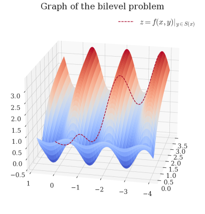
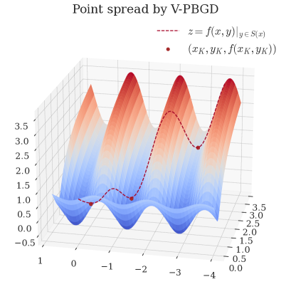
(a) Left figure: the graph of $z\!=\!f(x,y)$ and $z\!=\!f(x,y)|_{y\in\mathcal{S}(x)}$; right figure: the last iterates generated by $1000$ runs of V-PBGD with random initial points.

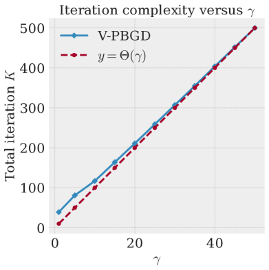
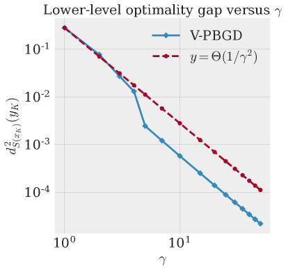
(b) Test of V-PBGD with different constant $\gamma$. The figure is generated by running V-PBGD (Algorithm 2) for $K$ steps such that $\|G_{\gamma}(x_{K},y_{K})\|^{2}\leq 10^{-4}$.

Figure 2: Test of V-PBGD in the bilevel problem (6.1).

6.2 Data hyper-cleaning

In this section, we test PBGD in the data hyper-cleaning task (Franceschi et al., 2017; Shaban et al., 2019). In this task, one is given a set of polluted training data, along with a set of clean validation and test data. The goal is to train a data cleaner that assigns smaller weights to the polluted data to improve the generalization in unseen clean data.

Method	Linear model		2-layer MLP
	Test accuracy	F1 score	Test accuracy	F1 score
RHG	$87.64\pm 0.19$	$89.71\pm 0.25$	$87.50\pm 0.23$	$89.41\pm 0.21$
T-RHG	$87.63\pm 0.19$	$89.04\pm 0.24$	$87.48\pm 0.22$	$89.20\pm 0.21$
BOME	$87.09\pm 0.14$	$89.83\pm 0.18$	$87.42\pm 0.16$	$89.26\pm 0.17$
G-PBGD	$90.09\pm 0.12$	$90.82\pm 0.19$	$92.17\pm 0.09$	$90.73\pm 0.27$
IAPTT-GM	$\textbf{90.44}\pm 0.14$	$\textbf{91.89}\pm 0.15$	$91.72\pm 0.11$	$91.82\pm 0.19$
V-PBGD	$\textbf{90.48}\pm 0.13$	$\textbf{91.99}\pm 0.14$	$\textbf{94.58}\pm 0.08$	$\textbf{93.16}\pm 0.15$

Table 3: Comparison of solution quality. The results are averaged over $20$ runs and $\pm$ is followed by an estimated margin of error under $95\%$ confidence. F1 score measures the quality of the data cleaner (Franceschi et al., 2017).

	RHG	T-RHG	BOME	G-PBGD	IAPTT-GM	V-PBGD
GPU memory (MB) linear	1369	1367	1149	1149	$1237$	$1149$
GPU memory (MB) MLP	7997	7757	1201	1235	2613	$1199$
Runtime (sec.) linear	73.21	32.28	5.92	7.72	693.65	9.12
Runtime (sec.) MLP	94.78	54.96	39.78	185.08	1310.63	207.53

Table 4: Comparison of GPU memory usage and the runtime to reach the highest test accuracy averaged over 20 runs.

We evaluate the performance of our algorithm in terms of speed, memory usage and solution quality in comparison with several competitive baseline algorithms including the IAPTT-GM (Liu et al., 2021c), BOME (Ye et al., 2022), RHG (Franceschi et al., 2017) and T-RHG (Shaban et al., 2019). In addition to V-PBGD, we also test G-PBGD which is a special case of PBGD with the lower-level gradient norm penalty $p(x,y)=\|\nabla_{y}g(x,y)\|^{2}$. The method proposed by (Mehra and Hamm, 2021) can be viewed as G-PBGD. Adopting the settings in (Franceschi et al., 2017; Liu et al., 2021c; Shaban et al., 2019), we randomly split the MNIST data-set into a training data-set of size $5000$, a validation set of size $5000$ and a test set of size $10000$; and pollute $50\%$ of the training data with uniformly drawn labels. Then we run the algorithms with a linear model and an MLP network.

We report the solution quality in Table 3. It can be observed that both PBGD algorithms achieve competitive performance, and V-PBGD achieves the best performance among the baselines. We also evaluate PBGD in terms of convergence speed and memory usage, which is reported in Table 4. It can be observed that PBGD does not have a steep increase in memory consumption or runtime as compared to the ITD baselines, indicating PBGD is potentially more scalable.

7 Conclusions

In this work, we study the bilevel optimization problem through the lens of the penalty method. We prove that the solutions of the penalized problem approximately solve the original bilevel problem under certain generic conditions verifiable with commonly made assumptions. To solve the penalized problem, we propose the penalty-based bilevel GD method and establish its finite-time convergence under unconstrained and constrained lower-level problems. Experiments verify the effectiveness of the proposed algorithm.

Appendix A Proof in Section 2

For ease of reading, we restate $\mathcal{BP}$ and $\mathcal{BP}_{\gamma p}$ below.

$$\mathcal{BP}:~{}~{}\min_{x,y}f(x,y)\,\,\,{\rm s.t.}\,\,x\in\mathcal{C},~{}y\in\mathcal{S}(x)\coloneqq\arg\min_{y\in\mathcal{U}(x)}g(x,y),$$

and

$$\mathcal{BP}_{\gamma p}:\min_{x,y}f(x,y)+\gamma p(x,y),~{}~{}~{}{\rm s.t.}~{}~{}~{}x\in\mathcal{C},~{}y\in\mathcal{U}(x).$$

A.1 Proof of Theorem 1

Theorem  1.

Assume $p(x,y)$ is an $\rho$-squared-distance-bound function and $f(x,\cdot)$ is $L$-Lipschitz continuous on $\mathcal{U}(x)$ for any $x\in\mathcal{C}$. Given any $\epsilon_{1}>0$, any global solution of $\mathcal{BP}$ is an $\epsilon_{1}$-global-minimum point of $\mathcal{BP}_{\gamma p}$ with any $\gamma\geq\gamma^{*}=\frac{L^{2}\rho}{4}\epsilon_{1}^{-1}$. Conversely, given $\epsilon_{2}\geq 0$, let $(x_{\gamma},y_{\gamma})$ achieves $\epsilon_{2}$-global-minimum of $\mathcal{BP}_{\gamma p}$ with $\gamma>\gamma^{*}$. Then $(x_{\gamma},y_{\gamma})$ achieves $\epsilon_{2}$-global-minimum of the following approximate problem of $\mathcal{BP}$ with some $0\leq\epsilon_{\gamma}\leq(\epsilon_{1}\!+\!\epsilon_{2})/(\gamma\!-\!\gamma^{*})$; given by

$$\min_{x,y}f(x,y)~{}~{}~{}{\rm s.t.}~{}~{}~{} x\in\mathcal{C},~{}y\in\mathcal{U}(x),$$

$$p(x,y)\leq\epsilon_{\gamma}.$$ (A.1)

Proof.

Given any $x\in\mathcal{C}$ and $y\in\mathcal{U}(x)$, since $\mathcal{S}(x)$ is closed and non-empty, we can find $y_{x}\in\arg\min_{y^{\prime}\in\mathcal{S}(x)}\|y^{\prime}-y\|$. By Lipschitz continuity assumption on $f(x,\cdot)$, given any $x\in\mathcal{C}$, it holds for any $y\in\mathcal{U}(x)$ that

$$f(x,y)-f(x,y_{x}) \geq-Ld_{\mathcal{S}(x)}(y)\quad\text{by }d_{\mathcal{S}(x)}(y)=\|y_{x}-y\|.$$

Then it follows that

$$f(x,y)+\gamma^{*}p(x,y)-f(x,y_{x}) \geq-Ld_{\mathcal{S}(x)}(y)+\gamma^{*}p(x,y)$$

$$\geq-Ld_{\mathcal{S}(x)}(y)+\frac{\gamma^{*}}{\rho}d_{\mathcal{S}(x)}^{2}(y)$$

$$\geq\min_{z\in\mathbb{R}_{\geq 0}}-Lz+\frac{\gamma^{*}}{\rho}z^{2}=-\epsilon_{1}\quad\text{with }\gamma^{*}=\frac{L^{2}\rho}{4}\epsilon_{1}^{-1}.$$ (A.2)

Since $y_{x}\in\mathcal{S}(x)$ (thus $y_{x}\in\mathcal{U}(x)$) and $x\in\mathcal{C}$, $(x,y_{x})$ is feasible for $\mathcal{BP}$. Let $f^{*}$ be the optimal objective value for $\mathcal{BP}$, we know $f(x,y_{x})\geq f^{*}$. This along with (A.1) indicates

$$f(x,y)+\gamma^{*}p(x,y)-f^{*}\geq-\epsilon_{1},~{}~{}\forall x\in\mathcal{C},~{}y\in\mathcal{U}(x).$$ (A.3)

Let $(x^{*},y^{*})$ be a global solution of $\mathcal{BP}$ so that $f(x^{*},y^{*})=f^{*}$. Since $y^{*}\in\mathcal{S}(x^{*})$, $p(x^{*},y^{*})=0$ . By (A.3), we have

$$f(x^{*},y^{*})+\gamma^{*}p(x^{*},y^{*})\leq f(x,y)+\gamma^{*}p(x,y)+\epsilon_{1},~{}~{}\forall x\in\mathcal{C},~{}\forall y\in\mathcal{U}(x).$$ (A.4)

Inequality (A.4) along with the fact that the global solution of $\mathcal{BP}$ is feasible for $\mathcal{BP}_{\gamma p}$ prove that the global solution of $\mathcal{BP}$ achieves $\epsilon_{1}$-global-minimum for $\mathcal{BP}_{\gamma p}$.

Now for the converse part. Since $(x_{\gamma},y_{\gamma})$ achieves $\epsilon_{2}$-global-minimum, it holds for any $x,y$ feasible for $\mathcal{BP}_{\gamma p}$ that

$$f(x_{\gamma},y_{\gamma})+\gamma p(x_{\gamma},y_{\gamma})-\epsilon_{1}\leq f(x,y)+\gamma p(x,y)-\epsilon_{1}+\epsilon_{2}.$$ (A.5)

In (A.5), choosing $(x,y)=(x^{*},y^{*})$ which is a global solution of $\mathcal{BP}$ yields

$$f(x_{\gamma},y_{\gamma})+\gamma p(x_{\gamma},y_{\gamma})-\epsilon_{1} \leq f(x^{*},y^{*})-\epsilon_{1}+\epsilon_{2}\quad\text{since }p(x^{*},y^{*})=0$$

$$\leq f(x_{\gamma},y_{\gamma})+\gamma^{*}p(x_{\gamma},y_{\gamma})+\epsilon_{2}\quad\text{by \eqref{eq:global calmness 1}.}$$

Then we have

$$(\gamma-\gamma^{*})p(x_{\gamma},y_{\gamma})\leq\epsilon_{1}+\epsilon_{2}\Rightarrow p(x_{\gamma},y_{\gamma})\leq(\epsilon_{1}+\epsilon_{2})/(\gamma-\gamma^{*}).$$

Define $\epsilon_{\gamma}=p(x_{\gamma},y_{\gamma})$, then $\epsilon_{\gamma}\leq(\epsilon_{1}+\epsilon_{2})/(\gamma-\gamma^{*})$. By (A.5), it holds for any $(x,y)$ feasible for problem (Theorem  1) that

$$f(x_{\gamma},y_{\gamma})+\gamma p(x_{\gamma},y_{\gamma})\leq f(x,y)+\gamma p(x,y)+\epsilon_{2}\Rightarrow f(x_{\gamma},y_{\gamma})-f(x,y)\leq\gamma(p(x,y)-\epsilon_{\gamma})+\epsilon_{2}\leq\epsilon_{2},$$

where the last inequality follows from the feasibility of $(x,y)$. This along with the fact that $(x_{\gamma},y_{\gamma})$ is feasible for problem (Theorem  1) prove that $(x_{\gamma},y_{\gamma})$ achieves $\epsilon_{2}$-global-minimum of problem (Theorem  1). ∎

A.2 Proof of Theorem 2

In this section, we give the proof of a stronger version of Theorem 2 in the sense of weaker assumptions.

We first define a new class of functions as follows.

Definition 3 (Restricted $\alpha$-sublinearity).

Let $\mathcal{X}\subseteq\mathbb{R}^{d}$. We say a function $\ell:\mathcal{X}\mapsto\mathbb{R}$ is restricted $\alpha$-sublinear on $x\in\mathcal{X}$ if there exists $\alpha\in[0,1]$ and $x^{*}\in\mathcal{X}$ which is the projection of $x$ onto the minimum point set of $\ell$ such that the following inequality holds.

$$\ell\big{(}(1-\alpha)x+\alpha x^{*}\big{)}\leq(1-\alpha)\ell(x)+\alpha\ell(x^{*}).$$

Suppose $\ell$ is a continuous convex or more generally a star-convex function [Nesterov and Polyak, 2006, Definition 1] defined on a closed convex set $\mathcal{X}$ and $\ell$ has a non-empty minimum point set, then $\ell$ is restricted $\alpha$-sublinear for any $\alpha\in[0,1]$ on every $x\in\mathcal{X}$.

Now we are ready to give the stronger version of Theorem 2.

Theorem 6 (Stronger version of Theorem 2).

Assume $p(x,\cdot)$ is continuous given any $x\in\mathcal{C}$ and $p(x,y)$ is $\rho$-squared-distance-bound function. Given $\gamma>0$, let $(x_{\gamma},y_{\gamma})$ be a local solution of $\mathcal{BP}_{\gamma p}$ on $\mathcal{N}((x_{\gamma},y_{\gamma}),r)$. Assume $f(x_{\gamma},\cdot)$ is $L$-Lipschitz-continuous on $\mathcal{N}(y_{\gamma},r)$.

Assume either one of the following is true:

1. There exists $\bar{y}\in\mathcal{N}(y_{\gamma},r)$ such that $\bar{y}\in\mathcal{U}(x_{\gamma})$ and $p(x_{\gamma},\bar{y})\leq\epsilon$ for some $\epsilon\geq 0$. Define $\bar{\epsilon}_{\gamma}=\frac{L^{2}\rho}{\gamma^{2}}\!+\!2\epsilon$.

2. The set $\mathcal{U}(x_{\gamma})$ is convex and $p(x_{\gamma},\cdot)$ is restricted $\alpha$-sublinear on $y_{\gamma}$ with some $\alpha\in(0,\min\{\frac{r}{d_{\mathcal{S}(x_{\gamma})}(y_{\gamma})},1\}]$. Define $\bar{\epsilon}_{\gamma}=\frac{L^{2}\rho}{\gamma^{2}}$.

Then $(x_{\gamma},y_{\gamma})$ is a local solution of the following approximate problem of $\mathcal{BP}$ with $0\leq\epsilon_{\gamma}\leq\bar{\epsilon}_{\gamma}$.

$$\min_{x,y}f(x,y)~{}~{}~{}{\rm s.t.}~{}~{}~{} x\in\mathcal{C},~{}y\in\mathcal{U}(x)$$ (A.6)

$$p(x,y)\leq\epsilon_{\gamma}.$$

The above theorem is stronger than Theorem 2 in the sense that the condition (ii) in above theorem is weaker than (ii) in Theorem 2 since the continuity and convexity of $p(x_{\gamma},\cdot)$ implies the restricted $\alpha$-sublinearity of $p(x_{\gamma},\cdot)$ on $y_{\gamma}$ with any $\alpha\in[0,1]$.

Proof of Theorem 6.

We will prove the theorem for two cases separately.

(i). Assume (i) is true. For $\delta\geq 0$, define

$$\mathcal{S}_{\delta}(x)\coloneqq\{y\in\mathcal{U}(x):p(x,y)\leq\delta\},~{}x\in\mathcal{C}.$$

Since $p(x,y)=0$ if and only if (iff) $y\in\mathcal{S}(x)=\arg\min_{y\in\mathcal{U}(x)}g(x,y)$, it follows that $\mathcal{S}(x)=\{y\in\mathcal{U}(x):p(x,y)=0\}$. Then $\mathcal{S}_{\delta}(x)\supseteq\mathcal{S}(x)$, and thus $\mathcal{S}_{\delta}(x)\neq\emptyset$. Moreover, $\mathcal{S}_{\delta}(x)$ is closed by continuity of $p(x,\cdot)$ and closeness of $\mathcal{U}(x)$ for $x\in\mathcal{C}$.

Since $(x_{\gamma},y_{\gamma})$ is a local solution of $\mathcal{BP}_{\gamma p}$ on $\mathcal{N}((x_{\gamma},y_{\gamma}),r)$, it holds for any $(x,y)\in\mathcal{N}((x_{\gamma},y_{\gamma}),r)$ that is feasible for $\mathcal{BP}_{\gamma p}$ that

$$f(x_{\gamma},y_{\gamma})+\gamma p(x_{\gamma},y_{\gamma})\leq f(x,y)+\gamma p(x,y).$$ (A.7)

Since $\mathcal{S}_{\epsilon}(x_{\gamma})$ is closed and non-empty, we can find $y_{x}\in\arg\min_{y^{\prime}\in\mathcal{S}_{\epsilon}(x_{\gamma})}\|y^{\prime}-y_{\gamma}\|$. Since $\bar{y}\in\mathcal{N}(y_{\gamma},r)\cap\mathcal{S}_{\epsilon}(x_{\gamma})$, we have $\|{y_{x}-y_{\gamma}}\|\leq\|{\bar{y}-y_{\gamma}}\|\leq r$. This indicates $y_{x}\in\mathcal{N}(y_{\gamma},r)$ and $(x_{\gamma},y_{x})\in\mathcal{N}((x_{\gamma},y_{\gamma}),r)$. Moreover, since $y_{x}\in\mathcal{U}(x_{\gamma})$, $(x_{\gamma},y_{x})$ is feasible for $\mathcal{BP}_{\gamma p}$. This allows to choose $(x,y)=(x_{\gamma},y_{x})$ in (A.7), leading to

$$f(x_{\gamma},y_{\gamma})+\gamma p(x_{\gamma},y_{\gamma})\leq f(x_{\gamma},y_{x})+\gamma\epsilon\quad\text{since }y_{x}\in\mathcal{S}_{\epsilon}(x_{\gamma}).$$

By Lipschitz continuity of $f(x_{\gamma},\cdot)$ on $\mathcal{N}(y_{\gamma},r)$, we further have

$$\gamma p(x_{\gamma},y_{\gamma})-L\|y_{x}-y_{\gamma}\|-\gamma\epsilon \leq 0.$$ (A.8)

Since $\mathcal{S}_{\epsilon}(x_{\gamma})\supseteq\mathcal{S}(x_{\gamma})$, we have $\|y_{x}-y_{\gamma}\|=d_{\mathcal{S}_{\epsilon}(x_{\gamma})}(y_{\gamma})\leq d_{\mathcal{S}(x_{\gamma})}(y_{\gamma})\leq\sqrt{\rho p(x_{\gamma},y_{\gamma})}$. Plugging this into (A.8) yields

$$\gamma p(x_{\gamma},y_{\gamma})-L\sqrt{\rho p(x_{\gamma},y_{\gamma})}-\gamma\epsilon \leq 0$$

which implies $p(x_{\gamma},y_{\gamma})\leq\bar{\epsilon}_{\gamma}=\frac{L^{2}\rho}{\gamma^{2}}+2\epsilon$. Let $\epsilon_{\gamma}=p(x_{\gamma},y_{\gamma})$, then $\epsilon_{\gamma}\leq\bar{\epsilon}_{\gamma}$ and $(x_{\gamma},y_{\gamma})$ is feasible for problem (A.6). By (A.7), it holds for any $(x,y)\in\mathcal{N}((x_{\gamma},y_{\gamma}),r)$ that are feasible for problem (A.6) that

$$f(x_{\gamma},y_{\gamma})-f(x,y)\leq\gamma(p(x,y)-\epsilon_{\gamma})\leq 0.$$

This and the fact that $(x_{\gamma},y_{\gamma})$ is feasible for (A.6) imply $(x_{\gamma},y_{\gamma})$ is a local solution of (A.6).

(ii). Assume (ii) is true. Since $\mathcal{S}(x_{\gamma})$ is closed and non-empty, we can find $y_{x}$ such that $y_{x}\in\arg\min_{y\in\mathcal{S}(x_{\gamma})}\|y-y_{\gamma}\|$. Let $\bar{y}=(1-\alpha)y_{\gamma}+\alpha y_{x}$. Since $0<\alpha\leq\min\{r/\|y_{\gamma}-y_{x}\|,1\}$, we know $\bar{y}\in\mathcal{N}(y_{\gamma},r)$ and $(x_{\gamma},\bar{y})\in\mathcal{N}((x_{\gamma},y_{\gamma}),r)$. Moreover, since $\mathcal{U}(x_{\gamma})$ is convex, we have $\bar{y}\in\mathcal{U}(x_{\gamma})$ and $(x_{\gamma},\bar{y})$ is feasible for $\mathcal{BP}_{\gamma p}$.

Since $(x_{\gamma},y_{\gamma})$ is a local solution of $\mathcal{BP}_{\gamma p}$ on $\mathcal{N}((x_{\gamma},y_{\gamma}),r)$, we have

$$f(x_{\gamma},y_{\gamma})+\gamma p(x_{\gamma},y_{\gamma}) \leq f(x_{\gamma},\bar{y})+\gamma p(x_{\gamma},\bar{y}).$$ (A.9)

Since $p(x_{\gamma},y)\geq 0$ and $p(x_{\gamma},y)=0$ iff $d_{\mathcal{S}(x_{\gamma})}(y)=0$, we know the minimum point set of $p(x_{\gamma},\cdot)$ is $\mathcal{S}(x_{\gamma})$. Then by the restricted $\alpha$-sublinearity of $p(x_{\gamma},\cdot)$ on $y_{\gamma}$, we have

$$p(x_{\gamma},\bar{y})\leq\alpha p(x_{\gamma},y_{x})+(1-\alpha)p(x_{\gamma},y_{\gamma})=(1-\alpha)p(x_{\gamma},y_{\gamma}).$$

Substituting the above inequality into (A.9) yields

$$f(x_{\gamma},y_{\gamma})+\gamma p(x_{\gamma},y_{\gamma}) \leq f(x_{\gamma},\bar{y})+\gamma(1-\alpha)p(x_{\gamma},y_{\gamma}).$$

Re-arranging the above inequality and using the Lipschitz continuity of $f(x_{\gamma},\cdot)$ on $\mathcal{N}(y_{\gamma},r)$ yield

$$\gamma\alpha p(x_{\gamma},y_{\gamma})\leq L\alpha d_{\mathcal{S}(x_{\gamma})}(y_{\gamma})\Rightarrow\gamma\alpha p(x_{\gamma},y_{\gamma})\leq L\alpha\sqrt{\rho p(x_{\gamma},y_{\gamma})}$$ (A.10)

which implies $p(x_{\gamma},y_{\gamma})\leq\bar{\epsilon}_{\gamma}=\frac{L^{2}\rho}{\gamma^{2}}$. Let $\epsilon_{\gamma}=p(x_{\gamma},y_{\gamma})$, then $\epsilon_{\gamma}\leq\bar{\epsilon}_{\gamma}$ and $(x_{\gamma},y_{\gamma})$ is feasible for problem (A.6). Since $(x_{\gamma},y_{\gamma})$ is a local solution of $\mathcal{BP}_{\gamma p}$ on $\mathcal{N}((x_{\gamma},y_{\gamma}),r)$, it holds for any $(x,y)\in\mathcal{N}((x_{\gamma},y_{\gamma}),r)$ that is feasible for $\mathcal{BP}_{\gamma p}$ that

$$f(x_{\gamma},y_{\gamma})+\gamma p(x_{\gamma},y_{\gamma})\leq f(x,y)+\gamma p(x,y).$$

Following from the above inequality, it holds for any $(x,y)\in\mathcal{N}((x_{\gamma},y_{\gamma}),r)$ that are feasible for problem (A.6) that

$$f(x_{\gamma},y_{\gamma})-f(x,y)\leq\gamma(p(x,y)-\epsilon_{\gamma})\leq 0.$$

This and the fact that $(x_{\gamma},y_{\gamma})$ is feasible for (A.6) imply $(x_{\gamma},y_{\gamma})$ is a local solution of (A.6). ∎

Appendix B Proof in Section 3

B.1 Proof of Lemma 1

(i). Assume (i) in this lemma holds. By the definition of $v(x)$, it is clear that $g(x,y)-v(x)\geq 0$ for any $x\in\mathcal{C}$ and $y\in\mathbb{R}^{d_{y}}$. Since $\mathcal{S}(x)$ is closed, $y\in\mathcal{S}(x)$ iff $d_{\mathcal{S}(x)}(y)=0$. Then by the definition of $\mathcal{S}(x)$, it holds for any $x\in\mathcal{C}$ and $y\in\mathbb{R}^{d_{y}}$ that

$$g(x,y)-v(x)=0~{}\text{iff}~{}y\in\mathcal{S}(x)\Rightarrow g(x,y)-v(x)=0~{}\text{iff}~{}d_{S(x)}(y)=0.$$

It then suffices to check whether $g(x,y)-v(x)$ is an upper-bound of $d_{S(x)}(y)$. By $\frac{1}{\mu}$-PL condition of $g(x,\cdot)$ and [Karimi et al., 2016, Theorem 2], $g(x,\cdot)$ satisfies the $\frac{1}{\mu}$-quadratic-growth condition, and thus for any $x\in\mathcal{C}$ and $y\in\mathbb{R}^{d_{y}}$, it holds that

$$g(x,y)-v(x)\geq\frac{1}{\mu}d_{S(x)}^{2}(y).$$ (B.1)

This completes the proof.

(ii). Assume (ii) in this lemma holds. We consider when $g(x,\cdot)$ satisfies PL condition given any $x\in\mathcal{C}$. By the PL inequality, it is clear that $\|\nabla_{y}g(x,y)\|^{2}=0$ is equivalent to $g(x,y)=\min_{y\in\mathbb{R}^{d_{y}}}g(x,y)$ given any $x\in\mathcal{C}$, thus $\|\nabla_{y}g(x,y)\|^{2}=0$ iff $d_{\mathcal{S}(x)}(y)=0$ for any $x\in\mathcal{C}$.

By $\frac{1}{\sqrt{\mu}}$-PL condition of $g(x,\cdot)$, we have $\|\nabla_{y}g(x,y)\|^{2}\geq\frac{1}{\sqrt{\mu}}(g(x,y)-v(x))$. By (B.1), we have $g(x,y)-v(x)\geq\frac{1}{\sqrt{\mu}}d_{S(x)}^{2}(y)$. Thus it holds that

$$\|\nabla_{y}g(x,y)\|^{2}\geq\frac{1}{\mu}d_{S(x)}^{2}(y),$$

which completes the proof.

B.2 Proof of Proposition 2

We prove the proposition from the two conditions separately.

(a) Since $(x_{\gamma},y_{\gamma})$ is a local solution of $\mathcal{UP}_{\gamma p}$, $y_{\gamma}$ is a local solution of $\mathcal{UP}_{\gamma p}$ with $x=x_{\gamma}$. By the first-order stationary condition, it holds that

$$\nabla_{y}f(x_{\gamma},y_{\gamma})+\gamma\nabla_{y}g(x_{\gamma},y_{\gamma})=0\Rightarrow\|\nabla_{y}g(x_{\gamma},y_{\gamma})\|\leq L/\gamma.$$

Since $g(x_{\gamma},\cdot)$ satisfies $1/\mu$-PL inequality, it holds that

$$\|\nabla_{y}g(x_{\gamma},y_{\gamma})\|^{2}\geq\frac{1}{\mu}p(x_{\gamma},y_{\gamma}).$$

The above two inequalities imply $p(x_{\gamma},y_{\gamma})\leq\frac{L^{2}\mu}{\gamma^{2}}$. Further notice that $\mathcal{UP}$ and $\mathcal{UP}_{\gamma p}$ are respectively special cases of $\mathcal{BP}$ and $\mathcal{BP}_{\gamma p}$ with $\mathcal{U}(x)=\mathbb{R}^{d_{y}}$; and $p(x,y)$ is a squared distance bound by Lemma 1, then the result directly follows from Theorem 2 where condition $(i)$ is met with $\bar{y}=y_{\gamma}$, $\rho=\mu$ and $\epsilon=\frac{L^{2}\mu}{\gamma^{2}}$ with $\gamma\geq L\sqrt{3\mu\delta^{-1}}$.

(b) Suppose $y_{\gamma}\notin\mathcal{S}(x_{\gamma})$. Since $(x_{\gamma},y_{\gamma})$ is a local solution of $\mathcal{UP}_{\gamma p}$, $y_{\gamma}$ is a local solution of $\mathcal{UP}_{\gamma p}$ with $x=x_{\gamma}$. By the first-order stationary condition, it holds that

$$\nabla_{y}f(x_{\gamma},y_{\gamma})+2\gamma\nabla_{yy}g(x_{\gamma},y_{\gamma})\nabla_{y}g(x_{\gamma},y_{\gamma})=0\Rightarrow\|\nabla_{yy}g(x_{\gamma},y_{\gamma})\nabla_{y}g(x_{\gamma},y_{\gamma})\|\leq L/2\gamma$$

which along with the assumption that the singular values of $\nabla_{yy}g(x,y)$ on $\{x\in\mathcal{C},y\in\mathcal{U}(x):y\notin\mathcal{S}(x)\}$ are lower bounded by $\sigma>0$ gives

$$p(x_{\gamma},y_{\gamma})=\|\nabla_{y}g(x_{\gamma},y_{\gamma})\|^{2}\leq\frac{\|\nabla_{yy}g(x_{\gamma},y_{\gamma})\nabla_{y}g(x_{\gamma},y_{\gamma})\|^{2}}{\sigma^{2}}\leq L^{2}/(4\gamma^{2}\sigma^{2}).$$ (B.2)

When $y_{\gamma}\in\mathcal{S}(x_{\gamma})$, we know $p(x_{\gamma},y_{\gamma})=0$ and thus (B.2) still holds. Further notice that $\mathcal{UP}$ and $\mathcal{UP}_{\gamma p}$ are special cases of $\mathcal{BP}$ and $\mathcal{BP}_{\gamma p}$ with $\mathcal{U}(x)=\mathbb{R}^{d_{y}}$; and $p(x,y)$ is a squared distance bound by Lemma 1, then the result directly follows from Theorem 2 where condition $(i)$ is met with $\bar{y}=y_{\gamma}$, $\rho=\mu$ and $\epsilon=L^{2}/(4\gamma^{2}\sigma^{2})$ with $\gamma\geq\max\{L\sqrt{2\mu\delta^{-1}},L\sqrt{\delta^{-1}}/\sigma\}$.

B.3 Proof of Theorem 3

We first provide the convergence theorem on the sequence $\{\omega_{t}^{(k)}\}$ given the outer iteration $k$.

Theorem 7.

Assume there exist $L_{g}>0$ and $\mu>0$ such that $g(x,\cdot)$ is $L_{g}$-Lipschitz-smooth and $\frac{1}{\mu}$-PL given any $x\in\mathcal{C}$. Choose $\beta\in(0,\frac{1}{L_{g}}]$. Given any $x_{k}\in C$, $\omega_{1}^{(k)}\in\mathbb{R}^{d_{y}}$, running $T_{k}$ steps of inner GD updates (3.4a) gives $\hat{y}_{k}$ satisfying

$$d_{S(x_{k})}^{2}(\hat{y}_{k})\leq\mu\big{(}1-\frac{\beta}{2\mu}\big{)}^{T_{k}}\big{(}g(x_{k},\omega_{1}^{(k)})-v(x_{k})\big{)}.$$ (B.3)

Proof of Theorem 7.

We omit all index $k$ since this proof holds given any $k$. By Lipschitz smoothness of $g(x,\cdot)$, it holds that

$$g(x,\omega_{t+1}) \leq g(x,\omega_{t})-\beta\|\nabla_{y}g(x,\omega_{t})\|^{2}+\frac{L_{g}\beta^{2}}{2}\|\nabla_{y}g(x,\omega_{t})\|^{2}$$

$$\leq g(x,\omega_{t})-\frac{\beta}{2}\|\nabla_{y}g(x,\omega_{t})\|^{2}\quad\text{since}~{}L_{g}\beta\leq 1.$$

By $\frac{1}{\mu}$-PL condition of $g(x,\cdot)$, we further have

$$g(x,\omega_{t+1})-v(x) \leq g(x,\omega_{t})-v(x)-\frac{\beta}{2\mu}\big{(}g(x,\omega_{t})-v(x)\big{)}$$

$$\leq\big{(}1-\frac{\beta}{2\mu}\big{)}\big{(}g(x,\omega_{t})-v(x)\big{)}.$$

Iteratively applying the above inequality for $t=1,\dots,T$ yields

$$g(x,\omega_{T+1})-v(x)\leq\big{(}1-\frac{\beta}{2\mu}\big{)}^{T}\big{(}g(x,\omega_{1})-v(x)\big{)}.$$ (B.4)

By [Karimi et al., 2016, Theorem 2], the $\frac{1}{\mu}$-PL condition of $g(x,\cdot)$ also implies the error bound of $g(x,\cdot)$, which leads to

$$g(x,\omega_{T+1})-v(x)\geq\frac{1}{\mu}d_{S(x)}^{2}(\omega_{T+1}),~{}x\in\mathcal{C}$$

which along with (B.4) proves the result in (B.3). ∎

Notice the term $g(x_{k},\omega_{1}^{(k)})-v(x_{k})$ in (B.3) depends on the drifting variable $x_{k}$. If $\omega_{1}^{(k)}$ is not carefully chosen, $g(x_{k},\omega_{1}^{(k)})-v(x_{k})$ can grow unbounded with $k$ and hence hinder the convergence. To prevent this, we choose $\omega_{1}^{(k)}=y_{k}$ in the analysis. Since $g(x,\cdot)$ is $\frac{1}{\mu}$-PL for any $x\in\mathcal{C}$, it holds that

$$g(x_{k},\omega_{1}^{(k)})-v(x_{k})\leq\frac{1}{\mu}\|\nabla_{y}g(x_{k},\omega_{1}^{(k)})\|^{2} =\frac{1}{\mu}\left\|{\frac{y_{k}-y_{k+1}-\alpha\nabla_{y}f(x_{k},y_{k})}{\alpha\gamma}}\right\|^{2}$$

$$\leq\frac{2}{\mu\gamma^{2}\alpha^{2}}\|y_{k+1}-y_{k}\|^{2}+\frac{2L^{2}}{\mu\gamma^{2}}$$ (B.5)

where we have used Young’s inequality and the condition that $f(x_{k},\cdot)$ is $L$-Lipschitz-continuous. Later we will show that the inexact gradient descent update (3.4b) decreases $\|(x_{k+1},y_{k+1})-(x_{k},y_{k})\|$ and therefore upper-bounds $g(x_{k},\omega_{1}^{(k)})-v(x_{k})$.

Next we give the proof of Theorem 3.

Proof of Theorem 3.

In this proof, we write $z=(x,y)$. Update (3.4b) can be written as

$$z_{k+1}=\operatorname{Proj}_{\mathcal{Z}}\big{(}z_{k}-\alpha\hat{\nabla}F_{\gamma}(z_{k};\hat{y}_{k})\big{)}$$

where $\hat{\nabla}F_{\gamma}(z_{k};\hat{y}_{k}\big{)}\coloneqq\nabla f(z_{k})+\gamma(\nabla g(z_{k})-\overline{\nabla}_{x}g(x_{k},\hat{y}_{k})\big{)}$.

By the assumptions made in this theorem and Lemma 2, $F_{\gamma}$ is $L_{\gamma}$-Lipschitz-smooth with $L_{\gamma}=L_{f}+\gamma(2L_{g}+L_{g}^{2}\mu)$. Then by Lipschitz-smoothness of $F_{\gamma}$, it holds that

$$F_{\gamma}(z_{k+1}) \leq F_{\gamma}(z_{k})+\langle{\nabla F_{\gamma}(z_{k})},\,{z_{k+1}-z_{k}}\rangle+\frac{L_{\gamma}}{2}\|z_{k+1}-z_{k}\|^{2}$$

$$\stackrel{{\scriptstyle\alpha\leq\frac{1}{L_{\gamma}}}}{{\leq}}F_{\gamma}(z_{k})+\langle{\hat{\nabla}F_{\gamma}(z_{k};\hat{y}_{k})},\,{z_{k+1}-z_{k}}\rangle+\frac{1}{2\alpha}\|z_{k+1}-z_{k}\|^{2}+\langle{\nabla F_{\gamma}(z_{k})-\hat{\nabla}F_{\gamma}(z_{k};\hat{y}_{k})},\,{z_{k+1}-z_{k}}\rangle.$$ (B.6)

Consider the second term in the RHS of (B.3). By Lemma 4, $z_{k+1}$ can be written as

$$z_{k+1}=\arg\min_{z\in\mathcal{Z}}\langle{\hat{\nabla}F_{\gamma}(z_{k};\hat{y}_{k})},\,{z}\rangle+\frac{1}{2\alpha}\|z-z_{k}\|^{2}.$$

By the first-order optimality condition of the above problem, it holds that

$$\langle{\hat{\nabla}F_{\gamma}(z_{k};\hat{y}_{k})+\frac{1}{\alpha}(z_{k+1}-z_{k})},\,{z_{k+1}-z}\rangle\leq 0,~{}\forall z\in\mathcal{Z}.$$

Since $z_{k}\in\mathcal{Z}$, we can choose $z=z_{k}$ in the above inequality and obtain

$$\langle{\hat{\nabla}F_{\gamma}(z_{k};\hat{y}_{k})},\,{z_{k+1}-z_{k}}\rangle\leq-\frac{1}{\alpha}\|z_{k+1}-z_{k}\|^{2}.$$ (B.7)

Consider the last term in the RHS of (B.3). By Young’s inequality, we first have

$$\langle{\nabla F_{\gamma}(z_{k})-\hat{\nabla}F_{\gamma}(z_{k};\hat{y}_{k})},\,{z_{k+1}-z_{k}}\rangle\leq\alpha\|{\nabla F_{\gamma}(z_{k})-\hat{\nabla}F_{\gamma}(z_{k};\hat{y}_{k})}\|^{2}+\frac{1}{4\alpha}\|{z_{k+1}-z_{k}}\|^{2}$$ (B.8)

where the first term in the above inequality can be bounded as

$$\|{\nabla F_{\gamma}(z_{k})-\hat{\nabla}F_{\gamma}(z_{k};\hat{y}_{k})}\|^{2} =\gamma^{2}\|{\nabla v(x_{k})-\overline{\nabla}_{x}g(x_{k},\hat{y}_{k})}\|^{2}$$

$$=\gamma^{2}\|{\nabla g(x_{k},y^{*})|_{y^{*}\in\mathcal{S}(x_{k})}-\overline{\nabla}_{x}g(x_{k},\hat{y}_{k})}\|^{2}\quad\text{by Lemma \ref{lem:grad vx}},$$

$$\leq\gamma^{2}L_{g}^{2}d^{2}_{\mathcal{S}(x_{k})}(\hat{y}_{k})\quad\text{by choosing $y^{*}\in\arg\min_{y^{\prime}\in\mathcal{S}(x_{k})}\|{y^{\prime}-\hat{y}_{k}}\|$},$$

$$\leq\gamma^{2}L_{g}^{2}\mu\big{(}1-\frac{\beta}{2\mu}\big{)}^{T_{k}}\big{(}g(x_{k},\omega_{1}^{(k)})-v(x_{k})\big{)}\quad\text{by Theorem \ref{the:nonconvex omega convergence}},$$

$$\leq\big{(}1-\frac{\beta}{2\mu}\big{)}^{T_{k}}\big{(}\frac{2L_{g}^{2}}{\alpha^{2}}\|{z_{k+1}-z_{k}}\|^{2}+2L^{2}L_{g}^{2}\big{)}\quad\text{by \eqref{eq:omega1 upper-bound}},$$

$$\leq\frac{1}{8\alpha^{2}}\|{z_{k+1}-z_{k}}\|^{2}+\frac{L^{2}L_{g}^{2}}{2\alpha^{2}k^{2}}$$ (B.9)

where the last inequality requires $T_{k}\geq\max\{-\log_{c_{\beta}}(16L_{g}^{2}),-2\log_{c_{\beta}}(2\alpha k)\}~{}\text{with}~{}c_{\beta}=1-\frac{\beta}{2\mu}$.

Plugging the inequality (B.3) into (B.8) yields

$$\langle{\nabla F_{\gamma}(z_{k})-\hat{\nabla}F_{\gamma}(z_{k};\hat{y}_{k})},\,{z_{k+1}-z_{k}}\rangle\leq\frac{3}{8\alpha}\|{z_{k+1}-z_{k}}\|^{2}+\frac{L^{2}L_{g}^{2}}{2\alpha k^{2}}.$$ (B.10)

Substituting (B.10) and (B.7) into (B.3) and rearranging the resulting inequality yield

$$\frac{1}{8\alpha}\|z_{k+1}-z_{k}\|^{2}\leq F_{\gamma}(z_{k})-F_{\gamma}(z_{k+1})+\frac{L^{2}L_{g}^{2}}{2\alpha k^{2}}.$$ (B.11)

With $\bar{z}_{k+1}$ defined in (3.5), we have

$$\|{\bar{z}_{k+1}-z_{k}}\|^{2} \leq 2\|{\bar{z}_{k+1}-z_{k+1}}\|^{2}+2\|z_{k+1}-z_{k}\|^{2}$$

$$\leq 2\alpha^{2}\|{\nabla F_{\gamma}(z_{k})-\hat{\nabla}F_{\gamma}(z_{k};\hat{y}_{k})}\|^{2}\!+\!2\|z_{k+1}\!-\!z_{k}\|^{2}$$

$$\leq\frac{9}{4}\|z_{k+1}-z_{k}\|^{2}+\frac{L^{2}L_{g}^{2}}{k^{2}}$$ (B.12)

where the second inequality uses non-expansiveness of $\operatorname{Proj}_{\mathcal{Z}}$ and the last one follows from (B.3).

Together (B.11) and (B.3) imply

$$\|{\bar{z}_{k+1}-z_{k}}\|^{2}\leq 18\alpha\big{(}F_{\gamma}(z_{k})-F_{\gamma}(z_{k+1})\big{)}+\frac{10L^{2}L_{g}^{2}}{k^{2}}.$$

Since $f(z)\geq C_{f}$ for any $z\in\mathcal{Z}$ and $g(x,y)-v(x)\geq 0$, $F_{\gamma}(z)\geq C_{f}$ for any $z\in\mathcal{Z}$. Taking a telescope sum of the above inequality and using $G_{\gamma}(z_{k})=\frac{1}{\alpha}(z_{k}-\bar{z}_{k+1})$ yield

$$\sum_{k=1}^{K}\|G_{\gamma}(z_{k})\|^{2}\leq\frac{18\big{(}F_{\gamma}(z_{1})-C_{f}\big{)}}{\alpha}+\sum_{k=1}^{K}\frac{10L^{2}L_{g}^{2}}{k^{2}}$$

which along with the fact $\sum_{k=1}^{K}\frac{1}{k^{2}}\leq\int_{1}^{K}\frac{1}{x^{2}}dx=1-\frac{1}{K}$ implies

$$\sum_{k=1}^{K}\|G_{\gamma}(z_{k})\|^{2}\leq\frac{18\big{(}F_{\gamma}(z_{1})-C_{f}\big{)}}{\alpha}+10L^{2}L_{g}^{2}.$$ (B.13)

This proves (i) in Theorem 3.

Suppose $\lim_{k\rightarrow\infty}z_{k}=z^{*}$. Since $\nabla F_{\gamma}(z)$ is continuous, $G_{\gamma}(z)$ is continuous and thus $\lim_{k\rightarrow\infty}G_{\gamma}(z_{k})=G_{\gamma}(z^{*})$. By (B.13), $G_{\gamma}(z^{*})=0$, that is $z^{*}=\operatorname{Proj}_{\mathcal{Z}}\big{(}z^{*}-\alpha\nabla F_{\gamma}(z^{*})\big{)}$. This further implies

$$\langle{\nabla F_{\gamma}(z^{*})},\,{z^{*}-z}\rangle\leq 0,~{}\forall z\in\mathcal{Z}$$

which indicates $z^{*}$ is a stationary point of $\mathcal{UP}_{\gamma p}$. If $z^{*}$ is a local/global solution, it follows from Proposition 1 and 2 that the rest of the result holds. ∎

Lemma 4.

Let $\mathcal{Z}\subseteq\mathbb{R}^{d}$ be a closed convex set. Given any $z\in\mathcal{Z}$, $q\in\mathbb{R}^{d}$ and $\alpha>0$, it holds that

$$\operatorname{Proj}_{\mathcal{Z}}\big{(}z-\alpha q\big{)}=\arg\min_{z^{\prime}\in\mathcal{Z}}\langle{q},\,{z^{\prime}}\rangle+\frac{1}{2\alpha}\|z-z^{\prime}\|^{2}.$$

Proof.

Given $z\in\mathbb{R}^{d}$, define $z^{*}=\arg\min_{z^{\prime}\in\mathbb{R}^{d}}E(z^{\prime})$ where

$$E(z^{\prime})\coloneqq\langle{q},\,{z^{\prime}-z}\rangle+\frac{1}{2\alpha}\|z^{\prime}-z\|^{2}.$$ (B.14)

By the optimality condition, it follows $z^{*}=z-\alpha q$. For any $z^{\prime}\in\mathbb{R}^{d}$, it follows that

$$E(z^{\prime})-E(z^{*}) =\langle{q},\,{z^{\prime}-z}\rangle+\frac{1}{2\alpha}\|z^{\prime}-z\|^{2}-\langle{q},\,{-\alpha q}\rangle-\frac{\alpha}{2}\|{q}\|^{2}$$

$$=\frac{1}{2\alpha}\|z^{\prime}-z\|^{2}+\langle{q},\,{z^{\prime}-z}\rangle+\frac{\alpha}{2}\|q\|^{2}$$

$$=\frac{1}{2\alpha}\|z^{\prime}-(z-\alpha q)\|^{2}.$$ (B.15)

Then we have

$$\arg\min_{z^{\prime}\in\mathcal{Z}}\langle{q},\,{z^{\prime}}\rangle+\frac{1}{2\alpha}\|z-z^{\prime}\|^{2} =\arg\min_{z^{\prime}\in\mathcal{Z}}E(z^{\prime})$$

$$=\arg\min_{z^{\prime}\in\mathcal{Z}}\|z^{\prime}-(z-\alpha q)\|^{2}~{}~{}\text{ by \eqref{eq:idk279}}$$

$$=\operatorname{Proj}_{\mathcal{Z}}\big{(}z-\alpha q\big{)}.$$ (B.16)

This proves the result. ∎

B.4 Extension to the stochastic case

In Seciton 3, we have studied the deterministic V-PBGD algorithm. In this section, we extend the V-PBGD algorithm to the stochastic case.

With random variables $\xi,\psi$, we assume access to $\nabla g(x,y;\psi)$ and $\nabla f(x,y;\xi)$ which are respectively stochastic versions of $\nabla g(x,y)$ and $\nabla f(x,y)$. Following the idea of V-PBGD, given iteration $k$ and $x_{k}$, we first solve the lower-level problem with the stochastic gradient descent method:

$$\omega_{t+1}^{(k)}=\omega_{t}^{(k)}-\beta_{t}\nabla_{y}g(x_{k},\omega_{t}^{(k)};\psi_{t}^{(k)})~{}\text{for}~{}t=1,\dots,T_{k}$$ (B.17)

Then we choose the approximate lower-level solution $\hat{y}_{k}=\omega_{i}^{(k)}$ where $i$ is drawn from a step-size weighted distribution specified by $\mathbf{P}(i=t)=\beta_{t}/\sum_{t=1}^{T_{k}}\beta_{t},~{}t=1,...,T_{k}$. Given $\hat{y}_{k}$ and the batch size $M$, $(x_{k},y_{k})$ is updated with the approximate stochastic gradient of $F_{\gamma}(x_{k},y_{k})$ as follows:

$$(x_{k+1},y_{k+1})\!=\!\operatorname{Proj}_{\mathcal{Z}}\Big{(}(x_{k},y_{k})-\frac{\alpha_{k}}{M}\sum_{i=1}^{M}\big{(}\nabla f(x_{k},y_{k};\xi_{k}^{i})\!+\!\gamma(\nabla g(x_{k},y_{k};\psi_{k}^{i})\!-\!\overline{\nabla}_{x}g(x_{k},\hat{y}_{k};\psi_{k}^{i})\big{)}\Big{)}.$$

The update is summarized in Algorithm 5.

Algorithm 5 V-PBSGD: Value-gap based penalized bilevel stochastic gradient descent.

1:  Select $(x_{1},y_{1})\in\mathcal{Z}=\mathcal{C}\times\mathbb{R}^{d_{y}}$. Select $\gamma$,$K,T_{k}$,$\alpha_{k},\beta_{t}$ and $M$.

2:  for $k=1$ to $K$ do

3:     Choose $\omega_{1}^{(k)}=y_{k}$, do $\omega_{t+1}^{(k)}=\omega_{t}^{(k)}-\beta_{t}\nabla_{y}g(x_{k},\omega_{t}^{(k)};\psi_{t}^{(k)})~{}\text{for}~{}t=1,\dots,T_{k}$

4:     Choose $\hat{y}_{k}=\omega_{i}^{(k)}$, $i\sim\mathbf{P}$ where $\mathbf{P}(i=t)=\beta_{t}/\sum_{t=1}^{T_{k}}\beta_{t},~{}t=1,...,T_{k}$.

5:     $(x_{k+1},y_{k+1})\!=\!\operatorname{Proj}_{\mathcal{Z}}\Big{(}(x_{k},y_{k})\!-\!\frac{\alpha_{k}}{M}\sum_{i=1}^{M}\big{(}\nabla f(x_{k},y_{k};\xi_{k}^{i})\!+\!\gamma(\nabla g(x_{k},y_{k};\psi_{k}^{i})\!-\!\overline{\nabla}_{x}g(x_{k},\hat{y}_{k};\psi_{k}^{i})\big{)}\Big{)}\!.$

6:  end for

We make the following standard assumption commonly used in the analysis for stochastic gradient methods.

Assumption 6.

There exists constant $c>0$ such that given any $k$, the stochastic gradients in Algorithm 5 are unbiased and have variance bounded by $c$.

With the above assumption, we provide the convergence result as follows.

Theorem 8.

Consider V-PBSGD (Algorithm 5). Assume Assumption 6 and the assumptions in Theorem 3 hold. Choose $\alpha_{k}=\alpha\leq(L_{f}+\gamma(2L_{g}+L_{g}^{2}\mu))^{-1}$, $\beta_{t}=1/(L_{g}\sqrt{t})$ and $T_{k}=T$ for any $k$. It holds that

$$\frac{1}{K}\sum_{k=1}^{K}\mathbb{E}\|{G_{\gamma}(x_{k},y_{k})}\|^{2}=\mathcal{O}\Big{(}\frac{1}{\alpha K}\Big{)}+\mathcal{O}\Big{(}\frac{\gamma^{2}c^{2}}{M}\Big{)}+\mathcal{O}\Big{(}\frac{\gamma^{2}\ln T}{\sqrt{T}}\Big{)}.$$ (B.18)

Proof.

Convergence of $\omega$. We omit the superscription $(k)$ of $\omega_{t}^{(k)}$ and $\psi_{t}^{(k)}$ since the proof holds for any $k$. We write $\mathbb{E}_{t}[\cdot]$ as the conditional expectation given the filtration of samples before iteration $(k,t)$. By the $L_{g}$-Lipschitz-smoothness of $g(x,\cdot)$, it holds that

$$\mathbb{E}_{t}[g(x_{k},\omega_{t+1})] \leq g(x_{k},\omega_{t})+\langle{\nabla_{y}g(x_{k},\omega_{t})},\,{\mathbb{E}_{t}[\omega_{t+1}-\omega_{t}]}\rangle+\frac{L_{g}}{2}\mathbb{E}_{t}\|{\omega_{t+1}-\omega_{t}}\|^{2}$$

$$\leq g(x_{k},\omega_{t})-\beta_{t}\|{\nabla_{y}g(x_{k},\omega_{t})}\|^{2}+\frac{L_{g}\beta_{t}^{2}}{2}\mathbb{E}_{t}\|{\nabla_{y}g(x_{k},\omega_{t};\psi_{t})}\|^{2}$$ (B.19)

which follows $\nabla_{y}g(x_{k},\omega_{t};\psi_{t})$ is unbiased.

The last term of (B.4) can be bounded as

$$\mathbb{E}_{t}\|{\nabla_{y}g(x_{k},\omega_{t};\psi_{t})}\|^{2} =\mathbb{E}_{t}\|{\nabla_{y}g(x_{k},\omega_{t};\psi_{t})-\nabla_{y}g(x_{k},\omega_{t})+\nabla_{y}g(x_{k},\omega_{t})}\|^{2}$$

$$=\mathbb{E}_{t}\|{\nabla_{y}g(x_{k},\omega_{t};\psi_{t})-\nabla g(x_{k},\omega_{t})}\|^{2}+\|{\nabla_{y}g(x_{k},\omega_{t}}\|^{2}$$

$$\leq c^{2}+\|{\nabla_{y}g(x_{k},\omega_{t})}\|^{2}.$$ (B.20)

Substituting the above inequality back to (B.4) yields

$$\mathbb{E}_{t}[g(x_{k},\omega_{t+1})] \leq g(x_{k},\omega_{t})-\frac{\beta_{t}}{2}\|{\nabla_{y}g(x_{k},\omega_{t})}\|^{2}+\frac{L_{g}c^{2}}{2}\beta_{t}^{2}.$$

$$\leq g(x_{k},\omega_{t})-\frac{\beta_{t}}{2\mu^{2}}d^{2}_{\mathcal{S}(x_{k})}(\omega_{t})+\frac{L_{g}c^{2}}{2}\beta_{t}^{2}$$ (B.21)

where the first inequality requires $\beta_{t}\leq L_{g}^{-1}$ and the last one follows from the fact that Lipschitz-smooth $1/\mu$-PL function $g(x,\cdot)$ satisfies $1/\mu^{2}$-error bound [Karimi et al., 2016, Theorem 2].

We write $\mathbb{E}_{k}[\cdot]$ as the conditional expectation given the filtration of samples before iteration $k$. Taking $\mathbb{E}_{k}$ and a telescope sum over both sides of (B.4) yields

$$\sum_{t=1}^{T_{k}}\beta_{t}\mathbb{E}_{k}[d^{2}_{\mathcal{S}(x_{k})}(\omega_{t}^{(k)})] \leq 2\mu^{2}(g(x_{k},\omega_{1}^{(k)})-g(x_{k},\omega_{T_{k}+1}^{(k)}))+\frac{2L_{g}c^{2}\mu^{2}}{2}\sum_{t=1}^{T_{k}}\beta_{t}^{2}$$

$$\leq 2\mu^{2}(g(x_{k},\omega_{1}^{(k)})-v(x_{k}))+L_{g}c^{2}\mu^{2}\sum_{t=1}^{T_{k}}\beta_{t}^{2}.$$ (B.22)

Convergence of $(x,y)$. In this proof, we write $z=(x,y)$. Given $z_{k}$, define $\bar{z}_{k+1}=\operatorname{Proj}_{\mathcal{Z}}(z_{k}-\alpha_{k}\nabla F_{\gamma}(z_{k}))$. For convenience, we also write

$$\overline{\nabla}_{k}F_{\gamma} =\frac{1}{M}\sum_{i=1}^{M}\big{(}\nabla f(x_{k},y_{k};\xi_{k}^{i})\!+\!\gamma(\nabla g(x_{k},y_{k};\psi_{k}^{i})\!-\!\overline{\nabla}_{x}g(x_{k},\hat{y}_{k};\psi_{k}^{i})\big{)}$$

$$\hat{\nabla}F_{\gamma}(z_{k};\hat{y}_{k}) =\mathbb{E}_{k}[\overline{\nabla}_{k}F_{\gamma}]=\nabla f(x_{k},y_{k})\!+\!\gamma(\nabla g(x_{k},y_{k})\!-\!\overline{\nabla}_{x}g(x_{k},\hat{y}_{k})).$$ (B.23)

By the assumptions made in this theorem, $F_{\gamma}$ is $L_{\gamma}$-Lipschitz-smooth with $L_{\gamma}=L_{f}+\gamma(2L_{g}+L_{g}^{2}\mu)$. Then by Lipschitz-smoothness of $F_{\gamma}$, it holds that

$$\mathbb{E}_{k}[F_{\gamma}(z_{k+1})] \leq F_{\gamma}(z_{k})+\mathbb{E}_{k}\langle{\nabla F_{\gamma}(z_{k})},\,{z_{k+1}-z_{k}}\rangle+\frac{L_{\gamma}}{2}\mathbb{E}_{k}\|z_{k+1}-z_{k}\|^{2}$$

$$\stackrel{{\scriptstyle L_{\gamma}\leq\frac{1}{\alpha_{k}}}}{{\leq}}F_{\gamma}(z_{k})+\mathbb{E}_{k}\langle{\overline{\nabla}_{k}F_{\gamma}},\,{z_{k+1}-z_{k}}\rangle+\mathbb{E}_{k}\langle{\nabla F_{\gamma}(z_{k})-\overline{\nabla}_{k}F_{\gamma}},\,{z_{k+1}-\bar{z}_{k+1}}\rangle$$

$$\quad+\mathbb{E}_{k}\langle{\nabla F_{\gamma}(z_{k})-\overline{\nabla}_{k}F_{\gamma}},\,{\bar{z}_{k+1}-z_{k}}\rangle+\frac{1}{2\alpha_{k}}\mathbb{E}_{k}\|z_{k+1}-z_{k}\|^{2}.$$ (B.24)

Consider the second term in the RHS of (B.4). By Lemma 4, $z_{k+1}$ can be written as

$$z_{k+1}=\arg\min_{z\in\mathcal{Z}}\langle{\overline{\nabla}_{k}F_{\gamma}},\,{z}\rangle+\frac{1}{2\alpha_{k}}\|z-z_{k}\|^{2}.$$

By the first-order optimality condition of the above problem, it holds that

$$\langle{\overline{\nabla}_{k}F_{\gamma}+\frac{1}{\alpha_{k}}(z_{k+1}-z_{k})},\,{z_{k+1}-z}\rangle\leq 0,~{}\forall z\in\mathcal{Z}.$$

Since $z_{k}\in\mathcal{Z}$, we can choose $z=z_{k}$ in the above inequality and obtain

$$\langle{\overline{\nabla}_{k}F_{\gamma}},\,{z_{k+1}-z_{k}}\rangle\leq-\frac{1}{\alpha_{k}}\|z_{k+1}-z_{k}\|^{2}.$$ (B.25)

The third term in the RHS of (B.4) can be bounded as

$$\mathbb{E}_{k}\langle{\nabla F_{\gamma}(z_{k})-\overline{\nabla}_{k}F_{\gamma}},\,{z_{k+1}-\bar{z}_{k+1}}\rangle \leq\mathbb{E}_{k}[\|{\nabla F_{\gamma}(z_{k})-\overline{\nabla}_{k}F_{\gamma}}\|\|{z_{k+1}-\bar{z}_{k+1}}\|]$$

$$\leq\alpha_{k}\mathbb{E}_{k}\|{\nabla F_{\gamma}(z_{k})-\overline{\nabla}_{k}F_{\gamma}}\|^{2}$$ (B.26)

where the second inequality follows from the non-expansiveness of the projection operator.

The fourth term in the RHS of (B.4) can be bounded as

$$\mathbb{E}_{k}\langle{\nabla F_{\gamma}(z_{k})-\overline{\nabla}_{k}F_{\gamma}},\,{\bar{z}_{k+1}-z_{k}}\rangle =\langle{\nabla F_{\gamma}(z_{k})-\hat{\nabla}F_{\gamma}(z_{k};\hat{y}_{k})},\,{\bar{z}_{k+1}-z_{k}}\rangle$$

$$\leq 2\alpha_{k}\mathbb{E}_{k}\|{\nabla F_{\gamma}(z_{k})-\hat{\nabla}F_{\gamma}(z_{k};\hat{y}_{k})}\|^{2}+\frac{1}{8\alpha_{k}}\|{\bar{z}_{k+1}-z_{k}}\|^{2}$$ (B.27)

where the last inequality follows from Young’s inequality. In addition, we have

$$\|{\bar{z}_{k+1}-z_{k}}\|^{2}$$

$$\leq 2\mathbb{E}_{k}\|{\bar{z}_{k+1}-z_{k+1}}\|^{2}+2\mathbb{E}_{k}\|{z_{k+1}-z_{k}}\|^{2}$$

$$\leq 2\alpha_{k}^{2}\mathbb{E}_{k}\|{\nabla F_{\gamma}(z_{k})-\overline{\nabla}_{k}F_{\gamma}}\|^{2}+2\mathbb{E}_{k}\|{z_{k+1}-z_{k}}\|^{2}$$

$$\leq 4\alpha_{k}^{2}\mathbb{E}_{k}\|{\nabla F_{\gamma}(z_{k})-\hat{\nabla}F_{\gamma}(z_{k};\hat{y}_{k})}\|^{2}+4\alpha_{k}^{2}\mathbb{E}_{k}\|{\hat{\nabla}F_{\gamma}(z_{k};\hat{y}_{k})-\overline{\nabla}_{k}F_{\gamma}}\|^{2}+2\mathbb{E}_{k}\|{z_{k+1}-z_{k}}\|^{2}$$

which after rearranging gives

$$\mathbb{E}_{k}\|{z_{k+1}-z_{k}}\|^{2}$$

$$\geq\frac{1}{2}\|{\bar{z}_{k+1}-z_{k}}\|^{2}-2\alpha_{k}^{2}\mathbb{E}_{k}\|{\nabla F_{\gamma}(z_{k})-\hat{\nabla}F_{\gamma}(z_{k};\hat{y}_{k})}\|^{2}-2\alpha_{k}^{2}\mathbb{E}_{k}\|{\hat{\nabla}F_{\gamma}(z_{k};\hat{y}_{k})-\overline{\nabla}_{k}F_{\gamma}}\|^{2}.$$ (B.28)

Substituting (B.25)–(B.4) into (B.4) and rearranging yields

$$\frac{1}{8\alpha_{k}}\mathbb{E}_{k}\|\bar{z}_{k+1}-z_{k}\|^{2}\ \leq F_{\gamma}(z_{k})-\mathbb{E}_{k}[F_{\gamma}(z_{k+1})]+2\alpha_{k}\mathbb{E}_{k}\|{\nabla F_{\gamma}(z_{k})-\overline{\nabla}_{k}F_{\gamma}}\|^{2}$$

$$\quad+3\alpha_{k}\mathbb{E}_{k}\|{\nabla F_{\gamma}(z_{k})-\hat{\nabla}F_{\gamma}(z_{k};\hat{y}_{k})}\|^{2}.$$ (B.29)

Under Assumption 6, the third term in the RHS of (B.4) is bounded by the $\mathcal{O}(1/M)$ dependence of variance as follows

$$\mathbb{E}_{k}\|{\nabla F_{\gamma}(z_{k})-\overline{\nabla}_{k}F_{\gamma}}\|^{2} \leq\frac{3(2\gamma^{2}+1)c^{2}}{M}.$$ (B.30)

The fourth term in the RHS of (B.4) can be bounded by

$$\mathbb{E}_{k}\|{\nabla F_{\gamma}(z_{k})-\hat{\nabla}F_{\gamma}(z_{k};\hat{y}_{k})}\|^{2} =\gamma^{2}\mathbb{E}_{k}\|{\nabla v(x_{k})-\nabla_{x}g(x_{k},\hat{y}_{k})}\|^{2}$$

$$\!\!\!\!\!\!\stackrel{{\scriptstyle\rm Lemma~{}\ref{lem:grad vx}}}{{=}}\gamma^{2}\mathbb{E}_{k}\|{\nabla_{x}g(x_{k},y)|_{y\in\mathcal{S}(x_{k})}-\nabla_{x}g(x_{k},\hat{y}_{k})}\|^{2}$$

$$\leq\gamma^{2}L_{g}^{2}\mathbb{E}_{k}[d_{\mathcal{S}(x_{k})}^{2}(\hat{y}_{k})]$$

$$=\gamma^{2}L_{g}^{2}\sum_{t=1}^{T}\frac{\beta_{t}\mathbb{E}_{k}[d_{\mathcal{S}(x_{k})}^{2}(\omega_{t}^{(k)})]}{\sum_{i=1}^{T}\beta_{i}}$$ (B.31)

where the last equality follows from the distribution of $\hat{y}_{k}$.

By (B.4), it holds that

$$\sum_{t=1}^{T}\beta_{t}\mathbb{E}_{k}[d^{2}_{\mathcal{S}(x_{k})}(\omega_{t}^{(k)})] \leq 2\mu^{2}(g(x_{k},\omega_{1}^{(k)})-v(x_{k}))+L_{g}c^{2}\mu^{2}\sum_{t=1}^{T}\beta_{t}^{2}.$$ (B.32)

In the above inequality, we can further bound the initial gap as (cf. $\omega_{1}^{(k)}=y_{k}$)

$$g(x_{k},\omega_{1}^{(k)})-v(x_{k})\leq\frac{1}{\mu}\|\nabla_{y}g(x_{k},\omega_{1}^{(k)})\|^{2} =\frac{1}{\mu}\|{\frac{y_{k}-\bar{y}_{k+1}-\alpha_{k}\nabla_{y}f(x_{k},y_{k})}{\alpha_{k}\gamma}}\|^{2}$$

$$\leq\frac{2}{\mu\gamma^{2}\alpha_{k}^{2}}\|\bar{z}_{k+1}-z_{k}\|^{2}+\frac{2L^{2}}{\mu\gamma^{2}}$$ (B.33)

where the first inequality follows from $g(x,\cdot)$ is $1/\mu$-PL; the equality follows from the definition of $\bar{z}_{k+1}$; and the last one follows from Young’s inequality and the Lipschitz continuity of $f(x,\cdot)$.

Substituting (B.32) and (B.4) into (B.4) yields

$$\mathbb{E}_{k}\|{\nabla F_{\gamma}(z_{k})-\hat{\nabla}F_{\gamma}(z_{k};\hat{y}_{k})}\|^{2} \leq\frac{1}{48\alpha_{k}^{2}}\|{\bar{z}_{k+1}-z_{k}}\|^{2}+\frac{4\mu L^{2}L_{g}^{2}}{\sum_{i=1}^{T}\beta_{i}}+\gamma^{2}L_{g}^{3}c^{2}\mu^{2}\frac{\sum_{t=1}^{T}\beta_{t}^{2}}{\sum_{t=1}^{T}\beta_{t}}$$ (B.34)

where we have also used $\sum_{i=1}^{T}\beta_{i}^{2}\geq 192\mu L_{g}^{2}$ to simplify the first term. This can always be satisfied by a large enough $T$.

Substituting (B.34) and (B.30) into (B.4), rearranging and taking total expectation yield

$$\frac{1}{16\alpha_{k}}\mathbb{E}\|\bar{z}_{k+1}-z_{k}\|^{2}\ \leq\mathbb{E}[F_{\gamma}(z_{k})-F_{\gamma}(z_{k+1})]+\frac{6(2\gamma^{2}+1)c^{2}}{M}\alpha_{k}$$

$$\quad+\Big{(}\frac{12\mu L^{2}L_{g}^{2}}{\sum_{i=1}^{T}\beta_{i}}+3\gamma^{2}L_{g}^{3}c^{2}\mu^{2}\frac{\sum_{t=1}^{T}\beta_{t}^{2}}{\sum_{t=1}^{T}\beta_{t}}\Big{)}\alpha_{k}.$$

Using $\|\bar{z}_{k+1}-z_{k}\|^{2}=\alpha_{k}^{2}\|G_{\gamma}(z_{k})\|^{2}$ in the LHS of the above inequality and taking telescope sum over $k=1,\dots,K$ yields

$$\sum_{k=1}^{K}\alpha_{k}\mathbb{E}\|G_{\gamma}(z_{k})\|^{2}=\mathcal{O}(F_{\gamma}(z_{1})-C_{f})+\mathcal{O}\Big{(}\frac{\gamma^{2}c^{2}}{M}\alpha_{k}\Big{)}+\mathcal{O}\Big{(}\frac{\gamma^{2}\sum_{t=1}^{T}\beta_{t}^{2}}{\sum_{i=1}^{T}\beta_{i}}\alpha_{k}\Big{)}$$ (B.35)

By the choice of step size, we have in the RHS $\sum_{i=1}^{T}\beta_{i}\geq\sum_{i=1}^{T}\beta_{T}=\Theta(\sqrt{T})$ and $\sum_{t=1}^{T}\beta_{t}^{2}\leq 1+\int_{1}^{T}\frac{\beta_{1}}{x}dx=\beta_{1}\ln T+1$. This proves the result. ∎

Appendix C Proof in Section 4

C.1 Proof of Proposition 3

We prove the proposition from the two conditions separately.

(a) Suppose condition (a) holds. Given $x\in\mathcal{C}$, define the projected gradient of $g(x,\cdot)$ as

$$G(y;x)=\frac{1}{\beta}\big{(}y-\operatorname{Proj}_{\mathcal{U}}(y-\beta\nabla_{y}g(x,y))\big{)}.$$

Since $y_{\gamma}$ is a local solution of $\mathcal{CP}_{\gamma p}$ given $x=x_{\gamma}$, we have

$$\frac{1}{\beta}\Big{[}y_{\gamma}-\operatorname{Proj}_{\mathcal{U}}\Big{(}y_{\gamma}-\beta\big{(}\frac{1}{\gamma}\nabla_{y}f(x,y_{\gamma})+\nabla_{y}g(x_{\gamma},y_{\gamma})\big{)}\Big{)}\Big{]}=0.$$ (C.1)

Then we have

$$\|G(y_{\gamma};x_{\gamma})\| =\frac{1}{\beta}\Big{\|}\operatorname{Proj}_{\mathcal{U}}\Big{(}y_{\gamma}-\beta\big{(}\frac{1}{\gamma}\nabla_{y}f(x,y)+\nabla_{y}g(x_{\gamma},y_{\gamma})\big{)}\Big{)}-\operatorname{Proj}_{\mathcal{U}}(y_{\gamma}-\beta\nabla_{y}g(x_{\gamma},y_{\gamma}))\Big{\|}$$

$$\leq\frac{1}{\gamma}\|\nabla_{y}f(x,y)\|\leq\frac{L}{\gamma}.$$ (C.2)

By the proximal error bound inequality, we further have

$$d_{\mathcal{S}(x_{\gamma})}(y_{\gamma})\leq\bar{\mu}\|G(y_{\gamma};x_{\gamma})\|\leq\frac{\bar{\mu}L}{\gamma}.$$

Since $g$ is continuously differentiable and $\mathcal{C}\times\mathcal{U}$ is compact, we can define ${L}_{1,g}=\max_{x\in\mathcal{C},y\in\mathcal{U}}\|\nabla_{y}g(x,y)\|$. Then $g(x,\cdot)$ is ${L}_{1,g}$-Lipschitz-continuous on $\mathcal{U}$ given any $x\in\mathcal{C}$, which yields

$$p(x_{\gamma},y_{\gamma})=g(x_{\gamma},y_{\gamma})-v(x_{\gamma})\leq{L}_{1,g}d_{\mathcal{S}(x_{\gamma})}\leq\frac{{L}_{1,g}\bar{\mu}L}{\gamma}.$$ (C.3)

In addition, Lemma 3 holds under condition (a) so $p(x,y)$ is a squared distance bound. Further notice that $\mathcal{CP}$ and $\mathcal{CP}_{\gamma p}$ are special cases of $\mathcal{BP}$ and $\mathcal{BP}_{\gamma p}$ with $\mathcal{U}(x)=\mathcal{U}$, then the rest of the result follows from Theorem 1 with $\epsilon_{1}=L\sqrt{\rho\delta}/2$, $\gamma\geq 2\gamma^{*}=L\sqrt{\mu\delta^{-1}}$, $\epsilon_{2}=0$ and Theorem 2 where condition (i) holds with (C.3).

(b). Under condition (b), Lemma 3 holds so $p(x,y)$ is a squared distance bound. Further notice that $\mathcal{CP}$ and $\mathcal{CP}_{\gamma p}$ are special cases of $\mathcal{BP}$ and $\mathcal{BP}_{\gamma p}$ with $\mathcal{U}(x)=\mathcal{U}$, then the result follows directly from Theorem 1 with $\epsilon_{1}=L\sqrt{\rho\delta}/2$, $\gamma\geq 2\gamma^{*}=L\sqrt{\mu\delta^{-1}}$, $\epsilon_{2}=0$ and Theorem 2 where condition (ii) holds by the convexity of $g(x,\cdot)$.

C.2 Proof of Proposition 4

In this section, we prove a more general version of Proposition 4. To introduce this general version, we first prove the following lemma on the Lipschitz-continuity of the solution set $\mathcal{S}(x)$.

Lemma 5 (Lipschitz-continuity of $\mathcal{S}(x)$).

Assume $g(x,y)$ is $L_{g}$-Lipschitz-smooth with some $L_{g}\!>\!0$. Assume either one of the following is true:

1. Condition (ii) in Assumption 4 holds. Let $L_{S}=L_{g}\bar{\mu}$.

2. Conditions (i) and (iii) in Assumption 4 hold. Let $L_{S}=L_{g}(\mu\!+\!1)(L_{g}\!+\!1)$.

Then given any $x_{1},x_{2}\in\mathcal{C}$, for any $y_{1}\in\mathcal{S}(x_{1})$ there exists $y_{2}\in\mathcal{S}(x_{2})$ such that

$$\|y_{1}-y_{2}\|\leq L_{S}\|x_{1}-x_{2}\|.$$

Proof.

(a). Given $x$, define the projected gradient of $g(x,\cdot)$ at point $y$ as

$$G(y;x)=\frac{1}{\beta}\big{(}y-\operatorname{Proj}_{\mathcal{U}}\big{(}y-\beta\nabla_{y}g(x,y)\big{)}\big{)}.$$

By the assumption, the proximal-error-bound inequality holds, that is

$$\bar{\mu}\|G(y;x)\|^{2}\geq d_{\mathcal{S}(x)}^{2}(y),~{}\forall y\in\mathcal{U}\text{ and }x\in\mathcal{C}.$$

Therefore, given $x_{1},x_{2}\in\mathcal{C}$, we have for any $y_{1}\in\mathcal{S}(x_{1})$ there exists $y_{2}\in\mathcal{S}(x_{2})$ such that

$$\|y_{1}-y_{2}\| \leq\bar{\mu}\|G(y_{1};x_{2})-G(y_{1};x_{1})\|^{2}\quad\text{since}~{}~{}G(y_{1};x_{1})=0$$

$$=\frac{\bar{\mu}}{\beta}\big{\|}\operatorname{Proj}_{\mathcal{U}}\big{(}y_{1}-\beta\nabla_{y}g(x_{2},y_{1})\big{)}-\operatorname{Proj}_{\mathcal{U}}\big{(}y_{1}-\beta\nabla_{y}g(x_{1},y_{1})\big{)}\big{\|}$$

$$\leq\bar{\mu}\|\nabla g(x_{1},y_{1})-\nabla g(x_{2},y_{1})\|\leq L_{g}\bar{\mu}\|x_{1}-x_{2}\|.$$ (C.4)

This completes the proof for condition (a).

(b). By the $1/\mu$-quadratic-growth of $g(x,\cdot)$ and [Drusvyatskiy and Lewis, 2018, Corrolary 3.6], the proximal-error-bound inequality holds, that is

$$(\mu+1)(L_{g}+1)\|G(y;x)\|^{2}\geq d_{\mathcal{S}(x)}^{2}(y),~{}\forall y\in\mathcal{U}\text{ and }x\in\mathcal{C}.$$

where we set $\beta=1$ to simplify the constant. The result then directly follows from case (a). ∎

Next we prove Proposition 4. Define $g_{2}(x,y)=g(x,y)+g_{1}(y)$, where $g_{1}$ is convex and possibly non-smooth. Define $\mathcal{S}_{2}(x)=\arg\min_{y\in\mathbb{R}^{d_{y}}}g_{2}(x,y)$. We prove the following more general version of Proposition 4.

Proposition 6 (General version of Proposition 4).

Assume there exists constant $L_{g}$ such that $g(x,y)$ is $L_{g}$-Lipschitz-smooth. Assume given any $x_{1}$ and $x_{2}$, for any $y_{1}\in\mathcal{S}_{2}(x_{1})$ there exists $y_{2}\in\mathcal{S}_{2}(x_{2})$ such that

$$\|y_{1}-y_{2}\|\leq L_{S}\|x_{1}-x_{2}\|.$$

Then $v_{2}(x)\coloneqq\min_{y\in\mathbb{R}^{d_{y}}}g_{2}(x,y)$ is differentiable with the gradient

$$\nabla v_{2}(x)=\nabla_{x}g(x,y^{*}),~{}~{}\forall y^{*}\in\mathcal{S}_{2}(x).$$

Moreover, $v_{2}(x)$ is $L_{v}$-Lipschitz-smooth with $L_{v}\coloneqq L_{g}(1\!+\!L_{S})$.

Given any $x\in\mathcal{C}$, choose $g_{1}$ such that $g_{1}(y)=0,\forall y\in\mathcal{U}$ and $g_{1}(y)=\infty$ elsewhere gives $v_{2}(x)=\min_{y\in\mathbb{R}^{d_{y}}}g(x,y)+g_{1}(y)=\min_{y\in\mathcal{U}}g(x,y)=v(x)$ and $\mathcal{S}_{2}(x)=\mathcal{S}(x)$. Then Proposition 4 follows from Proposition 6 with Lemma 5.

Proof of Proposition 6.

For any $x$, we can choose any $y^{*}\in\mathcal{S}_{2}(x)$. Then by the assumption, for any $r>0$ and any unit direction $d$, one can find $y^{*}(r)\in\mathcal{S}_{2}(x+rd)$ such that

$$\|y^{*}(r)-y^{*}\|\leq L_{S}\|rd\|=L_{S}r.$$

In this way, we can expand the difference of $v_{2}(x+rd)$ and $v_{2}(x)$ as

$$v_{2}(x+rd)-v_{2}(x) =g_{2}(x+rd,y^{*}(r))-g_{2}(x,y^{*})$$

$$=\underbrace{g(x+rd,y^{*}(r))-g(x,y^{*})}_{\eqref{smooth-1}\&\eqref{smooth-2}}+\underbrace{g_{1}(y^{*}(r))-g_{1}(y^{*})}_{\eqref{convex}}$$ (C.5)

which will be bounded subsequently. First, according to the Lipschitz smoothness of $g$, we have

$$~{}~{}~{}~{}~{}g(x+rd,y^{*}(r))-g(x,y^{*})$$

$$\leq r\langle{\nabla_{x}g(x,y^{*})},\,{d}\rangle+\langle{\nabla_{y}g(x,y^{*})},\,{y^{*}(r)-y^{*}}\rangle+L_{g}(1+L_{S}^{2})r^{2}$$

$$\leq r\langle{\nabla_{x}g(x,y^{*})},\,{d}\rangle+\langle{\nabla_{y}g(x+rd,y^{*}(r))},\,{y^{*}(r)-y^{*}}\rangle+L_{g}(1+L_{S}^{2})r^{2}$$

$$~{}~{}~{}~{}+\|\nabla_{y}g_{2}(x+rd,y^{*}(r))-\nabla_{y}g(x,y^{*})\|\|y^{*}(r)-y^{*}\|$$

$$\leq r\langle{\nabla_{x}g(x,y^{*})},\,{d}\rangle+\langle{\nabla_{y}g(x+rd,y^{*}(r))},\,{y^{*}(r)-y^{*}}\rangle+L_{g}(1+L_{S}+2L_{S}^{2})r^{2}$$ (C.6a)

and

$$~{}~{}~{}~{}g(x+rd,y^{*}(r))-g(x,y^{*})$$

$$\geq r\langle{\nabla_{x}g(x,y^{*})},\,{d}\rangle+\langle{\nabla_{y}g(x,y^{*})},\,{y^{*}(r)-y^{*}}\rangle-L_{g}(1+L_{S}^{2})r^{2}.$$ (C.6b)

By the definition of the sub-gradient of the convex function $g_{1}$, we have for any $p_{1}\in\partial g_{1}(y)$ and $p_{2}\in\partial g_{1}(y^{*}(r))$, it holds that

$$\langle{p_{1}},\,{y^{*}(r)-y^{*}}\rangle\leq g_{1}(y^{*}(r))-g_{1}(y^{*})\leq\langle{p_{2}},\,{y^{*}(r)-y^{*}}\rangle$$ (C.7)

Moreover, the first order necessary optimality condition of $y^{*}$ and $y^{*}(r)$ yields

$$0\in\nabla_{y}g(x,y^{*})+\partial g_{1}(y^{*})~{}~{}~{}\text{ and }~{}~{}~{}0\in\nabla_{y}g(x+rd,y^{*}(r))+\partial g_{1}(y^{*}(r)).$$

As a result, there exists $p_{1}\in\partial g_{1}(y)$ and $p_{2}\in\partial g_{1}(y^{*}(r))$ such that

$$0=\nabla_{y}g(x,y^{*})+p_{1},~{}~{}~{}\text{ and }~{}~{}~{}0=\nabla_{y}g(x+rd,y^{*}(r))+p_{2}.$$ (C.8)

Choosing $p_{1},p_{2}$ satisfying (C.8) in (C.7), then substituting (C.6a), (C.6b) and (C.7) into (C.5) yields

$$r\langle{\nabla_{x}g(x,y^{*})},\,{d}\rangle-{\cal O}(r^{2})\leq v_{2}(x+rd)-v_{2}(x)\leq r\langle{\nabla_{x}g(x,y^{*})},\,{d}\rangle+{\cal O}(r^{2}).$$

With the above inequalities, the directional derivative $\nabla v_{2}(x;d)$ is then

$$\nabla v_{2}(x;d)=\lim_{r\rightarrow 0^{+}}\frac{v_{2}(x+rd)-v_{2}(x)}{r}=\langle{\nabla_{x}g(x,y^{*})},\,{d}\rangle$$

This holds for any $y^{*}\in\mathcal{S}_{2}(x)$ and $d$. We get $\nabla v_{2}(x)=\nabla_{x}g(x,y^{*}),~{}\forall y^{*}\in\mathcal{S}_{2}(x)$.

Given any $x_{1},x_{2}$, by the assumption, we can choose $y_{1}\in\mathcal{S}_{2}(x_{1})$ and $y_{2}\in\mathcal{S}_{2}(x_{2})$ such that $\|y_{1}-y_{2}\|\leq L_{S}\|x_{1}-x_{2}\|.$ Then the Lipschitz-smoothness of $v_{2}(x)$ follows from

$$\|\nabla v_{2}(x_{1})-\nabla v_{2}(x_{2})\| =\|\nabla_{x}g(x_{1},y_{1})-\nabla_{x}g(x_{2},y_{2})\|$$

$$\leq L_{g}(\|x-x^{\prime}\|+\|y_{1}-y_{2}\|)$$

$$\leq L_{g}(1+L_{S})\|x-x^{\prime}\|$$

which completes the proof. ∎

C.3 Proof of Theorem 4

Convergence of $\omega$. Given any $x\in\mathcal{C}$, by the $1/\mu$-quadratic-growth of $g(x,\cdot)$ and [Drusvyatskiy and Lewis, 2018, Corrolary 3.6], there exists some constant $\bar{\mu}$ such that the proximal-error-bound inequality holds. Thus under the either condition of Proposition 3, there exists $\bar{\mu}>0$ such that $1/\bar{\mu}$-proximal-error-bound condition holds for $g(x,\cdot)$. This along with the Lipschitz-smoothness of $g(x,\cdot)$ implies the proximal PL condition by [Karimi et al., 2016, Appendix G].

We state the proximal PL condition below. Defining

$$\mathcal{D}(\omega;x)\coloneqq-\frac{2}{\beta}\min_{\omega^{\prime}\in\mathcal{X}}\{\langle{\nabla_{\omega}g(x,\omega)},\,{\omega^{\prime}-\omega}\rangle+\frac{1}{2\beta}\|\omega^{\prime}-\omega\|^{2}\}$$ (C.9)

there exists some constant $\tilde{\mu}>0$ such that

$$\tilde{\mu}\mathcal{D}(\omega;x)\geq(g(x,\omega)-v(x)),~{}~{}\forall\omega\in\mathcal{U}\text{ and }x\in\mathcal{C}.$$ (C.10)

We omit index $k$ since the proof holds for any $k$. By the Lipschitz gradient of $g(x,\cdot)$, we have

$$g(x,\omega_{t+1}) \leq g(x,\omega_{t})+\langle{\nabla_{y}g(x,\omega_{t})},\,{\omega_{t+1}-\omega_{t}}\rangle+\frac{L_{g}}{2}\|\omega_{t+1}-\omega_{t}\|^{2}$$

$$=g(x,\omega_{t})-\frac{\beta}{2}\mathcal{D}(\omega_{t};x)$$ (C.11)

where in the last equality we have used Lemma 4 that

$$\omega_{t+1}=\arg\min_{\omega\in\mathcal{U}}~{}\langle{\nabla_{y}g(x,\omega_{t})},\,{\omega-\omega_{t}}\rangle+\frac{1}{2\beta}\|\omega-\omega_{t}\|^{2}.$$

Using (C.10) in (C.3) yields

$$g(x,\omega_{t+1})-v(x)\leq(1-\frac{\beta}{2\tilde{\mu}})(g(x,\omega_{t})-v(x)).$$

Repeatedly applying the last inequality for $t=1,...,T$ yields

$$g(x,\omega_{T+1})-v(x)\leq(1-\frac{\beta}{2\tilde{\mu}})^{T}(g(x,\omega_{1})-v(x)).$$

This along with the $1/\mu$-quadratic-growth property of $g(x,\cdot)$ yields

$$d^{2}_{\mathcal{S}(x)}(\omega_{T+1})\leq\mu(1-\frac{\beta}{2\tilde{\mu}})^{T}(g(x,\omega_{1})-v(x))\leq\mu(1-\frac{\beta}{2\tilde{\mu}})^{T}C_{g},~{}\forall x\in\mathcal{C}$$ (C.12)

where $C_{g}=\max_{x\in\mathcal{C},y\in\mathcal{U}}(g(x,y)-v(x))$ is a constant.

Convergence of $(x,y)$. The proof is similar to that of Theorem 3. We write the only step that is different here. In deriving (B.3), instead we have

$$\|{\nabla F_{\gamma}(z_{k})-\hat{\nabla}F_{\gamma}(z_{k};\hat{y}_{k})}\|^{2}\leq\gamma^{2}L_{g}^{2}d^{2}_{\mathcal{S}(x_{k})}(\hat{y}_{k}) \leq\gamma^{2}L_{g}^{2}\mu C_{g}(1-\frac{\beta}{2\tilde{\mu}})^{T_{k}}\quad\text{by }\eqref{eq:idk143}$$

$$\leq\frac{L_{g}^{2}\mu C_{g}}{4\alpha^{2}k^{2}}$$ (C.13)

where the last inequality requires $T_{k}\geq-2\log_{c_{\beta}}(2\alpha\gamma k)~{}\text{with}~{}c_{\beta}=1-\frac{\beta}{2\tilde{\mu}}$.

Then (B.10) is replaced with

$$\|{\nabla F_{\gamma}(z_{k})-\hat{\nabla}F_{\gamma}(z_{k};\hat{y}_{k})}\|^{2}\leq\frac{1}{4\alpha}\|z_{k+1}-z_{k}\|^{2}+\frac{L_{g}^{2}\mu C_{g}}{4\alpha k^{2}}.$$ (C.14)

Result i) in this theorem then follows from the rest of the proof of i) in Theorem 3. Result ii) in this theorem follows similarly from the proof of ii) in Theorem 3 under Proposition 3.

Appendix D Proof of Section 5

D.1 Proof for Proposition 5

Proof.

By Lemma 1, $\|\nabla_{y}g(x,y)\|$ is a $\sqrt{\mu}$-distance-bound. Further notice that $\mathcal{UP}$ and $\mathcal{UP}_{\gamma p}$ are respectively special cases of $\mathcal{BP}$ and $\mathcal{BP}_{\gamma p}$ with $\mathcal{U}(x)=\mathbb{R}^{d_{y}}$, then (i) directly follows from Theorem 9 (to be presented next) with $\epsilon_{2}=0$; and (ii) directly follows from Theorem 10 (to be presented next). ∎

Similar to the definition of squared-distance-bound, a function $p$ is a $\rho$-distance-bound if

$$p(x,y)\geq 0,~{}\rho p(x,y)\geq d_{\mathcal{S}(x)}(y)$$ (D.1a)

$$p(x,y)=0~{}\text{ if and only if }~{}d_{\mathcal{S}(x)}(y)=0.$$ (D.1b)

The following two theorems are used to prove Proposition 5.

Theorem 9.

Assume $p(x,y)$ is an $\rho$-distance-bound function and $f(x,\cdot)$ is $L$-Lipschitz continuous on $\mathcal{U}(x)$ for any $x\in\mathcal{C}$. Any global solution of $\mathcal{BP}$ is a global solution of $\mathcal{BP}_{\gamma p}$ with any $\gamma\geq\gamma^{*}=L\rho$. Conversely, given $\epsilon_{2}\geq 0$, let $(x_{\gamma},y_{\gamma})$ achieves $\epsilon_{2}$-global-minimum of $\mathcal{BP}_{\gamma p}$ with $\gamma>\gamma^{*}$. Then $(x_{\gamma},y_{\gamma})$ is the global solution of the following approximate problem of $\mathcal{BP}$ with $0\leq\epsilon_{\gamma}\leq\epsilon_{2}/(\gamma\!-\!\gamma^{*})$, given by

$$\min_{x,y}f(x,y)~{}~{}~{}{\rm s.t.}~{}~{}~{} x\in\mathcal{C},~{}y\in\mathcal{U}(x),$$

$$p(x,y)\leq\epsilon_{\gamma}.$$ (D.2)

Proof.

This proof mostly follows from that of Theorem 1. We will show the different steps here. We have

$$f(x,y)+\gamma^{*}p(x,y)-f(x,y_{x}) \geq-Ld_{\mathcal{S}(x)}(y)+\gamma^{*}p(x,y)$$

$$\geq-Ld_{\mathcal{S}(x)}(y)+\frac{\gamma^{*}}{\rho}d_{\mathcal{S}(x)}(y)$$

$$=0\quad\text{with }\gamma^{*}=L\rho.$$ (D.3)

Since $y_{x}\in\mathcal{S}(x)$ (thus $y_{x}\in\mathcal{U}(x)$) and $x\in\mathcal{C}$, $(x,y_{x})$ is feasible for $\mathcal{BP}$. Let $f^{*}$ be the optimal objective value for $\mathcal{BP}$, we know $f(x,y_{x})\geq f^{*}$. This along with (D.1) indicates

$$f(x,y)+\gamma^{*}p(x,y)-f^{*}\geq 0,~{}~{}\forall x\in\mathcal{C},~{}y\in\mathcal{U}(x).$$ (D.4)

The rest of the proof follows from that of the first half of Theorem 1 with (D.4) in place of (A.3). ∎

Theorem 10.

Assume $p(x,\cdot)$ is continuous given any $x\in\mathcal{C}$ and $p(x,y)$ is $\rho$-distance-bound function. Given $\gamma>0$, let $(x_{\gamma},y_{\gamma})$ be a local solution of $\mathcal{BP}_{\gamma p}$ on $\mathcal{N}((x_{\gamma},y_{\gamma}),r)$. Assume $f(x_{\gamma},\cdot)$ is $L$-Lipschitz-continuous on $\mathcal{N}(y_{\gamma},r)$. Assume the set $\mathcal{U}(x_{\gamma})$ is convex, $p(x_{\gamma},\cdot)$ is convex and $\gamma>L\rho$. Then $(x_{\gamma},y_{\gamma})$ is a local solution of $\mathcal{BP}$:

$$\min_{x,y}f(x,y)~{}~{}~{}{\rm s.t.}~{}~{}~{} x\in\mathcal{C},~{}y\in\mathcal{U}(x)$$ (D.5)

$$p(x,y)=0.$$

Proof.

The proof is similar to that of Theorem 6 (ii). We will show the different steps here.

Following the proof of Theorem 6 (ii), in (A.10), we instead have for any $\alpha\in(0,1)$ that

$$\gamma\alpha p(x_{\gamma},y_{\gamma})\leq L\alpha d_{\mathcal{S}(x_{\gamma})}(y_{\gamma})\Rightarrow\gamma\alpha p(x_{\gamma},y_{\gamma})\leq L\alpha\rho p(x_{\gamma},y_{\gamma})$$ (D.6)

Assume $p(x_{\gamma},y_{\gamma})\neq 0$. Since we have chosen $\gamma>L\rho$, we will also have $\alpha p(x_{\gamma},y_{\gamma})>L\alpha\rho p(x_{\gamma},y_{\gamma})$ which contradicts with (D.6). This indicates $p(x_{\gamma},y_{\gamma})=0$. Then one can set $\bar{\epsilon}_{\gamma}=0$ in the proof immediately after (A.10) and finally follow the same steps to obtain the result. ∎

D.2 Proof of Theorem 5

We present a medium lemma of Theorem 5.

Lemma 6.

For all $z,w\in\mathcal{Z}$, it holds that

$$-\frac{L_{f}+\gamma L_{g,2}+t^{-1}}{2}\|z-w\|^{2}\leq\tilde{F}_{\gamma}(z)-\ell(z;w)\leq\frac{L_{f}+\gamma L_{g,2}-t^{-1}}{2}\|z-w\|^{2}.$$

Proof.

Since $\|\cdot\|$ is $1$-Lipschitz, we have

$$~{}~{}~{}~{}~{}~{}~{}~{}|\tilde{F}_{\gamma}(z)-\ell(z;w)+\frac{1}{2t}\|z-w\|^{2}\||$$

$$=\Big{|}\tilde{F}_{\gamma}(z)-\left(f(w)+\nabla f(w)^{\top}(z-w)+\gamma\|\nabla_{y}g(w)+\nabla(\nabla_{y}g(w))^{\top}(z-w)\|\right)\Big{|}$$

$$\leq\|f(z)-(f(w)+\nabla f(w)^{\top}(z-w))\|+\gamma\|\nabla_{y}g(z)-(\nabla_{y}g(w)+\nabla(\nabla_{y}g(w))^{\top}(z-w))\|$$

$$\leq\frac{L_{f}+\gamma L_{g,2}}{2}\|z-w\|^{2}$$

where the first equality is according to the definition, and the last inequality comes from the smoothness of $f$ and $\nabla_{y}g$. As a result, we have

$$-\frac{L_{f}+\gamma L_{g,2}}{2}\|z-w\|^{2}\leq\tilde{F}_{\gamma}(z)-\ell(z;w)+\frac{1}{2t}\|z-w\|^{2}\leq\frac{L_{f}+\gamma L_{g,2}}{2}\|z-w\|^{2}.$$

Rearranging terms yield the conclusion. ∎

Lemma 6 implies $\ell(z;w)$ is an upper bound of $\tilde{F}_{\gamma}(z)$ if $t^{-1}\geq L_{f}+\gamma L_{g,2}$.

Now we are ready to prove the theorem. Let us denote $z=(x,y)$ and $z^{k}_{*}=\operatorname*{argmin}_{z\in\mathcal{Z}}\ell\left(z;z_{k}\right)$. Then we have $\mathcal{G}_{t}\left(z_{k}\right)=t^{-1}\left(z^{k}-z^{k}_{*}\right)$. Considering $\ell\left(\cdot;z_{k}\right)$ is $(1/t)$- strongly convex, we have

$$\tilde{F}_{\gamma}(z^{k})=\ell(z^{k};z^{k})\geq\ell\left(z^{k}_{*};z^{k}\right)+\frac{t}{2}\left\|\mathcal{G}_{t}(z^{k})\right\|^{2}\geq\ell\left(z^{k+1};z^{k}\right)-\delta_{k}+\frac{t}{2}\left\|\mathcal{G}_{t}(z^{k})\right\|^{2}.$$

Then Lemma 6 with $t^{-1}\geq L_{f}+\gamma L_{g,2}$ implies that $\ell(z;z^{k})\geq\tilde{F}_{\gamma}(z)$ and thus,

$$\tilde{F}_{\gamma}(z^{k})\geq\tilde{F}_{\gamma}(z^{k+1})-\delta_{k}+\frac{t}{2}\left\|\mathcal{G}_{t}(z^{k})\right\|^{2}.$$ (D.7)

Telescoping (D.7) yields

$$\min_{k=0,\ldots,K-1}\left\|\mathcal{G}_{t}\left(x_{k}\right)\right\|^{2}\leq\frac{1}{N}\sum_{k=0}^{K-1}\left\|\mathcal{G}_{t}(z^{k})\right\|^{2} \leq\frac{2t^{-1}\left(\sum_{k=0}^{K-1}\tilde{F}_{\gamma}(z_{k})-\tilde{F}_{\gamma}(z_{k+1})+\sum_{k=0}^{K-1}\delta_{k}\right)}{K}$$

$$\stackrel{{\scriptstyle(a)}}{{\leq}}\frac{2t^{-1}\left(\tilde{F}_{\gamma}(x^{0},y^{0})-C_{f}+\sum_{k=0}^{K-1}\delta_{k}\right)}{K},$$

where (a) holds because $\tilde{F}_{\gamma}(z)\geq F(z)$ implies $\inf_{z\in\mathcal{Z}}\tilde{F}_{\gamma}(z)\geq\inf_{z\in\mathcal{Z}}F(z)=C_{f}$.

References

• Arbel and Mairal (2022) M. Arbel and J. Mairal. Non-convex bilevel games with critical point selection maps. In Proc. of Advances in Neural Information Processing Systems, 2022.
• Bolte et al. (2022) J. Bolte, E. Pauwels, and S. Vaiter. Automatic differentiation of nonsmooth iterative algorithms. In Proc. of Advances in Neural Information Processing Systems, 2022.
• Chen et al. (2023a) L. Chen, S. T. Jose, I. Nikoloska, S. Park, T. Chen, and O. Simeone. Learning with limited samples: Meta-learning and applications to communication systems. Foundations and Trends® in Signal Processing, 17(2):79–208, 2023a.
• Chen et al. (2023b) L. Chen, J. Xu, and J. Zhang. On bilevel optimization without lower-level strong convexity. arXiv preprint arXiv:2301.00712, 2023b.
• Chen et al. (2021) T. Chen, Y. Sun, and W. Yin. Tighter analysis of alternating stochastic gradient method for stochastic nested problems. In Proc. of Advances in Neural Information Processing Systems, 2021.
• Chen et al. (2022) T. Chen, Y. Sun, Q. Xiao, and W. Yin. A single-timescale method for stochastic bilevel optimization. In Proc. of International Conference on Artificial Intelligence and Statistics, 2022.
• Cheng et al. (2022) C. Cheng, T. Xie, N. Jiang, and A. Agarwal. Adversarially trained actor critic for offline reinforcement learning. In Proc. of International Conference on Machine Learning, 2022.
• Crockett and Fessler (2022) C. Crockett and J. Fessler. Bilevel methods for image reconstruction. Foundations and Trends® in Signal Processing, 15(2-3):121–289, 2022.
• Dagréou et al. (2022) M. Dagréou, P. Ablin, S. Vaiter, and T. Moreau. A framework for bilevel optimization that enables stochastic and global variance reduction algorithms. In Proc. of Advances in Neural Information Processing Systems, 2022.
• Drusvyatskiy and Lewis (2018) D. Drusvyatskiy and A. Lewis. Error bounds, quadratic growth, and linear convergence of proximal methods. Mathematics of Operations Research, 43(3):919–948, 2018.
• Drusvyatskiy and Paquette (2019) Dmitriy Drusvyatskiy and Courtney Paquette. Efficiency of minimizing compositions of convex functions and smooth maps. Mathematical Programming, 178(1):503–558, 2019.
• Finn et al. (2017) C. Finn, P. Abbeel, and S. Levine. Model-agnostic meta-learning for fast adaptation of deep networks. In Proc. of International Conference on Machine Learning, 2017.
• Franceschi et al. (2017) L. Franceschi, M. Donini, P. Frasconi, and M. Pontil. Forward and reverse gradient-based hyperparameter optimization. In Proc. of International Conference on Machine Learning, 2017.
• Franceschi et al. (2018) L. Franceschi, P. Frasconi, S. Salzo, R. Grazzi, and M. Pontil. Bilevel programming for hyperparameter optimization and meta-learning. In Proc. of International Conference on Machine Learning, 2018.
• Gao et al. (2022) L. Gao, J. Ye, H. Yin, S. Zeng, and J. Zhang. Value function based difference-of-convex algorithm for bilevel hyperparameter selection problems. In Proc. of International Conference on Machine Learning, 2022.
• Ghadimi and Wang (2018) S. Ghadimi and M. Wang. Approximation methods for bilevel programming. arXiv preprint arXiv:1802.02246, 2018.
• Ghadimi et al. (2016) S. Ghadimi, G. Lan, and H. Zhang. Mini-batch stochastic approximation methods for nonconvex stochastic composite optimization. Mathematical Programming, 155(1):267–305, 2016.
• Giovannelli et al. (2022) T. Giovannelli, G. Kent, and L. Vicente. Inexact bilevel stochastic gradient methods for constrained and unconstrained lower-level problems. arXiv preprint arXiv:2110.00604, 2022.
• Grazzi et al. (2020) R. Grazzi, L. Franceschi, M. Pontil, and S. Salzo. On the iteration complexity of hypergradient computation. In Proc. of International Conference on Machine Learning, pages 3748–3758, 2020.
• Hong et al. (2023) M. Hong, H.-T. Wai, Z. Wang, and Z. Yang. A two-timescale framework for bilevel optimization: Complexity analysis and application to actor-critic. SIAM Journal on Optimization, 33(1), 2023.
• Hu et al. (2022) Q. Hu, Y. Zhong, and T. Yang. Multi-block min-max bilevel optimization with applications in multi-task deep auc maximization. Proc. of Advances in Neural Information Processing Systems, 2022.
• Huang et al. (2022) F. Huang, J. Li, S. Gao, and H. Huang. Enhanced bilevel optimization via bregman distance. In Proc. of Advances in Neural Information Processing Systems, 2022.
• Ji et al. (2021) K. Ji, J. Yang, and Y. Liang. Provably faster algorithms for bilevel optimization and applications to meta-learning. In Proc. of International Conference on Machine Learning, 2021.
• Ji et al. (2022) K. Ji, M. Liu, Y. Liang, and L. Ying. Will bilevel optimizers benefit from loops. In Proc. of Advances in Neural Information Processing Systems, 2022.
• Jiang et al. (2021) H. Jiang, Z. Chen, Y. Shi, B. Dai, and T. Zhao. Learning to defend by learning to attack. In Proc. of International Conference on Artificial Intelligence and Statistics, 2021.
• Karimi et al. (2016) H. Karimi, J. Nutini, and M. Schmidt. Linear convergence of gradient and proximal-gradient methods under the polyak-lojasiewicz condition. In Proc. of Joint European conference on machine learning and knowledge discovery in databases, 2016.
• Khanduri et al. (2021) P. Khanduri, S. Zeng, M. Hong, H.-T. Wai, Z. Wang, and Z. Yang. A near-optimal algorithm for stochastic bilevel optimization via double-momentum. In Proc. of Advances in Neural Information Processing Systems, 2021.
• Li et al. (2022) J. Li, B. Gu, and H. Huang. A fully single loop algorithm for bilevel optimization without hessian inverse. In Proc. of AAAI Conference on Artificial Intelligence, 2022.
• Liu et al. (2022a) C. Liu, L. Zhu, and M. Belkin. Loss landscapes and optimization in over-parameterized non-linear systems and neural networks. Applied and Computational Harmonic Analysis, 59:85–116, 2022a.
• Liu et al. (2020) R. Liu, P. Mu, X. Yuan, S. Zeng, and J. Zhang. A generic first-order algorithmic framework for bi-level programming beyond lower-level singleton. In Proc. of International Conference on Machine Learning, 2020.
• Liu et al. (2021a) R. Liu, J. Gao, J. Zhang, D. Meng, and Z. Lin. Investigating bilevel optimization for learning and vision from a unified perspective: A survey and beyond. IEEE Transactions on Pattern Analysis and Machine Intelligence, 44(12):10045–10067, 2021a.
• Liu et al. (2021b) R. Liu, X. Liu, X. Yuan, S. Zeng, and J. Zhang. A value-function-based interior-point method for non-convex bi-level optimization. In Proc. of International Conference on Machine Learning, 2021b.
• Liu et al. (2021c) R. Liu, Y. Liu, S. Zeng, and J. Zhang. Towards gradient-based bilevel optimization with non-convex followers and beyond. In Proc. of Advances in Neural Information Processing Systems, 2021c.
• Liu et al. (2022b) R. Liu, P. Mu, X. Yuan, S. Zeng, and J. Zhang. A general descent aggregation framework for gradient-based bi-level optimization. IEEE Transactions on Pattern Analysis and Machine Intelligence, 45(1):38–57, 2022b.
• Lu et al. (2022) S. Lu, X. Cui, M. Squillante, B. Kingsbury, and L. Horesh. Decentralized bilevel optimization for personalized client learning. In Proc. of IEEE International Conference on Acoustics, Speech and Signal Processing, 2022.
• Lu and Mei (2023) Z. Lu and S. Mei. First-order penalty methods for bilevel optimization. arXiv preprint arXiv:2301.01716, 2023.
• Maclaurin et al. (2015) D. Maclaurin, D. Duvenaud, and R. Adams. Gradient-based hyperparameter optimization through reversible learning. In Proc. of International Conference on Machine Learning, 2015.
• Mehra and Hamm (2021) A. Mehra and J. Hamm. Penalty method for inversion-free deep bilevel optimization. In Asian Conference on Machine Learning, 2021.
• Mei et al. (2020) J. Mei, C. Xiao, C. Szepesvari, and D. Schuurmans. On the global convergence rates of softmax policy gradient methods. In Proc. of International Conference on Machine Learning, 2020.
• Nesterov (2013) Y. Nesterov. Gradient methods for minimizing composite functions. Mathematical programming, 140(1):125–161, 2013.
• Nesterov and Polyak (2006) Y. Nesterov and B. Polyak. Cubic regularization of newton method and its global performance. Mathematical Programming, 108(1):177–205, 2006.
• Nichol et al. (2018) A. Nichol, J. Achiam, and J. Schulman. On first-order meta-learning algorithms. arXiv preprint arXiv:1803.02999, 2018.
• Nouiehed et al. (2019) M. Nouiehed, M. Sanjabi, T. Huang, J. Lee, and M. Razaviyayn. Solving a class of non-convex min-max games using iterative first order methods. In Proc. of Advances in Neural Information Processing Systems, 2019.
• Pedregosa (2016) F. Pedregosa. Hyperparameter optimization with approximate gradient. In Proc. of International Conference on Machine Learning, 2016.
• Rajeswaran et al. (2019) A. Rajeswaran, C. Finn, S. Kakade, and S. Levine. Meta-learning with implicit gradients. In Proc. of Advances in Neural Information Processing Systems, 2019.
• Sabach and Shtern (2017) S. Sabach and S. Shtern. A first order method for solving convex bilevel optimization problems. SIAM Journal on Optimization, 27(2):640–660, 2017.
• Shaban et al. (2019) A. Shaban, C. Cheng, N. Hatch, and By. Boots. Truncated back-propagation for bilevel optimization. In Proc. of International Conference on Artificial Intelligence and Statistics, 2019.
• Shen and Chen (2022) H. Shen and T. Chen. A single-timescale analysis for stochastic approximation with multiple coupled sequences. In Proc. of Advances in Neural Information Processing Systems, 2022.
• Sow et al. (2022) D. Sow, K. Ji, and Y. Liang. On the convergence theory for hessian-free bilevel algorithms. In Proc. of Advances in Neural Information Processing Systems, 2022.
• Stackelberg (1952) H. Stackelberg. The Theory of Market Economy. Oxford University Press, 1952.
• Tarzanagh et al. (2022) D. Tarzanagh, M. Li, C. Thrampoulidis, and S. Oymak. Fednest: Federated bilevel, minimax, and compositional optimization. In Proc. of International Conference on Machine Learning, 2022.
• Vicol et al. (2022) P. Vicol, J. Lorraine, F. Pedregosa, D. Duvenaud, and R. Grosse. On implicit bias in overparameterized bilevel optimization. In Proc. of International Conference on Machine Learning, 2022.
• Xiao et al. (2023) Q. Xiao, H. Shen, W. Yin, and T. Chen. Alternating implicit projected sgd and its efficient variants for equality-constrained bilevel optimization. In Proc. of International Conference on Artificial Intelligence and Statistics, 2023.
• Yang et al. (2022) S. Yang, X. Zhang, and M. Wang. Decentralized gossip-based stochastic bilevel optimization over communication networks. In Proc. of Advances in Neural Information Processing Systems, 2022.
• Ye et al. (1997) J. Ye, D. Zhu, and Q. Zhu. Exact penalization and necessary optimality conditions for generalized bilevel programming problems. SIAM Journal on Optimization, 7(2), 1997.
• Ye et al. (2022) M. Ye, B. Liu, S. Wright, P. Stone, and Q. Liu. Bome! bilevel optimization made easy: A simple first-order approach. In Proc. of Advances in Neural Information Processing Systems, 2022.
• Zhou et al. (2022) X. Zhou, R. Pi, W. Zhang, Y. Lin, Z. Chen, and T. Zhang. Probabilistic bilevel coreset selection. In Proc. of International Conference on Machine Learning, 2022.
Appendix for