Two-level approximation of transmons in quantum quench experiments

Abstract

Quantum quench is a typical protocol in the study of nonequilibrium dynamics of quantum many-body systems. Recently, a number of experiments with superconducting transmon qubits are reported, in which the spin and hard-core boson models with two energy levels on individual sites are used. The transmons are a multilevel system and the coupled qubits are governed by the Bose-Hubbard model. How well they can be approximated by a two-level system has been discussed and analysed in different ways for specific experiments in the literature. Here, we numerically investigate the accuracy and validity of the two-level approximation for the multilevel transmons based on the concept of Loschmidt echo. Using this method, we are able to calculate the fidelity decay (i.e., the time-dependent overlap of evolving wave functions) due to the state leakage to transmon high energy levels. We present the results for different system Hamiltonians with various initial states, qubit coupling strength, and external driving, and for two kinds of quantum quench experiments with time reversal and time evolution in one direction. We show quantitatively the extent to which the fidelity decays with time for changing coupling strength (or on-site interaction over coupling strength) and filled particle number or locations in the initial states under specific system Hamiltonians, which may serve as a way for assessing the two-level approximation of transmons. Finally, we compare our results with the reported experiments using transmon qubits.

I Introduction

Quantum simulators and computers promise to fulfil tasks that are computationally difficult or impossible for their classical counterparts [1, 2]. While scalable fault-tolerant digital quantum devices will be developed in the future for universal applications, analog (or hybrid analog-digital) devices are expected to play an important role for special-purpose applications in the coming years and decades [3]. They have been widely used in the studies of condensed-matter physics and phase transition, high-energy physics and cosmology, and nonequilibrium quantum many-body dynamics in isolated systems [1, 2]. For example, the quantum quench dynamics (QQD), essential in the study of nonequilibrium properties of isolated quantum systems [4], can be explored by preparing an initial state, which evolves under a Hamiltonian with instantaneously changed parameters and is finally measured. QQD is a kind of problem most challenging for classical computers and may serve as a good example for the demonstration of practical quantum advantage [3].

Superconducting quantum processors based on transmon qubits [5] are an excellent platform for the quantum simulation of many-body physics [7, 6, 9, 8, 10, 11, 12, 13, 14, 15, 16, 17, 18] and demonstration of quantum advantage [19, 20]. The transmon qubits have nonequidistant energy levels, among which the two lowest levels form the computational subspace [21]. In many applications, the initial states are prepared in the two-level subspace. However, high qubit levels, or the noncomputational states are known to be inevitably involved, and the term `state leakage' is often used for their unwanted populations (i.e., the probability of finding qubit in the high level states). As will be seen in this work, they can be populated quantum mechanically at the very beginning of a quantum quench process with the population depending on the initial states and other experimental parameters such as the qubit coupling strength and applied driving. Some fundamental operations like the single-qubit gates, entangling gates, and measurements are also known to populate the qubit noncomputational levels [22].

The many-body spin and hard-core boson models with two energy levels on individual sites have a long history, whose interesting physics has been a subject of continuous investigation [1, 23, 24, 25]. In recent years, they have been frequently used in the QQD experiments with superconducting circuits [7, 8, 10, 11, 12, 13, 14, 15, 16, 17]. Due to the multilevel nature of superconducting qubits, it is important to estimate the influence of the qubit high levels in the experiment for the description in terms of these models. In the previous works, this has been studied by evaluating the particle excitations in the qubit high levels [8], by considering the Loschmidt echo (LE) and examining the deviations of the quantities under study from their ideal values [14], and by the satisfactoriness of the theoretical fits to the experimental data [16].

In this work, by numerically simulating the QQD experiments of a typical transmon-type qubit system, we study the influence of state leakage on quantum state evolutions for a variety of system Hamiltonians and initial states, and in two experimental situations with time reversal and time evolution in one direction. For this purpose, we evaluate the time dependent overlap of the wave functions or the fidelity decay during the quantum state evolutions [26]. In the first situation with time reversal, we exploit the LE [27, 28, 29], which provides a direct measure of fidelity decay when the high levels are taken and not taken into account. In the second situation with time evolution in one direction, we evaluate the overlap of the evolving wave functions considering hard-core bosons with two energy levels and soft-core bosons with additional higher energy levels. Our approach quantifies the fidelity decay as a result of population leakage during state evolution in a QQD experiment. The decay rate is shown to depend on the ratio of the on-site interaction over coupling strength, the filled particle number and locations of the initial states, and the applied driving, which is useful for assessing the two-level approximation of transmons in the QQD experiments for a number of spin and hard-core boson modelled systems.

Below we first introduce the basic concept of LE and fidelity, and describe the models of a superconducting $L$-qubit chain ($L$ being the qubit number) taking into account the external drivings often used in experiments. Then we present the numerical results of fidelity decay in three cases, those with Floquet driving, without driving, and with applied transverse field. The results will be presented for an $L$ = 10 system in two separate sections for the situations with and without the time reversal process. All calculations are carried out considering the initial states and model parameters typically seen in current realistic experiments. These will be followed by the discussion of the basic processes in QQD experiments and comparisons with the experimental observations using superconducting transmon qubits. The final section concludes with a summary and outlook.

II Model and method

The LE is traditionally a measure of quantum-state revival with imperfect time-reversal [27, 28, 30, 31] and can serve as a benchmark for the reliability in quantum information processing [29, 32, 33]. It is defined as the overlap of the initial state $\ket{\psi(0)}$ with the final state $\ket{\psi(t)}$ obtained after a forward evolution to time $t$ under Hamiltonian $H_{1}$ followed by a backward evolution from $t$ to 2$t$ under Hamiltonian $H_{2}$ [see Fig. 1(a)]:

$$\mathcal{L}(t)=|\bra{\psi(0)}e^{iH_{2}t}e^{-iH_{1}t}\ket{\psi(0)}|^{2}~{}.$$ (1)

The existing difference $\Delta H$ = $H_{1}-H_{2}$ between $H_{1}$ and $H_{2}$ gives rise to an imperfect recovery of the initial state and therefore $\mathcal{L}(t)$ is typically a decreasing function of $t$. It describes how precisely a quantum state can be recovered under a perturbed time reversal [34, 17]. It is easy to see that the LE defined in Eq. (1) can also be interpreted as the overlap of two states obtained after two forward evolutions with different Hamiltonians $H_{1}$ and $H_{2}$ [see Fig. 1(b)]. In this case, $\mathcal{L}(t)$ is simply a time-dependent overlap of the two wave functions, usually called fidelity $\mathcal{F}(t)$, which is used to characterize chaotic and regular motions and the accuracy of quantum computation in the presence of imperfections [26, 35, 36].

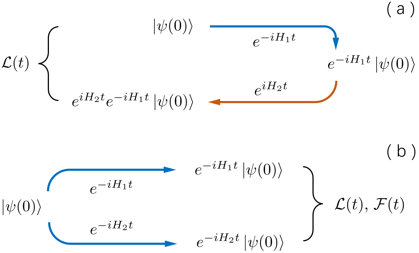
Figure 1: (a) $\mathcal{L}(t)$ defined as the overlap of the initial state $\ket{\psi(0)}$ with the state after the forward evolution under $H_{1}$ followed by the backward evolution under $H_{2}$ (Loschmidt echo). (b) $\mathcal{L}(t)$ obtained from the overlap of states of the forward evolutions from $\ket{\psi(0)}$ with $H_{1}$ and $H_{2}$, respectively (fidelity).

In the rotating frame with a common frequency, the one-dimensional $L$-qubit system studied in this work is governed, when including external drivings, by the 1D Bose-Hubbard model [6, 8]:

$$H(t)=H_{0}+H_{U}+\sum_{j=1}^{L}\omega_{j}(t)n_{j}+\frac{1}{2}\sum_{j=1}^{L}\Omega_{j}(a^{\dagger}_{j}+a_{j})~{},~{}$$ (2)

in which $H_{0}$ = $\sum_{j=1}^{L-1}J_{j,j+1}(a^{\dagger}_{j}a_{j+1}+\text{h.c.})$ is the hopping term with nearest neighbour coupling strength $J_{j,j+1}$ and $H_{U}$ = $\sum_{j=1}^{L}\frac{-U_{j}}{2}n_{j}(n_{j}-1)$ with the on-site interaction or anharmonicity $-U_{j}\leq 0$. $a^{\dagger}_{j}$ ($a_{j}$) is the bosonic creation (annihilation) operator and $n_{j}$ = $a^{\dagger}_{j}a_{j}$ is the number operator. The Hamiltonian in Eq. (2) includes a term of local transverse field with strength $\Omega_{j}$ written in the rotating frame of the driving frequency resonant with the qubit common frequency. The qubit frequency can also be tuned by ac magnetic flux in the form $\omega_{j}(t)=\varepsilon_{j}\cos(\nu t)$, with $\nu$ and $\varepsilon_{j}$ being the frequency and amplitude, respectively. In this case, without transverse field, $H(t)$ describes a Floquet system satisfying $H(t)=H(t+T)$ with a period of $T=2\pi/\nu$  [37]. In this work, we will consider three cases, namely, quenches with Floquet driving, without driving, and with transverse field, respectively. We will use constant coupling and field strengths $J$ and $\Omega$, and varying anharmonicity $U_{j}$ for individual qubits taken from experiments [16, 17], while the qubit next nearest neighbour coupling will be neglected (see the Supplemental Material [38]).

Note that the on-site interaction term $H_{U}$ will be absent if the system is populated only with one particle and the noncomputational high energy levels are not involved. The central goal of this work is to see the difference between the evolving quantum states with and without considering $H_{U}$ when high levels are only sparsely populated. For the experiment with time reversal, we can reverse the time evolution of the system in Eq.(2) by changing the signs of the coupling $J$, either directly via tunable coupler [39] or by Floquet driving [16, 17], and of the transverse field strength $\Omega$ by tuning the phase of driving field [40, 10], so that all terms in $H$ except $H_{U}$ change their signs. Therefore, $\mathcal{L}(t)$ describes the fidelity decay in a time reversed experiment that would be ignored if the two-level model is used, since in the model $H_{U}$ is absent giving rise to a perfect time reversal with fidelity of unity.

Without loss of generality, we consider the simple case in the absence of external drivings (Floquet and transverse field). The Loschmidt echo can be written as $\mathcal{L}(t)$ = $|\bra{\psi(0)}e^{i(H_{0}-H_{U})t}e^{-i(H_{0}+H_{U})t}\ket{\psi(0)}|^{2}$. The difference between the Hamiltonians of the forward (from $0$ to $t$) and backward (from $t$ to $2t$) evolution is $\Delta H$ = 2$H_{U}$. As explained above, by calculating Loschmidt echo $\mathcal{L}(t)$ in Fig. 1(a), we identically obtain the fidelity between two states evolving with Hamiltonians $H_{1,2}$ = $H_{0}\pm H_{U}$ as illustrated in Fig. 1(b). Since the timescale under consideration is well below the experimentally achievable coherence times (see SM [38]), dissipations are ignored in this work and evolutions of pure states are used in the numerical simulation. Namely, the Loschmidt echo $\mathcal{L}$ or the fidelity $\mathcal{F}$ can be calculated with pure states by $\mathcal{F}(t)=|\langle\psi(0)|\psi(t)\rangle|^{2}$, in which $\ket{\psi(t)}$ is the final state at $2t$. Or equivalently, $\mathcal{F}(t)=|\langle\psi_{1}(t)|\psi_{2}(t)\rangle|^{2}$, where $\ket{\psi_{1,2}(t)}$ = $e^{-iH_{1,2}t}\ket{\psi(0)}$ [41].

For the experiment with time evolution in one direction, we identically calculate $\mathcal{L}(t)$ for a forward evolution to time $t$ from a given initial state under $H_{0}$ in the Fock state site basis $\ket{n_{1},n_{2},...,n_{L}}$ with $n_{i}$ = 0, 1, and a backward evolution under $H_{1}$ = $H_{0}+H_{U}$ in the basis $\ket{n_{1},n_{2},...,n_{L}}$ with $n_{i}$ = 0, 1, …, $K-1$ ($K$ being the number of qubit levels considered). The basis for the states in the forward evolution is expanded to that in the backward evolution for the calculation. This is again equivalent to the time dependent overlap or fidelity decay between the two wave functions evolving from the same initial state to time $t$ under the two different Hamiltonians $H_{0}$ and $H_{1}$, which offers a proper estimate of the error in the two-level approximation of transmons for experiments with time evolution in one direction.

III Numerical results with time reversal

In this section, we present the results for a 10-qubit chain ($L$ = 10) with time reversal process in three different cases using typical experimental parameters of superconducting transmon qubits (see the Supplemental Material [38]). The calculations are performed using the QuTiP toolbox [42, 43] considering three energy levels ($K$ = 3) for each qubit. The high level therefore refers to the energy level of the qubit second-excited state. We will use the terms interchangeably. For more straightforward and convenient comparisons with the reported experiments, the time evolutions will be shown in nanoseconds and the normalized time $tJ/2\pi$ is used in the place required with which $tJ/2\pi$ = 1 corresponds to the time $t$ = 1 $\mu$s when $J/2\pi$ = 1 MHz.

III.1 Quench with Floquet driving

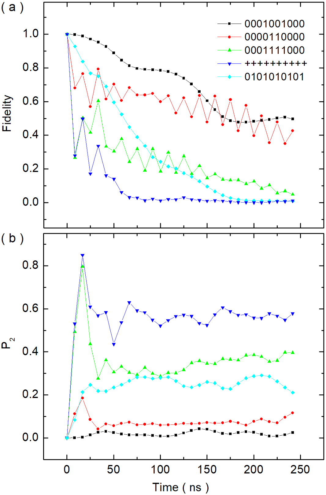
Figure 2: Time dependence of (a) fidelity and (b) total population of the second excited state during forward evolution. The initial states are $\psi_{1}$ = $\ket{0001001000}$, $\psi_{2}$ = $\ket{0000110000}$, $\psi_{3}$ = $\ket{0001111000}$, $\psi_{4}$ = $\ket{++++++++++}$, and $\psi_{5}$ = $\ket{0101010101}$. Time reversal is performed by Floquet driving. See text for the parameters used in the numerical calculations.

Periodically modulating many-body systems using sinusoidal or non-sinusoidal drive is a standard tool for the studies of gauge fields, topological band structures, phase transition [37], and nonequilibrium state of matter such as the discrete time-crystalline phase [44]. In Eq. (2), with $\nu\gg J$ and in the absence of $H_{U}$ and transverse field, we obtain a time-independent Hamiltonian $H_{\text{eff}}$ = $\sum_{j=1}^{9}J_{\text{eff}}(a^{\dagger}_{j}a_{j+1}+\text{h.c.})$ with $J_{\text{eff}}\approx J\mathcal{J}_{0}(\varepsilon/\nu)$, where $\mathcal{J}_{0}\big{(}x\big{)}$ is the Bessel function of order zero [37]. This is realized by driving the odd-number qubits with the same amplitude $|\varepsilon_{j}|=\varepsilon$ and staggered phase [16, 17]. $J_{\text{eff}}$ can thus be tuned from positive to negative by changing $\varepsilon$ and $\nu$ resulting in a time-reversible system $H_{\text{eff}}$.

In Fig. 2, we show the calculated time dependence of fidelity and total population of the qubit second-excited state $P_{2}$ = $\sum_{j=1}^{10}P_{2}^{j}$ ($P_{2}^{j}$ for the $j$th qubit) during forward evolution for five different initial states of $\psi_{1}$ = $\ket{0001001000}$, $\psi_{2}$ = $\ket{0000110000}$, $\psi_{3}$ = $\ket{0001111000}$, $\psi_{4}$ = $\ket{++++++++++}$, and the Néel state $\psi_{5}$ = $\ket{0101010101}$ ($\psi_{i}$ stands for $\ket{\psi_{i}(0)}$). Here $\ket{0}$ and $\ket{1}$ are the qubit ground and first-excited states, and $\ket{+}$ is the eigenstate of Pauli matrix $\sigma^{x}$ with eigenvalue of $+1$. In the calculations, we set $J/2\pi$ = 10.8 MHz and $U_{j}/2\pi$ around 212 and 264 MHz for odd and even number qubits, respectively [38]. Also, we fix $\nu/2\pi$ = 120 MHz, and the driving amplitude is $\varepsilon_{f}/2\pi=213.6$ MHz and $\varepsilon_{b}/2\pi=400$ MHz for the forward and backward evolutions, which lead to $\mathcal{J}_{0}(\varepsilon_{f}/\nu)=-\mathcal{J}_{0}(\varepsilon_{b}/\nu)$ corresponding to $J_{\text{eff}}/2\pi$ $\approx\pm 3.8$ MHz. All the data are collected in a stroboscopic fashion in the step of the driving period $2\pi/\nu$ $\approx$ 8.33 ns [37].

We choose five different initial states to see their different influence on the fidelity decay. $\psi_{1}$ and $\psi_{2}$ have the total particle number $N$ = 2 (note $N$ is conserved), but they have different particle distributions. $\psi_{3}$, $\psi_{5}$, and $\psi_{4}$ have $N$ = 4, $N$ = 5, and an expectation value of 5, respectively. In Fig. 2, we find a general trend that fidelity decays faster with the increase of $N$ that results in the increase of high level excitations. An initially fast rising of the excitations leads to fast dropping of the fidelity. In addition, the spatial separation of particles will cause the process less abrupt, as can be seen from the comparison of the data between $\psi_{1}$, $\psi_{5}$ and $\psi_{2}$, $\psi_{3}$, $\psi_{4}$. Detailed results of the population variations with time for individual qubits, during both the forward and backward evolutions can be found in the Supplemental Material [38]. There it is seen that in the cases of $\psi_{2}$ and $\psi_{3}$ the populations in the qubit high level tend to remain in the initially excited qubits which locate next to each other. This is not the case when they are separated, as in the case of $\psi_{1}$.

III.2 Quench without driving

Figure 3 shows the results for the same initial states in the cases without Floquet driving and transverse field. The time reversal is implemented by directly changing the sign of qubit coupling $J$ in the numerical calculations. In the main panels with $J/2\pi$ = 16 MHz, one can again see the more significant fidelity decay with increasing $N$, but the fidelities in the cases of $\psi_{1}$ and $\psi_{2}$ become almost the same although their high-level excitations are clearly different. The difference as compared to the results in Fig. 2 may result from some detailed processes which are presently unclear. In the Supplemental Material [38], it can also be seen that the populations in the qubit high level tend to remain in the initially excited qubits when located next to each other.

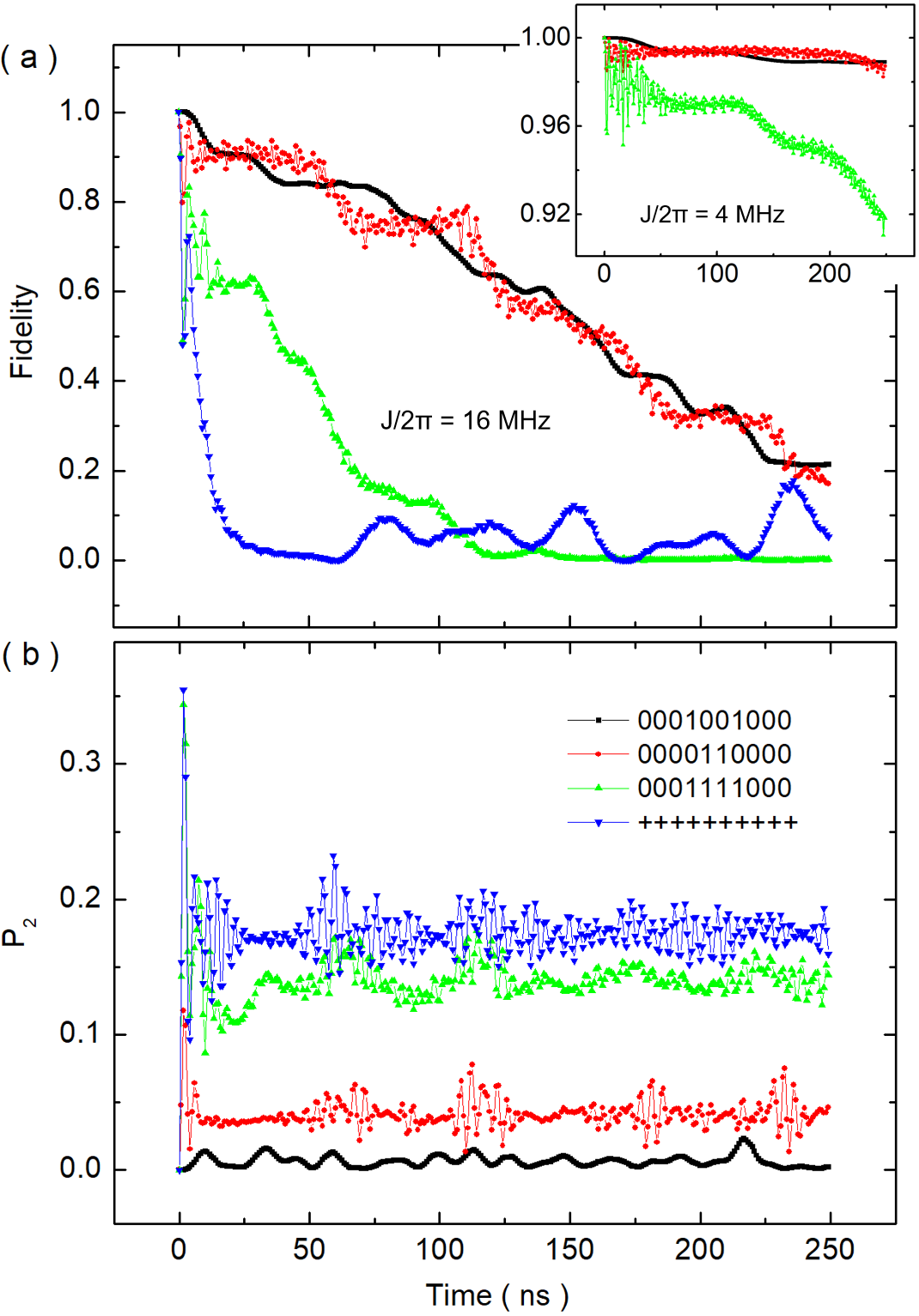
Figure 3: Time dependence of (a) fidelity and (b) total population of the second excited state during forward evolution without external driving. The initial states are $\psi_{1}$ = $\ket{0001001000}$, $\psi_{2}$ = $\ket{0000110000}$, $\psi_{3}$ = $\ket{0001111000}$, and $\psi_{4}$ = $\ket{++++++++++}$. Time reversal is performed by changing the sign of the coupling strength $J$, which is 2$\pi\times$16 and 2$\pi\times$4 MHz in the main panels and inset, respectively.

An important observation from the numerical simulations is that the fidelity decay strongly depends on the qubit coupling strength $J$ as well as on the configuration of the initial state. This is expected since reducing $J$ leads to an increasing ratio $U/J$ while the hard-core boson model is arrived when $U/J$ $\rightarrow$ $\infty$ [25]. The inset of Fig. 3 shows the results for $\psi_{1}$, $\psi_{2}$, and $\psi_{3}$ with a reduced $J/2\pi$ of 4 MHz, as compared to the data with $J/2\pi$ = 16 MHz in the main panels. The corresponding results for $\psi_{4}$ are presented separately in Fig. 4(a). In the inset of Fig. 3, the fidelity only shows a slight decrease for $\psi_{1}$ and $\psi_{2}$, a moderate decrease for $\psi_{3}$, but a significant decay for $\psi_{4}$ as shown in Fig. 4(a). In the cases of $\psi_{2}$ and $\psi_{3}$, the populations at high level are on the order of 0.1$\%$ and 0.2$\%$ for the initially excited qubits, respectively, and the values for the other qubits and those for all qubits in the case of $\psi_{1}$ are negligible. Looking at the populations in the first-excited state of the initially excited qubits in these cases, we find that they almost return to unity ($\sim$0.994, 0.992, and 0.974 for $\psi_{1}$, $\psi_{2}$, and $\psi_{3}$, respectively) at the end of the time reversal process (see the Supplemental Material [38]).

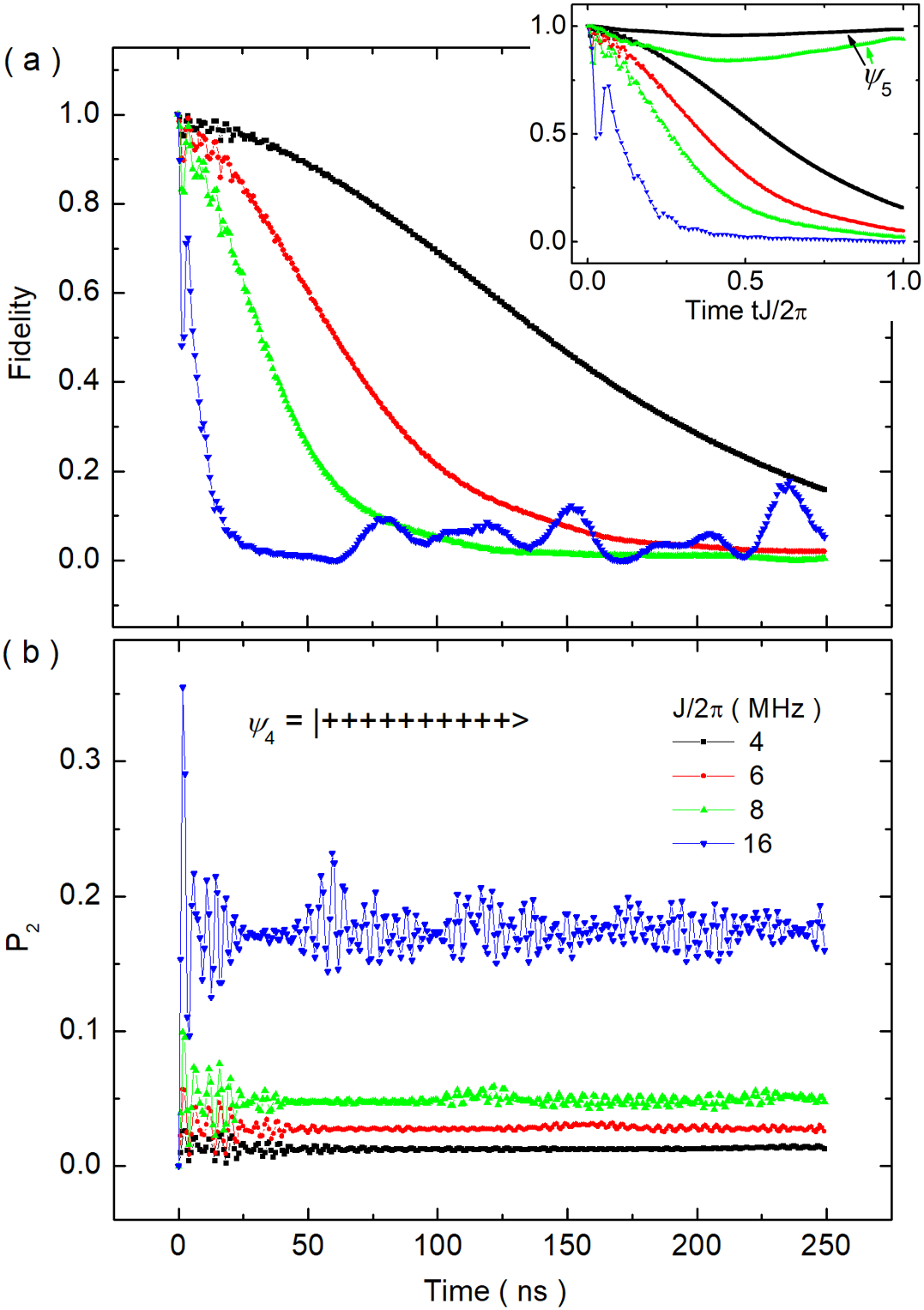
Figure 4: Time dependence of (a) fidelity and (b) total population of the second excited state during forward evolution without external driving. The initial state is $\psi_{4}$ = $\ket{++++++++++}$ and different $J/2\pi$ = 4, 6, 8, and 16 MHz are used. Time reversal is performed by changing the sign of $J$. The inset shows the fidelity against time $tJ/2\pi$ with two additional results for Néel state $\psi_{5}$ = $\ket{0101010101}$ with $J/2\pi$ = 4 and 8 MHz.

The fidelity decay and total population versus time for several different $J$ are presented in Fig. 4 for the case of $\psi_{4}$. The results demonstrate a fast decay rate increase as $J$ increases. To subtract the factor of the increase of $J$, which measures the time of hopping process, the decay rate increase is still substantial, as can be seen in the inset of Fig. 4 plotted against $tJ/2\pi$. These results indicate strong influence of the qubit coupling strength on the fidelity decay in the QQD experiments. As can be seen in Figs. 2 and 3, the decay rate also depends on the initial state. In the inset of Fig. 4, we show two additional results for the Néel initial state $\psi_{5}$ = $\ket{0101010101}$ with $J/2\pi$ = 4 (solid line) and 8 (dashed line) MHz. It can be seen that for the Néel state with qubits initially excited on every other site, the decay rate decreases substantially in the regime of small $J$ and the state leakage to the qubit high level becomes negligible.

Comparing the data in Fig. 2 with $J/2\pi$ = 10.8 MHz and $J_{\text{eff}}/2\pi$ $\approx 3.8$ MHz to those in Figs. 3 and 4, we find that in the case of Floquet driving, the degrees of the fidelity decay and high-level population are more related to the qubit actual coupling strength than to the effective one, since for the case without driving the coupling strength $J/2\pi$ = 4 MHz leads to a fidelity decay much less severe.

III.3 Quench with transverse field

The application of a transverse field leads to the last term in Eq. (2) and changes the system from integrable to nonintegrable. The particle conservation is broken in this case. These give rise to many interesting phenomena which have been studied recently with superconducting circuits [10, 12]. In Fig. 5, we show the time dependence of fidelity and total population of the second-excited state for two initial states $\psi_{4}$ and $\psi_{5}$ with two different sets of coupling strength $J$ and transverse field $\Omega$. Again we see that the fidelity decay rate decreases quickly with decreasing $J$. The results also show opposite trends of decay rates for $\psi_{4}$ and $\psi_{5}$ as compared to the data in Fig. 4. Namely, although the populations in the second-excited state are larger for the $\psi_{4}$ state than that for the $\psi_{5}$ state with the same $J$ and $\Omega$, the fidelity decays more significantly for the Néel state $\psi_{5}$ than for the $\psi_{4}$ state. These are apparently contrary to the results in Fig. 4.

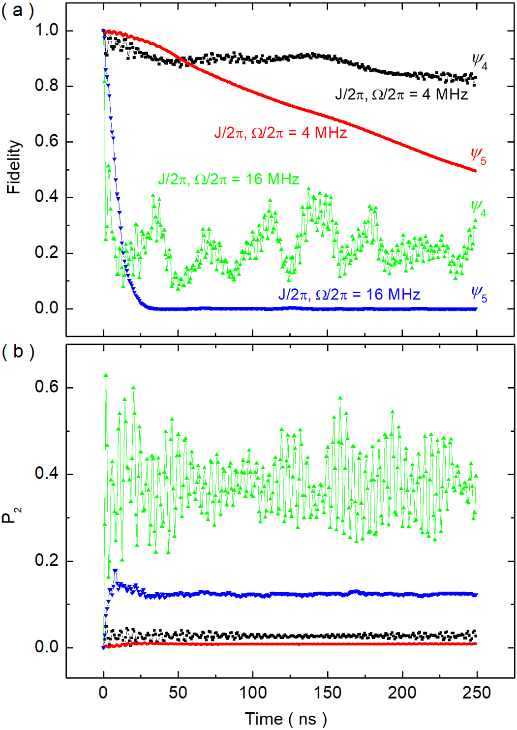
Figure 5: Time dependence of (a) fidelity and (b) total population of the second excited state during forward evolution with applied transverse field and two initial states $\psi_{4}$ = $\ket{++++++++++}$ and $\psi_{5}$ = $\ket{0101010101}$ for different coupling and field strengths $J$ and $\Omega$. Time reversal is performed by changing the signs of $J$ and $\Omega$.

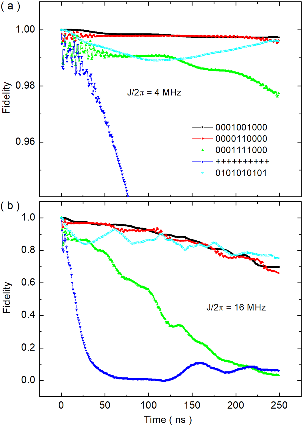
Figure 6: Time dependence of fidelity with (a) $J/2\pi$ = 4 MHz and (b) $J/2\pi$ = 16 MHz for the initial states $\psi_{1}$ = $\ket{0001001000}$, $\psi_{2}$ = $\ket{0000110000}$, $\psi_{3}$ = $\ket{0001111000}$, $\psi_{4}$ = $\ket{++++++++++}$, and $\psi_{5}$ = $\ket{0101010101}$. The evolutions are in a single forward direction without external driving.

The fact that the decay rate becomes higher for $\psi_{5}$ than that for $\psi_{4}$ may relate in a complicated way to the interplay of the high-level excitation and the well-known process of thermalization in nonintegrable chaotic systems with applied transverse field [45, 12]. Specifically, for the results in Fig. 5 the system can be identified as chaotic, and strong and weak thermalizations occur for the initial states of $\psi_{5}$ and $\psi_{4}$, respectively. In the Supplemental Material [38], we show their distinct behaviours of the entanglement entropy in the forward and backward evolution directions. Also, we find that for the Néel state $\psi_{5}$ with $J/2\pi$ = $\Omega/2\pi$ = 16 MHz, the populations of the first-excited state $P_{1}$ for each qubit will oscillate and approach around 0.5 in a timescale of $\sim$100 ns. An interesting observation is that the populations of each qubit stay around 0.5 afterwards and do not show any sign of changing back even when the time reversal process is performed. A population of 0.5 corresponds to a zero expectation value of $\sigma^{z}$. In this strongly thermalized regime, the expectation values of other Pauli matrices will only have small-magnitude oscillations around zero. This means that the Bloch vector of each qubit progressively shrinks in the thermal state and does not change back afterwards [46]. Such a feature of local operators is consistent with that of the entanglement entropy in the Supplemental Material [38]. Considering the identical view in Fig. 1(b) with two wave functions evolving in the same forward direction, the results imply that thermalization generally aggravates the fidelity decay in the QQD experiment with high-level participation.

Without high-level populations, the system is described by a two-level model and can have a perfect time reversal with unity fidelity also in the thermalized state. For the Néel state with $J/2\pi$ = $\Omega/2\pi$ = 4 MHz and small high-level populations, partly reversed processes are found from population $P_{1}$ as well as entanglement entropy. The situation is quite different in the weakly thermalized regime for the $\psi_{4}$ initial state, as indicated by the entanglement entropy in the Supplemental Material [38]. The expectation value of $\sigma^{x}$ will oscillate around finite values while those of the other Pauli matrices around zero with moderate amplitudes. Compared with the data in Fig. 4, the results in Fig. 5 shows larger high-level populations but a smaller fidelity decay for the initial state $\psi_{4}$, which remains to be explained.

IV Numerical results with time evolution in one direction

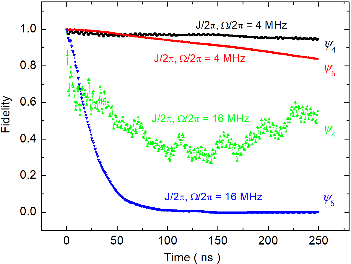
Figure 7: Time dependence of fidelity with applied transverse field and two initial states $\psi_{4}$ = $\ket{++++++++++}$ and $\psi_{5}$ = $\ket{0101010101}$ for different coupling and field strengths $J$ and $\Omega$. The evolutions are in a single forward direction.

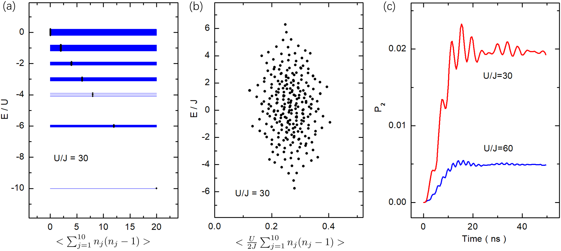
Figure 8: Simple particle conserved system $H$ = $H_{0}+H_{U}$ of the 10-qubit chain. (a) Energy levels forming bands with $U/J$ = 30 and $N$ = 5. The black dots show the expectation values $A$ of the anharmonicity operator $\sum_{j=1}^{10}n_{j}(n_{j}-1)$. (b) Enlarged plot of the expectation values of the anharmonicity operator in the top band showing the eigenvalues in unit of $J$ against $(U/2J)A$. (c) Total population of the second-excited state in the transitional stage right after quenching of the system for the Néel initial state $\psi_{5}$ with $J/2\pi$ = 8 MHz, and $U/2\pi$ = 240 (upper curve) and 480 (lower curve) MHz.

Many QQD experiments using superconducting circuits are performed with quantum state evolution in a single forward direction [7, 8, 10, 11, 12, 13, 15]. In Figs. 6 and 7, we show the numerical results without the time reversal process, which correspond to the data in Figs. 3, 4, and 5 with time reversal. It can be seen that the general trends are the same for the two situations. In particular, for larger coupling strength $J/2\pi$ = 16 MHz, the fidelity decay rates are almost identical if twice the total time duration in the time reversed situation is considered. However, with $J/2\pi$ = 4 MHz, the fidelity appears to decay faster in the time reversed situation after considering the twice time duration. This is generally understandable since in this case the two quantum states evolve from the same initial state under $H_{1}$ and $H_{2}$ (or both plus the transverse field term) with different terms $\pm H_{U}$ of opposite signs. Therefore the fidelity decay rate is larger compared to the situation with time evolution in one direction in which the states evolve under $H_{0}$ and $H_{1}$ (or both plus the transverse field term) with the term $H_{U}$ appearing only in $H_{1}$.

V Discussions

In a QQD experiment, individual qubits in the multiqubit system are first biased at their respective idle frequencies, where they are essentially decoupled, to prepare a ground, excited, superposition, or entangled state. With these constituting the initial state, the qubits are biased at the quench time $t$ = 0 to the same resonant working frequency at which a particular Hamiltonian $H(t)$ in Eq. (2) is used for the system evolution. Finally, all qubits are set back to their idle frequencies and the state of each qubit is measured tomographically. Physically, before $t$ = 0, the decoupled qubit system can be described via the Fock state site basis $\ket{n_{1},n_{2},...,n_{L}}$ with a Hilbert space dimension of $K^{L}$ when the number of levels $K$ is considered for each qubit. However, only the bottom two levels are used for the initial state construction and all the high levels are unoccupied. At $t$ = 0, the initial state can be expanded in terms of the eigenbasis of $H$ with the same Hilbert space dimension. The state will then evolve according to Schrödinger’s equation, producing high-level populations which can be measured when the qubits are brought back to the idle points and the evolved state is expressed in Fock state site basis again.

V.1 Process at the initial stage after quench

For the present case of positive $J$ and negative $-U$ in the Hamiltonian $H(t)$ in Eq. (2), the system has mostly negative eigenvalues with zero energy near the top of the energy spectrum, and the total energy of the initial states considered in this work is (near) zero. As a concrete example, we consider the simple particle conserved system $H$ = $H_{0}+H_{U}$ of the 10-qubit chain with the Néel initial state and constant $J/2\pi$ = 8 MHz, $U/2\pi$ = 240 MHz for all qubits corresponding to $U/J$ = 30. For this system, the eigenvalue problem can be accurately solved in the $N$-particle block of Hamiltonian matrix with $K$ = $N+1$ levels for each qubit. The block, or the Hilbert space dimension is $(N+L-1)!/(L-1)!/N!$ for the $L$-qubit chain, which equals 2002 for $L$ = 10 and the Néel initial state with $N$ = 5. In Fig. 8(a), we show the energy spectrum calculated using the QuSpin package [47, 48]. The black dots in the figure are the expectation values of the anharmonicity operator $A$ = $<\sum_{j=1}^{10}n_{j}(n_{j}-1)>$. For the present large value of $U/J$ = 30, the spectrum clearly shows the band structure with band separation in unit of $U$ and grouped by different values of $A$. In Fig. 8(b), we replot $A$ in the top band in which the lift of the eigenvalue degeneracy on the order of the coupling strength $J$ can be seen [49, 50].

The upper curve in Fig. 8(c) shows the temporal variation of the total population of the second-excited state after the system quench at $t$ = 0, with the same parameters of $J$ and $U$ described above. The lower curve is the result with increased $U/2\pi$ = 480 MHz and $U/J$ = 60. We see that doubling $U/2\pi$ roughly reduces the second-excited state population to a quarter of the value after the transitional period. In addition, the two curves show well defined oscillations with a frequency equal to $U/2\pi$, which are more prominent at the beginning after quench. This can be explained by the results in Fig. 8(a). In the $N$ = 5 system, the lowest energies in the figure correspond to the configurations of all five particles residing in the same qubit thus leading to $A$ $\sim$ 20. On the other hand, in the top band each qubit has no more than one particle, while in the second band from the top, only one qubit is allowed to have increased two particles, leading to the nonzero population in the second excited state. The total energy of the system is zero and does not change with time. Therefore, the system has the largest probability in the eigenstates in the top band and the oscillations in the figure reflect the separation of the top bands. The corresponding oscillations in fidelity with the same frequency of $U/2\pi$ as in the second-excited state population, which can be seen in Figs. 3 to 7, provides a clear indication that the fidelity is influenced by the presence of the qubit high level.

We have used three energy levels for each qubit ($K$ = 3) in our numerical simulations in the previous sections. The results are accurate in the cases of the initial states $\psi_{1}$ and $\psi_{2}$ with $N$ = 2. For the other initial states, the calculation should be approximate. For the results in Fig. 8(a), there will be only three top bands left if we use three levels for each qubit in stead of six levels in the calculation. We find that the deviations of both the eigenvalues and expectation values of the anharmonicity operator such as the data in Fig. 8(b) are small by using three and six levels in the calculation, and those for the top band are smallest. Since for the Néel initial state the system has zero total energy, it has the probabilities in the eigenstates orders of magnitude smaller when going from the top band to the lower bands, so that the level structure of the top band basically determines the system property during evolution. As a result, numerical simulations using three levels for each qubit are expected to be a good approximation.

V.2 Comparison with experiment

We now compare our numerical results with some of the QQD experiments using superconducting transmon qubits [7, 8, 10, 11, 12, 14, 15, 16, 17].

Strongly correlated quantum walks have been studied with adjacently and separately placed two photons in a 12-qubit superconducting processor [8]. The fermionization of strongly interacting photons and the antibunching of photons with attractive interactions have been observed, which is described by the hard-core boson model in good approximation. The superconducting processor has the parameters of $J/2\pi$ $\sim$ 12 MHz, and two sets of $U/2\pi$ $\sim$ 200 and 240 MHz for the even and odd site qubits, respectively. The situation is similar to those discussed in Figs. 3 and 6 for the initial states of $\psi_{1}$ and $\psi_{2}$ with similar $U/2\pi$ and an intermediate $J/2\pi$ between 16 and 4 MHz. The populations of the second-excited state for individual qubits are discussed in Ref. [8], which can be seen in more detail with present parameters in the Supplemental Material [38] together with the total population in Fig. 3(b).

The many-body localization phenomenon arising from the interplay between interaction and disorder has been observed in a superconducting circuit with all-to-all connectivity [7]. The ordered Néel initial state $\ket{0101010101}$ is prepared, and the system is found to have a uniform population of 0.5 for all qubits at the end of the state evolution in the absence of disorder. However, in strong disorder the system maintains the population distribution of the initial state. These experimental results are found to be well described by the two-level spin model. The superconducting processor has a very small coupling strength $J/2\pi$ below 2 MHz and an on-site interaction $U/2\pi$ around 240 MHz. From the results in the inset of Fig. 4 and in Fig. 6, we can see that the fidelity decay should become insignificant, with the populations of the qubit second-excited state safely negligible.

The out-of-time-order correlator (OTOC) is an important tool to study the dynamics of quantum many-body systems. In Ref. [14], a 3$\times$3 two-dimensional lattice of superconducting qubits is implemented to study the time-reversibility, measurement of OTOC, propagation of quantum information, and many-body localization in the presence of frequency disorder. The experiment is found to be fairly described by the hard-core boson model in the time range of $\sim$100 ns with $J/2\pi$ = 8.1 MHz and $U/2\pi$ = 244 MHz. The initial states with one, two, and three excited particles in the 9-qubit lattice are similar with the present $\psi_{1}$, $\psi_{2}$, and $\psi_{3}$ in one dimension. In particular, the error of the OTOC (or equivalently the commutator) caused by the qubit high level is carefully estimated considering the $ZZ$ interaction in both cases of the 3$\times$3 lattice and a 7-qubit chain [14]. It is found that the error would grow linearly with time, and in the cases of the initial states with filled particle number ranging from two to five, the time for reliable results is around a few hundreds to tens of ns for both the lattice and chain. These estimations from the commutator, with somewhat different $U/J$ and the ratio of particle to qubit numbers, are comparable to the data in Figs. 3 and 6 from the fidelity calculations.

In a recent experiment with a superconducting 10-qubit chain, the time reversal of the system is realized by using Floquet driving and the OTOCs are successfully measured [16]. The sample parameters are listed in the Supplemental Material [38]. The experimental results show distinct behaviours with and without a signature of information scrambling in the near integrable system for the butterfly operators of $\sigma_{x}$ and $\sigma_{z}$, respectively. For the measurements in the two cases, the initial states of $\psi_{4}$ = $\ket{++++++++++}$ and $\psi_{5}$ = $\ket{0101010101}$ are prepared. It is found that to well describe the experimental results, the consideration of three qubit levels is necessary for $\psi_{4}$ while the two-level model modified with $ZZ$ interaction can be used for $\psi_{5}$. Such difference is reasonable from the data in Fig. 2 (also the inset of Fig. 4) considering that the fidelity decays faster for $\psi_{4}$ than for $\psi_{5}$ with the other parameters unchanged. The failure of the simple two-level approximation is also expected since the fidelity decreases almost to zero in the timescale of the experiment (consideration of next nearest neighbour coupling will bring a small change). As is discussed in section III, the fidelity decay with Floquet driving is basically governed by the qubit actual coupling strength $J/2\pi$ = 10.8 MHz, which is much larger than the effective coupling strength $J/2\pi$ = $\pm$3.8 MHz that determines the experimental timescale. In addition, the fidelity in some cases shows a clear decrease while the population almost returns to the initial values at the end of time evolution. This indicates a more precise measure of fidelity than that of population [41, 26]. In the OTOC experiment with $\sigma_{z}$ butterfly operator and Néel initial state [16], the final measurement is the expectation value of $\sigma_{z}$, which is equivalent to the qubit population.

Finally, we mention two experiments in the presence of transverse field with superconducting circuits [10, 12]. In one experiment, dynamical phase transitions in the two-level Lipkin-Meshkov-Glick model are observed with 16 all-to-all connected superconducting qubits [10]. The sample has a small mean value of the coupling strength $J/2\pi$ = 1.45 MHz and an on-site interaction $U/2\pi$ around 240 MHz, for which negligible fidelity decay is expected. In another experiment, strong and weak thermalization is observed for different initial states fully polarized or located on the equator of the Bloch sphere, which is described by the two-level spin model considering the $Z$- and $XY$-crosstalk induced disorders in chemical potential and local transverse field [12]. The coupling strength $J/2\pi$ and on-site interaction $U/2\pi$ of the sample are around 13 MHz and 235 MHz, respectively. Generally, the fidelity decay for the initial state on the equator should be less affected by the high-level participation with applied transverse field, as is shown in Figs. 5 and 7. However, the comparison with the present numerical simulation is not straightforward due to the two kinds of disorders existed in the experiment.

VI Summary and outlook

Fidelity is a standard and precise measure of the distance between quantum states [41, 26], which was used to investigate the accuracy and validity of the two-level approximation for the multilevel transmons in the QQD experiments. In order to evaluate the effect of the high energy levels of transmon qubits, the fidelity decay (i.e., the time dependent overlap of wave functions) was calculated for two experimental situations with and without time reversal process and for a number of system Hamiltonians and initial states. Our results showed that the qubit high-level populations may lead to remarkable fidelity decay during state evolution in a QQD experiment, depending on the ratio $U/J$, the initial states, and the applied driving. In many cases, it is seen that the ratio of $U/J$ should roughly be larger than $\sim$ 60 for safely neglecting the high-level populations created in the quench process in a timescale of 2$\pi/J$. For the usual transmon qubits with $U/2\pi$ $\sim$ 240 MHz, for instance, the qubit coupling strength $J/2\pi$ should be $\sim$ 4 MHz and below for a simulation experiment with time evolution up to $\sim$ 250 ns. The criterion is nevertheless relative and under these conditions, the fidelity generally remained above 0.9 and the high-level population for individual qubits was well below 0.01 in most cases. Furthermore, our results showed that the fidelity decay also depends on the initial state and system Hamiltonians applied with external drivings. These factors need to be taken into account for the application of the two-level spin and hard-core boson models in the QQD experiments.

Various many-body quantum phenomena have been studied and successfully demonstrated in a number of QQD experiments using transmon qubits with sufficiently low high-level populations [7, 8, 10, 11, 12, 14, 15]. The key parameter for the applicability of the two-level approximation for transmons is the ratio $U/J$ since the ideal hard-core boson model is achieved when $U/J$ tends to infinity. From the above discussions, satisfactory approximations can be made experimentally taking advantage of the present-day technologies of device design and fabrication. In particular, we mention the strong anharmonicity or high $U$ devices such as capacitively shunted qubits, which have become available [51, 52] and may offer a convenient playground in the future for the study of the spin and hard-core boson models using superconducting circuits.

Supplemental Material for
``Two-level approximation of transmons in quantum quench experiments"

This Supplemental Material includes one table and twelve figures, which are explained below.

I. Consideration of model parameters for numerical simulations

In Table S1, we list the relevant device parameters of a ten transmon qubit chain from Ref. [1] for the consideration of our model parameters for numerical simulations. These parameters are typical and often seen in the QQD experiments using superconducting qubits [2, 3]. For transmon qubits, the coherence times are much longer than the time scales of interest in this work, so dissipations are not taken into account in our simulation. We note that the anharmonicity $-U_{j}/2\pi$ given in the table is around $-212$ and $-264$ MHz for odd and even number qubits, respectively (a negative sign is given explicitly for the anharmonicity so we have a positive $U_{j}$ for the convenience of discussion). These anharmonicity parameters are used for all calculations in this work except for the results of Fig. 8 discussed in Sec. V A of the main text. Generally, a more smooth or constant $U_{j}/2\pi$ tends to slightly increase the fidelity decay rate. On the other hand, an averaged $uniform$ nearest-neighbour (NN) coupling strength $J/2\pi$ = 10.8 MHz is used for simplicity in the simulation of Floquet driven system. In this case, the driving parameters are such that the forward and backward state evolutions have the effective coupling strengths of 3.8 and -3.8 MHz, respectively. Uniform NN couplings with varying strength are also used for the simulations in other situations.

II. Detailed population variations of individual qubits

In Fig. S1 through Fig. S9, we show the detailed time dependence of populations for individual qubits during both the forward and backward evolutions. Figs. S1 to S3, Figs. S4 and S5, Figs. S6 and S7, and Figs. S8 and S9 are the data corresponding to the cases in Fig. 2, Fig. 3 (inset), Fig. 4, and Fig. 5 in the main text, respectively. The detailed population variations with time of the second-excited state for weak coupling strength $J/2\pi$ = 4 MHz are shown separately in Fig. S10 and Fig. S11 due to their much smaller values.

III. Entanglement entropy

The entanglement entropies corresponding to the data in Fig. 5 in the main text are shown in Fig. S12.

Table S1: Typical transmon qubit device parameters [1] considered for numerical simulations in this work, where $-U$ is the qubit anharmonicity and $J_{j,j+1}$ is the coupling strength between the nearest-neighbour (NN) qubits Q_j and Q_j+1.

	Q1	Q2	Q3	Q4	Q5	Q6	Q7	Q8	Q9	Q10
$-U/2\pi$ (MHz)	-212	-264	-210	-268	-212	-268	-214	-264	-214	-264
$J_{j,j+1}/2\pi$ (MHz)	10.72        10.73        10.99        11.05        10.88        10.48        10.86        10.79        10.78

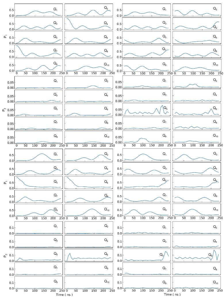
Figure S1: Detailed population variations of individual qubits for the results in Fig. 2 with Floquet driving and initial states of $\ket{0001001000}$ (upper four panels) and $\ket{0000110000}$ (lower four panels). The left and right columns are the forward and backward evolutions, while the odd and even rows are for the first- and second-excited states, respectively.

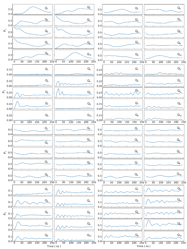
Figure S2: Detailed population variations of individual qubits for the results in Fig. 2 with Floquet driving and initial states of $\ket{0001111000}$ (upper four panels) and $\ket{++++++++++}$ (lower four panels). The left and right columns are the forward and backward evolutions, while the odd and even rows are for the first- and second-excited states, respectively.

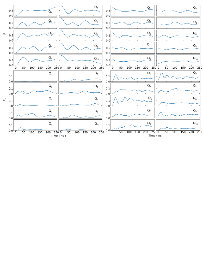
Figure S3: Detailed population variations of individual qubits for the results in Fig. 2 with Floquet driving and initial states of $\ket{0101010101}$. The left and right columns are the forward and backward evolutions, while the upper and lower panels are for the first- and second-excited states, respectively.

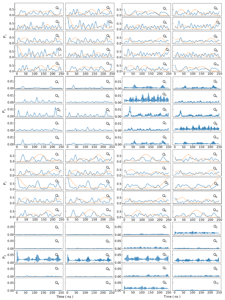
Figure S4: Detailed population variations of individual qubits for the results in Fig. 3 (solid lines) with NN coupling of 16 MHz and initial states of $\ket{0001001000}$ (upper four panels) and $\ket{0000110000}$ (lower four panels). The left and right columns are the forward and backward evolutions, while the odd and even rows are for the first- and second-excited states, respectively. Dashed lines correspond to those in the inset of Fig. 3 with NN coupling of 4 MHz.

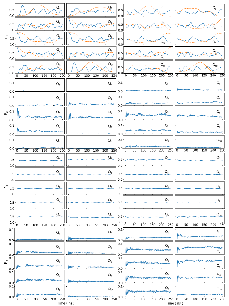
Figure S5: Detailed population variations of individual qubits for the results in Fig. 3 (solid lines) with NN coupling of 16 MHz and initial states of $\ket{0001111000}$ (upper four panels) and $\ket{++++++++++}$ (lower four panels). The left and right columns are the forward and backward evolutions, while the odd and even rows are for the first- and second-excited states, respectively. Dashed lines correspond to those in the inset of Fig. 3 with NN coupling of 4 MHz.

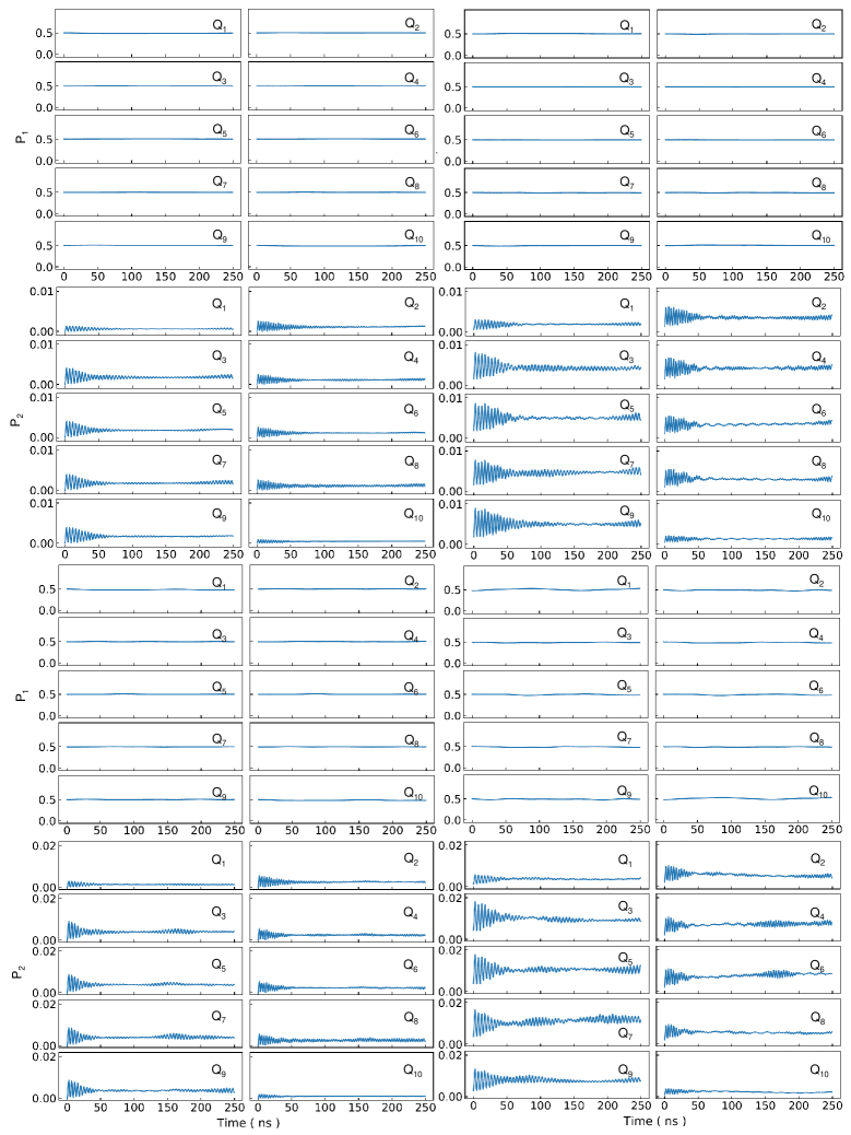
Figure S6: Detailed population variations of individual qubits for the results in Fig. 4 with initial state $\ket{++++++++++}$ and NN coupling of 4 MHz (upper four panels) and 6 MHz (lower four panels). The left and right columns are the forward and backward evolutions, while the odd and even rows are for the first- and second-excited states, respectively.

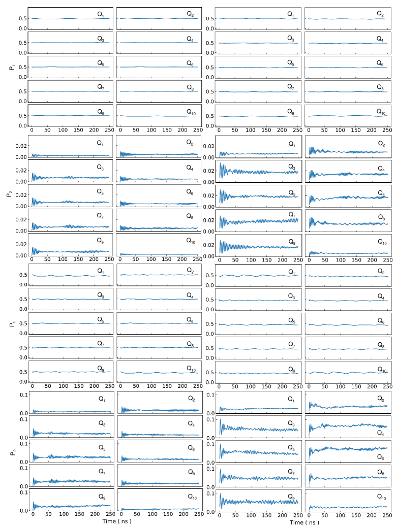
Figure S7: Detailed population variations of individual qubits for the results in Fig. 4 with initial state $\ket{++++++++++}$ and NN coupling of 8 MHz (upper four panels) and 16 MHz (lower four panels). The left and right columns are the forward and backward evolutions, while the odd and even rows are for the first- and second-excited states, respectively.

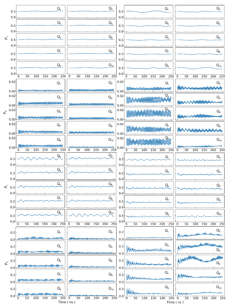
Figure S8: Detailed population variations of individual qubits for the results in Fig. 5 with initial state $\ket{++++++++++}$. The NN coupling and transverse field strength are 4 and 4 MHz in upper four panels, and 16 and 16 MHz in lower four panels. The left and right columns are the forward and backward evolutions, while the odd and even rows are for the first- and second-excited states, respectively.

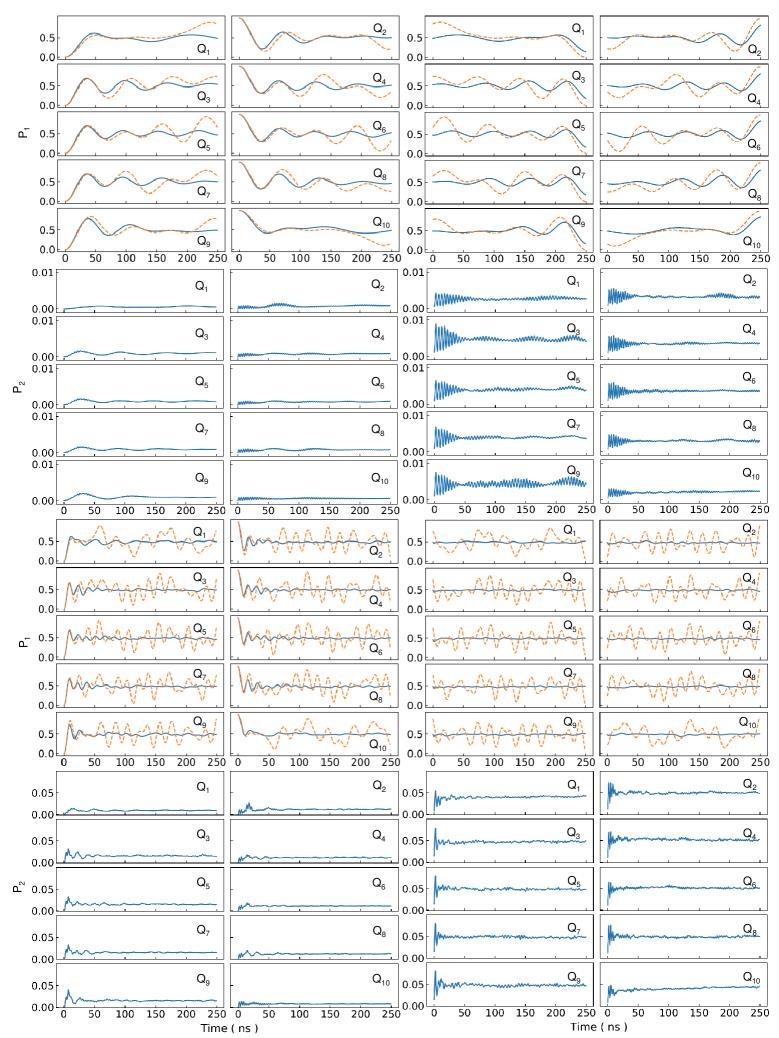
Figure S9: Detailed population variations of individual qubits for the results in Fig. 5 with initial state $\ket{0101010101}$. The NN coupling and transverse field strength are 4 and 4 MHz in upper four panels, and 16 and 16 MHz in lower four panels. The left and right columns are the forward and backward evolutions, while the odd and even rows are for the first- and second-excited states, respectively. The dashed lines are the corresponding results without transverse field.

Figure S10: Time dependence of total populations of the second-excited state with $J/2\pi$ = 4 MHz for (a, b) $\psi_{1}$, $\psi_{2}$, and $\psi_{3}$, (c, d) $\psi_{4}$ and $\psi_{5}$. In (a, c) and (b, d) are the forward and backward evolutions, respectively.

Figure S11: Detailed population variations of the second-excited state for individual qubits with $J/2\pi$ = 4 MHz for (a, b) $\psi_{1}$, $\psi_{2}$, and $\psi_{3}$, (c, d) $\psi_{4}$ and $\psi_{5}$. In (a, c) and (b, d) are the forward and backward evolutions, respectively. All curves have a one-to-one correspondence to those in Fig. S10 with the same colour.

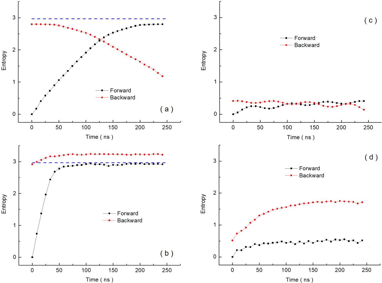
Figure S12: Entanglement entropies (of half-chain subsystem) corresponding to the data in Fig. 5 (see also Figs. S8 and S9), with initial states $\ket{0101010101}$ in (a) and (b), and $\ket{++++++++++}$ in (c) and (d). The parameters $J/2\pi$ and $\Omega/2\pi$ are 4 MHz for (a) and (c), and 16 MHz for (b) and (d). Dashed lines in (a) and (b) are the Page value $S^{Page}$ = [10ln(2)-1]/2 for the 10-qubit chain.

References

- [1] I. M. Georgescu, S. Ashhab, and F. Nori, Quantum simulation, Rev. Mod. Phys. 86, 153 (2014).
- [2] E. Altman, K. R. Brown, G. Carleo, L. D. Carr, E. Demler, C. Chin, B. DeMarco, S. E. Economou, M. A. Eriksson, K.-M. C. Fu et al., Quantum Simulators: Architectures and Opportunities, PRX Quantum 2, 017003 (2021).
- [3] A. J. Daley, I. Bloch, C. Kokail, S. Flannigan, N. Pearson, M. Troyer, and P. Zoller, Practical quantum advantage in quantum simulation, Nature 607, 667 (2022).
- [4] A. Polkovnikov, K. Sengupta, A. Silva, and M. Vengalattore, Nonequilibrium dynamics of closed interacting quantum systems, Rev. Mod. Phys. 83, 863 (2011).
- [5] J. Koch, T. M. Yu, J. Gambetta, A. A. Houck, D. I. Schuster, J. Majer, Alexandre Blais, M. H. Devoret, S. M. Girvin, and R. J. Schoelkopf, Charge-insensitive qubit design derived from the Cooper pair box, Phys. Rev. A 76, 042319 (2007).
- [6] P. Roushan, C. Neill, J. Tangpanitanon, V. M. Bastidas, A. Megrant, R. Barends, Y. Chen, Z. Chen, B. Chiaro, A. Dunsworth, A. Fowler, B. Foxen, M. Giustina, E. Jeffrey, J. Kelly, E. Lucero, J. Mutus, M. Neeley, C. Quintana, D. Sank, A. Vainsencher, J. Wenner, T. White, H. Neven, D. G. Angelakis, and J. Martinis, Spectroscopic signatures of localization with interacting photons in superconducting qubits, Science 358, 1175 (2017).
- [7] K. Xu, J. J. Chen, Y. Zeng, Y. -R. Zhang, C. Song, W. X. Liu, Q. J. Guo, P. F. Zhang, D. Xu, H. Deng, K. Q. Huang, H. Wang, X. B. Zhu, D. N. Zheng, and H. Fan, Emulating many-body localization with a superconducting quantum processor, Phys. Rev. Lett. 120, 050507 (2018).
- [8] Z. Yan, Y. -R. Zhang, M. Gong, Y. Wu, Y. Zheng, S. Li, C. Wang, F. Liang, J. Lin, Y. Xu, C. Guo, L. Sun, C. Z. Peng, K. Xia, H. Deng, H. Rong, J. Q. You, F. Nori, H. Fan, X. Zhu, and J.-W. Pan, Strongly correlated quantum walks with a 12-qubit superconducting processor, Science 364, 753 (2019).
- [9] R. Ma, B. Saxberg, C. Owens, N. Leung, Y. Lu, J. Simon, and D. I. Schuster, A dissipatively stabilized Mott insulator of photons, Nature 566, 51 (2019).
- [10] K. Xu, Z.-H Sun, W. Liu, Y.-R Zhang, H. Li, H. Dong, W. Ren, P. Zhang, F. Nori, D. Zheng, H. Fan, H. Wang, Probing dynamical phase transitions with a superconducting quantum simulator, Sci. Adv. 6, eaba4935 (2020).
- [11] M. Gong, S. Wang, C. Zha, M.-C. Chen, H.-L. Huang, Y. Wu, Q. Zhu, Y. Zhao, S. Li, S. Guo, H. Qian, Y. Ye, F. Chen, C. Ying, J. Yu, D. Fan, D. Wu, H. Su, H. Deng, H. Rong, K. Zhang, S. Cao, J. Lin, Y. Xu, L. Sun, C. Guo, N. Li, F. Liang, V. M. Bastidas, K. Nemoto, W. J. Munro, Y.-H. Huo, C.-Y. Lu, C.-Z. Peng, X. Zhu, and J.-W. Pan, Quantum walks on a programmable two-dimensional 62-qubit superconducting processor, Science 373, 948 (2021).
- [12] F. Chen, Z. -H. Sun, M. Gong, Q. Zhu, Y. -R. Zhang, Y. Wu, Y. Ye, C. Zha, S. Li, and S. Guo et al., Observation of Strong and Weak Thermalization in a Superconducting Quantum Processor, Phys. Rev. Lett. 127, 020602 (2021).
- [13] Y. Yanay, J. Braumüller, S. Gustavsson, W. D. Oliver, and C. Tahan, Two-dimensional hard-core Bose–Hubbard model with superconducting qubits, npj Quantum Inf. 6, 58 (2020).
- [14] J. Braumüller, A.H. Karamlou, Y. Yanay, B. Kannan, D. Kim, M. Kjaergaard, A. Melville, B. M. Niedzielski, Y. Sung, A. Vepsäläinen, R. Winik, J. L. Yoder, T. P. Orlando, S. Gustavsson, C. Tahan, and W. D. Oliver, Probing quantum information propagation with out-of-time-ordered correlators, Nat. Phys. 18, 172 (2022).
- [15] A. H. Karamlou, J. Braumüller, Y. Yanay, A. Di Paolo, P. M. Harrington, B. Kannan, D. Kim, M. Kjaergaard, A. Melville, S. Muschinske et al., Quantum transport and localization in 1d and 2d tight-binding lattices, npj Quantum Inf. 8, 35 (2022).
- [16] S. K. Zhao, Z. -Y. Ge, Z. Xiang, G. M. Xue, H. S. Yan, Z. T. Wang, Z. Wang, H. K. Xu, F. F. Su, Z. H. Yang, H. Zhang, Y. -R. Zhang, X. -Y. Guo, K. Xu, Y. Tian, H. F. Yu, D. N. Zheng, H. Fan, and S. P. Zhao, Probing Operator Spreading via Floquet Engineering in a Superconducting Circuit, Phys. Rev. Lett. 129, 160602 (2022).
- [17] S. K. Zhao, Z. Y. Ge, Z. C. Xiang, G. M. Xue, H. S. Yan, Z. T. Wang, Z. Wang, H. K. Xu, F. F. Su, Z. H. Yang et al., Measuring Loschmidt echo via Floquet engineering in superconducting circuits, Chin. Phys. B 31, 030307 (2022).
- [18] Q. Zhu, Z. -H. Sun, M. Gong, F. Chen, Y. -R. Zhang, Y. Wu, Y. Ye, C. Zha, S. Li, S. Guo et al., Observation of Thermalization and Information Scrambling in a Superconducting Quantum Processor, Phys. Rev. Lett. 128, 160502 (2022).
- [19] F. Arute, K. Arya, R. Babbush, D. Bacon, J. C. Bardin, R. Barends, R. Biswas, S. Boixo, F. G.Brandao, D. A. Buell et al., Quantum supremacy using a programmable superconducting processor, Nature (London) 574, 505 (2019).
- [20] Y. Wu, W. S. Bao, S. Cao, F. Chen, M. C. Chen, X. Chen, T. H. Chung, H. Deng, Y. Du, D. Fan et al., Strong Quantum Computational Advantage Using a Superconducting Quantum Processor, Phys. Rev. Lett. 127, 180501 (2021).
- [21] P. Krantz, M. Kjaergaard, F. Yan, T. P. Orlando, S. Gustavsson, and W. D. Oliver, A quantum engineer’s guide to superconducting qubits, Appl. Phys. Rev. 6, 021318 (2019).
- [22] M. McEwen, D. Kafri, Z. Chen, J. Atalaya, K. J. Satzinger, C. Quintana, P. V. Klimov, D. Sank, C. Gidney, A. G. Fowler et al., Removing leakage-induced correlated errors in superconducting quantum error correction, Nat. Commun. 12, 1761 (2021).
- [23] S. Suzuki, J. Inoue, and B. K. Chakrabarti, Quantum Ising Phases and Transitions in Transverse Ising Models (Springer-Verlag Berlin Heidelberg, Second Edition, 2013).
- [24] C. Monroe, W. C. Campbell, L.-M. Duan, Z.-X. Gong, A. V. Gorshkov, P. W. Hess, R. Islam, K. Kim, N. M. Linke, G. Pagano, P. Richerme, C. Senko, and N. Y. Yao, Programmable quantum simulations of spin systems with trapped ions, Rev. Mod. Phys. 93, 025001 (2021).
- [25] M. A. Cazalilla, R. Citro, T. Giamarchi, E. Orignac, and M. Rigol, One dimensional bosons: From condensed matter systems to ultracold gases, Rev. Mod. Phys. 83, 1405 (2011).
- [26] F. Haake, S. Gnutzmann, and M. Kuś, Quantum Signatures of Chaos, 4th ed. (Springer Nature Switzerland AG, 2018).
- [27] A. Peres, Stability of quantum motion in chaotic and regular systems, Phys. Rev. A 30, 1610 (1984).
- [28] A. Goussev, R. A. Jalabert, H. M. Pastawski, and D. Wisniacki, Loschmidt Echo, arXiv:1206.6348 (2012).
- [29] T. Gorin, T. Prosen, T. H. Seligman, and M. Žnidarič, Dynamics of Loschmidt echoes and fidelity decay, Phys. Rep. 435, 33 (2006).
- [30] S. Vardhan, G. De Tomasi, M Heyl, E. J. Heller, and F. Pollmann, Characterizing Time Irreversibility in Disordered Fermionic Systems by the Effect of Local Perturbations, Phys. Rev. Lett. 119, 016802 (2017).
- [31] Y. Hasegawa, rreversibility, Loschmidt Echo, and Thermodynamic Uncertainty Relation, Phys. Rev. Lett. 127, 240602 (2021).
- [32] R. A. Jalabert and H. M. Pastawski, Environment-Independent Decoherence Rate in Classically Chaotic Systems, Phys. Rev. Lett. 86, 2490 (2001).
- [33] P. R. Zangara, A. D. Dente, P. R. Levstein, and H. M. Pastawski, Loschmidt echo as a robust decoherence quantifier for many-body systems, Phys. Rev. A 86, 012322 (2012).
- [34] C. M. Sánchez, A. K. Chattah, K. X. Wei, L. Buljubasich, P. Cappellaro, and H. M. Pastawski, Perturbation Independent Decay of the Loschmidt Echo in a Many-Body System, Phys. Rev. Lett. 124, 030601 (2020).
- [35] B. Georgeot and D. L. Shepelyansky, Stable Quantum Computation of Unstable Classical Chaos, Phys. Rev. Lett. 86, 5393 (2001).
- [36] I. García-Mata, K. M. Frahm, and D. L. Shepelyansky, Shor’s factorization algorithm with a single control qubit and imperfections, Phys. Rev. A 78, 062323 (2008).
- [37] A. Eckardt, Atomic quantum gases in periodically driven optical lattices, Rev. Mod. Phys. 89, 011004 (2017).
- [38] See Supplemental Material.
- [39] F. Yan, P. Krantz, Y. Sung, M. Kjaergaard, D. L. Campbell, T. P. Orlando, S. Gustavsson, and W. D. Oliver, Tunable Coupling Scheme for Implementing High-Fidelity Two-Qubit Gates, Phys. Rev. Appl. 10, 054062 (2018).
- [40] Q. Guo, S. -B. Zheng, J. Wang, C. Song, P. Zhang, K. Li, W. Liu, H. Deng, K. Huang, D. Zheng, X. Zhu, H. Wang, C.-Y. Lu, and J. -W. Pan, Dephasing-Insensitive Quantum Information Storage and Processing with Superconducting Qubits, Phys. Rev. Lett. 121, 130501 (2018).
- [41] M. A. Nielsen and I. L. Chuang, Quantum computation and quantum information (Cambridge University Press, 2010).
- [42] J. R. Johansson, P. D. Nation, and F. Nori, QuTiP: An open-source Python framework for the dynamics of open quantum systems, Comput. Phys. Commun. 183, 1760 (2012).
- [43] J. R. Johansson, P. D. Nation, and F. Nori, QuTiP 2: A Python framework for the dynamics of open quantum systems, Comput. Phys. Commun. 184, 1234 (2013).
- [44] X. Mi, M. Ippoliti, C. Quintana, A. Greene, Z. Chen, J. Gross, F. Arute, K. Arya, J. Atalaya, R. Babbush et al., Time-crystalline eigenstate order on a quantum processor, Nature 607, 667 (2022).
- [45] M. C. Bañuls, J. I. Cirac, and M. B. Hastings, Strong and Weak Thermalization of Infinite Nonintegrable Quantum Systems, Phys. Rev. Lett. 106, 050405 (2011).
- [46] Further details will be presented in a separate work.
- [47] P. Weinberg and M. Bukov, QuSpin: a Python package for dynamics and exact diagonalisation of quantum many body systems. Part I: spin chains, SciPost Phys. 2, 003 (2017).
- [48] P. Weinberg and M. Bukov, QuSpin: a Python package for dynamics and exact diagonalisation of quantum many body systems. Part II: bosons, fermions and higher spins, SciPost Phys. 7, 020 (2019).
- [49] T. Orell, A. A. Michailidis, M. Serbyn, and M. Silveri, Probing the many-body localization phase transition with superconducting circuits, Phys. Rev. B 100, 134504 (2019).
- [50] T. O. Mansikkamäki, S. Laine, A. Piltonen, and M. Silveri, Beyond Hard-Core Bosons in Transmon Arrays, PRX Quantum 3, 040314 (2022).
- [51] F. Yan, S. Gustavsson, A. Kamal, J. Birenbaum, A. P. Sears, D. Hover, T. J. Gudmundsen, D. Rosenberg, G. Samach, S. Weber, J. L. Yoder, T. P. Orlando, J. Clarke, A. J. Kerman, and W. D. Oliver, The flux qubit revisited to enhance coherence and reproducibility, Nat. Commun. 7, 12964 (2016).
- [52] M. A. Yurtalan, J. Shi, G. J. K. Flatt, and A. Lupascu, Characterization of Multilevel Dynamics and Decoherence in a High-Anharmonicity Capacitively Shunted Flux Circuit, Phys. Rev. Appl. 16, 054051 (2021).

References

- [1] S. K. Zhao, Z. -Y. Ge, Z. Xiang, G. M. Xue, H. S. Yan, Z. T. Wang, Z. Wang, H. K. Xu, F. F. Su, Z. H. Yang, H. Zhang, Y. -R. Zhang, X. -Y. Guo, K. Xu, Y. Tian, H. F. Yu, D. N. Zheng, H. Fan, and S. P. Zhao, Probing Operator Spreading via Floquet Engineering in a Superconducting Circuit, Phys. Rev. Lett. 129, 160602 (2022).
- [2] Z. Yan, Y. -R. Zhang, M. Gong, Y. Wu, Y. Zheng, S. Li, C. Wang, F. Liang, J. Lin, Y. Xu, C. Guo, L. Sun, C. Z. Peng, K. Xia, H. Deng, H. Rong, J. Q. You, F. Nori, H. Fan, X. Zhu, and J.-W. Pan, Strongly correlated quantum walks with a 12-qubit superconducting processor, Science 364, 753 (2019).
- [3] J. Braumüller, A.H. Karamlou, Y. Yanay, B. Kannan, D. Kim, M. Kjaergaard, A. Melville, B. M. Niedzielski, Y. Sung, A. Vepsäläinen, R. Winik, J. L. Yoder, T. P. Orlando, S. Gustavsson, C. Tahan, and W. D. Oliver, Probing quantum information propagation with out-of-time-ordered correlators, Nat. Phys. 18, 172 (2022).