Time-varying correlation network analysis of non-stationary multivariate time series with complex trends

Abstract

This paper proposes a flexible framework for inferring large-scale time-varying and time-lagged correlation networks from multivariate or high-dimensional non-stationary time series with piecewise smooth trends. Built on a novel and unified multiple-testing procedure of time-lagged cross-correlation functions with a fixed or diverging number of lags, our method can accurately disclose flexible time-varying network structures associated with complex functional structures at all time points. We broaden the applicability of our method to the structure breaks by developing difference-based nonparametric estimators of cross-correlations, achieve accurate family-wise error control via a bootstrap-assisted procedure adaptive to the complex temporal dynamics, and enhance the probability of recovering the time-varying network structures using a new uniform variance reduction technique. We prove the asymptotic validity of the proposed method and demonstrate its effectiveness in finite samples through simulation studies and empirical applications.

Keywords: time-varying correlation network, variance reduction, nonparametric estimate, locally stationary, family-wise error rate

1 Introduction

Estimating network structures plays a fundamental role in many fields, such as finance (Marti et al., (2021)), biology (Langfelder and Horvath, (2008)) and psychology (Borsboom et al., (2021)). The correlation network is arguably the most widely used network which boils down to inferring the set of non-zero correlations, see Kolaczyk and Csárdi, (2014), Efron, (2012) and Basu and Rao, (2021). In particular, for a random vector sequence $(\mathbf{Y}_{t})_{t=1}^{n}=((Y_{t,1},\cdots,Y_{t,p})^{\top})_{t=1}^{n}$, the correlation network is defined by the association graph $\mathcal{G}=(\mathcal{V},\mathcal{E})$ with vertex set $\mathcal{V}=1,2,\cdots,p$ and edge set $\mathcal{E}=\{(i,j)\in\mathcal{V}\times\mathcal{V}:c_{i,j}\neq 0\}$ where $(c_{i,j})$ is a certain correlation-based similarity measure. Although the classical correlation network has provably achieved success in many applications over the last decades, the restrictive independent assumption of $(\mathbf{Y}_{t})_{t=1}^{n}$ and the pairwise construction have limited its applicability in the massive data with complex structures arising today. For example, in bioinformatics, a lot of microarray data displays dependence among different columns, see Efron, (2012). In economic and financial studies where the correlation network is often constructed from time series, the seminal work of Diebold and Yilmaz, (2014) builds connectedness measures on variance decomposition, arguing that “Correlation-based measures remain widespread, yet they measure only pairwise association and are largely wed to linear, Gaussian thinking, making them of limited value in financial-market contexts.” Moreover, the time-evolving feature of connectivity is often of central interest in the cutting edge of many areas such as risk management (Diebold and Yilmaz, (2014), Marti et al., (2021)) and dynamic operations of biological networks (Kim et al., (2014)), necessitating new methods and theories for building correlation networks. We refer to Remark 2.3 for a detailed discussion of current literature on correlation and dynamic networks.

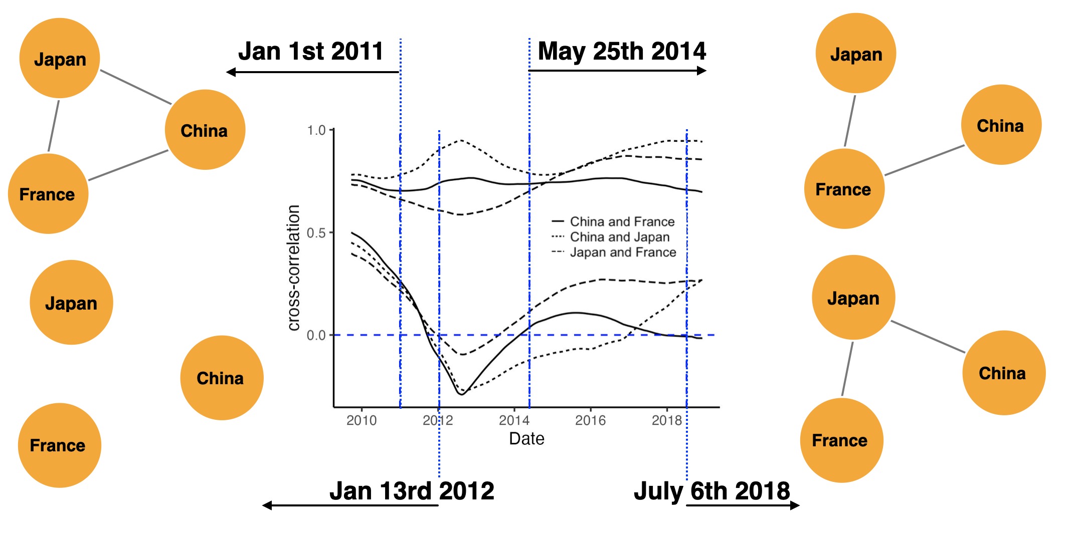
Figure 1.1: Middel panel: solid, dashed and dotted curves denote the SCBs of the cross-correlations of China and France, Japan and France, and China and Japan, respectively; Left and right panels: the snapshot of time-varying networks induced by $H_{0}=0$ on Jan 1st 2011, Jan 13rd 2012, May 25th 2014 and July 6th 2018, respectively.

In this paper, we establish a new framework for constructing time-varying correlation networks from non-stationary multivariate time series via multiple testing, largely addressing the drawbacks of correlation networks pointed out by Diebold and Yilmaz, (2014). Specifically, we build the time-varying correlation networks on a group of correlation-based similarity measures through a simultaneous test of the hypotheses for $(i,j,k)\in\mathbb{B}$, where $\mathbb{B}$ is a index subset of $\{(i,j,k):i,j=1,\cdots,p,k=0,\cdots,d_{n}\}$,

$$H_{0ijkt}:c_{ijk}(t)=g_{ijk}(t)\quad\text{versus}\quad H_{1ijkt}:c_{ijk}(t)\neq g_{ijk}(t),\quad t\in(0,1),$$ (1.1)

where $c_{ijk}(\cdot)$ is a time-rescaled (on $(0,1)$) correlation-based measure function between $(Y_{s,i})_{s=1}^{n-k}$ and $(Y_{s-k,j})_{s=k+1}^{n},$ $g_{ijk}(\cdot)$ is a pre-specified and possibly time-varying function. Simple and meaningful choices of $g_{ijk}(\cdot)$ include but are not limited to: (1) $g_{ijk}(\cdot)\equiv 0$ which tests for the presence of correlations; (2) $g_{ijk}(t)$ are constant functions for a given index set of $(i,j)$ to test for time-invariance of the corresponding sub-graph. Let $T(t)=(T_{ijk}(t))$ be the corresponding test statistics. We connect $i$ and $j$ at time $t$ if there exists some $k$ such that $T_{ijk}(t)\geq c_{1-\alpha}(t,i,j,k)$ where $c_{1-\alpha}(t,i,j,k)$ is the threshold that controls the family-wise error rate (FWER) of hypotheses in (1.1) at the nominal level $\alpha$. For brevity and without loss of generality, we consider $c_{ijk}(t)$ as time-varying and time-lagged cross-correlations of general time series $\mathbf{Y}_{t}:=f(\mathbf{Z}_{t},\cdots,\mathbf{Z}_{t-r})$ for $p_{1}$-dimensional non-stationary multivariate time series $\mathbf{Z}_{t}$, where $r$ is some fixed integer, and $f:(\mathbb{R}^{p_{1}})^{r}\rightarrow\mathbb{R}^{p}$ is a smooth vector function. Importantly, we alleviate the aforementioned limitation of the pairwise construction of correlation-based networks via the flexible choices of $f$. When $\mathbf{Y}_{t}=\mathbf{Z}_{t}$, our method is related to the linear Granger-causality test. When $\mathbf{Y}_{t}=((\mathbf{Z}_{t}\circ\mathbf{Z}_{t})^{\top},...,(\mathbf{Z}_{t}\circ\mathbf{Z}_{t-r})^{\top})^{\top}$, where $\circ$ stands for the Hadamard product, our method provides an alternative to Diebold and Yilmaz, (2014), gauging the connectedness in terms of volatility. Moreover, by considering high-order polynomials for $f$, we can measure high-order dependence in time series vectors even if the data is non-Gaussian, while the classic correlation can only capture pairwise linear dependence under Gaussianity and leads to the ‘linear, Gaussian thinking’ issue raised by Diebold and Yilmaz, (2014).

Our framework for recovering time-varying network structures is based on a new class of difference-based estimators and a novel bootstrap-assisted procedure, admitting flexible choices of $\mathbb{B}$ considered in (1.1). Our difference-based estimator circumvents the pre-estimation of complex trends and can be applied to general non-stationary linear or nonlinear processes (Zhou and Wu, (2010),Vogt, (2012), Dahlhaus et al., (2019), and Dette and Wu, (2022)) with piecewise smooth trends that allow for structure breaks commonly identified in many applications (see for instance Stărică and Granger, (2005), Bouri et al., (2019), and Karavias et al., (2022)). To tackle the functional constraints in (1.1) and control FWER, we provide a uniform bootstrap-assisted device for constructing simultaneous confidence bands (SCBs) for time-lagged cross-correlations of $(\mathbf{Y}_{t})$. The SCBs are defined by $\hat{U}_{\alpha,ijk}(\cdot)$ and $\hat{L}_{\alpha,ijk}(\cdot)$ estimated from data such that for $\alpha\in(0,1)$ as $n\to\infty$,

$$P(\hat{L}_{\alpha,ijk}(t/n)\leq\mathrm{corr}(Y_{t,i},Y_{t-k,j})\leq\hat{U}_{\alpha,ijk}(t/n),~{}1\leq t\leq n,(i,j,k)\in\mathbb{B})\to 1-\alpha,$$ (1.2)

where $Y_{t,i}$ is the $i_{th}$ component of $\mathbf{Y}_{t}$. By the dual property of hypothesis testing and confidence sets, we construct the time-varying network by connecting $i$ and $j$ at time $s\in(0,1)$ if $g_{ijk}(s)\not\in[\hat{L}_{\alpha,ijk}(s),\hat{U}_{\alpha,ijk}(s)]$. We present Figure 1.1 for illustration, where we infer dynamic networks from SCBs of the financial data ($S_{i}$ of Section 6). We display several sub-graphs of the induced network at different times that have distinct edge connections, demonstrating the changing dynamics. By controlling the FWER through SCBs, we are able to recover the time-varying network at all times with high probability, which is useful to investigate the evolving dynamics and transition of the interconnectedness of complex data. Finally, we develop an easily implementable variance reduction technique that uniformly reduces the widths of the equivalent SCBs (1.2) and increases the recovery probability that all the pairs of nodes are correctly linked. To the best of the authors’ knowledge, we are the first to consider the uniform variance reduction to obtain a smaller type II error rate of SCBs at a given significance level. In particular, we build the REduction-in-widths and Difference-based SCBs (RED-SCBs) applicable to high-dimensional time series data via a nonstandard wild bootstrap procedure. In the data analysis, equipped with the variance-reduced algorithm, we produce SCBs of cross-correlations contained fully in $[-1,1]$ when the original bands lie beyond this range. Theoretically, the uniform width reduction effect of RED-SCBs requires delicate analysis of the tail behavior of high dimensional Gaussian processes, which differentiates itself from its stationary univariate counterpart Cheng et al., (2007). Based on the results of Hüsler and Schüpbach, (1988) and Royen, (2014)(see also Latała and Matlak, (2017)), our argument provides a theoretical tool to evaluate tail probabilities for the maximum of multivariate and high dimensional Gaussian vectors with flexible covariance structures, which is of independent interest.

The rest of the paper is organized as follows. In Section 2, we present our main results on disclosing the time-varying network structure, including the estimation and inference procedures for the cross-correlation functions with many time-lags and a simple uniform variance reduction method. In Section 3, we establish a Gaussian approximation scheme for the estimated cross-correlation curves, the asymptotic FWER control of the proposed variance-reduced bootstrap-assisted algorithm, and the improvement of its overall recovery probability. We should point out that the asymptotic behavior of the maximum deviation of (auto)correlations over a fixed number of lags differs drastically from that over a diverging number of lags, making the simultaneous inference of (auto)correlations a long-standing difficult problem. We solve this problem as an important by-product. Section 4 gives the selection scheme of smoothing parameters. Section 5 reports the finite sample performance in simulation studies. In Section 6 we analyze the time-varying cross-correlation networks induced from Daily WRDS World indices. Section 7 provides conclusion remarks and discussions on future work. Appendix A presents detailed formulae for the estimators used in the RED-SCBs-based algorithm. In Appendix B we provide the detailed algorithm for time-varying cross-correlation analysis via difference-based SCBs and its theoretical properties. Appendix C offers auxiliary results and the proofs of theorems. The online supplement includes the algorithm of using plug-in estimators when the trends are smooth and the corresponding theoretical properties, as well as proofs of Theorem 3.1 and auxiliary results.

2 Main results

We first summarize the notation that will be used throughout the paper before stating our results formally. For a vector $\mathbf{v}=(v_{1},\cdots,v_{p})\in\mathbb{R}^{p}$, let $|\mathbf{v}|=(\sum_{j=1}^{p}v^{2}_{j})^{1/2}$. For a random vector $\mathbf{V}$, $q\geq 1$, let $\|\mathbf{V}\|_{q}=(\mathbb{E}|\mathbf{V}|^{q})^{1/q}$ denote the $\mathcal{L}_{q}$-norm of the random vector $\mathbf{V}$. Let $|\mathbf{z}|_{\infty}$ denote the maximum element of the vector $\mathbf{z}$. In this paper we consider the kernel function $K(\cdot)$ that is zero outside $(-1,1)$, and write $K_{\eta}=K(\cdot/\eta)$ for some bandwidth parameter $\eta$. For an index set $\mathbb{A}$, let $|\mathbb{A}|$ denote its cardinality. Let $\mathbf{1}(\cdot)$ denote the indicator function, and $\overset{p}{\to}$ denote convergence in probability.

We consider the time series model of the form : for $i=1,\cdots,p,~{}j=1,\cdots,n$,

$$Y_{j,i}=\mu_{i}(t_{j})+\epsilon_{j,i},\quad\mu_{i}(t)=\sum_{l=0}^{d_{i}}\mu_{i,l}(t)\mathbf{1}(a_{i,l}\leq t<a_{i,l+1}),$$ (2.1)

where $t_{j}=j/n$, $t\in[0,1]$, $(\epsilon_{j,i})_{j=1}^{n}$ is a locally stationary process(see Section 3 for the definition), $\mu_{i}(\cdot)$ is a deterministic function on $[0,1]$ with abrupt change points $0=a_{i,0}<a_{i,1}<\cdots<a_{i,d_{i}}<a_{i,d_{i}+1}=1$, $d_{i}$ is the number of change points, $\mu_{i,l}(t)$ is Lipschitz continuous over $[a_{i,l},a_{i,l+1}]$, and the Lipschitz constants of $\mu_{i,l}(\cdot)$ are uniformly bounded for $i=1,\cdots,p$, $0\leq l\leq d_{i}$. To construct the equivalent SCBs of (1.2), we start by introducing the definition of cross-correlation functions under time series non-stationarity. Define the $k_{th}$ $(k\in\mathbb{Z})$ order cross-covariance, cross-marginal variance and cross-correlation function as

$$\gamma_{k}^{i,l}(t)=\mathrm{Cov}(\epsilon_{\lfloor nt\rfloor,i},\epsilon_{\lfloor nt\rfloor+k,l}),\quad\sigma^{2}_{i,l}(t)=\gamma^{l,l}_{0}(t)\gamma^{i,i}_{0}(t),\quad\rho_{k}^{i,l}(t)=\gamma_{k}^{i,l}(t)/\sigma_{i,l}(t).$$ (2.2)

Notice that when $k\neq 0$, (2.2) indicates that in general $\rho^{i,l}_{k}(t)\neq\rho^{i,l}_{-k}(t)$ when $i\neq l$. In this case, the construction based on (1.1) will yield a directed network. In the rest of the paper, we will use a single index $s$ to stand for the double indices $i,l$ of the superscript when $i=l=s$ if no confusion is caused.

Remark 2.1.

If it’s known that there are no change points, i.e., $d_{i}=0$, $1\leq i\leq p$, one can estimate the correlation functions in (2.2) via the non-parametric residual $\hat{\epsilon}_{j,i}=Y_{j,i}-\hat{\mu}_{i}(t_{j})$, where $\hat{\mu}_{i}(\cdot)$ is the local linear estimator of $\mu_{i}(\cdot)$, see Zhou and Wu, (2010) and Appendix D of the online supplement where we provide algorithms for constructing correlation networks based on $\hat{\epsilon}_{j,i}$. In the main article, we shall focus on the $d_{i}>0$ case and propose difference-based estimators, as in the subsequent sections.

2.1 Difference-based sample correlation curves

When $(\mathbf{Y}_{t})_{t=1}^{n}$ is contaminated by unknown abrupt change points, the direct estimation of their piecewise smooth trends will be sophisticated. In fact, there have been no methods designed for this problem. A related problem is to consistently identify a (diverging) number of abrupt change points from the piecewise smooth mean of general non-stationary time series, which has been only considered recently by Wu and Zhou, (2019). Therefore, a straightforward approach to remove piecewise smooth trends is to separately apply the local linear estimation to the subseries between the identified jump points. However, this will cause severe boundary issues in practice, which are well-known in the field of kernel estimation, see for example Cheng et al., (1997).

Alternatively, we propose a difference-based approach for (2.2), which has succeeded in estimating variance (see Müller and Stadtmuller, (1987) and Hall et al., (1990)), long-run variance (see Dette and Wu, (2019)), and autocovariance (see Inder and Axel, (2017) and Cui et al., (2021)) without the pre-estimation of the trend function. Define $\tilde{\epsilon}^{i}_{j,k}=\epsilon_{j,i}-\epsilon_{j-k,i}$. Let $\beta^{i,l}_{k}(t_{j}):=\mathbb{E}(\tilde{\epsilon}^{i}_{j+k,k}\tilde{\epsilon}^{l}_{j+k,h})$ for some large $h=o(n)$. Then under the locally stationary 3.1 stated in Section 3, $\beta^{i,l}_{k}(\cdot)$ is a smooth function on $[0,1]$. Notice that by 3.1 we can select a positive $\tilde{h}<h$ such that $\gamma^{i,l}_{k}(t)\approx 0$ for $|k|\geq\tilde{h}$. Note that for $k\leq h-\tilde{h}$,

$$\beta^{i,l}_{k}(t_{j}) =E(\epsilon_{j+k,i}-\epsilon_{j,i})(\epsilon_{j+k,l}-\epsilon_{j+k-h,l})$$ (2.3)

$$=\gamma^{i,l}_{0}(t_{j+k})+\gamma^{i,l}_{k-h}(t_{j})-\gamma^{i,l}_{-h}(t_{j+k})-\gamma^{i,l}_{k}(t_{j})\approx\gamma^{i,l}_{0}(t_{j})-\gamma^{i,l}_{k}(t_{j}).$$ (2.4)

Further define $\tilde{y}^{i}_{j,k}=Y_{j,i}-Y_{j-k,i}$, $\tilde{\mu}^{i}_{j,k}=\mu_{i}(t_{j})-\mu_{i}(t_{j-k})$, and hence $\tilde{y}_{j,k}^{i}=\tilde{\mu}_{j,k}^{i}+\tilde{\epsilon}_{j,k}^{i}$. By the piecewise smoothness of $\mu_{i}(\cdot)$, $1\leq i\leq p$, under some mild conditions it follows that

$$\sum_{j=1}^{n}K_{b}(t_{j}-t)\tilde{y}^{i}_{j,k}\tilde{y}^{l}_{j,h} =\sum_{j=1}^{n}K_{b}(t_{j}-t)(\tilde{\epsilon}^{i}_{j,k}\tilde{\epsilon}^{l}_{j,h}+\tilde{\mu}^{i}_{j,k}\tilde{\mu}^{l}_{j,h}+\tilde{\epsilon}^{i}_{j,k}\tilde{\mu}^{l}_{j,h}+\tilde{\epsilon}^{l}_{j,h}\tilde{\mu}^{i}_{j,k})$$ (2.5)

$$\approx\sum_{j=1}^{n}K_{b}(t_{j}-t)\tilde{\epsilon}^{i}_{j,k}\tilde{\epsilon}^{l}_{j,h},$$ (2.6)

see the proof of Lemma 1 of the supplement for details. Hence, by the continuity of $\beta_{k}^{i,l}(\cdot)$, we have

$$\sum_{j=1}^{n}K_{b}(t_{j}-t)E\big{(}\tilde{y}^{i}_{j,k}\tilde{y}^{l}_{j,h}\big{)}\approx\sum_{j=1}^{n}K_{b}(t_{j}-t)\beta^{i,l}_{k}(t_{j-k})\approx\gamma^{i,l}_{0}(t)-\gamma_{k}^{i,l}(t).$$ (2.7)

Therefore, we can consistently estimate $\gamma_{0}^{i,l}(t)-\gamma_{k}^{i,l}(t)$ by the local linear estimator $\hat{\beta}_{k}^{i,l}(t)$ such that

$$(\hat{\beta}_{k}^{i,l}(t),\hat{\beta}_{k}^{i,l,\prime}(t))^{\top}=\underset{(\eta_{0},\eta_{1})\in\mathbb{R}^{2}}{\mathrm{argmin}}\sum_{j=1}^{n}\left(\tilde{y}^{i}_{j,k}\tilde{y}^{l}_{j,h}-\eta_{0}-\eta_{1}(t_{j}-t)\right)^{2}K_{b^{i,l}_{k}}(t_{j}-t),$$ (2.8)

where $b^{i,l}_{k}$ is the bandwidth parameter. Define the centered version of $\tilde{\epsilon}^{i}_{j,k}\tilde{\epsilon}^{l}_{j,h}$ as

$$\tilde{e}^{i,l}_{j,k}:=\tilde{\epsilon}^{i}_{j,k}\tilde{\epsilon}^{l}_{j,h}-\beta^{i,l}_{k}(t_{j-k}),$$ (2.9)

with $\tilde{e}^{i,l}_{j,0}=0$ since $\tilde{\epsilon}^{i}_{j,0}=0$ by definition. For $(i,l,k)\in\mathbb{B}$, since $\tilde{\epsilon}^{i}_{j,k}\tilde{\epsilon}^{l}_{j,h}$ is the product of the differences of locally stationary processes, $\tilde{e}^{i,l}_{j,k}$ is also locally stationary (see definitions in Section 3). Under mild conditions, by stochastic expansion (see Corollary F.1 of the supplement for details), we have

$$\max_{(i,l,k)\in\mathbb{B}}\sup_{t\in\mathcal{T}}\left|\hat{\beta}^{i,l}_{k}(t)-\beta^{i,l}_{k}(t)-\frac{1}{nb_{k}^{i,l}}\sum_{j=1}^{n}K_{b^{i,l}_{k}}(t_{j}-t)\tilde{e}^{i,l}_{j,k}\right|=o_{\mathbb{P}}(1),$$ (2.10)

where $\mathbb{B}$ is as defined in (1.1). Analogous to (2.8) and using (2.4), the local linear estimator $\hat{\beta}_{h}^{i,l}(t)$ is a consistent estimator of $2\gamma_{0}^{i,l}(t)$. As a consequence, the cross-covariance function $\gamma^{i,l}_{k}(t)$ can be estimated by $\tilde{\gamma}^{i,l}_{k}(t)=\hat{\beta}^{i,l}_{h}(t)/2-\hat{\beta}^{i,l}_{k}(t)$ and the cross-correlation function $\rho_{k}^{i,l}(t)$ can be estimated by

$$\tilde{\rho}^{i,l}_{k}(t)=\tilde{\gamma}^{i,l}_{k}(t)/\tilde{\sigma}_{i,l}(t),\quad\tilde{\sigma}_{i,l}(t)=\sqrt{\tilde{\gamma}^{i}_{0}(t)\tilde{\gamma}^{l}_{0}(t)}.$$ (2.11)

For simplicity, let $z$ denote the triad $(i,l,k)$, and we use $b_{z}$, $\rho_{z}(t)$, $\sigma_{z}(t)$ to denote $b^{i,l}_{k}$, $\rho^{i,l}_{k}(t)$, $\sigma_{i,l}(t)$.

2.2 Variance reduction

Albeit by definition the correlation function lies inside $[-1,1]$, in practice the nonparametric confidence band of the correlation curve could exceed $[-1,1]$ (see for instance Figure 5 in Zhao, (2015)) and becomes less informative and less sensitive, especially for the inference of connections. To enhance the probability of recovering true connections, we develop a uniform variance reduction technique by interpolating at selected points to further narrow the SCBs without changing the nominal level. The improved SCBs (i.e., RED-SCBs) admit simple forms with only a slight computational cost and project effectively the corresponding asymptotic reduction effect into finite samples. Our inspiration comes from the literature on variance reduction for $i.i.d.$ errors and pointwise inference (see for example Efron, (1990) and Cheng et al., (2007)). However, their dependent and non-stationary counterparts remain largely untouched, let alone the extension of their pointwise reduction effects for fixed $t\in[0,1]$ to the uniform reduction effect on $(0,1)$.

Specifically, we propose to use the following linear combination of $\hat{\beta}_{z}(t)$ to refine the estimate of $\beta_{z}(t)$,

$$\check{\beta}_{z}(t)=\{\check{\beta}_{z,+}(t)+\check{\beta}_{z,-}(t)\}/2,\quad\check{\beta}_{z,\pm}(t)=\sum_{j=0,1,2}A_{j}(\pm r)\hat{\beta}_{z}(t-(\pm r+1-j)\omega_{z}(t)),$$

where $A_{0}(r)=r(r-1)/2,A_{1}(r)=\left(1-r^{2}\right),A_{2}(r)=r(r+1)/2$, for some selected $r\in(-1,1)$, and $\omega_{z}(t)=\delta(t)b_{z}$, $\delta(t)=\min\{\delta,(t-b)/[(r+1)b],(1-b-t)/[(r+1)b]\}$ where $\delta$ is a non-negative constant. The above estimate utilizes the correlation between $\hat{\beta}_{z}(t_{1})$ and $\hat{\beta}_{z}(t_{2})$ when $t_{1},t_{2}$ fall into the vicinity of $t$ to achieve smaller variance, while the coefficients $A_{i}(r)$, $i=1,2,3$ are carefully designed such that the asymptotic bias is not changed. In the formula of $\check{\beta}_{z}(\cdot)$, $\omega_{z}(t)$ controls the range of the smoothing neighborhood through $\delta$ and $b_{z}$. In particular, when $\delta=0$, $\check{\beta}_{z}(t)$ equals the original estimator $\hat{\beta}_{z}(t)$ and the variance remains unchanged. In practice, a large $\delta$ is superior when the trend function is smooth and the noise level is low, while a smaller $\delta$ is preferred when the signals contain many abrupt change points. Our final variance-reduced estimators of cross-correlations are

$$\check{\rho}_{z}(t)=\check{\gamma}_{z}(t)/\check{\sigma}_{z}(t),\quad\check{\sigma}_{z}(t)=\sqrt{\check{\gamma}^{i}_{0}(t)\check{\gamma}^{l}_{0}(t)},\quad z=(i,l,k)\in\mathbb{B},$$ (2.12)

where $\check{\gamma}_{z}(t)=\check{\beta}^{i,l}_{h}(t)/2-\check{\beta}^{i,l}_{k}(t)$ and $\check{\gamma}^{l}_{0}(t)=\check{\beta}^{l}_{h}(t)/2.$

2.3 Controlling FWER via bootstrap-assisted inference

To motivate our bootstrap algorithm for the inference of time-varying networks, notice that the key to valid SCBs of (1.2) is the quantiles of

$$\max_{z\in\mathbb{B}}\sup_{t\in[b,1-b]}\sqrt{nb_{z}}|\check{\rho}_{z}(t)-\rho_{z}(t)|,$$ (2.13)

where $b_{z}$ is the bandwidth parameter and $b=b_{n}:=\max_{z\in\mathbb{B}}b_{z}$ converges to $0$ as $n\to\infty$, so that $\cup_{n}[b_{n},1-b_{n}]=(0,1)$. In addition to the time-varying data-generating mechanism, we allow $p$ and $d_{n}$ to be either fixed or divergent for the index set $\mathbb{B}$. We shall begin with deriving the SCBs of

$$\max_{z\in\mathbb{B}}\sup_{t\in[b,1-b]}\sqrt{nb_{z}}|\tilde{\rho}_{z}(t)-\rho_{z}(t)|,$$ (2.14)

and show how the result of (2.14) can lead to the solution of (2.13).

The distributional properties of (2.14) have been only partially theoretically investigated in time series analysis of autocorrelations (i.e., $p=1$). For example, Zhao, (2015) tackles the case when $p=d_{n}=1$, i.e., the simultaneous inference of the local correlation curve. Xiao and Wu, (2014) and Braumann et al., (2021) consider $p=1$ under the assumption of stationarity, where $\rho_{k}(t)=\rho_{k}$. Specifically, the theoretical conclusions of Xiao and Wu, (2014) necessitate that $d_{n}$ diverges, while the asymptotic results of Braumann et al., (2021) allow for finite $d_{n}$ but require the underlying time series to be linear. Due to the sophisticated distributional properties and to achieve better finite sample performance, Xiao and Wu, (2014) proposes blocks of block bootstrap and Braumann et al., (2021) develops AR-sieve-based bootstrap for the linear process. However, their method cannot be applied to the inference of time-varying correlation networks, mainly because those methods are designed for stationary processes of which the correlation curves are constants.

We start by investigating the stochastic expansion of the cross-correlation estimate. Following (2.10) and (2.11), we could approximate the maximum deviation of the cross-correlation estimate via $\vartheta_{z}(t)$, the moving weighted average of innovations, i.e.,

$$\max_{z\in\mathbb{B}}\sup_{t\in[b,1-b]}\sqrt{nb_{z}}\left|\tilde{\rho}_{z}(t)-\rho_{z}(t)-\vartheta_{z}(t)\right|=o_{\mathbb{P}}(1),$$ (2.15)

where $\vartheta_{z}(t)=(nb_{z})^{-1}\sum_{j=1}^{n}K_{b_{z}}(t_{j}-t)\Xi_{z,j}$, and

$$\Xi_{z,j} :=(\tilde{e}^{i,l}_{j,h}/2-\tilde{e}^{i,l}_{j,k})/\sigma_{i,l}(t_{j})-4^{-1}\rho^{i,l}_{k}(t_{j})\left(\tilde{e}^{i}_{j,h}/\gamma^{i}_{0}(t_{j})+\tilde{e}^{l}_{j,h}/\gamma^{l}_{0}(t_{j})\right).$$ (2.16)

When $i=l$, $\Xi_{z,j}$ reduces to $\sigma^{-1}_{i}(t_{j})(\tilde{e}^{i}_{j,h}/2-\tilde{e}^{i}_{j,k}-\rho^{i}_{k}(t_{j})\tilde{e}^{i}_{j,h}/2)$, which is the stochastic error of the difference-based counterpart of (A.8) in Zhao, (2015), where the data is required to be zero-mean. The first term of (2.16) is due to the approximation to $(\tilde{\gamma}_{z}(t)-\gamma_{z}(t))/\sigma_{z}(t)$, while the second term of (2.16) mainly accounts for the approximation error of $(\tilde{\sigma}_{z}(t)-\sigma_{z}(t))/\tilde{\sigma}_{z}(t)$.

As a result of (2.14) and (2.15), we can obtain SCBs and infer the time-varying network structures through the quantiles of $\max_{z\in\mathbb{B}}\sup_{t\in[b,1-b]}\sqrt{nb_{z}}|\vartheta_{z}(t)|$, where $\mathbb{B}$ is defined in (1.1). Let $c_{z}=(b/b_{z})^{1/2}$, where $b=\max_{z\in\mathbb{B}}b_{z}$, and $\tilde{\Gamma}^{2}_{z}(t)$ be the limiting variance of $\sqrt{nb_{z}}|\vartheta_{z}(t)|$, of which the existence and non-degeneracy are ensured by Lemma C.3 of Dette and Wu, (2021) and 3.4. Furthermore, we can construct time-varying networks with time-varying and edge-specific thresholds of (1.1) via estimating $\tilde{\Gamma}_{z}(t)$ and deriving the quantiles of $\max_{z\in\mathbb{B}}\sup_{t\in[b,1-b]}\sqrt{nb_{z}}|\vartheta_{z}(t)|/\tilde{\Gamma}_{z}(t)$, which can be approximated by the maximum of a possibly high dimensional vector. To this end, we concatenate the related random variables adjusted by variances and bandwidths in a block of dimension $|\mathbb{B}|$ :

$$\bar{\mathbf{\Xi}}_{j,s}^{\mathbb{B}}:=(c_{z}K_{b_{z}}(t_{j}-t_{s})\Xi_{z,j}/\tilde{\Gamma}_{z}(t_{s}),z\in\mathbb{B})^{\top},\quad 1\leq j,s\leq n,~{}t_{s}=s/n.$$ (2.17)

Under mild conditions, we have $\underset{1\leq s\leq n}{\max}\left|\sum_{j=1}^{n}\bar{\mathbf{\Xi}}_{j,s}^{\mathbb{B}}/\sqrt{nb}\right|_{\infty}\approx\underset{z\in\mathbb{B}}{\max}\underset{t\in[b,1-b]}{\sup}\sqrt{nb_{z}}|\vartheta_{z}(t)|/\tilde{\Gamma}_{z}(t)$, see the proof of Theorem 3.1 in the supplement for details. The popular method to mimic the distributional properties of $\underset{1\leq s\leq n}{\max}\left|\sum_{j=1}^{n}\bar{\mathbf{\Xi}}_{j,s}^{\mathbb{B}}/\sqrt{nb}\right|_{\infty}$ is the multiplier bootstrap using the block sums of time series vector $(\mathbf{\bar{\Xi}}^{\mathbb{B},\top}_{j,1},\cdots,\mathbf{\bar{\Xi}}^{\mathbb{B},\top}_{j,n})^{\top}_{1\leq j\leq n}$, see Zhang and Cheng, (2018). However, such an approach will be inconsistent due to the sparsity of $\mathbf{\bar{\Xi}}^{\mathbb{B}}_{j,s}$ caused by the bounded support of kernel $K(\cdot)$, see the discussion in Section 2.1 of Dette and Wu, (2021). To address this issue, we compress the aforementioned sparse vector series, rearrange the blocks and obtain the following $(n-2\lceil nb\rceil+1)|\mathbb{B}|$ dimensional vectors

$$\bar{\mathbf{\Xi}}_{j}^{\mathbb{B}}=(\bar{\mathbf{\Xi}}_{j,\lceil nb\rceil}^{\mathbb{B},\top},\bar{\mathbf{\Xi}}_{j+1,\lceil nb\rceil+1}^{\mathbb{B},\top},\cdots,\bar{\mathbf{\Xi}}_{n-2\lceil nb\rceil+j,n-\lceil nb\rceil}^{\mathbb{B},\top})^{\top},1\leq j\leq 2\lceil nb\rceil,$$ (2.18)

such that $\left|\sum_{j=1}^{2\lceil nb\rceil}\bar{\mathbf{\Xi}}_{j}^{\mathbb{B}}/\sqrt{nb}\right|_{\infty}=\underset{1\leq s\leq n}{\max}\left|\sum_{j=1}^{n}\bar{\mathbf{\Xi}}_{j,s}^{\mathbb{B}}/\sqrt{nb}\right|_{\infty}$. In fact, $\bar{\mathbf{\Xi}}_{j}^{\mathbb{B}}$ in (2.18) extends the vector $\hat{\tilde{Z}}^{\hat{\sigma}}_{j}$ in Equation (2.26) of Dette and Wu, (2021) to multivariate non-stationary second-order processes allowing various bandwidths, which enables us to develop a “non-standard block wild bootstrap” which recovers the desired correlation networks based on (1.1) while controlling the family-wise type I error regardless of the divergence of the cardinality of the index set $\mathbb{B}$ or the presence of nonlinearity and non-stationarity in the time series. The detailed algorithm is deferred to Algorithm 1 in Appendix B.

Note that the linear combination of $\hat{\beta}_{z}(t)$ at nearby points is asymptotically equivalent to the local linear estimator of $\beta_{z}(\cdot)$ using the high-order kernel $\check{K}(\cdot)$, where $\check{K}(t)=(\check{K}_{+}(t)+\check{K}_{-}(t))/2$, and $\check{K}_{\pm}(t)=\sum_{j=0,1,2}A_{j}(\pm r)K(t+(\pm r+1-j)\delta)$. Therefore, the bootstrap procedure based on the high-dimensional vector (2.18) can be easily adapted to (2.13) via changing the kernel function $K(\cdot)$ by $\check{K}(\cdot)$ in $\vartheta_{z}(t)$, $\tilde{\Gamma}_{z}(t)$ and $\bar{\boldsymbol{\Xi}}^{\mathbb{B}}_{j,s}$, which are denoted by $\check{\vartheta}_{z}(t)$, $\check{\Gamma}_{z}(t)$ and $\check{\boldsymbol{\Xi}}^{\mathbb{B}}_{j,s}$. We can define the variance-reduced estimators $\hat{\check{\mathbf{\Xi}}}_{i}^{\mathbb{B}}$ and $\hat{\check{\Gamma}}_{z}^{2}(t)$ as the estimators of ${\check{\mathbf{\Xi}}}_{i}^{\mathbb{B}}$ and ${\check{\Gamma}}_{z}^{2}(t)$, see Appendix A for detailed formulae. In Algorithm 1, we provide the full algorithm.

Algorithm 1 Time-varying cross-correlation analysis via RED-SCBs

1:Compute $\check{\rho}^{i,l}_{k}(t)$, $(i,l,k)\in\mathbb{B}$ defined in (2.12).

2:Compute the $|\mathbb{B}|$-dimensional vectors $\hat{\check{\mathbf{\Xi}}}_{j,s}^{\mathbb{B}}$ using (A.3), $1\leq j,s\leq n$.

3:For a window size $w$, compute $\hat{\check{\mathbf{S}}}_{l,j}^{\mathbb{B}}=\sum_{s=j-w+1}^{j}\hat{\check{\mathbf{\Xi}}}_{s+l,\lceil nb\rceil+l}^{\mathbb{B}}-\sum_{s=j+1}^{j+w}\hat{\check{\mathbf{\Xi}}}_{s+l,\lceil nb\rceil+l}^{\mathbb{B}}$, where $l=0,\cdots,n-2\lceil nb\rceil$.

4:for $r=1,\cdots,B$ do

5:     Generate independent standard normal random variables $R_{j}^{(r)}$, $j=1,\cdots,n$.

6:     Recall that $b=\max_{(i,l,k)\in\mathbb{B}}b^{i,l}_{k}$. Calculate

$$\check{Z}_{\mathrm{boot}}^{(r)}=\frac{\underset{0\leq l\leq n-2\lceil nb\rceil}{\max}\left|\sum_{j=w}^{2\lceil nb\rceil-w}\hat{\check{\mathbf{S}}}_{l,j}^{\mathbb{B}}R^{(r)}_{l+j}\right|_{\infty}}{\sqrt{2w\lceil nb\rceil}}.$$

7:end for

8:Let $\check{r}_{\mathrm{boot}}$ denote the $(1-\alpha)$-quantile of the bootstrap sample $\check{Z}_{\mathrm{boot}}^{(1)},\cdots,\check{Z}_{\mathrm{boot}}^{(B)}$.

9:Connect $i$ and $l$ at time $t\in[b,1-b]$ if $|g_{ilk}(t)-\check{\rho}^{i,l}_{k}(t)|>\check{r}_{\mathrm{boot}}(nb^{i,l}_{k})^{-1/2}\hat{\check{\Gamma}}^{i,l}_{k}(t)$ for some $k$ such that $(i,l,k)\in\mathbb{B}$.

Algorithm 1 is different from the conventional block bootstrap (Lahiri, (2003)) in two aspects. First, most conventional block bootstrap methods are aimed at imitating the original time series and deriving the limiting distribution of a statistic (see for instance Section 2.5 of Lahiri, (2003)), while Algorithm 1 approximates the maximum of the multivariate or possibly high-dimensional estimation errors. Therefore, it produces asymptotically correct tests for (1.1) even though the distribution of (2.13) under finite $|\mathbb{B}|$ differs drastically from that under diverging $|\mathbb{B}|$. Second, the summands $\hat{\check{\mathbf{S}}}_{l_{1},j_{1}}^{\mathbb{B}}$ and $\hat{\check{\mathbf{S}}}_{l_{2},j_{2}}^{\mathbb{B}}$ share the same Gaussian multipliers if $l_{1}+j_{1}=l_{2}+j_{2}$, which contrasts with the classic procedures where the summands are multiplied by independent Gaussian variables, see for example Theorem 5 of Zhou, (2013). Furthermore, Algorithm 1 is suitable for efficient parallel computing. In Algorithm 1 we can compute $\left|\sum_{j=w}^{2\lceil nb\rceil-w}\hat{\check{\mathbf{S}}}_{l,j}^{\mathbb{B}}R^{(r)}_{l+j}\right|_{\infty}$ for separate blocks of $l$ and combine their maximums to obtain $\check{r}_{\mathrm{boot}}$, based on which we can further infer time-varying networks.

Remark 2.2.

To incorporate the prior knowledge of the network connections into our quantitative analysis, it is important to allow for flexible choices of $\mathbb{B}$. In Section 3 we show that Algorithm 1 is consistent under very mild conditions on $\mathbb{B}$. In particular, $|\mathbb{B}|$ can be either fixed or diverging depending on the practical interest. To the best of our knowledge, there are no existing justified methods for inferring correlations that are valid for general time series under both scenarios of a fixed number of lags and a diverging number of lags.

Remark 2.3.

Inference of correlation networks and testing of correlation matrices have been investigated by Efron, (2007), Cai and Liu, (2016), and Bailey et al., (2019), where they focus on static networks and require independence over time. Recently, time-varying or dynamic networks inferred from time series are increasingly studied, see Basu and Rao, (2021) and Chen et al., (2022). The newly proposed methods therein construct one uniform network structure from time series with changing data generating mechanisms. However, those methods cannot be directly used to infer infinite-dimensional time-varying network structures caused by the complex dynamic structure and generating mechanism of the system. In contrast, through controlling the FWER, the proposed Algorithm 1 recovers time-varying networks at all time points with high probabilities, see the next section for theoretical guarantee.

3 Theoretical properties

In this section, we shall examine the theoretical performance of Algorithm 1 in the aspects of type I error and recovery probability, while the theoretical properties of Algorithm 1 can be found in Appendix B. To state the theoretical results rigorously, we introduce the following notation and assumptions. Assume the processes $(\epsilon_{i,j})_{i=1}^{n}$ in (2.1) and $(\tilde{e}_{z,j})_{j=1}^{n}$ ($\tilde{e}^{i,l}_{j,k}$ in (2.9)) admit

$$\epsilon_{j,i}=G_{i}(t_{j},\mathcal{F}_{j}),\quad\tilde{e}_{z,j}=H_{z}(t_{j},\mathcal{F}_{j}),\quad 1\leq j\leq n,~{}1\leq i\leq p,~{}z=(i,l,k)\in\mathbb{B},$$

where $G_{i}(\cdot,\cdot)$ and $H_{z}(\cdot,\cdot)$ are measurable functions of $[0,1]\times\mathbb{R}^{\mathbb{Z}}\rightarrow\mathbb{R}$, $\mathcal{F}_{j}=(\boldsymbol{\xi}_{-\infty},...,\boldsymbol{\xi}_{j})$ is a filtration and $(\boldsymbol{\xi}_{i})_{i\in\mathbb{Z}}$ are $i.i.d.$ random elements. Define $\tilde{\mathbb{B}}(t)=\{z\in\mathbb{B}:\rho_{z}(t)\neq g_{z}(t)\}$, $t\in[0,1]$. For a set $A$, let $\bar{A}$ denote its complement. For $t\in[0,1]$, write $\sqrt{nb_{z}}|g_{z}(t)-\check{\rho}_{z}(t)|/\hat{\check{\Gamma}}_{z}(t)$ as $\check{T}_{z}(t)$ and let $\check{N}(t)=\{\check{T}_{z}(t)\leq\check{r}_{\mathrm{boot}},z\in\mathbb{B}\cap\bar{\tilde{\mathbb{B}}}(t)\}\cap\{\check{T}_{z}(t)>\check{r}_{\mathrm{boot}},z\in\tilde{\mathbb{B}}(t)\}$. The FWER (conditional on data) is

$$1-P_{H_{0}}(\{\check{T}_{z}(t)\leq\check{r}_{\mathrm{boot}},z=(i,l,k)\in\mathbb{B},t\in[b,1-b]\}|\mathcal{F}_{n}),$$

where $H_{0}$ denotes the null hypotheses of (1.1). The recovery probability of time-varying networks conditional on data based on RED-SCBs can be expressed as

$$\quad\int_{0}^{1}P(\check{N}(t)|\mathcal{F}_{n})dt.$$ (3.1)

We shall show that Algorithm 1 can control the FWER and enjoys the property of recovering the time-varying network structure with probability at least $1-\mathrm{FWER}$ in the subsequent analysis via SCBs.

The crucial ingredient of our Algorithm 1 is to mimic directly the maximum deviation of the estimated correlation curves instead of its limiting distribution since the limiting behavior of the maximum deviation of the difference-based non-parametric estimators for non-stationary nonlinear multivariate time series (2.1) rests on $\mathbb{B}$ in a complicated way. To see this, consider univariate stationary time series $X_{1}$,…,$X_{n}$, with autocorrelations $\rho(k)$ and their sample version $\hat{\rho}(k)=\hat{\gamma}(k)/\hat{\gamma}(0)$ where $\hat{\gamma}(k)=\frac{1}{n}\sum_{i=1}^{n-h}X_{i}X_{i+k}$. The asymptotic distribution of $\sqrt{n}\max_{1\leq k\leq d_{n}}|\hat{\rho}(k)-\rho(k)|$ for fixed $d_{n}$ depends on the fourth order structure of the time series, while for diverging $d_{n}$ the asymptotic distribution is Gumbel-type and solely rests on the second-order properties, provided that $E(|X_{i}|^{q})<\infty$ for $q>4$, see the discussion in Braumann et al., (2021). We avoid the difficulties caused by complicated limiting distributions by approximating the maximum deviation of the estimate via the Gaussian approximation and comparison techniques for sparse and high dimensional time series established by Dette and Wu, (2021), and show that Algorithm 1 yields valid tests adaptive to the size of $|\mathbb{B}|$.

For a process $L(t,\mathcal{F}_{i})$, we say it is $\mathcal{L}^{q}$ stochastic Lipschitz continuous (denoted by $L(\cdot,\cdot)\in\mathrm{Lip}_{q}$) if for $t_{1},t_{2}\in[0,1]$, there exists a constant $C>0$ such that

$$\|L(t_{1},\mathcal{F}_{0})-L(t_{2},\mathcal{F}_{0})\|_{q}\leq C|t_{1}-t_{2}|.$$ (3.2)

If $q\geq 2$, then the process $L(t,\mathcal{F}_{j})$ is locally stationary (LS). The LS process models the complex and smooth temporal dynamics of the error processes in (2.1). Our definition of the LS process is based on the Bernoulli shift process, which provides a fundamental framework for modeling nonlinear non-stationary processes, see Dahlhaus et al., (2019) for a comprehensive review. Let $\mathcal{F}^{*}_{j}=(\mathcal{F}_{-1},\boldsymbol{\varepsilon}^{\prime}_{0},\boldsymbol{\varepsilon}_{1},\cdots,\boldsymbol{\varepsilon}_{j-1},\boldsymbol{\varepsilon}_{j})$ where $\boldsymbol{\varepsilon}_{0}^{\prime}$ is an $i.i.d.$ copy of $\boldsymbol{\varepsilon}_{0}$. The physical dependence measure of the nonlinear filter $L(\cdot,\cdot)\in\mathrm{Lip}_{q}$ ($q>0$) is defined by $\delta_{q}(L,k)=\underset{t\in[0,1]}{\sup}\|L(t,\mathcal{F}_{k})-L(t,\mathcal{F}_{k}^{*})\|_{q}$, which quantifies the influence of the input $\boldsymbol{\varepsilon}_{0}$ on the output $L(\cdot,\mathcal{F}_{k})$. Finally, for a univariate LS time series $L(t,\mathcal{F}_{j})$, its long-run variance function is defined as

$$\sigma^{2}(L,t)=\sum_{k\in\mathbb{Z}}\mathrm{Cov}(L(t,\mathcal{F}_{0}),L(t,\mathcal{F}_{k})),~{}t\in[0,1].$$

Assumption 3.1.

For some $q\geq 4$, the error process $\epsilon_{j,i}=G_{i}(t_{j},\mathcal{F}_{j})$ satisfies,

1. $G_{i}(\cdot,\cdot)\in\mathrm{Lip}_{2q}$, $i=1,2,\cdots,p$ and their Lipschitz constants are uniformly bounded.

2. There exists a positive constant $t_{0}$ such that $\underset{t\in[0,1],i=1,2,\cdots,p}{\sup}\mathbb{E}(t_{0}\exp(G_{i}(t,\mathcal{F}_{0})))<\infty$.

3. $\max_{i=1,\cdots,p}\delta_{2q}(G_{i},l)=O(\chi^{l})$, for some $\chi\in(0,1)$ .

4. The second derivative $\gamma_{z}^{\prime\prime}(\cdot)$ of the function $\gamma_{z}(\cdot)$ exists and is Lipschitz continuous on $[0,1]$. The Lipschitz constants are bounded for all $z\in\mathbb{B}$.

The conditions (A1), (A3) and (A4) in 3.1 are standard in the kernel-based nonparametric analysis of LS time series. Similar assumptions have been posited by Zhao, (2015) for the inference of the univariate autocorrelation functions. 3.1 is mild in the sense of admitting time series with sub-exponential tails.

Assumption 3.2.

The kernel $K(\cdot)$ is a symmetric function which is zero outside $(-1,1)$ such that $\int_{-\infty}^{\infty}K(u)du=1$, $\int_{-\infty}^{\infty}u^{2}K(u)du=0$, $\int_{-\infty}^{\infty}(K^{\prime}(u))^{2}du<\infty$, and the second order derivative $K^{\prime\prime}$ is Lipschitz continuous on $(0,1)$.

It can be verified that if $K(\cdot)$ satisfies 3.2, so does $\check{K}(\cdot)$ which is the equivalent kernel for the variance-reduced correlation curve estimator $\check{\rho}(\cdot)$.

Assumption 3.3.

There exists a constant $c^{*}>0$ such that $\min_{z\in\mathbb{B}}b_{z}/b\geq c^{*}$.

3.3 imposes that all $(b_{z})_{z\in\mathbb{B}}$ share the same magnitude of orders.

Assumption 3.4.

The following assumptions hold for $\tilde{\Gamma}_{z}(\cdot)$ and change points:

1. The limiting variance function $\tilde{\Gamma}^{2}_{z}(t):=\lim_{n\to\infty}\mathrm{Var}(\sqrt{nb_{z}}\vartheta_{z}(t))$ ($\vartheta_{z}(t)$ is defined in (2.16)) is finite and well defined for $t\in[0,1]$, and that $\min_{z\in\mathbb{B}}\inf_{t\in[0,1]}\tilde{\Gamma}^{2}_{z}(t)>0$.

2. $\max_{z\in\mathbb{B}}\sup_{t\in(0,1)}|\tilde{\Gamma}_{z}^{\prime}(t)|<\infty$, where $\tilde{\Gamma}_{z}^{\prime}(t)$ is the derivative of $\tilde{\Gamma}_{z}(t)$.

3. The number of abrupt change points $d:=\max_{1\leq i\leq p}d_{i}=O(n^{\phi})$, $0\leq\phi<2/5$, and for a sufficiently large constant $D$, $\underset{1\leq i\leq p}{\max}\underset{1\leq l\leq d_{i}}{\max}|\mu_{i,l}(a_{i,l}^{+})-\mu_{i,l}(a_{i,l}^{-})|\leq D<\infty$.

Condition (B1) guarantees that $\tilde{\Gamma}^{2}_{z}(t)$ is non-degenerate. By the Lemma C.3 of Dette and Wu, (2021), $\tilde{\Gamma}_{z}(t)$ exists and an equivalent condition of (B1) is the non-degeneracy of the long-run variance of $\{\Xi_{z,j}\}_{j=1}^{n}$. It is worth noting that $\check{\Gamma}_{z}(t)$ and $\check{\Gamma}^{\prime}_{z}(t)$ also satisfy the conditions of (B1) and (B2), since $\check{\Gamma}_{z}^{2}(t)=\lim_{n\to\infty}\mathrm{Var}(\sqrt{nb_{z}}\check{\vartheta}_{z}(t))$ and $\check{\vartheta}_{z}(t)=(nb_{z})^{-1}\sum_{j=1}^{b}\check{K}_{b_{z}}(t_{j}-t)\Xi_{z,j}$ is a linear combination of $\vartheta_{z}(t)$. Condition (B3) assures that the jump size is uniformly bounded. Note that (B3) allows the number of change points in the mean to diverge. Recall that $\tilde{\mathbb{B}}(t)=\{z:\rho_{z}(t)\neq g_{z}(t)\},~{}t\in[0,1]$.

Assumption 3.5.

We assume that $\lambda(\{t:|\rho_{z}(t)-g_{z}(t)|\geq\eta_{n},z\in\tilde{\mathbb{B}}(t)\})\to 1$, where $\lambda$ is the Lebesgue measure on $[0,1]$, $\eta_{n}=\lambda_{n}\log(n|\mathbb{B}|)/\sqrt{nb}$, where $\lambda_{n}\to\infty$ arbitrarily slowly.

3.5 imposes that if $\rho_{z}(\cdot)\neq g_{z}(\cdot)$, their absolute difference should be sufficiently large.

Assumption 3.6.

The following condition holds for $\Xi_{z,j}$, $K(\cdot)$ and $\check{K}(\cdot)$: For any two different triads $z$ and $z^{\prime}$ in $\mathbb{B}$, $0\leq k,l\leq n-2\lceil nb\rceil$, the absolute values of the correlations between $\sum_{s=1}^{2\lceil nb\rceil}\Xi_{z,s+k}K_{b_{z}}(\frac{s-\lceil nb\rceil}{n})$ and $\sum_{s=1}^{2\lceil nb\rceil}\Xi_{z^{\prime},s+l}K_{b_{z^{\prime}}}(\frac{s-\lceil nb\rceil}{n})$ are uniformly upper bounded by a constant $0<\rho<1$, and the same argument holds for $\check{K}(\cdot)$.

3.6 ensures that there is no perfect correlation between the kernel-weighted errors for different pairs of nodes and lags.

Our first result Theorem 3.1 approximates the maximum deviation of the difference-based estimators for all correlation curves, i.e., $\max_{z\in\mathbb{B}}\sup_{t\in\mathcal{T}}\sqrt{nb_{z}}|\check{\rho}_{z}(t)-\rho_{z}(t)|/\check{\Gamma}_{z}(t)$, by the maximum of a Gaussian vector. Based on Theorem 3.1, we can infer all considered correlation curves simultaneously by further investigating the Gaussian vector. The Gaussian approximation theory for high-dimensional time series has been recently studied by for example Zhang and Cheng, (2018) and Dette and Wu, (2021). The Gaussian approximation for plug-in estimators is a direct application of existing Gaussian approximation theory, see Appendix D of the online supplement. In contrast, Theorem 3.1 provides the first Gaussian approximation scheme for second-order process and difference-based estimators, which is crucial for developing RED-SCBs.

Theorem 3.1.

Under the Assumptions 3.1, 3.2, 3.3, 3.4, and the bandwidth conditions $nb^{4}\to\infty$, $nb^{6}\to 0$, $|\mathbb{B}|^{1/q}hn^{\phi-1/2}b^{-1/2-1/q}\to 0$, $|\mathbb{B}|^{1/q}n^{1/2}b^{7/2-1/q}\to 0$, and $(nb)^{-1/2}\{|\mathbb{B}|/(hn^{\phi-1}+b^{4}+n^{-1/2}hb)\}^{1/(q+2)}\to 0$, there exists a sequence of zero-mean Gaussian vectors $(\tilde{\mathbf{Z}}_{i})_{i=1}^{2\lceil nb\rceil}\in\mathbb{R}^{(n-2\lceil nb\rceil+1)|\mathbb{B}|}$, which share the same autocovariance structure with the vectors $(\bar{\mathbf{\Xi}}^{\mathbb{B}}_{i})_{i=1}^{2\lceil nb\rceil}$ such that

$$\sup_{x\in\mathbb{R}}\left|\mathbb{P}\left(\max_{(i,l,k)\in\mathbb{B}}\sup_{t\in\mathcal{T}}\sqrt{nb_{z}}|\tilde{\rho}_{z}(t)-\rho_{z}(t)|/\tilde{\Gamma}_{z}(t)\leq x\right)-\mathbb{P}\left(\left|\frac{1}{\sqrt{nb}}\sum_{i=1}^{2\lceil nb\rceil}\tilde{\mathbf{Z}}_{i}\right|_{\infty}\leq x\right)\right|=O(\tilde{\theta}_{n})=o(1),$$ (3.3)

where $\tilde{\theta}_{n}=(nb)^{-(1-11\iota)/8}+\Theta\left((\sqrt{nb}c_{n})^{q/(q+1)},n|\mathbb{B}|\right)+\Theta\left(|\mathbb{B}|^{1/(q+1)}(nb)^{-q/(q+1)},n|\mathbb{B}|\right)$, $c_{n}=(n^{\phi-1}b^{-1}h+b^{3}+n^{-1/2}h)(|\mathbb{B}|/b)^{1/q}$.

Further, there exists a sequence of zero-mean Gaussian vectors $(\check{\mathbf{Z}}_{i})_{i=1}^{2\lceil nb\rceil}\in\mathbb{R}^{(n-2\lceil nb\rceil+1)|\mathbb{B}|}$, which share the same autocovariance structure with the vectors $(\check{\mathbf{\Xi}}^{\mathbb{B}}_{i})_{i=1}^{2\lceil nb\rceil}$(replacing $K(\cdot)$ by $\check{K}(\cdot)$ in $(\bar{\mathbf{\Xi}}^{\mathbb{B}}_{i})_{i=1}^{2\lceil nb\rceil}$ ) such that

$$\sup_{x\in\mathbb{R}}\left|\mathbb{P}\left(\max_{z\in\mathbb{B}}\sup_{t\in\mathcal{T}}\sqrt{nb_{z}}|\check{\rho}_{z}(t)-\rho_{z}(t)|/\check{\Gamma}_{z}(t)\leq x\right)-\mathbb{P}\left(\left|\frac{1}{\sqrt{nb}}\sum_{i=1}^{2\lceil nb\rceil}\check{\mathbf{Z}}_{i}\right|_{\infty}\leq x\right)\right|=o(1).$$ (3.4)

The bandwidth conditions can be fulfilled with $|\mathbb{B}|=O(n^{\ell})$ for some $\ell>0$, namely when $|\mathbb{B}|$ is of polynomial order of $n$. Notably, Theorem 3.1 holds also for finite $|\mathbb{B}|$, bridging the gap of distributional properties between finite and diverging lags of time series.

Recall that $w$ is the block size in Step 3 of Algorithm 1, $m_{z}$ and $\eta$ are the smoothing parameters for the estimator of $\check{\Gamma}_{z}(\cdot)$, see the definitions in Appendix A. Let $m=\max_{z\in\mathbb{B}}m_{z}$, and $\tilde{h}=\lfloor M\log n\rfloor$ for some sufficiently large constant $M$ related to $\chi$ in Assumption 3.1. We use $a\vee b$ to denote $\max\{a,b\}$. Let $\vartheta_{n}=\frac{\log^{2}n}{w}+\frac{w}{nb}+\sqrt{\frac{w}{nb}}(n|\mathbb{B}|)^{4/q}$, $g_{n}=|\mathbb{B}|^{1/q}\big{(}\sqrt{\frac{m}{n\eta^{2}}}+m^{-1}+\eta+(\frac{m}{nb})^{1/2}(\frac{mb}{n})^{-1/(2q)}+(nb)^{-1/2}b^{-1/q}\big{)}+w^{3/2}/n+n^{\phi}h/\sqrt{w}$. Let $\check{\mathcal{C}}_{n}=\{\mathbf{x}(\cdot)=(x_{z}(\cdot),z\in\mathbb{B})^{\top}\in[b,1-b]^{|\mathbb{B}|}:\sqrt{nb_{z}}|x_{z}(t)-\check{\rho}_{z}(t)|\leq\check{r}_{\mathrm{boot}}\hat{\check{\Gamma}}_{z}(t),\forall t\in[b,1-b],z\in\mathbb{B}\}$. The following Theorem 3.2 establishes the control of FWER and the theoretical improvement in the probability of recovering time-varying networks compared with the algorithm without variance reduction (Algorithm 1 of Appendix B), where we obtain the asymptotic correctness and uniform variance reduction effect of RED-SCBs as a by-product.

Theorem 3.2.

Under the conditions of Theorem 3.1 and the bandwidth condition

$$\vartheta_{n}^{1/3}\left(1\vee\log(n|\mathbb{B}|/\vartheta_{n})\right)^{2/3}+\big{(}g_{n}(n|\mathbb{B}|)^{1/q}\big{)}^{q/(q+2)}\to 0.$$ (3.5)

We have the following results:

(i) (Type I error control.) As $n$ and $B$ go to infinity,

$$P_{H_{0}}(\{\check{T}_{z}(t)\leq\check{r}_{\mathrm{boot}},z\in\mathbb{B},t\in[b,1-b]\}|\mathcal{F}_{n})=P(\{\rho_{z}(\cdot),z\in\mathbb{B}\}\in\check{\mathcal{C}}_{n}|\mathcal{F}_{n})\overset{p}{\to}1-\alpha.$$ (3.6)

(ii) (The improved recovery probability.) Under Assumptions 3.5 and 3.6, for a pre-specified significance level $0<\alpha<1$, $|\mathbb{B}|=O(\log n)$, conditional on data as $n\to\infty$, $B\to\infty$, for any $\delta>0$ and $r\in(-1,1)$, the probability of network recovery is improved in the sense that for sufficiently small $\alpha>0$,

$$\lim_{n\to\infty}\lim_{B\to\infty}\int_{0}^{1}P(\check{N}(t)|\mathcal{F}_{n})dt\geq\lim_{n\to\infty}\lim_{B\to\infty}\int_{0}^{1}P(\tilde{N}(t)|\mathcal{F}_{n})dt\geq 1-\alpha,$$ (3.7)

with probability approaching $1$, where $\tilde{N}(t)$ is the counterpart of $\check{N}(t)$ without variance reduction, see (B.4).

Remark 3.1.

Theorem 3.2 admits $|\mathbb{B}|$ to be either fixed or diverging due to Theorem 3.1. The conditions of Theorem 3.2 can be satisfied for a sufficiently large $q$, if $w\asymp\lfloor n^{2/5}\rfloor$, $\eta\asymp n^{-1/7}$, $b\asymp n^{-1/5}$, $m\asymp\lfloor n^{2/7}\rfloor$.

As the bootstrap iteration $B$ and the sample size go to infinity, Theorem 3.2 shows that conditional on data the RED-SCBs achieve the nominal level asymptotically and the FWER of Algorithm 1 is asymptotically controlled. The rate of (3.5) consists of two parts: the first term accounts for the convergence rate of the bootstrap procedure if all the errors are observed, while the second term reflects the convergence rates of $\check{\rho}_{z}(\cdot)$ and $\hat{\check{\Gamma}}_{z}(\cdot)$. In the SCBs $\check{\mathcal{C}}_{n}$, $\check{r}_{\mathrm{boot}}$ accounts for the randomness and dependence of $\sqrt{nb_{z}}|\check{\vartheta}_{z}(t)|/\hat{\check{\Gamma}}_{z}(t)$ among different lags, dimensions and over time, while $\hat{\check{\Gamma}}_{z}(t)$ explains idiosyncratic dispersion of $\sqrt{nb_{z}}|\check{\vartheta}_{z}(t)|$.

The result (ii) ensures the high probability of recovering the time-varying network structure as $\alpha$ can be arbitrarily small as well as the improved probability of recovering the networks. The equality of $1-\alpha$ will be achieved when $|\tilde{\mathbb{B}}(t)|=0$ for all $t\in[b,1-b]$. When no variance reduction technique is used (see Algorithm 1 of Appendix B), the bootstrap quantile and estimated variance of the correlations are denoted as $\tilde{r}_{\mathrm{boot}}$ and $\hat{\tilde{\Gamma}}_{z}(t)$ as counterparts of $\check{r}_{\mathrm{boot}}$ and $\hat{\check{\Gamma}}_{z}(t)$. The improved recovery probability (ii) is shown by

$$|\check{r}_{\mathrm{boot}}/\tilde{r}_{\mathrm{boot}}-1|=o_{\mathbb{P}}(1),\quad\hat{\check{\Gamma}}_{z}(t)/\hat{\tilde{\Gamma}}_{z}(t)\overset{p}{\to}\sqrt{\check{\kappa}/\kappa}<1,$$ (3.8)

uniformly for $t\in[b,1-b]$, where $\kappa=\int K^{2}(t)dt$, $\check{\kappa}=\int\check{K}^{2}(t)$. According to Theorem 3.2 and Theorem B.1, the widths of the SCB for the $k_{th}$ order cross-correlation function of $Y_{i}$ and $Y_{l}$ at time $t$ of Algorithm 1 and Algorithm 1 equal $2\check{r}_{\mathrm{boot}}(nb_{z})^{-1/2}\hat{\check{\Gamma}}_{z}(t)$ and $2\tilde{r}_{\mathrm{boot}}(nb_{z})^{-1/2}\hat{\tilde{\Gamma}}_{z}(t)$, respectively, where $z=(i,l,k)\in\mathbb{B}$. The equation (3.8) yields the uniform variance reduction effect with probability approaching $1$, which leads to uniformly narrower SCBs and higher network recovery probability of (3.7). With the kernel function satisfying Assumption 3.2, when $r=1/\sqrt{2}$ and $\delta\geq 2/(\sqrt{2}-1)$, we attain the same reduction proportion for variances as Cheng et al., (2007) but in a uniform sense, i.e., $\hat{\check{\Gamma}}_{z}(t)\approx 5\hat{\tilde{\Gamma}}_{z}(t)/16$. Additionally, numerical studies in Section 5 show that such asymptotic improvement projects to the finite samples.

4 Implementation

In this section we discuss the selection of smoothing parameters $w,\eta$, $m_{z},b_{z},z=(i,l,k)\in\mathbb{B}$ to implement Algorithm 1. For the selection of $b_{z},z\in\mathbb{B}$, we employ the Generalized Cross Validation (GCV) proposed by Craven and Wahba, (1978). We select $b_{z}$ by minimising

$$\operatorname{GCV}(b)=\frac{n^{-1}|\mathbf{Y}_{z}-\hat{\mathbf{Y}}_{z}|^{2}}{[1-\operatorname{tr}\{\mathbf{Q}_{z}(b)\}/n]^{2}},\quad\hat{\mathbf{Y}}_{z}(b)=\mathbf{Q}_{z}(b)\mathbf{Y}_{z},$$ (4.1)

where the square matrix $\mathbf{Q}_{z}(b)$ depends on $b$. For $k\neq 0$, we use $\mathbf{Y}_{z}=(\tilde{y}_{1,k}^{i}\tilde{y}_{1,h}^{l},\cdots,\tilde{y}_{n,k}^{i}\tilde{y}_{n,h}^{l})^{\top}$ and $\hat{\mathbf{Y}}_{z}=(\hat{\beta}_{z}(t_{1}),...,\hat{\beta}_{z}(t_{n}))^{\top}$. If $k=0$, we consider $\mathbf{Y}_{z}=(\tilde{y}_{1,h}^{i}\tilde{y}_{1,h}^{l},\cdots,\tilde{y}_{n,h}^{i}\tilde{y}_{n,h}^{l})^{\top}$ and $\hat{\mathbf{Y}}_{z}=(\hat{\beta}_{h}^{i,l}(t_{1}),...,\hat{\beta}_{h}^{i,l}(t_{n}))^{\top}$. We use $b^{i,l}_{k}$ for the estimation of $\rho_{k}^{i,l}(\cdot)$, i.e., using it in the formulae of $\hat{\beta}_{k}^{i,l}(\cdot)$, $\hat{\beta}_{h}^{l}(\cdot)$, $\hat{\beta}_{h}^{i}(\cdot)$ and $\hat{\beta}_{h}^{i,l}(\cdot)$ of $\check{\rho}_{k}^{i,l}(\cdot)$.

To select $w$ and $\eta$ in Algorithm 1, we recommend using the extended minimum volatility (MV) method proposed in Chapter 9 of Politis et al., (1999), which is robust under complex dependence structures and independent of parametric assumptions. To be concrete, we first propose a grid of possible block sizes $\{w_{1},w_{2},\cdots,w_{M_{1}}\}$ and bandwidths $\{\eta_{1},\eta_{2},\cdots,\eta_{M_{2}}\}$. Denote the sample variance of the bootstrap statistics by $s^{2}_{w_{j_{1}},\eta_{j_{2}}}$ , i.e.,

$$s^{2}_{w_{j_{1}},\eta_{j_{2}}}=\sum_{r=w_{j_{1}}}^{n-w_{j_{1}}}\sum_{l=0}^{n-2\lceil nb\rceil}\hat{\check{\mathbf{S}}}_{l,r,w_{j_{1}},\eta_{j_{2}}}^{\mathbb{B},\top}\hat{\check{\mathbf{S}}}_{l,r,w_{j_{1}},\eta_{j_{2}}}^{\mathbb{B}},\quad 1\leq j_{1}\leq M_{1},1\leq j_{2}\leq M_{2},$$ (4.2)

where $\hat{\check{\mathbf{S}}}_{l,r,w_{j_{1}},\eta_{j_{2}}}^{\mathbb{B}}$ is as defined in the Step 3 of Algorithm 1 using $w_{j_{1}}$ in the block sums, $m_{z}=\lfloor n^{2/7}\rfloor$ and $\eta_{j_{2}}$ in $\hat{\check{\Gamma}}_{z}(t)$, $z\in\mathbb{B}$, see (A.2). Then we select $(j_{1},j_{2})$ which minimizes the following criterion,

$$\mathrm{MV}(j,j^{\prime}):=\mathrm{SD}\left\{\cup_{r=-1}^{1}\{s^{2}_{w_{j},\eta_{j^{\prime}+r}}\}\cup\cup_{r=-1}^{1}\{s^{2}_{w_{j+r},\eta_{j^{\prime}}}\}\right\},$$

where SD stands for the sample standard deviation. Given $z=(i,l,k)\in\mathbb{B}$ and the selected $(w_{j_{1}},\eta_{j_{2}})$, we could refine $m_{z}$ by the MV method, first proposing a grid of block sizes $\{m_{z,1},\cdots,m_{z,M_{3}}\}$ and then selecting the $j_{3}$ which minimizes

$$\mathrm{SD}(j)=\int_{0}^{1}\mathrm{SD}\left\{\hat{\check{\Gamma}}^{2}_{z,m_{z,(r+j)},\eta_{j_{2}}}(t),r=-1,0,1\right\}dt,$$ (4.3)

where $\eta_{j_{2}}$ is the smoothing parameter we select in the last step.

5 Simulation

We consider the following multivariate time series models, $\mathbf{Y}_{j}=\boldsymbol{\mu}_{j}+\mathbf{G}(t_{j},\mathcal{F}_{j})$, where $\mathbf{G}(t,\mathcal{F}_{j})=(G_{1}(t,\mathcal{F}_{j}),G_{2}(t,\mathcal{F}_{j}),G_{3}(t,\mathcal{F}_{j}))^{\top}$, $\boldsymbol{\mu}_{j}:=\boldsymbol{\mu}(t_{j}):=(\mu_{1}(t_{j}),\mu_{2}(t_{j}),\mu_{3}(t_{j}))^{\top}$, $1\leq j\leq n$. Let $(\xi_{1j})$, $(\xi_{2j})$, $(\xi_{3j})$ be $i.i.d.$ standard Gaussian random variables, $\boldsymbol{\xi}_{j}=(\xi_{1j},\xi_{2j},\xi_{3j})^{\top}$ and $\mathcal{F}_{j}=(\cdots,\boldsymbol{\xi}_{j}).$ For the error process, we consider

$$\mathbf{G}(t,\mathcal{F}_{j})=\begin{pmatrix}0.075&0,&0\\ 0&0.15(0.9+0.1\sin(2\pi t))&0\\ 0&(0.9+0.1t)&0.1\end{pmatrix}\mathbf{G}(t,\mathcal{F}_{j-1})+\boldsymbol{\xi}_{j}.$$ (5.1)

The mean function $\boldsymbol{\mu}_{j}$ in the simulation is

$$\mu_{1}(t) =4-0.5\sin(4t)+0.5t,$$ (5.2)

$$\mu_{2}(t) =(1-(t-0.5)^{2})\mathbf{1}(0\leq t<0.4~{}\text{or}~{}0.5\leq t<0.6)$$ (5.3)

$$+(3-0.5\sin(4t))\mathbf{1}(0.4\leq t<0.5~{}\text{or}~{}0.6\leq t\leq 1),$$ (5.4)

$$\mu_{3}(t) =0.3\mathbf{1}(0\leq t<0.35)+0.7\mathbf{1}(0.35\leq t<0.55)+0.2\mathbf{1}(0.55\leq t\leq 1).$$ (5.5)

In the simulation, we examine (i) the empirical coverage rates of the SCBs for the lag-$1$ cross-correlation functions; (ii) the simulated recovery rates of the time-varying correlation networks induced by the multiple testing problems (1.1) with $g_{ij1}(t)\equiv 0.3+0.3t$, $1\leq i\neq j\leq 3$. Notice that the cross-correlation functions considered are asymmetric, i.e.,$\gamma^{2,3}_{1}(t)\neq\gamma^{3,2}_{1}(t)$.

We implement Algorithm 1 and Algorithm 1 using the selection scheme introduced in Section 4 and Appendix B, respectively. For RED-SCBs, we select $r=1/\sqrt{2}$ as recommended in Cheng et al., (2007) and $\delta=1.3$ since there may exist many change points in trends. We first investigate the sensitivity of the proposed algorithms against the perturbation of bandwidths $b^{i,l}_{k}$. In Table 5.1 the lines of $b=\pm 10\%$ report the average widths, simulated coverage rates, and simulated network recovery rates when using $1\pm 10\%$ of the GCV selected bandwidths. The results of Table 5.1 show that both Algorithm 1 and Algorithm 1 are not sensitive to the perturbation of the bandwidths and demonstrate that both algorithms yield asymptotic correct SCBs since the widths of the SCBs decrease with sample size. The variance reduction technique works very well for the average widths of RED-SCBs are about $10\%$ narrower than the original ones on average when their simulated coverage rates are all close to the nominal levels. Moreover, we conduct two-sample t-tests at the nominal level of $0.1\%$ and find the variance reduction effect is significant. More importantly, equipped with RED-SCBs the simulated recovery rates of Algorithm 1 outperform those using Algorithm 1 and rise close to $1$ as the sample size increases.

		Algorithm 1						Algorithm 1
		width		coverage		recovery		width		coverage		recovery
$n$	$b$	90%	95%	90%	95%	90%	95%	90%	95%	90%	95%	90%	95%
	-10%	0.76	0.86	87.0	94.4	96.3	94.0	0.68	0.77	86.2	93.9	93.5	90.5
500	0	0.70	0.79	90.9	96.0	97.8	96.3	0.64	0.73	87.2	93.6	95.4	93.1
	10%	0.67	0.76	92.0	96.6	99.2	98.5	0.60	0.69	88.9	95.1	97.0	95.2
	-10%	0.63	0.71	87.9	94.8	98.9	97.7	0.56	0.63	87.6	94.4	96.7	94.5
800	0	0.59	0.67	89.2	95.4	99.3	98.5	0.53	0.60	87.1	94.6	98.1	96.7
	10%	0.56	0.63	89.7	95.9	99.7	99.3	0.50	0.57	88.8	94.6	98.9	97.9
	-10%	0.58	0.66	86.6	94.6	99.3	98.6	0.51	0.58	88.5	94.4	97.9	96.2
1000	0	0.55	0.62	90.0	95.3	99.6	99.1	0.48	0.55	87.3	94.2	98.8	97.6
	10%	0.51	0.58	90.9	96.6	99.8	99.6	0.46	0.52	89.1	95.4	99.2	98.5

Table 5.1: Average widths, simulated coverage rates (in $\%$) and simulated recovery rates (in $\%$) of Algorithm 1 and Algorithm 1 at the nominal levels of $90\%$ and $95\%$ for $\mathbb{B}=\{(i,j,k),i=1,2,3,j=1,2,3,i\neq j,k=1\}$ with sample sizes $n=500,800,1000$.

To further illustrate the uniform variance effect of RED-SCBs based methods, we plot the time-varying simulated false negative rates (FNR) of networks induced by $g_{ij1}(t)\equiv 0.3+0.3t$, $1\leq i\neq j\leq 3$, which is defined by

$$\mathrm{FNR}(t)=\frac{\sum_{z\in\mathbb{B}}\mathbf{1}(\rho_{z}(t)\neq g_{ij1}(t),T_{z}(t)\leq r_{\mathrm{boot}})}{\sum_{z\in\mathbb{B}}\mathbf{1}(\rho_{z}(t)\neq g_{ij1}(t))},$$ (5.6)

where $T_{z}(t)=\tilde{T}_{z}(t)$, $r_{\mathrm{boot}}=\tilde{r}_{\mathrm{boot}}$ for the difference-based SCBs, and $T_{z}(t)=\check{T}_{z}(t)$, $r_{\mathrm{boot}}=\check{r}_{\mathrm{boot}}$ for the RED-SCBs. Figure 5.1 shows that RED-SCBs reduce FNR uniformly in time and as the samples size increases, the power of both SCB-based methods for the inference of time-varying networks grows close to $1$ uniformly for each time point.

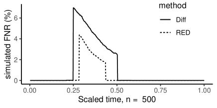
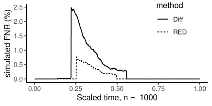
Figure 5.1: Solid lines and dotted lines denote time-varying simulated false negative rates of Algorithm 1(RED) and Algorithm 1(Diff), respectively. Left panel: $n=500$. Right panel: $n=1000$.

6 Data anaylsis

Since the financial crisis of 2007-2009, it has been widely recognized that network structures and connections are central to risk measurement, for example, the interconnectedness among assets, credit, and intersectoral input-output linkages are important for quantifying risks in financial portfolios, systemic and macroeconomic risks, respectively (see Puliga et al., (2014), Diebold and Yilmaz, (2014), Acemoglu et al., (2012) and reviews therein). Among others, Brunetti et al., (2019) classifies the financial network as ‘physical network’ and ‘correlation network’. The former is based on bank transactions and agent choices, while the latter, which is also the focus of this paper, is built on exploring correlation-related interactions among asset returns. Moreover, correlation networks are essentially time-varying and evolving which have been frequently investigated for the forecast of financial crises, see Diebold and Yilmaz, (2014). In this section, we analyze the time-varying correlation networks of Daily WRDS World Indices, which are market-capitalization weighted indices with dividends at daily frequency, see https://wrds-www.wharton.upenn.edu/pages/get-data/world-indices-wrds/ for details. Specifically, we investigate the weekly average of Daily Country Return with Dividends (PORTRET) from June 1st, 2006 to June 1st, 2022. There are 819 time points for each country. We denote the weekly average of the absolute value of PORTRET by $S_{i}$ and the weekly average of the squared logarithm of PORTRET by $R_{i}$, which are frequently employed as measures of volatility and risk. First, we examine the independent assumption for each country by testing for the autocorrelations of $R_{i}$ and $S_{i}$ of lags 1,2,3 simultaneously and find RED-SCBs reject the null hypotheses of zero serial correlations of $R_{i}$ of China and Germany, and $S_{i}$ of Germany, France, and Japan at the significance level of $0.5\%$, respectively. Hence, the independent assumption of classical methods can be restrictive for these time series of indices. To infer the underlying time-varying network structure from this data set that has complex dynamics and trends, we employ Algorithm 1 which is based on RED-SCBs. For better visualization of the time-varying nature of the connections, we display in the left panels of Figure 6.1 and Figure 6.2 the heatmaps of confidence levels (i.e., the smallest confidence level that the SCBs cover $g_{ijk}(t)\equiv 0$, $(i,j,k)\in\mathbb{B}$, $t\in[b,1-b]$). Notice that the correlation networks can be recovered from the heatmaps via linking two nodes where the corresponding confidence levels are greater than a pre-specified threshold, see the right panels of Figure 6.1 and Figure 6.2. For the sake of simplicity, we use CHN, HK, DE, GB, FR, and JP short for China, Hong Kong, Germany, the United Kingdom, France, and Japan. For brevity, Figure 6.1 and Figure 6.2 only display the time-varying networks with selected time points of June 1st of each year (the years with no connections are omitted), while Figure 1.1 shows the sub-graphs at important time points based on $S_{i}$. Since our inference results hold simultaneously over time, other time points of interest can also be visualized similarly. As shown in Figure 6.1, around 06/01/2012 and 06/01/2018 when Hong Kong witnessed stock market falls, there are major changes in the connections between Hong Kong and the rest of the world in terms of absolute market-capitalization weighted indices. By contrast, Japan maintained significant connections with Europe countries (GB, FR, and DE) from 2010 to 2018.

Figure 6.2 illustrates the time-varying cross-correlation networks constructed from $R_{i}$. The aforementioned stock market crashes of Hong Kong in 2012 and 2018 have been identified from these volatility networks of 2011 and 2017 when there are drastic decreases in confidence in the cross-correlations between Hong Kong and the rest of the world. In the year of 2012, a series of financial crises including the European debt crisis occurred, Standard$\&$Poor’s downgraded France and eight other eurozone countries, and connections among eurozone countries weakened in general. However, during the years of recovering from a series of financial crises, the interconnectedness between Japan and the United Kingdom remained relatively strong due to the favoring policies and relations, including the agreement to jointly develop weapons systems in 2012, led by Prime Minister David Cameron and the Brexit agreement on trading in 2016. Between 2012 and 2016 the confidence levels of connections between China and the United Kingdom or Japan also fell violently, which might be driven by changing diplomatic and trading relations among those pairs of countries.

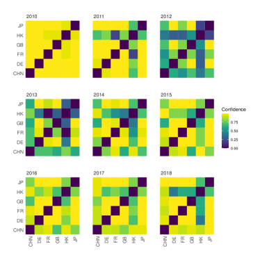
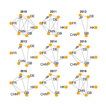
Figure 6.1: Left panel: the heatmap of confidence levels of cross-correlations of $S_{i}$ from 2010 to 2018 using Algorithm 1. Right panel: the snapshots of induced networks with threshold $0.9$.

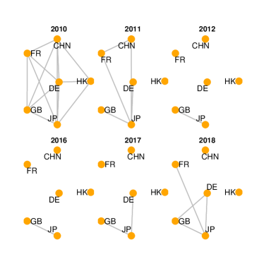
Figure 6.2: Left panel: the heatmap of confidence levels of cross-correlations of $R_{i}$ from 2010 to 2018 using Algorithm 1. Right panel: the snapshots of induced networks with threshold $0.85$, where networks with no connections are omitted.

7 Conclusion and future work

In this paper, we propose a unified framework for inferring time-varying cross-correlation networks from multivariate time series vectors with complex trends, where the dimension of the vectors and the number of correlation-based measures can be both fixed and divergent. We leverage the difference-based estimators to circumvent the pre-estimation of unknown change points in the piecewise smooth trends and develop a bootstrap-assisted approach to infer the time-varying network structures under time series nonstationarity. As a by-product, we bridge the gap of correlation inference between fixed and diverging lags in the time series literature. We improve the probability of recovering time-varying networks by extending the variance reduction technique for univariate time series nonparametric estimation to the uniform width reduction of SCBs for non-stationary and nonlinear time series. We provide theoretical justifications for our proposed bootstrap-assisted algorithms and evaluate the finite sample performance by simulations studies and the analysis of a financial data set.

The interconnectedness in the dynamic networks can be gauged by not only cross-correlations but also other measures such as Granger-causality, variance decomposition, and cross-quantilogram, see Andrieş et al., (2022) for a thorough review. Statistical properties of other measures for the inference of large-scale networks constructed from general and possibly nonlinear and non-stationary processes have not been thoroughly investigated yet. Besides FWER, the false discovery rate (FDR) is also a popular and powerful tool for multiple testing and building networks. We leave constructing networks through other measures or via other criteria including FDR as rewarding future work.

Appendix A Detailed formulae for Algorithms

This section gives the exact formulae of the estimators used in Algorithm 1 and Algorithm 1. Recall the definitions in Theorem 3.2, $\kappa=\int K^{2}(t)dt$, $\check{\kappa}=\int\check{K}^{2}(t)dt$.

A.1 Estimators for Algorithm 1

Recall that the definitions of $\check{\beta}_{z}(t)$, $\check{\gamma}^{i}_{0}(t)$, $\check{\sigma}_{i,l}(t)$, $\check{\rho}_{z}(t)$ and $\check{K}(t)$, $z=(i,l,k)\in\mathbb{B}$, $1\leq i,l\leq p$, in Section 2.2. Define the variance-reduced residuals $\hat{\check{e}}^{i,l}_{j,k}$ as $\tilde{y}_{j,k}^{i}\tilde{y}_{j,h}^{i}-\check{\beta}_{k}^{i,l}(t_{j})$. Then, the variance-reduced estimators of $\Xi_{z,j}$ and $\check{\Gamma}_{z}(t)$ are

$$\check{\Xi}_{z,j}=(\tilde{y}^{i}_{j,h}\tilde{y}^{l}_{j,h}/2-\tilde{y}^{i}_{j,k}\tilde{y}^{l}_{j,h})/\check{\sigma}_{i,l}(t)-4^{-1}\check{\rho}^{i,l}_{k}(t_{j})\left(\tilde{y}_{j,h}^{i,2}/\check{\gamma}^{i}_{0}(t_{j})+\tilde{y}_{j,h}^{l,2}/\check{\gamma}^{l}_{0}(t_{j})\right),$$ (A.1)

and

$$\hat{\check{\Gamma}}_{z}^{2}(t)=\frac{\check{\kappa}}{m}\sum_{i=1}^{n}\check{\Delta}^{2}_{z,i}\omega(t,i),\quad\omega(t,i)=K_{\eta}(t-t_{i})/\sum_{j=1}^{n}K_{\eta}(t_{j}-t),$$ (A.2)

where $\check{\Delta}_{z,s}=\sum_{j=s}^{s+m-1}\hat{\check{\Xi}}_{z,j}$, and $\hat{\check{\Xi}}_{z,j}=(\hat{\check{e}}^{i,l}_{j,h}/2-\hat{\check{e}}^{i,l}_{j,k})/\check{\sigma}_{i,l}(t)-4^{-1}\check{\rho}^{i,l}_{k}(t)\big{(}\hat{\check{e}}^{i}_{j,h}/\check{\gamma}^{i}_{0}(t_{j})+\hat{\check{e}}^{l}_{j,h}/\check{\gamma}^{l}_{0}(t_{j})\big{)}$. We then define $\hat{\check{\mathbf{\Xi}}}_{j}^{\mathbb{B}}$, $1\leq j\leq 2\lceil nb\rceil$, as

$$\hat{\check{\mathbf{\Xi}}}_{j}^{\mathbb{B}}=(\hat{\check{\mathbf{\Xi}}}_{j,\lceil nb\rceil}^{\mathbb{B},\top},\cdots,\hat{\check{\mathbf{\Xi}}}_{n-2\lceil nb\rceil+j,n-\lceil nb\rceil}^{\mathbb{B},\top})^{\top},~{}\text{with}~{}\hat{\check{\mathbf{\Xi}}}_{j,s}^{\mathbb{B}}=(c_{z}K_{b_{z}}(t_{j}-t_{s})\check{\Xi}_{z,j}/\hat{\check{\Gamma}}_{z}(t_{s}),z\in\mathbb{B})^{\top}.$$ (A.3)

Appendix B Time-varying cross-correlation analysis via difference-based SCBs

In this section, we list the algorithm based on difference-based SCBs without variance reduction, and provide the estimators therein and its theoretical properties.

Algorithm 1 Time-varying cross-correlation analysis

1:Compute $\tilde{\rho}^{i,l}_{k}(t)$, $(i,l,k)\in\mathbb{B}$ defined in (2.11).

2:Compute the $|\mathbb{B}|$-dimensional vectors $\hat{\bar{\mathbf{\Xi}}}_{j,s}^{\mathbb{B}}$ using (B.3), $1\leq j,s\leq n$.

3:For a window size $w$, compute $\hat{\tilde{\mathbf{S}}}_{l,j}^{\mathbb{B}}=\sum_{s=j-w+1}^{j}\hat{\bar{\mathbf{\Xi}}}_{s+l,\lceil nb\rceil+l}^{\mathbb{B}}-\sum_{s=j+1}^{j+w}\hat{\bar{\mathbf{\Xi}}}_{s+l,\lceil nb\rceil+l}^{\mathbb{B}}$, where $l=0,\cdots,n-2\lceil nb\rceil$.

4:for $r=1,\cdots,B$ do

5:     Generate independent standard normal random variables $R_{j}^{(r)}$, $j=1,\cdots,n$.

6:     Recall that $b=\max_{(i,l,k)\in\mathbb{B}}b^{i,l}_{k}$. Calculate

$$\tilde{Z}_{\mathrm{boot}}^{(r)}=\frac{\underset{0\leq l\leq n-2\lceil nb\rceil}{\max}\left|\sum_{j=w}^{2\lceil nb\rceil-w}\hat{\tilde{\mathbf{S}}}_{l,j}^{\mathbb{B}}R^{(r)}_{l+j}\right|_{\infty}}{\sqrt{2w\lceil nb\rceil}}.$$

7:end for

8:Let $\tilde{r}_{\mathrm{boot}}$ denote the $(1-\alpha)$-quantile of the bootstrap samples $\tilde{Z}_{\mathrm{boot}}^{(1)},\cdots,\tilde{Z}_{\mathrm{boot}}^{(B)}$.

9:Connect $i$ and $l$ at time $t\in[b,1-b]$ if $|g_{ilk}(t)-\tilde{\rho}^{i,l}_{k}(t)|>\tilde{r}_{\mathrm{boot}}(nb^{i,l}_{k})^{-1/2}\hat{\tilde{\Gamma}}^{i,l}_{k}(t)$ for some $k$ such that $(i,l,k)\in\mathbb{B}$.

B.1 Estimators

Recall that $\tilde{y}^{i}_{j,k}=Y_{j,i}-Y_{j-k,i}$. For the estimation of $\Xi_{z,j},z=(i,l,k)\in\mathbb{B}$ in (2.16), we use the following difference-based estimator:

$$\tilde{\Xi}_{z,j}=(\tilde{y}^{i}_{j,h}\tilde{y}^{l}_{j,h}/2-\tilde{y}^{i}_{j,k}\tilde{y}^{l}_{j,h})/\tilde{\sigma}_{i,l}(t_{j})-4^{-1}\tilde{\rho}^{i,l}_{k}(t_{j})\left(\tilde{y}_{j,h}^{i,2}/\tilde{\gamma}^{i}_{0}(t_{j})+\tilde{y}_{j,h}^{l,2}/\tilde{\gamma}^{l}_{0}(t_{j})\right).$$ (B.1)

Define the residuals of the local linear regression (2.8) as $\hat{\tilde{e}}^{i,l}_{j,k}=\tilde{y}_{j,k}^{i}\tilde{y}_{j,h}^{l}-\hat{\beta}_{k}^{i,l}(t_{j})$. For the estimation of ${\tilde{\Gamma}}_{z}^{2}(\cdot)$, we use

$$\hat{\tilde{\Gamma}}_{z}^{2}(t)=\frac{\kappa}{m}\sum_{i=1}^{n}\tilde{\Delta}^{2}_{z,i}\omega(t,i),\quad\omega(t,i)=K_{\eta}(t-t_{i})/\sum_{j=1}^{n}K_{\eta}(t_{j}-t),$$ (B.2)

where $\tilde{\Delta}_{z,s}=\sum_{j=s}^{s+m-1}\hat{\Xi}_{z,j}$, and $\hat{\Xi}_{z,j}=(\hat{\tilde{e}}^{i,l}_{j,h}/2-\hat{\tilde{e}}^{i,l}_{j,k})/\tilde{\sigma}_{i,l}(t)-4^{-1}\tilde{\rho}^{i,l}_{k}(t)\big{(}\hat{\tilde{e}}^{i}_{j,h}/\tilde{\gamma}^{i}_{0}(t_{j})+\hat{\tilde{e}}^{l}_{j,h}/\tilde{\gamma}^{l}_{0}(t_{j})\big{)}$. For $1\leq j\leq 2\lceil nb\rceil$, $\hat{\bar{\mathbf{\Xi}}}_{j}^{\mathbb{B}}$ is the estimator of $\bar{\mathbf{\Xi}}_{j}^{\mathbb{B}}$ (i.e., (2.16)) using estimators $\tilde{\Xi}_{z,j}$ and $\hat{\tilde{\Gamma}}_{z}^{2}(t)$ for $\Xi_{z,j}$ and ${\tilde{\Gamma}}_{z}^{2}(t)$, i.e.,

$$\quad\hat{\bar{\mathbf{\Xi}}}_{j}^{\mathbb{B}}=(\hat{\bar{\mathbf{\Xi}}}_{j,\lceil nb\rceil}^{\mathbb{B},\top},\cdots,\hat{\bar{\mathbf{\Xi}}}_{n-2\lceil nb\rceil+j,n-\lceil nb\rceil}^{\mathbb{B},\top})^{\top},~{}\text{with}~{}\hat{\bar{\mathbf{\Xi}}}_{j,s}^{\mathbb{B}}=(c_{z}K_{b_{z}}(t_{j}-t_{s})\tilde{\Xi}_{z,j}/\hat{\tilde{\Gamma}}_{z}(t_{s}),z\in\mathbb{B})^{\top}.$$ (B.3)

B.2 Theoretical properties

Write $\sqrt{nb_{z}}|g_{z}(t)-\tilde{\rho}_{z}(t)|/\hat{\tilde{\Gamma}}_{z}(t)$ as $\tilde{T}_{z}(t)$, $t\in[0,1]$. Then, the FWER (conditional on data) can be directly expressed as $1-P_{H_{0}}(\{\tilde{T}_{z}(t)\leq\tilde{r}_{\mathrm{boot}},z=(i,l,k)\in\mathbb{B},t\in[b,1-b]\}|\mathcal{F}_{n})$, where $H_{0}$ denotes the null hypotheses of (1.1). The recovery probability of time-varying networks conditional on data is

$$\quad\int_{0}^{1}P(\tilde{N}(t)|\mathcal{F}_{n})dt,$$ (B.4)

where $\tilde{N}(t)=\{\tilde{T}_{z}(t)\leq\tilde{r}_{\mathrm{boot}},z\in\mathbb{B}\cap\bar{\tilde{\mathbb{B}}}(t)\}\cap\{\tilde{T}_{z}(t)>\tilde{r}_{\mathrm{boot}},z\in\tilde{\mathbb{B}}(t)\}$. Define $\tilde{\mathcal{C}}_{n}=\{\mathbf{x}(\cdot)=(x_{z}(\cdot),z\in\mathbb{B})^{\top}\in[b,1-b]^{|\mathbb{B}|}:\sqrt{nb_{z}}|x_{z}(t)-\tilde{\rho}_{z}(t)|\leq\tilde{r}_{\mathrm{boot}}\hat{\tilde{\Gamma}}_{z}(t),\forall t\in[b,1-b],z\in\mathbb{B}\}$. Recall that $\alpha\in(0,1)$ is the prespecified significance level.

The following theorem ensures the FWER control and the recovery probability of Algorithm 1. The proof is deferred to Appendix C.

Theorem B.1.

Assume the conditions of Theorem 3.1 and

$$\vartheta_{n}^{1/3}\left(1\vee\log(n|\mathbb{B}|/\vartheta_{n})\right)^{2/3}+\big{(}g_{n}(n|\mathbb{B}|)^{1/q}\big{)}^{q/(q+2)}\to 0.$$ (B.5)

(i) (Type I error control.) Conditional on data as $n$ and $B$ go to infinity, we have

$$P_{H_{0}}(\{\tilde{T}_{z}(t)\leq\tilde{r}_{\mathrm{boot}},z\in\mathbb{B},t\in[b,1-b]\}|\mathcal{F}_{n})=P(\{\rho_{z}(\cdot),z\in\mathbb{B}\}\in\tilde{\mathcal{C}}_{n}|\mathcal{F}_{n})\overset{p}{\to}1-\alpha.$$ (B.6)

(ii) (The lower bound of the recovery probability.) Under 3.5, we have

$$\underset{n\to\infty}{\lim}\underset{B\to\infty}{\lim}\int_{0}^{1}P(\tilde{N}(t)|\mathcal{F}_{n})dt\geq 1-\alpha,$$

with probability approaching $1$ for any arbitrarily small $\alpha>0$, where $\tilde{N}(t)$ is the event for correctly recovering the network at time $t$, see (B.4).

B.3 Implementation

The selection of smoothing parameters for Algorithm 1 follows similarly to that of Algorithm 1. In particular, we use the same scheme for the selection of $b_{z}$, $m_{z}$, $z=(i,l,k)\in\mathbb{B}$ and for $w$ and $\eta$, while the sample variance $s^{2}_{w_{i},\eta_{j}}$ of (4.2) should be modified by replacing $\hat{\check{\mathbf{S}}}_{l,j}^{\mathbb{B}}$ with the variance-reduced estimator $\hat{\tilde{\mathbf{S}}}^{\mathbb{B}}_{l,j}$ of the Step 3 of Algorithm 1.

Appendix C Proofs

For the clarity of proof, we may use $(i,l,k)$ for $z$ in the index of correlations, bandwidths and estimators. Recall that $b=\max_{(i,l,k)\in\mathbb{B}}b^{i,l}_{k}$. For any two random sequences $a_{n}$ and $b_{n}$, let $a_{n}\sim_{1}b_{n}$ denote $\lim_{n\to\infty}a_{n}/b_{n}\to 1$ with probability approaching $1$, $a_{n}\lesssim_{1}b_{n}$ denote $\limsup_{n\to\infty}a_{n}/b_{n}\leq 1$ with probability approaching $1$. We use $a\vee b$ to denote $\max\{a,b\}$. Let $\Theta(a,b)=a\sqrt{1\vee\log(b/a)}$, where $a,b$ are positive constants. Let $\mathcal{T}=[b,1-b]$.

We present the necessary propositions used in the main paper and the proofs of the theorems, whose proofs can be found in Appendix F of the online supplement. Define the $\mathcal{F}_{n}$ measurable event

$$B^{\prime}_{n}=\left\{\max_{(i,l,k)\in\mathbb{B}}\sup_{t\in\mathcal{T}}\left|\tilde{\gamma}^{i,l}_{k}(t)-\gamma^{i,l}_{k}(t)\right|>f_{n}q_{n}^{\prime}\right\},$$

where $f_{n}=(nb)^{-1/2}(|\mathbb{B}|/b)^{1/q}$, $q_{n}^{\prime}$ is a positive sequence such that $q_{n}^{\prime}\to\infty$, $f_{n}q_{n}^{\prime}\to 0$.

Proposition C.1 (Asymptotic behavior of estimated cross-correlation curves).

Let $\mathcal{T}=[b,1-b]$. Under Assumptions 3.1, 3.2, 3.3, 3.4, and the bandwidth conditions $nb^{4}\to\infty$, $nb^{7}\to 0$, $n^{2\phi-1}b^{-1}h\to 0$, we have the following results:

1. Recall $\vartheta^{i,l}_{k}(t)=\frac{1}{nb_{k}^{i,l}}\sum_{j=1}^{n}K_{b_{k}^{i,l}}(t_{i}-t)\Xi^{i,l}_{j,k}$, where $\Xi^{i,l}_{j,k}$ is as defined in (2.16). Then, we have

   $$\max_{(i,l,k)\in\mathbb{B}}\left\|\sup_{t\in\mathcal{T}}\left|\tilde{\rho}^{i,l}_{k}(t)-\rho^{i,l}_{k}(t)-\vartheta^{i,l}_{k}(t)\right|\mathbf{1}(\bar{B}^{\prime}_{n})\right\|_{q}=O\left(n^{\phi-1}b^{-1-1/q}h+b^{3-1/q}+n^{-1/2}b^{-1/q}h\right).$$

2. Recall that $\check{\vartheta}^{i,l}_{k}(t):=\frac{1}{nb_{k}^{i,l}}\sum_{j=1}^{n}\check{K}_{b_{k}^{i,l}}(t_{i}-t)\Xi^{i,l}_{j,k}$. Then, we have

   $$\max_{(i,l,k)\in\mathbb{B}}\left\|\sup_{t\in\mathcal{T}}\left|\check{\rho}_{k}^{i,l}(t)-\rho^{i,l}_{k}(t)-\check{\vartheta}^{i,l}_{k}(t)\right|\mathbf{1}(\bar{B}^{\prime}_{n})\right\|_{q}=O\left(n^{\phi-1}b^{-1-1/q}h+b^{3-1/q}+n^{-1/2}b^{-1/q}h\right).$$ (C.1)

Proposition C.2.

Under the condition of Proposition C.1, assuming bandwidth conditions $\eta\to 0$, $n\eta\to\infty$, $m\to\infty$, $m=O(n^{1/3})$, $|\mathbb{B}|^{1/q}(mb/n)^{-1/(2q)}\sqrt{m/(nb)}\to 0$, $nb^{3}\to\infty$, $nb^{6}\to 0$. Suppose for $(i,l,k)\in\mathbb{B}$, the twice derivatives of $\tilde{\Gamma}^{i,l,2}_{k}(t)$ are uniformly bounded on $(0,1)$. Then, we have

$$\left\|\max_{(i,l,k)\in\mathbb{B}}\sup_{t\in\mathcal{T}}\left|\hat{\tilde{\Gamma}}^{i,l,2}_{k}(t)-\tilde{\Gamma}^{i,l,2}_{k}(t)\right|\right\|_{q}=O\left(|\mathbb{B}|^{1/q}g_{n}^{\prime}\right),$$ (C.2)

where $g_{n}^{\prime}=\sqrt{m/(n\eta^{2})}+1/m+\eta+\sqrt{m/(nb)}(mb/n)^{-1/(2q)}$.

C.1 Proof of Theorem B.1

Let $\tilde{Z}_{\mathrm{boot}}$ denote $\tilde{Z}^{(r)}_{\mathrm{boot}}$ in one iteration of Algorithm 1. By Theorem 3.1, it’s sufficient to show that

$$\sup_{x\in\mathbb{R}}\left|P(\tilde{Z}_{\mathrm{boot}}\leq x|\mathcal{F}_{n})-P\left(\left|\frac{1}{\sqrt{nb}}\sum_{i=1}^{2\lceil nb\rceil}\tilde{\mathbf{Z}}_{i}\right|_{\infty}\leq x\right)\right|=o_{\mathbb{P}}(1),$$ (C.3)

where $(\tilde{\mathbf{Z}}_{i})_{i=1}^{2\lceil nb\rceil}\in\mathbb{R}^{(n-2\lceil nb\rceil+1)|\mathbb{B}|}$ is a sequence of zero-mean Gaussian vectors which share the same autocovariance structure with the vectors $(\bar{\mathbf{\Xi}}^{\mathbb{B}}_{i})_{i=1}^{2\lceil nb\rceil}$ as defined in Theorem 3.1. In the following proof, we omit the index $\mathbb{B}$ in $\hat{\tilde{\mathbf{S}}}^{\mathbb{B}}_{l,j}$ for simplicity. Define

$$\tilde{\mathbf{Z}}^{\diamond}_{a|\mathbb{B}|+c}=\left((2w\lceil nb\rceil)^{-1/2}\sum_{j=w}^{2\lceil nb\rceil-w}\hat{\tilde{S}}_{a-1,j,c}R_{a+j-1},a=1,\cdots,n-2\lceil nb\rceil+1,1\leq c\leq|\mathbb{B}|\right),$$ (C.4)

where $\hat{\tilde{S}}_{l,j,r}$ denote the $r$th element of $\hat{\tilde{\mathbf{S}}}_{l,j}$. Let

$$\tilde{\mathbf{Z}}^{\diamond}=\left(\tilde{\mathbf{Z}}_{1}^{\diamond,\top},\cdots,\tilde{\mathbf{Z}}_{(n-2\lceil nb\rceil+1)|\mathbb{B}|}^{\diamond,\top}\right)^{\top},$$ (C.5)

and it follows that $\tilde{Z}_{\mathrm{boot}}=|\tilde{\mathbf{Z}}^{\diamond}|_{\infty}$. Given the data, the conditional variance for $k_{1}\leq k_{2}$ is

$$\sigma^{\tilde{\mathbf{Z}}^{\diamond}}_{k_{1},k_{2},j_{1},j_{2}} :=(2w\lceil nb\rceil)^{-1}\mathbb{E}\left(\sum_{j=w}^{2\lceil nb\rceil-w}\hat{\tilde{S}}_{k_{1}-1,j,j_{1}}R_{k_{1}-1+j}\sum_{j=w}^{2\lceil nb\rceil-w}\hat{\tilde{S}}_{k_{2}-1,j,j_{2}}R_{k_{2}-1+j}|\mathcal{F}_{n}\right)$$ (C.6)

$$=\sum_{j=w}^{2\lceil nb\rceil-w-(k_{2}-k_{1})-1}\hat{\tilde{S}}_{k_{1}-1,j+k_{2}-k_{1},j_{1}}\hat{\tilde{S}}_{k_{2}-1,j,j_{2}}/(2w\lceil nb\rceil).$$ (C.7)

Define $\bar{\Xi}_{i,s,j}^{\mathbb{B}}$ as the $j$th element of $\mathbf{\bar{\Xi}}_{i,s}^{\mathbb{B}}$. For simplicity, we omit the index $\mathbb{B}$ in $\bar{\Xi}_{i,s,j}^{\mathbb{B}}$. Define

$$\tilde{S}_{a-1,j,c}=\sum_{i=j-w+1}^{j}\bar{\Xi}_{i+(a-1),\lceil nb\rceil+(a-1),c}-\sum_{i=j+1}^{j+w}\bar{\Xi}_{i+(a-1),\lceil nb\rceil+(a-1),c},$$ (C.8)

and $\tilde{\mathbf{Z}}^{\dagger}$ by substituting $\hat{\tilde{S}}_{(a-1),j,c}$ in $\tilde{\mathbf{Z}}^{\diamond}$ by $\tilde{S}_{(a-1),j,c}$.

$$\sigma^{\tilde{\mathbf{Z}}^{\dagger}}_{k_{1},k_{2},j_{1},j_{2}} :=(2w\lceil nb\rceil)^{-1}\mathbb{E}\left(\sum_{j=w}^{2\lceil nb\rceil-w}\tilde{S}_{k_{1}-1,j,j_{1}}R_{k_{1}-1+j}\sum_{j=w}^{2\lceil nb\rceil-w}\tilde{S}_{k_{2}-1,j,j_{2}}R_{k_{2}-1+j}|\mathcal{F}_{n}\right)$$ (C.9)

$$=\sum_{j=w}^{2\lceil nb\rceil-w-(k_{2}-k_{1})}\tilde{S}_{k_{1}-1,j+k_{2}-k_{1},j_{1}}\tilde{S}_{k_{2}-1,j,j_{2}}/(2w\lceil nb\rceil).$$ (C.10)

Let $\tilde{Z}_{i,j}$ denote the $j$th element of $\tilde{\mathbf{Z}}_{i}$ . Since $\tilde{\mathbf{Z}}_{i}$ has the same covariance structure as $\bar{\mathbf{\Xi}}_{i}^{\mathbb{B}}$, the covariance structure of $\frac{1}{\lceil nb\rceil}\sum_{i=1}^{2\lceil nb\rceil}\tilde{\mathbf{Z}}_{i}$ is

$$\sigma^{\tilde{\mathbf{Z}}}_{k_{1},k_{2},j_{1},j_{2}} :=\mathbb{E}\left(\frac{1}{\lceil nb\rceil}\sum_{i=1}^{2\lceil nb\rceil}\tilde{Z}_{i,(k_{1}-1)|\mathbb{B}|+j_{1}}\sum_{i=1}^{2\lceil nb\rceil}\tilde{Z}_{i,(k_{2}-1)|\mathbb{B}|+j_{2}}\right)$$ (C.11)

$$=\mathbb{E}\left(\frac{1}{\lceil nb\rceil}\sum_{i=1}^{2\lceil nb\rceil}\bar{\Xi}_{i+(k_{1}-1),\lceil nb\rceil+(k_{1}-1),j_{1}}\sum_{i=1}^{2\lceil nb\rceil}\bar{\Xi}_{i+(k_{2}-1),\lceil nb\rceil+(k_{2}-1),j_{2}}\right).$$ (C.12)

By (5.12) of Dette and Wu, (2021), since $(\bar{\Xi}^{i,l}_{j,k})_{j=1}^{n}$ are LS and satisfy geometric metric contraction due to 3.1, we have

$$\left\|\max_{k_{1},k_{2},j_{1},j_{2}}|\sigma^{\tilde{\mathbf{Z}}^{\dagger}}_{k_{1},k_{2},j_{1},j_{2}}-\sigma^{\tilde{\mathbf{Z}}}_{k_{1},k_{2},j_{1},j_{2}}|\right\|_{q/2}=O\left(\frac{\log^{2}n}{w}+\frac{w}{nb}+\sqrt{\frac{w}{nb}}(n\log n)^{4/q}\right).$$ (C.13)

By (5.12) and (5.13) of Dette and Wu, (2021), we have

$$\sup_{x\in\mathbb{R}}\left|P\left(\left.|\tilde{\mathbf{Z}}^{\dagger}|\leq x\right|\mathcal{F}_{n}\right)-P\left(\left|\frac{1}{\sqrt{nb}}\sum_{i=1}^{2\lceil nb\rceil}\tilde{\mathbf{Z}}_{i}\right|_{\infty}\leq x\right)\right|=O_{\mathbb{P}}(\vartheta_{n}^{1/3}\left\{1\vee\log(n|\mathbb{B}|/\vartheta_{n})\right\}^{2/3}),$$ (C.14)

where $\vartheta_{n}=\frac{\log^{2}n}{w}+\frac{w}{nb}+\sqrt{\frac{w}{nb}}(n\log n)^{4/q}$. Let $g^{\prime}_{n}=|\mathbb{B}|^{1/q}(\sqrt{m/(n\eta^{2})}+1/m+\eta+\sqrt{m/(nb)}(mb/n)^{-1/2q})$, $f_{n}=(nb)^{-1/2}b^{-1/q}|\mathbb{B}|^{1/q}$. Recall the estimators $\tilde{\rho}^{i,l}_{k}(\cdot)$ and $\hat{\tilde{\Gamma}}^{i,l,2}_{k}(\cdot)$ as defined in (2.11) and (B.2), respectively. Define the $\mathcal{F}_{n}$ measurable events

$$A_{n}=\left\{\max_{(i,l,k)\in\mathbb{B}}\sup_{t\in\mathcal{T}}\left|\hat{\tilde{\Gamma}}^{i,l,2}_{k}(t)-\tilde{\Gamma}^{i,l,2}_{k}(t)\right|>g^{\prime}_{n}q_{n}\right\},\quad B_{n}=\left\{\max_{(i,l,k)\in\mathbb{B}}\sup_{t\in\mathcal{T}}\left|\tilde{\beta}^{i,l}_{k}(t)-\beta^{i,l}_{k}(t)\right|>f_{n}q_{n}\right\},$$ (C.15)

where the positive sequence $q_{n}$ goes to infinity such that $(g_{n}^{\prime}+f_{n})q_{n}\to 0$, $\mathcal{T}=[b,1-b]$. Then by Lemma 1 and Proposition C.2, $P(A_{n}\cup B_{n})=O(q_{n}^{-q})$. Then, for some sufficiently large constant $M$ and due to the conditional normality, we have

$$\mathbb{E}(|\tilde{\mathbf{Z}}^{\diamond}-\tilde{\mathbf{Z}}^{\dagger}|^{q}_{\infty}\mathbf{1}(\bar{A}_{n}\cap\bar{B}_{n})|\mathcal{F}_{n})\leq M\left|\frac{\log(n|\mathbb{B}|)}{2w\lceil nb\rceil}\max_{\begin{subarray}{c}1\leq r\leq|\mathbb{B}|\\ 0\leq l\leq n-2\lceil nb\rceil\end{subarray}}\sum_{j=w}^{2\lceil nb\rceil-w}(\hat{\tilde{S}}_{l,j,r}-\tilde{S}_{l,j,r})^{2}\mathbf{1}(\bar{A}_{n}\cap\bar{B}_{n})\right|^{q/2}.$$ (C.16)

Recall the definition of $\hat{\bar{\mathbf{\Xi}}}_{i+l,\lceil nb\rceil+l}^{\mathbb{B}}$ in (B.3). Let $\hat{\bar{\Xi}}_{i+l,\lceil nb\rceil+l,r}$ denote the $r$th element of $\hat{\bar{\mathbf{\Xi}}}_{i+l,\lceil nb\rceil+l}^{\mathbb{B}}$. Define $\hat{\tilde{S}}^{\epsilon}_{a,j,r}$ by substituting $\tilde{y}^{i}_{j,k}$ in $\hat{\tilde{S}}_{a,j,r}$ with $\tilde{\epsilon}^{i}_{j,k}$, $\hat{\tilde{S}}^{e}_{a,j,r}$ by substituting $\tilde{\epsilon}^{i}_{j,k}\tilde{\epsilon}^{l}_{j,h}$ in $\hat{\tilde{S}}^{\epsilon}_{a,j,r}$ with $\tilde{e}^{i,l}_{j,k}$, $\hat{\tilde{S}}^{e,\Gamma}_{a,j,r}$ by substituting $\hat{\tilde{\Gamma}}^{i,l}_{k}(t)$ in $\hat{\tilde{S}}^{e}_{a,j,r}$ with ${\tilde{\Gamma}}^{i,l}_{k}(t)$ , and $\hat{\tilde{S}}^{e,\Gamma,\rho}_{a,j,r}$ by substituting $\tilde{\rho}^{i,l}_{k}(t)$ in $\hat{\tilde{S}}^{e,\Gamma}_{a,j,r}$ with $\rho^{i}_{j,k}(t)$. Note that $\hat{\tilde{S}}^{e,\Gamma}_{a,j,r}=\tilde{S}_{l,j,r}$. By the continuity of $\beta^{i,l}_{k}(\cdot)$, via the proof of Proposition C.1 , we have

$$\frac{1}{\sqrt{2w\lceil nb\rceil}}\left\|\max_{\begin{subarray}{c}1\leq r\leq|\mathbb{B}|\\ 0\leq l\leq n-2\lceil nb\rceil\end{subarray}}\left(\sum_{j=w}^{2\lceil nb\rceil-w}(\hat{\tilde{S}}_{l,j,r}-\tilde{S}_{l,j,r})^{2}\mathbf{1}(\bar{A}_{n}\cap\bar{B}_{n})\right)^{1/2}\right\|_{q}$$ (C.17)

$$\leq\frac{C(n|\mathbb{B}|)^{1/q}}{\sqrt{2w\lceil nb\rceil}}\max_{\begin{subarray}{c}1\leq r\leq|\mathbb{B}|\\ 0\leq l\leq n-2\lceil nb\rceil\end{subarray}}\left|\sum_{j=w}^{2\lceil nb\rceil-w}\left(\|\hat{\tilde{S}}_{l,j,r}-\hat{\tilde{S}}^{\epsilon}_{l,j,r})\|_{q}^{2}+\|\hat{\tilde{S}}^{\epsilon}_{l,j,r}-\hat{\tilde{S}}^{e}_{l,j,r}\|_{q}^{2}\right.\right.$$ (C.18)

$$\left.\left.+\|\hat{\tilde{S}}^{e}_{l,j,r}-\hat{\tilde{S}}^{e,\Gamma}_{l,j,r}\|_{q}^{2}+\|\hat{\tilde{S}}^{e,\Gamma}-\tilde{S}_{l,j,r}\|_{q}^{2}\right)\mathbf{1}(\bar{A}_{n}\cap\bar{B}_{n})\right|^{1/2}$$ (C.19)

$$=O((n^{\phi}h/\sqrt{w}+w^{3/2}/n+g^{\prime}_{n}q_{n}+f_{n}q_{n})(n|\mathbb{B}|)^{1/q}),$$ (C.20)

where $C$ is a sufficiently large constant, and the last inequality is due to triangle inequality. Let $q_{n}=\left\{\left(g^{\prime}_{n}+f_{n}+w^{3/2}/n+n^{\phi}h/\sqrt{w}\right)(n|\mathbb{B}|)^{1/q}\right\}^{-1/(q+2)}$. Under (3.5), we have $q_{n}\to\infty$, and $(g_{n}^{\prime}+f_{n})q_{n}\leq g_{n}q_{n}\to 0$. By (C.14), (C.16) and (C.20), Lemma C.1 of Dette and Wu, (2021), we have shown (C.3), i.e.,

$$\sup_{x\in\mathbb{R}}\left|P(\tilde{Z}_{\mathrm{boot}}\leq x|\mathcal{F}_{n})-P\left(\left|\frac{1}{\sqrt{nb}}\sum_{i=1}^{2\lceil nb\rceil-1}\tilde{\mathbf{Z}}_{i}\right|_{\infty}\leq x\right)\right|$$ (C.21)

$$=O_{\mathbb{P}}\left(\vartheta_{n}^{1/3}\left\{1\vee\log(n|\mathbb{B}|/\vartheta_{n})\right\}^{2/3}+\Theta\left(q_{n}^{-q},n|\mathbb{B}|\right)\right).$$ (C.22)

Under 3.5, for $t\in[b,1-b]$, $z=(i,l,k)\in\tilde{\mathbb{B}}(t)$, by the concentration inequality of high-dimensional Gaussian process, we have uniformly

$$\sqrt{nb_{z}}|\tilde{\rho}_{z}(t)-g_{z}(t)|/\hat{\tilde{\Gamma}}_{z}(t) \geq\sqrt{nb_{z}}|g_{z}(t)-\rho_{z}(t)|/\hat{\tilde{\Gamma}}_{z}(t)-\max_{z\in\mathbb{B}}\sup_{t\in\mathcal{T}}\sqrt{nb_{z}}|\tilde{\rho}_{z}(t)-\rho_{z}(t)|/\hat{\tilde{\Gamma}}_{z}(t)$$ (C.23)

$$\geq\lambda_{n}\log(n|\mathbb{B}|)-O_{\mathbb{P}}(\log(n|\mathbb{B}|))\to\infty.$$ (C.24)

Combining (B.6) and (C.24), under 3.5, it follows that $\underset{n\to\infty}{\lim}\underset{B\to\infty}{\lim}\int_{0}^{1}P(\{\tilde{T}_{z}(t)\leq\tilde{r}_{\mathrm{boot}},z\in\mathbb{B}\cap\bar{\tilde{\mathbb{B}}}(t)\}\cap\{\tilde{T}_{z}(t)>\tilde{r}_{\mathrm{boot}},z\in\tilde{\mathbb{B}}(t)\}|\mathcal{F}_{n})dt\geq\underset{n\to\infty}{\lim}\underset{B\to\infty}{\lim}P(\{\rho_{z}(\cdot),z\in\mathbb{B}\}\in\tilde{\mathcal{C}}_{n}|\mathcal{F}_{n})=1-\alpha$, with probability approaching $1$. $\Box$

C.2 Proof of Theorem 3.2

Proof of (i). The result follows from Proposition C.1 and similar arguments in the proof of Theorem B.1.
Proof of (ii). After a further investigation of (C.24), we have $\left|\sqrt{nb_{z}}|\check{\rho}_{z}(t)-g_{z}(t)|-\sqrt{nb_{z}}|\tilde{\rho}_{z}(t)-g_{z}(t)|\right|=O_{\mathbb{P}}(\log(n|\mathbb{B}|))=o_{\mathbb{P}}(\lambda_{n})$. Therefore, if (3.8) holds, (3.7) will follow from Theorem B.1 and elementary calculation for a sufficiently small $\alpha$. In the following we shall prove (3.8). By Proposition C.2, we have

$$\max_{z\in\mathbb{B}}\sup_{t\in\mathcal{T}}\left|\hat{\check{\Gamma}}_{z}(t)/\hat{\tilde{\Gamma}}_{z}(t)-{\check{\Gamma}}_{z}(t)/\tilde{\Gamma}_{z}(t)\right|=o_{\mathbb{P}}(1).$$ (C.25)

Write $\Xi_{j,k}^{i,l}=\tilde{L}^{i,l}_{k}(t_{j},\mathcal{F}_{j})$, where $\tilde{L}^{i,l}_{k}(\cdot,\cdot)$ is a nonlinear filter, $(i,l,k)\in\mathbb{B}$. By a careful investigation of Lemma C.3 of Dette and Wu, (2022), we have $\tilde{\Gamma}_{k}^{i,l,2}(t)=\kappa\sigma^{2}(\tilde{L}^{i,l}_{k},t)$ and $\check{\Gamma}_{k}^{i,l,2}(t)=\check{\kappa}\sigma^{2}(\tilde{L}^{i,l}_{k},t)$, where $\sigma^{2}(\tilde{L}^{i,l}_{k},t)$ is the long-run variance of $\tilde{L}^{i,l}_{k}(t,\mathcal{F}_{j})$. Recall that $\check{K}(t)=(\check{K}_{+}(t)+\check{K}_{-}(t))/2$ where $\check{K}_{\pm}(t)=\sum_{j=0,1,2}A_{j}(\pm r)K(t+(\pm r+1-j)\delta)$, $A_{0}(r)=r(r-1)/2,A_{1}(r)=\left(1-r^{2}\right),A_{2}(r)=r(r+1)/2$ for some selected $r\in(-1,1)$ and non-negative constant $\delta$. It follows from the elementary calculation that

$$\int\check{K}^{2}(t)dt=\int K^{2}(t)dt-r^{2}(1-r^{2})C(\delta)-\frac{1}{2}D(\delta),$$ (C.26)

where $C(\delta)=1.5C(0,\delta)-2C(0.5,\delta)+0.5C(1,\delta)$, $C(a,\delta)=\frac{1}{2}\int K(u-a\delta)K(u+a\delta)+K(u-a\delta)K(u+a\delta)du$ and $D(\delta)=\kappa-r^{2}(1-r^{2})C(\delta)-\frac{1}{4}\{2(2-3r^{2})(1-r^{2})C(r,\delta)+r^{2}(1-r)^{2}C(r+1,\delta)+r^{2}(r+1)^{2}C(r-1,\delta)-4r(1-r)(1-r^{2})C(r+1/2,\delta)+4r(1+r)(1-r^{2})C(r-1/2,\delta)\}.$ The positivity of $C(\delta)$ and $D(\delta)$ when $\delta>0$ follows from 3.2 and a careful investigation of Proposition 1 and Proposition 2 of Cheng et al., (2007).

For a pre-specified significance level $0<\alpha<1$, we shall show $|\tilde{r}_{\mathrm{boot}}/\check{r}_{\mathrm{boot}}-1|=o_{\mathbb{P}}(1)$ by proving

$$|\tilde{r}_{\mathrm{boot}}-\sqrt{2\log b^{-1}}|=o_{\mathbb{P}}(1),\quad|\check{r}_{\mathrm{boot}}-\sqrt{2\log b^{-1}}|=o_{\mathbb{P}}(1).$$ (C.27)

We only give the proof for $\tilde{r}_{\mathrm{boot}}$ for brevity, and that of $\check{r}_{\mathrm{boot}}$ will follow similarly. Write $\tilde{r}$ short for $\tilde{r}_{\mathrm{boot}}$. We shall first show that uniformly for $x>\sqrt{2\log b^{-1}-2c}$ for some arbitrary non-negative $c$,

$$P(\tilde{Z}_{\mathrm{boot}}>x|\mathcal{F}_{n}) \geq\prod_{z\in\mathbb{B}}(b^{-1}c_{z}^{2}C_{\kappa}\exp(-x^{2}/2)+2(1-\Phi(x)))+o_{\mathbb{P}}(1)$$ (C.28)

$$\geq(b^{-1}C_{\kappa}\exp(-x^{2}/2)+2(1-\Phi(x)))^{|\mathbb{B}|}+o_{\mathbb{P}}(1).$$ (C.29)

where $C_{\kappa}=\sqrt{\int|K^{\prime}(x)|^{2}dx/\int K^{2}(x)dx}$. Recall that $P(\tilde{Z}_{\mathrm{boot}}>\tilde{r}|\mathcal{F}_{n})=1-\alpha$. Hence, (C.29) will lead to $\tilde{r}^{-}:=\sqrt{2\log(b^{-1}C_{\kappa})-2|\mathbb{B}|^{-1}\log\alpha}\lesssim_{1}\tilde{r}$. Recall the definition of $c^{*}$ in 3.3. On the other hand, we shall show that under 3.3, for any $x$ such that $x/\sqrt{2\log\log n}\to\infty$,

$$P(\tilde{Z}_{\mathrm{boot}}>x|\mathcal{F}_{n}) \leq 1-\prod_{z\in\mathbb{B}}(1-b^{-1}c_{z}^{2}C_{\kappa}\exp(-x^{2}/2)-2(1-\Phi(x)))+o_{\mathbb{P}}(1),$$ (C.30)

$$\leq 1-(1-b^{-1}(c^{*})^{-1}C_{\kappa}\exp(-x^{2}/2)-2(1-\Phi(x)))^{|\mathbb{B}|}+o_{\mathbb{P}}(1),$$ (C.31)

which will lead to $\tilde{r}\lesssim_{1}\sqrt{2\log(b^{-1}C_{\kappa}/c^{*})-2\log(1-(1-\alpha)^{1/|\mathbb{B}|})}=:\tilde{r}^{+}$. Since $|\mathbb{B}|^{-1}\log\alpha=o(b^{-1})$, $-\log(1-(1-\alpha)^{1/|\mathbb{B}|})=O(\log|\mathbb{B}|)=o(b^{-1})$, we have $\tilde{r}^{-}\sim_{1}\sqrt{2\log b^{-1}}$ and $\tilde{r}^{+}\sim_{1}\sqrt{2\log b^{-1}}$, which yields the result $|\tilde{r}-\sqrt{2\log b^{-1}}|=o_{\mathbb{P}}(1)$. Finally, after a further investigation of (C.24), we have $\left|\sqrt{nb_{z}}|\check{\rho}_{z}(t)-g_{z}(t)|-\sqrt{nb_{z}}|\tilde{\rho}_{z}(t)-g_{z}(t)|\right|=O_{\mathbb{P}}(\log(n|\mathbb{B}|))=o_{\mathbb{P}}(\lambda_{n}\log(n|\mathbb{B}|)).$ Since we have shown that $\hat{\check{\Gamma}}_{z}(t)/\hat{\tilde{\Gamma}}_{z}(t)\overset{p}{\to}\sqrt{\check{\kappa}/\kappa}<1$ and $|\tilde{r}_{\mathrm{boot}}/\check{r}_{\mathrm{boot}}-1|=o_{\mathbb{P}}(1)$, (3.7) then follows from (B.6) and result (i).

Proof of (C.29) and (C.31). By Theorem B.1, the tail probabilities of $\tilde{Z}_{\mathrm{boot}}$ and $\check{Z}_{\mathrm{boot}}$ given data are asymptotically equal to

$$P\left(\left|\frac{1}{\sqrt{nb}}\sum_{i=1}^{2\lceil nb\rceil}\tilde{\mathbf{Z}}_{i}\right|_{\infty}>x\right)~{}\text{and}~{}P\left(\left|\frac{1}{\sqrt{nb}}\sum_{i=1}^{2\lceil nb\rceil}\check{\mathbf{Z}}_{i}\right|_{\infty}>x\right),$$ (C.32)

uniformly over $x\in\mathbb{R}$ with probability approaching $1$, see (C.3). In the subsequent proof, we will derive explicit approximation formulae for the tail probabilities defined in (C.32). For brevity, we only present the details for the computation of the lower and upper bounds of $P\left(\left|\frac{1}{\sqrt{nb}}\sum_{i=1}^{2\lceil nb\rceil}\tilde{\mathbf{Z}}_{i}\right|_{\infty}>x\right)$, and the results for the variance reduced tail probability (the second term) in (C.32) follow analogously. Recall $\tilde{Z}_{i,j}$ is the $j$ th element in $\tilde{\mathbf{Z}}_{i}$. Define $\bar{\tilde{Z}}_{i,j}$ as $\tilde{Z}_{i,j}/\sqrt{\mathrm{Var}(\sum_{i=1}^{2\lceil nb\rceil}\tilde{Z}_{i,j})/(nb)}.$ By elementary calculation similar to Lemma C.3 in Dette and Wu, (2021), $\mathrm{Var}(\sum_{i=1}^{2\lceil nb\rceil}\tilde{Z}_{i,j})/(nb)$ is bounded from $0$, so that $\frac{1}{\sqrt{nb}}\sum_{i=1}^{2\lceil nb\rceil}\bar{\tilde{\mathbf{Z}}}_{i}$ is the normalized version of $\frac{1}{\sqrt{nb}}\sum_{i=1}^{2\lceil nb\rceil}{\tilde{\mathbf{Z}}}_{i}$ and each component is of variance $1$.

Proof of (C.29). We shall break the proof into the following 3 steps. Fix the order of the elements of $\mathbb{B}$, and let $z$ be the $j_{th}$ element of $\mathbb{B}$ in the following proofs.

Step 1: Under 3.6, when $|\mathbb{B}|=O(\log n)$, we shall show that for $x>\sqrt{2\log b^{-1}-2c}$, where $c$ is an arbitrary non-negative constant,

$$P\left(\left|\frac{1}{\sqrt{nb}}\sum_{i=1}^{2\lceil nb\rceil}\bar{\tilde{\mathbf{Z}}}_{i}\right|_{\infty}\leq x\right)\leq\prod_{j=1}^{|\mathbb{B}|}P\left(\max_{0\leq s\leq m^{*}}\left|\frac{1}{\sqrt{nb}}\sum_{i=1}^{2\lceil nb\rceil}\bar{\tilde{Z}}_{i,s\lceil nb\rceil|\mathbb{B}|+j}\right|\leq x\right)+o(1),$$ (C.33)

where $m^{*}=(n-2\lceil nb\rceil)/(\lceil nb\rceil)$.

Step 2: For $i.i.d.$ $N(0,1)$ random variables $v_{z,j}$, $z\in\mathbb{B}$, $1\leq j\leq n$, for $b\to 0$, $nb\to\infty$, we obtain

$$\sup_{x\in\mathbb{R}}\left|\prod_{j=1}^{|\mathbb{B}|}P\left(\max_{0\leq s\leq m^{*}}\left|\frac{1}{\sqrt{nb}}\sum_{i=1}^{2\lceil nb\rceil}\bar{\tilde{Z}}_{i,s\lceil nb\rceil|\mathbb{B}|+j}\right|\leq x\right)\right.$$ (C.34)

$$\left.-\prod_{z\in\mathbb{B}}P\left(\max_{0\leq s\leq m^{*}}\left|\sum_{i=1}^{2\lceil nb\rceil}\frac{v_{z,i+s\lceil nb\rceil}K_{b_{z}}(\frac{i-\lceil nb\rceil}{n})}{\sqrt{nb_{z}\kappa}}\right|\leq x\right)\right|=o(1).$$ (C.35)

Step 3: Show that for $x>\sqrt{2\log b^{-1}-2c}$, for the constant $c$ defined in Step 1

$$\prod_{z\in\mathbb{B}}P\left(\max_{0\leq s\leq m^{*}}\left|\sum_{i=1}^{2\lceil nb\rceil}\frac{v_{z,i+s\lceil nb\rceil}K_{b_{z}}(\frac{i-\lceil nb\rceil}{n})}{\sqrt{nb_{z}\kappa}}\right|>x\right)$$ (C.36)

$$=\prod_{z\in\mathbb{B}}(b^{-1}c_{z}^{2}C_{\kappa}\exp(-x^{2}/2)+2(1-\Phi(x)))+o(1),$$ (C.37)

where $\Phi(x)$ is the cumulative function of normal distribution, $C_{\kappa}=\sqrt{\int|K^{\prime}(x)|^{2}dx/\int K^{2}(x)dx}$. Therefore, since $c_{z}\geq 1$, (C.29) follows from (C.37).

Remark C.1.

$|\mathbb{B}|$ can also be allowed to diverge at a polynomial rate, such that $|\mathbb{B}|=o\left(b^{-\frac{1-\rho}{4(1+\rho)}}\right)$. We omit its proof for the sake of conciseness.

Proof of Step 1. When $|\mathbb{B}|$ is finite, the proof follows from Theorem 3 of Hüsler and Schüpbach, (1988). We extend it for diverging $|\mathbb{B}|$. Note that

$$P\left(\left|\frac{1}{\sqrt{nb}}\sum_{i=1}^{2\lceil nb\rceil}\bar{\tilde{\mathbf{Z}}}_{i}\right|_{\infty}\leq x\right)\leq P\left(\max_{1\leq j\leq|\mathbb{B}|,0\leq s\leq m^{*}}\left|\frac{1}{\sqrt{nb}}\sum_{i=1}^{2\lceil nb\rceil}\bar{\tilde{Z}}_{i,s\lceil nb\rceil|\mathbb{B}|+j}\right|\leq x\right).$$ (C.38)

For the sake of simplicity, let

$$J_{k,j}:=\frac{1}{\sqrt{nb}}\sum_{i=1}^{2\lceil nb\rceil}\bar{\tilde{Z}}_{i,(k-1)|\mathbb{B}|+j},\quad k=1,\cdots,n-2\lceil nb\rceil+1,j=1,\cdots,|\mathbb{B}|.$$ (C.39)

It suffices to show that the distribution of the Gaussian process of $(J_{s\lceil nb\rceil+1,j})$ can be approximated by $(J_{s\lceil nb\rceil+1,j}^{*})$ which is independent for different $j$’s (i.e., $\mathrm{Cov}(J^{*}_{s\lceil nb\rceil+1,i},J^{*}_{l\lceil nb\rceil+1,j})=0$ for any $s,l$ and $i\neq j$) and such that

$$\mathrm{Cov}(J^{*}_{s\lceil nb\rceil+1,j},J^{*}_{l\lceil nb\rceil+1,j})=\mathrm{Cov}(J_{s\lceil nb\rceil+1,j},J_{l\lceil nb\rceil+1,j}),\quad s,l=0,\cdots,m^{*},j=1,\dots,|\mathbb{B}|.$$ (C.40)

Therefore, by definition of (C.40) we have

$$\prod_{j=1}^{|\mathbb{B}|}P\left(\max_{0\leq s\leq m^{*}}\left|\frac{1}{\sqrt{nb}}\sum_{i=1}^{2\lceil nb\rceil}\bar{\tilde{Z}}_{i,s\lceil nb\rceil|\mathbb{B}|+j}\right|\leq x\right)=P(J^{*}_{s\lceil nb\rceil+1,j}\leq x,0\leq s\leq m^{*},1\leq j\leq|\mathbb{B}|).$$ (C.41)

By the Theorem 3 of Hüsler and Schüpbach, (1988), it follows that

$$\left|P\left(\max_{1\leq j\leq|\mathbb{B}|,0\leq s\leq m^{*}}\left|\frac{1}{\sqrt{nb}}\sum_{i=1}^{2\lceil nb\rceil}\bar{\tilde{Z}}_{i,s\lceil nb\rceil|\mathbb{B}|+j}\right|\leq x\right)-\prod_{j=1}^{|\mathbb{B}|}P\left(\max_{0\leq s\leq m^{*}}\left|\frac{1}{\sqrt{nb}}\sum_{i=1}^{2\lceil nb\rceil}\bar{\tilde{Z}}_{i,s\lceil nb\rceil|\mathbb{B}|+j}\right|\leq x\right)\right|$$ (C.42)

$$=\left|P(J_{s\lceil nb\rceil+1,j}<x,0\leq s\leq m^{*},1\leq j\leq|\mathbb{B}|)-P(J^{*}_{s\lceil nb\rceil+1,j}<x,0\leq s\leq m^{*},1\leq j\leq|\mathbb{B}|)\right|$$ (C.43)

$$\leq\sum_{1\leq i,j\leq|\mathbb{B}|}\sum_{0\leq s,l\leq m^{*}}\lambda^{*}_{i,j}(s,l)(1-\lambda^{*,2}_{i,j}(s,l))^{-1/2}\exp\left\{-\frac{x^{2}}{1+\lambda^{*}_{i,j}(s,l)}\right\}:=S_{n},$$ (C.44)

where $\lambda^{*}_{i,j}(s,l)=|\mathrm{Cov}(J_{s\lceil nb\rceil+1,i},J_{l\lceil nb\rceil+1,j})|$ if $i\neq j$, $s,l=0,\cdots,m^{*}$, and $\lambda^{*}_{i,j}(s,l)=0$ otherwise. Since $(\tilde{\mathbf{Z}}_{i})_{i=1}^{2\lceil nb\rceil}\in\mathbb{R}^{(n-2\lceil nb\rceil+1)|\mathbb{B}|}$ share the same autocovariance structure with $(\bar{\mathbf{\Xi}}^{\mathbb{B}}_{i})_{i=1}^{2\lceil nb\rceil}$ and $\mathrm{Var}(\lambda^{*}_{i,j}(s,l))=1$, by 3.6, there exists a constant $\rho$, $0<\rho<1$, such that $|\lambda^{*}_{i,j}(s,l)|<\rho$ for $i,j=1,\cdots,|\mathbb{B}|$. Let $\theta_{n}=b^{-\lambda}$, $\lambda=(1-\rho)/(2(1+\rho))$. Note that by Lemma 5 of Zhou and Wu, (2010), since $\mathrm{Var}(\sum_{i=1}^{2\lceil nb\rceil}\tilde{Z}_{i,j})/(nb)$ and $\tilde{\Gamma}_{z}(\cdot)$ are bounded from $0$, for $|k_{1}-k_{2}|\geq\lfloor nb\log n\rfloor$, $k_{1},k_{2}=1,\cdots,n-2\lceil nb\rceil+1$, it follows that

$$\mathrm{Cov}(J_{k_{1},i},J_{k_{2},j}) =O\left(\frac{c_{z}c_{y}}{nb}\sum_{p,q=1}^{2\lceil nb\rceil}E\left(\Xi_{y,p+k_{1}-1}\Xi_{z,q+k_{2}-1}K_{b_{y}}\left(\frac{p-\lceil nb\rceil}{n}\right)K_{b_{z}}\left(\frac{q-\lceil nb\rceil}{n}\right)\right)\right)$$ (C.45)

$$=O\left(\frac{1}{nb}\sum_{p,q=1}^{2\lceil nb\rceil}\chi^{|p+k_{1}-q-k_{2}|}\right)=O(\chi^{|k_{1}-k_{2}|}/(nb)),$$ (C.46)

where $z$ and $y$ are the $j$ and $i$ th elements of $\mathbb{B}$, respectively. For $|k_{1}-k_{2}|\leq\lfloor nb\log n\rfloor$ it follows immediately that $\mathrm{Cov}(J_{k_{1},i},J_{k_{2},j})=O(1)$. We consider $S_{n}$ separately for $|s-l|<\theta_{n}$ and $|s-l|\geq\theta_{n}$, $s,l=0,\cdots,m^{*}$,

$$S_{n} =\left(\sum_{1\leq i,j\leq|\mathbb{B}|}\sum_{|s-l|<\theta_{n}}+\sum_{1\leq i,j\leq|\mathbb{B}|}\sum_{|s-l|\geq\theta_{n}}\right)\lambda^{*}_{i,j}(s,l)(1-\lambda^{*,2}_{i,j}(s,l))^{-1/2}\exp\left\{-\frac{x^{2}}{1+\lambda^{*}_{i,j}(s,l)}\right\}$$ (C.47)

$$:=S_{n,1}+S_{n,2},$$ (C.48)

where $S_{n,1}$ and $S_{n,2}$ are defined in the obvious way. Notice that $|\lambda^{*}_{i,j}(s,l)|<\rho$ and $m^{*}=O(b^{-1})$. For a sufficiently large constant $C>0$ and $x>\sqrt{2\log b^{-1}-2c}$ for the constant $c$ defined in Step 1, we have

$$S_{n,1} \leq C|\mathbb{B}|^{2}b^{-1}\theta_{n}\exp\left\{-\frac{x^{2}}{2}\right\}\exp\left\{-\frac{(1-\rho)x^{2}}{2(1+\rho)}\right\}$$ (C.49)

$$\leq C|\mathbb{B}|^{2}\theta_{n}b^{(1-\rho)/(1+\rho)}\exp(2c/(1+\rho))=o(1).$$ (C.50)

On the other hand, for $S_{n,2}$, we obtain

$$S_{n,2}=O\left(|\mathbb{B}|^{2}b^{-1}\chi^{nb\theta_{n}}/(nb)\exp\left\{-\frac{x^{2}}{2}\right\}\right)=o(1).$$ (C.51)

Finally, combining (C.38), (C.44), (C.50) and (C.51), we have shown (C.33).

Proof of Step 2. Write $J^{\circ}_{k,j}:=\sum_{i=1}^{2\lceil nb\rceil}v_{z,i+k-1}K_{b_{z}}(\frac{i-\lceil nb\rceil}{n})/\sqrt{nb_{z}\kappa}$ in (C.35), where $z$ is the $j_{th}$ element of $\mathbb{B}$. By Lemma 3.1 of Chernozhukov et al., (2013), we have

$$\sup_{x\in\mathbb{R}}\left|\prod_{j=1}^{|\mathbb{B}|}P\left(\max_{0\leq s\leq m^{*}}\left|\frac{1}{\sqrt{nb}}\sum_{i=1}^{2\lceil nb\rceil}\bar{\tilde{Z}}_{s\lceil nb\rceil|\mathbb{B}|+j}\right|\leq x\right)\right.$$ (C.52)

$$\left.-\prod_{z\in\mathbb{B}}P\left(\max_{0\leq s\leq m^{*}}\left|\sum_{i=1}^{2\lceil nb\rceil}\frac{v_{z,i+s\lceil nb\rceil}K_{b_{z}}(\frac{i-\lceil nb\rceil}{n})}{\sqrt{nb_{z}\kappa}}\right|\leq x\right)\right|$$ (C.53)

$$=\sup_{x\in\mathbb{R}}\left|P\left(\cap_{j=1}^{|\mathbb{B}|}\left\{\max_{0\leq s\leq m^{*}}|J_{s\lceil nb\rceil+1,j}^{*}|\leq x\right\}\right)-P\left(\cap_{j=1}^{|\mathbb{B}|}\left\{\max_{0\leq s\leq m^{*}}|J_{s\lceil nb\rceil+1,j}^{\circ}|\leq x\right\}\right)\right|$$ (C.54)

$$=\sup_{x\in\mathbb{R}}\left|P\left(\max_{0\leq s\leq m^{*},1\leq j\leq|\mathbb{B}|}|J_{s\lceil nb\rceil+1,j}^{*}|\leq x\right)-P\left(\max_{0\leq s\leq m^{*},1\leq j\leq|\mathbb{B}|}|J_{s\lceil nb\rceil+1,j}^{\circ}|\leq x\right)\right|$$ (C.55)

$$\leq C\Delta^{1/3}\left\{1\vee\log(n|\mathbb{B}|/\Delta)\right\}^{2/3},$$ (C.56)

where $\Delta\leq\max_{1\leq j\leq|\mathbb{B}|,1\leq k,l\leq n-2\lceil nb\rceil+1}\left|\mathbb{E}(J_{k,j}^{*}J_{l,j}^{*})-\mathbb{E}(J_{k,j}^{\circ}J_{l,j}^{\circ})\right|$. We proceed to derive the upper bound of $\Delta$. First, by elementary calculation we have uniformly for $1\leq k,l\leq n-2\lceil nb\rceil+1$, $1\leq j\leq|\mathbb{B}|$,

$$\mathbb{E}(J_{k,j}^{\circ}J_{l,j}^{\circ}) =\frac{1}{nb_{z}\kappa}\sum_{p,q=1}^{2\lceil nb\rceil}\mathbb{E}v_{z,p+k-1}v_{z,q+l-1}K_{b_{z}}\left(\frac{p-\lceil nb\rceil}{n}\right)K_{b_{z}}\left(\frac{q-\lceil nb\rceil}{n}\right)$$ (C.57)

$$=\frac{1}{nb_{z}\kappa}\sum_{p,q=1}^{2\lceil nb\rceil}\mathbf{1}(p=q+l-k)K_{b_{z}}\left(\frac{p-\lceil nb\rceil}{n}\right)K_{b_{z}}\left(\frac{q-\lceil nb\rceil}{n}\right)$$ (C.58)

$$=\kappa^{-1}\int K(u)K\left(u+\frac{k-l}{nb_{z}}\right)du+O((nb)^{-1}).$$ (C.59)

For the calculation of $\mathbb{E}(J_{k,j}^{*}J_{l,j}^{*})$, since $(\tilde{\mathbf{Z}}_{i})_{i=1}^{2\lceil nb\rceil}\in\mathbb{R}^{(n-2\lceil nb\rceil+1)|\mathbb{B}|}$ share the same autocovariance structure with the vectors $(\bar{\mathbf{\Xi}}^{\mathbb{B}}_{i})_{i=1}^{2\lceil nb\rceil}$, by similar argument of Lemma C.3 in Dette and Wu, (2021) we get

$$\frac{1}{nb}\mathrm{Cov}\left(\sum_{i=1}^{2\lceil nb\rceil}\tilde{Z}_{i,(k-1)|\mathbb{B}|+j}\sum_{i=1}^{2\lceil nb\rceil}\tilde{Z}_{i,(l-1)|\mathbb{B}|+j}\right)$$ (C.60)

$$=\frac{1}{nb}\sum_{p,q=1}^{2\lceil nb\rceil}\frac{\mathbb{E}\Xi_{z,p+k-1}\Xi_{z,q+l-1}K_{b_{z}}\left(\frac{p-\lceil nb\rceil}{n}\right)K_{b_{z}}\left(\frac{q-\lceil nb\rceil}{n}\right)}{\tilde{\Gamma}_{z}(\frac{k-1+\lceil nb\rceil}{n})\tilde{\Gamma}_{z}(\frac{l-1+\lceil nb\rceil}{n})}$$ (C.61)

$$=\frac{1}{nb}\sum_{p,q=1}^{n}\frac{\mathbb{E}\Xi_{z,p}\Xi_{z,q}K_{b_{z}}\left(\frac{p-k+1-\lceil nb\rceil}{n}\right)K_{b_{z}}\left(\frac{q-l+1-\lceil nb\rceil}{n}\right)}{\tilde{\Gamma}_{z}(\frac{k-1+\lceil nb\rceil}{n})\tilde{\Gamma}_{z}(\frac{l-1+\lceil nb\rceil}{n})}$$ (C.62)

$$=\kappa^{-1}\int K(u)K\left(u+\frac{k-l}{nb_{z}}\right)du+O(b\log b+\chi^{nbr_{n}}+r_{n}+(nb)^{-1}),$$ (C.63)

where $r_{n}=M\log n/(nb)$, $M$ is a sufficiently large constant and the big $O$ only depends on the dependence measure and the coefficients of stochastic Lipschitz continuity, which are uniformly bounded by 3.1. Therefore, uniformly for $1\leq k,l\leq n-2\lceil nb\rceil+1$ and $1\leq j\leq\mathbb{B}$, we have

$$\mathbb{E}(J_{k,j}^{*}J_{l,j}^{*})=\kappa^{-1}\int K(u)K\left(u+\frac{k-l}{nb_{z}}\right)du+O(b\log b+\chi^{nbr_{n}}+r_{n}+(nb)^{-1}).$$ (C.64)

By (C.56), (C.59) and (C.64), we have $\Delta=O(b\log b+\chi^{nbr_{n}}+r_{n}+(nb)^{-1})$ and thus (C.35) follows.

Proof of Step 3. Define for $t\in[0,1]$,

$$\boldsymbol{\ell}_{z}(t)=(K_{b_{z}}(1/n-t),\cdots,K_{b_{z}}(1-t))^{\top}/(\sqrt{nb_{z}}\kappa^{1/2}),\quad\mathbf{T}_{z}(t)=\boldsymbol{\ell}_{z}(t)/|\boldsymbol{\ell}_{z}(t)|.$$ (C.65)

Observe that

$$\sum_{i=1}^{2\lceil nb\rceil}\frac{v_{z,i+s\lceil nb\rceil}K_{b_{z}}(\frac{i-\lceil nb\rceil}{n})}{\sqrt{nb_{z}\kappa}}=\langle\boldsymbol{\ell}_{z}((s+1)\lceil nb\rceil/n),\mathbf{v}_{z}\rangle,$$ (C.66)

where $\mathbf{v}_{z}=(v_{z,1},\cdots,v_{z,n})^{\top}$, $\langle\cdot,\cdot\rangle$ denotes the inner product. To apply Sun et al., (1994), we first approximate the maximands over discrete $s=0,\cdots,m^{*}$ by the supreme over $t\in[0,1]$. Following similar lines in the proof of Theorem 3.1, we have

$$\sup_{x\in\mathbb{R}}\left|\prod_{z\in\mathbb{B}}P\left(\max_{0\leq s\leq m^{*}}|\langle\mathbf{T}_{z}((s+1)\lceil nb\rceil/n),\mathbf{v}_{z}\rangle|\leq x\right)-\prod_{z\in\mathbb{B}}P\left(\sup_{t\in[0,1]}|\langle\mathbf{T}_{z}(t),\mathbf{v}_{z}\rangle|\leq x\right)\right|$$ (C.67)

$$=\sup_{x\in\mathbb{R}}\left|P\left(\max_{z\in\mathbb{B}}\max_{0\leq s\leq m^{*}}|\langle\mathbf{T}_{z}((s+1)\lceil nb\rceil/n),\mathbf{v}_{z}\rangle|\leq x\right)-P\left(\max_{z\in\mathbb{B}}\sup_{t\in[0,1]}|\langle\mathbf{T}_{z}(t),\mathbf{v}_{z}\rangle|\leq x\right)\right|$$ (C.68)

$$=O(\Theta(|\mathbb{B}|^{1/(q+1)}(nb)^{-q/(q+1)},n|\mathbb{B}|)).$$ (C.69)

By Proposition 1 of Sun et al., (1994) since $x>\sqrt{2\log b^{-1}-2c}$ for the constant $c$ defined in Step 1, we have

$$\prod_{z\in\mathbb{B}}P\left(\max_{t\in[0,1]}|\langle\mathbf{T}_{z}(t),\mathbf{v}_{z}\rangle|>x\right)=\prod_{z\in\mathbb{B}}(b_{z}^{-1}C_{\kappa}\exp(-x^{2}/2)+2(1-\Phi(x)))+O(|\mathbb{B}|b),$$ (C.70)

where $\Phi(x)$ is the cumulative function of normal distribution, $C_{\kappa}=\sqrt{\int|K^{\prime}(x)|^{2}dx/\int K^{2}(x)dx}$, $|\mathbb{B}|b=O(b\log n)=o(1)$. Combining (C.69), (C.70) and $|\boldsymbol{\ell}_{z}(t)|=1+O((nb)^{-1})$, we obtain

$$\prod_{z\in\mathbb{B}}P\left(\max_{0\leq s\leq m^{*}}\left|\sum_{i=1}^{2\lceil nb\rceil}\frac{v_{z,i+s\lceil nb\rceil}K_{b_{z}}(\frac{i-\lceil nb\rceil}{n})}{\sqrt{nb_{z}\kappa}}\right|>x\right)$$ (C.71)

$$=\prod_{z\in\mathbb{B}}(b_{z}^{-1}C_{\kappa}\exp(-x^{2}/2)+2(1-\Phi(x)))+O(|\mathbb{B}|b+\Theta(|\mathbb{B}|^{1/(q+1)}(nb)^{-q/(q+1)},n|\mathbb{B}|)),$$ (C.72)

For a sufficiently large $q$, since $nb^{3}\to\infty$, $\Theta(|\mathbb{B}|^{1/(q+1)}(nb)^{-q/(q+1)},n|\mathbb{B}|)$ also converges to 0.

Proof of (C.31). By Theorem 2 of Latała and Matlak, (2017), we have

$$P\left(\left|\frac{1}{\sqrt{nb}}\sum_{i=1}^{2\lceil nb\rceil}\bar{\tilde{\mathbf{Z}}}_{i}\right|_{\infty}\leq x\right)\geq\prod_{j=1}^{|\mathbb{B}|}P\left(\max_{1\leq k\leq n-2\lceil nb\rceil+1}\left|\frac{1}{\sqrt{nb}}\sum_{i=1}^{2\lceil nb\rceil}\bar{\tilde{Z}}_{i,(k-1)|\mathbb{B}|+j}\right|\leq x\right).$$ (C.73)

By similar arguments in the proof of Step 2 (i.e., (C.35)), we have

$$\sup_{x\in\mathbb{R}}\left|\prod_{j=1}^{|\mathbb{B}|}P\left(\max_{1\leq k\leq n-2\lceil nb\rceil+1}\left|\frac{1}{\sqrt{nb}}\sum_{i=1}^{2\lceil nb\rceil}\bar{\tilde{Z}}_{i,(k-1)|\mathbb{B}|+j}\right|\leq x\right)\right.$$ (C.74)

$$\left.-\prod_{z\in\mathbb{B}}P\left(\max_{1\leq k\leq n-2\lceil nb\rceil+1}\left|\sum_{i=1}^{2\lceil nb\rceil}\frac{v_{z,i+k-1}K_{b_{z}}(\frac{i-\lceil nb\rceil}{n})}{\sqrt{nb_{z}\kappa}}\right|\leq x\right)\right|=o(1).$$ (C.75)

Finally, by similar argument in the proof of Step 3 (i.e., (C.37)), for $x/\sqrt{2\log\log n}\to\infty$,

$$\prod_{z\in\mathbb{B}}P\left(\max_{1\leq k\leq n-2\lceil nb\rceil+1}\left|\sum_{i=1}^{2\lceil nb\rceil}\frac{v_{z,i+k-1}K_{b_{z}}(\frac{i-\lceil nb\rceil}{n})}{\sqrt{nb_{z}\kappa}}\right|\leq x\right)$$ (C.76)

$$=\prod_{z\in\mathbb{B}}\left\{1-(b_{z}^{-1}C_{\kappa}\exp(-x^{2}/2)+2(1-\Phi(x)))\right\}+o(1),$$ (C.77)

where $\Phi(x)$ is the cumulative function of normal distribution, $C_{\kappa}=\sqrt{\int|K^{\prime}(x)|^{2}dx/\int K^{2}(x)dx}$. (C.31) then follows from (C.32), (C.73), (C.75), (C.77) and 3.3. $\Box$

Supplement to ”Time-varying correlation network analysis of non-stationary multivariate time series with complex trends”
Lujia Bai and Weichi Wu

Center for Statistical Science, Department of Industrial Engineering, Tsinghua University

We organize the supplement as follows: In Appendix D, we give the algorithm equipped with plug-in estimators when the trend functions are smooth as mentioned in Remark 2.1. Appendix E provides lemmas and propositions used in the paper, their corresponding proofs, and the theoretical justification of the algorithm using plug-in estimators.

Appendix D The plug-in algorithm

Recall that $\hat{\epsilon}_{j,i}:=Y_{j,i}-\hat{\mu}_{i}(t_{j})$, $1\leq i\leq p$, $1\leq j\leq n$, where $\hat{\mu}_{i}(t_{j})$ is the local linear estimator, i.e.,

$$(\hat{\mu}_{i}(t),\hat{\mu}^{\prime}_{i}(t))=\underset{\eta_{0},\eta_{1}}{\mathrm{argmin}}\sum_{j=1}^{n}\{Y_{j,i}-\eta_{0}-\eta_{1}(t_{j}-t)\}^{2}K_{\tau_{i}}(t_{j}-t),$$ (D.1)

where $\tau_{i}$ is the bandwidth parameter for $\hat{\mu}_{i}(\cdot)$. When (2.1) in the main article has no change point, we can remove the trend function and use directly the residuals to estimate the cross-correlations, i.e., $\hat{\gamma}^{i,l}_{k}(t)=\frac{1}{nb_{k}^{i,l}}\sum_{j=1}^{n}\hat{\epsilon}_{j,i}\hat{\epsilon}_{j+k,l}K_{b^{i,l}_{k}}(t_{j}-t)$, and

$$\hat{\rho}^{i,l}_{k}(t)=\hat{\gamma}^{i,l}_{k}(t)/\hat{\sigma}_{i,l}(t),\quad\hat{\sigma}_{i,l}(t)=\sqrt{\hat{\gamma}^{i}_{0}(t)\hat{\gamma}^{l}_{0}(t)},\quad(i,l,k)\in\mathbb{B},$$ (D.2)

which would lead to a non-trivial extension of Zhao, (2015) from the inference of certain local autocorrelation curve to the joint inference of cross-correlation curves of multivariate and high dimensional non-stationary time series with possibly diverging number of lags. Recall that $\hat{\gamma}^{i}_{k}(t)$ are short for $\hat{\gamma}^{i,i}_{k}(t)$. Define the processes and the estimators of the residuals as

$$e^{i,l}_{j,k}:=\epsilon_{j,i}\epsilon_{j+k,l}-\gamma^{i,l}_{k}(t_{j}),\quad\hat{e}^{i,l}_{j,k}:=\hat{\epsilon}_{j,i}\hat{\epsilon}_{j+k,l}-\hat{\gamma}^{i,l}_{k}(t_{j}).$$ (D.3)

Write $e_{j,k}^{i}$ short for $e_{j,k}^{i,i}$. The counterpart of (2.16) becomes

$$V^{i,l}_{j,k}=e^{i,l}_{j,k}/\sigma_{i,l}(t_{j})-2^{-1}\rho_{k}^{i,l}(t_{j})\left(e_{j,0}^{i}/\gamma_{0}^{i}(t_{j})+e_{j,0}^{l}/\gamma_{0}^{l}(t_{j})\right).$$ (D.4)

Suppose $V^{i,l}_{j,k}$ admits the form $V^{i,l}_{j,k}=L^{i,l}_{k}(t_{j},\mathcal{F}_{j})$, where $L^{i,l}_{k}(\cdot,\cdot)$ is a filter such that $L^{i,l}_{k}(t,\mathcal{F}_{j})$ is well defined. Similarly, we can define $\Gamma^{i,l}_{k}(t)$ as the square root of the limiting variance of $(nb^{i,l}_{k})^{-1/2}\sum_{j=1}^{n}K_{b^{i,l}_{k}}(t_{j}-t)V^{i,l}_{j,k}$, and

$$\bar{\mathbf{V}}_{j,s}^{\mathbb{B}}:=(c_{k}^{i,l}K_{b^{i,l}_{k}}(t_{j}-t_{s})V^{i,l}_{j,k}/\Gamma^{i,l}_{k}(t_{s}),(i,l,k)\in\mathbb{B})^{\top},\quad 1\leq s\leq n,~{}j=\lceil n\tau_{n}\rceil,\cdots,2\lceil nb\rceil-\lceil n\tau_{n}\rceil.$$ (D.5)

and we get $\bar{\mathbf{V}}_{j}^{\mathbb{B}}=(\bar{\mathbf{V}}_{j,\lceil nb\rceil+\lceil n\tau_{n}\rceil}^{\mathbb{B},\top},\bar{\mathbf{V}}_{j+1,\lceil nb\rceil+\lceil n\tau_{n}\rceil+1}^{\mathbb{B},\top},\cdots,\bar{\mathbf{V}}_{n-2\lceil nb\rceil+j,n-\lceil n\tau_{n}\rceil-\lceil nb\rceil}^{\mathbb{B},\top})^{\top}$. Finally, we estimate $V^{i,l}_{j,k}$ and $\Gamma_{k}^{i,l}(u)$ in $\bar{\mathbf{V}}_{j}^{\mathbb{B}}$ by plugging in the residuals of (D.3) and the estimators of (D.2), i.e.,

$$\tilde{V}^{i,l}_{j,k}=\hat{\epsilon}_{j,i}\hat{\epsilon}_{j+k,l}/\hat{\sigma}_{i,l}(t_{j})-2^{-1}\hat{\rho}_{k}^{i,l}(t_{j})\left(\hat{\epsilon}_{j,i}^{2}/\hat{\gamma}_{0}^{i}(t_{j})+\hat{\epsilon}_{j,l}^{2}/\hat{\gamma}_{0}^{l}(t_{j})\right),$$ (D.6)

and

$$\hat{\Gamma}_{k}^{i,l,2}(t)=\frac{\kappa}{m}\sum_{s=1}^{n}\Delta^{i,l,2}_{k,s}\omega(t,s),\quad\omega(t,s)=K_{\eta}(t-t_{s})/\sum_{k=1}^{n}K_{\eta}(t_{k}-t),$$ (D.7)

where $\Delta^{i,l}_{k,s}=\sum_{j=s}^{s+m-1}\hat{V}^{i,l}_{j,k}$, and $\hat{V}^{i,l}_{j,k}=\hat{e}^{i,l}_{j,k}/\hat{\sigma}_{i,l}(t_{j})-2^{-1}\hat{\rho}_{k}^{i,l}(t_{j})\left(\hat{e}_{j,0}^{i}/\hat{\gamma}_{0}^{i}(t_{j})+\hat{e}_{j,0}^{l}/\hat{\gamma}_{0}^{l}(t_{j})\right)$. Define $\bar{\hat{\mathbf{V}}}_{j}^{\mathbb{B}}=(\bar{\hat{\mathbf{V}}}_{j,\lceil nb\rceil+\lceil n\tau_{n}\rceil}^{\mathbb{B},\top},\bar{\hat{\mathbf{V}}}_{j+1,\lceil nb\rceil+\lceil n\tau_{n}\rceil+1}^{\mathbb{B},\top},\cdots,\bar{\hat{\mathbf{V}}}_{n-2\lceil nb\rceil+j,n-\lceil nb\rceil-\lceil n\tau_{n}\rceil}^{\mathbb{B},\top})^{\top}$, $j=\lceil n\tau_{n}\rceil,\cdots,2\lceil nb\rceil-\lceil n\tau_{n}\rceil$, as the estimator of $\bar{\mathbf{V}}_{j}^{\mathbb{B}}$ using estimators defined above, where

$$\bar{\hat{\mathbf{V}}}_{j,s}^{\mathbb{B}}=(c_{k}^{i,l}K_{b^{i,l}_{k}}(t_{j}-t_{s})\tilde{V}^{i,l}_{j,k}/\hat{\Gamma}^{i,l}_{k}(t_{s}),(i,l,k)\in\mathbb{B})^{\top}.$$ (D.8)

Write $\tau=\max_{i=1,\cdots,p}\tau_{i}$. The algorithm using plug-in estimation is shown in Algorithm 1.

Algorithm 1 Plug-in estimation of time-varying network

1:Compute the residuals $\hat{\epsilon}_{j,i}:=Y_{j,i}-\hat{\mu}_{i}(t_{j})$, where $\hat{\mu}_{i}(t_{j})$ is as defined in (D.1), $1\leq i\leq p$, $1\leq j\leq n$.

2:Compute $\hat{\rho}^{i,l}_{k}(t)$, $(i,l,k)\in\mathbb{B}$, in (D.2).

3:Compute the $|\mathbb{B}|$-dimensional vectors $\bar{\hat{\mathbf{V}}}_{j,s}^{\mathbb{B}}$ in (D.8), $1\leq j,s\leq n$.

4:For window size $w$, compute $\hat{\mathbf{S}}_{l,j}^{\mathbb{B}}=\sum_{s=j-w+1}^{j}\bar{\hat{\mathbf{V}}}_{s+l,\lceil nb\rceil+l}^{\mathbb{B}}-\sum_{s=j+1}^{j+w}\bar{\hat{\mathbf{V}}}_{s+l,\lceil nb\rceil+l}^{\mathbb{B}}$, where $l=0,\cdots,n-2\lceil nb\rceil$.

5:for $r=1,\cdots,B$ do

6:     Generate independent standard normal random variables $R_{i}^{(r)}$, $i=1,\cdots,n$.

7:     Calculate

$$Z_{\mathrm{boot}}^{(r)}=\frac{\underset{0\leq l\leq n-2\lceil nb\rceil}{\max}\left|\sum_{j=w+\lceil n\tau_{n}\rceil-1}^{2\lceil nb\rceil-w-\lceil n\tau_{n}\rceil}\hat{\mathbf{S}}_{l,j}^{\mathbb{B}}R^{(r)}_{l+j}\right|_{\infty}}{\sqrt{2w(\lceil nb\rceil-\lceil n\tau_{n}\rceil)}}$$

8:end for

9:Let $\hat{r}_{\mathrm{boot}}$ denote the $(1-\alpha)$-quantile of the bootstrap sample $Z_{\mathrm{boot}}^{(1)},\cdots,Z_{\mathrm{boot}}^{(B)}$.

10:Connect $i$ and $l$ at time $t\in[b,1-b]$ if $\sqrt{nb^{i,l}_{k}}|g_{ilk}(t)-\hat{\rho}^{i,l}_{k}(t)|>\hat{r}_{\mathrm{boot}}\hat{\Gamma}^{i,l}_{k}(t)$, for some $k$ such that $(i,l,k)\in\mathbb{B}$.

Remark D.1.

We select the smoothing parameters using the schemes presented in Section 4 with the following modification. For the estimation of $\mu(\cdot)$, we can write $\hat{\mathbf{Y}}_{0}=\mathbf{Q}_{0}(\tau)\mathbf{Y}_{0}$ for some square matrix $\mathbf{Q}_{0}$ depending on $\tau$, where $\mathbf{Y}_{0}=(Y_{1,i},\cdots,Y_{n,i})^{\top}$, and $\hat{\mathbf{Y}}_{0}=(\hat{Y}_{1,i},...,\hat{Y}_{n,i})^{\top}$ is the estimated value of $\mathbf{Y}_{0}$ via the bandwidth $\tau_{i}$, i.e., $\hat{Y}_{j,i}=\hat{\mu}_{i}(t_{j})$. Then we select $\tau_{i}$ by minimizing

$$\operatorname{GCV}(\tau)=\frac{n^{-1}|\mathbf{Y_{0}}-\hat{\mathbf{Y}}_{0}|^{2}}{[1-\operatorname{tr}\{\mathbf{Q}_{0}(\tau)\}/n]^{2}}.$$ (D.9)

We select $w$ and $\eta$ in the bootstrap algorithm Algorithm 1 also by the extended minimum volatility (MV) method. As discussed in Section 4, we first propose a grid of possible block sizes and bandwidths $\{w_{1},w_{2},\cdots,w_{M_{1}}\}$, $\{\eta_{1},\eta_{2},\cdots,\eta_{M_{2}}\}$. Define the sample variance $s^{2}_{w_{i},\eta_{j}}$ of the bootstrap statistics as

$$s^{2}_{w_{i},\eta_{j}}=\sum_{l=0}^{n-2\lceil nb\rceil}\sum_{r=w_{i}}^{n-w_{i}}\hat{\mathbf{S}}_{l,r,w_{i},\eta_{j}}^{\mathbb{B},\top}\hat{\mathbf{S}}_{l,r,w_{i},\eta_{j}}^{\mathbb{B}},$$ (D.10)

where $\hat{\mathbf{S}}_{l,r,w_{i},\eta_{j}}^{\mathbb{B}}$ is as defined in Algorithm 1 using bandwidth $w_{i}$, and $m^{i,l}_{k}=\lfloor n^{2/7}\rfloor$ and $\eta_{j}$ for $\hat{\Gamma}^{i,l}_{k}(\cdot)$. Then select $(i,j)$ which minimizes the following criterion,

$$\mathrm{MV}(i,j):=\mathrm{SD}\left\{\cup_{r=-1}^{1}\{s^{2}_{w_{i},\eta_{j+r}}\}\cup\cup_{r=-1}^{1}\{s^{2}_{w_{i+r},\eta_{j}}\}\right\},$$

where SD stands for the sample standard deviation.

For $z=(i,l,k)\in\mathbb{B}$, $t\in[0,1]$, write $\sqrt{nb_{z}}|g_{z}(t)-\hat{\rho}_{z}(t)|/\hat{\Gamma}_{z}(t)$ as $T_{z}(t)$ and let $\hat{N}(t)=\{T_{z}(t)\leq\hat{r}_{\mathrm{boot}},z\in\mathbb{B}-\tilde{\mathbb{B}}(t)\}\cap\{T_{z}(t)>\hat{r}_{\mathrm{boot}},z\in\tilde{\mathbb{B}}(t)\}$. Define $\mathcal{C}_{n}=\{\mathbf{x}(\cdot)=(x_{z}(\cdot),z\in\mathbb{B})^{\top}\in[b,1-b]^{|\mathbb{B}|}:\sqrt{nb_{z}}|x_{z}(t)-\rho_{z}(t)|\leq\hat{r}_{\mathrm{boot}}\hat{\Gamma}_{z}(t),\forall t\in[b,1-b]\}$. Analogous to Theorem B.1, the following theorem ensures the asymptotic type I error control and the recovery probability of Algorithm 1, the proof of which is deferred to Section E.2.

Theorem D.1.

Under Assumptions 3.1, 3.2, 3.3, assuming that $\underset{t\in(0,1)}{\inf}\sigma(L^{i,l}_{k},t)>0$, and the second derivative of $\mu_{i}(\cdot)$ exists and with uniformly bounded Lipschitz constants on $[0,1]$ for $i=1,2,\cdots,p$, $|\mathbb{B}|^{1/q}(\sqrt{nb^{7}}+(nb\tau^{2})^{-1/2})\to 0$. Further assume for some sufficiently large $q$,

$$\vartheta_{n}^{1/3}\left\{1\vee\log(n|\mathbb{B}|/\vartheta_{n})\right\}^{2/3}+\left(e_{n}(n|\mathbb{B}|)^{1/q}\right)^{q/(q+2)}\to 0,$$ (D.11)

where $\vartheta_{n}=\log^{2}n/w+w/(nb)+\sqrt{w/(nb)}(n|\mathbb{B}|)^{4/q}$ and $e_{n}=|\mathbb{B}|^{1/q}(\sqrt{m/(n\eta^{2})}+1/m+\eta^{2}+\sqrt{m/(nb)}(mb/n)^{-1/(2q)}+(nb)^{-1/2}b^{-1/q}+1/\sqrt{w\tau^{2}})+w^{3/2}/n$. Then, we have

(i) (Type I error control.) As $n$ and $B$ go to infinity

$$P_{H_{0}}\big{(}T_{z}(t)\leq\hat{r}_{\mathrm{boot}},t\in[b,1-b],z\in\mathbb{B}|\mathcal{F}_{n}\big{)}=P(\{\rho_{z}(\cdot),z\in\mathbb{B}\}\in\mathcal{C}_{n}|\mathcal{F}_{n})\overset{p}{\to}1-\alpha.$$ (D.12)

(ii) (The lower bound of the recovery probability.) Under 3.5, we have

$$\underset{n\to\infty}{\lim}\underset{B\to\infty}{\lim}\int_{0}^{1}P(\hat{N}(t)|\mathcal{F}_{n})dt\geq 1-\alpha,$$

with probability approaching $1$ for any arbitrarily small $\alpha>0$, where $\hat{N}(t)$ is the event for correctly recovering the network at time $t$.

Remark D.2.

Theorem D.1 admits both cases when $|\mathbb{B}|$ is fixed and when $|\mathbb{B}|$ diverges. The conditions of Theorem D.1 can be satisfied for sufficiently large $q$, if $w\asymp\lfloor n^{2/5}\rfloor$, $\eta\asymp n^{-1/7}$, $b\asymp n^{-1/5}$, $m\asymp\lfloor n^{2/7}\rfloor$ and $\tau\asymp n^{-1/6}$.

Appendix E Proofs

E.1 Proof of Theorem 3.1

Recall that in Proposition C.1, $\vartheta^{i,l}_{k}(t)=\frac{1}{nb_{k}^{i,l}}\sum_{j=1}^{n}K_{b_{k}^{i,l}}(t_{i}-t)\Xi^{i,l}_{j,k}$. By Proposition C.1, we have

$$\max_{(i,l,k)\in\mathbb{B}}\left\|\sup_{t\in\mathcal{T}}\left|\tilde{\rho}^{i,l}_{k}(t)-\rho^{i,l}_{k}(t)-\vartheta^{i,l}_{k}(t)\right|\mathbf{1}(\bar{B}^{\prime}_{n})\right\|_{q}=O\left(b^{-1/q}(n^{\phi-1}b^{-1}h+b^{3}+n^{-1/2}h)\right).$$ (E.1)

Under 3.2, we have $\mu_{2}=\int u^{2}K(u)du=0$. Let $\mathcal{T}_{n}=[\lceil nb\rceil,n-\lceil nb\rceil]$.

Notice that $\stackrel{{\scriptstyle[}}{{(}}i,l,k)\in\mathbb{B}]{}{\max}\underset{j\in\mathcal{T}_{n}}{\max}\left|\tilde{\rho}_{k}^{i,l}(t_{j})-\rho_{k}^{i,l}(t_{j})-\vartheta^{i,l}_{k}(t_{j})\right|^{q}\leq\underset{(i,l,k)\in\mathbb{B}}{\sum}\underset{j\in\mathcal{T}_{n}}{\max}\left|\tilde{\rho}_{k}^{i,l}(t_{j})-\rho_{k}^{i,l}(t_{j})-\vartheta^{i,l}_{k}(t_{j})\right|^{q}$. By (E.1) we have

$$\left\|\max_{(i,l,k)\in\mathbb{B}}\max_{j\in\mathcal{T}_{n}}\left|\tilde{\rho}_{k}^{i,l}(t_{j})-\rho_{k}^{i,l}(t_{j})-\vartheta^{i,l}_{k}(t_{j})\right|\mathbf{1}(\bar{B}^{\prime}_{n})\right\|_{q}=O((|\mathbb{B}|/b)^{1/q}(hn^{\phi-1}b^{-1}+b^{3}+n^{-1/2}h)).$$ (E.2)

Similarly, by Lemma 1 and (F.42), we have $P(B^{\prime}_{n})=O((q_{n}^{\prime})^{-q})$. Write $c_{n}=(|\mathbb{B}|/b)^{1/q}(hn^{\phi-1}b^{-1}+b^{3}+n^{-1/2}h)$ for short. By elementary calculation similar to Lemma C.3 in Dette and Wu, (2021),

$$nb^{i,l}_{k}\left\|\vartheta^{i,l}_{k}(t)\right\|^{2} =\tilde{\Gamma}^{i,l,2}_{k}(t)+O(b\log b+\chi^{nbr_{n}}+r_{n}+(nb)^{-1}),$$ (E.3)

where $r_{n}=M\log n/(nb)$ for some sufficiently large positive $M$. Since $\sum_{s=1}^{2\lceil nb\rceil}c_{k}^{i,l}\Xi^{i,l}_{j,k}K_{b^{i,l}_{k}}(t_{j}-t_{s})/(\sqrt{nb}\tilde{\Gamma}_{k}^{i,l}(t_{j}))=\sqrt{nb}|\vartheta_{k}^{i,l}(t_{j})|/\tilde{\Gamma}_{k}^{i,l}(t_{j})$, it can be verified that under (E.3) $\frac{1}{\sqrt{nb}}\sum_{i=1}^{2\lceil nb\rceil}\bar{\mathbf{\Xi}}_{i}^{\mathbb{B}}$ satisfies Condition (9) in Corollary 2 of Zhang and Cheng, (2018). Then, there exists a sequence of zero-mean Gaussian vectors $(\tilde{\mathbf{Z}}_{i})_{i=1}^{2\lceil nb\rceil}\in\mathbb{R}^{(n-2\lceil nb\rceil+1)|\mathbb{B}|}$, which share the same autocovariance structure with the vectors $(\bar{\mathbf{\Xi}}^{\mathbb{B}}_{i})_{i=1}^{2\lceil nb\rceil}$ such that

$$\sup_{x\in\mathbb{R}}\left|\mathbb{P}\left(\left|\frac{1}{\sqrt{nb}}\sum_{i=1}^{2\lceil nb\rceil}\bar{\mathbf{\Xi}}_{i}^{\mathbb{B}}\right|_{\infty}\leq x\right)-\mathbb{P}\left(\left|\frac{1}{\sqrt{nb}}\sum_{i=1}^{2\lceil nb\rceil}\tilde{\mathbf{Z}}_{i}\right|_{\infty}\leq x\right)\right|=O((nb)^{-(1-11\iota)/8}).$$ (E.4)

Then by Lemma C.1 in Dette and Wu, (2021), we have

$$\sup_{x\in\mathbb{R}}\left|\mathbb{P}\left(\max_{(i,l,k)\in\mathbb{B}}\max_{j\in\mathcal{T}_{n}}\sqrt{nb^{i,l}_{k}}|\tilde{\rho}_{k}^{i,l}(t_{j})-\rho_{k}^{i,l}(t_{j})|/\tilde{\Gamma}_{k}^{i,l}(t_{j})\leq x\right)-\mathbb{P}\left(\left|\frac{1}{\sqrt{nb}}\sum_{i=1}^{2\lceil nb\rceil}\tilde{\mathbf{Z}}_{i}\right|_{\infty}\leq x\right)\right|$$ (E.5)

$$=O((nb)^{-(1-11\iota)/8}+(\sqrt{nb}c_{n}/\delta)^{q}+\Theta\left(\delta,n|\mathbb{B}|\right)+(q_{n}^{\prime})^{-q}),$$ (E.6)

where solving $(\sqrt{nb}c_{n}/\delta)^{q}=\delta$ and $\delta=(q_{n}^{\prime})^{-q}$, we have $\delta=(\sqrt{nb}c_{n})^{q/(q+1)}$ and $q_{n}^{\prime}=(\sqrt{nb}c_{n})^{-1/(q+1)}$. Since $|\mathbb{B}|^{1/q}hn^{\phi-1/2}b^{-1/2-1/q}\to 0$, $|\mathbb{B}|^{1/q}n^{1/2}b^{7/2-1/q}\to 0$, we have $c_{n}=(|\mathbb{B}|/b)^{1/q}(hn^{\phi-1}b^{-1}+b^{3}+n^{-1/2}h)=o((nb)^{-1/2})$. Therefore, $q_{n}^{\prime}\to\infty$. Under the bandwidth condition $(nb)^{-1/2}\{|\mathbb{B}|/(hn^{\phi-1}+b^{4}+n^{-1/2}hb)\}^{1/(q+2)}\to 0$, we have $f_{n}q_{n}^{\prime}\to\infty$. Note that $c_{n}=o((nb)^{-1/2})=o(b^{-1})$. Then, it also holds that

$$\sup_{t\in\mathcal{T}}\left\|\frac{\partial}{\partial t}\sqrt{nb^{i,l}_{k}}(\tilde{\rho}_{k}^{i,l}(t)-\rho_{k}^{i,l}(t))\mathbf{1}(\bar{B}^{\prime}_{n})\right\|_{q}\leq M/b,$$

where $M$ is a sufficiently large constant. By Taylor’s expansion, the continuity of $\tilde{\Gamma}^{i,l}_{k}(t)$ as well as the strict positiveness of $\tilde{\Gamma}^{i,l}_{k}(t)$ by 3.4, we have

$$\left\|\max_{(i,l,k)\in\mathbb{B}}\sqrt{nb^{i,l}_{k}}\sup_{|t_{j}-t|\leq n^{-1},j\in\mathcal{T}_{n},t\in[0,1]}\left|\frac{\tilde{\rho}_{k}^{i,l}(t)-\rho_{k}^{i,l}(t)}{\tilde{\Gamma}_{k}^{i,l}(t)}-\frac{\tilde{\rho}_{k}^{i,l}(t_{j})-\rho_{k}^{i,l}(t_{j})}{\tilde{\Gamma}_{k}^{i,l}(t_{j})}\right|\mathbf{1}(\bar{B}^{\prime}_{n})\right\|_{q}=O(|\mathbb{B}|^{1/q}(nb)^{-1}).$$ (E.7)

Combining (E.6) and (E.7), following similar arguments of Theorem 3.2 in Dette and Wu, (2021), we obtain

$$\sup_{x\in\mathbb{R}}\left|\mathbb{P}\left(\max_{(i,l,k)\in\mathbb{B}}\sup_{t\in\mathcal{T}}\sqrt{nb^{i,l}_{k}}|\tilde{\rho}^{i,l}_{k}(t)-\rho^{i,l}_{k}(t)|/\tilde{\Gamma}^{i,l}_{k}(t)\leq x\right)-\mathbb{P}\left(\left|\frac{1}{\sqrt{nb}}\sum_{i=1}^{2\lceil nb\rceil}\tilde{\mathbf{Z}}_{i}\right|_{\infty}\leq x\right)\right|=O(\tilde{\theta}_{n}),$$ (E.8)

where $\tilde{\theta}_{n}=(nb)^{-(1-11\iota)/8}+\Theta\left((\sqrt{nb}c_{n})^{q/(q+1)},n|\mathbb{B}|\right)+\Theta\left(|\mathbb{B}|^{1/(q+1)}(nb)^{-q/(q+1)},n|\mathbb{B}|\right)$. Note that for a sufficiently large $q$, we have $\tilde{\theta}_{n}=o(1)$. $\Box$

E.2 Proof of Theorem D.1

Following (A.8) and (A.10) of the proof of Theorem 3.1 in Dette et al., (2019), assuming $\tau\to 0$, we have

$$\max_{(i,l,k)\in\mathbb{B}}\left\|\max_{\lceil n\tau_{n}\rceil\leq r\leq n-\lceil n\tau_{n}\rceil}\left|\sum_{j=1}^{r}\hat{\epsilon}_{j,i}\hat{\epsilon}_{j+k,l}-\sum_{j=1}^{r}\epsilon_{j,i}\epsilon_{j+k,l}\right|\right\|_{q}=O(\log^{2}n/\sqrt{n\tau^{2}}+\tau^{-1})=O(\tau^{-1}).$$ (E.9)

Recall that $\hat{\gamma}^{i,l}_{k}(t)=\frac{1}{nb^{i,l}_{k}}\sum_{j=1}^{n}\hat{\epsilon}_{j,i}\hat{\epsilon}_{j+k,l}K_{b^{i,l}_{k}}(t_{j}-t)$. Then, by the summation-by-parts formula and (E.9), we have

$$\max_{(i,l,k)\in\mathbb{B}}\left\|\sup_{t\in[\tau,1-\tau]}\left|\hat{\gamma}^{i,l}_{k}(t)-\frac{1}{nb^{i,l}_{k}}\sum_{i=1}^{n}\epsilon_{j,i}\epsilon_{j+k,l}K_{b_{k}^{i,l}}(t_{i}-t)\right|\right\|_{q}=O((nb\tau)^{-1}).$$ (E.10)

Recall the definition of $e^{i,l}_{j,k}$ in (D.3). By Lemma B.1 in the supplememt of Dette et al., (2019), under 3.2, which yields that $\mu_{2}=\int u^{2}K(u)du=0$ , uniformly for $(i,l,k)\in\mathbb{B}$, we have

$$\left\|\sup_{t\in[b,1-b]}\left|\frac{1}{nb^{i,l}_{k}}\sum_{i=1}^{n}\epsilon_{j,i}\epsilon_{j+k,l}K_{b^{i,l}_{k}}(t_{i}-t)-\gamma^{i,l}_{k}(t)-\frac{1}{nb^{i,l}_{k}}\sum_{j=1}^{n}K_{b^{i,l}_{k}}(t_{j}-t)e^{i,l}_{j,k}\right|\right\|_{q}=O((nb)^{-1}+b^{3}).$$ (E.11)

Combining (E.10) and (E.11), it follows that uniformly for $(i,l,k)\in\mathbb{B}$,

$$\left\|\sup_{t\in[\tau+b,1-\tau-b]}\left|\hat{\gamma}^{i,l}_{k}(t)-\gamma^{i,l}_{k}(t)-\frac{1}{nb^{i,l}_{k}}\sum_{j=1}^{n}K_{b^{i,l}_{k}}(t_{j}-t)e^{i,l}_{j,k}\right|\right\|_{q}=O((nb\tau)^{-1}+b^{3})=O(a_{n}),$$ (E.12)

where $a_{n}=(nb\tau)^{-1}+b^{3}$. Let $\mathcal{T}^{\prime}=[\tau+b,1-\tau-b]$, $\mathcal{T}_{n}^{\prime}=[\lceil n\tau_{n}\rceil+\lceil nb\rceil,n-\lceil n\tau_{n}\rceil-\lceil nb\rceil]$.

By (E.12) and similar arguments of (E.2) we have,

$$\left\|\max_{(i,l,k)\in\mathbb{B}}\max_{s\in\mathcal{T}^{\prime}_{n}}\left|\hat{\gamma}^{i,l}_{k}(t_{s})-\gamma^{i,l}_{k}(t_{s})-\frac{1}{nb^{i,l}_{k}}\sum_{j=1}^{n}K_{b^{i,l}_{k}}(t_{j}-t)e^{i,l}_{j,k}\right|\right\|_{q}=O(|\mathbb{B}|^{1/q}a_{n}).$$ (E.13)

Recall the definition of $V^{i,l}_{j,k}$ in (D.4). By elementary calculation similar to Lemma C.3 in Dette and Wu, (2021), uniformly for $t\in\mathcal{T}^{\prime}$,

$$\frac{1}{nb^{i,l}_{k}}\left\|\sum_{j=1}^{n}V^{i,l}_{j,k}K_{b^{i,l}_{k}}(t_{j}-t)\right\|^{2} =\kappa\sigma^{2}(L_{k}^{i,l},t)+O(b\log b+\chi^{nbr_{n}}+r_{n}+(nb)^{-1}),$$ (E.14)

where $r_{n}=a\log n/(nb)$ for some sufficiently large positive constant $a$. Therefore, under 3.3, it can be verified Condition (9) of Corollary 2 of Zhang and Cheng, (2018) is satisfied. Then, it follows that

$$\sup_{x\in\mathbb{R}}\left|\mathbb{P}\left(\left|\frac{1}{\sqrt{nb}}\sum_{i=\lceil n\tau_{n}\rceil}^{2\lceil nb\rceil-\lceil n\tau_{n}\rceil}\bar{\mathbf{V}}_{i}^{\mathbb{B}}\right|_{\infty}\leq x\right)-\mathbb{P}\left(\left|\frac{1}{\sqrt{nb}}\sum_{i=\lceil n\tau_{n}\rceil}^{2\lceil nb\rceil-\lceil n\tau_{n}\rceil}\bar{\mathbf{Z}}_{i}\right|_{\infty}\leq x\right)\right|=O((nb)^{-(1-11\iota)/8}),$$ (E.15)

where $(\bar{\mathbf{Z}}_{i})_{i=\lceil n\tau_{n}\rceil}^{2\lceil nb\rceil-\lceil n\tau_{n}\rceil}\in\mathbb{R}^{(n-2\lceil nb\rceil+1)|\mathbb{B}|}$ is a sequence of zero-mean Gaussian vectors, which share the same autocovariance structure with the vectors $(\bar{\mathbf{V}}_{i}^{\mathbb{B}})_{i=\lceil n\tau_{n}\rceil}^{2\lceil nb\rceil-\lceil n\tau_{n}\rceil}$, $n|\mathbb{B}|=O(\exp(n^{\iota}))$ for some $0\leq\iota<1/11$. Since $|\mathbb{B}|^{1/q}a_{n}=o((nb)^{-1/2})$, $|\mathbb{B}|^{1/q}a_{n}=o(b^{-1})$, following similar arguments in the proof of Proposition C.1 and similar arguments of the proof of (E.8) of Theorem 3.1, we have

$$\sup_{x\in\mathbb{R}}\left|\mathbb{P}\left(\max_{(i,l,k)\in\mathbb{B}}\sup_{t\in\mathcal{T}^{\prime}}\sqrt{nb^{i,l}_{k}}|\hat{\rho}^{i,l}_{k}(t)-\rho^{i,l}_{k}(t)|/\Gamma^{i,l}_{k}(t)\leq x\right)-\mathbb{P}\left(\left|\frac{1}{\sqrt{nb}}\sum_{i=\lceil n\tau_{n}\rceil}^{2\lceil nb\rceil-\lceil n\tau_{n}\rceil}\bar{\mathbf{Z}}_{i}\right|_{\infty}\leq x\right)\right|=o(1).$$ (E.16)

Let $Z_{\mathrm{boot}}$ denote $Z_{\mathrm{boot}}^{(r)}$ in the one iteration of Algorithm 1. Following (E.16), it’s sufficient to show that

$$\sup_{x\in\mathbb{R}}\left|P(Z_{\mathrm{boot}}\leq x|\mathcal{F}_{n})-P\left(\left|\frac{1}{\sqrt{nb}}\sum_{i=\lceil n\tau_{n}\rceil}^{2\lceil nb\rceil-\lceil n\tau_{n}\rceil}\bar{\mathbf{Z}}_{i}\right|_{\infty}\leq x\right)\right|=o_{\mathbb{P}}(1).$$ (E.17)

Define

$$\mathbf{Z}^{\diamond}_{a|\mathbb{B}|+c}=\left(\sum_{j=w+\lceil n\tau_{n}\rceil-1}^{2\lceil nb\rceil-w-\lceil n\tau_{n}\rceil}\hat{S}^{\mathbb{B}}_{(a-1),j,c}R_{a+j-1},a=1,\cdots,n-2\lceil nb\rceil+1,1\leq c\leq|\mathbb{B}|\right),$$ (E.18)

where $\hat{S}^{\mathbb{B}}_{l,j,r}$ denote the $r$th element of $\hat{\mathbf{S}}^{\mathbb{B}}_{l,j}$. Let

$$\mathbf{Z}^{\diamond}=\left(\mathbf{Z}_{1}^{\diamond,\top},\cdots,\mathbf{Z}_{(n-2\lceil nb\rceil+1)|\mathbb{B}|}^{\diamond,\top}\right)^{\top},$$ (E.19)

and it follows that $Z_{\mathrm{boot}}=|\mathbf{Z}^{\diamond}|_{\infty}$. Define

$$S_{(a-1),j,c}^{\mathbb{B}}=\sum_{i=j-w+1}^{j}\bar{V}^{\mathbb{B}}_{i+(a-1),\lceil nb\rceil+(a-1),c}-\sum_{i=j+1}^{j+w}\bar{V}^{\mathbb{B}}_{i+(a-1),\lceil nb\rceil+(a-1),c},$$ (E.20)

and $\mathbf{Z}^{\dagger}$ by substituting $\hat{S}^{\mathbb{B}}_{(a-1),j,c}$ in $\mathbf{Z}^{\diamond}$ by $S^{\mathbb{B}}_{(a-1),j,c}$. Similar to the proof of (C.14) of Theorem B.1, we have

$$\sup_{x\in\mathbb{R}}\left|P\left(\left.\frac{|\mathbf{Z}^{\dagger}|}{\sqrt{2w(\lceil nb\rceil-\lceil n\tau_{n}\rceil)}}\leq x\right|\mathcal{F}_{n}\right)-P\left(\left|\frac{1}{\sqrt{nb}}\sum_{i=\lceil n\tau_{n}\rceil}^{2\lceil nb\rceil-\lceil n\tau_{n}\rceil}\bar{\mathbf{Z}}_{i}\right|_{\infty}\leq x\right)\right|$$ (E.21)

$$=O_{\mathbb{P}}(\vartheta_{n}^{1/3}\left\{1\vee\log(n|\mathbb{B}|/\vartheta_{n})\right\}^{2/3}),$$ (E.22)

where $\vartheta_{n}=\frac{\log^{2}n}{w}+\frac{w}{nb}+\sqrt{\frac{w}{nb}}(n|\mathbb{B}|)^{4/q}$. Recall that $f_{n}=(nb)^{-1/2}b^{-1/q}|\mathbb{B}|^{1/q}$ and $g^{\prime}_{n}=|\mathbb{B}|^{1/q}(\sqrt{m/(n\eta^{2})}+1/m+\eta+\sqrt{m/(nb)}(mb/n)^{-1/(2q)})$. Let $l_{n}=|\mathbb{B}|^{1/q}\tau^{-1}$. Define the $\mathcal{F}_{n}$ measurable event

$$A_{n}^{\circ}=\left\{\max_{(i,l,k)\in\mathbb{B}}\sup_{t\in\mathcal{T}^{\prime}}\left|\hat{\Gamma}^{i,l,2}_{k}(t)-\Gamma^{i,l,2}_{k}(t)\right|>g^{\prime}_{n}q_{n}^{\circ}\right\},\quad B_{n}^{\circ}=\left\{\max_{(i,l,k)\in\mathbb{B}}\sup_{t\in\mathcal{T}^{\prime}}\left|\hat{\gamma}^{i,l,2}_{k}(t)-\gamma^{i,l,2}_{k}(t)\right|>f_{n}q_{n}^{\circ}\right\},$$

and

$$C_{n}^{\circ}=\left\{\max_{(i,l,k)\in\mathbb{B}}\max_{\lceil n\tau_{n}\rceil\leq r\leq n-\lceil n\tau_{n}\rceil}\left|\sum_{j=1}^{r}\hat{\epsilon}_{j,i}\hat{\epsilon}_{j+k,l}-\sum_{j=1}^{r}\epsilon_{j,i}\epsilon_{j+k,l}\right|>l_{n}q_{n}^{\circ}\right\},$$

where $q_{n}^{\circ}$ is a positive sequence which goes to infinity such that $(g_{n}^{\prime}+l_{n}+f_{n})q_{n}^{\circ}\to 0$. Then by similar arguments in Proposition C.2, (E.9) and (E.13), we have

$$P(A_{n}^{\circ}\cup B_{n}^{\circ}\cup C_{n}^{\circ})=O((q_{n}^{\circ})^{-q}).$$ (E.23)

Then, for some large constant $M$, by the conditional normality we have

$$\mathbb{E}(|\mathbf{Z}^{\diamond}-\mathbf{Z}^{\dagger}|^{q}_{\infty}\mathbf{1}(\bar{A}_{n}^{\circ}\cap\bar{B}_{n}^{\circ}\cap\bar{C}_{n}^{\circ})|\mathcal{F}_{n})$$ (E.24)

$$\leq M\left|\sqrt{\log n|\mathbb{B}|}\max_{1\leq r\leq|\mathbb{B}|,0\leq l\leq n-2\lceil nb\rceil}\left(\sum_{j=w+\lceil n\tau_{n}\rceil-1}^{2\lceil nb\rceil-w-\lceil n\tau_{n}\rceil}(\hat{S}_{l,j,r}^{\mathbb{B}}-S_{l,j,r}^{\mathbb{B}})^{2}\mathbf{1}(\bar{A}_{n}^{\circ}\cap\bar{B}_{n}^{\circ}\cap\bar{C}_{n}^{\circ})\right)\right|^{q/2}.$$ (E.25)

By the continuity of $\gamma_{k}(\cdot)$ and $\gamma_{0}(\cdot)$, we have

$$\frac{1}{\sqrt{2w(\lceil nb\rceil-\lceil n\tau_{n}\rceil)}}\left\|\max_{1\leq r\leq|\mathbb{B}|,0\leq l\leq n-2\lceil nb\rceil}\left(\sum_{j=w+\lceil n\tau_{n}\rceil-1}^{2\lceil nb\rceil-w-\lceil n\tau_{n}\rceil}(\hat{S}_{l,j,r}^{\mathbb{B}}-S_{l,j,r}^{\mathbb{B}})^{2}\mathbf{1}(\bar{A}_{n}^{\circ}\cap\bar{B}_{n}^{\circ}\cap\bar{C}_{n}^{\circ})\right)^{1/2}\right\|_{q}$$ (E.26)

$$=O\left(\left((g^{\prime}_{n}+f_{n}+l_{n}/\sqrt{w})q_{n}^{\circ}+w^{3/2}/n\right)(n|\mathbb{B}|)^{1/q}\right).$$ (E.27)

Let $q_{n}^{\circ}=\left(\left(g^{\prime}_{n}+f_{n}+l_{n}/\sqrt{w}+w^{3/2}/n\right)(n|\mathbb{B}|)^{1/q}\right)^{-1/(q+2)}$. Combining (E.22), (E.23), (E.25) and (E.27), following similar arguments in proving Theorem B.1, we have

$$\sup_{x\in\mathbb{R}}\left|P(Z_{\mathrm{boot}}\leq x|\mathcal{F}_{n})-P\left(\left|\frac{1}{\sqrt{nb}}\sum_{i=\lceil n\tau_{n}\rceil}^{2\lceil nb\rceil-\lceil n\tau_{n}\rceil}\bar{\mathbf{Z}}_{i}\right|_{\infty}\leq x\right)\right|$$ (E.28)

$$=O_{\mathbb{P}}\left(\vartheta_{n}^{1/3}\left\{1\vee\log(n|\mathbb{B}|/\vartheta_{n})\right\}^{2/3}+\Theta\left((q_{n}^{\circ})^{-q},n|\mathbb{B}|\right)\right)$$ (E.29)

$$=o_{\mathbb{P}}(1).$$ (E.30)

Finally, (i) and (ii) follow from similar arguments of the proof of Theorem B.1. $\Box$

Appendix F Proof of auxiliary results

F.1 Proofs of Proposition C.1 and a corollary

In order to show Proposition C.1, we first prove the following lemma.

Lemma 1.

Under Assumptions 3.1, 3.2, 3.3, 3.4 and bandwidth conditions $nb^{4}\to\infty$, $nb^{7}\to 0$, $n^{2\phi-1}b^{-1}h^{2}\to 0$. For any $q\geq 4$, we have the following results:

1. The difference-based estimator has the following approximation,

   $$\max_{(i,l,k)\in\mathbb{B}}\left\|\sup_{t\in\mathcal{T}}\left|\hat{\beta}^{i,l}_{k}(t)-\beta^{i,l}_{k}(t)-\frac{1}{nb_{k}^{i,l}}\sum_{j=1}^{n}K_{b^{i,l}_{k}}(t_{j}-t)\tilde{e}^{i,l}_{j,k}\right|\right\|_{q}=O\left(b^{-1/q}(n^{\phi-1}b^{-1}h+b^{3}+n^{-1/2}h)\right).$$

2. For the difference-based estimator with variance reduction, we have

   $$\max_{(i,l,k)\in\mathbb{B}}\left\|\sup_{t\in\mathcal{T}}\left|\check{\beta}^{i,l}_{k}(t)-\beta^{i,l}_{k}(t)-\frac{1}{nb_{k}^{i,l}}\sum_{j=1}^{n}\check{K}_{b^{i,l}_{k}}(t_{j}-t)\tilde{e}^{i,l}_{j,k}\right|\right\|_{q}=O\left(b^{-1/q}(n^{\phi-1}b^{-1}h+b^{3}+n^{-1/2}h)\right).$$ (F.1)

Proof of of Lemma 1.

Proof of (i). For simplicity, since $i,l,k$ will be fixed in the subsequent analysis, we omit them in the subscripts and superscripts for short. That is we omit the dependence on $i$, $l$ and $k$ in $b^{i,l}_{k}$, $\beta^{i,l}_{k}$, when no confusion arises. Let $\tilde{e}_{j}$ denote $\tilde{e}^{i,l}_{j,k}$. Define

$$\mathbf{S}_{n}(t)=\begin{pmatrix}{S}_{n,0}(t),&{S}_{n,1}(t)\\ {S}_{n,1}(t),&{S}_{n,2}(t)\end{pmatrix},$$ (F.2)

where for $l=0,1,2$,

$${S}_{n,l}(t)=\left(nb\right)^{-1}\sum_{j=1}^{n}\left\{\left(t_{j}-t\right)/b\right\}^{l}K_{b}\left(t_{j}-t\right).$$ (F.3)

Further define

$$T_{n,s}(t)=\frac{1}{nb}\sum_{j=1}^{n}\tilde{e}_{j}\{(t_{j}-t)/b\}^{s}K_{b}(t_{j}-t),\quad\mathbf{T}_{n}(t)=(T_{n,0}(t),T_{n,1}(t))^{\top},$$ (F.4)

$$\delta_{n,s}(t)=\frac{1}{nb}\sum_{j=1}^{n}\tilde{\mu}^{i}_{j,k}\tilde{\mu}^{l}_{j,h}\{(t_{j}-t)/b\}^{s}K_{b}(t_{j}-t),\quad\mathbf{D}_{n}(t)=(\delta_{n,0}(t),\delta_{n,1}(t))^{\top},$$ (F.5)

$$C_{n,s}(t)=\frac{1}{nb}\sum_{j=1}^{n}(\tilde{\epsilon}^{i}_{j,k}\tilde{\mu}^{l}_{j,h}+\tilde{\epsilon}^{l}_{j,h}\tilde{\mu}^{i}_{j,k}))\{(t_{j}-t)/b\}^{s}K_{b}(t_{j}-t),\quad\mathbf{C}_{n}(t)=(C_{n,0}(t),C_{n,1}(t))^{\top}.$$ (F.6)

Recall that, $(nb)^{-1}\sum_{j=1}^{n}K_{b}(t_{j}-t)\tilde{y}^{i}_{j,k}\tilde{y}^{l}_{j,h}=(nb)^{-1}\sum_{j=1}^{n}K_{b}(t_{j}-t)(\beta(t_{j})+\tilde{e}_{j}+\tilde{\mu}^{i}_{j,k}\tilde{\mu}^{l}_{j,h}+\tilde{\epsilon}^{i}_{j,k}\tilde{\mu}^{l}_{j,h}+\tilde{\epsilon}^{l}_{j,h}\tilde{\mu}^{i}_{j,k})+O(n^{-1}h).$ Let $\hat{\boldsymbol{\eta}}(t)=\left(\hat{\beta}(t),b\hat{\beta}^{\prime}(t)\right)^{\top}$, $\boldsymbol{\eta}(t)=\left(\beta(t),b\beta^{\prime}(t)\right)^{\top}$, where $\beta^{\prime}(t)=\partial\beta(t)/\partial t$. Under condition (A4), by Taylor’s expansion, if $|t_{j}-t|<b$, $\beta(t_{j})=\beta(t)+\beta^{\prime}(t)(t_{j}-t)+(\beta^{\prime\prime}(t)/2+O(b))(t_{j}-t)^{2}$. Therefore,

$$\mathbf{S}_{n}(t)(\hat{\boldsymbol{\eta}}(t)-\boldsymbol{\eta}(t))=\begin{pmatrix}b^{2}S_{n,2}(t)(\beta^{\prime\prime}(t)+O(b))/2+O(n^{-1}h)\\ b^{2}S_{n,3}(t)(\beta^{\prime\prime}(t)+O(b))/2+O(n^{-1}h)\\ \end{pmatrix}+\mathbf{T}_{n}(t)+\mathbf{D}_{n}(t)+\mathbf{C}_{n}(t).$$ (F.7)

We investigate $\mathbf{T}_{n}(t)$, $\mathbf{D}_{n}(t)$, $\mathbf{C}_{n}(t)$ in (F.7) as follows.

(a) The order of $\sup_{t\in\mathscr{T}}\|\mathbf{T}_{n}(t)\|_{q}$.

By Lemma B.3 of Dette et al., (2019)

$$\sup_{t\in\mathscr{T}}\|\mathbf{T}_{n}(t)\|_{q}=O((nb)^{-1/2}).$$ (F.8)

(b) Calculation of $\mathbf{D}_{n}$. Recall that $t_{i}=i/n$. Define the set

$$\mathbb{I}^{i}_{k}:=\left\{t_{j}:\left[t_{j-k},t_{j}\right)\text{ contains a change point of }\mu_{i}(\cdot)\right\}.$$ (F.9)

Let $\overline{\mathbb{I}}^{i}_{k}$ be the complement of $\mathbb{I}^{i}_{k}$ in $\left\{t_{1},t_{2},\cdots,t_{n}\right\}$. Here we omit the dependence of $\mathbb{I}^{i}_{k}$ and $\overline{\mathbb{I}}^{i}_{k}$ on $n$ for the sake of brevity. If there is no change point between $t_{j-k}$ and $t_{j}$, then $\tilde{\mu}^{i}_{j,k}=O(n^{-1}h)$, otherwise from condition (B3), we shall see $\tilde{\mu}^{i}_{j,k}=O(1)$. Let $\mathbb{I}=\mathbb{I}_{k}^{i}\cup\mathbb{I}_{h}^{l}$, and $\overline{\mathbb{I}}$ be the complement of $\mathbb{I}$, where we omit the dependence on $i,l,k$ as long as no confusion is caused. Then,

$$\sup_{t\in\mathscr{T}}|\delta_{n,s}(t)| \leq\frac{1}{nb}\sup_{t\in\mathscr{T}}\left|\sum_{j\in\mathbb{I}}\tilde{\mu}^{i}_{j,k}\tilde{\mu}^{l}_{j,h}\{(t_{j}-t)/b\}^{s}K_{b}(t_{j}-t)\right|$$ (F.10)

$$+\frac{1}{nb}\sup_{t\in\mathscr{T}}\left|\sum_{j\in\bar{\mathbb{I}}}\tilde{\mu}^{i}_{j,k}\tilde{\mu}^{l}_{j,h}\{(t_{j}-t)/b\}^{s}K_{b}(t_{j}-t)\right|$$ (F.11)

$$=D_{1}+D_{2}.$$ (F.12)

Since there are at most $O(n^{\phi}h)$ elements in $\mathbb{I}$,

$$D_{1}\leq\frac{1}{nb}\sum_{j\in\mathbb{I}}\sup_{t\in\mathscr{T}}\left|\tilde{\mu}^{i}_{j,k}\tilde{\mu}^{l}_{j,h}\right|\sup_{u\in[-1,1]}|K(u)u^{s}|=O(n^{\phi-1}b^{-1}h).$$ (F.13)

Since $n^{2\phi-1}b^{-1}h^{2}\to 0$, $D_{1}$ is of smaller order of $\mathbf{T}_{n}$. Note that under 3.2, for $t\in\mathcal{T}$,

$$(nb)^{-1}\sum_{i=1}^{n}\{(t_{i}-t)/b\}^{2l}K^{2}_{b}(t_{i}-t) =\int_{-\infty}^{\infty}u^{2l}K^{2}(u)du+O((nb)^{-1}).$$ (F.14)

By Cauchy-Schwarz inequality,

$$D_{2} \leq\frac{1}{nb}\sup_{t\in\mathscr{T}}\left|\left(\sum_{j\in\overline{\mathbb{I}}}(\tilde{\mu}^{i}_{j,k}\tilde{\mu}^{l}_{j,h})^{2}\right)^{1/2}\left(\sum_{j\in\overline{\mathbb{I}}}\{(t_{j}-t)/b\}^{2l}K^{2}_{b}(t_{j}-t)\right)^{1/2}\right|$$ (F.15)

$$\leq\frac{1}{nb}\left(\sum_{j\in\overline{\mathbb{I}}}(\tilde{\mu}^{i}_{j,k}\tilde{\mu}^{l}_{j,h})^{2}\right)^{1/2}\sup_{t\in\mathscr{T}}\left(\sum_{i=1}^{n}\{(t_{i}-t)/b\}^{2l}K^{2}_{b}(t_{i}-t)\right)^{1/2}$$ (F.16)

$$=O(n^{-2}b^{-1/2}h^{2}).$$ (F.17)

Therefore, combining (F.12), (F.13) and (F.17), we have

$$\sup_{t\in\mathscr{T}}|\delta_{n,s}(t)|=O(n^{\phi-1}b^{-1}h).$$ (F.18)

(c) Calculation of $\mathbf{C}_{n}$. Let $c^{i,s}_{j,k}(t)=\tilde{\mu}^{i}_{j,k}\{(t_{j}-t)/b\}^{s}K_{b}(t_{j}-t)$. If there is no change point between $t_{j-k}$ and $t_{j}$, $c^{i,s}_{j,k}(t)=O(n^{-1}h)$, else from condition (B3), $c^{i,s}_{j,k}(t)=O(1)$.

$$\sup_{t\in\mathscr{T}}\|C_{n,s}(t)\|_{q} =\frac{1}{nb}\sup_{t\in\mathscr{T}}\left\|\sum_{j\in\mathbb{I}}\tilde{\epsilon}^{i}_{j,k}c^{l,s}_{j,h}(t)\right\|_{q}+\frac{1}{nb}\sup_{t\in\mathscr{T}}\left\|\sum_{j\in\mathbb{I}}\tilde{\epsilon}^{l}_{j,h}c^{i,s}_{j,k}(t)\right\|_{q}$$ (F.19)

$$+\frac{1}{nb}\sup_{t\in\mathscr{T}}\left\|\sum_{j\in\overline{\mathbb{I}}}\tilde{\epsilon}^{i}_{j,k}c^{l,s}_{j,h}(t)\right\|_{q}+\frac{1}{nb}\sup_{t\in\mathscr{T}}\left\|\sum_{j\in\overline{\mathbb{I}}}\tilde{\epsilon}^{l}_{j,h}c^{i,s}_{j,k}(t)\right\|_{q}$$ (F.20)

$$:=C_{11}+C_{12}+C_{21}+C_{22}.$$ (F.21)

Similar to (F.13), under condition (A2), we have

$$C_{11}=O(n^{\phi-1}b^{-1}h),\quad C_{12}=O(n^{\phi-1}b^{-1}h).$$ (F.22)

Write $\overline{\mathbb{I}}=\{j_{1},j_{2},\cdots,j_{K}\}$, where $j_{s}$ denotes $\tilde{\mu}_{i}(\cdot)$ does not contain a change point over time interval $\left[t_{j_{s}-k},t_{j_{s}}\right)$, and $\tilde{\mu}_{l}(\cdot)$ does not contain a change point over time interval $\left[t_{j_{s}-h},t_{j_{s}}\right)$, $1\leq s\leq K$. The cardinality of $\overline{\mathbb{I}}$ is $O(n)$. Let $c^{l,s}_{j_{0},h}(t)\equiv 0$. Then, we have

$$\sup_{t\in\mathcal{T}}\sum_{m=1}^{K}\left|c^{l,s}_{j_{m},h}(t)-c^{l,s}_{j_{m-1},h}(t)\right|$$ (F.23)

$$\leq\sup_{t\in\mathcal{T}}\sum_{m=1}^{K}\left|\tilde{\mu}^{l}_{j_{m},h}\{(t_{j_{m}}-t)/b\}^{s}K_{b}(t_{j_{m}}-t)\right|+\sup_{t\in\mathcal{T}}\sum_{m=1}^{K}\left|\tilde{\mu}^{l}_{j_{m-1},h}\{(t_{j_{m-1}}-t)/b\}^{s}K_{b}(t_{j_{m-1}}-t)\right|$$ (F.24)

$$=O(hb).$$ (F.25)

Using summation-by-parts formula, we have

$$C_{21} =\frac{1}{nb}\left\|\sum_{m=1}^{K}\tilde{\epsilon}^{i}_{j_{m},k}\right\|_{q}\sup_{t\in\mathcal{T}}\left|c^{l,s}_{j_{K},h}(t)\right|+\frac{1}{nb}\sup_{1\leq r\leq K}\left\|\sum_{m=1}^{r}\tilde{\epsilon}^{i}_{j_{m},k}\right\|_{q}\sup_{t\in\mathcal{T}}\sum_{m=1}^{K}\left|c^{l,s}_{j_{m},h}(t)-c^{l,s}_{j_{m-1},h}(t)\right|$$ (F.26)

$$=O(n^{-1/2}h).$$ (F.27)

Similarly, we have $C_{22}=O(n^{-1/2}h)$. Combining (F.21), (F.22), and (F.27), we have

$$\sup_{t\in\mathcal{T}}\|C_{n,s}(t)\|_{q}=O(n^{\phi-1}b^{-1}h+n^{-1/2}h).$$ (F.28)

From calculus, $\sup_{t\in\mathcal{T}}|S_{n,l}(t)-\mu_{l}|=O((nb)^{-1})$, where $\mu_{l}=\int_{\mathbb{R}}x^{l}K(x)dx$. Combining (F.7), (F.8), (F.18) and (F.28), and by the invertibility of $\mathbf{S}_{n}(t)$, under the bandwidth condition $n^{2\phi-1}b^{-1}h^{2}\to 0$, we have

$$\sup_{t\in\mathcal{T}}\|\hat{\boldsymbol{\eta}}(t)-\boldsymbol{\eta}(t)\|_{q}=O((nb)^{-1/2}+b^{2}).$$ (F.29)

Under 3.2, we have $\mu_{0}=1$, $\mu_{1}=0$, $\mu_{2}=0$. Then, it follows that

$$\mathbf{S}_{n}(t)(\hat{\boldsymbol{\eta}}(t)-\boldsymbol{\eta}(t))=\begin{pmatrix}b^{2}\mu_{2}\beta^{\prime\prime}(t)/2+O(b^{3}+b/n+n^{-1}h)\\ O(b^{3}+b/n+n^{-1}h)\\ \end{pmatrix}+\mathbf{T}_{n}(t)+\mathbf{D}_{n}(t)+\mathbf{C}_{n}(t),$$ (F.30)

Under bandwidth conditions $nb^{3}\to\infty$, $n^{2\phi-1}b^{-1}h^{2}\to 0$, following the proof of Theorem 1 in Zhou and Wu, (2010),

$$\sup_{t\in\mathcal{T}}\left\|\hat{\beta}(t)-\beta(t)-\frac{1}{nb}\sum_{j=1}^{n}K_{b}(t_{j}-t)\tilde{e}_{j}\right\|_{q} =O((nb)^{-3/2}+b^{3}+n^{-1}b+n^{\phi-1}b^{-1}h+n^{-1/2}h)$$ (F.31)

$$=O(n^{\phi-1}b^{-1}h+b^{3}+n^{-1/2}h).$$ (F.32)

Using Proposition B.1. of Dette et al., (2019), we have for fixed $(i,l,k)\in\mathbb{B}$,

$$\left\|\sup_{t\in\mathcal{T}}\left|\hat{\beta}(t)-\beta(t)-\frac{1}{nb}\sum_{j=1}^{n}K_{b}(t_{j}-t)\tilde{e}_{j}\right|\right\|_{q}=O(b^{-1/q}(n^{\phi-1}b^{-1}h+b^{3}+n^{-1/2}h)).$$ (F.33)

Under 3.1 and the uniformly bounded Lipschitz constants of $\mu_{i}(t)$, the constant in the big $O$ for $(i,l,k)\in\mathbb{B}$ can be also uniformly bounded, i.e.,

$$\max_{(i,l,k)\in\mathbb{B}}\left\|\sup_{t\in\mathcal{T}}\left|\hat{\beta}(t)-\beta(t)-\frac{1}{nb}\sum_{j=1}^{n}K_{b}(t_{j}-t)\tilde{e}_{j}\right|\right\|_{q}=O(b^{-1/q}(n^{\phi-1}b^{-1}h+b^{3}+n^{-1/2}h)).$$ (F.34)

Proof of (ii). Since $\check{\beta}_{+}(t)=\sum_{j=0,1,2}A_{j}(r)\hat{\beta}_{j}(t-(r+1-j)\omega(t))$, we have by (i)

$$\max_{(i,l,k)\in\mathbb{B}}\left\|\sup_{t\in\mathcal{T}}\left|\check{\beta}_{+}(t)-\sum_{j=0,1,2}A_{j}(r)\beta_{j}(t-(r+1-j)\omega(t))\right.\right.$$ (F.35)

$$\left.\left.-\frac{1}{nb}\sum_{i=1}^{n}\sum_{j=0,1,2}A_{j}(r)K_{b}(t_{i}-t+(r+1-j)\omega(t))\tilde{e}_{i}\right|\right\|_{q}=O(b^{-1/q}(n^{\phi-1}b^{-1}h+b^{3}+n^{-1/2}h)).$$ (F.36)

Under condition (A4) of 3.1, by (7.4) of Cheng et al., (2007), we have

$$\left|\sum_{j=0,1,2}A_{j}(r)\beta_{j}(t-(r+1-j)\omega(t))-\beta(t)\right|=O(b^{3}).$$ (F.37)

Combining (F.36) and (F.37), we have

$$\max_{(i,l,k)\in\mathbb{B}}\left\|\sup_{t\in\mathcal{T}}\left|\check{\beta}_{+}(t)-\beta(t)-\frac{1}{nb}\sum_{i=1}^{n}\sum_{j=0,1,2}A_{j}(r)K_{b}(t_{i}-t+(r+1-j)\omega(t))\tilde{e}_{i}\right|\right\|_{q}$$ (F.38)

$$=O(b^{-1/q}(n^{\phi-1}b^{-1}h+b^{3}+n^{-1/2}h)).$$ (F.39)

Similarly, we have

$$\max_{(i,l,k)\in\mathbb{B}}\left\|\sup_{t\in\mathcal{T}}\left|\check{\beta}_{-}(t)-\beta(t)-\frac{1}{nb}\sum_{i=1}^{n}\sum_{j=0,1,2}A_{j}(-r)K_{b}(t_{i}-t+(-r+1-j)\omega(t))\tilde{e}_{i}\right|\right\|_{q}$$ (F.40)

$$=O(b^{-1/q}(n^{\phi-1}b^{-1}h+b^{3}+n^{-1/2}h)).$$ (F.41)

Therefore, (ii) holds. ∎

F.1.1 Proof of Proposition C.1

Proof of (i). Recall that $\mu_{l}=\int_{\mathbb{R}}x^{l}K(x)dx$. Recall the definitions of $\gamma_{k}^{i,l}(t)$ and $\sigma_{i,l}(t)$ in Equation 2.2, $\tilde{\gamma}_{k}^{i,l}(t)$ and $\tilde{\sigma}_{i,l}(t)$ in (2.11). By Lemma 5 of Zhou and Wu, (2010), under 3.1, we have for $t\in(0,1)$,

$$\max_{(i,l,k)\in\mathbb{B}}\sup_{t\in\mathcal{T}}|\beta_{k}^{i,l}(t)-\gamma_{0}^{i,l}(t)|=O(\chi^{h}+h/n),\quad\max_{(i,l,k)\in\mathbb{B}}\sup_{t\in\mathcal{T}}|\beta_{h}^{i,l}(t)-2\gamma_{0}^{i,l}(t)|=O(\chi^{h}+h/n).$$ (F.42)

Note that $\chi^{h}+h/n=o(n^{\phi-1}b^{-1}h)=o((nb)^{-1/2})$. We start by studying the bound and representation of $\tilde{\sigma}_{i,l}(t)-\sigma_{i,l}(t)$.

(a) By the definitions of $\sigma_{i,l}(t)$ and $\tilde{\sigma}_{i,l}(t)$,

$$\|\tilde{\sigma}_{i,l}(t)-\sigma_{i,l}(t)\|_{2q} =\left\|\sqrt{\tilde{\gamma}^{i}_{0}(t)\tilde{\gamma}^{l}_{0}(t)}-\sqrt{\gamma^{i}_{0}(t)\gamma^{l}_{0}(t)}\right\|_{2q}$$ (F.43)

$$=\left\|\frac{\tilde{\gamma}^{i}_{0}(t)\tilde{\gamma}^{l}_{0}(t)-\gamma^{i}_{0}(t)\gamma^{l}_{0}(t)}{\sqrt{\tilde{\gamma}^{i}_{0}(t)\tilde{\gamma}^{l}_{0}(t)}+\sqrt{\gamma^{i}_{0}(t)\gamma^{l}_{0}(t)}}\right\|_{2q}$$ (F.44)

$$=\left\|\frac{\tilde{\gamma}^{i}_{0}(t)(\tilde{\gamma}^{l}_{0}(t)-\gamma^{l}_{0}(t))+(\tilde{\gamma}^{i}_{0}(t)-\gamma^{i}_{0}(t))\gamma^{l}_{0}(t)}{\sqrt{\tilde{\gamma}^{i}_{0}(t)\tilde{\gamma}^{l}_{0}(t)}+\sqrt{\gamma^{i}_{0}(t)\gamma^{l}_{0}(t)}}\right\|_{2q}$$ (F.45)

$$\leq\left\|\frac{\tilde{\gamma}^{i}_{0}(t)}{\tilde{\sigma}_{i,l}(t)+\sigma_{i,l}(t)}\right\|_{4q}\|\tilde{\gamma}^{l}_{0}(t)-\gamma^{l}_{0}(t))\|_{4q}+\left\|\frac{\gamma^{l}_{0}(t)}{\tilde{\sigma}_{i,l}(t)+\sigma_{i,l}(t)}\right\|_{4q}\|\tilde{\gamma}^{i}_{0}(t)-\gamma^{i}_{0}(t))\|_{4q}$$ (F.46)

$$=O((nb)^{-1/2}),$$ (F.47)

where the last inequality follows from triangle inequality, and the last equality follows from (A2), (F.8) and (F.32).

(b) The representation of $\tilde{\sigma}_{i,l}(t)-\sigma_{i,l}(t)$.

Let $T^{i,l}_{k}(t)=\frac{1}{nb_{k}^{i,l}}\sum_{j=1}^{n}\tilde{e}^{i,l}_{j,k}K_{b^{i,l}_{k}}(t_{j}-t).$ When $i=l$, we use a single index for the sake of simplicity. For example, we use $T^{i}_{h}(t)$ to represent $T^{i,i}_{h}(t)$. Observe that by (F.32), (F.8) and condition (A2),

$$\|\tilde{\gamma}^{i}_{0}(t)\tilde{\gamma}^{l}_{0}(t)-\gamma^{i}_{0}(t)\gamma^{l}_{0}(t)-\gamma^{i}_{0}(t)T^{l}_{h}(t)/2+\gamma^{l}_{0}(t)T^{i}_{h}(t)/2\|_{q}$$ (F.48)

$$=\|(\tilde{\gamma}^{i}_{0}(t)-\gamma^{i}_{0}(t))(\tilde{\gamma}^{l}_{0}(t)-\gamma^{l}_{0}(t))+(\tilde{\gamma}^{i}_{0}(t)-\gamma^{i}_{0}(t)-T^{i}_{h}(t)/2)\gamma^{l}_{0}(t)-\gamma^{i}_{0}(t)(\tilde{\gamma}^{l}_{0}(t)-\gamma^{l}_{0}(t)-T^{l}_{h}(t)/2)\|_{q}$$ (F.49)

$$=O(n^{\phi-1}b^{-1}h+b^{3}+n^{-1/2}h).$$ (F.50)

Then we have,

$$\left\|\tilde{\sigma}_{i,l}(t)-\sigma_{i,l}(t)-\left(\gamma^{i}_{0}(t)T^{l}_{h}(t)+\gamma^{l}_{0}(t)T^{i}_{h}(t)\right)/(4\sigma_{i,l}(t))\right\|_{q}$$ (F.51)

$$=\left\|\frac{\tilde{\gamma}^{i}_{0}(t)\tilde{\gamma}^{l}_{0}(t)-\gamma^{i}_{0}(t)\gamma^{l}_{0}(t)}{2\sigma_{i,l}(t)}\frac{2\sigma_{i,l}(t)}{\tilde{\sigma}_{i,l}(t)+\sigma_{i,l}(t)}-\left(\gamma^{i}_{0}(t)T^{l}_{h}(t)/2+\gamma^{l}_{0}(t)T^{i}_{h}(t)/2\right)/(2\sigma_{i,l}(t))\right\|_{q}$$ (F.52)

$$\leq\left\|\frac{\tilde{\gamma}^{i}_{0}(t)\tilde{\gamma}^{l}_{0}(t)-\gamma^{i}_{0}(t)\gamma^{l}_{0}(t)-\gamma^{i}_{0}(t)T^{l}_{h}(t)/2-\gamma^{l}_{0}(t)T^{i}_{h}(t)/2}{\sigma_{i,l}(t)}\frac{\sigma_{i,l}(t)}{\tilde{\sigma}_{i,l}(t)+\sigma_{i,l}(t)}\right\|_{q}$$ (F.53)

$$+\left\|\frac{\sigma_{i,l}(t)-\tilde{\sigma}_{i,l}(t)}{\tilde{\sigma}_{i,l}(t)+\sigma_{i,l}(t)}\left(\gamma^{i}_{0}(t)T^{l}_{h}(t)/2+\gamma^{l}_{0}(t)T^{i}_{h}(t)/2\right)/(2\sigma_{i,l}(t))\right\|_{q}$$ (F.54)

$$\leq\left\|\frac{\tilde{\gamma}^{i}_{0}(t)\tilde{\gamma}^{l}_{0}(t)-\gamma^{i}_{0}(t)\gamma^{l}_{0}(t)-\gamma^{i}_{0}(t)T^{l}_{h}(t)/2-\gamma^{l}_{0}(t)T^{i}_{h}(t)/2}{\sigma_{i,l}(t)}\right\|_{q}$$ (F.55)

$$+\left\|\frac{\sigma_{i,l}(t)-\tilde{\sigma}_{i,l}(t)}{\tilde{\sigma}_{i,l}(t)+\sigma_{i,l}(t)}\right\|_{2q}\left\|\left(\gamma^{i}_{0}(t)T^{l}_{h}(t)+\gamma^{l}_{0}(t)T^{i}_{h}(t)\right)/(4\sigma_{i,l}(t))\right\|_{2q}$$ (F.56)

$$=O(n^{\phi-1}b^{-1}h+b^{3}+n^{-1/2}h),$$ (F.57)

where the second inequality follows from the non-negativity of $\tilde{\sigma}_{i,l}(t)$, and the last equality follows from (F.8), (F.47) and (F.50).

Recall $\vartheta^{i,l}_{k}(t):=\frac{1}{nb_{k}^{i,l}}\sum_{j=1}^{n}K_{b_{k}^{i,l}}(t_{i}-t)\Xi^{i,l}_{j,k}$, where $\Xi^{i,l}_{j,k}$ is as defined in (2.16). By Lemma 1 (F.42), and (F.57), we have uniformly for all $t\in\mathcal{T}$,

$$\left\|\tilde{\rho}^{i,l}_{k}(t)-\rho^{i,l}_{k}(t)-\vartheta^{i,l}_{k}(t)\right\|_{q} =\left\|\frac{\left[\tilde{\gamma}^{i,l}_{k}(t)-\gamma^{i,l}_{k}(t)\right]-\left[\tilde{\sigma}_{i,l}(t)-\sigma_{i,l}(t)\right]\rho^{i,l}_{k}(t)}{\tilde{\sigma}_{i,l}(t)}-\vartheta^{i,l}_{k}(t)\right\|_{q}$$ (F.58)

$$=\left\|\frac{\sigma_{i,l}(t)}{\tilde{\sigma}_{i,l}(t)}\vartheta^{i,l}_{k}(t)-\vartheta^{i,l}_{k}(t)\right\|_{q}+O(n^{\phi-1}b^{-1}h+b^{3}+n^{-1/2}h).$$ (F.59)

By (F.47), it follows that

$$\sup_{t\in\mathcal{T}}\left\|\left(\frac{\sigma_{i,l}(t)}{\tilde{\sigma}_{i,l}(t)}\vartheta^{i,l}_{k}(t)-\vartheta^{i,l}_{k}(t)\right)\mathbf{1}(\bar{B}^{\prime}_{n})\right\|_{q}$$ (F.60)

$$=\sup_{t\in\mathcal{T}}\left\|\left(\frac{\tilde{\sigma}_{i,l}(t)-\sigma_{i,l}(t)}{\tilde{\sigma}_{i,l}(t)}\right)\mathbf{1}(\bar{B}^{\prime}_{n})\right\|_{2q}\left\|\vartheta^{i,l}_{k}(t)\right\|_{2q}=O((nb)^{-1}).$$ (F.61)

Therefore, by (F.59), (F.61), we obtain

$$\sup_{t\in\mathcal{T}}\left\|(\tilde{\rho}^{i,l}_{k}(t)-\rho^{i,l}_{k}(t)-\vartheta^{i,l}_{k}(t))\mathbf{1}(\bar{B}^{\prime}_{n})\right\|_{q}=O(n^{\phi-1}b^{-1}h+b^{3}+n^{-1/2}h).$$ (F.62)

The result follows from Proposition B.1 in Dette et al., (2019) and a close investigation of the constants in the big $O$’s.

Proof of (ii). The result follows from Lemma 1 (ii). $\Box$

F.1.2 A corollary of Lemma 1

Corollary F.1.

Under the conditions of Proposition C.1, for a sufficiently large $q$, we have

$$\max_{(i,l,k)\in\mathbb{B}}\sup_{t\in\mathcal{T}}\left|\tilde{\beta}^{i,l}_{k}(t)-\beta^{i,l}_{k}(t)-\frac{1}{nb_{k}^{i,l}}\sum_{j=1}^{n}K_{b^{i,l}_{k}}(t_{j}-t)\tilde{e}^{i,l}_{j,k}\right|=O_{\mathbb{P}}\left(c_{n}\right)=o_{\mathbb{P}}(1),$$ (F.63)

where $c_{n}$ is as defined in Theorem 3.1.

Proof.

The proof follows from Lemma 1 and the fact that

$$\stackrel{{\scriptstyle[}}{{(}}i,l,k)\in\mathbb{B}]{}{\sup}\underset{t\in\mathcal{T}}{\max}\left|\tilde{\beta}^{i,l}_{k}(t)-\beta^{i,l}_{k}(t)-\frac{1}{nb_{k}^{i,l}}\sum_{j=1}^{n}K_{b^{i,l}_{k}}(t_{j}-t)\tilde{e}^{i,l}_{j,k}\right|^{q}$$ (F.64)

$$\leq\underset{(i,l,k)\in\mathbb{B}}{\sum}\underset{t\in\mathcal{T}}{\sup}\left|\tilde{\beta}^{i,l}_{k}(t)-\beta^{i,l}_{k}(t)-\frac{1}{nb_{k}^{i,l}}\sum_{j=1}^{n}K_{b^{i,l}_{k}}(t_{j}-t)\tilde{e}^{i,l}_{j,k}\right|^{q}.$$ (F.65)

∎

F.2 Proof of Proposition C.2

Proof.

Notice that $\stackrel{{\scriptstyle[}}{{(}}i,l,k)\in\mathbb{B}]{}{\max}\underset{t\in\mathcal{T}}{\sup}\left|\hat{\tilde{\Gamma}}^{i,l,2}_{k}(t)-\tilde{\Gamma}^{i,l,2}_{k}(t)\right|^{q}\leq\underset{(i,l,k)\in\mathbb{B}}{\sum}\underset{t\in\mathcal{T}}{\sup}\left|\hat{\tilde{\Gamma}}^{i,l,2}_{k}(t)-\tilde{\Gamma}^{i,l,2}_{k}(t)\right|^{q}$, hence

$$\left\|\max_{(i,l,k)\in\mathbb{B}}\sup_{t\in\mathcal{T}}\left|\hat{\tilde{\Gamma}}^{i,l,2}_{k}(t)-\tilde{\Gamma}^{i,l,2}_{k}(t)\right|\right\|_{q}\leq|\mathbb{B}|^{1/q}\max_{(i,l,k)\in\mathbb{B}}\left\|\sup_{t\in\mathcal{T}}\left|\hat{\tilde{\Gamma}}^{i,l,2}_{k}(t)-\tilde{\Gamma}^{i,l,2}_{k}(t)\right|\right\|_{q}.$$ (F.66)

By Proposition C.1, (F.8) and Proposition B.1 of Dette et al., (2019), under 3.1, we have uniformly for $(i,l,k)\in\mathbb{B}$,

$$\left\|\sup_{t\in\mathcal{T}}\left|\hat{\beta}^{i,l}_{k}(t)-\beta^{i,l}_{k}(t)\right|\right\|_{2q}=O\left(n^{-\frac{1}{2}}b^{-\frac{1}{2}-\frac{1}{2q}}\right),\quad\left\|\max_{1\leq s\leq n-m+1}\left|\sum_{j=s}^{s+m-1}\Xi_{j,k}^{i,l}\right|\right\|_{2q}=O\left(m^{\frac{1}{2}}(m/n)^{-\frac{1}{2q}}\right).$$

The proof follows from a careful investigation of Theorem 5 of Zhou and Wu, (2010) and Proposition 1.3 in Dette and Wu, (2019).

∎

References

- Acemoglu et al., (2012) Acemoglu, D., Carvalho, V. M., Ozdaglar, A., and Tahbaz-Salehi, A. (2012). The network origins of aggregate fluctuations. Econometrica, 80(5):1977–2016.
- Andrieş et al., (2022) Andrieş, A. M., Ongena, S., Sprincean, N., and Tunaru, R. (2022). Risk spillovers and interconnectedness between systemically important institutions. Journal of Financial Stability, 58:100963.
- Bailey et al., (2019) Bailey, N., Pesaran, M. H., and Smith, L. V. (2019). A multiple testing approach to the regularisation of large sample correlation matrices. Journal of Econometrics, 208(2):507–534.
- Basu and Rao, (2021) Basu, S. and Rao, S. S. (2021). Graphical models for nonstationary time series. arXiv preprint arXiv:2109.08709.
- Borsboom et al., (2021) Borsboom, D., Deserno, M. K., Rhemtulla, M., Epskamp, S., Fried, E. I., McNally, R. J., Robinaugh, D. J., Perugini, M., Dalege, J., Costantini, G., et al. (2021). Network analysis of multivariate data in psychological science. Nature Reviews Methods Primers, 1(1):1–18.
- Bouri et al., (2019) Bouri, E., Gil-Alana, L. A., Gupta, R., and Roubaud, D. (2019). Modelling long memory volatility in the bitcoin market: Evidence of persistence and structural breaks. International Journal of Finance & Economics, 24(1):412–426.
- Braumann et al., (2021) Braumann, A., Kreiss, J.-P., and Meyer, M. (2021). Simultaneous inference for autocovariances based on autoregressive sieve bootstrap. Journal of Time Series Analysis, 42(5-6):534–553.
- Brunetti et al., (2019) Brunetti, C., Harris, J. H., Mankad, S., and Michailidis, G. (2019). Interconnectedness in the interbank market. Journal of Financial Economics, 133(2):520–538.
- Cai and Liu, (2016) Cai, T. T. and Liu, W. (2016). Large-scale multiple testing of correlations. Journal of the American Statistical Association, 111(513):229–240. PMID: 27284211.
- Chen et al., (2022) Chen, J., Li, D., Li, Y.-N., and Linton, O. (2022). Estimating Time-Varying Networks for High-Dimensional Time Series. Janeway Institute Working Papers 2231, Faculty of Economics, University of Cambridge.
- Cheng et al., (1997) Cheng, M.-Y., Fan, J., and Marron, J. S. (1997). On automatic boundary corrections. The Annals of Statistics, 25(4):1691 – 1708.
- Cheng et al., (2007) Cheng, M.-Y., Peng, L., and Wu, J.-S. (2007). Reducing variance in univariate smoothing. The Annals of Statistics, 35(2):522–542.
- Chernozhukov et al., (2013) Chernozhukov, V., Chetverikov, D., and Kato, K. (2013). Gaussian approximations and multiplier bootstrap for maxima of sums of high-dimensional random vectors. The Annals of Statistics, 41(6):2786 – 2819.
- Craven and Wahba, (1978) Craven, P. and Wahba, G. (1978). Smoothing noisy data with spline functions. Numerische mathematik, 31(4):377–403.
- Cui et al., (2021) Cui, Y., Levine, M., and Zhou, Z. (2021). Estimation and inference of time-varying auto-covariance under complex trend: A difference-based approach. Electronic Journal of Statistics, 15(2):4264 – 4294.
- Dahlhaus et al., (2019) Dahlhaus, R., Richter, S., and Wu, W. B. (2019). Towards a general theory for nonlinear locally stationary processes. Bernoulli, 25(2):1013 – 1044.
- Dette and Wu, (2019) Dette, H. and Wu, W. (2019). Detecting relevant changes in the mean of nonstationary processes—a mass excess approach. The Annals of Statistics, 47(6):3578–3608.
- Dette and Wu, (2021) Dette, H. and Wu, W. (2021). Confidence surfaces for the mean of locally stationary functional time series. arXiv preprint arXiv:2109.03641.
- Dette and Wu, (2022) Dette, H. and Wu, W. (2022). Prediction in locally stationary time series. Journal of Business & Economic Statistics, 40(1):370–381.
- Dette et al., (2019) Dette, H., Wu, W., and Zhou, Z. (2019). Change point analysis of correlation in non-stationary time series. Statistica Sinica, 29(2):611–643.
- Diebold and Yilmaz, (2014) Diebold, F. X. and Yilmaz, K. (2014). On the network topology of variance decompositions: Measuring the connectedness of financial firms. Journal of Econometrics, 182(1):119–134. Causality, Prediction, and Specification Analysis: Recent Advances and Future Directions.
- Efron, (1990) Efron, B. (1990). More efficient bootstrap computations. Journal of the American Statistical Association, 85(409):79–89.
- Efron, (2007) Efron, B. (2007). Correlation and large-scale simultaneous significance testing. Journal of the American Statistical Association, 102(477):93–103.
- Efron, (2012) Efron, B. (2012). Large-scale inference: empirical Bayes methods for estimation, testing, and prediction, volume 1. Cambridge University Press.
- Hall et al., (1990) Hall, P., Kay, J. W., and Titterington, D. M. (1990). Asymptotically optimal difference-based estimation of variance in nonparametric regression. Biometrika, 77(3):521–528.
- Hüsler and Schüpbach, (1988) Hüsler, J. and Schüpbach, M. (1988). Limit results for maxima in non-stationary multivariate gaussian sequences. Stochastic Processes and their Applications, 28(1):91–99.
- Inder and Axel, (2017) Inder, T.-G. and Axel, M. (2017). Autocovariance estimation in regression with a discontinuous signal and m-dependent errors: A difference-based approach. Scandinavian Journal of Statistics, 44(2):346–368.
- Karavias et al., (2022) Karavias, Y., Narayan, P. K., and Westerlund, J. (2022). Structural breaks in interactive effects panels and the stock market reaction to covid-19. Journal of Business & Economic Statistics, 0(0):1–14.
- Kim et al., (2014) Kim, Y., Han, S., Choi, S., and Hwang, D. (2014). Inference of dynamic networks using time-course data. Briefings in bioinformatics, 15(2):212–228.
- Kolaczyk and Csárdi, (2014) Kolaczyk, E. D. and Csárdi, G. (2014). Statistical analysis of network data with R, volume 65. Springer.
- Lahiri, (2003) Lahiri, S. (2003). Resampling methods for dependent data. Springer Science & Business Media.
- Langfelder and Horvath, (2008) Langfelder, P. and Horvath, S. (2008). Wgcna: an r package for weighted correlation network analysis. BMC bioinformatics, 9(1):1–13.
- Latała and Matlak, (2017) Latała, R. and Matlak, D. (2017). Royen’s proof of the gaussian correlation inequality. In Geometric aspects of functional analysis, pages 265–275. Springer.
- Marti et al., (2021) Marti, G., Nielsen, F., Bińkowski, M., and Donnat, P. (2021). A Review of Two Decades of Correlations, Hierarchies, Networks and Clustering in Financial Markets, pages 245–274. Springer International Publishing, Cham.
- Müller and Stadtmuller, (1987) Müller, H.-G. and Stadtmuller, U. (1987). Estimation of heteroscedasticity in regression analysis. The Annals of Statistics, 15(2):610–625.
- Politis et al., (1999) Politis, D. N., Romano, J. P., and Wolf, M. (1999). Subsampling. Springer Science & Business Media.
- Puliga et al., (2014) Puliga, M., Caldarelli, G., and Battiston, S. (2014). Credit default swaps networks and systemic risk. Scientific reports, 4(1):1–8.
- Royen, (2014) Royen, T. (2014). A simple proof of the gaussian correlation conjecture extended to multivariate gamma distributions. arXiv preprint arXiv:1408.1028.
- Stărică and Granger, (2005) Stărică, C. and Granger, C. (2005). Nonstationarities in stock returns. The Review of Economics and Statistics, 87(3):503–522.
- Sun et al., (1994) Sun, J., Loader, C. R., et al. (1994). Simultaneous confidence bands for linear regression and smoothing. The Annals of Statistics, 22(3):1328–1345.
- Vogt, (2012) Vogt, M. (2012). Nonparametric regression for locally stationary time series. Ann. Statist., 40(5):2601–2633.
- Wu and Zhou, (2019) Wu, W. and Zhou, Z. (2019). Multiscale jump testing and estimation under complex temporal dynamics. arXiv preprint arXiv:1909.06307.
- Xiao and Wu, (2014) Xiao, H. and Wu, W. B. (2014). Portmanteau test and simultaneous inference for serial covariances. Statistica Sinica, 24(2):577–599.
- Zhang and Cheng, (2018) Zhang, X. and Cheng, G. (2018). Gaussian approximation for high dimensional vector under physical dependence. Bernoulli, 24(4A):2640 – 2675.
- Zhao, (2015) Zhao, Z. (2015). Inference for local autocorrelations in locally stationary models. Journal of Business & Economic Statistics, 33(2):296–306.
- Zhou, (2013) Zhou, Z. (2013). Heteroscedasticity and autocorrelation robust structural change detection. Journal of the American Statistical Association, 108(502):726–740.
- Zhou and Wu, (2010) Zhou, Z. and Wu, W. B. (2010). Simultaneous inference of linear models with time varying coefficients. Journal of the Royal Statistical Society: Series B (Statistical Methodology), 72(4):513–531.