SCoPE Sets: A Versatile Framework for Simultaneous Inference

Abstract

We study asymptotic statistical inference in the space of bounded functions endowed with the supremum norm over an arbitrary metric space $S$ using a novel concept: Simultaneous Confidence Probability Excursion (SCoPE) sets. Given an estimator SCoPE sets simultaneously quantify the uncertainty of several lower and upper excursion sets of a target function and thereby grant a unifying perspective on several statistical inference tools such as simultaneous confidence bands, quantification of uncertainties in level set estimation, for example, CoPE sets, and multiple hypothesis testing over $S$, for example, finding relevant differences or regions of equivalence within $S$. As a byproduct our abstract treatment allows us to refine and generalize the methodology and reduce the assumptions in recent articles in relevance and equivalence testing in functional data.

1 Introduction

Historically there has been a large body of work connecting hypothesis tests and confidence sets starting as early as [32] with refinements in [2, 1, 17]. Later simultaneous confidence sets have been constructed from stagewise multiple testing procedures, among others [44, 20, 21, 18, 26]. This school of thought is familiar to many statisticians in form of the duality between families of hypothesis tests and confidence sets which dates back to [32] (for a modern treatment [24, Thm 3.5.1]). These works have in common that they treat statistical hypothesis testing as the fundamental paradigm and view confidence sets largely as a derived concept. However, there is an intuitive appeal of confidence intervals over hypothesis testing which is nicely expressed in R. Little’s comment to the ASA statement on the $p$-value [52]: “[…] I teach a basic course in biostatistics to public health students. Confidence intervals are no problem–ideas like margin of error have even entered the vernacular. The difficulties begin with hypothesis testing. […]”. Implicitly, this intuition appeared as well in the works on equivalence testing where the null hypothesis is that a parameter (for example a population mean) is not contained in a known interval because the first equivalence tests were based on confidence intervals [54, 41]. Only later tests have been derived from the intersection-union principle [42, 19]. A thoughtful discussion of the connection between confidence intervals and equivalence tests and possible pitfalls is presented in [4].

In this work we show that shifting the focus from statistical hypothesis testing to confidence statements allows us to generalize and unify many current simultaneous inference techniques based on family-wise error rate (FWER) like criteria, for example, relevance and equivalence testing in the space of continuous functions using the supremum norm, simultaneous confidence bands (SCBs) and inference on level or excursion set of functions. We call our unifying concept Simultaneous Coverage Probability Excursion (SCoPE) sets.

1.1 Motivation of SCoPE Sets

A standard technique for simultaneous inference on a real-valued function $\mu\in\ell^{\infty}(S)$, where $\ell^{\infty}(S)$ is the space of bounded functions over a metric space $S$ endowed with the supremum norm, are SCBs. For example, assume that $\hat{\mu}_{N}$ is an estimator of $\mu$ and that the family of intervals $CI_{\alpha}(s)=\big{[}\,\hat{\mu}_{N}(s)-\tau_{N}q_{\alpha}\sigma(s),\hat{\mu}_{N}(s)+\tau_{N}q_{\alpha}\sigma(s)\,\big{]}$ indexed by $s\in S$ forms a $(1-\alpha)$-SCB, i.e.,

$$\mathbb{P}\big{[}\,\forall s\in S:\,\mu(s)\in CI_{\alpha}(s)\,\big{]}\geq 1-\alpha\,.$$

Such $(1-\alpha)$-SCBs are frequently used to perform multiple hypothesis tests controlling the FWER in the strong sense at level $\alpha$, for example, to test the null hypothesis $\mu(s)=c\in\mathbb{R}$ for all $s\in S$. The test rejects the null hypothesis, if there exists $s\in S$ such that $c\notin CI(s)$. Famous examples are Scheffé’s method for contrasts in a linear regression [40], Tukey’s method [48] and Dunnett’s method [14]. Hereafter we call a multiple hypothesis test with strong FWER control at level $\alpha$ a strong $\alpha$-FWER test.

It is less known that a $(1-\alpha)$-SCB yields for all the hypotheses $H_{0,s}^{c^{+}}:\mu(s)>c^{+}(s)$ vs. $H_{1,s}^{c^{+}}:\mu(s)\leq c^{+}(s)$ and $H_{0,s}^{c^{-}}:\mu(s)<c^{-}(s)$ vs. $H_{1,s}^{c^{-}}:\mu(s)\geq c^{-}(s)$ indexed by $s\in S$ and $c^{\pm}\in\mathcal{F}(S)=\big{\{}f:~{}S\rightarrow\mathbb{R}\cup\{\pm\infty\}\big{\}}$ a strong $\alpha$-FWER test. The latter can, for example, be derived from our Proposition 1 which extends the main result from [34]. Using $c^{\pm}_{q}=c^{\pm}\pm\tau_{N}q\sigma$ for $q\in\mathbb{R}$ it shows that SCBs guarantee simultaneously for all $c\in\mathcal{F}(S)$ that the lower excursion set $\hat{\mathcal{L}}_{c^{-}_{q_{\alpha}}}=\big{\{}s\in S~{}|~{}\hat{\mu}_{N}(s)<c^{-}_{q_{\alpha}}(s)\big{\}}$ is a subset of $\mathcal{L}_{c}=\big{\{}s\in S~{}|~{}\mu(s)<c^{-}(s)\big{\}}$ and the upper excursion set $\hat{\mathcal{U}}_{c^{+}_{q_{\alpha}}}=\big{\{}s\in S~{}|~{}\hat{\mu}_{N}(s)>c^{+}_{q_{\alpha}}(s)\big{\}}$ is a subset of $\mathcal{U}_{c}=\big{\{}s\in S~{}|~{}\mu(s)>c^{+}(s)\big{\}}$ with probability at least $1-\alpha$ (Fig. 1, left panel). The particular example of Scheffé’s method for contrasts in the linear model is carried out in Appendix E.2.

The simultaneous control over all $c^{\pm}\in\mathcal{F}(S)$ can be a drawback of SCBs because in general the derived multiple test on the family $\big{\{}H_{0,s}^{c^{\prime}}\big{\}}_{s\in S}$ for $c^{\prime}\in\mathcal{F}(S)$ has a suboptimal statistical power. As relevant research questions mostly require simultaneous control over a small subset $\mathcal{C}\subset\mathcal{F}(S)$ (Fig. 1, middle and right panel), our $(1-\alpha)$-SCoPE sets over $(\mathcal{C}^{-},\mathcal{C}^{+})$ seek to tune $q_{\alpha}$ such that the inclusions $\hat{\mathcal{L}}_{c^{-}_{q_{\alpha}}}\subseteq\mathcal{L}_{c^{-}}$ and $\hat{\mathcal{U}}_{c^{+}_{q_{\alpha}}}\subseteq\mathcal{U}_{c^{+}}$ hold simultaneously only for all $c^{\pm}\in\mathcal{C}^{\pm}\subseteq\mathcal{F}(S)$ with probability at least $1-\alpha$.

$(1-\alpha)$-SCB                            Interval                               Single $c$
  

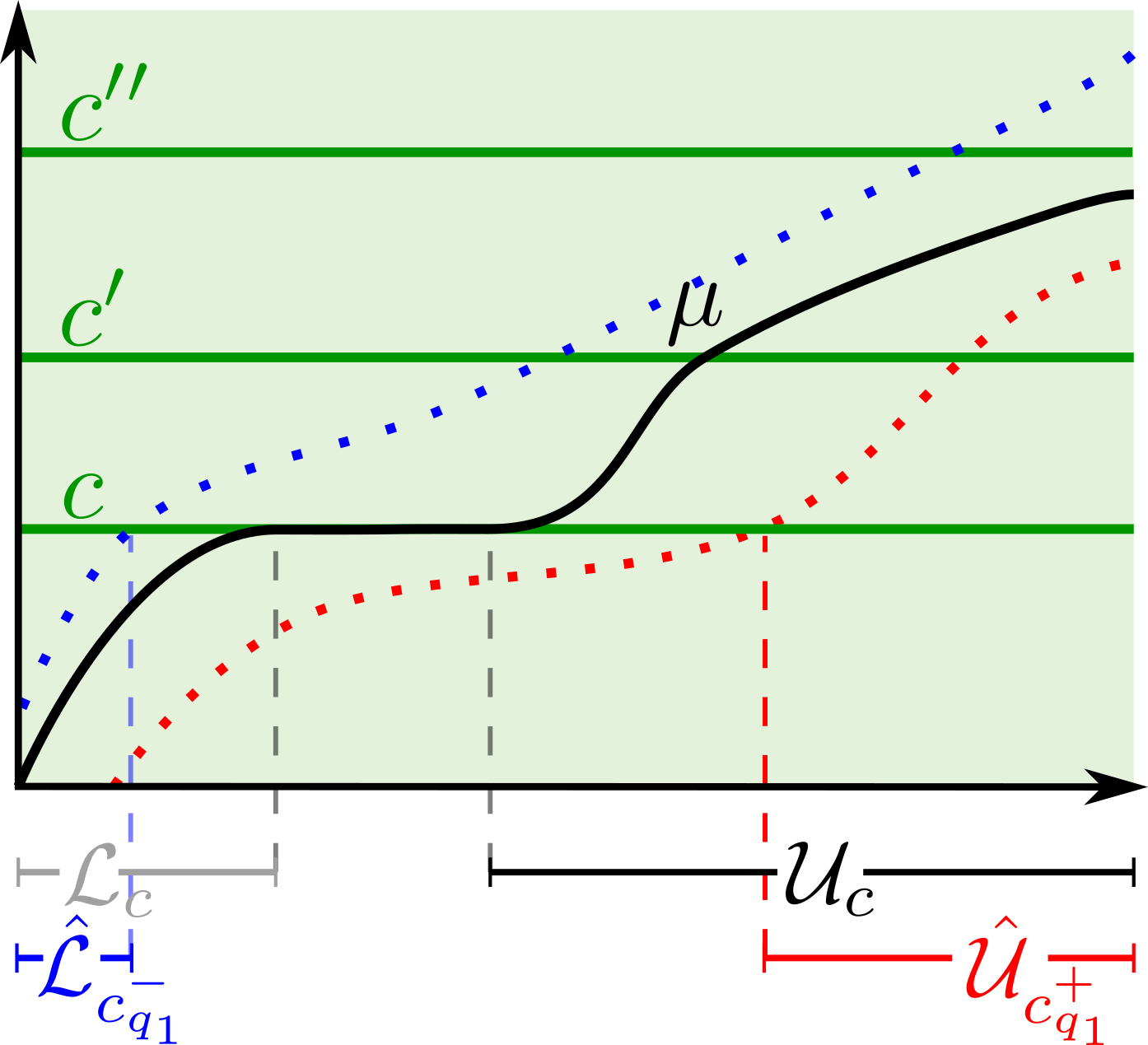
Figure 1: Illustration of three different inference questions on a real-valued function $\mu$. The blue dotted line is $\hat{\mu}_{N}+\tau_{N}q_{i}\sigma$ and the red dotted line $\hat{\mu}_{N}-\tau_{N}q_{i}\sigma$ for $i=\{1,2,3\}$. Left: $q_{1}$ is the quantile of a $(1-\alpha)$-SCB. This means that $\hat{\mathcal{L}}_{\tilde{c}-\tau_{N}q_{\alpha}\sigma}\subseteq\mathcal{L}_{\tilde{c}}$ and $\hat{\mathcal{U}}_{\tilde{c}+\tau_{N}q_{\alpha}\sigma}\subseteq\mathcal{U}_{\tilde{c}}$ hold simultaneously for all $\tilde{c}\in\mathcal{F}(S)$. Middle: only lower and upper excursion sets above $\tilde{c}$ such that the graph of $\tilde{c}$ is contained in $S\times[c,c^{\prime}]$ are controlled simultaneously with probability $1-\alpha$ so that in general $q_{2}\leq q_{1}$. Here $\hat{\mathcal{U}}_{c^{\prime\prime}+\tau_{N}q_{\alpha}\sigma}\not\subseteq\mathcal{U}_{c^{\prime\prime}}$, yet for $c$ and $c^{\prime}$ all the inclusions hold. Right: only $\hat{\mathcal{L}}_{c-\tau_{N}q_{\alpha}\sigma}\subseteq\mathcal{L}_{c}$ and $\hat{\mathcal{U}}_{c+\tau_{N}q_{\alpha}\sigma}\subseteq\mathcal{U}_{c}$ are controlled and therefore in general $q_{3}\leq q_{2}$. This is the target of statistical hypothesis tests of the alternatives $\mathbf{H}_{0,s}:~{}\mu(s)=c$ vs. $\mathbf{H}_{1,s}:~{}\mu(s)\neq c$.

1.2 An Asymptotic SCoPE Sets Theorem

In our main theorem we construct asymptotic $(1-\alpha)$-SCoPE sets over $(\mathcal{C}^{-},\mathcal{C}^{+})$ from an estimator $\hat{\mu}_{N}$ of $\mu$. In order to circumvent problems of measurability, we work in the J. Hoffmann-Jørgensen framework of weak convergence [50, Chapter 1-3]. Our main assumption is slightly stronger than that the restriction of the estimator $\hat{\mu}_{N}$, $N\in\mathbb{N}$, to a set $U\subseteq S$ which is specified later satisfies a uniform limit theorem (ULT) in $\ell^{\infty}(U)$. This means that there exists a strictly positive sequence $(\tau_{N})_{N\in\mathbb{N}}$ converging to zero (the inverse of the usual rate) and a positive function $\sigma\in\ell^{\infty}(U)$ such that $\frac{\hat{\mu}_{N}-\mu}{\tau_{N}\sigma}$ converges weakly in $\ell^{\infty}(U)$ to a tight limiting process $G$ with sample paths in $\ell^{\infty}(U)$. If we define the preimages of $\mu$ under the sets $\mathcal{C}^{\pm}$ to be $\mu^{-1}_{\mathcal{C}^{\pm}}=\big{\{}\,s\in S~{}|~{}\exists c\in\mathcal{C}^{\pm}:~{}\mu(s)=c(s)\,\big{\}}$ then our main result Theorem 1 –up to technical details– has the form

$$\begin{split}\lim_{N\rightarrow\infty}\mathbb{P}\Bigg{[}~{}\forall c^{-}\in\mathcal{C}^{-}\forall c^{+}\in\mathcal{C}^{+}:~{}&\hat{\mathcal{L}}_{c_{q}^{-}}\subseteq\mathcal{L}_{c^{-}}~{}\wedge~{}\hat{\mathcal{U}}_{c_{q}^{+}}\subseteq\mathcal{U}_{c^{+}}~{}\Bigg{]}\\ &=\mathbb{P}\left[\max\left(\sup_{s\in\mu^{-1}_{\mathcal{C}^{-}}}-G(s),\sup_{s\in\mu^{-1}_{\mathcal{C}^{+}}}G(s)\right)<q\right]\,.\end{split}$$ (1)

The proof is surprisingly simple and similar to the proofs of the main results in [27] and [43]. It consists of first showing that the r.h.s. is a lower bound of the $\liminf$ of the l.h.s. of (1). This is established using Lemma 2 which provides algebraic sufficient conditions so that $\hat{\mathcal{L}}_{c_{q}^{-}}\subseteq\mathcal{L}_{c^{-}}$ and $\hat{\mathcal{U}}_{c_{q}^{-}}\subseteq\mathcal{U}_{c^{-}}$ based on suprema of $G_{N}=\frac{\hat{\mu}_{N}-\mu}{\tau_{N}\sigma}$ over certain sets $U_{N}^{\pm}$ and $S\setminus U_{N}^{\pm}$. Since the sets $U_{N}^{\pm}$ converge in Hausdorff distance to the set $\mu^{-1}_{\mathcal{C}^{\pm}}$ the $\max$-$\sup$ expression with $G$ replaced by $G_{N}$ and $\mu^{-1}_{\mathcal{C}^{\pm}}$ replaced by $U_{N}^{\pm}$ converges weakly to the $\max$-$\sup$ expression of $G$ on the r.h.s. of (1) under continuity assumptions on $G_{N}$ which are detailed in Section 4. The lower bound then follows using asymptotically tightness properties on an error process defined on $S\setminus\big{(}U_{N}^{-}\cup U_{N}^{+}\big{)}$ and an application of the Portmanteau Theorem. Similarly, the $\limsup$ of the l.h.s. can be bounded from above by the r.h.s. based on simple algebra and the Portmanteau Theorem applied to the random variable where in the $\max$-$\sup$ expression on the r.h.s. $G$ is replaced by $G_{N}$. This proof technique is condensed and generalized in the SCoPE Set Metatheorem (Appendix B) which is the core of all our results.

Estimating $q$ such that the families $\big{\{}\hat{\mathcal{L}}_{c_{q}^{-}}\big{\}}_{c^{-}\in\mathcal{C}^{-}}$ and $\big{\{}\hat{\mathcal{U}}_{c_{q}^{+}}\big{\}}_{c^{+}\in\mathcal{C}^{+}}$ form asymptotic ${(1-\alpha)}$-SCoPE sets over $(\mathcal{C}^{-},\mathcal{C}^{+})$ requires estimation of the quantiles of the process on the r.h.s. of (1). In particular, the preimages $\mu^{-1}_{\mathcal{C}^{\pm}}$ – more precisely generalized preimages $\mathfrak{u}^{-1}_{\mathcal{C}^{\pm}}$ in the case that $\mu$ or the functions in $\mathcal{C}^{\pm}$ are discontinuous – must be estimated. In Section 4.3 a Hausdorff-distance consistent estimator of $\mathfrak{u}^{-1}_{\mathcal{C}^{\pm}}$ under the assumptions of our main theorem is discussed (see Theorem 2) and we sketch a general strategy based on the multiplier bootstrap, as used for example in [11], to consistently estimate the quantile $q$. Concrete estimation of $q$, however, depends on the particular probabilistic model.

In this work we focus on properties deducible from general assumptions on the estimator $\hat{\mu}_{N}$ of $\mu$. Nevertheless we demonstrate in Appendix 5.4 that Theorem 1 can be used to construct a strong $\alpha$-FWER test for iid observations which in this scenario is more powerful than Hommel’s procedure [22]. Here we also introduce the concept of insignificance values to post-hoc judge the validity of SCoPE sets. Moreover, our Section 6 on connections between SCoPE sets and multiple tests and the upcoming literature review will reveal that among others, the inference strategies from [43, 5, 6, 11, 9, 10, 13] can be viewed as applications of Theorem 1 which indicates its broad applicability.

1.3 SCoPE sets and Hypothesis Testing

A possible interpretation of Theorem 1 is that the r.h.s. of (1) which depends on the unknown function $\mu$ characterizes oracle limiting distributions for different asymptotic strong $\alpha$-FWER tests. From the perspective of multiple hypothesis testing each statement of the form $\hat{\mathcal{L}}_{c_{q_{\alpha}}^{-}}\subseteq\mathcal{L}_{c^{-}}$ suggests a test on $\mathbf{H}_{0,s}:\mu(s)<c(s)$ versus $\mathbf{H}_{1,s}:\mu(s)\geq c(s)$ by accepting $\mathbf{H}_{0,s}$ if $s\in\hat{\mathcal{L}}_{c_{q_{\alpha}}^{-}}$ and rejecting it otherwise. If $q_{\alpha}$ corresponds to $(1-\alpha)$-SCoPE sets over $(\mathcal{C}^{-},\mathcal{C}^{+})$ with $c^{-}\in\mathcal{C}^{-}$ then this test controls the FWER at level $\alpha$ because $\mathbb{P}\big{[}\hat{\mathcal{L}}_{c_{q_{\alpha}}^{-}}\not\subseteq\mathcal{L}_{c}\big{]}=1-\mathbb{P}\big{[}\hat{\mathcal{L}}_{c_{q_{\alpha}}^{-}}\subseteq\mathcal{L}_{c}\big{]}\leq\alpha$ and $\mathcal{L}_{c^{-}}$ is the set of true null hypotheses. This interpretation allows to construct strong $\alpha$-FWER tests based on SCoPE sets for complex hypotheses.

For $b_{\pm}\in\mathcal{F}(S)$ such that $b_{-}(s)\leq b_{+}(s)$ for all $s\in S$, a local Relevance Test is a multiple hypothesis test on the hypotheses

$$\begin{split}\mathbf{H}^{rel}_{0,s}\mathbf{:}~{}~{}\mu(s)\in\big{[}b_{-}(s),b_{+}(s)\big{]}~{}~{}~{}\text{vs.}~{}~{}~{}\mathbf{H}^{rel}_{1,s}\mathbf{:}~{}~{}\mu(s)\notin\big{[}b_{-}(s),b_{+}(s)\big{]}\end{split}$$

for all $s\in S$. In Section 6.1 we construct a local relevance test based on SCoPE sets which asymptotically controls the FWER over $S$ in the strong sense (Theorem 4). To the best of our knowledge no such test has been proposed yet. Only tests on the global hypothesis $\mu(s)\in\big{[}b_{-}(s),b_{+}(s)\big{]}$ for all $s\in S$ have been discussed in the literature. Examples with $b_{\pm}(s)=\pm\Delta$ for all $s\in S$ are the test on having somewhere a relevant difference between the population means and for having somewhere a relevant difference between the covariance operators for two samples of $C\big{(}[0,1]\big{)}$-valued random variables from [11] and [10] respectively. This strategy was recently extended to function-on-function regression [13]. Our Theorem 3 generalizes the test strategy of the aforementioned articles and shows that these tests are based on SCoPE sets. In consequence Theorem 3 explains that the validity of their testing strategy follows immediately from a ULT of the considered estimator $\hat{\mu}_{N}$ of their target function $\mu$ which is always the first step in their proofs. Hence even our local relevance test from Theorem 4 can be applied to the probabilistic models and estimators discussed in [11, 10, 13]. The generalizations which Theorem 3 grants are a strategy to adapt the test-statistic to the asymptotic variance of $\hat{\mu}_{N}$ or any other scaling function, allowing $b_{\pm}$, $\mu$ and $\hat{\mu}_{N}$ to be discontinuous and showing that $S$ can be an arbitrary metric space.

Similarly, we derive from Theorem 1 a test in Section 6.2 for the hypothesis

$$\begin{split}\mathbf{H}^{eqv}_{0}\mathbf{:}~{}~{}\exists s\in S:~{}\mu(s)\notin\big{[}b_{-}(s),b_{+}(s)\big{]}\,~{}~{}~{}\text{vs.}~{}~{}~{}\mathbf{H}^{eqv}_{1}\mathbf{:}~{}~{}\forall s\in S:~{}\mu(s)\in\big{[}b_{-}(s),b_{+}(s)\big{]}\,.\end{split}$$

Such equivalence tests have been studied, among others, for multivariate data ($S$ discrete and finite) [53, Chapter 7.3] and [51], for regression curves [12, 31] and in the cases of the difference of two mean functions or the quotient of two variance functions in functional data in [15] and [9]. As in the case of the local relevance test our Theorem 5 generalizes the testing strategy of these articles and embeds it into the SCoPE sets framework.

Last but not least, we derive in Section 6.3 a local Equivalence Test based on SCoPE sets. It is a multiple hypothesis test on the alternatives

$$\begin{split}\mathbf{H}^{leqv}_{0,s}\mathbf{:}~{}~{}\mu(s)\notin\big{[}b_{-}(s),b_{+}(s)\big{]}~{}~{}~{}\text{vs.}~{}~{}~{}\mathbf{H}^{leqv}_{1,s}\mathbf{:}~{}~{}\mu(s)\in\big{[}b_{-}(s),b_{+}(s)\big{]}\,.\end{split}$$

Since the role of the null and alternative hypothesis is interchanged compared to local relevance tests it is not surprising that Theorem 6 establishes that our local equivalence test based on SCoPE sets has similar properties as our local relevance test, for example, being a strong $\alpha$-FWER test. We could not find any previous work on such tests. An application could be detecting which drugs are equivalent in an experiment where several drug-treatment comparisons (indexed by $s$) have been recorded.

1.4 Connections to the Literature

The first work we are aware of which quantifies the uncertainty of the lower and the upper excursion set above zero of a function $\mu$ defined on $\mathbb{R}^{D}$ is [27]. Using an estimator $\hat{\mu}_{N}$ of $\mu$ it constructs a lower and an upper excursion set $\hat{\mathcal{L}}$ and $\hat{\mathcal{U}}$ respectively such that both inclusions $\hat{\mathcal{L}}\subseteq\mathcal{L}_{0}$ and $\hat{\mathcal{U}}\subseteq\mathcal{U}_{0}$ hold asymptotically with a prespecified probability. They apply these sets to quantify the uncertainty of the excursion sets of a kernel density estimator above a single $c\in\mathbb{R}$, but do not explicitly extract the asymptotic distribution. However, they even derive a non-asymptotic bound [27, Lemma 2.1.] which can also be derived from our Proposition 2 from Appendix B.

Another recent work on confidence sets for a single level or upper excursion set of an unknown density using kernel density estimators is [33]. In particular they derive assumptions and rates for having asymptotically nominal coverage. We recommend it also for its broad overview on applications of level and excursion set estimation.

Assuming that $S\subset\mathbb{R}^{D}$ is compact, $c\in\mathbb{R}$ and $\hat{\mu}_{N}$ satisfies a uniform central limit theorem, [43] finds the limit distribution of the inclusions $S\setminus\hat{\mathcal{L}}_{c^{+}_{q}}\subseteq S\setminus\mathcal{L}_{c}\subseteq S\setminus\hat{\mathcal{L}}_{c^{-}_{q}}$. Although is seems reasonable at first to use only upper excursion sets with ”$\geq$”-signs, it has two shortcomings. First their limit result holds only under the assumption that $\mu$ is not flat on the level set $\{s\in S~{}|~{}\mu(s)=c\}$ [43, Assumption 2.1.(a) and Lemma 1]. Hence their result cannot be connected to testing. Second, their inclusion statement does not provide a random partition of $S$ while $(1-\alpha)$-SCoPE sets over $\big{(}\{c\},\{c\}\big{)}$ give a random partition of $S$ into three sets, i.e.,

$$\hat{\mathcal{L}}_{c_{q}^{-}}\subseteq\mu^{-1}[-\infty,c)\,,~{}~{}S\setminus\big{(}\hat{\mathcal{L}}_{c_{q}^{-}}\cup\hat{\mathcal{U}}_{c_{q}^{+}}\big{)}\supseteq\mu^{-1}(c)\,,~{}~{}\hat{\mathcal{U}}_{c_{q}^{+}}\subseteq\mu^{-1}(c,\infty)\,,$$ (2)

for which all inclusions hold (asymptotically) simultaneously with a probability depending on $q$. In other words, this partition consists of asymptotic $(1-\alpha)$-confidence subsets for $\mathcal{L}_{c}$ and $\mathcal{U}_{c}$ and a $(1-\alpha)$-confidence superset for $\mu^{-1}(c)$. The inclusion from [43] only yields

$$\hat{\mathcal{L}}_{c_{q}^{-}}\subseteq\mu^{-1}[-\infty,c)\,,~{}~{}S\setminus\hat{\mathcal{L}}_{c^{+}_{q}}\subseteq\mu^{-1}[c,\infty)\,.$$

A superset for $\mu^{-1}(c)$ cannot be directly obtained from their main result [43, Corollary 1]. These problems persist in the applications of this work to geoscience [16] and neuroimaging [5, 6] and the innovative work [29]. The latter generalizes [43] to intersections and unions of excursion sets of several functions $\mu^{1},\ldots,\mu^{K}$, $K\in\mathbb{N}$, above a single $c\in\mathbb{R}$. Our Corollary 3 generalizes the main theorem from [43]. It allows $S$ to be an arbitrary metric space, requires weaker assumptions and provides a partition of $S$ of the form (2).

To date only [34] is dealing with several excursion sets at the same time. Their main theorem shows that properly thresholding SCBs yields simultaneous confidence sets for all lower and upper excursion sets over $c\in\mathbb{R}$. We generalize their main result in our Proposition 1 by showing that the control is even simultaneous over all $c\in\mathcal{F}(S)$.

Our Corollary 1 connects asymptotic $(1-\alpha)$-SCBs (among others, [8, 47]) with $(1-\alpha)$-SCoPE sets over $\big{(}\mathcal{F}(S),\mathcal{F}(S)\big{)}$. Unsurprisingly, the fast and fair SCBs [25] can be used to generate $(1-\alpha)$-SCoPE sets over $\big{(}\mathcal{F}(S),\mathcal{F}(S)\big{)}$, too. Deriving this result requires the SCoPE Set Metatheorem since their key innovation is that the quantile parameter $q$ is a function which is chosen such that the invalidation of the coverage is fairly spread over a partition of $S=[0,1]$. We do not include this result here, since we restrict ourselves to constant $q$.

Recently, relevance tests [11, 13, 10] and equivalence tests [9, 12] in the space of continuous functions over $S=[0,1]$ have been studied. These articles focus on using $\|\hat{\mu}_{N}\|_{\infty}=\sup_{s\in S}|\hat{\mu}_{N}(s)|$ as the test statistic and derive limiting distributions depending on the set of extreme points of $\mu$ under the null and alternative hypothesis. Due to the focus on the supremum norm these tests cannot identify $s\in S$ such that the considered hypothesis is invalidated. As explained earlier in detail, our Theorems 4 and 6 go a step further and provide strong $\alpha$-FWER relevance and equivalence tests and therefore grant probabilistic bounds that all rejected $s\in S$ are points at which the considered null hypothesis is correctly rejected.

1.5 Organization of the Article

In Section 2 we introduce notations and definitions required to understand our main results. In Section 3 we rigorously define SCoPE sets and provide the link between $(1-\alpha)$-SCBs and $(1-\alpha)$-SCoPE sets over $\big{(}\mathcal{F}(S),\mathcal{F}(S)\big{)}$. Our main result (Theorem 1) and the required assumptions are discussed in Section 4. It also contains a general strategy to consistently estimate generalized preimages and provides a pathway to estimate the quantile parameter $q$. Section 5 gives a short glance into applications of SCoPE sets such as providing simultaneous control over regions of interest, confidence regions of several contour lines or detection of contrasts in multiple linear regression. Connections between SCoPE sets and statistical hypothesis testing are explored in Section 6 and in Section 7 we discuss observations and consequences of the introduced methodology.

2 Notations and Definitions

In this article $(S,d)$ denotes a metric space. $S\setminus B$, ${\rm cl}B$ for the topological closure, ${\rm int}B$ for the interior and $\partial B={\rm cl}B\setminus{\rm int}B$ for the topological boundary of $B$. The set $\mathcal{F}(S)$ denotes the set of functions $f:S\rightarrow\mathbb{R}\cup\{\pm\infty\}$. The set $\ell^{\infty}(S)\subset\mathcal{F}(S)$ is the set of all bounded functions $f\in\mathcal{F}(S)$, i.e., $\|f\|_{\infty}=\sup_{s\in S}|f(s)|<\infty$ and $C(S)\subseteq\mathcal{F}(S)$ is the subset of continuous functions with respect to the topology generated by the metric $d$. If $f\in\mathcal{F}(S)$ and $r\in\mathbb{R}\cup\{\pm\infty\}$, we write $f\equiv r$, if $f$ is the constant function with value $r$ and if no confusion is possible we identify $r$ with the constant function with value $r$. For any $f\in\mathcal{F}(S)$ we define, as usual,

$$\sup_{s\in\emptyset}f(s)=-\infty~{}~{}\text{ and }~{}~{}\inf_{s\in\emptyset}f(s)=\infty\,.$$ (3)

Let $(\Omega,\mathfrak{P},\mathbb{P})$ be a probability space. Our theory is based on the J. Hoffmann-Jørgensen theory of weak convergence. Thus, recall that the inner probability of a set $V\subset\Omega$ is given by $\mathbb{P}_{*}(V)=\sup\{\,\mathbb{P}(W)~{}|~{}W\subseteq V\,,W\in\mathfrak{P}\,\}$, and its outer probability by $\mathbb{P}^{*}(V)=\inf\{\,\mathbb{P}(W)~{}|~{}W\supseteq V\,,W\in\mathfrak{P}\,\}$. Because we will repeatedly use the statements $(i)$ and $(ii)$ of the Portmanteau Theorem [50, Theorem 1.3.4], we introduce the following notation.

Definition 1.

Let $\Omega_{N}\subset\Omega$ be a sequence of sets, $X:\Omega\rightarrow\mathbb{R}$ a random variable and $q\in\mathbb{R}$. We write $\lim_{N\rightarrow\infty}\mathbb{P}_{*}\big{[}\Omega_{N}\big{]}=\mathbb{P}\big{[}X\prec q\big{]}$ under Assumptions (A) / (B) if the following two statements hold:

$$\begin{split}&\text{Under Assumptions {\rm{(A)}}}:~{}~{}~{}\liminf_{N\rightarrow\infty}\mathbb{P}_{*}\big{[}\Omega_{N}\big{]}\geq\mathbb{P}\big{[}X<q\big{]}\\ &\text{Under Assumptions {\rm{(B)}}}:~{}~{}~{}\limsup_{N\rightarrow\infty}\mathbb{P}^{*}\big{[}\Omega_{N}\big{]}\leq\mathbb{P}\big{[}X\leq q\big{]}.\end{split}$$

Our asymptotic theory of SCoPE sets is developed in terms of preimages and graphs of functions. Therefore we extend these concepts to (possible uncountable) sets $\mathcal{F}\subseteq\mathcal{F}(S)$. Recall that the graph of $f\in\mathcal{F}(S)$ is the set $\Gamma(f)=\big{\{}~{}(s,r)\in S\times\mathbb{R}~{}|~{}r=f(s)~{}\big{\}}\,.$

Definition 2 (Graph of a Set of Functions).

For $\mathcal{F}\subseteq\mathcal{F}(S)$ we define the graph of $\mathcal{F}$ to be the set $\Gamma(\mathcal{F})=\bigcup_{f\in\mathcal{F}}\Gamma(f)$ and we write $f\in\Gamma(\mathcal{F})$ if $\Gamma(f)\subseteq\Gamma(\mathcal{F})$ for $f\in\mathcal{F}(S)$.

Definition 3 (Preimage of a Set of Functions).

For $\mathcal{F}\subseteq\mathcal{F}(S)$ and $\mu\in\mathcal{F}(S)$ we define the $\mathcal{F}$-preimage under $\mu$ by $\mu^{-1}_{\mathcal{F}}=\mu^{-1}(\mathcal{F})=\big{\{}\,s\in S~{}|~{}\exists f\in\mathcal{F}:~{}f(s)=\mu(s)\,\big{\}}\,.$ If $\mathcal{F}=\{f\}$, $f\in\mathcal{F}(S)$, the abbreviation $\mu^{-1}_{\{f\}}=\mu^{-1}_{f}$ is used.

If $\mathcal{F}\not\subset\mathcal{C}(S)$ or $\mu\notin\mathcal{C}(S)$ we need to generalize the concept of a preimage of a set of functions in order to add all “touching points” of $\Gamma(\mu)$ and $\Gamma(\mathcal{F})$ to the preimage. To make this idea mathematically precise we first introduce thickenings of the set $\mathcal{F}$.

Definition 4 (Thickenings of a Set of Functions).

For $\mathcal{F}\subseteq\mathcal{F}(S)$ and $\eta>0$ the set $\mathcal{F}_{\pm\eta}=\big{\{}\,f\pm\varepsilon\in\mathcal{F}(S)~{}|~{}f\in\mathcal{F},~{}0\leq\varepsilon\leq\eta\,\big{\}}$ is called $\pm\eta$-thickening of $\mathcal{F}$. The set $\mathcal{F}_{\eta}=\mathcal{F}_{-\eta}\cup\mathcal{F}_{+\eta}$ will be called the $\eta$-thickening of $\mathcal{F}$.

Definition 5 (Generalized Preimages of a Set of Functions).

For $\mathcal{F}\subseteq\mathcal{F}(S)$ and $\mu\in\mathcal{F}(S)$ the generalized upper(+)/lower(-) preimage of $\mathcal{F}$ under $\mu$ is the set $\mathfrak{u}^{-1}_{\pm\mathcal{F}}=\bigcap_{\eta>0}{\rm cl}\,\mu^{-1}_{\mathcal{F}_{\pm\eta}}\,.$ The generalized preimage is $\mathfrak{u}^{-1}_{\mathcal{F}}=\mathfrak{u}^{-1}_{-\mathcal{F}}\cup\mathfrak{u}^{-1}_{+\mathcal{F}}$.

Obviously, $\mu^{-1}_{\mathcal{F}},\mu^{-1}_{\pm\mathcal{F}}\subseteq\mathfrak{u}^{-1}_{\mathcal{F}}$ which explains the name generalized preimages. Its importance for us lies in the observation that, if ${\rm cl}\mu^{-1}_{\pm\mathcal{F}_{\eta}}$ is compact for some $\eta>0$ and $\mathfrak{u}^{-1}_{\mathcal{F}}\neq\emptyset$, it holds that

$$\lim_{N\rightarrow\infty}d_{H}\Big{(}{\rm cl}\,\mu^{-1}_{\mathcal{F}_{\pm\eta_{N}}},\mathfrak{u}^{-1}_{\pm\mathcal{F}}\Big{)}=0$$ (4)

for any positive sequence $(\eta_{N})_{N\in\mathbb{N}}\subset\mathbb{R}$ converging to zero [49, Corollary 5.30] and $\mathfrak{u}^{-1}_{\pm\mathcal{F}}$ is the unique closed set with this property. If there would be another $A\subseteq S$ satisfying (4), it holds by the triangle inequality that

$$d_{H}\left(\mathfrak{u}^{-1}_{\pm\mathcal{F}},A\right)\leq\lim_{N\rightarrow 0}d_{H}\left({\rm cl}\,\mu^{-1}_{\pm\mathcal{F}_{\eta_{N}}},\mathfrak{u}^{-1}_{\mathcal{F}}\right)+d_{H}\left({\rm cl}\,\mu^{-1}_{\pm\mathcal{F}_{\eta_{N}}},A\right)=0$$

and therefore $\mathfrak{u}^{-1}_{\pm\mathcal{F}}={\rm cl}A$ [49, Problem 5.1.(3)].

All our results have a similar limit distribution. Therefore we introduce the following two notations for $\mathcal{F},\mathcal{G}\subseteq\mathcal{F}(S)$ and $f$ a real-valued function with appropriate domain:

$$\begin{split}T_{\mathcal{F},\mathcal{G}}(f)&=\max\Bigg{(}\sup_{s\in{\rm cl}\,\mu^{-1}_{\mathcal{F}}}-f(s),~{}\sup_{s\in{\rm cl}\,\mu^{-1}_{\mathcal{G}}}f(s)\Bigg{)}\\ \mathfrak{T}_{\mathcal{F},\mathcal{G}}(f)&=\max\Bigg{(}\sup_{s\in\mathfrak{u}^{-1}_{+\mathcal{F}}}-f(s),~{}\sup_{s\in\mathfrak{u}^{-1}_{-\mathcal{G}}}f(s)\Bigg{)}\,.\end{split}$$ (5)

We also write $T_{\mathcal{F},\mathcal{F}}(f)=T_{\mathcal{F}}(f)$ and $\mathfrak{T}_{\mathcal{F},\mathcal{F}}(f)=\mathfrak{T}_{\mathcal{F}}(f)$.

3 Simultaneous Coverage Probability Excursion Sets

As explained in the introduction our main interest is providing inference strategies on level sets of a function $\mu$ given a function $\hat{\mu}_{N}:~{}\Omega\rightarrow\mathcal{F}(S)$, $N\in\mathbb{N}$, obtained from data. We call $\hat{\mu}_{N}$ an estimator of $\mu$, yet we do not require that it is measurable.

Definition 6.

Let $f\in\mathcal{F}(S)$. The lower and upper excursion sets of $\mu$ over $f$ are $\mathcal{L}_{f}(\mu)=\mathcal{L}_{f}=\big{\{}\,s\in S~{}|~{}\mu(s)<f(s)\,\big{\}}$ and $\mathcal{U}_{f}(\mu)=\mathcal{U}_{f}=\big{\{}\,s\in S~{}|~{}\mu(s)>f(s)\,\big{\}}$, respectively. For an estimator $\hat{\mu}_{N}$ we define the (random) sets $\mathcal{L}_{f}(\hat{\mu}_{N})=\hat{\mathcal{L}}_{f}$ and $\mathcal{U}_{f}(\hat{\mu}_{N})=\hat{\mathcal{U}}_{f}$.

Definition 7.

Let $\alpha\in(0,1)$, $\mathcal{C}^{\pm}\subseteq\mathcal{F}(S)$ and $c^{\pm}_{\alpha}\in\mathcal{F}(S)$ correspond to a $c^{\pm}\in\mathcal{C}^{\pm}$. Then the two families of set-valued functions $\big{\{}\hat{\mathcal{L}}_{c^{-}_{\alpha}}\big{\}}_{c^{-}\in\mathcal{C^{-}}}$ and $\big{\{}\hat{\mathcal{U}}_{c^{+}_{\alpha}}\big{\}}_{c^{+}\in\mathcal{C^{+}}}$ such that

$$\begin{split}\Big{(}\liminf_{N\rightarrow\infty}\Big{)}\mathbb{P}_{*}\left[~{}\forall c^{-}\in\mathcal{C}^{-}\,\forall c^{+}\in\mathcal{C}^{+}:~{}\hat{\mathcal{L}}_{c^{-}_{\alpha}}\subseteq\mathcal{L}_{c^{-}}~{}\wedge~{}\hat{\mathcal{U}}_{c^{+}_{\alpha}}\subseteq\mathcal{U}_{c^{+}}\,\right]\geq{1-\alpha}\end{split}$$

are called (asymptotic) ${(1-\alpha)}$-SCoPE sets over $(\mathcal{C}^{-},\mathcal{C}^{+})$. We call them exact, if additionally

$$\begin{split}\Big{(}\limsup_{N\rightarrow\infty}\Big{)}\mathbb{P}^{*}\left[~{}\forall c^{-}\in\mathcal{C}^{-}\,\forall c^{+}\in\mathcal{C}^{+}:~{}\hat{\mathcal{L}}_{c^{-}_{\alpha}}\subseteq\mathcal{L}_{c^{-}}~{}\wedge~{}\hat{\mathcal{U}}_{c^{+}_{\alpha}}\subseteq\mathcal{U}_{c^{+}}\,\right]\leq{1-\alpha}\,.\end{split}$$

Remark 1.

Our definition involves outer and inner probabilities, since even if $\hat{\mu}_{N}$ is measurable it depends on the probabilistic model whether the union of the inclusion statements is measurable, especially if $\mathcal{C}^{-}$ or $\mathcal{C}^{+}$ is uncountable.

If $\mathbb{R}$ is identified with the constant functions, then the main result from [34] can be viewed as the first result on non-asymptotic $(1-\alpha)$-SCoPE sets over $(\mathbb{R},\mathbb{R})$. It shows that any $(1-\alpha)$-SCB for a function $\mu$ allows to construct $(1-\alpha)$-SCoPE sets over $(\mathbb{R},\mathbb{R})$. Our next proposition generalizes this result because it shows that $\mathbb{R}$ can be replaced by $\mathcal{F}(S)$. To stay within our notation we only discuss $(1-\alpha)$-SCBs of the form $\big{[}\,\hat{\mu}_{N}(s)-q\tau_{N}\hat{\sigma}_{N}(s),\hat{\mu}_{N}(s)+q\tau_{N}\hat{\sigma}_{N}(s)\,\big{]}$. The general case of $(1-\alpha)$-SCBs of the form $\big{[}\,\hat{l}(s),\hat{u}(s)\,\big{]}$, $s\in S$, where $\hat{u},\hat{l}\in\mathcal{F}(S)$ with $\hat{l}(s)<\hat{u}(s)$ can be treated analogously. It only requires to assume that the event $\big{\{}\omega\in\Omega~{}|~{}\forall s\in S:~{}\mu(s)\geq\hat{l}(s)\big{\}}$ and $\big{\{}\omega\in\Omega~{}|~{}\forall s\in S:~{}\mu(s)\leq\hat{u}(s)\big{\}}$ are measurable.

Proposition 1.

Let $S$ be separable, $\mu\in\mathcal{F}(S)$, $\tau_{N}>0$, $\hat{\mu}$ be a $\mathbb{R}$-valued and $\hat{\sigma}$ a $\mathbb{R}_{>0}$-valued stochastic process and assume that the process $\frac{\hat{\mu}(s)-\mu(s)}{\tau_{N}\hat{\sigma}(s)}$ is separable. Then

$$\begin{split}\mathbb{P}\Big{[}\,\forall c^{-},c^{+}\in\mathcal{F}(S):~{}\hat{\mathcal{L}}_{c^{-}-q\tau_{N}\hat{\sigma}}\subseteq\mathcal{L}_{c^{-}}~{}\wedge~{}&\hat{\mathcal{U}}_{c^{+}+q\tau_{N}\hat{\sigma}}\subseteq\mathcal{U}_{c^{+}}\,\Big{]}\\ &=\mathbb{P}\left[\,\sup_{s\in S}\left|\frac{\hat{\mu}(s)-\mu(s)}{\tau_{N}\hat{\sigma}(s)}\right|\leq q\,\right]\,.\end{split}$$

Remark 2.

The proof of the above result establishes equality between sets. Thus, the measurability assumptions implicit in imposing that $\hat{\mu}$ and $\hat{\sigma}$ are stochastic processes and the separability can be removed, if the probabilities are replaced by outer or inner probabilities.

4 An Asymptotic SCoPE Sets Theorem

4.1 Assumptions

Hereafter we assume $\mu\in\ell^{\infty}(S)$ and $(\hat{\mu}_{N})_{N\in\mathbb{N}}$ is a sequence of estimators of $\mu$, i.e., $\hat{\mu}_{N}:\Omega\rightarrow\ell^{\infty}(S)$, $\sigma\in\ell^{\infty}(S)$ satisfies $0<\mathfrak{o}<\sigma(s)<\mathfrak{O}<\infty$ for all $s\in S$ and $(\tau_{N})_{N\in\mathbb{N}}\subset\mathbb{R}$ is a positive sequence converging to zero. Furthermore, we define a sequence $(G_{N})_{N\in\mathbb{N}}$ by

$$G_{N}=\frac{\hat{\mu}_{N}-\mu}{\tau_{N}\sigma}\,.$$ (6)

Definition 8.

For $\mathcal{C}\subseteq\mathcal{F}(S)$, an estimator $\hat{\mu}_{N}$ of $\mu$ with values in $\ell^{\infty}(S)$ is said to fulfill a uniform limit theorem on $\mathcal{C}_{\tilde{\eta}}$ (short $\mathcal{C}_{\tilde{\eta}}$-ULT) if the following conditions hold:

1. There is a tight, Borel measurable $G:\Omega\rightarrow\ell^{\infty}\big{(}{\rm cl}\,\mu^{-1}_{\mathcal{C}_{\tilde{\eta}}}\big{)}$ such that $G_{N}\rightsquigarrow G$ weakly in $\ell^{\infty}\big{(}{\rm cl}\,\mu^{-1}_{\mathcal{C}_{\tilde{\eta}}}\big{)}$ in the sense of [50, Definition 1.3.3].

2. There is a $K>0$ such that for every $s\in S\setminus\mu^{-1}_{\mathcal{C}_{\tilde{\eta}}}$ it holds almost surely (a.s.) that

   $$\big{(}\,\hat{\mu}_{N}(s)-c(s)\,\big{)}\cdot{\rm sgn}\big{(}\,\mu(s)-c(s)\,\big{)}\geq\sigma(s)\big{(}\,K+Z_{N}(s)\,\big{)}$$ (7)

   for all $c\in\mathcal{C}$ and $Z_{N}$ being a sequence of functions $\Omega\rightarrow\ell^{\infty}(S)$ such that $\inf_{s\in S}\tau_{N}^{-1}Z_{N}(s)$ is asymptotically tight in the sense of [50, p.21].

Remark 3.

At first, the second condition might appear abstract, yet it only means that $\hat{\mu}_{N}(s)-c(s)$ and $\mu(s)-c(s)$ for all $c\in\mathcal{C}$ have with probability tending to one the same sign for all $s\in S$ sufficiently far away from the generalized preimage $\mathfrak{u}^{-1}_{\mathcal{C}}$. This follows immediately from (7) and $\inf_{s\in S}\tau_{N}^{-1}Z_{N}(s)$ being asymptotically tight because

$$\begin{split}\limsup_{N\rightarrow\infty}&\,\mathbb{P}^{*}\Big{[}\,\exists s\in S\setminus\mu^{-1}_{\mathcal{C}_{\tilde{\eta}}}:~{}{\rm sgn}\big{(}\,\mu(s)-c(s)\,\big{)}=-{\rm sgn}\big{(}\,\hat{\mu}_{N}(s)-c(s)\,\big{)}\,\Big{]}\\ &\leq\limsup_{N\rightarrow\infty}\mathbb{P}_{*}\Big{[}\,\exists s\in S\setminus\mu^{-1}_{\mathcal{C}_{\tilde{\eta}}}:~{}-\big{|}\,\hat{\mu}_{N}(s)-c(s)\,\big{|}\geq\sigma(s)\big{(}\,K+Z_{N}(s)\,\big{)}\,\Big{]}\\ &\leq\limsup_{N\rightarrow\infty}\mathbb{P}^{*}\Big{[}\,\inf_{s\in S}Z_{N}(s)\leq-K\,\Big{]}\leq 1-\liminf_{N\rightarrow\infty}\mathbb{P}_{*}\Big{[}\,\inf_{s\in S}Z_{N}(s)\in[-K,K]\,\Big{]}=0\,.\end{split}$$

Remark 4.

To illustrate that the assumption of having a $\mathcal{C}_{\tilde{\eta}}$-ULT is not restrictive assume $\hat{\mu}_{N}=\mu+\sigma\tilde{Z}_{N}$. Then $\hat{\mu}_{N}$ satisfying a $\mathcal{C}_{\tilde{\eta}}$-ULT means that $\tau_{N}^{-1}\tilde{Z}_{N}\rightsquigarrow G$ on ${\rm cl}\,\mu^{-1}_{\mathcal{C}_{\tilde{\eta}}}$ and it holds for all $c\in\mathcal{C}$ and all $s\in S\setminus\mu^{-1}_{\mathcal{C}_{\tilde{\eta}}}$ that

$$\begin{split}\big{|}\,\mu(s)-c(s)\,\big{|}&+\sigma(s)\tilde{Z}_{N}(s)\cdot{\rm sgn}\big{(}\,\mu(s)-c(s)\,\big{)}\\ &\geq\sigma(s)\left(\inf_{s\in S\setminus\mu^{-1}_{\mathcal{C}_{\tilde{\eta}}}}\left\{\frac{\big{|}\,\mu(s)-c(s)\,\big{|}}{\sigma(s)}\right\}+\tilde{Z}_{N}(s)\cdot{\rm sgn}\big{(}\,\mu(s)-c(s)\,\big{)}\right)\\ &\geq\sigma(s)\left(K+\tilde{Z}_{N}(s)\cdot{\rm sgn}\big{(}\,\mu(s)-c(s)\,\big{)}\right)\,.\end{split}$$

Existence of $K>0$ follows from $\sigma(s)\leq\mathfrak{O}$ for $s\in S$ and $|\,\mu(s)-c(s)\,|>\tilde{\eta}$ for all $c\in\mathcal{C}$ on $S\setminus\mu^{-1}_{\mathcal{C}_{\tilde{\eta}}}$. The remaining requirement is that $\inf_{s\in S}\tau_{N}^{-1}\tilde{Z}_{N}(s)$ is asymptotically tight.

Given two sets $\mathcal{C}^{\pm}\subseteq\mathcal{F}(S)$ and $\tilde{\eta}>0$ we will need the following assumptions.

• The estimator $\hat{\mu}_{N}$ of $\mu$ satisfies a $\mathcal{C}_{\tilde{\eta}}$-ULT with $\mathcal{C}=\mathcal{C}^{-}\cup\mathcal{C}^{+}$.

• $G$ and $G_{N}$ from (A1) restricted to $\Big{(}{\rm cl}\,\mu^{-1}_{\mathcal{C}^{-}_{+\tilde{\eta}}}\setminus{\rm int}\,\mathfrak{u}^{-1}_{+\mathcal{C}^{-}}\Big{)}\cup\Big{(}{\rm cl}\,\mu^{-1}_{\mathcal{C}^{+}_{-\tilde{\eta}}}\setminus{\rm int}\,\mathfrak{u}^{-1}_{-\mathcal{C}^{+}}\Big{)}$ have a.s. continuous sample paths.

• If $\mathfrak{u}^{-1}_{\mp\mathcal{C}^{\pm}}\neq\emptyset$ and ${\rm cl}\,\mu^{-1}_{\mathcal{C}^{\pm}_{\mp\tilde{\eta}}}$ is not compact, then, for any positive sequence $(\eta_{N})_{N\in\mathbb{N}}$ converging to zero, $d_{H}\Big{(}{\rm cl}\,\mu^{-1}_{\mathcal{C}^{\pm}_{\mp\eta_{N}}},\mathfrak{u}^{-1}_{\mp\mathcal{C}}\Big{)}$ converges to zero as $N$ tends to infinity.

• Let $\mu^{-1}_{\mathcal{C}^{\pm}}=\mathfrak{u}^{-1}_{\mp\mathcal{C}^{\pm}}$ or let ${\rm cl}\,\mu^{-1}_{\mathcal{C}^{\pm}}=\mathfrak{u}^{-1}_{\mp\mathcal{C}^{\pm}}$ and there is an open $V^{\pm}\supset\partial\mu^{-1}_{\mathcal{C}^{\pm}}\setminus\mu^{-1}_{\mathcal{C}^{\pm}}$ such that $G_{N}(s)$ restricted to $V^{\pm}\cap\mu^{-1}_{\mathcal{C}^{\pm}}$ has a.s. continuous sample paths.

Remark 5.

If ${\rm cl}\,\mu^{-1}_{\mathcal{C}^{\pm}_{\mp\tilde{\eta}}}$ is compact (for example if $S$ is compact) then the Hausdorff convergence stated in Assumption (A3) is satisfied automatically, compare eq. (4). If ${\rm cl}\,\mu^{-1}_{\mathcal{C}^{\pm}_{\mp\tilde{\eta}}}$ is non-compact, then Assumption (A3) implies $\mathfrak{u}^{-1}_{\mp\mathcal{C}^{\pm}}\neq\emptyset$ because $\mathfrak{u}^{-1}_{\mp\mathcal{C}^{\pm}}=\emptyset$ yields

$$d_{H}\big{(}A,\mathfrak{u}^{-1}_{\mp\mathcal{C}^{\pm}}\big{)}=\sup_{s\in A}\inf_{s^{\prime}\in\emptyset}d(s,s^{\prime})=\infty$$

for all $A\subseteq S$ by convention (3) which explains the condition $\mathfrak{u}^{-1}_{\mp\mathcal{C}^{\pm}}=\emptyset$ in Assumption (A3).

The definition of $\mathfrak{u}^{-1}_{\mp\mathcal{C}^{\pm}}$ and Assumption (A3) might appear cryptic at a first glance. The important observation is that the Assumptions (A1)-(A3) imply

$$T_{\mathcal{C}_{+\eta_{N}}^{-},\mathcal{C}_{-\eta_{N}}^{+}}(G_{N})\rightsquigarrow\mathfrak{T}_{\mathcal{C}^{-},\mathcal{C}^{+}}(G)$$

weakly in $\mathbb{R}$ for any sequence $(\eta_{N})_{N\in\mathbb{N}}$ converging to zero. This is proven in Lemma 6 in Appendix A.3. The Hausdorff-convergence from (A3) is a crucial ingredient to prove this result which can fail if $\mu^{-1}_{\mathcal{C}^{\pm}}$ instead of the generalized preimage $\mathfrak{u}^{-1}_{\mp\mathcal{C}^{\pm}}$ are used (Fig. 2). If $S$ is compact, using $\mathfrak{u}^{-1}_{\mp\mathcal{C}^{\pm}}$ is only necessary if $\mu$ is not continuous or there is no set $\mathcal{C}^{\prime}\subseteq C(S)$ such that $\Gamma\big{(}\mathcal{C}\big{)}=\Gamma\big{(}\mathcal{C}^{\prime}\big{)}$ because otherwise it can be shown that $\mathfrak{u}^{-1}_{\mp\mathcal{C}^{\pm}}={\rm cl}\big{(}\mu^{-1}_{\mathcal{C}^{\pm}}\big{)}$ (Appendix C). Surprisingly, our proofs show that no continuity assumption on $\mu$ is necessary. We only need the continuity of $G$ and $G_{N}$ in neighborhood of $\mathfrak{u}^{-1}_{\mp\mathcal{C}^{\pm}}$ as stated in (A2) and (A4).

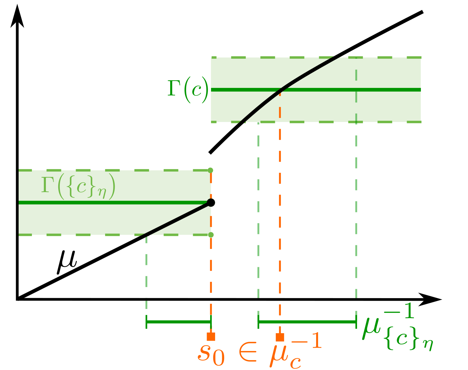
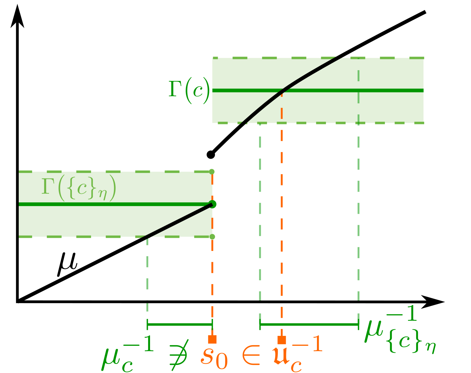
Figure 2: Illustration that $\mu^{-1}_{c}$ is not necessary the Hausdorff limit of ${\rm cl}\mu^{-1}_{\{c\}_{\eta}}$ as $\eta\rightarrow 0$. The problem are ”touching points” between $\Gamma(\mu)$ and $\Gamma(c)$ such as $s_{0}$ if $\mu$ or $c$ is discontinuous. Left: Since $c(s_{0})=\mu(s_{0})$ and $\mu$ restricted to ${\rm cl}\,\mu^{-1}_{\{c\}_{\tilde{\eta}}}\setminus{\rm int}\,\mu^{-1}_{c}$ is continuous it holds that $\mu^{-1}_{c}=\mathfrak{u}^{-1}_{c}$. Thus, $\mu^{-1}_{{\{c\}}_{\eta}}$ converges in Hausdorff distance to $\mu^{-1}_{c}$. Right: Since $\mu(s_{0})\neq c(s_{0})$ it holds that $s_{0}\notin\mu^{-1}_{c}$. Moreover, it is impossible that $\mu^{-1}_{c}$ is the Hausdorff limit of ${\rm cl}\mu^{-1}_{{\{c\}}_{\eta}}$ since for each $\eta>0$ there is an $s_{\eta}\in\mu^{-1}_{{\{c\}}_{\eta}}$ which is arbitrary close to $s_{0}$.

4.2 An Asymptotic SCoPE Sets Theorem

We can now state our main theorem about SCoPE sets which is a consequence of the more general SCoPE Set Metatheorem (Appendix B).

Theorem 1.

Let $\mathcal{C}^{\pm}\subseteq\mathcal{F}(S)$. Define $c_{q}^{\pm}=c^{\pm}\pm q\tau_{N}\sigma$ for all $c^{\pm}\in\mathcal{C}^{\pm}$ and assume (A1). Then

$$\lim_{N\rightarrow\infty}\mathbb{P}_{*}\left[\forall c^{-}\in\mathcal{C}^{-}\,\forall c^{+}\in\mathcal{C}^{+}:~{}\hat{\mathcal{L}}_{c_{q}^{-}}\subseteq\mathcal{L}_{c^{-}}~{}\wedge~{}\hat{\mathcal{U}}_{c_{q}^{+}}\subseteq\mathcal{U}_{c^{+}}\,\right]=\mathbb{P}\big{[}\,\mathfrak{T}_{\mathcal{C}^{-},\mathcal{C}^{+}}(G)\prec q\,\big{]}$$ (8)

under (A2),(A3) / (A4).

Remark 6.

Since $\mathfrak{u}^{-1}_{\mp\mathcal{C}^{\pm}}=\mathfrak{u}^{-1}_{\mp\tilde{\mathcal{C}}^{\pm}}$ for $\tilde{\mathcal{C}}^{\pm}=\big{\{}\,c\in\mathcal{F}(S)~{}|~{}c\in\Gamma(\mathcal{C}^{\pm})\,\big{\}}$ we can replace $\mathcal{C}^{\pm}$ by $\tilde{\mathcal{C}}^{\pm}$ without changing the r.h.s. in the above theorem.

Remark 7.

Theorem 1 holds true even if $\mathfrak{u}^{-1}_{+\mathcal{C}^{-}}\cup\mathfrak{u}^{-1}_{-\mathcal{C}^{+}}=\emptyset$. In this case both sides of (8) are one for all $q\in\mathbb{R}$ which is reflected in our notation since $\mathbb{P}\big{[}\,\mathfrak{T}_{\emptyset,\emptyset}(G)<q\,\big{]}=\mathbb{P}\left[-\infty<q\,\right]=1\,.$

Remark 8.

From the proof of Lemma 2 it can be seen that any of the inclusions $S\setminus\hat{\mathcal{U}}_{c_{q}^{-}}\subseteq S\setminus\mathcal{U}_{c^{-}}$ or $S\setminus\hat{\mathcal{L}}_{c_{q}^{+}}\subseteq S\setminus\mathcal{L}_{c^{+}}$ can be added to the l.h.s. of (8). However, if we want to replace for example any $\hat{\mathcal{L}}_{c_{q}^{-}}\subseteq\mathcal{L}_{c^{-}}$ by $S\setminus\hat{\mathcal{U}}_{c_{q}^{-}}\subseteq S\setminus\mathcal{U}_{c^{-}}$, then (A4) must be replaced by a stronger condition to obtain exact SCoPE sets, compare Appendix D.

Remark 9.

Assumption (A4) cannot be weakened to include points $s_{0}\in\mathfrak{u}^{-1}_{\mp\mathcal{C}^{\pm}}\setminus{\rm cl}\,\mu^{-1}_{\mathcal{C}^{\pm}}$. The reason is that a sharp upper bound is only achievable, if $\mu$ not being contained for all $s\in\mathfrak{u}^{-1}_{\mathcal{C}^{\pm}}$ in the band $s\mapsto\big{[}\hat{\mu}_{N}-\tau_{N}q\sigma(s),\hat{\mu}_{N}+\tau_{N}q\sigma(s)\big{]}$ implies that the SCoPE sets inclusions fails for some $c\in\mathcal{C}$. This cannot be guaranteed at points of discontinuity of $\mu$ or $c$, even if continuity of $G_{N}$ in a neighborhood of $\mathfrak{u}^{-1}_{\mathcal{C}}\setminus{\rm cl}\,\mu^{-1}_{\mathcal{C}}$ is assumed (Fig. 3).

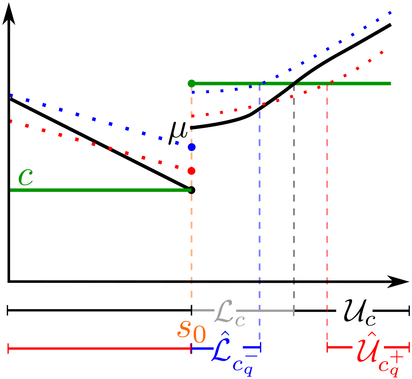
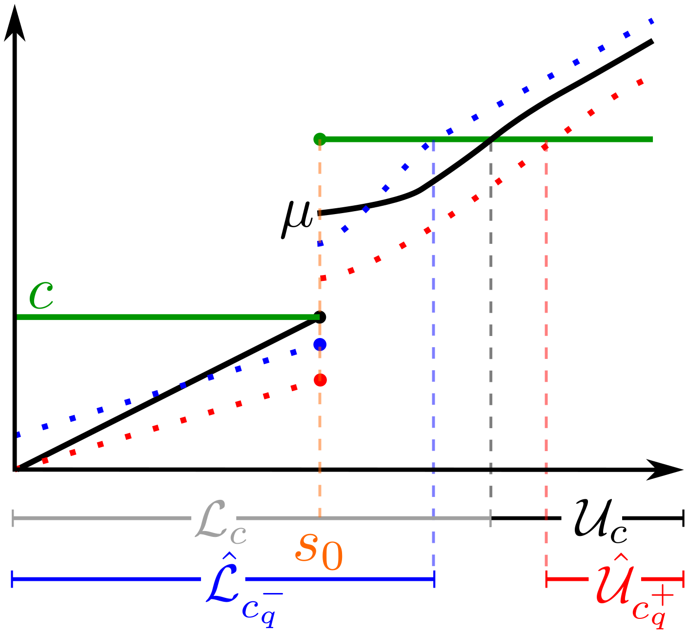
Figure 3: Illustration that Assumption (A4) cannot include points $s_{0}\in\mathfrak{u}^{-1}_{c}\setminus{\rm cl}\,\mu^{-1}_{c}$ although $G_{N}$ is continuous on a neighborhood of $\mathfrak{u}^{-1}_{c}\setminus{\rm cl}\,\mu^{-1}_{c}$. Although the bands defined by $\hat{\mu}_{N}\pm q\tau_{N}\sigma$ do not contain $\mu(s_{0})$ in both panels, all inclusions of the excursion sets are satisfied.

Setting $\mathcal{C}^{\pm}=\mathcal{F}(S)$ in Theorem 1 implies $S=\mathfrak{u}^{-1}_{\mathcal{C}}={\rm cl}\,\mu^{-1}_{\mathcal{C}}={\rm int}\,\mu^{-1}_{\mathcal{C}}$ and thus (A2)-(A4) are satisfied. This shows that the lower and upper excursion sets defined by thresholding the asymptotic $(1-\alpha)$-SCB obtained from an ULT yield $(1-\alpha)$-SCoPE sets over $\big{(}\mathcal{F}(S),\mathcal{F}(S)\big{)}$. Hence the next corollary is the asymptotic version of Proposition 1.

Corollary 1.

Let $\mathcal{C}^{\pm}=\mathcal{F}(S)$, $c^{\pm}_{q}=c\pm q\tau_{N}\sigma$ for $c\in\mathcal{F}(S)$ and assume (A1). Then

$$\lim_{N\rightarrow\infty}\mathbb{P}_{*}\left[\,\forall c\in\mathcal{F}(S):~{}\hat{\mathcal{L}}_{c_{q}^{-}}\subseteq\mathcal{L}_{c}~{}\wedge~{}\hat{\mathcal{\mathcal{U}}}_{c_{q}^{+}}\subseteq\mathcal{U}_{c}\,\right]=\mathbb{P}\Big{[}\,\max_{s\in S}|G(s)|\prec q\,\Big{]}\,.$$

The next corollary bounds the preimage of $\mu$ for several bands defined by functions $b_{k}^{\pm}\in\mathcal{F}(S)$ with $b_{k}^{-}(s)\leq b_{k}^{+}(s)$ for all $s\in S$ and $k\in\mathbb{N}$.

Corollary 2.

Let $b_{k}^{\pm}\in\mathcal{F}(S)$ for $k\in\mathbb{N}$ and $\mathcal{C}^{\pm}=\big{\{}\,b_{k}^{\pm}~{}|~{}k\in\mathbb{N}\,\big{\}}$. Define $b_{k,q}^{\pm}=b_{k}^{\pm}\pm q\tau_{N}\sigma$ for all $k\in\mathbb{N}$ and assume (A1). Then

$$\begin{split}\lim_{N\rightarrow\infty}\mathbb{P}_{*}\Big{[}\,\forall k\in\mathbb{N}:~{}\hat{\mathcal{L}}_{b_{k,q}^{-}}\subseteq\mathcal{L}_{b_{k}^{-}}~{}~{}\wedge~{}~{}\hat{\mathcal{U}}_{b_{k,q}^{+}}\subseteq\mathcal{U}_{b_{k}^{+}}\,\Big{]}=\mathbb{P}\Big{[}\,\mathfrak{T}_{\mathcal{C}^{-},\mathcal{C}^{+}}(G)\prec q\,\Big{]}\,.\end{split}$$

under (A2),(A3) / (A4).

Remark 10.

If $b^{\pm}=b^{\pm}_{k}$ for all $k\in\mathbb{N}$ with $b^{-}(s)\leq b^{+}(s)$ for all $s\in S$, then the above Corollary yields the following inclusion of partitions of $S$

$$\hat{\mathcal{L}}_{b_{q}^{-}}\subseteq\mathcal{L}_{b^{-}}\,,\quad\quad S\setminus\big{(}\hat{\mathcal{L}}_{b_{q}^{-}}\cup\hat{\mathcal{U}}_{b_{q}^{+}}\big{)}\subseteq S\setminus\big{(}\mathcal{L}_{b^{-}}\cup\mathcal{U}_{b^{+}}\big{)}\,,\quad\quad\hat{\mathcal{U}}_{b_{q}^{+}}\subseteq\mathcal{U}_{b^{+}}$$

which asymptotically is satisfied with at least the $q$ dependent inner probability on the r.h.s. of Corollary 2. If $b^{\pm}\in\mathbb{R}$ this becomes the more familiar:

$$\hat{\mathcal{L}}_{b_{q}^{-}}\subseteq\mu^{-1}\big{(}(\infty,b^{-})\big{)}\,,\quad\quad S\setminus\big{(}\hat{\mathcal{L}}_{b_{q}^{-}}\cup\hat{\mathcal{U}}_{b_{q}^{+}}\big{)}\subseteq\mu^{-1}\big{(}(b^{-},b^{+})\big{)}\,,\quad\quad\hat{\mathcal{U}}_{b_{q}^{+}}\subseteq\mu^{-1}\big{(}(b^{+},\infty)\big{)}\,.$$

Remark 11.

The special case $b^{\pm}=b^{\pm}_{k}$ for all $k\in\mathbb{N}$ and $b^{-}(s)\leq b^{+}(s)$ is particularly interesting. Readers familiar with [11, 9, 10] might spot the similarities between their limiting distributions and the limiting distribution of Corollary 2. This is not a coincidence as will be explained in Section 6 where we derive relevance and equivalence tests from Corollary 2.

Our last corollary generalizes the main theorem from [43]. Hence we assume that $S$ is compact and $\mu,c\in C(S)$ which yields that $\mathfrak{u}^{-1}_{\mp\{c\}}=\mu^{-1}_{c}$ and Assumption (A4) is always satisfied. Most importantly, we do not require their restrictive non-flatness Assumption 2.1(a).

Corollary 3.

Let $S$ be compact, $\mu,c\in C(S)$ and $c^{\pm}_{q}=c\pm q\tau_{N}\sigma$ for $q\in\mathbb{R}$. Assume that (A1)-(A2) hold for $\mathcal{C}=\{c\}$. Then

$$\lim_{N\rightarrow\infty}\mathbb{P}_{*}\left[\,\hat{\mathcal{L}}_{c_{q}^{-}}\subseteq\mathcal{L}_{c}~{}\wedge~{}\hat{\mathcal{\mathcal{U}}}_{c_{q}^{+}}\subseteq\mathcal{U}_{c}\,\right]=\mathbb{P}\big{[}\,\mathfrak{T}_{c}(G)\prec q\,\big{]}\,.$$

4.3 Estimating the Generalized Preimages and Bootstrapping the Quantile of SCoPE sets

Estimation of $q$ such that the families from Theorem 1 are $(1-\alpha)$-SCoPE sets requires estimation of $\mathfrak{u}^{-1}_{\pm\mathcal{C}}$ for $\mathcal{C}\subseteq\mathcal{F}(S)$.

Under (A1) we can then derive a Hausdorff-distance consistent estimator of $\mathfrak{u}^{-1}_{\pm\mathcal{C}}$ and $\mathfrak{u}^{-1}_{\mathcal{C}}$ by replacing $\mu$ by $\hat{\mu}_{N}$ in the definition of ${\rm cl}\,\mu^{-1}_{\mathcal{C}_{\eta}}$ and choosing $\eta$ depending on $N$ appropriately. More precisely, if $(k_{N})_{N\in\mathbb{N}}$ is a positive sequence converging to zero, we define the thickened-plugin-estimators of $\mathfrak{u}^{-1}_{\pm\mathcal{C}}$ and $\mathfrak{u}^{-1}_{\mathcal{C}}$ by

$$\begin{split}\hat{\mathfrak{u}}_{+\mathcal{C}}^{-1}&={\rm cl}\Big{\{}\,s\in S~{}\big{|}~{}\exists c\in\mathcal{C}:~{}0\leq\pm\big{(}\hat{\mu}_{N}(s)-c(s)\big{)}\leq k_{N}\tau_{N}\sigma(s)\,\Big{\}}\end{split}$$ (9)

and

$$\hat{\mathfrak{u}}_{\mathcal{C}}^{-1}=\hat{\mathfrak{u}}_{-\mathcal{C}}^{-1}\cup\hat{\mathfrak{u}}_{+\mathcal{C}}^{-1}={\rm cl}\big{\{}\,s\in S~{}\big{|}~{}\exists c\in\mathcal{C}:~{}|\,\hat{\mu}_{N}(s)-c(s)\,|\leq k_{N}\tau_{N}\sigma(s)\,\big{\}}\,.$$ (10)

If $\mu$ is continuous then The estimator $\hat{\mathfrak{u}}_{\mathcal{C}}^{-1}$ can be interpreted to be derived from a SCB which gives an interpretation of the factor $k_{N}$. Since $\mathbb{P}\big{[}\,\sup_{s\in S}|\tau_{N}^{-1}\big{(}\hat{\mu}_{N}(s)-\mu(s)|/\sigma(s)<k_{N}\,\big{]}=1-\tilde{\alpha}_{N}$ for some $\tilde{\alpha}_{N}\in(0,1)$ it is obvious from the definition of a $(1-\tilde{\alpha}_{N})$-SCB that

$$\mathbb{P}\Big{[}\,\mathfrak{u}_{\mathcal{C}}^{-1}\subseteq\hat{\mathfrak{u}}_{\mathcal{C}}^{-1}\,\Big{]}\geq 1-\tilde{\alpha}_{N}\,.$$

Identification of $k_{N}$ with the quantile of an SCB can help to justify the choice of $k_{N}$. Nevertheless, tuning $k_{N}$ by requiring $\mathbb{P}\big{[}\,\sup_{s\in S}|\tau_{N}^{-1}\big{(}\hat{\mu}_{N}(s)-\mu(s)|/\sigma(s)<k_{N}\,\big{]}=1-\tilde{\alpha}_{N}$ for a prespecified $1-\tilde{\alpha}_{N}>0.9$ can be (very) conservative (compare Appendix F).

The proof of consistency of the estimator (10) is similar to the proof of consistency of the estimator of the extremal set in [11]. It requires that $k_{N}$ converges to zero at an appropriate rate which implies that $\tilde{\alpha}_{N}$ goes to zero, too. We can interpret $\hat{\mathfrak{u}}_{\mathcal{C}}^{-1}\neq S$ as the rejection rule for a hypothesis test with null hypothesis $\mu\in\Gamma(\mathcal{C})$ and alternative hypothesis $\mu\notin\Gamma(\mathcal{C})$ at significance level at most $\tilde{\alpha}_{N}$. That $\tilde{\alpha}_{N}$ must converge to zero as $N$ tends to infinity is non-standard and might seem inappropriate at a first glance since usually the significance level in hypothesis testing is fixed to an acceptable threshold independent of $N$. This mathematical necessity resembles a philosophical question about practical data analysis: Is not the scientific cost for a Type I error in a large sample size experiment much higher than for a small data set because we tend to put more trust in large than small sample sizes? The core of the scientific method is reproducibility and evaluating coherence within our empirically collected knowledge. The later is usually less difficult to achieve for smaller sample sizes since in general such experiments are easier to repeat. Hence should large sample size experiments not pass higher standards if we want to draw conclusions from it?

Our next theorem strengthens this view from a mathematical perspective.

Theorem 2.

Let $S$ be compact and $(k_{N})_{N\in\mathbb{N}}$ be a positive sequence such that $\lim_{N\rightarrow\infty}k_{N}\tau_{N}=0$ and $\lim_{N\rightarrow\infty}k_{N}/\log\big{(}\tau_{N}^{-2}\big{)}=\kappa$ for some $\kappa>0$ and assume (A1). Then $d_{H}\big{(}\hat{\mathfrak{u}}_{\mathcal{C}}^{-1},\mathfrak{u}^{-1}_{\mathcal{C}}\big{)}\rightarrow 0$ in outer probability as $N$ tends to infinity and

$$\liminf_{N\rightarrow\infty}\mathbb{P}_{*}\Big{[}\mathfrak{u}^{-1}_{\pm\mathcal{C}}\subseteq\hat{\mathfrak{u}}_{\pm\mathcal{C}}^{-1}\Big{]}=1.$$ (11)

If additionally $\mu$ is continuous on ${\rm cl}\mu^{-1}_{\mathcal{C}_{\eta}}\setminus{\rm int}\mu^{-1}_{\mathcal{C}}$ for some $\eta>0$ and $\Gamma(\partial\mathcal{C})$ is closed, then $d_{H}\big{(}\hat{\mathfrak{u}}_{\pm\mathcal{C}}^{-1},\mathfrak{u}^{-1}_{\pm\mathcal{C}}\big{)}\rightarrow 0$ in outer probability as $N$ tends to infinity.

Remark 12.

The concept of the boundary $\partial\mathcal{C}$ of a set $\mathcal{C}\subseteq\mathcal{F}(S)$ is introduced in Appendix C. Note that this is not a topological boundary since we do not introduce a topology on $\mathcal{F}(S)$. The condition $\Gamma(\partial\mathcal{C})$ being closed is for example implied by $\Gamma(\mathcal{C})\subseteq S\times\mathbb{R}$ being closed or if there is a $\mathcal{C}^{\prime}\subseteq C(S)$ such that $\Gamma(\mathcal{C}^{\prime})=\Gamma(\mathcal{C})$.

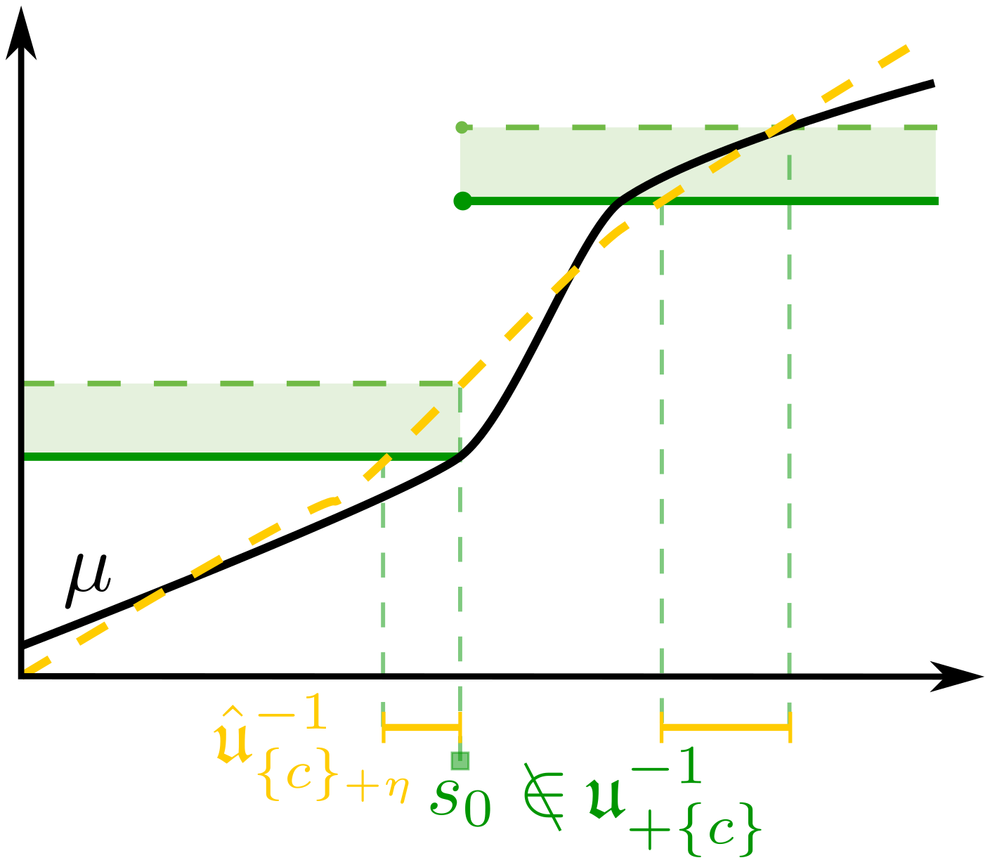
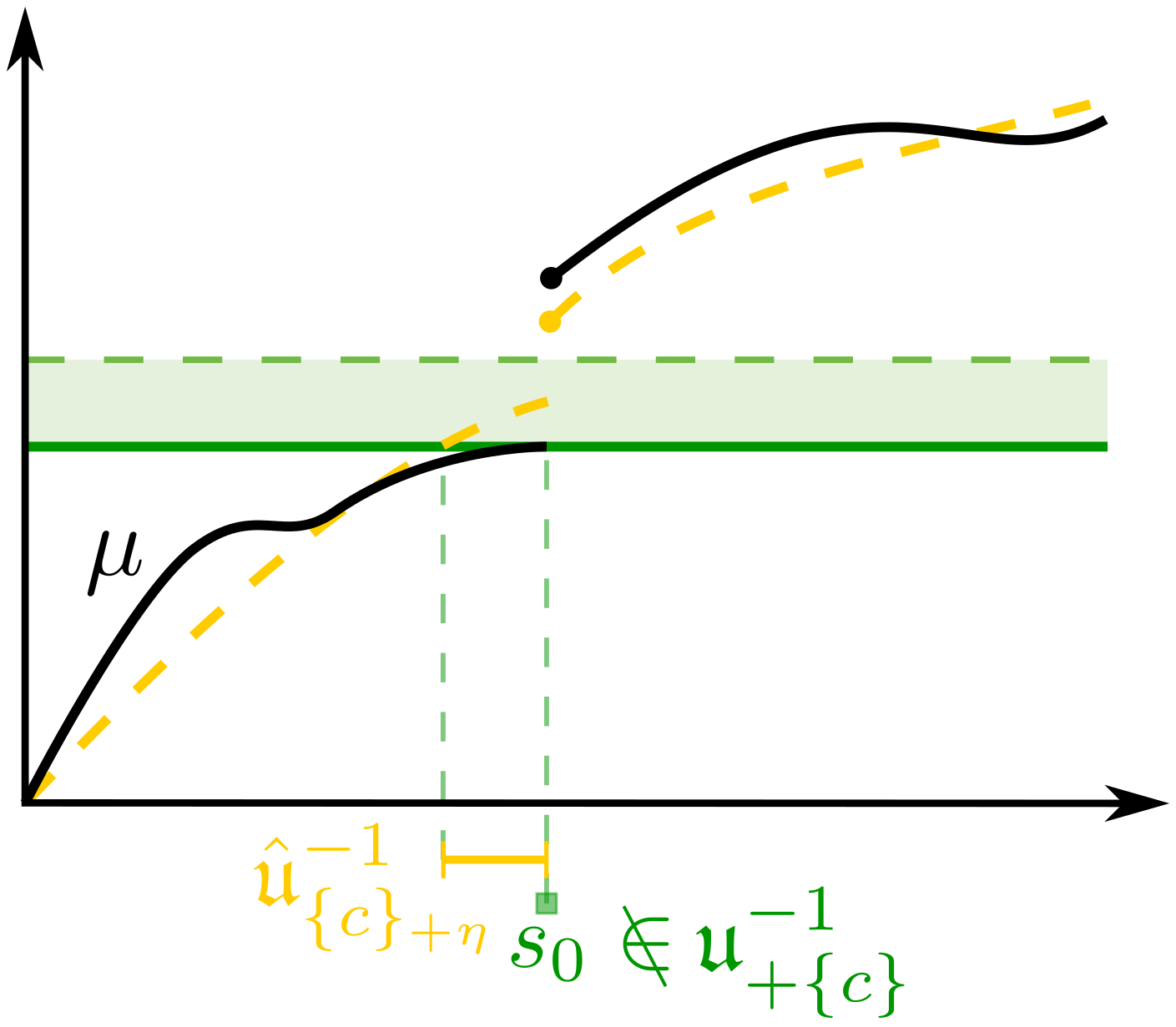
Figure 4: Illustration for $\mathcal{C}=\{c\}$ why the additional conditions to get Hausdorff convergence of $\hat{\mathfrak{u}}^{-1}_{\pm\mathcal{C}}$ to $\mathfrak{u}^{-1}_{\pm\mathcal{C}}$ are necessary. The problem is that $s_{0}\notin\mathfrak{u}^{-1}_{+\mathcal{C}}$ and $\mu$ is getting arbitrary close to $c$ in any neighbourhood of $s_{0}$ with the wrong sign.

In principle, the Hausdorff consistency results of the above theorem allow us to estimate the quantile of SCoPE sets using the bootstrap along the lines described in [11]. A general strategy (not necessarily the best in a given probabilistic model) to achieve this is to show within the assumed probabilistic model that realizations of a bootstrap processes $B_{N}^{(1)},\ldots,B^{(R)}_{N}$ can be obtained which satisfy

$$\begin{split}\Big{(}G_{N},B_{N}^{(1)},\ldots,B_{N}^{(R)}\Big{)}\rightsquigarrow\Big{(}G,G^{(1)},\ldots,G^{(R)}\Big{)}\end{split}$$ (12)

weakly in $\big{(}\ell^{\infty}({\rm cl}\,\mu^{-1}_{\mathcal{C}_{\tilde{\eta}}})\big{)}^{R+1}$. Here $G^{(1)},\ldots,G^{(R)}$ are i.i.d. copies of $G$. A helpful simplifying idea to achieve this for complicated statistics can be functional delta residuals [46]. Combining (12) with Theorem 2 and a generalization of Lemma B.3 from [11] (compare also Appendix A.3) yields for two sequences of sets $\big{(}\mathcal{C}_{N}\big{)}_{N\in\mathbb{N}}$ and $\big{(}\mathcal{D}_{N}\big{)}_{N\in\mathbb{N}}$ in $S$ converging in outer probability in Hausdorff-distance to $\mathcal{C},\mathcal{D}\subseteq S$ that (with slight abuse of the notation (5))

$$\begin{split}\Big{(}T_{\mathcal{C}_{N},\mathcal{D}_{N}}(G_{N}),T_{\mathcal{C}_{N},\mathcal{D}_{N}}\big{(}B_{N}^{(1)}\big{)},\ldots,&T_{\mathcal{C}_{N},\mathcal{D}_{N}}\big{(}B_{N}^{(R)}\big{)}\Big{)}\\ &\rightsquigarrow\Big{(}\mathfrak{T}_{\mathcal{C},\mathcal{D}}(G),\mathfrak{T}_{\mathcal{C},\mathcal{D}}\big{(}G^{(1)}\big{)},\ldots,\mathfrak{T}_{\mathcal{C},\mathcal{D}}\big{(}G^{(R)}\big{)}\Big{)}\end{split}$$

weakly in $\mathbb{R}^{R+1}$. Here $\mathfrak{T}_{\mathcal{C},\mathcal{D}}\big{(}G^{(1)}\big{)},\ldots,\mathfrak{T}_{\mathcal{C},\mathcal{D}}\big{(}G^{(R)}\big{)}$ are i.i.d. copies of $\mathfrak{T}_{\mathcal{C},\mathcal{D}}(G)$.

5 Applications of SCoPE Sets

Theorem 1 is affluent in interpretations because it allows to extract information about any combination of excursion sets of $\mu$ and thereby allows to draw conclusion about its image. Hence we give only a short glance into possible applications.

5.1 Confidence Regions for Contour lines

SCoPE sets offer the possibility to provide confidence regions for contour lines of a target function $\mu$ derived from an estimator $\hat{\mu}_{N}$. Assume that $c_{1},\ldots,c_{K}\in\mathbb{R}$ are the contour values of interest, then applying Theorem 5 to the sets $\mathcal{C}^{\pm}=\{s\mapsto c_{k}~{}|~{}k=1,\ldots,K\}$ provides the simultaneous ${(1-\alpha)}$-confidence regions $\hat{C}^{1-\alpha}_{k}=S\setminus\left(\hat{\mathcal{L}}_{c_{k}^{-q_{\alpha}}}\cup\hat{\mathcal{U}}_{c_{k}^{+q_{\alpha}}}\right)$ for the sets $C_{k}=\{s\in S~{}|~{}\mu(s)=c_{k}\}$, if $q_{\alpha}$ is chosen such that

$$\mathbb{P}\Bigg{[}\,\max_{s\in\mathfrak{u}^{-1}_{\mathcal{C}}}|G(s)|<q_{\alpha}\,\Bigg{]}={1-\alpha}\,.$$

Corollary 4.

Let $\mathcal{C}=\{s\mapsto c_{k}~{}|~{}k=1,\ldots,K\}$, $\mathfrak{u}^{-1}_{\mathcal{C}}\neq\emptyset$ and assume (A1) and that the random variable $\max_{s\in\mathfrak{u}^{-1}_{\mathcal{C}}}|G(s)|$ has a continuous cdf. Then

$$\lim_{N\rightarrow\infty}\mathbb{P}_{*}\Big{[}\,\forall k\in\{1,\ldots,K\}:~{}C_{k}\subseteq\hat{C}^{1-\alpha}_{k}\,\Big{]}={1-\alpha}\,.$$

under (A2),(A3) / (A4).

Remark 13.

Controlling the inclusion of excursion sets implies control of the inclusion of contour lines. However, the reverse is not true, as already observed in [43].

5.2 Regions of Interest Analysis

In applications, such as neuroimaging, the researcher might be interested in reporting only the results of a statistical analysis specific to regions of interest (RoI). Usually, however, it is not evident before collecting the data, which RoI from a predefined set needs to be reported. SCoPE sets offer a solution to this problem.

A set of RoIs consists of subsets $R_{k}\subset S$, $k\in\{1,\ldots,K\}$. Define for each $k\in\{1,\ldots,K\}$ the indicators of a RoI by

$$\chi_{k}^{\pm}(s)=\begin{cases}1,&\text{ for }s\in R_{k}\\ \mp\infty,&\text{ else }\end{cases}\,.$$

Any $b_{k}\in\mathcal{F}(S)$ can be adapted to a RoI $R_{k}$ by defining $c_{k}^{\pm}(s)=\chi_{k}^{\pm}(s)b_{k}(s)$ which implies

$$\mathcal{L}_{c_{k}^{-}}\subseteq R_{k}\,,\quad\mathcal{U}_{c_{k}^{+}}\subseteq R_{k}\,,\quad\hat{\mathcal{L}}_{c_{k,q}^{-}}\subseteq R_{k}\,,\quad\hat{\mathcal{U}}_{c_{k,q}^{+}}\subseteq R_{k}$$

for $c_{k,q}^{\pm}=c_{k}^{\pm}+q\tau_{N}\sigma$. Applying Theorem 1 to $\mathcal{C}^{\pm}=\big{\{}\,c_{k}^{\pm}~{}|~{}k\in\{1,\ldots,K\}\,\big{\}}$ allows the researcher to inspect the confidence subsets of the RoI specific lower and upper excursion sets and report only the results of the interesting RoI’s without making mistakes due to multiple comparisons. Similarly, more complicated questions can be answered about the level sets on the RoI’s by including more RoI adapted functions into $\mathcal{C}^{\pm}$.

5.3 Scheffé Type Inference For Multiple Linear Regression

Interestingly, Theorem 1 offers novel simultaneous inference strategies for contrasts in multiple linear regression models. Here we only discuss SCoPE sets over $\big{(}\{0\},\{0\}\big{)}$. More complicated SCoPE sets can be found in Appendix E.2. Moreover, we restrict ourselves to the case of homoscedastic Gaussian errors, although our results extend to more complicated settings.

Let $(X_{N})_{N\in\mathbb{N}}\in\mathbb{R}^{N\times K}$ be a sequence of design matrices of rank $K<N$, $(\tau_{N})_{N\in\mathbb{N}}$ be a sequence satisfying $\lim_{N\rightarrow\infty}\tau_{N}^{-2}(X_{N}^{T}X_{N})^{-1}=\mathfrak{X}\in\mathbb{R}^{K\times K}$ with $\mathfrak{X}$ invertible and the observations $\bm{y}_{N}$ are generated from a linear model, i.e., $\bm{y}_{N}\sim\mathcal{N}\left(X_{N}\bm{\beta},\xi^{2}I_{N\times N}\right)$ with $\xi\in\mathbb{R}_{>0}$. Recall that $\hat{\bm{\beta}}_{N}=(X_{N}^{T}X_{N})^{-1}X^{T}_{N}\bm{y}_{N}$, $N\in\mathbb{N}$, is the uniformly minimum-variance unbiased estimator (UMVU) of $\bm{\beta}$. Usually not $\bm{\beta}$, but linear contrasts $\mu(\bm{a})=\bm{a}^{T}\bm{\beta}$, $\bm{a}\in\mathbb{R}^{K}$, are of interest. Interpreting $\bm{a}\in\mathbb{R}^{K}$ as the parameter set, we define a stochastic process indexed in $\mathbb{R}^{K}$ and its asymptotic variance by $\hat{\mu}_{N}(\bm{a})=\bm{a}^{T}\hat{\bm{\beta}}_{N}$, $\sigma^{2}(\bm{a})=\xi^{2}\bm{a}^{T}\mathfrak{X}\bm{a}$. Since all involved quantities are Gaussian and continuous in $\bm{a}$, we obtain

$$G_{N}(\bm{a})=\frac{\hat{\mu}_{N}(\bm{a})-\mu(\bm{a})}{\tau_{N}\xi\sqrt{\bm{a}^{T}\mathfrak{X}\bm{a}}}\rightsquigarrow G(\bm{a})$$ (13)

weakly in $C\big{(}\mathbb{R}^{K}\big{)}$, where $G$ is the zero-mean Gaussian process with covariance function

$$\mathfrak{c}(\bm{a},\bm{b})=\frac{\bm{a}^{T}\mathfrak{X}\bm{b}}{\sqrt{\bm{a}^{T}\mathfrak{X}\bm{a}}\sqrt{\bm{b}^{T}\mathfrak{X}\bm{b}}}\,,~{}~{}~{}\text{ for }\bm{a},\bm{b}\in\mathbb{R}^{K}\,.$$

Since $G_{N}(\bm{a})=G_{N}(\tilde{\bm{a}})$ and $G(\bm{a})=G(\tilde{\bm{a}})$ with $\tilde{\bm{a}}=\bm{a}/\|\bm{a}\|$, the domain of the processes should actually be the compact space $\mathbb{S}^{K-1}=\{\bm{a}\in\mathbb{R}^{K}~{}|~{}\|\bm{a}\|=1\}$ instead of $\mathbb{R}^{K}$.

A standard task in multiple linear regression is finding contrasts $\bm{b}\in\mathbb{S}^{K-1}$ using the observations $\bm{y}_{N}$ such that with high probability $\bm{b}\in\{\bm{a}\in\mathbb{S}^{K-1}~{}|~{}\bm{a}^{T}\bm{\beta}\neq 0\}$. This can be achieved for example using SCBs [40]. The asymptotic analogue of Scheffé’s ${(1-\alpha)}$-SCBs for contrasts are given by the intervals with endpoints

$$\hat{\mu}(\bm{a})\pm q_{1-\alpha,K}\sigma(\bm{a})=\bm{a}^{T}\hat{\bm{\beta}}_{N}\pm\tau_{N}q_{1-\alpha,K}\xi\sqrt{\bm{a}^{T}\mathfrak{X}\bm{a}}\,,$$ (14)

where $q_{1-\alpha,K}^{2}$ is the $(1-\alpha)$-quantile of a $\chi^{2}_{K}$-distributed random variable [35, eq. (8.71)]. Based on this and using Theorem 8.5 from [35] the asymptotic version of Scheffé’s test rejects the null hypothesis of $\bm{a}^{T}\bm{\beta}=0$ for all $\bm{a}\in\mathbb{S}^{K-1}$ at significance level $\alpha$, if

$$\xi^{-2}\big{(}\hat{\bm{\beta}}_{N}^{T}\mathfrak{X}^{T}\mathfrak{X}\hat{\bm{\beta}}_{N}\big{)}^{2}>\tau_{N}^{2}q_{1-\alpha,K}^{2}\,,$$

which is equivalent to the existence of $\bm{a}\in\mathbb{S}^{K-1}$ such that zero is not contained in the interval given by (14). Corollary 1 shows that this SCB contains more information than allowing us to perform a valid hypothesis test for $\bm{a}^{T}\bm{\beta}=0$ for all $\bm{a}\in\mathbb{S}^{K-1}$. We actually know that

$$\mathbb{P}\left[\forall c\in\mathcal{F}\big{(}\mathbb{R}^{K}\big{)}:~{}\hat{\mathcal{L}}_{c-q_{1-\alpha,K}K\sigma}\subseteq\mathcal{L}_{c}~{}\wedge~{}\hat{\mathcal{U}}_{c+q_{1-\alpha,K}K\sigma}\subseteq\mathcal{U}_{c}\,\right]=1-\alpha\,.$$

This implies for $c\equiv 0$ that all contrasts $\bm{b}\in\mathbb{S}^{K-1}$ contained in either of the two sets

$$\begin{split}\hat{\mathcal{L}}_{-\tau_{N}q_{1-\alpha,K}\sigma}&=\Big{\{}\,\bm{a}\in\mathbb{S}^{K-1}:~{}\bm{a}^{T}\hat{\bm{\beta}}<-\tau_{N}q_{1-\alpha,K}\xi\sqrt{\bm{a}^{T}\mathfrak{X}\bm{a}}\,\Big{\}}\,,\\ \hat{\mathcal{U}}_{\tau_{N}q_{1-\alpha,K}\sigma}&=\Big{\{}\,\bm{a}\in\mathbb{S}^{K-1}:~{}\bm{a}^{T}\hat{\bm{\beta}}>\tau_{N}q_{1-\alpha,K}\xi\sqrt{\bm{a}^{T}\mathfrak{X}\bm{a}}\,\Big{\}}\end{split}$$

are asymptotically with probability at least $1-\alpha$ correctly discovered to be non-zero contrasts, i.e., $\bm{b}\in\{\bm{a}\in\mathbb{S}^{K-1}~{}|~{}\bm{a}^{T}\bm{\beta}\neq 0\}=\mathcal{L}_{c}\cup\mathcal{U}_{c}$. This result holds independent of the actual value of $\bm{\beta}$. The drawback is low detection power since it constructs confidence subsets for more functions than just $c\equiv 0$. The power can be improved by applying Corollary 3.

Corollary 5.

Assume the multiple linear regression model depending on $N$ as defined above. Let $c(\bm{a})=0$ for all $\bm{a}\in\mathbb{S}^{K-1}$ and $q\in\mathbb{R}_{\geq 0}$. Then

$$\lim_{N\rightarrow\infty}\mathbb{P}\left[\,\hat{\mathcal{L}}_{-\tau_{N}q\sigma}\subseteq\mathcal{L}_{0}~{}\wedge~{}\hat{\mathcal{U}}_{\tau_{N}q\sigma}\subseteq\mathcal{U}_{0}\,\right]=\chi^{2}\big{(}q^{2},K-1+\mathds{1}_{\bm{\beta}=0}\big{)}\,.$$

Here $\mathds{1}_{\bm{\beta}=0}$ is the indicator function, i.e., one, if $\bm{\beta}=0$, and zero else, and $u\mapsto\chi^{2}(u,k)$ is the cumulative distribution function of a $\chi^{2}_{k}$-distributed random variable.

Corollary 5 suggests a more powerful strategy to detect non-zero contrasts which is tailored to control the excursion sets for $c\equiv 0$. Let $q_{1-\alpha,K-1}^{2}$ be the $(1-\alpha)$-quantile of a $\chi^{2}_{K-1}$-distributed random variable. Then Corollary 5 yields

$$\lim_{N\rightarrow\infty}\mathbb{P}\left[\,\hat{\mathcal{L}}_{-\tau_{N}q_{1-\alpha,K-1}\sigma}\subseteq\mathcal{L}_{0}~{}\wedge~{}\hat{\mathcal{U}}_{\tau_{N}q_{1-\alpha,K-1}\sigma}\subseteq\mathcal{U}_{0}\,\right]=\begin{cases}1-\alpha\,,&\text{ if }\bm{\beta}\neq 0\\ \chi^{2}\big{(}q_{1-\alpha,K-1}^{2},K\big{)}\,,&\text{ if }\bm{\beta}=0\end{cases}\,.$$

This means that, if $\bm{\beta}\neq 0$, all discovered contrasts are with probability ${1-\alpha}$ correctly identified to be non-zero. On the other hand, if $\bm{\beta}=0$, it holds that $\mathcal{L}_{0}=\mathcal{U}_{0}=\emptyset$. Thus, asymptotically the probability to find any non-zero contrast, i.e., $\hat{\mathcal{L}}_{-\tau_{N}q_{1-\alpha,K-1}\sigma}\cup\hat{\mathcal{U}}_{\tau_{N}q_{1-\alpha,K-1}\sigma}\neq\emptyset$, is $1-\chi^{2}\big{(}q_{1-\alpha,K-1}^{2},K\big{)}$. The latter tests the statistical hypothesis $\bm{a}^{T}\bm{\beta}=0$ for all $\bm{a}\in\mathbb{S}^{K-1}$ with asymptotic significance level $1-\chi^{2}\big{(}q_{1-\alpha,K-1}^{2},K\big{)}$. Since $q_{1-\alpha,K-1}^{2}<q_{1-\alpha,K}^{2}$, it is more likely to discover non-zero contrasts within the SCoPE sets framework than using Scheffé’s SCBs. The price to pay is that for $\bm{\beta}=0$ incorrectly discovering at least one non-zero contrast is slightly larger than $\alpha$, yet this probability can be quantified.

As an illustration assume ${1-\alpha}=0.95$, $k=4$ and the researcher uses $(1-\alpha)$-SCoPE sets over $(\{0\},\{0\})$ to find non-zero contrasts. This means that, if the true $\bm{\beta}\neq 0$, then all discovered contrasts are with probability $0.95$ correctly identified to be non-zero contrasts, and that the null hypothesis of $\bm{\beta}=0$ can be rejected at significance level $1-\chi^{2}\big{(}q_{0.95,3}^{2},4\big{)}\approx 0.1$. The latter means that, if the researcher is unlucky and the true $\bm{\beta}$ is equal to zero, then having discovered any non-zero contrasts is an event which happens with probability $\approx 0.1$.

5.4 A Simple Example of a SCoPE sets Analysis

The last paragraph of the previous section highlighted a different view through SCoPE sets on statistical hypothesis testing. The key observation was that the estimated $q_{1-\alpha,K}$ to obtain $(1-\alpha)$-SCoPE sets for $\big{(}\{0\},\{0\}\big{)}$ can be used to judge the plausibility of the statistical hypothesis $\bm{\beta}=0$, since the asymptotic probability of discovering any non-zero contrast is given by $1-\chi^{2}\big{(}q_{1-\alpha,K-1}^{2},K\big{)}$. We will call such a value an insignificance value because it helps judging the plausibility of our discoveries under the probabilistic model and allows to declare discoveries ”insignificant”. The idea of this section is to showcase on a simple probabilistic model what we call a insignificance analysis which from our viewpoint should be reported together with SCoPE sets.

Let us assume our observations are $\bm{y}_{1},\ldots,\bm{y}_{N}$ and a reasonable probabilistic model is given by $\bm{y}_{1},\ldots,\bm{y}_{N}\sim\mathcal{N}\big{(}\bm{\mu},{\rm diag}(\bm{\sigma}^{2})\big{)}$ iid. with $\bm{y}_{n}=(y_{n1},\ldots,y_{nJ})$, $n\in\{1,\ldots,N\}$, for unknown $\bm{\mu}=(\mu_{1},\ldots,\mu_{J})\in\mathbb{R}^{J}$ and $\bm{\sigma}=(\sigma_{1},\ldots,\sigma_{J})\in\mathbb{R}^{J}$. A question of interest might be which $\mu_{j}$, $j\in\{1,\ldots,J\}$, are non-zero. In this model for given $k_{N}$ the plugin-thickening estimator of $\bm{\mu}^{-1}_{0}=\big{\{}j\in\{1,\ldots,J\}~{}|~{}\bm{\mu}_{j}=0\big{\}}$ from Section 4.3 is

$$\hat{\bm{\mu}}^{-1}_{0}=\Big{\{}j\in\{1,\ldots,J\}~{}\big{|}~{}|\hat{\bm{\mu}}_{j}|\leq\tfrac{k_{N}}{\sqrt{N}}\Big{\}}\,.$$

There are two natural choices of the parameter $k_{N}$ obtained from the discussion in Section 4.3. First, $k_{N}=\log(N)/\kappa$ for some $\kappa>0$ and second, $k_{N}$ being an estimate of the quantile for a $(1-\beta)$-SCB, i.e., satisfying

$$\mathbb{P}\Bigg{[}\max_{j\in\{1,\ldots,J\}}|X_{j}|\leq k_{N}\Bigg{]}=1-\beta$$

for $X_{1},\ldots,X_{J}$ independent $t_{N-1}$-distributed. The critical quantile from Corollary 3 for $(1-\alpha)$-SCoPE sets over $\big{(}\{0\},\{0\}\big{)}$ is given by

$$q_{1-\alpha}=\inf\Big{\{}q~{}\big{|}~{}\Phi(q)^{\#\bm{\mu}^{-1}_{0}}>1-\alpha\Big{\}}$$

with $\Phi(q)=\mathbb{P}\big{[}\mathcal{N}(0,1)\leq q\big{]}$ and $\#A$ denotes the cardinality of the set $A$. An estimator of this quantile for unknown $\bm{\sigma}$ in the considered probabilistic model is

$$\hat{q}^{k_{N}}_{1-\alpha}=\inf\Big{\{}q~{}\big{|}~{}\Phi_{N-1}(q)^{\#\hat{\bm{\mu}}^{-1}_{0}}>1-\alpha\Big{\}}$$

with $\Phi_{N-1}(q)=\mathbb{P}\big{[}X\leq q\big{]}$ where $X\sim t_{N-1}$ is Student’s $t$-distributed with $N-1$ degrees of freedom. Another estimator tailored to this model can be given using an idea from [45]. Here the author proposed to estimate the number $m_{0}$ of true null hypotheses using the distribution of the $p$-values $p_{1},\ldots,p_{N}$ from the tests on the hypothesis $H_{0}:\mu_{j}=0$ by

$$\hat{m}_{0}=2\#\big{\{}j\in\{1,\ldots,J\}~{}|~{}p_{j}\geq 0.5\big{\}}\,.$$ (15)

In our model the $p$-values are derived from Student’s $t_{N-1}$-distribution. The resulting estimator of the quantile is then

$$\hat{q}^{St}_{1-\alpha}=\inf\Big{\{}q~{}\big{|}~{}\Phi_{N-1}(q)^{\hat{m}_{0}}>1-\alpha\Big{\}}\,.$$

Simulation results of the validity of SCoPE sets for different $\bm{\mu}$ and the estimator $\hat{q}^{St}_{1-\alpha}$ of $q$ and the estimators of $q$ based on different $k_{N}$ are provided in Appendix F. They demonstrate that SCoPE sets using a reasonable estimator of the quantile $q$ are a more powerful FWER controlling method to detect non-zero $\mu_{j}$’s than Hommel’s procedure for i.i.d. samples [22].

In Fig. 5 we report the discoveries obtained from SCoPE sets for samples of size $N=100$. In the top row we used the estimator (10) with $k_{N}=\log(N)/10$ and detected one location to be non-zero. In the bottom row we computed SCoPE sets for the another data set, but we used $k_{N}=\log(N)/10$ (bottom left) which detects $30$ non-zero locations and $k_{N}=\log(N)/3$ (bottom right) which detects $24$ non-zero locations.

We propose to accept these discoveries only after inspection of insignificance values. A first useful set of insignificance values obtained for the estimator $\hat{q}_{1-\alpha}$ of $q_{1-\alpha}$ for the discussed probabilistic model is

$$\begin{split}IV_{M,m}^{\hat{q}}&=\mathbb{P}\Big{[}\,\#\big{\{}\,j^{\prime}\in\{1,\ldots,M\}~{}\big{|}~{}|X_{j}|\geq\hat{q}_{1-\alpha}\,\big{\}}\geq m\,\Big{]}\end{split}$$ (16)

for $X_{1},\ldots,X_{J}\sim t_{N-1}$ i.i.d. and $m\in\{1,\ldots,M\}$. We will write $IV_{M}^{\hat{q}}=IV_{M,1}^{\hat{q}}$. These insignificance values are as $p$-values counterfactual conditionals, i.e., they answer a question of the form: What would be true under certain (hypothetical) circumstances. More precisely, the values $IV_{M,m}^{\hat{q}}$ tell the researcher the probability of having at least $m$ discoveries given the probabilistic model would be true, the threshold would be fixed to $\hat{q}_{1-\alpha}$ and $\bm{\mu}=0$. Similarly, $IV_{M}^{\hat{q}}$ is the probability of having at least one false discovery if it would be the case that $\#\mu^{-1}_{0}=M$ and in repeated experiments the researcher would use the same fixed threshold $\hat{q}$. Additionally it might be helpful to report the observational insignificance values

$$\begin{split}IV_{M,m}^{obs}&=\mathbb{P}\Bigg{[}\,\#\Big{\{}\,j^{\prime}\in\{1,\ldots,M\}~{}\big{|}~{}|X_{j}|\geq\min_{j\in\hat{\mathcal{L}}_{-\hat{q}\hat{\sigma}/\sqrt{N}}~{}\cup~{}\hat{\mathcal{U}}_{\hat{q}\hat{\sigma}/\sqrt{N}}}\sqrt{N}|\hat{\mu}_{j}/\hat{\sigma}_{j}|\,\Big{\}}\geq m\,\Bigg{]}\end{split}$$ (17)

for $M\in\{1,\ldots,J\}$ and $m\in\{1,\ldots,M\}$. The quantity $IV_{M}^{obs}$ is the probability of having at least one false discovery with height of the smallest observed discovery if the probabilistic model would be true and $\#\mu^{-1}_{0}$ would be $M$.

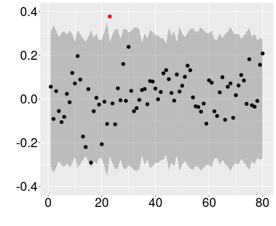
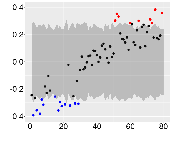
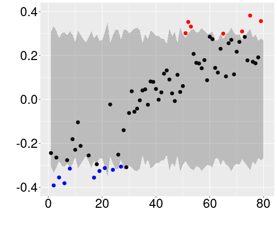
Figure 5: Examples of discoveries obtained from $90\%$-SCoPE sets over $(0,0)$ for the model described in this section with sample size $N=100$. The choice of $k_{N}$ for the estimator (10) is given in Table 1. The points represent the sample mean $\hat{\mu}_{j}=N^{-1}\sum y_{jn}$. The red points are contained in $\hat{\mathcal{U}}_{\hat{q}\sqrt{N}\hat{\sigma}}$ and the blue points in $\hat{\mathcal{L}}_{-\hat{q}\sqrt{N}\hat{\sigma}}$. Thus, the corresponding $j$’s represent the locations at which the SCoPE sets discovered a non-zero population mean. Points inside the grey area cannot be decided upon whether the population mean is smaller or larger than $0$.

For the SCoPE sets reported in Fig. 5 some insignificance values are summarized in Table 1. Judging from these the researcher should declare the discovery in the top left figure to be insignificant because there is a probability of $IV_{80}^{\hat{q}}=24.5\%$ to have at least one discovery if it would be the case that $\bm{\mu}=0$ and a discovery of at least the observed height at the discovery would still appear with a probability of $IV_{80}^{obs}=14.1\%$. The top right figure has the same $IV_{80}^{\hat{q}}$. Thus, the researcher should be suspicious about his discovery. However, the observational insignificance value $IV_{80}^{obs}=0.3\%$ states that it is very unlikely that this discovery appeared by chance alone in the worst case counterfactual scenario where $\bm{\mu}=0$. Hence this discovery should not be declared insignificant by the researcher although the choice of $k_{N}$ is questionable. Unfortunately in this particular case he commits an error of the first kind, but repeating the same or similar experiments as good scientific practice requires would correct the erroneous decision.

For the bottom left figure $IV_{80}^{\hat{q}}$ and even $IV_{80}^{obs}$ are large. Since $IV_{80,4}^{\hat{q}}\approx 0$, the researcher can conclude that the observed amount of discoveries most probably did not appeared by chance and that there should be at least around $26$ discoveries. Problematic is that $IV_{80-\hat{m}_{1}}^{\hat{q}}=39.4$ means that it is highly likely to make a false discovery on the set $\mu^{-1}_{0}$ if the true number of discoveries would be $\hat{m}_{1}=30$. Even if the true number of possible discoveries would be $80-\hat{m}_{0}=48$ then the probability of making a false discovery is still $IV_{\hat{m}_{0}}^{\hat{q}}=27.1\%$. Here it is implausible to claim that the inclusion statement is actually controlled at probability $90\%$ for $k_{N}=\log(100)/10$. Only if $\#\mu^{-1}_{0}\leq 10$ the control of the inclusion statement would be $IV_{10}^{\hat{q}}\approx 10\%$. For the bottom right figure this is different. Here $IV_{80-\hat{m}_{1}}^{\hat{q}}=19.8\%$ and $IV_{\hat{m}_{0}}^{\hat{q}}=IV_{32}^{\hat{q}}=11.5\%$ and hence $k_{N}=\log(N)/3$ seems to be plausible since the data suggests $\#\mu^{-1}_{0}$ to be around $\hat{m}_{0}=32$. This insignificance analysis is compatible with our simulation results. Choosing $k_{N}=\log(N)/3$ is a decent choice since the simulated probability of satisfying the inclusion statement of the SCoPE sets is $\approx 88\%$ while this probability is only $\approx 77\%$ for $k_{N}=\log(N)/10$ (Appendix F Table 3).

A similar analysis can be designed if SCoPE sets over $(\{c^{-}\},\{c^{+}\})$ are conducted for $c^{-}<c^{+}$, however, in that case obtaining worst case values of $\bm{\mu}$ is not as simple as in the above scenario because these values can take values within the interval $[c^{-},c^{+}]$. Still we can guard ourselves against counterfactual conditional scenarios which seem to be plausible.

Panel	$\mathbf{k}_{N}$	$\mathbf{\hat{q}}$	$IV_{80}^{obs}$	$IV_{80}^{\hat{q}}$	$IV_{80-\hat{m}_{1}}^{\hat{q}}$	$IV_{\hat{m}_{0}}^{\hat{q}}$	SCoPE	Hommel	BH
top left	$\log(100)/10$	3.00	14.1	24.5	-	-	0 / 1	0 / 0	0 / 0
top right	$\log(100)/10$	3.00	0.3	24.5	-	-	0 / 1	0 / 0	0 / 0
bottom left	$\log(100)/10$	2.64	50.1	53.1	39.4	27.1	30 / 0	21 / 0	42 / 0
bottom right	$\log(100)/3$	2.97	23.1	26.1	19.8	11.5	24 / 0	21 / 0	42 / 0

´

Table 1: Information on the estimated quantile, the used $k_{N}$ in estimator (10) and four helpful insignificance values for the $90\%$-SCoPE sets over $(0,0)$ reported in Fig. 5. The last three rows contain how many true discoveries and false discoveries different statistical inference tools output. Here BH denotes the Benjamini-Hochberg procedure which controls the FDR.

6 Hypothesis Testing using SCoPE Sets

This section gives details on how to use SCoPE sets as a test statistic for relevance and equivalence tests. In general, we do not recommend our tests since the questions about the preimage of $\mu$ which are conveyed in a statistical hypothesis can be directly answered by appropriate SCoPE sets which offer a more intuitive interpretation. We include the test interpretation only to compare SCoPE sets to the existing literature. Hereafter, we assume that the functions $b^{+},b^{-}\in\mathcal{F}(S)$ satisfy $b^{-}(s)\leq b^{+}(s)$ for all $s\in S$ and for simplicity in notation we assume whenever $\mathcal{C}\in\mathcal{F}(S)$ is specified that $\mathfrak{u}_{\mathcal{C}}=\mathfrak{u}_{\pm\mathcal{C}}$ which follows for example from the continuity assumption on $\mu$ given in Theorem 2. Moreover, if $\mathbf{H}_{0,s}$ and $\mathbf{H}_{1,s}$ are null and alternative hypotheses for $s\in S$ and we have a statistical test which decides between these two alternatives from data, then we define the set of true null hypotheses $\mathcal{H}_{0}$ and true alternative hypotheses $\mathcal{H}_{1}$ and their estimates as

$$\begin{split}\mathcal{H}_{0}&=\big{\{}s\in S:~{}\mathbf{H}_{0,s}\text{ is true }\big{\}}\,,~{}~{}~{}\hat{\mathcal{H}}_{0}=\big{\{}s\in S:~{}\mathbf{H}_{0,s}\text{ is not rejected }\big{\}}\\ \mathcal{H}_{1}&=\big{\{}s\in S:~{}\mathbf{H}_{1,s}\text{ is true }\big{\}}\,,~{}~{}~{}\hat{\mathcal{H}}_{1}=\big{\{}s\in S:~{}\mathbf{H}_{0,s}\text{ is rejected }\big{\}}\,.\end{split}$$

6.1 Relevance Tests

We first want to construct a global relevance Test (grT) based on SCoPE sets, i.e., a test on the alternatives

$$\begin{split}\mathbf{H}^{rel}_{0}\mathbf{:}~{}~{}\forall s\in S:~{}\mu(s)\in\big{[}b^{-}(s),b^{+}(s)\big{]}~{}~{}~{}\text{ vs.}~{}~{}~{}\mathbf{H}^{rel}_{1}\mathbf{:}~{}~{}\exists s\in S:~{}\mu(s)\notin\big{[}b^{-}(s),b^{+}(s)\big{]}\,.\end{split}$$

Because $\mathbf{H}^{rel}_{0}$ being true implies $\mathcal{L}_{b^{-}}=\emptyset=\mathcal{U}_{b^{+}}$ an intuitive test using SCoPE sets is to decide in favor of $\mathbf{H}^{rel}_{0}$ if $\hat{\mathcal{L}}_{b_{q}^{-}}=\emptyset=\hat{\mathcal{U}}_{b_{q}^{+}}$ and reject it if $\hat{\mathcal{L}}_{b_{q}^{-}}\neq\emptyset$ or $\hat{\mathcal{U}}_{b_{q}^{+}}\neq\emptyset$. Here $b_{q}^{\pm}=b^{\pm}\pm\tau_{N}q\sigma$ for $q>0$. At a first glance Theorem 1 with $\mathcal{C}^{\pm}=\{b^{\pm}\}$ and assuming $\hat{\mu}_{N}$ satisfies a $\mathcal{F}(S)$-ULT suggests that we can determine a critical quantile $q_{\alpha}$ such that the above test asymptotically has significance level $\alpha$ since it implies for all $q$ that

$$\begin{split}\limsup_{N\rightarrow\infty}\mathbb{P}^{*}\left[\,\hat{\mathcal{L}}_{b_{q}^{-}}\neq\emptyset~{}\vee~{}\hat{\mathcal{U}}_{b_{q}^{+}}\neq\emptyset\,\right]&=1-\liminf_{N\rightarrow\infty}\mathbb{P}_{*}\left[\,\hat{\mathcal{L}}_{b_{q}^{-}}=\emptyset~{}\wedge~{}\hat{\mathcal{U}}_{b_{q}^{+}}=\emptyset\,\right]\\ &=1-\liminf_{N\rightarrow\infty}\mathbb{P}_{*}\left[\,\hat{\mathcal{L}}_{b_{q}^{-}}\subseteq\mathcal{L}_{b^{-}}~{}\wedge~{}\hat{\mathcal{U}}_{b_{q}^{+}}\subseteq\mathcal{U}_{b^{+}}\,\right]\\ &\leq 1-\mathbb{P}\Big{[}\,\mathfrak{T}_{b^{-},b^{+}}(G)<q\,\Big{]}\,.\end{split}$$

Unfortunately, the r.h.s. is zero for all $q$ in the highly likely scenario that $\mathfrak{u}^{-1}_{b^{-}}\cup\mathfrak{u}^{-1}_{b^{+}}=\emptyset$. Thus, usually it is impossible to tune $q$ as desired. In order to remove this ambiguity we got inspired by [11]. Note that for $b^{\pm}_{\Delta^{e}}=b^{\pm}\pm\max(\,\Delta_{-}^{e},\Delta_{+}^{e}\,)$ with $\Delta_{\pm}^{e}=\sup_{s\in S}\pm\mu(s)\mp b^{\pm}(s)$ we have by definition that $\mathcal{L}_{b^{-}}=\mathcal{L}_{b^{-}_{\Delta^{e}}}=\emptyset$ and $\mathcal{U}_{b^{+}}=\mathcal{U}_{b^{+}_{\Delta^{e}}}=\emptyset$ if $\mathbf{H}^{rel}_{0}$ is true. Thus, the idea is to choose $q_{\alpha}^{gr}$ to be the smallest $q$ such that $\mathbb{P}\big{[}\,\mathfrak{T}_{b_{\Delta^{e}}^{-},b_{\Delta^{e}}^{+}}(G)\geq q\,\big{]}\leq\alpha$. The latter is unique because either $\mathfrak{u}^{-1}_{b_{\Delta^{e}}^{-}}$ or $\mathfrak{u}^{-1}_{b_{\Delta^{e}}^{+}}$ is not the empty set. This follows directly from the definition of $b_{\Delta^{e}}^{\pm}$ and the definition of the generalized preimage because there is a sequence $(s_{k})_{k\in\mathbb{N}}$ such that $|b_{\Delta^{e}}^{-}(s_{k})-\mu(s_{k})|\rightarrow 0$ or $|b_{\Delta^{e}}^{+}(s_{k})-\mu(s_{k})|\rightarrow 0$. The following theorem is a generalization of the test strategies proposed in [11, 10, 13] and is providing an asymptotical procedure for a global relevance test over $S$. Its proof is similar to the proof of Theorem 4 which generalizes the upcoming theorem to provide a local relevance test controlling the FWER in the strong sense and therefore we leave the proof of the following result to the reader.

Theorem 3.

Let $\mathcal{C}^{\pm}=\big{\{}b_{\Delta^{e}}^{\pm}\big{\}}$ and assume (A1). Recall that $\mathbf{H}^{rel}_{0}$ is true if $\Delta^{e}\leq 0$ and false otherwise. For $\alpha\in(0,1)$, the grT discussed above with the quantile $q_{\alpha}^{gr}$ satisfies

• Let $\Delta^{e}=0$. Assume (A2) and (A3), then

  $$\begin{split}\limsup_{N\rightarrow\infty}&\,\,\mathbb{P}^{*}\big{[}\,\mathbf{H}^{rel}_{0}\text{ is rejected }\,\big{]}\leq\alpha\,.\end{split}$$

  Assume (A4), then

  $$\begin{split}\liminf_{N\rightarrow\infty}&\,\,\mathbb{P}_{*}\big{[}\,\mathbf{H}^{rel}_{0}\text{ is rejected }\,\big{]}\geq\mathbb{P}\Big{[}\,\mathfrak{T}_{b_{\Delta}^{-},b_{\Delta}^{+}}(G)>q_{\alpha}^{gr}\,\Big{]}\,.\end{split}$$

  Let $\Delta^{e}<0$, then $\lim_{N\rightarrow\infty}\,\,\mathbb{P}^{*}\big{[}\,\mathbf{H}^{rel}_{0}\text{ is rejected }\,\big{]}=0$.

• Let $\Delta^{e}>0$, then $\lim_{N\rightarrow\infty}\,\,\mathbb{P}_{*}\big{[}\,\mathbf{H}^{rel}_{0}\text{ is rejected }\,\big{]}=1$ .

In order to see that this result generalizes the testing strategy from [11] ([13, 10] can be treated similarly) we translate their notations into the notations of this article. Assume that $\hat{\mu}_{N}$ is an estimator of a continuous function $\mu$ satisfying a ULT in $C(S)$ with $\sigma\equiv 1$ and $S=[0,1]$. This estimator could be the difference of the sample means from [11]. Based on their Theorem 3.1 they propose to test the global null hypothesis $\mathbf{H}_{0}^{rel}$ for $b^{\pm}\equiv\pm b$, $b\geq 0$, by rejecting the null hypothesis if $\|\hat{\mu}_{N}\|_{\infty}>b+\frac{q_{\alpha}^{gr}}{\sqrt{N}}$. That $q_{\alpha}^{gr}$ is identical to their quantile $u_{1-\alpha,\mathcal{E}}$ [11, eq. (3.14)] can be seen from the fact that their extremal sets $\mathcal{E}^{-}$ and $\mathcal{E}^{+}$ satisfy

$$\mathcal{E}^{\pm}=\big{\{}s\in S~{}|~{}\mu(s)=\pm\|\mu\|_{\infty}\big{\}}=\mu^{-1}_{\pm\|\mu\|_{\infty}}=\mathfrak{u}^{-1}_{b^{\pm}_{\Delta^{e}}}.$$

As it can be easily verified that $\hat{\mathcal{L}}_{b_{q_{\alpha}^{gr}}^{-}}\neq\emptyset$ or $\hat{\mathcal{U}}_{b_{q_{\alpha}^{gr}}^{+}}\neq\emptyset$ is equivalent to $\|\hat{\mu}_{N}\|_{\infty}>b+\frac{q_{\alpha}^{gr}}{\sqrt{N}}$, Theorem 3 indeed generalizes their testing strategy to allow adaptation to some scaling function $\sigma$, allows $b^{\pm}$ and $\mu$ to be possibly discontinuous functions and clarifies what kind of continuity is required in the ULT.

Using Theorem 1 we can similarly construct a strong $\alpha$-FWER local relevance Test (lrT), i.e., a multiple hypothesis test for the alternatives

$$\begin{split}\mathbf{H}^{rel}_{0,s}\mathbf{:}~{}~{}\mu(s)\in\big{[}b^{-}(s),b^{+}(s)\big{]}~{}~{}~{}\text{ vs. }~{}~{}~{}\mathbf{H}^{rel}_{1,s}\mathbf{:}~{}~{}\mu(s)\notin\big{[}b^{-}(s),b^{+}(s)\big{]}\,,\end{split}$$

which controls the FWER in the strong sense. The main difference is that we replace $\Delta^{e}$ by the smallest $\Delta>0$ such that $\mathfrak{u}^{-1}_{b^{-}+\Delta}\cup\mathfrak{u}^{-1}_{b^{+}-\Delta}\neq\emptyset$ and still $\mathcal{L}_{b^{-}}=\mathcal{L}_{b^{-}+\Delta}$ and $\mathcal{U}_{b^{+}}=\mathcal{U}_{b^{+}-\Delta}$.

Definition 9.

Let $\Delta_{\pm}=\inf_{s\in S}\big{|}\mu(s)-b^{\pm}(s)\big{|}$, $\Delta=\min\{\Delta_{-},\Delta_{+}\}$ and $b_{\Delta}^{\pm}=b^{\pm}\mp\Delta$. For $\alpha\in(0,1)$, let $q_{\alpha}^{lr}$ be such that $\mathbb{P}\big{[}\,\mathfrak{T}_{b_{\Delta}^{-},b_{\Delta}^{+}}(G)\geq q_{\alpha}^{lr}\,\big{]}\leq\alpha$ provided that $\mathfrak{u}^{-1}_{b_{\Delta}^{-}}\cup\mathfrak{u}^{-1}_{b_{\Delta}^{+}}\neq\emptyset$ and otherwise set $q_{\alpha}^{lr}=0$. Define $b_{\alpha,r}^{\pm}=b^{\pm}\pm\tau_{N}q_{\alpha}^{lr}\sigma$. The lrT based on SCoPE sets accepts $\mathbf{H}^{rel}_{0,s}$ for all $s\in S\setminus\big{(}\hat{\mathcal{L}}_{b_{\alpha,r}^{-}}\cup\hat{\mathcal{U}}_{b_{\alpha,r}^{+}}\big{)}$ and rejects it for all $s\in\hat{\mathcal{L}}_{b_{\alpha,r}^{-}}~{}\cup~{}\hat{\mathcal{U}}_{b_{\alpha,r}^{+}}$.

Remark 14.

For the lrT it can happen that even if $\mathcal{H}_{0}\neq\emptyset$ that $\mathfrak{u}^{-1}_{b_{\Delta}^{-}}\cup\mathfrak{u}^{-1}_{b_{\Delta}^{+}}=\emptyset$ (Fig. 6).

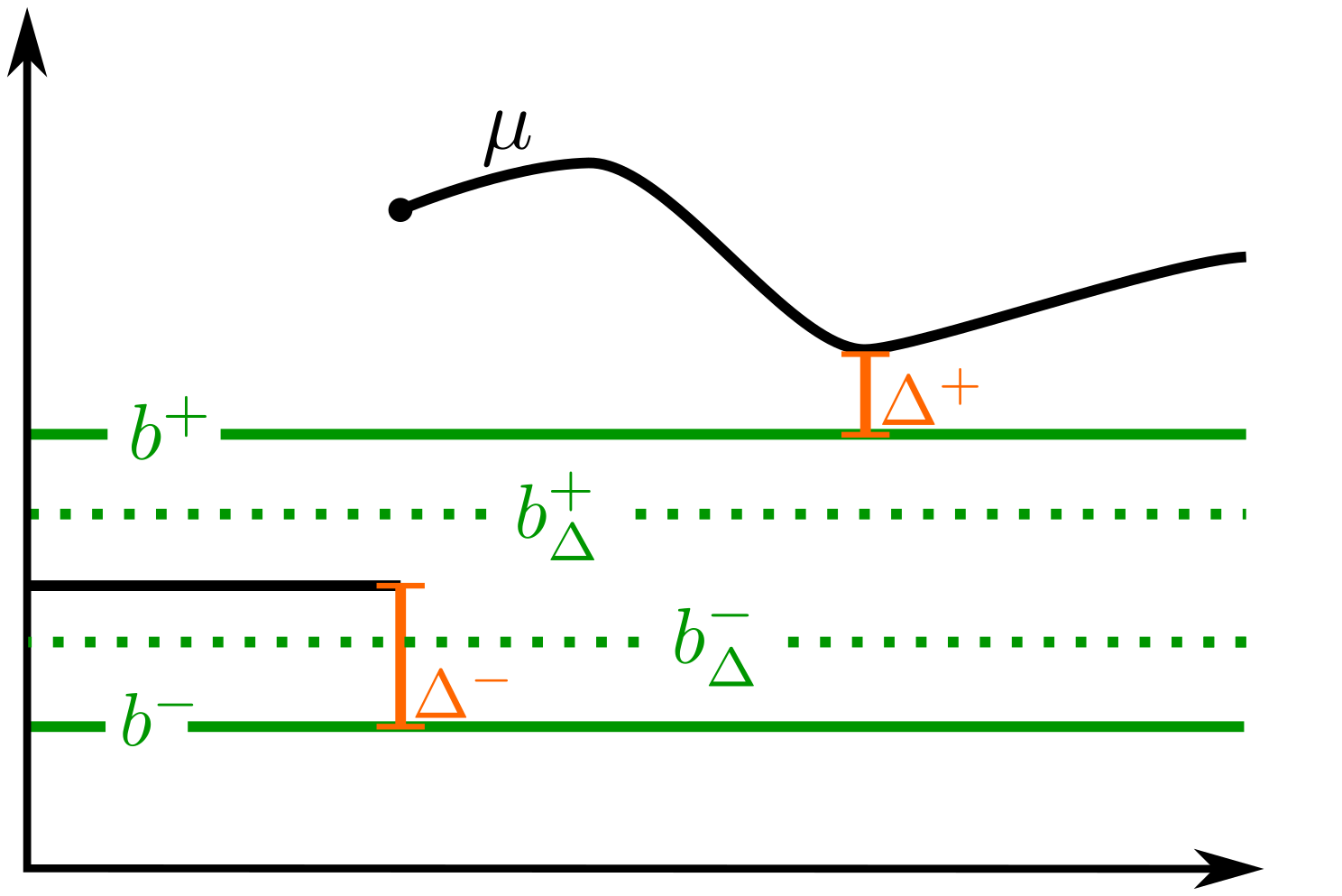
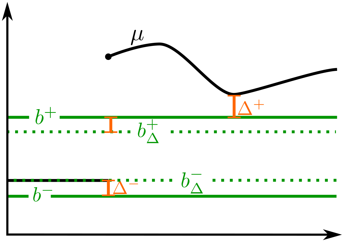
Figure 6: Illustration that the critical set $\mathfrak{u}^{-1}_{b_{\Delta}^{-}}\cup\mathfrak{u}^{-1}_{b_{\Delta}^{+}}$ can be either empty or non-empty. Left: The critical set is empty because $\mathbf{H}_{1,s}^{rel}$ is true at the point $s$ with minimal distance between $\mu$ and $b^{-}$ and $b^{+}$. Right: The critical set is non-empty because $\mathbf{H}_{0,s}^{rel}$ is true at the point $s$ with minimal distance between $\mu$ and $b^{-}$ and $b^{+}$.

Theorem 4.

Consider the lrT from Definition 9, set $\mathcal{C}^{\pm}=\big{\{}b_{\Delta}^{\pm}\big{\}}$ and assume (A1).

• Assume $\mathcal{H}_{0}\neq\emptyset$, (A2) and (A3), then

  $$\begin{split}\limsup_{N\rightarrow\infty}&\,\,\mathbb{P}^{*}\big{[}\,\exists s\in\mathcal{H}_{0}:~{}s\in\hat{\mathcal{H}}_{1}\,\big{]}\leq\alpha\,.\end{split}$$

  Assume (A4), then

  $$\begin{split}\liminf_{N\rightarrow\infty}&\,\,\mathbb{P}_{*}\big{[}\,\forall s\in\hat{\mathcal{H}_{1}}:~{}s\in\mathcal{H}_{1}\,\big{]}\geq 1-\alpha\,.\end{split}$$

• Assume $\Delta=0$, (A4) and either $\mathcal{H}_{0}=S$ or $\inf_{s\in S}\big{(}\,b^{+}(s)-b^{-}(s)\,\big{)}\geq M>0$. Then

  $$\begin{split}\liminf_{N\rightarrow\infty}\mathbb{P}_{*}\big{[}\,\exists s\in\mathcal{H}_{0}:~{}s\in\hat{\mathcal{H}}_{1}\,\big{]}\geq\mathbb{P}\Big{[}\,\mathfrak{T}_{b_{\Delta}^{-},b_{\Delta}^{+}}(G)>q_{\alpha}^{lr}\,\Big{]}\,.\end{split}$$

• Assume $\Delta=0$, $\eta_{N}\rightarrow 0$ and $\tau_{N}^{-1}\eta_{N}\rightarrow\infty$ as $N\rightarrow\infty$. If $\mathcal{H}_{1}^{\eta_{N}}=\mathcal{L}_{b^{-}-\eta_{N}}\cup\mathcal{U}_{b^{+}+\eta_{N}}$, then

  $$\begin{split}&\liminf_{N\rightarrow\infty}\mathbb{P}_{*}\big{[}\,\forall s\in\mathcal{H}_{1}^{\eta_{N}}:~{}s\in\hat{\mathcal{H}}_{1}\,\big{]}=1\,.\end{split}$$

• Assume $\Delta>0$, then

  $$\begin{split}\lim_{N\rightarrow\infty}\mathbb{P}^{*}\big{[}\,\exists s\in\mathcal{H}_{0}:~{}s\in\hat{\mathcal{H}}_{1}\,\big{]}=0\,,~{}~{}~{}~{}\lim_{N\rightarrow\infty}\mathbb{P}_{*}\big{[}\,\forall s\in\mathcal{H}_{1}:~{}s\in\hat{\mathcal{H}}_{1}\,\big{]}=1\,.\end{split}$$

Remark 15.

One sided hypothesis tests can be obtained by setting either $b^{-}\equiv-\infty$ or $b^{+}\equiv\infty$. The two-sided point hypotheses for a single $b\in\mathcal{F}(S)$ is the special case of the lrT with $b^{\pm}=b$. By Theorem 4 it is asymptotically a consistent strong $\alpha$-FWER test which rejects the null hypothesis at $s\in S$ if and only if $\left|\frac{\hat{\mu}_{N}(s)-b(s)}{\tau_{N}\sigma(s)}\right|>q_{\alpha}^{lr}$ with $q_{\alpha}^{lr}$ such that $\mathbb{P}\Big{[}\,\mathfrak{T}_{b_{\Delta}^{-},b_{\Delta}^{+}}(G)\geq q_{\alpha}^{lr}\,\Big{]}\leq\alpha$. Hence this test is more powerful than the standard asymptotic single-step test which replaces $\mathfrak{T}_{b_{\Delta}^{-},b_{\Delta}^{+}}(G)$ by $\max_{s\in S}|G(s)|$ in the computation of the quantile.

The main difference between the grT and the lrT based on SCoPE sets is the definition of the critical quantile under $\mathbf{H}_{1}^{rel}$ because in this scenario $\mathfrak{u}^{-1}_{\pm\|\mu\|_{\infty}}\neq\mathfrak{u}^{-1}_{b_{\Delta}^{\pm}}$ (Fig. 7). Interestingly, it is impossible to claim that either of the two tests has a higher statistical power. The reason is that the quantiles depend on the covariance structure of $G$ on $\mathfrak{u}^{-1}_{-\|\mu\|_{\infty}}\cup\mathfrak{u}^{-1}_{+\|\mu\|_{\infty}}$ and $\mathfrak{u}^{-1}_{b_{\Delta}^{-}}\cup\mathfrak{u}^{-1}_{b_{\Delta}^{+}}$ respectively. The set $\mathfrak{u}^{-1}_{-\|\mu\|_{\infty}}\cup\mathfrak{u}^{-1}_{+\|\mu\|_{\infty}}$ is for many $\mu\in\ell^{\infty}(S)$ a singleton $\{s^{*}\}$ where $s^{*}$ is the unique global extreme point of $\mu$. In this case the asymptotic theoretical quantile is simply the quantile of $G(s^{*})$. If the variance of $G$ is assumed constant over $S$ this means that the grT is often more powerful than the lrT to detect a departure from $\mathbf{H}_{0}^{rel}$. However, it is possible to construct alternatives such that the roles are reversed (Fig. 7).

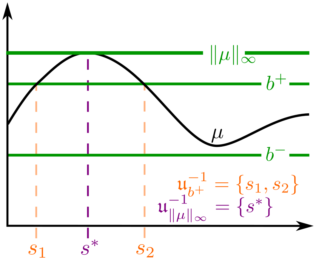
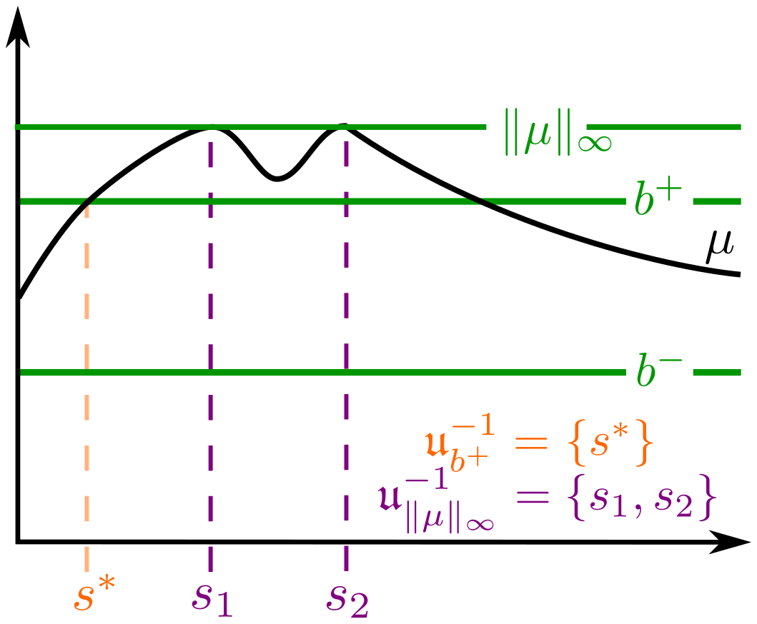
Figure 7: Illustration of the critical sets $\mathfrak{u}^{-1}_{b^{+}}$ and $\mathfrak{u}^{-1}_{\|\mu\|_{\infty}}$ under $\mathbf{H}_{1}^{rel}$.

6.2 Equivalence Tests

We assume in this section additionally that $\inf_{s\in S}|\,b^{+}(s)-b^{-}(s)\,|>0$. An equivalence Test (eT) is a test on the hypothesis

$$\begin{split}\mathbf{H}^{eqv}_{0}\mathbf{:}~{}~{}\exists s\in S:~{}\mu(s)\notin\big{[}b^{-}(s),b^{+}(s)\big{]}~{}~{}~{}\text{ vs. }~{}~{}~{}\mathbf{H}^{eqv}_{1}\mathbf{:}~{}~{}\forall s\in S:~{}\mu(s)\in\big{[}b^{-}(s),b^{+}(s)\big{]}\,.\end{split}$$

The eT based on SCoPE sets is similar to the gRT based on SCoPE sets. The main change is that the rejection condition becomes the acceptance condition and that the sign in the definition of $b^{\pm}_{\Delta}$ is changed such that at least one of the shifted curves touches the most extreme values $\pm\|\mu\|_{\infty}$ of $\mu$ under $\mathbf{H}^{eqv}_{0}$, compare Fig. 8.

Definition 10.

Let $\alpha\in(0,1)$ and $b_{\Delta}^{\pm}=b^{\pm}\pm\Delta^{e}$, where $\Delta^{e}$ has been defined in Theorem 3. Let $q_{\alpha}^{e}$ be such that $\mathbb{P}\big{[}\,\mathfrak{T}_{b_{\Delta}^{-},b_{\Delta}^{+}}(G)\leq q_{\alpha}^{e}\,\big{]}\leq\alpha\,.$ Define $b_{\alpha,e}^{\pm}=b^{\pm}\pm\tau_{N}q_{\alpha}^{e}\sigma$. The eT based on SCoPE sets accepts $\mathbf{H}^{eqv}_{0}$ if $\hat{\mathcal{L}}_{b_{\alpha,e}^{-}}~{}\cup~{}\hat{\mathcal{U}}_{b_{\alpha,e}^{+}}\neq\emptyset$ and rejects it otherwise.

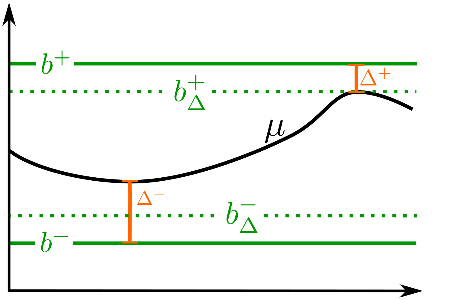
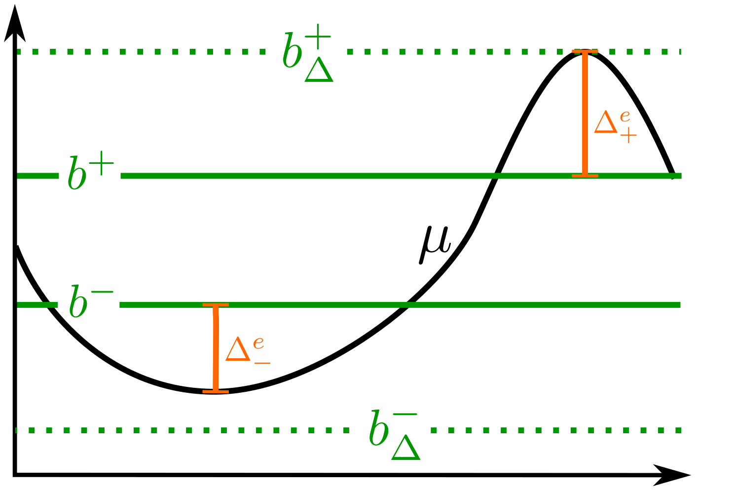
Figure 8: Left: Illustration of the difference in the definition of $b^{\pm}_{\Delta}$ for the grT and the eT. Right: grT if $\mathbf{H}_{0}^{rel}$ is true. Left: eT if $\mathbf{H}_{0}^{eqv}$ is true.

Theorem 5.

Consider the eT from Definition 10. Let $\mathcal{C}^{\pm}=\big{\{}b_{\Delta^{e}}^{\pm}\big{\}}$ and assume (A1). Recall that $\mathbf{H}^{eqv}_{0}$ is true if $\Delta^{e}\geq 0$ and false otherwise.

• Let $\Delta^{e}=0$. Assume (A4), then

  $$\begin{split}\limsup_{N\rightarrow\infty}&\,\,\mathbb{P}^{*}\big{[}\,\mathbf{H}^{eqv}_{0}\text{ is rejected }\,\big{]}\leq\alpha\,.\end{split}$$

  Assume (A2) and (A3), then

  $$\begin{split}\liminf_{N\rightarrow\infty}&\,\,\mathbb{P}_{*}\big{[}\,\mathbf{H}^{eqv}_{0}\text{ is rejected }\,\big{]}\geq\mathbb{P}\big{[}\,\mathfrak{T}_{b_{\Delta}^{-},b_{\Delta}^{+}}(G)<q_{\alpha}^{e}\,\big{]}\,.\end{split}$$

  Let $\Delta^{e}>0$, then $\lim_{N\rightarrow\infty}\,\,\mathbb{P}^{*}\big{[}\,\mathbf{H}^{eqv}_{0}\text{ is rejected }\,\big{]}=0\,.$

• Let $\Delta^{e}<0$, then $\lim_{N\rightarrow\infty}\,\,\mathbb{P}_{*}\big{[}\,\mathbf{H}^{eqv}_{0}\text{ is rejected }\,\big{]}=1\,.$

Remark 16.

If we assume that $\mu,\hat{\mu}_{N},b^{\pm}\in C([0,1])$ and $\sigma\equiv 1$, then simple algebra shows that the testing strategy proposed in Definition 10 is identical to the testing strategy from [9], because $\hat{\mathcal{L}}_{b_{\alpha,e}^{-}}=\emptyset$ and $\hat{\mathcal{U}}_{b_{\alpha,e}^{+}}=\emptyset$ is equivalent to

$$\max\left(\,\sup_{s\in S}\hat{\mu}_{N}(s)-b^{+}(s),~{}\sup_{s\in S}b^{-}(s)-\hat{\mu}_{N}(s)\,\right)\leq\tau_{N}q_{\alpha}^{e}$$

and their theoretical quantile is identical to $q_{\alpha}^{e}$. The only difference is that in the definition of the quantile they use $"<"$, which is irrelevant since in their probabilistic model the cumulative distribution function of $\mathfrak{T}_{b_{\Delta}^{+},b_{\Delta}^{-}}(G)$ being continuous. Thus, our eT based on SCoPE sets generalizes the testing strategy proposed in [9].

6.3 Local Equivalence Tests

If the alternatives of an lrT are interchanged, i.e.,

$$\begin{split}\mathbf{H}^{leqv}_{0,s}\mathbf{:}~{}~{}\mu(s)\notin\big{[}b^{-}(s),b^{+}(s)\big{]}~{}~{}~{}\text{vs.}~{}~{}~{}\mathbf{H}^{leqv}_{1,s}\mathbf{:}~{}~{}\mu(s)\in\big{[}b^{-}(s),b^{+}(s)\big{]}\,,\end{split}$$

we call a test on this alternatives a local equivalence Test (leT). Interestingly, an eT is not a global leT because a global leT tries to answer the question whether $\mu$ is always outside of the band defined by $b^{-}$ and $b^{+}$.

Definition 11.

Let $b_{\Delta}^{\pm}=b^{\pm}\pm\Delta$ with the $\Delta$ from Definition 9. For $\alpha\in(0,1)$, let $q_{\alpha}^{le}$ be such that $\mathbb{P}\big{[}\,\mathfrak{T}_{b_{\Delta}^{+},b_{\Delta}^{-}}(G)\geq q_{\alpha}^{le}\,\big{]}=\alpha\,$ provided that $\mathfrak{u}^{-1}_{b_{\Delta}^{-}}\cup\mathfrak{u}^{-1}_{b_{\Delta}^{+}}\neq\emptyset$, otherwise $q_{\alpha}^{le}=0$. Define $b_{\alpha,le}^{\pm}=b^{\pm}\mp\tau_{N}q_{\alpha}^{le}\sigma$. The leT based on SCoPE sets accepts $\mathbf{H}_{0,s}^{leqv}$ for all $s\in\hat{\mathcal{L}}_{b_{\alpha,le}^{+}}\cup\hat{\mathcal{U}}_{b_{\alpha,le}^{-}}$ and rejects it for all $s\in S\setminus\big{(}\hat{\mathcal{L}}_{b_{\alpha,le}^{+}}\cup\hat{\mathcal{U}}_{b_{\alpha,le}^{-}}\big{)}$.

Remark 17.

The changes between the lrT and the leT based on SCoPE sets are subtle. First, the condition for acceptance and rejection are exchanged as well as the role of $b^{-}_{\alpha,le}$ and $b^{+}_{\alpha,le}$ in the lower and upper excursions and $b_{\Delta}^{-}$ and $b_{\Delta}^{+}$ in the limit distribution. Second, there is a sign change in $b_{\alpha,le}^{\pm}$ compared to $b^{\pm}_{\alpha,r}$.

Theorem 6.

Consider the test from Definition 11. Let $\mathcal{C}^{\pm}=\big{\{}\,b_{\Delta}^{\pm}\,\big{\}}$, assume (A1) and $\inf_{s\in S}\big{(}\,b^{+}(s)-b^{-}(s)\,\big{)}>0$.

• Assume $\mathcal{H}_{0}\neq\emptyset$, (A2) and (A3), then

  $$\begin{split}\limsup_{N\rightarrow\infty}&\,\,\mathbb{P}^{*}\big{[}\,\exists s\in\mathcal{H}_{0}:~{}s\in\hat{\mathcal{H}}_{1}\,\big{]}\leq\alpha\,.\end{split}$$

  Assume (A4), then

  $$\begin{split}\liminf_{N\rightarrow\infty}&\,\,\mathbb{P}_{*}\big{[}\,\forall s\in\hat{\mathcal{H}_{1}}:~{}s\in\mathcal{H}_{1}\,\big{]}\geq 1-\alpha\,.\end{split}$$

• Assume $\Delta=0$ and (A4), then

  $$\begin{split}\liminf_{N\rightarrow\infty}\mathbb{P}_{*}\big{[}\,\exists s\in\mathcal{H}_{0}:~{}s\in\hat{\mathcal{H}}_{1}\,\big{]}\geq\mathbb{P}\big{[}\,\mathfrak{T}_{b_{\Delta}^{+},b_{\Delta}^{-}}(G)>q_{\alpha}^{le}\,\big{]}\end{split}$$

• Assume $\Delta=0$, $\eta_{N}\rightarrow 0$, $\tau_{N}^{-1}\eta_{N}\rightarrow\infty$ as $N\rightarrow\infty$ and $\mathcal{H}_{1}^{\eta_{N}}=\mathcal{L}_{b^{+}-\eta_{N}}\cap~{}\mathcal{U}_{b^{-}+\eta_{N}}$, then

  $$\begin{split}&\liminf_{N\rightarrow\infty}\mathbb{P}_{*}\big{[}\,\forall s\in\mathcal{H}_{1}^{\eta_{N}}:~{}s\in\hat{\mathcal{H}}_{1}\,\big{]}=1\,.\end{split}$$

• Assume $\Delta>0$, then

  $$\begin{split}\limsup_{N\rightarrow\infty}\mathbb{P}^{*}\big{[}\,\exists s\in\mathcal{H}_{0}:~{}s\in\hat{\mathcal{H}}_{1}\,\big{]}=0\,,~{}~{}~{}~{}\liminf_{N\rightarrow\infty}\mathbb{P}_{*}\big{[}\,\forall s\in\mathcal{H}_{1}:~{}s\in\hat{\mathcal{H}}_{1}\,\big{]}=1\end{split}$$

Remark 18.

A standard approach for an eT of a parameter $\mu\in\mathbb{R}$ is the Principle of Confidence Interval Inclusion (PCII) [53, Chapter 3.1]. Let $X$ denote the observations and $C_{\pm}(X;\alpha)$ the one-sided $(1-\alpha)$-confidence bounds for $\mu$, i.e.,

$$\mathbb{P}\big{[}\,\mu\in\big{(}\!-\infty,\,C_{-}(X;\alpha)\,\big{)}\,\big{]}=\mathbb{P}\big{[}\,\mu\in\big{(}\,C_{+}(X;\alpha),\infty\,\big{)}\,\big{]}=\alpha\,.$$

Let $b^{-}<b^{+}$. The alternatives $\mathbf{H}_{0}:\mu\notin(b^{-},b^{+})$ vs. $\mathbf{H}_{1}:\mu\in(b^{-},b^{+})$ can be tested at significance level $\alpha$ by rejecting $\mathbf{H}_{0}$ if $\big{(}\,C_{-}(X;\alpha),\,C_{+}(X;\alpha)\,\big{)}\subseteq(b^{-},b^{+})\,.$ By construction the interval $\big{(}\,C_{-}(X;\alpha),C_{+}(X;\alpha)\,\big{)}$ constitutes a $(1-2\alpha)$-CI for $\mu$. This explains the name of the principle. The first conservative eT was derived in the above fashion in [54] using a $(1-\alpha)$-CI. The conservativeness is a relic of using a CI instead of SCoPE sets.

To see this, assume $\hat{\mu}_{N}$ satisfies $\tau_{N}^{-1}(\hat{\mu}_{N}-\mu)/\sigma\rightsquigarrow G$ and define $C_{\pm}(X;\alpha)=\hat{\mu}_{N}\pm\tau_{N}q^{\pm}_{\alpha}\sigma$ with $q^{\pm}_{\alpha}$ satisfying $\mathbb{P}\big{[}\,\mp G\leq q^{\pm}_{\alpha}\,\big{]}=1-\alpha$. The PCII rejects $\mathbf{H}_{0}$ if

$$\hat{\mu}_{N}\in\big{(}\,b^{-}+\tau_{N}q^{-}_{\alpha}\sigma,\,b^{+}-\tau_{N}q^{+}_{\alpha}\sigma\,\big{)}\,.$$

The connection to the leT based on SCoPE sets is as follows. It can be easily verified that the quantile $q_{\alpha}^{le}$ is given by

$$q_{\alpha}^{le}=\begin{cases}q_{\alpha}^{+}\,,&\text{ if }~{}~{}~{}|\,\mu-b^{+}\,|\leq|\,\mu-b^{-}\,|\\ q_{\alpha}^{-}\,,&\text{ else }\end{cases}$$

and that the leT based on SCoPE sets test rejects $\mathbf{H}_{0}$ if

$$\hat{\mu}_{N}\in\big{(}\,b^{-}+\tau_{N}q_{\alpha}^{le}\sigma,\,b^{+}-\tau_{N}q_{\alpha}^{le}\sigma\,\big{)}\,,$$

which is exactly the test derived from the PCII if $G$ has a symmetric distribution. In fact, eTs of this type are under weak conditions asymptotically optimal [36].

7 Discussion

In this article we refined, extended and unified different statistical inference tools for a target function $\mu$ from an estimator $\hat{\mu}_{N}$ which control FWER-like criteria over a metric space $S$. In particular, we demonstrated that CoPE sets [43], SCBs and recently proposed tests for $C(S)$-valued data under the supremum norm, among others [11], can be derived from the same general principle expressed in Theorem 1. Our abstract viewpoint allowed us to weaken the assumptions of the aforementioned methods and clarify some of their conceptual shortcomings, for example, by changing the definition of the inclusion statement from [43]. We will finish the current endeavor by highlighting a few observations which might not be obvious on reading our work for the first time.

7.1 Measurability of the SCoPE Sets Inclusions

The J. Hoffmann-Jørgensen theory of weak convergence allows to elegantly circumvent problems of measurability and is still rich enough to be useful as a foundation for asymptotic statistics. If measurability is required, $S$ needs to be separable. Measurability reduces then essentially to proving that the set

$$\begin{split}\left\{\,\omega\in\Omega~{}|~{}\hat{\mathcal{L}}_{c^{-}_{q}}\subseteq\mathcal{L}_{c^{-}}\,\right\}=\left\{\,\omega\in\Omega~{}\Big{|}~{}\inf_{s\in S\setminus\mathcal{L}_{c^{-}}}\frac{\hat{\mu}_{N}(\omega,s)-c(s)}{\tau_{N}\sigma(s)}<q\,\right\}\end{split}$$ (18)

is measurable. The latter is satisfied, if $\tau_{N}^{-1}\big{(}\hat{\mu}_{N}(s)-c(s))/\sigma(s)$ is $\mathfrak{P}-\mathcal{B}(\mathbb{R})$ measurable for all $s\in S$ and that the sample paths are continuous on $S\setminus\mathcal{L}_{c^{-}}$. The inclusion $\hat{\mathcal{U}}_{c^{+}_{q}}\subseteq\mathcal{U}_{c^{+}}$ can be treated analogously. Hence for countable sets $\mathcal{C}$ these conditions are sufficient to remove the dependency on outer and inner probabilities in our theorems.

7.2 SCoPE Sets for Estimators over Discrete Domains

Hidden in the SCoPE sets framework are consequences for asymptotic statistical inference on a target function $\mu$ if $S$ is finite which means that $\mu$ can be considered a multivariate and $\hat{\mu}_{N}$ a random vector. If $S$ is endowed with the discrete-topology it holds that $\ell^{\infty}(S)=C(S)$.

Due to $S$ being finite the probability that $\mathcal{L}_{c}\setminus\mu^{-1}_{c}\subseteq\hat{\mathcal{L}}_{c^{-}_{q}}\setminus\mu^{-1}_{c}$ and $\mathcal{U}_{c}\setminus\mu^{-1}_{c}\subseteq\hat{\mathcal{U}}_{c^{+}_{q}}\setminus\mu^{-1}_{c}$ is asymptotically one for any $c\in\mathcal{F}(S)$ and all $q\geq 0$ because there exists $\delta>0$ such that

$$\min_{s\in S\setminus\mu^{-1}_{c}}|\mu(s)-c(s)|>\delta\,.$$

This means that asymptotically any FDR (e.g., [3]) or $k$-FWER method (e.g., [23]) is inferior to FWER methods since all detect with probability one the true set while FDR and $k$-FWER methods have by construction more false positives on $\mu^{-1}_{c}$. Hence the higher power in detection for finite $N$ of methods controlling the FDR or $k$-FWER turns inevitably into a drawback asymptotically compared to FWER control.

Another observation is that the generalized preimages $\mathfrak{u}^{-1}_{\mathcal{C}^{-}}$ and $\mathfrak{u}^{-1}_{\mathcal{C}^{+}}$ are likely to be empty, if $\mathcal{C}^{-}$ and $\mathcal{C}^{+}$ are finite. Hence Theorem 1 holds true for any $q\in\mathbb{R}$. In practice this is not an issue since the generalized preimages need to be estimated, for example, through the estimator from Section 4.3. Thus, the researcher usually obtains a non-zero $q_{\alpha}$ for finite $N$ and his pre-specified $\alpha\in(0,1)$. In case that the estimates of the generalized preimages are empty he can reject at level $1-\tilde{\alpha}_{N}$ that $\mu\in\Gamma\big{(}\mathcal{C}^{-}\cup\mathcal{C}^{+}\big{)}$, compare Section 4.3. By Theorem 2 such a rejection occurs with probability tending to one if $\mathfrak{u}^{-1}_{\mathcal{C}^{\pm}}=\emptyset$.

7.3 On the Assumption of Uniform Limit Theorems

Although the assumptions (A1)-(A3) are mild for some probabilistic models proving a ULT as required in (A1) can be difficult. Assumptions (A1)-(A3) are only used to ensure the weak convergences

$$\begin{split}T_{\mathcal{C}_{\eta_{N}}^{-},\mathcal{C}_{\eta_{N}}^{+}}(G_{N})\rightsquigarrow\mathfrak{T}_{\mathcal{C}^{-},\mathcal{C}^{+}}(G)\,,~{}~{}~{}~{}T_{\mathcal{C}^{-},\mathcal{C}^{+}}(G_{N})\rightsquigarrow\mathfrak{T}_{\mathcal{C}^{-},\mathcal{C}^{+}}(G)\end{split}$$ (19)

and asymptotic tightness of $T_{\mathcal{C}_{\tilde{\eta}}^{-},\mathcal{C}_{\tilde{\eta}}^{+}}(G_{N})$. The SCoPE Set Metatheorem proven in the Appendix B needs considerably weaker conditions to obtain asymptotic SCoPE sets. Essentially it requires that the real-valued random variables on the l.h.s. of (19) only converge in distribution. Using this result it might be possible to integrate even the testing strategy from [7] into the SCoPE sets framework because their testing strategy is very similar to the testing problems discussed in this work, yet they cannot rely on a ULT of the underlying statistic.

7.4 Stepwise Constructions of SCoPE Sets

The works [37] and [38] also identified the oracle test on a hypothesis of the form $\mathbf{H}_{0,s}:\mu(s)-c(s)\leq 0$ versus $\mathbf{H}_{1,s}:\mu(s)-c(s)>0$ for $S$ being a discrete set. In our notation the oracle test based on SCoPE sets accepts $\mathbf{H}_{0,s}$ if $s\in\hat{\mathcal{L}}_{c_{q_{\alpha}}^{-}}$ and rejecting it otherwise. Their proposed step down procedure, for example, using the bootstrap or permutations, can be interpreted as approximations of the set $S\setminus\hat{\mathcal{L}}_{c_{q_{\alpha}}^{-}}$ by an iteratively constructed excursion set $\hat{\mathcal{A}}$ such that $S\setminus\mathcal{L}_{c}\cap\hat{\mathcal{A}}\neq\emptyset$ is smaller than a prespecified probability and it immediately can be extended to provide an approximation of asymptotic $(1-\alpha)$-SCoPE sets over $(\mathcal{C}^{-},\mathcal{C}^{+})$. However, it does not incorporate the estimation of $\mu$ within the probabilistic model and therefore this construction might still be less powerful in general than incorporating carefully information about estimating $\mu$. We leave exploring this question in more detail to future work.

7.5 SCoPE Sets versus Hypothesis Testing

What are the advantages of SCoPE sets over hypothesis testing? We first remedy a misconception about CoPE sets. In [5] CoPE sets are motivated as a solution to the paradox caused by the fallacy of the null hypothesis [39]. They write ”[…] the paradox is that while statistical models conventionally assume mean-zero noise, in reality all sources of noise will never cancel, and therefore improvements in experimental design will eventually lead to statistically significant results. Thus, the null hypothesis will, eventually, always be rejected [30]. […]” and later they write ”[…] Unlike hypothesis testing, our spatial Confidence Sets (CSs) allow for inference on non-zero raw effect sizes. […]”. The fallacy of the null hypothesis can be an important practical problem, yet CoPE sets fall short being a conceptual solution. They still assume a zero-mean noise model. Therefore their inference on level sets $c$ of the true signal suffers from the same problem of finding spurious signals above $c$ not caused by the underlying true function.

To make this point more clear any strong $\alpha$-FWER test on the alternatives $\mathbf{H}_{0,s}:~{}\mu(s)=c$ vs. $\mathbf{H}_{1,s}:~{}\mu(s)\neq c$ would be a solution to the fallacy of the null hypothesis if CoPE sets are. An example are the mass-univariate tests in neuroimaging proposed in [55]. These tests are equivalent to a $(1-\alpha)$-SCB since they compute the maximum over all $s\in S$ of an error field. Let us denote with $\tilde{q}_{\alpha}$ the quantile-parameter of the mass-univariate test with significance level $\alpha$. If the assumed probabilistic model is reasonable and the null hypothesis $\mu(s)=c$ is tested, then the rejection regions $\hat{\mathcal{L}}_{c_{\tilde{q}_{\alpha}}^{-}}$ and $\hat{\mathcal{U}}_{c_{\tilde{q}_{\alpha}}^{+}}$ converge for $N$ tending to infinity to $\mathcal{L}_{c}$ and $\mathcal{U}_{c}$ and by Corollary 1 it holds

$$\liminf_{N\rightarrow\infty}\mathbb{P}\Big{[}\,\hat{\mathcal{L}}_{c_{\tilde{q}_{\alpha}}^{-}}\subseteq\mathcal{L}_{c}~{}\wedge~{}\hat{\mathcal{U}}_{c_{\tilde{q}_{\alpha}}^{+}}\subseteq\mathcal{U}_{c}\,\Big{]}\geq\mathbb{P}\Big{[}\,\max_{s\in S}|G|<\tilde{q}_{\alpha}\,\Big{]}=1-\alpha\,.$$

This means a standard mass-univariate, strong $\alpha$-FWER test differs from CoPE sets at level $c$ only by providing conservative CoPE sets.

If the mean of the error processes is bounded within $[a-c,b-c]$ with $a<c<b$, a possibility to dissipate Meehl’s concern are $(1-\alpha)$-SCoPE sets over $\big{(}\{a\},\{b\}\big{)}$. This strategy estimates the sets $\mathcal{L}_{a}$ and $\mathcal{U}_{b}$ instead of $\mathcal{L}_{c}$ and $\mathcal{U}_{c}$ which might be contaminated by spurious signals from the error process. Similarly as for CoPE sets, any strong $\alpha$-FWER relevance test could be used.

So what are the advantages of SCoPE sets over hypothesis testing? First and foremost SCoPE sets break with the dogma of phrasing research questions in terms of statistical hypotheses. They emphasize what really matters: a quantifiable observable $\mu$ and what can be concluded from an experiment about preimages which are relevant for the researcher. Secondly, they clearly state the oracle limiting distributions for many $\alpha$-FWER controlling tests and thereby disclose the actual target of a multiple test. Moreover, SCoPE sets together with insignificance values (Appendix 5.4) are a more informative and objective reduction of data. This is similar to the fact that in a parametric model with parameter space $\Theta$ confidence sets, if available, are always a less subjective reduction of the data than just reporting the results of a single hypothesis test for some $\theta_{0}\in\Theta$. Mathematically, this is crystal-clear because the confidence set obtained from a family of point hypothesis tests on $\mathbf{H}_{0}:~{}\theta=\theta_{0}$ vs. $\mathbf{H}_{1}:~{}\theta\neq\theta_{0}$ contains all $\theta_{0}\in\Theta$ such that the observation falls into the acceptance region of the test on $\theta_{0}$. Thus, a confidence set reports all $\theta_{0}$ which cannot be rejected by the data ([24, Thm 3.5.1]) and not just the results of a single test chosen by the researcher.

Funding

F.T. is funded by the Deutsche Forschungsgemeinschaft (DFG) under Excellence Strategy The Berlin Mathematics Research Center MATH+ (EXC-2046/1, project ID:390685689). F.T. and A.S. were partially supported by NIH grant R01EB026859.

Appendix A Auxiliary Lemmata

A.1 A Lemma on Inner Probability

The following result should be well-known. We include it for completeness since we will use it often in our proofs.

Lemma 1.

For all $A,B\subseteq\Omega$ it holds that

$$\begin{split}&\mathbb{P}_{*}(\,A\cap B\,)\geq\mathbb{P}_{*}(\,A\,)-\mathbb{P}^{*}(\,\Omega\setminus B\,)=\mathbb{P}_{*}(\,A\,)+\mathbb{P}_{*}(\,B\,)-1\end{split}$$ (20)

Proof.

This follows from $(A\cap B)_{*}=A_{*}\cap B_{*}$ (e.g., VW 1.2 Exc.15), since

$$\mathbb{P}_{*}(\,A\cap B\,)=\mathbb{P}(\,A_{*}\cap B_{*}\,)\geq\mathbb{P}(\,A_{*}\,)+\mathbb{P}(\,B_{*}\,)-1=\mathbb{P}_{*}(\,A\,)+\mathbb{P}_{*}(\,B\,)-1\,.$$

Note that for $A\subset\Omega$ the set $A_{*}\subseteq A$ is the (always existing) measurable set such that $\mathbb{P}_{*}(A)=\mathbb{P}(A_{*})$. The claim follows from $\mathbb{P}_{*}(\,B\,)=1-\mathbb{P}^{*}(\,\Omega\setminus B\,)$. ∎

A.2 Inclusion Lemmas

In this section we assume that $N\in\mathbb{N}$, $\hat{\mu}_{N}$ is an estimator of $\mu\in\ell^{\infty}(S)$, $\tau_{N}>0$, $c\in\mathcal{F}(S)$, $q,\sigma\in\ell^{\infty}(S)$ such that $0<\mathfrak{o}\leq\sup_{s\in S}\sigma(s)\leq\mathfrak{O}<\infty$ and we use the notation $G_{N}=\frac{\hat{\mu}_{N}-\mu}{\tau_{N}\sigma}$ from (6).

Lemma 2.

Let ${\tilde{\eta}}>\eta>0$, define $c_{q}^{\pm}=c\pm q\sigma\tau_{N}$ and assume there exists $K>0$ and $Z_{N}:~{}S\rightarrow\mathbb{R}$ such that for all $s\in S\setminus\mu^{-1}_{\{c\}_{\tilde{\eta}}}$ it holds that

$$\big{(}\,\hat{\mu}_{N}(s)-c(s)\,\big{)}\cdot{\rm sgn}\big{(}\,\mu(s)-c(s)\,\big{)}\geq\sigma(s)\big{(}\,K+Z_{N}(s)\,\big{)}\,.$$ (21)

• Assume

  $$\begin{split}\inf_{s\in\mu^{-1}_{+\{c\}_{\eta}}}\!\!\!G_{N}(s)+&q(s)>0\,,\quad\quad\quad\quad\inf_{s\in\mu^{-1}_{+\{c\}_{\tilde{\eta}}}}\!\!\!G_{N}(s)+q(s)>-\tfrac{\eta}{\tau_{N}\mathfrak{O}}\\ &\inf_{s\in S}\tau_{N}^{-1}Z_{N}(s)+q(s)>-K\tau_{N}^{-1}\,,\end{split}$$

  then $\hat{\mathcal{L}}_{c_{q}^{-}}\subseteq\mathcal{L}_{c}$ and $S\setminus\hat{\mathcal{U}}_{c_{q}^{-}}\subseteq S\setminus\mathcal{U}_{c}$.

• Assume

  $$\begin{split}\sup_{s\in\mu^{-1}_{-\{c\}_{\eta}}}G_{N}(s)-&q(s)<0\,,\quad\quad\quad\quad\sup_{s\in\mu^{-1}_{-\{c\}_{\tilde{\eta}}}}G_{N}(s)-q(s)<\tfrac{\eta}{\tau_{N}\mathfrak{O}}\\ &\inf_{s\in S}\tau_{N}^{-1}Z_{N}(s)+q(s)>-K\tau_{N}^{-1}\,,\end{split}$$

  then $\hat{\mathcal{U}}_{c_{q}^{+}}\subseteq\mathcal{U}_{c}$ and $S\setminus\hat{\mathcal{L}}_{c_{q}^{+}}\subseteq S\setminus\mathcal{\mathcal{L}}_{c}$.

Proof.

Only the statements for open excursion sets are proven. The proofs for the closed excursion sets are almost identical.

We begin with the proof of $(i)$. Recall that $\hat{\mathcal{L}}_{c_{q}^{-}}\subseteq\mathcal{L}_{c}$ is equivalent to $\mathcal{L}_{c}^{\complement}\subseteq\hat{\mathcal{L}}_{c_{q}^{-}}^{\complement}$. Assume $s_{0}\in\mathcal{L}_{c}^{\complement}\cap\mu^{-1}_{+\{c\}_{\eta}}$. Thus, $\mu(s_{0})\geq c(s_{0})$ and the first inequality of the assumptions yields

$$\frac{\hat{\mu}_{N}(s_{0})-c(s_{0})}{\tau_{N}\sigma(s_{0})}\geq G_{N}(s_{0})>-q(s_{0})$$

which shows $\mathcal{L}_{c}^{\complement}\cap\mu^{-1}_{+\{c\}_{\eta}}\subseteq\hat{\mathcal{L}}_{c_{q}^{-}}^{\complement}$. Similarly, $s_{0}\in\mathcal{L}_{c}^{\complement}\cap\big{(}\mu^{-1}_{+\{c\}_{\tilde{\eta}}}\setminus\mu^{-1}_{+\{c\}_{\eta}}\big{)}$ implies $\mu(s_{0})-\eta>c(s_{0})$. Hence, the second inequality of the assumptions yields

$$\frac{\hat{\mu}_{N}(s_{0})-c(s_{0})}{\tau_{N}\sigma(s_{0})}>G_{N}(s_{0})+\frac{\eta}{\tau_{N}\mathfrak{O}}>-q(s_{0})$$

showing $\mathcal{L}_{c}^{\complement}\cap\big{(}\mu^{-1}_{+\{c\}_{\tilde{\eta}}}\setminus\mu^{-1}_{+\{c\}_{\eta}}\big{)}\subseteq\hat{\mathcal{L}}_{c_{q}^{-}}^{\complement}$. Finally, for $s_{0}\in\mathcal{L}_{c}^{\complement}\setminus\mu^{-1}_{+\{c\}_{\tilde{\eta}}}$ it holds that

$$\frac{\mu_{N}(s_{0})-c(s_{0})}{\tau_{N}\sigma(s_{0})}\geq K\tau_{N}^{-1}+\tau_{N}^{-1}Z_{N}(s_{0})>K\tau_{N}^{-1}-q(s_{0})-K\tau_{N}^{-1}=-q(s_{0})\,.$$

Thus, $\mathcal{L}_{c}^{\complement}\setminus\mu^{-1}_{+\{c\}_{\tilde{\eta}}}\subseteq\hat{\mathcal{L}}_{c_{q}^{-}}^{\complement}$. Collecting the results yields $\mathcal{L}_{c}^{\complement}\subseteq\hat{\mathcal{L}}_{c_{q}^{-}}^{\complement}$.

We prove $(ii)$ similarly. Note that $\hat{\mathcal{U}}_{c_{q}^{+}}\subseteq\mathcal{U}_{c}$ is equivalent to $\mathcal{U}_{c}^{\complement}\subseteq\hat{\mathcal{U}}_{c_{q}^{+}}^{\complement}$. Let $s_{0}\in\mathcal{U}_{c}^{\complement}\cap\mu^{-1}_{-\{c\}_{\eta}}$ which implies $\mu(s_{0})\leq c(s_{0})$. This together with the first inequality of the assumptions yields

$$\frac{\hat{\mu}_{N}(s_{0})-c(s_{0})}{\tau_{N}\sigma(s_{0})}\leq G_{N}(s_{0})<q(s_{0})$$

showing $\mathcal{U}_{c}^{\complement}\cap\mu^{-1}_{-\{c\}_{\eta}}\subseteq\hat{\mathcal{U}}_{c_{q}^{+}}^{\complement}$. Similarly, $s_{0}\in\mathcal{U}_{c}^{\complement}\cap\mu^{-1}_{-\{c\}_{\tilde{\eta}}}\cap S\setminus\mu^{-1}_{-\{c\}_{\eta}}$ satisfies $c(s_{0})-\mu(s_{0})>\eta$ which is equivalent to $\mu(s_{0})+\eta<c(s_{0})$. Together with the second inequality of the assumptions this yields

$$\frac{\hat{\mu}_{N}(s_{0})-c(s_{0})}{\tau_{N}\sigma(s_{0})}\leq G_{N}(s_{0})-\frac{\eta}{\sigma(s_{0})\tau_{N}}\leq G_{N}(s_{0})-\frac{\eta}{\mathfrak{O}\tau_{N}}<q(s_{0})$$

showing $\mathcal{U}_{c}^{\complement}\cap\mu^{-1}_{-\{c\}_{\tilde{\eta}}}\cap S\setminus\mu^{-1}_{-\{c\}_{\eta}}\subseteq\hat{\mathcal{U}}_{c_{q}^{+}}^{\complement}$. Finally, $s_{0}\in\mathcal{U}_{c}^{\complement}\cap S\setminus\mu^{-1}_{-\{c\}_{\tilde{\eta}}}$ and

$$\sup_{s\in S}-\tau_{N}^{-1}Z_{N}(s)-q(s)<K\tau_{N}^{-1}~{}~{}~{}\Leftrightarrow~{}~{}~{}\inf_{s\in S}\tau_{N}^{-1}Z_{N}(s)+q(s)>-K\tau_{N}^{-1}$$

combined with (21) implies that

$$\frac{\hat{\mu}_{N}(s_{0})-c(s_{0})}{\tau_{N}\sigma(s_{0})}\leq-K\tau_{N}^{-1}-\tau_{N}^{-1}Z_{N}(s_{0})<-K\tau_{N}^{-1}+q(s_{0})+K\tau_{N}^{-1}=q(s_{0})\,.$$

Thus, $\mathcal{U}_{c}^{\complement}\cap S\setminus\mu^{-1}_{-\{c\}_{\tilde{\eta}}}\subseteq\hat{\mathcal{U}}_{c_{q}^{+}}^{\complement}$. Hence we proved $\mathcal{U}_{c}^{\complement}\subseteq\hat{\mathcal{U}}_{c_{q}^{+}}^{\complement}$. ∎

Lemma 3.

Let $b\in\mathcal{F}(S)$, $\tilde{\eta}>0$ and $c_{q}^{\pm}=c\pm q\tau_{N}\sigma$. Assume

$$\sup_{s\in\mu^{-1}_{\{c\}_{\tilde{\eta}}}}G_{N}(s)\,,~{}~{}~{}~{}~{}~{}\inf_{s\in S}\tau_{N}^{-1}Z_{N}(s)\,,~{}~{}~{}~{}~{}~{}G_{N}(s)~{}~{}\text{for all }s\in S_{0}\,,$$

are asymptotically tight. If $\inf_{s\in S}\big{(}\,c(s)-b(s)\,\big{)}=\delta>0$, it holds that

$$\liminf_{N\rightarrow\infty}\mathbb{P}_{*}\big{[}\,\hat{\mathcal{U}}_{c_{q}^{+}}\subseteq\mathcal{U}_{b}\,\big{]}=1\,,~{}~{}~{}~{}\limsup_{N\rightarrow\infty}\mathbb{P}^{*}\big{[}\,\hat{\mathcal{L}}_{c_{q}^{-}}\subseteq\mathcal{L}_{b}\,\big{]}=0\,,$$

where we assume $\mathcal{L}_{c}\setminus\mathcal{L}_{b}\neq\emptyset$ and $S_{0}=\mathcal{L}_{c}\setminus\mathcal{L}_{b}\cap\mu^{-1}_{\{c\}_{\tilde{\eta}}}$ for the second equality. If $\sup_{s\in S}\big{(}\,c(s)-b(s)\,\big{)}<0$, it holds

$$\liminf_{N\rightarrow\infty}\mathbb{P}_{*}\big{[}\,\hat{\mathcal{L}}_{c_{q}^{-}}\subseteq\mathcal{L}_{b}\,\big{]}=1\,,~{}~{}~{}~{}\limsup_{N\rightarrow\infty}\mathbb{P}^{*}\big{[}\,\hat{\mathcal{U}}_{c_{q}^{+}}\subseteq\mathcal{U}_{b}\,\big{]}=0\,,$$

where we assume $\mathcal{U}_{c}\setminus\mathcal{U}_{b}\neq\emptyset$ and $S_{0}=\mathcal{U}_{c}\setminus\mathcal{U}_{b}\cap\mu^{-1}_{\{c\}_{\tilde{\eta}}}$ for the second equality.

Proof.

We only proof the first claim as the proof of the second is similarly. The assumption $\delta>0$ yields

$$\begin{split}\Delta^{N}_{s}=\frac{\mu(s)-c(s)}{\tau_{N}\sigma(s)}\leq-\frac{\delta}{\tau_{N}\mathfrak{O}}\end{split}$$

for all $s\in\mathcal{U}_{b}^{\complement}$. Using this we obtain

$$\begin{split}\mathbb{P}_{*}\big{[}\,\hat{\mathcal{U}}_{c_{q}^{+}}\subseteq\mathcal{U}_{b}\,\big{]}&=\mathbb{P}_{*}\Bigg{[}\,\sup_{s\in\mathcal{U}_{b}^{\complement}}G_{N}(s)+\Delta^{N}_{s}-q(s)\leq 0\,\Bigg{]}\\ &\geq\mathbb{P}_{*}\Bigg{[}\,\sup_{s\in\mathcal{U}_{b}^{\complement}\cap\mu^{-1}_{\{c\}_{\tilde{\eta}}}}G_{N}(s)-q(s)\leq\frac{\delta}{\tau_{N}\mathfrak{O}}\\ &\hskip 113.81102pt~{}\wedge~{}\sup_{s\in\mathcal{U}_{b}^{\complement}\cap S\setminus\mu^{-1}_{\{c\}_{\tilde{\eta}}}}G_{N}(s)+\Delta^{N}_{s}-q(s)\leq 0\,\Bigg{]}\\ &\geq\mathbb{P}_{*}\Bigg{[}\,\sup_{s\in\mathcal{U}_{b}^{\complement}\cap\mu^{-1}_{\{c\}_{\tilde{\eta}}}}G_{N}(s)-q(s)\leq\frac{\delta}{\tau_{N}\mathfrak{O}}\\ &\hskip 113.81102pt~{}\wedge~{}\inf_{s\in\mathcal{U}_{b}^{\complement}\cap S\setminus\mu^{-1}_{\{c\}_{\tilde{\eta}}}}\frac{K+Z_{N}(s)}{\tau_{N}}+q(s)\geq 0\,\Bigg{]}\\ &\geq\mathbb{P}_{*}\Bigg{[}\,\sup_{s\in\mu^{-1}_{\{c\}_{\tilde{\eta}}}}G_{N}(s)\leq\frac{\delta}{\tau_{N}\mathfrak{O}}-\|q\|_{\infty}\,\Bigg{]}\\ &\hskip 113.81102pt~{}+\mathbb{P}_{*}\Bigg{[}\,\inf_{s\in S}\frac{K+Z_{N}(s)}{\tau_{N}}\geq\|q\|_{\infty}\,\Bigg{]}-1\end{split}$$

Applying the $\liminf$ to both sides implies $\liminf_{N\rightarrow\infty}\mathbb{P}_{*}\Big{[}\,\hat{\mathcal{U}}_{c_{q}^{+}}\subseteq\mathcal{U}_{b}\,\Big{]}=1$ by the asymptotic tightness assumption.

Similarly, let $s^{*}\in\mathcal{L}_{c}\setminus\mathcal{L}_{b}\neq\emptyset$, then $\Delta^{N}(s^{*})\leq-\frac{\delta}{\tau_{N}\mathfrak{O}}$. Therefore, if $s^{*}\in\mu^{-1}_{\{c\}_{\tilde{\eta}}}$,

$$\begin{split}\mathbb{P}^{*}\Big{[}\,\hat{\mathcal{L}}_{c_{q}^{-}}\subseteq\mathcal{L}_{b}\,\Big{]}=\mathbb{P}^{*}\Bigg{[}\,G_{N}(s^{*})+\Delta^{N}_{s}\geq-q(s^{*})\,\Bigg{]}\leq 1-\mathbb{P}_{*}\Bigg{[}\,G_{N}(s^{*})>-q(s^{*})+\frac{\delta}{\tau_{N}\mathfrak{O}}\,\Bigg{]}\end{split}$$

and, if $s^{*}\in S\setminus\mu^{-1}_{\{c\}_{\tilde{\eta}}}$,

$$\begin{split}\mathbb{P}^{*}\Big{[}\,\hat{\mathcal{L}}_{c_{q}^{-}}\subseteq\mathcal{L}_{b}\,\Big{]}=\mathbb{P}^{*}\Bigg{[}\,\frac{\hat{\mu}_{N}(s^{*})-c(s^{*})}{\tau_{N}\sigma(s^{*})}\geq-q(s^{*})\,\Bigg{]}\leq 1-\mathbb{P}_{*}\Bigg{[}\,\frac{K+Z_{N}(s^{*})}{\tau_{N}}>q(s^{*})\,\Bigg{]}\,.\end{split}$$

In both cases applying the $\limsup$ the r.h.s. converges to zero by the asymptotic tightness assumption. ∎

Lemma 4.

Assume $b^{\pm}\in\mathcal{F}(S)$, $b_{q}^{\pm}=b^{\pm}\mp q\tau_{N}\sigma$, $\inf_{s\in S}\big{(}\,b^{+}(s)-b^{-}(s)\,\big{)}>\delta>0$ and

$$\inf_{s\in\mu^{-1}_{\{b^{-}\}_{\tilde{\eta}}}}G_{N}(s)~{}~{}~{}~{}~{}\text{and}~{}~{}~{}~{}~{}\inf_{s\in S}\frac{Z_{N}(s)}{\tau_{N}}$$

asymptotically tight. Then

$$\begin{split}\limsup_{N\rightarrow\infty}\mathbb{P}^{*}\Big{[}\,\mathcal{U}_{b^{-}}^{\complement}\cap\hat{\mathcal{L}}_{b_{q}^{+}}^{\complement}\neq\emptyset\,\Big{]}=\limsup_{N\rightarrow\infty}\mathbb{P}^{*}\Big{[}\,\mathcal{L}_{b^{+}}^{\complement}\cap\hat{\mathcal{U}}_{b_{q}^{-}}^{\complement}\neq\emptyset\,\Big{]}=0\,.\end{split}$$

Proof.

We only show one of the two claims. The proof of the other is similar.

$$\begin{split}\mathbb{P}^{*}\Big{[}\,\mathcal{L}_{b^{+}}^{\complement}\cap\hat{\mathcal{U}}_{b_{q}^{-}}^{\complement}\neq\emptyset\,\Big{]}&\leq\mathbb{P}^{*}\Bigg{[}\,\inf_{s\in S\setminus\mathcal{L}_{b^{+}}}\frac{\hat{\mu}_{N}(s)-b^{-}(s)}{\tau_{N}\sigma(s)}-q(s)\leq 0\,\Bigg{]}\\ &\leq\mathbb{P}^{*}\Bigg{[}\,\inf_{s\in\mu^{-1}_{\{b^{-}\}_{\tilde{\eta}}}\cap S\setminus\mathcal{L}_{b^{+}}}G_{N}(s)-q(s)\leq-\frac{\delta}{\tau_{N}\mathfrak{o}}\,\Bigg{]}\\ &\hskip 113.81102pt+\mathbb{P}^{*}\Bigg{[}\,\inf_{s\in S}\frac{K+Z_{N}(s)}{\tau_{N}}-q(s)\leq 0\,\Bigg{]}\\ &\leq\mathbb{P}^{*}\Bigg{[}\,\inf_{s\in\mu^{-1}_{\{b^{-}\}_{\tilde{\eta}}}}G_{N}(s)-q(s)\leq-\frac{\delta}{\tau_{N}\mathfrak{o}}\,\Bigg{]}\\ &\hskip 113.81102pt+\mathbb{P}^{*}\Bigg{[}\,\inf_{s\in S}\frac{K+Z_{N}(s)}{\tau_{N}}-q(s)\leq 0\,\Bigg{]}\\ &\leq 2-\mathbb{P}_{*}\Bigg{[}\,\inf_{s\in\mu^{-1}_{\{b^{-}\}_{\tilde{\eta}}}}G_{N}(s)>\|q\|_{\infty}-\frac{\delta}{\tau_{N}\mathfrak{o}}\,\Bigg{]}\\ &\hskip 113.81102pt-\mathbb{P}_{*}\Bigg{[}\,\inf_{s\in S}\frac{Z_{N}(s)}{\tau_{N}}>\|q\|_{\infty}-\tau_{N}K\,\Bigg{]}\end{split}$$

Applying the $\limsup$ to both sides implies that the r.h.s. converges to zero as $N$ tends to infinity by the asymptotical tightness assumption. ∎

A.3 Lemmas on Uniform Convergence

This appendix collects some facts about uniform convergence and supremum statistics.

Lemma 5.

Let $\big{(}\mathcal{A}_{N}\big{)}_{N\in\mathbb{N}}\subseteq S$ and $\mathcal{A},\mathcal{B}\subset S$, $(\varepsilon_{N})_{N\in\mathbb{N}}$ converging to zero such that $d_{H}(\mathcal{A}_{N},\mathcal{A})\leq\varepsilon_{N}$. Let $f,g\in\mathcal{F}(S)$.

$$\begin{split}&(i)~{}~{}\Big{|}\sup_{s\in\mathcal{A}_{N}}f(s)-\sup_{t\in\mathcal{A}}f(t)\Big{|}\\ &\hskip 56.9055pt\leq\max\Big{(}0,\,\sup\Big{\{}|f(s)-f(t)|~{}\Big{|}~{}(s,t)\in\big{(}\mathcal{A}_{N}\setminus\mathcal{A}\big{)}\times\big{(}\mathcal{A}\setminus{\rm int}(\mathcal{A})\big{)}:~{}d(s,t)\leq\varepsilon_{N}\Big{\}}\Big{)}\\ &(ii)~{}~{}\Big{|}\sup_{s\in\mathcal{B}}f(s)-\sup_{t\in\mathcal{B}}g(t)\Big{|}\leq\sup_{s\in\mathcal{B}}\Big{|}f(s)-g(t)\Big{|}\end{split}$$

Assume additionally $\mathcal{A}_{N}\supseteq\mathcal{A}_{N+1}\supseteq\mathcal{A}$ for all $N\in\mathbb{N}$ and $(f_{N})_{N\in\mathbb{N}}\subset\ell^{\infty}(\mathcal{A}_{1})$ such that

$$\sup_{s\in\mathcal{A}_{1}}|f_{N}(s)-f(s)|\xrightarrow{N\rightarrow\infty}0$$

and $f$ uniform continuous on $\mathcal{A}_{1}\setminus{\rm int}\big{(}\mathcal{A}\big{)}$. Then

$$\begin{split}&(iii)~{}~{}\Big{|}\sup_{s\in\mathcal{A}_{N}}f(s)-\sup_{t\in\mathcal{A}}f(t)\Big{|}\xrightarrow{N\rightarrow\infty}0\\ &(iv)~{}~{}\Big{|}\sup_{s\in\mathcal{A}_{N}}f_{N}(s)-\sup_{t\in\mathcal{A}}f(t)\Big{|}\xrightarrow{N\rightarrow\infty}0\end{split}$$

Proof.

For statement (i), fix $\epsilon>0$ and $N>0$, without loss of generality, assume that $\sup_{s\in\mathcal{A}_{N}}f(s)\geq\sup_{t\in\mathcal{A}}f(t)$. Let $s^{*}\in\mathcal{A}_{N}$ be such that $\sup_{s\in\mathcal{A}_{N}}f(s)=f(s^{*})+\epsilon$ and $t^{*}\in\mathcal{A}$ such that $d(t^{*},s^{*})<\varepsilon_{N}$ (exists since $d_{H}(\mathcal{A}_{N},\mathcal{A})<\varepsilon_{N}$). Then

$$\begin{split}\sup_{s\in\mathcal{A}_{N}}f(s)-\sup_{t\in\mathcal{A}}f(t)&\leq f(s^{*})-f(t^{*})+\epsilon\\ &\leq\sup\Big{\{}|\,f(s)-f(t)\,|~{}\big{|}~{}(s,t)\in\mathcal{A}_{N}\times\mathcal{A}:~{}d(s,t)\leq\varepsilon_{N}\Big{\}}+\epsilon\end{split}$$

Since $\epsilon$ can be arbitrarily small,

$$\Big{|}\sup_{s\in\mathcal{A}_{N}}f(s)-\sup_{t\in\mathcal{A}}f(t)\Big{|}\leq\sup\Big{\{}|\,f(s)-f(t)\,|~{}\big{|}~{}(s,t)\in\mathcal{A}_{N}\times\mathcal{A}:~{}d(s,t)\leq\varepsilon_{N}\Big{\}}\,.$$

For statement (ii),

$$\sup_{s\in\mathcal{B}}f_{N}(s)=\sup_{s\in\mathcal{B}}\big{(}f_{N}(s)-f(s)+f(s)\big{)}\leq\sup_{s\in\mathcal{B}}\big{(}f_{N}(s)-f(s)\big{)}+\sup_{s\in\mathcal{B}}f(s)$$

$$\Longleftrightarrow~{}~{}~{} \sup_{s\in\mathcal{B}}f_{N}(s)-\sup_{s\in\mathcal{B}}f(s)\leq\sup_{s\in\mathcal{B}}\big{(}f_{N}(s)-f(s)\big{)}\leq\sup_{s\in\mathcal{B}}|f_{N}(s)-f(s)|$$

Using $\sup_{s\in\mathcal{B}}f(s)$ a similar calculation yields

$$\sup_{s\in\mathcal{B}}f_{N}(s)-\sup_{s\in\mathcal{B}}f(s)\geq-\sup_{s\in\mathcal{B}}|f_{N}(s)-f(s)|\,,$$

which proves the claim.

For statement (iii), note that since $\mathcal{A}_{N}\supset\mathcal{A}$ it is possible to replace $s\in\mathcal{A}_{N}$ by $s\in\mathcal{A}_{N}\setminus\mathcal{A}$ and $t\in\mathcal{A}$ by $t\in\mathcal{A}\setminus{\rm int}(\mathcal{A})$ in the supremum on the r.h.s. of $(i)$, i.e.,

$$\begin{split}\Big{|}\sup_{s\in\mathcal{A}_{N}}&f(s)-\sup_{t\in\mathcal{A}}f(t)\Big{|}\\ &\leq\max\Big{(}\sup\Big{\{}|\,f(s)-f(t)\,|~{}\big{|}~{}(s,t)\in\big{(}\mathcal{A}_{N}\setminus\mathcal{A}\big{)}\times\big{(}\mathcal{A}\setminus{\rm int}(\mathcal{A})\big{)}:~{}d(s,t)\leq\varepsilon_{N}\Big{\}},0\Big{)}\end{split}$$

Since $f$ is uniformly continuous on $\mathcal{A}_{N}\setminus{\rm int}\big{(}\mathcal{A}\,\big{)}\subseteq\mathcal{A}_{1}\setminus{\rm int}\big{(}\mathcal{A}\,\big{)}$, r.h.s converges to zero as $\varepsilon_{N}\rightarrow 0$. Statement (iv) follows directly from the triangle inequality and $(ii)$ and $(iii)$. ∎

Lemma 6.

Let $\mathcal{A},\mathcal{B}\subseteq S$ and $(\mathcal{A}_{N})_{N\in\mathbb{N}},(\mathcal{B}_{N})_{N\in\mathbb{N}}$ be sequences of sets such that $\mathcal{A}_{N}\supseteq\mathcal{A}_{N+1}\supseteq\mathcal{A}$ and $\mathcal{B}_{N}\supseteq\mathcal{B}_{N+1}\supseteq\mathcal{B}$ for all $N\in\mathbb{N}$ as well as $d_{H}(\mathcal{A}_{N},\mathcal{A})\rightarrow 0$ and $d_{H}(\mathcal{B}_{N},\mathcal{B})\rightarrow 0$ as $N\rightarrow\infty$. Assume $G_{N}\rightsquigarrow G$ in $\ell^{\infty}(\mathcal{A}_{1}\cup\mathcal{B}_{1})$ with $G$ Borel measurable and the restriction of $G$ and $G_{N}$ to $\mathcal{A}_{1}\setminus{\rm int}\big{(}\mathcal{A}\,\big{)}\cup\mathcal{B}_{1}\setminus{\rm int}\big{(}\mathcal{B}\,\big{)}$ have uniformly continuous sample paths. Then

$$\max\left(\,\sup_{s\in\mathcal{A}_{N}}-G_{N}(s),~{}\sup_{s\in\mathcal{B}_{N}}G_{N}(s)\,\right)\rightsquigarrow\max\left(\,\sup_{s\in\mathcal{A}}-G(s),~{}\sup_{s\in\mathcal{B}}G(s)\,\right)$$

Proof.

This is a consequence of the extended continuous mapping theorem [50, Theorem 1.11.1] and Lemma 5(iv). More precisely, define the maps

$$H:\ell^{\infty}(\mathcal{A}_{1}\cup\mathcal{B}_{1})\rightarrow\mathbb{R},\quad f\mapsto\max\Bigg{(}\sup_{s\in\mathcal{A}}-f(s),\sup_{s\in\mathcal{B}}f(s)\Bigg{)}$$

$$H_{N}:\ell^{\infty}(\mathcal{A}_{1}\cup\mathcal{B}_{1})\rightarrow\mathbb{R},\quad f\mapsto\max\Bigg{(}\sup_{s\in\mathcal{A}_{N}}-f(s),\sup_{s\in\mathcal{B}_{N}}f(s)\Bigg{)}$$

The claim follows from the extended continuous mapping theorem, if for any sequence $(f_{N})_{N\in\mathbb{N}}\subset\ell^{\infty}(\mathcal{A}_{1}\cup\mathcal{B}_{1})$ converging to $f$ in $\ell^{\infty}(\mathcal{A}_{1}\cup\mathcal{B}_{1})$ such that the restrictions of $f_{N}$ and $f$ to $\mathcal{A}_{1}\setminus{\rm int}\big{(}\mathcal{A}\,\big{)}\cup\mathcal{B}_{1}\setminus{\rm int}\big{(}\mathcal{B}\,\big{)}$ are uniformly continuous, it holds that $H_{N}(f_{N})\rightarrow H(f)$. Using $\max(a,b)=2^{-1}\big{(}\,a+b+|a-b|\,\big{)}$ for $a,b\in\mathbb{R}$ and triangle inequalities yields

$$\big{|}H_{N}(f_{N})-H(f)\big{|}\leq\Big{|}\sup_{s\in\mathcal{A}_{N}}-f_{N}(s)-\sup_{s\in\mathcal{A}}-f(s)\Big{|}+\Big{|}\sup_{s\in\mathcal{B}_{N}}f_{N}(s)-\sup_{s\in\mathcal{B}}f(s)\Big{|}\,,$$

which converges to zero by Lemma 5(iv). Note that we do not need to assume $G$ to be separable since our $\mathbb{D}_{N}$ in [50, Theorem 1.11.1] is always the subspace of $\ell^{\infty}(\mathcal{A}_{1}\cup\mathcal{B}_{1})$ where the restriction to $\mathcal{A}_{1}\setminus{\rm int}\big{(}\mathcal{A}\,\big{)}\cup\mathcal{B}_{1}\setminus{\rm int}\big{(}\mathcal{B}\,\big{)}$ are uniformly continuous [50, Problems and Complements 1., p.70]. ∎

Appendix B An Asymptotic SCoPE Set Metatheorem

In this section we prove a general SCoPE Set Metatheorem. All theorems of the main manuscript are essentially corollaries of this result. In particular, it weakens the assumption on $\hat{\mu}_{N}$ since we do not require that it satisfies a ULT.

As in the main manuscript, let $(\Omega,\mathfrak{P},\mathbb{P})$ be a probability space, $(S,d)$ be a metric space and $\mathcal{C}^{-},\mathcal{C}^{+}\subseteq\mathcal{F}(S)$. Let $\mu\in\ell^{\infty}(S)$ and $\sigma(s)\in\ell^{\infty}(S)$ such that $0<\mathfrak{o}<\sigma(s)<\mathfrak{O}$ for all $s\in S$. Let $\hat{\mu}_{N}:~{}\Omega\rightarrow\ell^{\infty}(S)$, $N\in\mathbb{N}$, and $(\tau_{N})_{N\in\mathbb{N}}$ a positive sequence converging to zero. Define a map $G_{N}:~{}\Omega\rightarrow\ell^{\infty}(S)$ by

$$G_{N}=\frac{\hat{\mu}_{N}-\mu}{\tau_{N}\sigma}\,.$$

Since we do not assume that the map $G_{N}$ is measurable, weak convergence involving $G_{N}$ is always understood in the sense of [50, Definition 1.3.3]. For $\mathcal{C}\subseteq\mathcal{F}(s)$ we define the abbreviation $U^{\pm\eta_{N}}_{\mathcal{C}}={\rm cl}\mu^{-1}_{\mathcal{C}_{\pm\eta}}$ and require the following set

$$\begin{split}\overline{U}_{\mathcal{C}}=\mu^{-1}_{\mathcal{C}}\cup\big{\{}s\in\partial\mu^{-1}_{\mathcal{C}}~{}|~{}\exists\text{ open }V\ni s:~{}G_{N}\text{ has a.s. continuous sample paths on V}\big{\}}\,.\end{split}$$

Moreover, assume that $q^{\pm}\in\ell^{\infty}(S)$. We introduce a similar quantity as in (5) for $A,B\subseteq S$ and $f,q^{\pm}$ real-valued functions with appropriate domains:

$$\begin{split}T^{q^{-},q^{+}}_{A,B}(f)&=\max\Bigg{(}\sup_{s\in A}-f(s)-q^{-}(s),~{}\sup_{s\in B}f(s)-q^{+}(s)\Bigg{)}\,.\end{split}$$

Let $\mathfrak{G}_{q^{-},q^{+}}$ and $\mathfrak{H}_{q^{-},q^{+}}$ be random variables with values in $\mathbb{R}$, $\tilde{\eta}>0$ and $(\eta_{N})_{N\in\mathbb{N}}$ a positive sequence such that $\lim_{N\rightarrow\infty}\eta_{N}\tau_{N}^{-1}=\infty$. We require the following assumptions:

• Assume $T^{q^{-},q^{+}}_{U^{+\eta_{N}}_{\mathcal{C}^{-}},U^{-\eta_{N}}_{\mathcal{C}^{+}}}(G_{N})\rightsquigarrow\mathfrak{G}_{q^{-},q^{+}}$ weakly in $\mathbb{R}$.

• The sequence $T^{q^{-},q^{+}}_{U^{+\tilde{\eta}}_{\mathcal{C}^{-}},U^{-\tilde{\eta}}_{\mathcal{C}^{+}}}(G_{N})$ is asymptotically tight in the sense of [50, p.21].

• Assume there is a constant $K>0$ such that

  $$\big{(}\hat{\mu}_{N}(s)-c(s)\big{)}\cdot{\rm sgn}\big{(}\mu(s)-c(s)\big{)}\geq\sigma(s)\big{(}K+Z_{N}(s)\big{)}$$

  for all $c\in\mathcal{C}^{-}\cup\mathcal{C}^{+}$ and all $s\in S\setminus\big{(}\mu^{-1}_{\mathcal{C}^{-}_{\tilde{\eta}}}\cup\mu^{-1}_{\mathcal{C}^{+}_{\tilde{\eta}}}\big{)}$ and an sequence $Z_{N}:~{}\Omega\rightarrow\ell^{\infty}(S)$ such that $\inf_{s\in S}\tau_{N}^{-1}Z_{N}(s)$ is asymptotically tight.

• Assume $T^{q^{-},q^{+}}_{\overline{U}_{\mathcal{C}^{-}},\overline{U}_{\mathcal{C}^{+}}}(G_{N})\rightsquigarrow\mathfrak{G}_{q^{-},q^{+}}$ weakly in $\mathbb{R}$.

With this at hand, we can prove our SCoPE Set Metatheorem.

Theorem 7.

Let $\mathcal{C}^{-},\mathcal{C}^{+}\subseteq\mathcal{F}(S)$ and $q^{\pm}\in\ell^{\infty}(S)$ be arbitrary. Define $c^{\pm}_{q}=c^{\pm}\pm q^{\pm}\tau_{N}\sigma$ for all $c^{\pm}\in\Gamma\big{(}\mathcal{C}^{\pm}\big{)}$.

1. Assume $\mathfrak{u}^{-1}_{+\mathcal{C}^{-}}\cup\mathfrak{u}^{-1}_{-\mathcal{C}^{+}}\neq\emptyset$ and (M1), (M2) and (M3). Then

   $$\begin{split}\liminf_{N\rightarrow\infty}\mathbb{P}_{*}\Bigg{[}\,\forall c^{-}\in\Gamma\big{(}\mathcal{C}^{-}\big{)}\,\forall c^{+}\in\Gamma\big{(}\mathcal{C}^{+}\big{)}:&~{}\hat{\mathcal{L}}_{c_{q}^{-}}\subseteq\mathcal{L}_{c^{-}}~{}~{}\wedge~{}~{}\hat{\mathcal{U}}_{c_{q}^{+}}\subseteq\mathcal{U}_{c^{+}}\,\Bigg{]}\\ &\hskip 113.81102pt\geq\mathbb{P}\Big{[}\,\mathfrak{G}_{q^{-},q^{+}}<0\,\Big{]}\,.\end{split}$$

2. Assume ${\rm cl}\,\mu^{-1}_{+\mathcal{C}^{-}_{\eta}}\cup{\rm cl}\,\mu^{-1}_{-\mathcal{C}^{+}_{\eta}}=\emptyset$ for some $\eta>0$, (M2) and (M3). Then

   $$\begin{split}\lim_{N\rightarrow\infty}\mathbb{P}_{*}\Bigg{[}\,\forall c^{-}\in\Gamma\big{(}\mathcal{C}^{-}\big{)}\,\forall c^{+}\in\Gamma\big{(}\mathcal{C}^{+}\big{)}:~{}\hat{\mathcal{L}}_{c_{q}^{-}}\subseteq\mathcal{L}_{c^{-}}~{}~{}\wedge~{}~{}\hat{\mathcal{U}}_{c_{q}^{+}}\subseteq\mathcal{U}_{c^{+}}\,\Bigg{]}=1\,.\end{split}$$

3. Assume $\mathfrak{u}^{-1}_{+\mathcal{C}^{-}}\cup\mathfrak{u}^{-1}_{-\mathcal{C}^{+}}\neq\emptyset$ and (M4), then

   $$\begin{split}\limsup_{N\rightarrow\infty}\mathbb{P}^{*}\Bigg{[}\,\forall c^{-}\in\Gamma\big{(}\mathcal{C}^{-}\big{)}\,\forall c^{+}\in\Gamma\big{(}\mathcal{C}^{+}\big{)}:&~{}\hat{\mathcal{L}}_{c_{q}^{-}}\subseteq\mathcal{L}_{c^{-}}~{}~{}\wedge~{}~{}\hat{\mathcal{U}}_{c_{q}^{+}}\subseteq\mathcal{U}_{c^{+}}\,\Bigg{]}\\ &\hskip 113.81102pt\leq\mathbb{P}\Big{[}\,\mathfrak{H}_{q^{-},q^{+}}\leq 0\,\Big{]}\,.\end{split}$$

Proof.

In the definitions of all sets involving preimages we can replace $\mathcal{C}^{\pm}$ by $\tilde{\mathcal{C}}^{\pm}=\big{\{}f\in\mathcal{F}(S)~{}|~{}f\in\Gamma(\mathcal{C}^{\pm})\big{\}}$ without changing these sets.

We begin with proving the first and the second claim. For any $\eta>0$ such that $\tilde{\eta}>\eta$, Lemma 2(i) yields that

$$\begin{split}\sup_{s\in{\rm cl}\,\mu^{-1}_{+\mathcal{C}^{-}_{\eta}}}-G_{N}(s)&-q^{-}(s)<0\,,\quad\sup_{s\in{\rm cl}\,\mu^{-1}_{+\mathcal{C}^{-}_{\tilde{\eta}}}}-G_{N}(s)-q^{-}(s)<\eta\tau_{N}^{-1}\,,\\ &\inf_{s\in S}\tau_{N}^{-1}Z_{N}(s)+q^{-}(s)>-K\tau_{N}^{-1}\,,\end{split}$$ (22)

implies $\hat{\mathcal{L}}_{c_{q}^{-}}\subseteq{\mathcal{L}}_{c^{-}}$ for all $c^{-}\in\Gamma(\mathcal{C}^{-})$ and Lemma 2(ii) shows that

$$\begin{split}\sup_{s\in{\rm cl}\,\mu^{-1}_{-\mathcal{C}^{+}_{\eta}}}G_{N}(s)&-q^{+}(s)<0\,,\quad\sup_{s\in{\rm cl}\,\mu^{-1}_{-\mathcal{C}^{+}_{\tilde{\eta}}}}G_{N}(s)-q^{+}(s)<\mathfrak{O}\eta\tau_{N}^{-1}\\ &\inf_{s\in S}\tau_{N}^{-1}Z_{N}(s)+q^{+}(s)>-K\tau_{N}^{-1}\,,\end{split}$$ (23)

implies $\hat{\mathcal{U}}_{c_{q}^{+}}\subseteq\mathcal{U}_{c^{+}}$ for all $c^{+}\in\Gamma(\mathcal{C}^{+})$. Let $\left(\eta_{N}\right)_{N\in\mathbb{N}}$ be a sequence of positive numbers such that $\eta_{N}\rightarrow 0$ and $\eta_{N}\tau_{N}^{-1}\rightarrow\infty$. Combining Lemma 1, eq. (22) and (23) yields

$$\begin{split}\mathbb{P}_{*}\Big{[}\,\forall c^{-}\in\Gamma\big{(}\mathcal{C}^{-}\big{)}\,&\forall c^{+}\in\Gamma\big{(}\mathcal{C}^{+}\big{)}:~{}\hat{\mathcal{L}}_{c_{q}^{-}}\subseteq\mathcal{L}_{c^{-}}~{}~{}\wedge~{}~{}\hat{\mathcal{U}}_{c_{q}^{+}}\subseteq\mathcal{U}_{c^{+}}\,\Big{]}\\ &~{}~{}~{}~{}~{}~{}~{}~{}\geq\mathbb{P}_{*}\Big{[}\,T^{q^{-},q^{+}}_{U^{+\eta_{N}}_{\mathcal{C}^{-}},U^{-\eta_{N}}_{\mathcal{C}^{+}}}(G_{N})<0\,\Big{]}-\mathbb{P}^{*}\left[\,T^{q^{-},q^{+}}_{U^{+\tilde{\eta}}_{\mathcal{C}^{-}},U^{-\tilde{\eta}}_{\mathcal{C}^{+}}}(G_{N})\geq\mathfrak{O}\eta_{N}\tau_{N}^{-1}\,\right]\\ &~{}~{}~{}~{}~{}~{}~{}~{}~{}~{}~{}~{}-\mathbb{P}^{*}\left[\,\inf_{s\in S}\tau_{N}^{-1}Z_{N}(s)<-\inf_{s\in S}\max\big{(}q^{-}(s),q^{+}(s)\big{)}-K\tau_{N}^{-1}\,\right]\\ &~{}~{}~{}~{}~{}~{}~{}~{}\geq\mathbb{P}_{*}\Big{[}\,T^{q^{-},q^{+}}_{U^{+\eta_{N}}_{\mathcal{C}^{-}},U^{-\eta_{N}}_{\mathcal{C}^{+}}}(G_{N})<0\,\Big{]}-\mathbb{P}^{*}\left[\,T^{q^{-},q^{+}}_{U^{+\tilde{\eta}}_{\mathcal{C}^{-}},U^{-\tilde{\eta}}_{\mathcal{C}^{+}}}(G_{N})\geq\mathfrak{O}\eta_{N}\tau_{N}^{-1}\,\right]\\ &~{}~{}~{}~{}~{}~{}~{}~{}~{}~{}~{}~{}-\mathbb{P}^{*}\left[\,\inf_{s\in S}\tau_{N}^{-1}Z_{N}(s)<-\inf_{s\in S}\max\big{(}q^{-}(s),q^{+}(s)\big{)}-K\tau_{N}^{-1}\,\right].\end{split}$$

The last two summands can be made arbitrarily small since the asymptotically tightness condition implies that for any $\epsilon>0$ we find $K>0$ such that for all $\delta>0$

$$\begin{split}\liminf_{N\rightarrow\infty}-\mathbb{P}^{*}&\left[\,\inf_{s\in S}\tau_{N}^{-1}Z_{N}(s)<-K-\delta\,\right]\\ &=-1+\liminf_{N\rightarrow\infty}\mathbb{P}_{*}\left[\,\inf_{s\in S}\tau_{N}^{-1}Z_{N}(s)>-K-\delta\,\right]\\ &\geq-1+\liminf_{N\rightarrow\infty}\mathbb{P}_{*}\left[\,\inf_{s\in S}\tau_{N}^{-1}Z_{N}(s)\in[-K-\delta,K+\delta]\,\right]\\ &\geq\epsilon\,.\end{split}$$

The same argument applies to the second summand.

If $\mathfrak{u}^{-1}_{+\mathcal{C}^{-}}\cup\mathfrak{u}^{-1}_{-\mathcal{C}^{+}}\neq\emptyset$, then the Portmanteau Theorem [50, 1.3.4] and (M1) yields

$$\begin{split}\liminf_{N\rightarrow\infty}\,&\mathbb{P}_{*}\left[\,T^{q^{-},q^{+}}_{U^{+\eta_{N}}_{\mathcal{C}^{-}},U^{-\eta_{N}}_{\mathcal{C}^{+}}}(G_{N})<0\,\right]\geq\mathbb{P}\big{[}\,\mathfrak{G}_{q^{-},q^{+}}<0\,\big{]}\,,\end{split}$$

which proves the first claim.

If ${\rm cl}\,\mu^{-1}_{+\mathcal{C}^{-}_{\eta}}\cup{\rm cl}\,\mu^{-1}_{-\mathcal{C}^{+}_{\eta}}=\emptyset$ for some $\eta>0$, then $T^{q^{-},q^{+}}_{U^{+\eta_{N}}_{\mathcal{C}^{-}},U^{-\eta_{N}}_{\mathcal{C}^{+}}}(G_{N})=-\infty$ for $N$ large enough. Thus,

$$\begin{split}\liminf_{N\rightarrow\infty}\,&\mathbb{P}_{*}\left[\,T^{q^{-},q^{+}}_{U^{+\eta_{N}}_{\mathcal{C}^{-}},U^{-\eta_{N}}_{\mathcal{C}^{+}}}(G_{N})<0\,\right]\geq 1\,,\end{split}$$

which finishes the proof of the second claim.

In order to prove the third claim, we first establish

$$\begin{split}\textbf{(E1)}~{}\forall c^{-}\in\Gamma(\mathcal{C}^{-})\,\forall c^{+}\in\Gamma(\mathcal{C}^{+})\!:~{}\hat{\mathcal{L}}_{c_{q}^{-}}\subseteq\mathcal{L}_{c^{-}}~{}\wedge~{}\hat{\mathcal{U}}_{c_{q}^{+}}\subseteq\mathcal{U}_{c^{+}}~{}~{}~{}\Longrightarrow~{}~{}~{}\textbf{(E2)}~{}T^{q^{-},q^{+}}_{\overline{U}_{\mathcal{C}^{-}},\overline{U}_{\mathcal{C}^{+}}}(G_{N})\leq 0\,,\end{split}$$

which is equivalent to

$$\mathbf{\neg}\textbf{(E2)}~{}\exists s^{*}\in\overline{U}_{\mathcal{C}^{-}}:~{}-G_{N}(s^{*})>q^{-}(s^{*})~{}\vee~{}\exists s^{*}\in\overline{U}_{\mathcal{C}^{+}}:~{}G_{N}(s^{*})>q^{+}(s^{*})$$

$$\Longrightarrow{}{}{} \mathbf{\neg}\textbf{(E1)}~{}\exists c^{-}\in\Gamma(\mathcal{C}^{-})~{}\vee~{}c^{+}\in\Gamma(\mathcal{C}^{+})\in\mathbb{N}:~{}$$

$$\hskip 56.9055pt\Big{\{}G_{N}(s)<\frac{c^{-}(s)-\mu(s)}{\tau_{N}\sigma(s)}-q^{-}(s)\Big{\}}\not\subseteq{\mathcal{L}}_{c^{-}}$$

$$\hskip 113.81102pt\vee~{}~{}\Big{\{}G_{N}(s)>\frac{c^{+}(s)-\mu(s)}{\tau_{N}\sigma(s)}+q^{+}(s)\Big{\}}\not\subseteq\mathcal{U}_{c^{+}}\,.$$

Assume $s^{*}\in\mu^{-1}_{\mathcal{C}^{+}}$ such that $G_{N}(s^{*})>q^{+}(s^{*})$. Hence there is $c^{+}\in\mathcal{C}^{+}$ such that $\mu(s^{*})=c^{+}(s^{*})$. Thus, $s^{*}\notin\mathcal{U}_{c^{+}}$, yet $G_{N}(s^{*})>q^{+}(s^{*})$ implies $s^{*}\in\hat{\mathcal{U}}_{c_{q}^{+}}$. Assume $s^{*}\in\overline{U}_{\mathcal{C}^{+}}\setminus\mu^{-1}_{\mathcal{C}^{+}}$ such that $G_{N}(s^{*})>q^{+}(s^{*})$. By the continuity assumption in the definition of $\overline{U}_{\mathcal{C}^{+}}$ we find an $s^{\prime}\in\mu^{-1}_{\mathcal{C}^{+}}$ such that $G_{N}(s^{\prime})>q^{+}(s^{\prime})$. This, again implies the existence of an $c^{+}\in\mathcal{C}^{+}$ such that $s^{\prime}\notin\mathcal{U}_{c^{+}}$, but $s^{\prime}\in\hat{\mathcal{U}}_{c_{q}^{+}}$. The case if $s^{*}\in\overline{U}_{\mathcal{C}^{-}}$ such that $-G_{N}(s^{*})>q^{-}(s^{*})$ implies $\mathbf{\neg}$(E2) is almost identical to the previous argument and therefore omitted.

Since $\textbf{(E1)}\Rightarrow\textbf{(E2)}$ and (M4) holds, an application of the Portmanteau Theorem yields

$$\begin{split}\limsup_{N\rightarrow\infty}\mathbb{P}^{*}\Bigg{[}\,\forall c^{-}\in\Gamma\big{(}\mathcal{C}^{-}\big{)}\,\forall c^{+}&\in\Gamma\big{(}\mathcal{C}^{+}\big{)}:~{}\hat{\mathcal{L}}_{c_{q}^{-}}\subseteq\mathcal{L}_{c^{-}}~{}~{}\wedge~{}~{}\hat{\mathcal{U}}_{c_{q}^{+}}\subseteq\mathcal{U}_{c^{+}}\,\Bigg{]}\\ &\leq\mathbb{P}^{*}\Big{[}\,T^{q^{-},q^{+}}_{\overline{U}_{\mathcal{C}^{-}},\overline{U}_{\mathcal{C}^{+}}}(G_{N})\leq 0\,\Big{]}\leq\mathbb{P}\big{[}\,\mathfrak{H}_{q^{-},q^{+}}\leq 0\,\big{]}\,.\end{split}$$

∎

The proof of the SCoPE Set Metatheorem can be thought of as taking the limit of the following non-asymptotic bounds.

Proposition 2.

Let $\mathcal{C}^{-},\mathcal{C}^{+}\subseteq\mathcal{F}(S)$, $q^{\pm}\in\mathcal{F}(S)$ and $\eta_{N}<\tilde{\eta}$. Define $c^{\pm}_{q}=c^{\pm}\pm q\tau_{N}\sigma$ for all $c^{\pm}\in\Gamma\big{(}\mathcal{C}^{\pm}\big{)}$. Then

$$\begin{split}\mathbb{P}_{*}\Bigg{[}\,\forall c^{-}\in\Gamma\big{(}\mathcal{C}^{-}\big{)}\,\forall c^{+}\in&\Gamma\big{(}\mathcal{C}^{+}\big{)}:~{}\hat{\mathcal{L}}_{c_{q}^{-}}\subseteq\mathcal{L}_{c^{-}}~{}\wedge~{}~{}\hat{\mathcal{U}}_{c_{q}^{+}}\subseteq\mathcal{U}_{c^{+}}\,\Bigg{]}\\ &\begin{cases}\geq\mathbb{P}_{*}\Big{[}\,T^{q^{-},q^{+}}_{U^{+\eta_{N}}_{\mathcal{C}^{-}},U^{-\eta_{N}}_{\mathcal{C}^{+}}}(G_{N})<0~{}\wedge~{}T^{q^{-},q^{+}}_{S,S}(G_{N})<\mathfrak{O}\eta_{N}\tau_{N}^{-1}\,\Big{]}\\ \leq\mathbb{P}^{*}\Big{[}\,T^{q^{-},q^{+}}_{\overline{U}_{\mathcal{C}^{-}},\overline{U}_{\mathcal{C}^{+}}}(G_{N})\leq 0\,\Big{]}\end{cases}\,.\end{split}$$

Remark 19.

Using Lemma 1 it can be easily verified that Lemma 2.1 from [27] is the special case of the above proposition with $\mathcal{C}^{\pm}=\{0\}$. The benefit of our version is that it more clearly shows that the probability oof the lower bound needs to be tuned by $q^{\pm}$ to obtain valid non-asymptotic control of the inclusions and the gap in exact control is given by the difference between the given upper and lower bound.

Appendix C A condition for $\mathfrak{u}^{-1}_{\mathcal{C}}=\mu^{-1}_{\mathcal{C}}$

In the main article we introduced the generalized preimage $\mathfrak{u}^{-1}_{\mathcal{C}}$ which collects all points in $S$ such that either $\big{(}s,\mu(s)\big{)}\in\Gamma(\mathcal{C})$ or $\big{(}s,\mu(s)\big{)}$ is a touching point of $\Gamma(\mathcal{C})$ in the sense that the graph $\Gamma(\mu)$ gets arbitrary close to $\Gamma(\mathcal{C})$. The sharp upper bound (A4) in Theorem 1 holds true for example if $\mathfrak{u}^{-1}_{\mathcal{C}}=\mu^{-1}_{\mathcal{C}}$. Therefore we now discuss fairly general conditions under which $\mathfrak{u}^{-1}_{\mathcal{C}}=\mu^{-1}_{\mathcal{C}}$. A key concept we will need is the boundary of a set $\mathcal{C}\subseteq\mathcal{F}(S)$.

Definition 12 (Boundary of a Set of Functions).

A boundary $\partial\mathcal{C}$ of $\mathcal{C}\subseteq\mathcal{F}(S)$ is a set $\mathcal{D}\subseteq\mathcal{F}(S)$ such that

$$\Gamma(\mathcal{D})=\Bigg{\{}(s,r)\in S\times\mathbb{R}~{}\big{|}~{}r\in\partial\Bigg{(}\bigcup_{c\in\mathcal{C}}c(s)\Bigg{)}\Bigg{\}}\,.$$

Here $\partial I$ is the topological boundary of $I\subseteq\mathbb{R}$ under the standard topology. While the boundary of $\mathcal{C}$ is not a unique set, any two boundaries $\mathcal{D}$ and $\mathcal{D}^{\prime}$ satisfy that $\Gamma(\mathcal{D})=\Gamma(\mathcal{D}^{\prime})$. Therefore $\Gamma\big{(}\partial\mathcal{C}\big{)}$ is a unique set.

The next lemma generalizes Lemma 1 from [43] and implies $\mathfrak{u}^{-1}_{\mathcal{C}}=\mu^{-1}_{\mathcal{C}}$.

Lemma 7.

Let $\mathcal{C}\subset\mathcal{F}(S)$, $\mu^{-1}_{\mathcal{C}_{\tilde{\eta}}}$ be compact and $\big{(}\eta_{N}\big{)}_{n\in\mathbb{N}}\subset\mathbb{R}$ a positive zero-sequence. Assume that $\Gamma\big{(}\partial\mathcal{C}\big{)}$ is closed and the restriction of $\mu$ to ${\rm cl}\,\mu^{-1}_{\mathcal{C}_{\tilde{\eta}}}\setminus{\rm int}\,\mu^{-1}_{\mathcal{C}}$ is continuous. Then

$$\lim_{N\rightarrow\infty}d_{H}\Big{(}\mu^{-1}_{\mathcal{C}_{\eta_{N}}},\mu^{-1}_{\mathcal{C}}\Big{)}=0\,.$$

Proof.

Define the set $M^{\varepsilon}:=\{s\in S:~{}\inf_{s^{\prime}\in\mu^{-1}_{\mathcal{C}}}d(s,s^{\prime})<\varepsilon\}$. By definition $\mu^{-1}_{\mathcal{C}}\subset\mu^{-1}_{\mathcal{C}_{\eta_{N}}}$ for all $N$. Therefore convergence in Hausdorff distance of $\mu^{-1}_{\mathcal{C}_{\eta_{N}}}$ to $\mu^{-1}_{\mathcal{C}}$ follows, if for any $\varepsilon>0$ there exists an $N_{0}\in\mathbb{N}$ such that for all $N>N_{0}$ it holds that $\mu^{-1}_{\mathcal{C}_{\eta_{N}}}\subset M^{\varepsilon}$. To this end, assume the contrary. Then, there exists $\varepsilon>0$ such that for some subsequence $(N_{k})_{k\in\mathbb{N}}$ there are $s_{N_{k}}\in\mu^{-1}_{\mathcal{C}_{\eta_{N_{k}}}}\setminus~{}\mu^{-1}_{\mathcal{C}}$ with $\inf_{s\in\mu^{-1}_{\mathcal{C}}}d(s_{N_{k}},s)\geq\varepsilon$. Since for large enough $k$ the sequence $(s_{N_{k}})_{k\in\mathbb{N}}$ is contained in the compact set $\mu^{-1}_{\mathcal{C}_{\tilde{\eta}}}$ it can w.l.o.g. be assumed that it converges to a limit $s^{*}\in S$, say. Assume that $k$ is large enough such that $\mu^{-1}_{\mathcal{C}_{\eta_{N_{k}}}}\setminus~{}\mu^{-1}_{\mathcal{C}}\subseteq\mu^{-1}_{\mathcal{C}_{\eta_{0}}}\setminus~{}\mu^{-1}_{\mathcal{C}}$. Since $\mu$ is continuous on the closed set ${\rm cl}\,\mu^{-1}_{\mathcal{C}_{\tilde{\eta}}}\setminus{\rm int}\,\mu^{-1}_{\mathcal{C}}$ it follows that $\mu(s_{N_{k}})\rightarrow\mu(s^{*})$ for some $s^{*}\in{\rm cl}\,\mu^{-1}_{\mathcal{C}_{\tilde{\eta}}}\setminus{\rm int}\,\mu^{-1}_{\mathcal{C}}$. By construction there is a sequence $\big{(}s_{N_{k}},c_{N_{k}}(s_{N_{k}})\big{)}\in\Gamma(\partial\mathcal{C})$ such that

$$|\mu(s_{N_{k}})-c_{N_{k}}(s_{N_{k}})|\leq\eta_{N_{k}}\xrightarrow{k\rightarrow\infty}0.$$ (24)

Thus, $\lim_{k\rightarrow\infty}c_{N_{k}}(s_{N_{k}})=\mu(s^{*})$. Since $\Gamma\big{(}\partial\mathcal{C}\big{)}$ is closed and $\big{(}s_{N_{k}},c_{N_{k}}(s_{N_{k}})\big{)}\in\Gamma\big{(}\partial\mathcal{C}\big{)}$ for all $k\in\mathbb{N}$, its limit $\big{(}s^{*},\mu(s^{*})\big{)}$ is contained in $\Gamma\big{(}\partial\mathcal{C}\big{)}$. By (24) it follows that $\big{(}s^{*},\mu(s^{*})\big{)}\in\Gamma(\partial\mathcal{C})\cap\Gamma(\mu)$. This implies $s^{*}\in\mu^{-1}_{\mathcal{C}}$, since $\Gamma(\partial\mathcal{C})$ is closed. A contradiction. ∎

Remark 20.

The importance of $\Gamma(\partial\mathcal{C})$ being closed is visualized in Fig. 9 which gives an example for $\mathcal{C}=\{c\}$ where $c$ is discontinuous at $s_{0}\in S$. The problem here is that $\Gamma(\mu)$ intersects $\Gamma\big{(}\partial\{c\}\big{)}=\Gamma(c)$ at a point which does not belong to $\Gamma(c)$. This situation can be circumvented by finding a set $\tilde{\mathcal{C}}$ with $\Gamma\big{(}\tilde{\mathcal{C}}\big{)}={\rm cl}\big{(}\Gamma(\mathcal{C})\big{)}$. This means adding functions such that their graph may pass through the boundary points of $\Gamma(\mathcal{C})$ while otherwise being contained in $\Gamma\big{(}\mathcal{C}\big{)}$. This is illustrated in the right panel of Fig. 9.

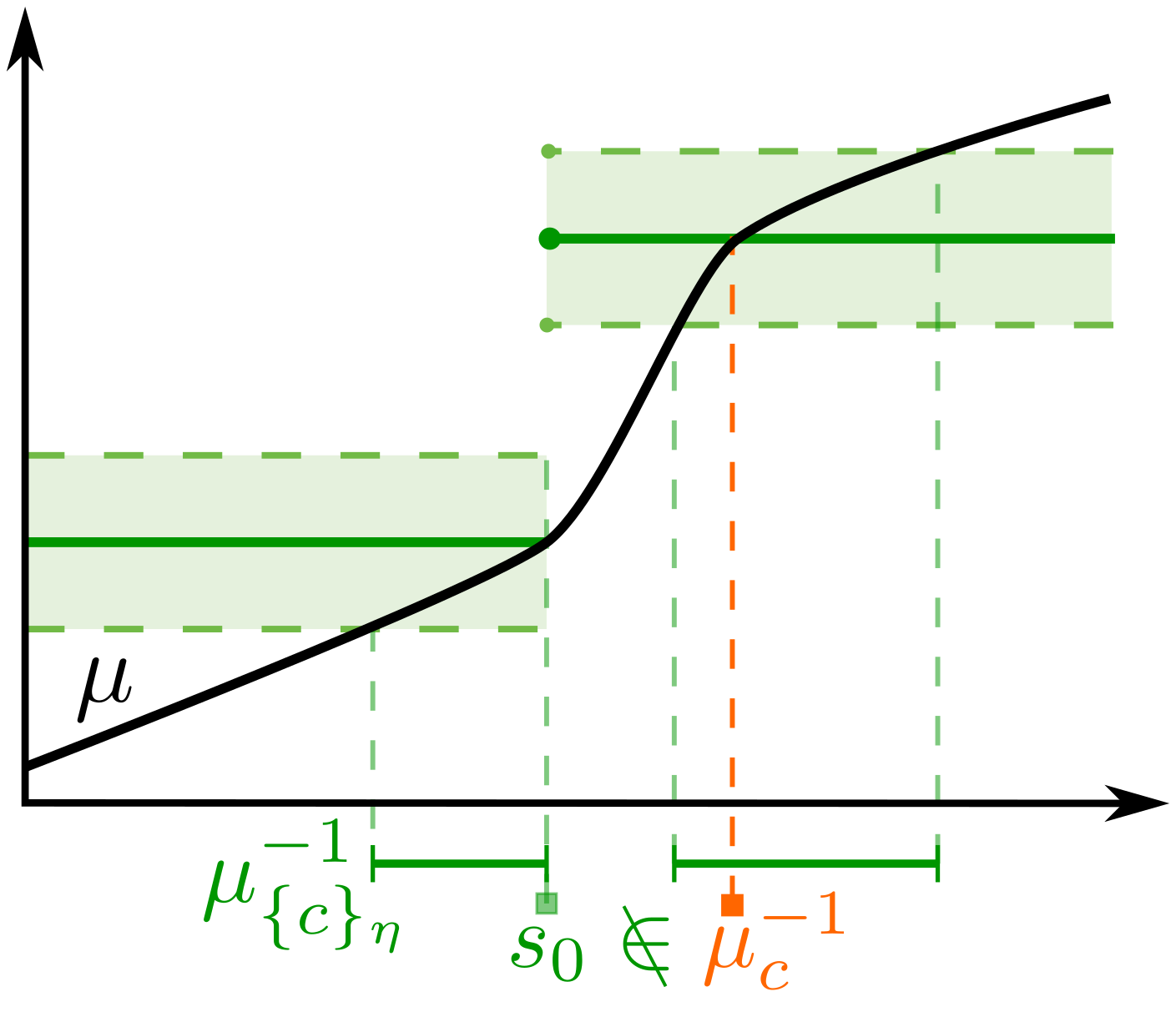
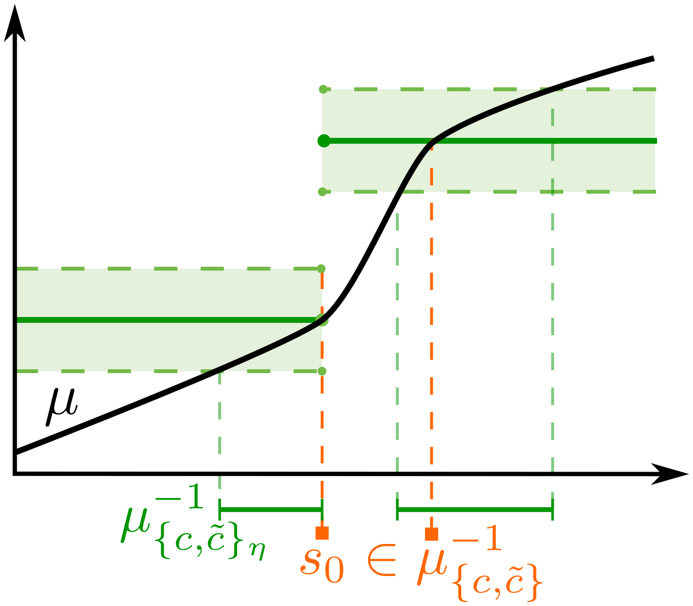
Figure 9: Illustration of the assumption that $\Gamma(\partial\mathcal{C})$ needs to be closed for Hausdorff convergence in Lemma 7. Left: Since $c$ is only right continuous at $s_{0}$ and $\mu(s_{0})$ is identical to the left sided limit of $c$ at $s_{0}$ the set ${\rm cl}\mu^{-1}_{c_{\eta}}$ does not converge in Hausdorff distance to $\mu^{-1}_{c}$. Right: If the set $\mathcal{C}$ is extended to include the function $\tilde{c}$ which is equal to $c$ for all $S\setminus\{s_{0}\}$ and $\tilde{c}(s_{0})$ is the left limit of $c$, then ${\rm cl}\mu^{-1}_{\{c,\tilde{c}\}_{\eta}}$ does converge to $\mu^{-1}_{\{c,\tilde{c}\}}$ in Hausdorff-distance.

Appendix D The Difference between $">"$ or $"\geq"$ Excursion Sets

This section explains why it is more natural to consider statements of the form $\hat{\mathcal{L}}_{c_{q}^{-}}\subseteq\mathcal{L}_{c^{-}}$ and $\hat{\mathcal{U}}_{c_{q}^{+}}\subseteq\mathcal{U}_{c^{+}}$ than the statements $S\setminus\hat{\mathcal{U}}_{c_{q}^{-}}\subseteq S\setminus\mathcal{U}_{c^{-}}$ and $S\setminus\hat{\mathcal{L}}_{c_{q}^{+}}\subseteq S\setminus\mathcal{L}_{c^{+}}$ which are used in the literature. For example, [43, 5, 6, 29] all use $S\setminus\hat{\mathcal{L}}_{c_{q}^{+}}\subseteq S\setminus\mathcal{L}_{c}\subseteq S\setminus\hat{\mathcal{L}}_{c_{q}^{-}}$ for $c^{\pm}=c$. The main issue with excursion sets using ”$\geq$” instead of ”$>$” is that a so called open ball condition is required to prove sharp upper bounds. This condition is restrictive since it means that $\mu$ cannot be flat on $\Gamma\big{(}\partial\mathcal{C}\big{)}$ as illustrated in Fig. 10. Because this section only serves an illustrative purpose, we simplify the proof by assuming $\mathfrak{u}^{-1}_{\mathcal{C}}=\mu^{-1}_{\mathcal{C}}$. This means that $\mu^{-1}_{\mathcal{C}}\subseteq S$ is closed. Furthermore, we require the following assumptions:

• There exist an $\tilde{\eta}>0$ such that the restriction of $G_{N}$ to $\mu^{-1}_{\mathcal{C}_{\tilde{\eta}}}$ has almost surely continuous sample paths.

• Assume that for all open $\mathcal{O}_{s}\subset S$ containing $s\in\mu^{-1}_{\partial\mathcal{C}^{-}}\cap\mu^{-1}_{\mathcal{C}^{-}}$ there is a $c^{-}\in\mathcal{C}^{-}$ such that $\mathcal{O}_{s}\cap\mathcal{U}_{c^{-}}\neq\emptyset$ and for all open $\mathcal{O}_{s}\subset S$ containing $s\in\mu^{-1}_{\partial\mathcal{C}^{+}}\cap\mu^{-1}_{\mathcal{C}^{+}}$ there is a $c^{+}\in\mathcal{C}^{+}$ such that $\mathcal{O}_{s}\cap\mathcal{L}_{c^{+}}\neq\emptyset$.

Remark 21.

Condition (A2’) is stronger than Condition (A2), since the latter only required continuity from outside $\mu^{-1}_{\mathcal{C}}$ towards $\mu^{-1}_{\partial\mathcal{C}}$ of $G_{N}$ while (A2’) requires additionally the continuity from the inside $\mu^{-1}_{\mathcal{C}}$ towards $\mu^{-1}_{\partial\mathcal{C}}$.

Remark 22.

If $\mathcal{C}=\{c\}$ for $c\in\mathcal{F}(S)$ then $\mu^{-1}_{\partial\mathcal{C}}=\mu^{-1}_{\mathcal{C}}=\big{\{}s\in S:~{}\mu(s)=c(s)\big{\}}$ and (A5) is equivalent to the open ball condition of Assumption 2.1.(a) from [43].

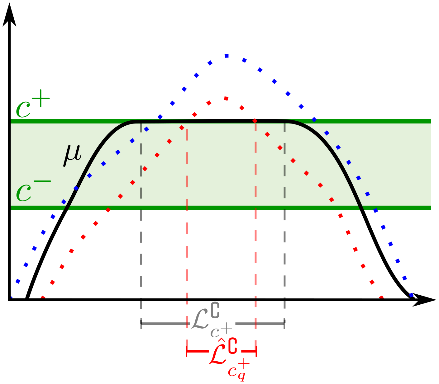
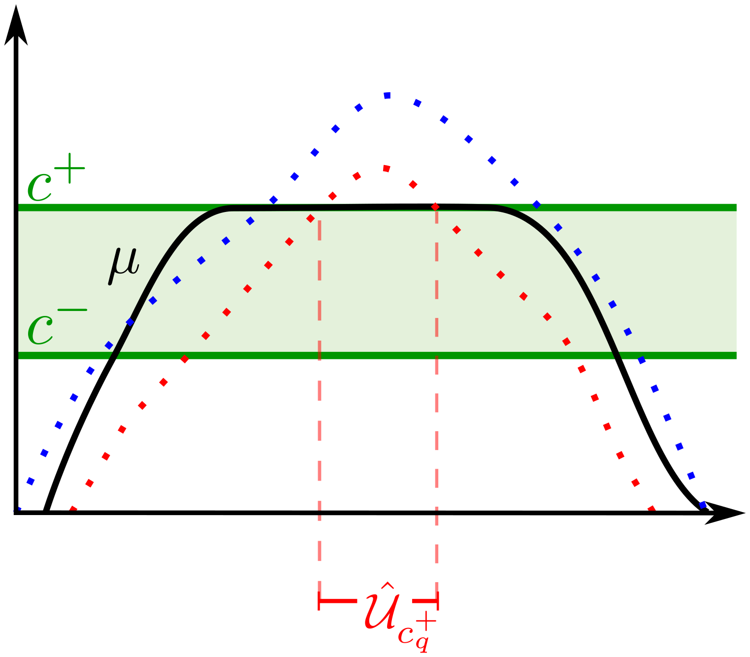
Figure 10: Illustration that the inclusion $S\setminus\hat{\mathcal{L}}_{c_{q}^{+}}\subseteq S\setminus\mathcal{L}_{c^{+}}$ requires more assumptions to obtain a sharp upper bound than $\hat{\mathcal{U}}_{c_{q}^{+}}\subseteq\mathcal{U}_{c^{+}}$. Condition (A5) excludes such cases with $\Gamma(\mu)$ and $\Gamma\big{(}\mathcal{C}^{\pm}\big{)}$ are tangential to each other on an open neighborhood of $S$. Left: the inclusion $S\setminus\hat{\mathcal{L}}_{c_{q}^{+}}\subseteq S\setminus\mathcal{L}_{c^{+}}$ does hold true although the band defined by $q$ does not contain $\mu$. Right: the problem is resolved because $\hat{\mathcal{U}}_{c_{q}^{+}}\not\subseteq\mathcal{U}_{c^{+}}=\emptyset$.

The following theorem shows that SCoPE sets using excursion sets with ”$\geq$” instead of ”$>$” require the stronger assumptions (A2’) and (A5) to obtain an upper bound.

Theorem 8.

Let $\mathcal{C}^{\pm}\subseteq\mathcal{F}(S)$ and assume (A1)-(A3) for $\mathcal{C}=\mathcal{C}^{-}\cup\mathcal{C}^{+}$. Define $c^{\pm q}=c^{\pm}\pm q\tau_{N}\sigma$. Then

$$\liminf_{N\rightarrow\infty}\mathbb{P}_{*}\left[\,\forall c^{-}\in\mathcal{C}^{-}\,\forall c^{+}\in\mathcal{C}^{+}:~{}\hat{\mathcal{U}}_{c_{q}^{-}}^{\complement}\subseteq\mathcal{U}_{c^{-}}^{\complement}~{}\wedge~{}\hat{\mathcal{L}}_{c_{q}^{+}}^{\complement}\subseteq\mathcal{L}_{c^{+}}^{\complement}\,\right]\geq\mathbb{P}\left[\,\mathfrak{T}_{\mathcal{C}^{-},\mathcal{C}^{+}}(G)<q\,\right]\,.$$

If also either $\mu^{-1}_{\partial\mathcal{C}}\cap\mu^{-1}_{\mathcal{C}}=\emptyset$ or else (A2’) and (A5), then

$$\limsup_{N\rightarrow\infty}\mathbb{P}_{*}\left[\,\forall c^{-}\in\mathcal{C}^{-}\,\forall c^{+}\in\mathcal{C}^{+}:~{}\hat{\mathcal{U}}_{c_{q}^{-}}^{\complement}\subseteq\mathcal{U}_{c^{-}}^{\complement}~{}\wedge~{}\hat{\mathcal{L}}_{c_{q}^{+}}^{\complement}\subseteq\mathcal{L}_{c^{+}}^{\complement}\,\right]\leq\mathbb{P}\left[\,\mathfrak{T}_{\mathcal{C}^{-},\mathcal{C}^{+}}(G)\leq q\,\right]\,.$$

Proof.

The proof of the lower bound follows along the lines of the proof given in Theorem 1. Therefore it is omitted. Only the upper bound requires a more complicated proof.

The idea is similar to the proof of the upper bound of the SCoPE Set Metatheorem 7. The only difference is that it is necessary to prove

$$\textbf{(E1)}~{}\forall c^{-}\in\mathcal{C}^{-}\,\forall c^{+}\in\mathcal{C}^{+}:~{}\big{\{}\hat{\mu}_{N}(s)+q\tau_{N}\sigma(s)\leq c^{-}(s)\big{\}}\subseteq\big{\{}\mu(s)\leq c^{-}(s)\big{\}}$$

$$\quad\quad\quad\quad\quad\quad\quad\quad\quad\quad\quad\wedge\big{\{}\hat{\mu}_{N}(s)-a\tau_{N}\sigma(s)\geq c^{+}(s)\big{\}}\subseteq\big{\{}\mu(s)\geq c^{+}(s)\big{\}}$$

$$\Longrightarrow{}{}{} \textbf{(E2)}~{}\forall s\in\mu^{-1}_{\mathcal{C}^{-}}\,\forall s^{\prime}\in\mu^{-1}_{\mathcal{C}^{+}}:~{}\hat{\mu}_{N}(s)-q\tau_{N}\sigma(s)\leq\mu(s)$$

$$\quad\quad\quad\quad\quad\quad\quad\quad\quad\quad\quad\quad\quad\quad\wedge~{}\mu(s^{\prime})\leq\hat{\mu}_{N}(s^{\prime})+q\tau_{N}\sigma(s^{\prime})$$

for the subset of $\Omega$ where $\hat{\mu}_{N}$ has continuous sample paths on $\mu^{-1}_{\mathcal{C}_{\tilde{\eta}}}$.

Assume (E1) holds, but not (E2). W.l.o.g. assume there exist an $s^{*}\in\mu^{-1}_{\mathcal{C}^{+}}$ such that $\hat{\mu}_{N}(s^{*})-q\tau_{N}\sigma(s^{*})\geq\mu(s^{*})$, i.e., $G_{N}(s^{*})\geq q$. First we assume $s^{*}\in\mu^{-1}_{\mathcal{C}^{+}}\setminus\mu^{-1}_{\partial\mathcal{C}^{+}}$. Since $\mu^{-1}_{\mathcal{C}^{+}}\setminus\mu^{-1}_{\partial\mathcal{C}^{+}}$ is open, there exists $c^{+}\in\mathcal{C}^{+}$ such that $c^{+}(s^{*})\in\big{(}\mu(s^{*}),\hat{\mu}_{N}(s^{*})-q\tau_{N}\sigma(s^{*})\big{)}$. Thus, $s^{*}\notin\mathcal{L}_{c^{+}}^{\complement}$, but $\hat{\mu}_{N}(s^{*})-q\tau_{N}\sigma(s^{*})\geq c^{+}(s^{*})$, which contradicts (E2). On the other hand, for $s^{*}\in\mu^{-1}_{\partial\mathcal{C}^{+}}\cap\mu^{-1}_{\mathcal{C}^{+}}$, choose $\mathcal{O}_{s^{*}}$ small enough such that $G_{N}(s)\geq q$ for all $s\in\mathcal{O}_{s^{*}}$. This is possible by (A2’). Then (A5) guarantees the existence of $c^{+}$ such that $s^{\prime}\in\mathcal{O}_{s^{*}}\cap\mathcal{L}_{c^{+}}$. Thus, $s^{\prime}\notin\mathcal{L}_{c^{+}}^{\complement}$, but $G_{N}(s^{\prime})\geq q$. A contradiction.

Similarly, the case $s^{*}\in\mu^{-1}_{\mathcal{C}^{-}}$ can be treated. Hence as in the proof of Theorem 7 an application of the Portmanteau Theorem finishes the proof. ∎

Appendix E Further Results on SCoPE sets for the Linear Model

In the main manuscript we derived asymptotic SCoPE sets over $\big{(}\{0\},\{0\})$ for the linear model. Here we derive further results.

E.1 Asymptotic SCoPE sets

The next theorems provide asymptotic SCoPE sets over $\big{(}\mathcal{C}^{-},\mathcal{C}^{+})$ with $\mathcal{C}^{-}=\{-\Delta\}$, $\mathcal{C}^{+}=\{\Delta\}$ and with $\mathcal{C}^{\pm}=\big{\{}\delta~{}|~{}\delta\in[-\Delta,\Delta]\big{\}}$ for the linear model. As usual, we identify a constant with the function being constant over $\mathbb{S}^{K-1}$. The proof is a simple application of Theorem 1, if one realizes that $\Delta\leq\|\bm{\beta}\|$ implies that $\big{\{}\bm{a}\in\mathbb{R}^{K}~{}|~{}\bm{a}^{T}\bm{\beta}=\Delta\big{\}}\cap\mathbb{S}^{K-1}\neq\emptyset$ and $\Delta>\|\bm{\beta}\|$ implies $\big{\{}\bm{a}\in\mathbb{R}^{K}~{}|~{}\bm{a}^{T}\bm{\beta}=\Delta\big{\}}\cap\mathbb{S}^{K-1}=\emptyset$.

Corollary 6.

Assume the setting of Corollary 5. Let $\Delta>0$ , $q\geq 0$ and $\bm{\varepsilon}\sim\mathcal{N}(0,I_{K\times K})$. If $\Delta\leq\|\bm{\beta}\|$, then

$$\begin{split}\lim_{N\rightarrow\infty}\mathbb{P}&\left[\,\hat{\mathcal{L}}_{-\Delta-\tau_{N}q\sigma}\subseteq\mathcal{L}_{\Delta}~{}\wedge~{}\hat{\mathcal{U}}_{\Delta+\tau_{N}q\sigma}\subseteq\mathcal{U}_{\Delta}\,\right]=\mathbb{P}\left[\,\|\bm{\varepsilon}\|\max_{\begin{subarray}{c}\|\mathfrak{X}^{-1/2}\bm{a}\|=1\\ \bm{a}^{T}\mathfrak{X}^{-1/2}\bm{\beta}=\Delta\end{subarray}}\frac{\bm{a}^{T}\bm{\varepsilon}}{\|\bm{a}\|\|\bm{\varepsilon}\|}\leq q\,\right]\,.\end{split}$$

If additionally $\mathfrak{X}=I_{K\times K}$, then

$$\begin{split}\lim_{N\rightarrow\infty}\mathbb{P}&\left[\,\hat{\mathcal{L}}_{-\Delta-\tau_{N}q\xi}\subseteq\mathcal{L}_{\Delta}~{}\wedge~{}\hat{\mathcal{U}}_{\Delta+\tau_{N}q\xi}\subseteq\mathcal{U}_{\Delta}\,\right]\\ &=\mathbb{P}\left[\,\frac{\Delta}{\|\bm{\beta}\|}\mathcal{N}(0,1)+\sqrt{1-\frac{\Delta^{2}}{\|\bm{\beta}\|^{2}}}\left\|\mathcal{N}\left(0,I_{(K-1)\times(K-1)}\right)\right\|\leq q\,\right]\,,\end{split}$$

where the two Gaussian random variables are independent of each other.

Otherwise, if $\Delta>\|\bm{\beta}\|$, then

$$\lim_{N\rightarrow\infty}\mathbb{P}\left[\,\hat{\mathcal{L}}_{-\Delta-\tau_{N}q\sigma}\subseteq\mathcal{L}_{\Delta}~{}\wedge~{}\hat{\mathcal{U}}_{\Delta+\tau_{N}q\sigma}\subseteq\mathcal{U}_{\Delta}\,\right]=1.$$

Proof.

We only need to determine the limit distribution, if $\Delta\leq\|\bm{\beta}\|$. Using Theorem 1 and simple algebra yields

$$\begin{split}\max\Bigg{(}\max_{\begin{subarray}{c}\|\bm{a}\|=1\\ \bm{a}^{T}\bm{\beta}=\Delta\end{subarray}}&\frac{\bm{a}^{T}\mathfrak{X}^{1/2}\bm{\varepsilon}}{\|\mathfrak{X}^{1/2}\bm{a}\|},\max_{\begin{subarray}{c}\|\bm{a}\|=1\\ \bm{a}^{T}\bm{\beta}=-\Delta\end{subarray}}\frac{-\bm{a}^{T}\mathfrak{X}^{1/2}\bm{\varepsilon}}{\|\mathfrak{X}^{1/2}\bm{a}\|}\Bigg{)}\\ &=\max\left(\max_{\begin{subarray}{c}\|\mathfrak{X}^{-1/2}\bm{a}\|=1\\ \bm{a}^{T}\mathfrak{X}^{-1/2}\bm{\beta}=\Delta\end{subarray}}\frac{\bm{a}^{T}\bm{\varepsilon}}{\|\bm{a}\|},\max_{\begin{subarray}{c}\|\mathfrak{X}^{-1/2}\bm{a}\|=1\\ \bm{a}^{T}\mathfrak{X}^{-1/2}\bm{\beta}=-\Delta\end{subarray}}\frac{-\bm{a}^{T}\bm{\varepsilon}}{\|\bm{a}\|}\right)\\ &=\max_{\begin{subarray}{c}\|\mathfrak{X}^{-1/2}\bm{a}\|=1\\ \bm{a}^{T}\mathfrak{X}^{-1/2}\bm{\beta}=\Delta\end{subarray}}\frac{\bm{a}^{T}\bm{\varepsilon}}{\|\bm{a}\|}\,.\end{split}$$

If additionally $\mathfrak{X}=I_{K\times K}$ we can simplify the limit distribution further using Lemma 9:

$$\begin{split}\max_{\begin{subarray}{c}\|\bm{a}\|=1\\ \bm{a}^{T}\bm{\beta}=\Delta\end{subarray}}\frac{\bm{a}^{T}\bm{\varepsilon}}{\|\bm{a}\|}&=\frac{\Delta}{\|\bm{\beta}\|}\frac{\bm{\beta}^{T}\bm{\varepsilon}}{\|\bm{\beta}\|}+\sqrt{1-\frac{\Delta^{2}}{\|\bm{\beta}\|^{2}}}\left\|P_{E}^{\bot}\bm{\varepsilon}\right\|\\ &=\frac{\Delta}{\|\bm{\beta}\|}\mathcal{N}(0,1)+\sqrt{1-\frac{\Delta^{2}}{\|\bm{\beta}\|^{2}}}\left\|\mathcal{N}\left(0,I_{(K-1)\times(K-1)}\right)\right\|\,,\end{split}$$

Here $P_{E}^{\bot}$ is the orthogonal projection onto the hyperplane $E=\{\bm{x}\in\mathbb{R}^{K}:~{}\bm{\beta}^{T}\bm{x}=0\}$ and the two Gaussian random variables are independent of each other. ∎

Remark 23.

The interpretation of this result is similar to the interpretation of Corollary 5. The difference is that it is designed to detect contrasts such that $|\bm{\beta}^{T}\bm{a}|>\Delta$ for some $\Delta>0$. The limiting process depends on the true $\bm{\beta}$ (in the case of $\mathfrak{X}=I_{K\times K}$ only on $\|\bm{\beta}\|$) and most importantly in the case $\|\bm{\beta}\|<\Delta$ the probability of detecting any contrast such that $|\bm{\beta}^{T}\bm{a}|>\Delta$ is asymptotically equal to zero.

Corollary 7.

Assume the setting of Corollary 5. Let $\Delta,q\geq 0$ and $\bm{\varepsilon}\sim\mathcal{N}(0,I_{K\times K})$. If $\Delta\leq\|\bm{\beta}\|$, then

$$\begin{split}\lim_{N\rightarrow\infty}\mathbb{P}\Bigg{[}\,\forall l\in[-\Delta,\Delta]:~{}&\hat{\mathcal{L}}_{-l-\tau_{N}q\sigma}\subseteq\mathcal{L}_{l}~{}\wedge~{}\hat{\mathcal{U}}_{l+\tau_{N}q\sigma}\subseteq\mathcal{U}_{l}\,\Bigg{]}\\ &=\mathbb{P}\Bigg{[}\,\|\bm{\varepsilon}\|\max_{l\in[-\Delta,\Delta]}\max_{\begin{subarray}{c}\|\mathfrak{X}^{-1/2}\bm{a}\|=1\\ \bm{a}^{T}\mathfrak{X}^{-1/2}\bm{\beta}=l\end{subarray}}\frac{\bm{a}^{T}\bm{\varepsilon}}{\|\bm{a}\|\|\bm{\varepsilon}\|}\leq q\,\Bigg{]}\,.\end{split}$$

If additionally $\mathfrak{X}=I_{K\times K}$, then

$$\begin{split}&\lim_{N\rightarrow\infty}\mathbb{P}\left[\,\forall l\in[-\Delta,\Delta]:~{}\hat{\mathcal{L}}_{-l-\tau_{N}q\xi}\subseteq\mathcal{L}_{l}~{}\wedge~{}\hat{\mathcal{U}}_{l+\tau_{N}q\xi}\subseteq\mathcal{U}_{l}\,\right]\\ &\hskip 56.9055pt=\mathbb{P}\Bigg{[}\,\mathds{1}_{\{\Delta\|\bm{\varepsilon}\|<\|\bm{\beta}\|\varepsilon_{1}\}}\left(\frac{\Delta}{\|\bm{\beta}\|}\varepsilon_{1}+\sqrt{1-\frac{\Delta^{2}}{\|\bm{\beta}\|^{2}}}\left\|(\varepsilon_{2},\ldots,\varepsilon_{K})\right\|\right)\\ &\hskip 256.0748pt+\mathds{1}_{\{\Delta\|\bm{\varepsilon}\|\geq|\bm{\beta}^{T}\bm{\varepsilon}|\}}\|\bm{\varepsilon}\|\leq q\,\Bigg{]}\,,\end{split}$$

where $\mathds{1}_{A}$ is one if $A$ is true and zero else.

Otherwise, if $\Delta>\|\bm{\beta}\|$, then

$$\lim_{N\rightarrow\infty}\mathbb{P}\left[\,\forall l\in[-\Delta,\Delta]:~{}\hat{\mathcal{L}}_{-l-\tau_{N}q\sigma}\subseteq\mathcal{L}_{l}~{}\wedge~{}\hat{\mathcal{U}}_{l+\tau_{N}q\sigma}\subseteq\mathcal{U}_{l}\,\right]=\chi^{2}\big{(}q^{2},K\big{)}.$$

Proof.

The limit distribution in the general case follows from Theorem 1 and simple algebra. In order to get the limit process for $\mathfrak{X}=I_{K\times K}$, recall that $P_{E}^{\bot}$ is the orthogonal projection onto the hyperplane $E=\{\bm{x}\in\mathbb{R}^{K}:~{}\bm{\beta}^{T}\bm{x}=0\}$. With this at hand and Lemma 9 we obtain

$$\begin{split}\max_{l\in[-\Delta,\Delta]}\max_{\begin{subarray}{c}\|\bm{a}\|=1\\ \bm{a}^{T}\bm{\beta}=l\end{subarray}}\frac{\bm{a}^{T}\bm{\varepsilon}}{\|\bm{a}\|\|\bm{\varepsilon}\|}&=\max_{\lambda\in[-\Delta/\|\bm{\beta}\|,\Delta/\|\bm{\beta}\|]}\lambda\frac{\bm{\beta}^{T}\bm{\varepsilon}}{\|\bm{\beta}\|}+\sqrt{1-\lambda^{2}}\left\|P_{E}^{\bot}\bm{\varepsilon}\right\|\\ &=\mathds{1}_{\{\Delta\|\bm{\varepsilon}\|<|\bm{\beta}^{T}\bm{\varepsilon}|\}}\left(\frac{\Delta}{\|\bm{\beta}\|}\frac{|\bm{\beta}^{T}\bm{\varepsilon}|}{\|\bm{\beta}\|}+\sqrt{1-\frac{\Delta^{2}}{\|\bm{\beta}\|^{2}}}\left\|P_{E}^{\bot}\bm{\varepsilon}\right\|\right)\\ &\hskip 170.71652pt+\mathds{1}_{\{\Delta\|\bm{\varepsilon}\|\geq|\bm{\beta}^{T}\bm{\varepsilon}|\}}\|\bm{\varepsilon}\|\,,\end{split}$$

where $\mathds{1}_{A}$ is one if $A$ is true and zero else. ∎

E.2 Multiple Linear Regression and Scheffé’s Test

Assume the simple multiple regression model, i.e.,

$$\begin{split}\bm{y}\sim\mathcal{N}\left(X\bm{\beta},\xi^{2}I_{N\times N}\right)\,,~{}X\in\mathbb{R}^{N\times K}\,,~{}\xi\in\mathbb{R}_{>0}\end{split}$$

such that $X$ has rank $K+1<N$. The BLUE of $\bm{\beta}$ is given by $\hat{\bm{\beta}}=(X^{T}X)^{-1}X^{T}\bm{y}$ and the variance $\xi^{2}$ of the error can be estimated by $s^{2}=\|\bm{y}-X\hat{\bm{\beta}}\|^{2}/(N-K-1)$.

In practice often not $\bm{\beta}$, but different linear contrasts $\bm{a}^{T}\bm{\beta}$, $\bm{a}\in\mathbb{R}^{K}$, are of interest. Interpreting $\bm{a}\in\mathbb{R}^{K}$ as the parameter set of a stochastic process, we can define the processes

$$\begin{split}\hat{\mu}(\bm{a})&=\bm{a}^{T}\hat{\bm{\beta}}\\ \hat{\sigma}^{2}(\bm{a})&=s^{2}\bm{a}^{T}\big{(}X^{T}X\big{)}^{-1}\bm{a}\,,\end{split}$$

which are the estimates of $\mu(\bm{a})=\bm{a}^{T}\bm{\beta}$ and the variance $\sigma^{2}(\bm{a})=s^{2}\bm{a}^{T}\big{(}X^{T}X\big{)}^{-1}\bm{a}$. Since all involved quantities are continuous in $\bm{a}$ we obtain the following Corollary of Proposition 1.

Proposition 3 (Scheffé Type CoPE Sets).

Assume the previously described multiple linear regression setting, then

$$\mathbb{P}\left[\forall c\in\mathcal{F}\big{(}\mathbb{R}^{K}\big{)}:~{}\hat{\mathcal{L}}_{c-q(K+1)\hat{\sigma}}\subseteq\mathcal{L}_{c}~{}\wedge~{}\hat{\mathcal{U}}_{c+q(K+1)\hat{\sigma}}\subseteq\mathcal{U}_{c}\,\right]=F\big{(}q^{2};K+1,N-K-1\big{)}\,.$$

Here $F\big{(}x;K+1,N-K-1\big{)}$ for $x\in\mathbb{R}$ denotes the cumulative distribution function of a $F_{K+1,N-K-1}$ distributed random variable.

Proof.

The proof is a simple consequence of Proposition 1 and [35, Theorem 8.5(i)], since

$$\begin{split}\mathbb{P}\left[\sup_{a\in\mathbb{R}^{K}}\left|\frac{\hat{\mu}(a)-\mu(a)}{\hat{\sigma}(a)}\right|\leq q\,\right]&=\mathbb{P}\left[\sup_{a\in\mathbb{R}^{K}}\frac{|\bm{a}^{T}(\hat{\bm{\beta}}-\bm{\beta})|^{2}}{s^{2}\bm{a}^{T}\big{(}X^{T}X\big{)}^{-1}\bm{a}(K+1)}\leq q^{2}\,\right]\\ &=F\big{(}q^{2};K+1,N-K-1\big{)}\,.\end{split}$$

∎

If $q\in\mathbb{R}$ is chosen such that $F\big{(}q^{2};K+1,N-K-1\big{)}=\alpha$ for some $\alpha\in(0,1)$, i.e., $q=\sqrt{F_{1-\alpha,K+1,N-K-1}}$, then the simultaneous Scheffé $(1-\alpha)$-confidence intervals are

$$\hat{\mu}(\bm{a})\pm q\hat{\sigma}(\bm{a})=\bm{a}^{T}\hat{\bm{\beta}}\pm s\sqrt{F_{1-\alpha,K+1,N-K-1}\bm{a}^{T}\big{(}X^{T}X\big{)}^{-1}\bm{a}(K+1)}\,,$$ (25)

compare [35, eq. (8.71)]. Therefore Proposition 3 explains the reason why testing $\mu(\bm{a})=0$ for all $\bm{a}\in\mathbb{R}^{K}$ using simultaneous Scheffé confidence intervals is not desirable to detect non-zero contrasts: the $\max$-statistic controls all possible inclusion statements, while valid simultaneous inference on the non-zero contrasts $\bm{a}\in\mathbb{R}^{K}$ requires only controlling the inclusions $\hat{\mathcal{L}}_{-q(K+1)\hat{\sigma}}\subseteq\mathcal{L}_{0}$ and $\hat{\mathcal{U}}_{q(K+1)\hat{\sigma}}\subseteq\mathcal{U}_{0}$. The latter can be targeted for example using Proposition 2.

Appendix F Exemplary Simulations of SCoPE sets for IID Observations

In this section we compare the SCoPE sets methodology in its simplest form which provides control over $\mathcal{C}^{\pm}=\{0\}$ to multiple testing strategies. We use the model discussed in Section 5.4 with $\bm{\sigma}\equiv 1$. We consider four difference models $A$, $B$, $C$ and $D$ which differ in the population means $\mu_{j}^{A}=0$, $j\in\{1,\ldots,80\}$,

$$\begin{split}\mu_{j}^{B}=\begin{cases}-0.3&\text{ for }j\in\{1,\ldots,30\}\\ 0&\text{ for }j\in\{31,\ldots,50\}\\ 0.2&\text{ for }j\in\{51,\ldots,80\}\end{cases}\,,\quad\quad\mu_{j}^{C}=\begin{cases}-0.3&\text{ for }j\in\{1,\ldots,5\}\\ 0&\text{ for }j\in\{6,\ldots,80\}\end{cases}\,,\end{split}$$

and $\mu^{C}_{j}=\sin\big{(}j/(2\pi)\big{)}$, $j\in\{1,\ldots,100\}$. Samples from these models are shown in Fig. 11.

The results deliver a simple message: SCoPE sets are at least as powerful and often more powerful than multiple testing procedures controlling the FWER while even offering information about the correct sign. The multiple testing procedures we compare to are Hommel’s procedure [22] which is based on the closure principle [28] and is to the best of our knowledge one of the most powerful strong $\alpha$-FWER tests for iid data and the Benjamini-Hochberg (BH) procedure which controls the false discovery rate. Of course, SCoPE sets cannot outperform the latter in terms of average true discoveries for small sample sizes since FDR targets a much looser error criterion which allows a higher number of false detection than the FWER. However, we included it to demonstrate that FDR control becomes for large sample sizes inferior to FWER control for discrete data as pointed out in Section 7.2 of the main manuscript. The latter can be best seen in the last three columns of Table 3 and Table 4.

Since $\bm{\mu}=0$ in Model A no true discoveries are possible. All methods except for using $\log(N)/10$ and $\log(N)/5$ converge quickly to the nominal coverage of $0.9$ compare Table 2. As we argued in Section 5.4 of the main manuscript a researcher would need to perform an insignificance analysis which means that many declared discoveries in the cases of SCoPE sets using $\log(N)/10$ and $\log(N)/5$ as the thickening factor for the estimator of Theorem 2 would be declared insignificant. Nevertheless, these choices are too small as can be seen also in Table 3 and Table 4. Remarkably, is that estimating the quantile using Storey’s trick, i.e., using $\hat{q}^{st}_{0.9}$, performs extremely well and converges quickly to the oracle values of average true and false discoveries. But even the very conservative choice of using a $0.9$-SCB to estimate the set $\hat{\mu}^{-1}_{0}$ is almost as good as Hommel’s procedure. Model D is a special case since it demonstrates the case that $\mu^{-1}_{0}=\emptyset$. The results can be found in Table 5. Here our oracle estimator does not provide good values for the simulated sample sizes since we correctly chose $q=0$. However, it is obvious that the probability of the containment of the upper and lower excursion sets slowly converges to one as predicted by the theory. Moreover, as argued in Section 7.2 the estimators do not suffer from this problem because the estimates of the quantile are usually not equal to zero.

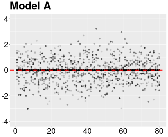
Figure 11: Illustration of samples of size $N=20$ from the multivariate Gaussian model introduced in Section 5.4 with the four different population mean functions from Section F.

	$N=20$			$N=50$			$N=100$			$N=200$			$N=500$			$N=1000$
Method	Cov	FD	TD	Cov	FD	TD	Cov	FD	TD	Cov	FD	TD	Cov	FD	TD	Cov	FD	TD
Oracle	90.7	0.10	-	89.8	0.11	-	89.7	0.11	-	90.5	0.10	-	89.7	0.11	-	89.7	0.11	-
$\hat{m}_{0}$	89.7	0.11	-	90.1	0.11	-	89.1	0.12	-	89.6	0.11	-	89.3	0.11	-	89.2	0.11	-
$\frac{\log(N)}{10}$	63.1	0.47	-	69.2	0.37	-	73.5	0.31	-	76.6	0.27	-	79.2	0.23	-	80.6	0.22	-
$\frac{\log(N)}{5}$	78.7	0.24	-	83.1	0.19	-	84.8	0.16	-	85.2	0.16	-	86.9	0.14	-	88.4	0.12	-
$\frac{\log(N)}{3}$	85.6	0.16	-	87.3	0.14	-	88.3	0.12	-	89.1	0.11	-	89.9	0.11	-	89.3	0.11	-
$\frac{\log(N)}{2}$	88.5	0.12	-	89.5	0.11	-	89.6	0.11	-	89.7	0.11	-	89.5	0.11	-	90.1	0.10	-
$0.9$-SCB	90.1	0.10	-	90.3	0.10	-	90.2	0.10	-	89.6	0.11	-	89.9	0.11	-	90.4	0.10	-
$0.1$-SCB	89.0	0.12	-	89.2	0.11	-	89.7	0.11	-	89.8	0.11	-	89.4	0.11	-	89.5	0.11	-
Hommel	-	0.10	-	-	0.10	-	-	0.10	-	-	0.10	-	-	0.10	-	-	0.10	-
BH	-	0.10	-	-	0.10	-	-	0.10	-	-	0.10	-	-	0.10	-	-	0.10	-

Table 2: Simulation results of Model $A$. The columns with title ”Cov” contain the empirical probability (in percentage) of the validity of the inclusions $\hat{\mathcal{L}}_{-q\hat{\sigma}/\sqrt{N}}\subseteq\mathcal{L}_{0}$ and $\hat{\mathcal{U}}_{q\hat{\sigma}/\sqrt{N}}\subseteq\mathcal{U}_{0}$. For the multiple testing methods Hommel and BH we do not report a ”Cov”-value since it is not their primary target and can only be derived through the error of the third kind. The columns with title ”FD” contain the average number of false discoveries and ”TD” contains the average number of true detection. Note that for SCoPE sets a false detection means making a directional error, i.e., an Type III error, or an Type I error, while for the multiple testing methods (Hommel, BH) a false detection only means making a Type I error.

	$N=20$			$N=50$			$N=100$			$N=200$			$N=500$			$N=1000$
Method	Cov	FD	TD	Cov	FD	TD	Cov	FD	TD	Cov	FD	TD	Cov	FD	TD	Cov	FD	TD
Oracle	89.9	0.10	2.4	89.9	0.11	9.1	89.8	0.11	22.9	90.1	0.10	42.8	89.7	0.11	58.5	89.9	0.11	60.0
$\hat{m}_{0}$	96.2	0.04	1.1	94.2	0.06	6.7	91.4	0.09	21.4	89.9	0.11	42.6	89.5	0.11	58.6	89.1	0.12	60.0
$\frac{\log(N)}{10}$	82.3	0.20	3.6	80.3	0.22	12.7	76.8	0.28	29.1	74.9	0.29	47.5	78.2	0.25	59.2	79.6	0.23	60.0
$\frac{\log(N)}{5}$	90.8	0.10	2.2	90.3	0.10	8.8	88.3	0.13	24.0	86.5	0.15	44.2	86.2	0.15	58.8	87.8	0.13	60.0
$\frac{\log(N)}{3}$	94.6	0.06	1.5	94.1	0.06	6.8	92.7	0.08	20.5	90.5	0.10	42.0	89.4	0.11	58.6	89.0	0.12	60.0
$\frac{\log(N)}{2}$	96.1	0.04	1.2	96.0	0.04	5.5	95.6	0.04	17.8	94.0	0.06	39.8	90.8	0.10	58.4	89.8	0.11	60.0
0.9-SCB	97.3	0.03	0.9	97.7	0.02	4.5	96.5	0.04	15.7	95.5	0.05	38.3	92.1	0.08	58.4	89.9	0.11	60.0
0.1-SCB	96.5	0.04	0.9	96.3	0.04	5.2	95.3	0.05	18.1	92.8	0.08	40.9	89.5	0.11	58.6	89.2	0.12	60.0
Hommel	-	0.03	0.8	-	0.03	4.5	-	0.04	16.5	-	0.06	39.5	-	0.10	58.4	-	0.10	60.0
BH	-	0.10	2.2	-	0.50	18.6	-	1.10	41.0	-	1.40	55.1	-	1.60	59.9	-	1.60	60.0

Table 3: Results of the simulation for Model $B$. The table has the same form as Table 2.

	$N=20$			$N=50$			$N=100$			$N=200$			$N=500$			$N=1000$
Method	Cov	FD	TD	Cov	FD	TD	Cov	FD	TD	Cov	FD	TD	Cov	FD	TD	Cov	FD	TD
Oracle	90.7	0.10	0.1	89.8	0.11	0.6	89.6	0.11	1.9	90.4	0.10	4.2	89.6	0.11	5.0	89.7	0.11	5.0
$\hat{m}_{0}$	90.0	0.11	0.1	90.4	0.10	0.6	89.3	0.11	2.0	89.8	0.11	4.2	89.6	0.11	5.0	89.3	0.11	5.0
$\frac{\log(N)}{10}$	63.8	0.46	0.3	69.4	0.36	1.1	73.4	0.31	2.6	76.5	0.27	4.5	79.2	0.23	5.0	80.7	0.22	5.0
$\frac{\log(N)}{5}$	79.2	0.23	0.2	83.2	0.19	0.8	84.9	0.16	2.2	85.3	0.16	4.3	86.8	0.14	5.0	88.3	0.12	5.0
$\frac{\log(N)}{3}$	86.1	0.15	0.1	87.4	0.13	0.7	88.5	0.12	2.0	89.1	0.11	4.2	89.9	0.11	5.0	89.3	0.11	5.0
$\frac{\log(N)}{2}$	88.9	0.12	0.1	89.7	0.11	0.6	89.8	0.11	2.0	89.7	0.11	4.2	89.6	0.11	5.0	90.1	0.10	5.0
0.9-SCB	90.7	0.10	0.1	90.8	0.10	0.6	90.5	0.10	1.9	89.6	0.11	4.2	89.9	0.11	5.0	90.4	0.10	5.0
0.1-SCB	89.5	0.11	0.1	89.6	0.11	0.6	89.9	0.11	2.0	89.7	0.11	4.2	89.4	0.11	5.0	89.6	0.11	5.0
Hommel	-	0.09	0.1	-	0.09	0.6	-	0.10	1.9	-	0.10	4.2	-	0.10	5.0	-	0.10	5.0
BH	-	0.10	0.1	-	0.20	0.8	-	0.40	2.6	-	0.60	4.7	-	0.60	5.0	-	0.60	5.0

Table 4: Results of the simulation for Model $C$. The table has the same form as Table 2.

	$N=20$			$N=50$			$N=100$			$N=200$			$N=500$			$N=1000$
Method	Cov	FD	TD	Cov	FD	TD	Cov	FD	TD	Cov	FD	TD	Cov	FD	TD	Cov	FD	TD
Oracle	0.1	5.96	94.0	1.3	3.71	96.3	4.7	2.55	97.5	12.1	1.77	98.2	28.2	1.07	98.9	42.6	0.72	99.3
$\hat{m}_{0}$	98.5	0.02	46.6	98.8	0.01	73.7	97.7	0.03	83.0	96.5	0.04	89.1	93.3	0.08	94.2	90.5	0.10	96.5
$\frac{\log(N)}{10}$	91.3	0.12	61.3	92.1	0.12	79.1	91.9	0.11	86.3	90.9	0.12	91.1	90.3	0.11	95.2	89.9	0.11	97.0
$\frac{\log(N)}{5}$	96.9	0.03	54.5	97.4	0.03	75.8	97.7	0.02	83.9	97.8	0.02	89.3	97.9	0.02	93.9	97.7	0.02	96.1
$\frac{\log(N)}{3}$	98.3	0.02	49.5	98.6	0.01	73.7	98.9	0.01	82.4	99.0	0.01	88.2	99.0	0.01	93.3	99.3	0.01	95.5
$\frac{\log(N)}{2}$	98.9	0.01	45.6	99.2	0.01	72.1	99.3	0.01	81.3	99.4	0.01	87.4	99.6	0.00	92.6	99.5	0.01	95.1
$0.9$-SCB	99.7	0.00	35.3	99.7	0.00	69.8	99.5	0.00	80.3	99.6	0.00	87.0	99.5	0.00	92.6	99.5	0.00	95.2
$0.1$-SCB	99.2	0.01	40.4	99.2	0.01	71.4	99.4	0.01	81.4	99.2	0.01	87.8	99.0	0.01	93.1	99.2	0.01	95.5
Hommel	-	-	38.1	-	-	70.6	-	-	80.9	-	-	87.5	-	-	93.0	-	-	95.5
BH	-	-	70.2	-	-	83.2	-	-	88.5	-	-	92.2	-	-	95.3	-	-	96.7

Table 5: Results of the simulation for Model $D$. The table has the same form as Table 2.

Appendix G Proofs of the Results in Section 3 and 4

G.1 Proof of Proposition 1

Proof.

The separability implies the measurability of the random variable

$$\sup_{s\in S}\left|\frac{\hat{\mu}(s)-\mu(s)}{\tau_{N}\hat{\sigma}(s)}\right|\,.$$

Hence the r.h.s. of the identity which we want to prove is well defined and it is enough to show that the equivalence of

$$\textbf{(E1)}~{}\forall s\in S:~{}\hat{\mu}(s)-q\tau_{N}\hat{\sigma}_{N}(s)\leq\mu(s)\leq\hat{\mu}(s)+q\tau_{N}\hat{\sigma}(s)$$

$$\textbf{(E2)}~{}\forall c^{-},c^{+}\in\mathcal{F}(S):~{}\hat{\mathcal{L}}_{c^{-}-q\tau_{N}\hat{\sigma}}\subseteq\mathcal{L}_{c^{-}}~{}\wedge~{}\hat{\mathcal{U}}_{c^{+}+q\tau_{N}\hat{\sigma}}\subseteq\mathcal{U}_{c^{+}}$$

Case (E1)$\Rightarrow$(E2): Assume that $s^{*}\in\hat{\mathcal{U}}_{c^{+}+q\tau_{N}\hat{\sigma}}$, i.e., $\hat{\mu}(s^{*})-q\tau_{N}\hat{\sigma}(s^{*})>c^{+}(s^{*})$. By (E1) it holds that $\mu(s^{*})\geq\hat{\mu}(s^{*})-q\tau_{N}\hat{\sigma}(s)$ which implies $\mu(s^{*})>c(s^{*})$, i.e., $s^{*}\in\hat{\mathcal{U}}_{c^{+}}$. Similar, $s^{*}\in\mathcal{L}_{c^{-}}$ combined with $\mu(s^{*})\leq\hat{\mu}(s^{*})+q\hat{\sigma}(s^{*})$ shows that $s^{*}\in\hat{\mathcal{L}}_{c^{-}-q\hat{\sigma}}$.
Case (E2)$\Rightarrow$(E1): By (E2) it holds that $\hat{\mathcal{U}}_{\mu+q\tau_{N}\hat{\sigma}}\subseteq\mathcal{U}_{\mu}=\emptyset$ and $S=\mathcal{L}_{\mu}^{\complement}\subseteq\hat{\mathcal{L}}_{\mu-q\tau_{N}\hat{\sigma}}^{\complement}$ which is equivalent to (E1). ∎

G.2 Proof of Theorem 1

Proof.

We want to apply the SCoPE Set Metatheorem 7 in the case that $q^{\pm}\equiv q$. By (A1)-(A3) we obtain from Lemma 6

$$\begin{split}T^{q,q}_{\mathcal{C}_{\eta_{N}}^{-},\mathcal{C}_{\eta_{N}}^{+}}(G_{N})\rightsquigarrow&\mathfrak{T}_{\mathcal{C}^{-},\mathcal{C}^{+}}(G)-q\,,\quad T^{q,q}_{\mathcal{C}^{-},\mathcal{C}^{+}}(G_{N})\rightsquigarrow T^{q,q}_{\mathcal{\mathcal{C}^{-}},\mathcal{C}^{+}}(G)\\ &T^{q,q}_{\mathcal{C}_{\tilde{\eta}}^{-},\mathcal{C}_{\tilde{\eta}}^{+}}(G_{N})\rightsquigarrow T^{q,q}_{\mathcal{C}_{\tilde{\eta}}^{-},\mathcal{C}_{\tilde{\eta}}^{+}}(G)\,.\end{split}$$

Therefore (M1) is satisfied. Condition (M2) holds since the random variable $T^{q,q}_{\mathcal{C}_{\tilde{\eta}}^{-},\mathcal{C}_{\tilde{\eta}}^{+}}(G)$ on $\mathbb{R}$ is tight which is equivalent to $T^{q,q}_{\mathcal{C}_{\tilde{\eta}}^{-},\mathcal{C}_{\tilde{\eta}}^{+}}(G_{N})$ being asymptotically tight [50, Lemma 1.3.8 ]. Assumption (M3) is part of Assumption (A1). ∎

G.3 Proof of Theorem 2

We first establish that the estimate $\hat{\mathfrak{u}}_{\mathcal{C}}^{-1}$ is with inner probability tending to one inside the set ${\rm cl}\,\mu^{-1}_{\mathcal{C}_{\tilde{\eta}}}$.

Lemma 8.

Assume $\hat{\mu}_{N}$ satisfies Definition 8(ii) for some $\tilde{\eta}>0$. Let $(k_{N})_{N\in\mathbb{N}}$ be a positive sequence such that $\lim_{N\rightarrow\infty}k_{N}\tau_{N}=0$. Then

$$\liminf_{N\rightarrow\infty}\mathbb{P}_{*}\Big{[}\,\hat{\mathfrak{u}}_{\pm\mathcal{C}}^{-1}\subseteq{\rm cl}\,\mu^{-1}_{\mathcal{C}_{\tilde{\eta}}}\,\Big{]}=\liminf_{N\rightarrow\infty}\mathbb{P}_{*}\Big{[}\,\hat{\mathfrak{u}}_{\mathcal{C}}^{-1}\subseteq{\rm cl}\,\mu^{-1}_{\mathcal{C}_{\tilde{\eta}}}\,\Big{]}=1\,.$$

Proof.

We prove that

$$\liminf_{N\rightarrow\infty}\mathbb{P}_{*}\Big{[}\,\hat{\mathfrak{u}}_{\mathcal{C}}^{-1}\subseteq{\rm cl}\,\mu^{-1}_{\mathcal{C}_{\tilde{\eta}}}\,\Big{]}=1$$ (26)

since it implies the other statement. Define ${\rm sgn}_{c,f}(s)={\rm sgn}\big{(}\,f(s)-c(s)\,\big{)}$ for $f\in\mathcal{F}(S)$ and the set

$$\hat{\mu}_{\mathcal{C}}^{-1}=\Big{\{}s\in S~{}\big{|}~{}\exists c\in\mathcal{C}:~{}|\,\hat{\mu}_{N}(s)-c(s)\,|\leq k_{N}\tau_{N}\sigma(s)\Big{\}}\subseteq\hat{\mathfrak{u}}_{\mathcal{C}}^{-1}\,.$$ (27)

Assume that $s\in\hat{\mu}_{\mathcal{C}}^{-1}\cap\big{(}S\setminus\mu^{-1}_{\mathcal{C}_{\tilde{\eta}}}\big{)}$. From Definition 8(ii) and (10) we obtain

$$\begin{split}\mathfrak{o}\big{(}\,K+Z_{N}(s)\,\big{)}\leq{\rm sgn}_{c,\mu}(s){\rm sgn}_{c,\hat{\mu}_{N}}(s)|\,\hat{\mu}_{N}(s)-c(s)\,|\leq{\rm sgn}_{c,\mu}(s){\rm sgn}_{c,\hat{\mu}_{N}}(s)k_{N}\tau_{N}\mathfrak{O}\end{split}$$

If ${\rm sgn}_{c,\mu}(s)={\rm sgn}_{c,\hat{\mu}_{N}}(s)$, this implies $Z_{N}(s)\leq\tau_{N}k_{N}\mathfrak{O}\mathfrak{o}^{-1}-K$. Since $\lim\tau_{N}k_{N}=0$ and $\inf_{s\in S}\tau_{N}^{-1}Z_{N}(s)$ is asymptotically tight it holds that

$$\limsup_{N\rightarrow\infty}\mathbb{P}^{*}\left[\,Z_{N}(s)\leq\tau_{N}k_{N}\mathfrak{O}\mathfrak{o}^{-1}-K\,\right]=\limsup_{N\rightarrow\infty}\mathbb{P}^{*}\Bigg{[}\,\frac{Z_{N}(s)}{\tau_{N}}\leq\frac{\tau_{N}k_{N}\mathfrak{O}\mathfrak{o}^{-1}-K}{\tau_{N}}\,\Bigg{]}=0$$

combining this with Remark 3 shows that

$$\begin{split}\limsup_{N\rightarrow\infty}\mathbb{P}^{*}\Big{[}\,\hat{\mu}_{\mathcal{C}}^{-1}\cap\big{(}S\setminus\mu^{-1}_{\mathcal{C}_{\tilde{\eta}}}\big{)}\neq\emptyset\,\Big{]}=0&~{}~{}\Leftrightarrow~{}~{}\liminf_{N\rightarrow\infty}\mathbb{P}_{*}\Big{[}\,\hat{\mu}_{\mathcal{C}}^{-1}\subseteq\mu^{-1}_{\mathcal{C}_{\tilde{\eta}}}\,\Big{]}=1\\ &~{}~{}\Leftrightarrow~{}~{}\liminf_{N\rightarrow\infty}\mathbb{P}_{*}\Big{[}\,\hat{\mathfrak{u}}_{\mathcal{C}}^{-1}\subseteq{\rm cl}\,\mu^{-1}_{\mathcal{C}_{\tilde{\eta}}}\,\Big{]}=1\end{split}$$

which is the claim. ∎

Using the above Lemma we can prove Theorem 2. The proof follows the idea of the proof of Theorem 3.6 from [11], yet it is more involved since it is significantly more general.

Proof.

We begin with proving the Hausdorff convergence of the estimator of $\mathfrak{u}^{-1}_{\mathcal{C}}$. To begin with let $\eta_{N}=\rho\mathfrak{o}k_{N}\tau_{N}$ for some $\rho\in(0,1)$ and recall the definition of $\hat{\mu}_{\mathcal{C}}^{-1}$ from (27). Assuming $N$ large enough such that $\eta_{N}<\tilde{\eta}$ we obtain

$$\begin{split}\mathbb{P}_{*}\Big{[}\,\mu^{-1}_{\mathcal{C}_{\eta_{N}}}\subseteq\hat{\mu}_{\mathcal{C}}^{-1}\,\Big{]}&=\mathbb{P}_{*}\Bigg{[}\,\sup_{s\in\mu^{-1}_{\mathcal{C}_{\eta_{N}}}}\inf_{c\in\mathcal{C}}\frac{|\hat{\mu}_{N}(s)-c(s)|}{\sigma(s)}\leq k_{N}\tau_{N}\,\Bigg{]}\\ &\geq\mathbb{P}_{*}\Bigg{[}\,\sup_{s\in\mu^{-1}_{\mathcal{C}_{\eta_{N}}}}\inf_{c\in\mathcal{C}}\frac{|\hat{\mu}_{N}(s)-\mu(s)|}{\sigma(s)}+\frac{|\mu(s)-c(s)|}{\sigma(s)}\leq k_{N}\tau_{N}\,\Bigg{]}\\ &\geq\mathbb{P}_{*}\Bigg{[}\,\sup_{s\in\mu^{-1}_{\mathcal{C}_{\eta_{N}}}}\inf_{c\in\mathcal{C}}\frac{|\hat{\mu}_{N}(s)-\mu(s)|}{\sigma(s)}+\rho k_{N}\tau_{N}\leq k_{N}\tau_{N}\,\Bigg{]}\\ &=\mathbb{P}_{*}\Bigg{[}\,\sup_{s\in\mu^{-1}_{\mathcal{C}_{\eta_{N}}}}|G_{N}(s)|\leq k_{N}(1-\rho)\,\Bigg{]}\\ &\geq\mathbb{P}_{*}\Bigg{[}\,\sup_{s\in{\rm cl}\,\mu^{-1}_{\mathcal{C}_{\tilde{\eta}}}}|G_{N}(s)|\leq k_{N}(1-\rho)\,\Bigg{]}\,.\end{split}$$

The latter converges to one since $\sup_{s\in{\rm cl}\,\mu^{-1}_{\mathcal{C}_{\tilde{\eta}}}}|G_{N}(s)|$ is asymptotically tight. Therefore we have $\liminf_{N\rightarrow\infty}\mathbb{P}_{*}\big{[}\,{\rm cl}\,\mu^{-1}_{\mathcal{C}_{\eta_{N}}}\subseteq\hat{\mathfrak{u}}_{\mathcal{C}}^{-1}\,\big{]}=1$ and thus

$$\begin{split}\limsup_{N\rightarrow\infty}\mathbb{P}^{*}\Bigg{[}\sup_{s\in\mathfrak{u}^{-1}_{\mathcal{C}}}\inf_{s^{\prime}\in\hat{\mathfrak{u}}_{\mathcal{C}}^{-1}}|s-s^{\prime}|>\epsilon\Bigg{]}\leq\limsup_{N\rightarrow\infty}\mathbb{P}^{*}\Bigg{[}\sup_{s\in{\rm cl}\,\mu^{-1}_{\mathcal{C}_{\eta_{N}}}}\inf_{s^{\prime}\in\hat{\mathfrak{u}}_{\mathcal{C}}^{-1}}|s-s^{\prime}|>\epsilon\Bigg{]}=0\,.\end{split}$$

Essentially the identical argument proves

$$\liminf_{N\rightarrow\infty}\mathbb{P}_{*}\Big{[}\mathfrak{u}^{-1}_{\pm\mathcal{C}}\subseteq\hat{\mathfrak{u}}_{\pm\mathcal{C}}^{-1}\Big{]}=1\,.$$ (28)

It remains to prove that

$$\begin{split}\limsup_{N\rightarrow\infty}\mathbb{P}^{*}\Bigg{[}\sup_{s\in\hat{\mathfrak{u}}_{\mathcal{C}}^{-1}}\inf_{s^{\prime}\in\mathfrak{u}^{-1}_{\mathcal{C}}}|s-s^{\prime}|>\epsilon\Bigg{]}=0\,.\end{split}$$ (29)

and under the continuity condition on $\mu$ that

$$\begin{split}\limsup_{N\rightarrow\infty}\mathbb{P}^{*}\Bigg{[}\sup_{s\in\hat{\mathfrak{u}}_{\pm\mathcal{C}}^{-1}}\inf_{s^{\prime}\in\mathfrak{u}^{-1}_{\pm\mathcal{C}}}|s-s^{\prime}|>\epsilon\Bigg{]}=0\,.\end{split}$$ (30)

To see the first statement note that whenever $\hat{\mathfrak{u}}_{\mathcal{C}}^{-1}\subseteq{\rm cl}\,\mu^{-1}_{\mathcal{C}_{\tilde{\eta}}}$ it holds that

$$\begin{split}\sup_{s\in\hat{\mu}_{\mathcal{C}}^{-1}}\inf_{c\in\mathcal{C}}|\mu(s)-c(s)|&\leq\sup_{s\in\hat{\mu}_{\mathcal{C}}^{-1}}\inf_{c\in\mathcal{C}}|\mu(s)-\hat{\mu}_{N}(s)|+|\hat{\mu}_{N}(s)-c(s)|\\ &\leq\sup_{s\in\hat{\mu}_{\mathcal{C}}^{-1}}|\mu(s)-\hat{\mu}_{N}(s)|+k_{N}\tau_{N}\mathfrak{O}\\ &\leq\sup_{s\in{\rm cl}\,\mu^{-1}_{\mathcal{C}_{\tilde{\eta}}}}|\mu(s)-\hat{\mu}_{N}(s)|+k_{N}\tau_{N}\mathfrak{O}\end{split}$$

which implies by Lemma 8 that

$$\begin{split}\liminf_{N\rightarrow\infty}\mathbb{P}_{*}\Bigg{[}&\sup_{s\in\hat{\mu}_{\mathcal{C}}^{-1}}\inf_{c\in\mathcal{C}}|\mu(s)-c(s)|\leq 2k_{N}\tau_{N}\mathfrak{O}\Bigg{]}\\ &\geq\liminf_{N\rightarrow\infty}\mathbb{P}_{*}\Bigg{[}\sup_{s\in{\rm cl}\,\mu^{-1}_{\mathcal{C}_{\tilde{\eta}}}}|\mu(s)-\hat{\mu}_{N}(s)|\leq k_{N}\tau_{N}\mathfrak{O}\Bigg{]}\\ &\geq\liminf_{N\rightarrow\infty}\mathbb{P}_{*}\Bigg{[}\sup_{s\in\mu^{-1}_{\mathcal{C}_{\tilde{\eta}}}}|G_{N}(s)|\leq k_{N}\Bigg{]}=1\,.\end{split}$$

and thus $\sup_{s\in\hat{\mu}_{\mathcal{C}}^{-1}}\inf_{c\in\mathcal{C}}|\mu(s)-c(s)|$ converges to zero outer almost surely. The latter implies $\sup_{s^{\prime}\in\hat{\mathfrak{u}}_{\mathcal{C}}^{-1}}\inf_{s\in\mathfrak{u}^{-1}_{\mathcal{C}}}|s-s^{\prime}|\rightarrow 0$ outer almost surely, which by Lemma 1.9.2 from [50] would finish the proof.

Let us assume that $\sup_{s\in\hat{\mu}_{\mathcal{C}}^{-1}}\inf_{c\in\mathcal{C}}|\mu(s)-c(s)|$ converges to zero outer almost surely. By Egorov’s Theorem (Lemma 1.9.2(iii) from [50]) this is equivalent to

$$\begin{split}\forall\delta>0\,\exists A\subseteq\Omega\,\forall\varepsilon>0\,&\forall\omega\in A\,\exists N^{\prime}\,\forall N>N^{\prime}:\\ &\mathbb{P}(A)\geq 1-\delta~{}\wedge~{}\sup_{s\in\hat{\mu}_{\mathcal{C}}^{-1}(\omega)}\inf_{c\in\mathcal{C}}|\mu(s)-c(s)|<\epsilon\end{split}$$ (31)

and assume that $\sup_{s^{\prime}\in\hat{\mathfrak{u}}_{\mathcal{C}}^{-1}}\inf_{s\in\mathfrak{u}^{-1}_{\mathcal{C}}}|s-s^{\prime}|\rightarrow 0$ is not converging outer almost surely, i.e.,

$$\begin{split}\exists\delta>0\,\forall A\subseteq\Omega\,\exists\varepsilon_{0}>0\,&\exists\omega_{0}\in A\,\forall N^{\prime}\,\exists N>N^{\prime}:\\ &\mathbb{P}(A)\geq 1-\delta~{}\wedge~{}\sup_{s^{\prime}\in\hat{\mathfrak{u}}_{\mathcal{C}}^{-1}(\omega_{0})}\inf_{s\in\mathfrak{u}^{-1}_{\mathcal{C}}}|s-s^{\prime}|\geq\epsilon_{0}\,.\end{split}$$ (32)

Here and latter for convenience we explicitly indicated where the dependence on $\omega/\omega_{0}$ is.

Let $\delta$ from (32). For this $\delta$ we choose the corresponding $A$ from (31). Hence by (32) there is a $\varepsilon_{0}$ and $\omega_{0}\in A$ such that

$$\sup_{s^{\prime}\in\hat{\mathfrak{u}}_{\mathcal{C}}^{-1}(\omega_{0})}\inf_{s\in\mathfrak{u}^{-1}_{\mathcal{C}}}|s-s^{\prime}|\geq\epsilon_{0}$$ (33)

We will now construct a contradiction between (31) and (32).

From 34 we obtain a sequence $(s_{N})_{N\in\mathbb{N}}\subset\hat{\mathfrak{u}}_{\mathcal{C}}^{-1}(\omega_{0})$ such that

$$\inf_{s\in\mathfrak{u}^{-1}_{\mathcal{C}}}|s-s_{N}|\geq\epsilon_{0}$$ (34)

for all $N>N^{\prime}$. By replacing $(s_{N})_{N\in\mathbb{N}}$ by a convergent subsequence since $S$ is compact we can w.l.o.g. assume that $s_{N}\rightarrow s^{*}$ for $N\rightarrow\infty$ with

$$s^{*}\in\bigcap_{N>N^{\prime}}\hat{\mathfrak{u}}_{\mathcal{C}}^{-1}(\omega_{0})=\bigcap_{N>N^{\prime}}{\rm cl}\hat{\mu}_{\mathcal{C}}^{-1}(\omega_{0})$$

and therefore

$$\inf_{s\in\mathfrak{u}^{-1}_{\mathcal{C}}}|s-s^{*}|\geq\epsilon_{0}$$ (35)

If $s^{*}\in\hat{\mu}^{-1}_{\mathcal{C}}(\omega_{0})$ for all $N>N^{\prime}$, then by (31) we have that $s^{*}\in\mu^{-1}_{\mathcal{C}}$ which contradicts (35). More general, if $s^{*}\in{\rm cl}\hat{\mu}^{-1}_{\mathcal{C}}(\omega_{0})=\hat{\mathfrak{u}}_{\mathcal{C}}^{-1}(\omega_{0})$ for all $N>N^{\prime}$ we find a sequence $(t_{N})_{N\in\mathbb{N}}$ such that $t_{N}\in\hat{\mu}^{-1}_{\mathcal{C}}(\omega_{0})$ converging to $s^{*}$. By (31) this means that $s^{*}\in\mathfrak{u}_{\mathcal{C}}^{-1}$ contradicting (35).

The same proof can be used to prove (30). The argument only breaks down in the last step. It does not follow in general from (31) that $s^{*}\in\mathfrak{u}_{\pm\mathcal{C}}^{-1}$, since it matters with which sign $\mu(t_{N})-c(t_{N})$ has. Under the continuity condition and the closedness of $\Gamma(\mathcal{C})$ it follows from (31) and the reasoning in the end of the proof of Lemma 7 that $s^{*}\in\mu^{-1}_{\mathcal{C}}\subset\mathfrak{u}_{\pm\mathcal{C}}^{-1}$.

∎

Appendix H Proofs of the Results in Section 5

The proofs of this section are based on the following lemma.

Lemma 9.

Let $l\in\mathbb{R}$, $\bm{a},\bm{w}\in\mathbb{R}^{K}$ and $\tfrac{l^{2}}{\|a\|^{2}}\leq 1$. Let $P=\big{(}\bm{v}_{1}^{T},\ldots,\bm{v}_{k-1}^{T}\big{)}\in\mathbb{R}^{K-1\times K}$, where $\bm{v}_{1},\ldots,\bm{v}_{K-1}$ form a basis of the hyperplane $E=\{\bm{x}\in\mathbb{R}^{K}:~{}\bm{a}^{T}\bm{x}=0\}$. Let $P_{E}^{\bot}=P(P^{T}P)^{-1}P^{T}$ the orthogonal projection onto $E$.

$$\begin{split}a)&~{}~{}~{}\max_{\begin{subarray}{c}\|\bm{x}\|=1\\ \bm{a}^{T}\bm{x}=l\end{subarray}}\pm\bm{x}^{T}\bm{w}=\pm l\frac{\bm{a}^{T}\bm{w}}{\|\bm{a}\|^{2}}+\sqrt{1-\tfrac{l^{2}}{\|\bm{a}\|^{2}}}\big{\|}P_{E}^{\bot}\bm{w}\big{\|}\\ b)&~{}~{}~{}\max_{\begin{subarray}{c}\|\bm{x}\|=1\\ \bm{a}^{T}\bm{x}=l\end{subarray}}|\bm{x}^{T}\bm{w}|=\left|l\frac{\bm{a}^{T}\bm{w}}{\|\bm{a}\|^{2}}\right|+\sqrt{1-\tfrac{l^{2}}{\|\bm{a}\|^{2}}}\big{\|}P_{E}^{\bot}\bm{w}\big{\|}\end{split}$$

Proof.

For $\bm{x}\in\mathbb{R}^{K}$ we define $\hat{\bm{x}}=\bm{x}/\|\bm{x}\|$. Every $\bm{x}\in\{\bm{x}\in\mathbb{R}^{K}:~{}\bm{a}^{T}\bm{x}=l\}$ can be decomposed into

$$\bm{x}=l\frac{\bm{a}}{\|\bm{a}\|^{2}}+\bm{x}_{E}\,,~{}~{}\text{with }\bm{x}_{E}\in E\,.$$

Using this decomposition, the fact that $\hat{\bm{x}}_{E}^{T}\bm{w}$ does not depend on $\|\bm{x}_{E}\|$ and that the smallest angle between the vector $\pm\bm{w}$ and the linear subspace $E$ is the angle between $\bm{w}$ and its orthogonal projection $P_{E}^{\bot}(\pm\bm{w})$ onto $E$, we obtain

$$\begin{split}\max_{\begin{subarray}{c}\|\bm{x}\|=1\\ \bm{a}^{T}\bm{x}=l\end{subarray}}\bm{x}^{T}(\pm\bm{w})&=\max_{\|\bm{x}_{E}\|^{2}=1-\tfrac{l^{2}}{\|\bm{a}\|^{2}}}\pm l\frac{\bm{a}^{T}\bm{w}}{\|\bm{a}\|^{2}}+\bm{x}_{E}^{T}(\pm\bm{w})\\ &=\pm l\frac{\bm{a}^{T}\bm{w}}{\|\bm{a}\|^{2}}+\max_{\|\bm{x}_{E}\|^{2}=1-\tfrac{l^{2}}{\|\bm{a}\|^{2}}}\|\bm{x}_{E}\|\hat{\bm{x}}_{E}^{T}(\pm\bm{w})\\ &=\pm l\frac{\bm{a}^{T}\bm{w}}{\|\bm{a}\|^{2}}+\sqrt{1-\tfrac{l^{2}}{\|\bm{a}\|^{2}}}\max_{\|\hat{\bm{x}}_{E}\|^{2}=1}\hat{\bm{x}}_{E}^{T}(\pm\bm{w})\\ &=\pm l\frac{\bm{a}^{T}\bm{w}}{\|\bm{a}\|^{2}}+\sqrt{1-\tfrac{l^{2}}{\|\bm{a}\|^{2}}}\frac{\bm{w}^{T}P_{E}^{\bot}}{\big{\|}P_{E}^{\bot}\bm{w}\big{\|}}\bm{w}\\ &=\pm l\frac{\bm{a}^{T}\bm{w}}{\|\bm{a}\|^{2}}+\sqrt{1-\tfrac{l^{2}}{\|\bm{a}\|^{2}}}\big{\|}P_{E}^{\bot}\bm{w}\big{\|}\,.\end{split}$$

This proves equation a). Finally, $b)$ is an immediate consequence of $a)$. ∎

H.1 Proof of Corollary 5

Proof.

Assumptions (A1)-(A4) are trivially satisfied in this setup, since $\mathbb{S}^{K-1}$ is compact, $\mu$ and $c$ continuous and $G_{N}$ defined in (13) has continuous sample paths. Let $\bm{\varepsilon}\sim\mathcal{N}(0,I_{K\times K})$. Applying Theorem 1 and Lemma 9 yields

$$\begin{split}\lim_{N\rightarrow\infty}\mathbb{P}\Big{[}\,\hat{\mathcal{U}}_{\tau_{N}q\sigma}\subseteq\mathcal{U}_{0}~{}\wedge~{}\hat{\mathcal{L}}_{-\tau_{N}q\sigma}\subseteq\mathcal{L}_{0}\,\Big{]}&=\mathbb{P}\Bigg{[}~{}\max_{\begin{subarray}{c}\|\bm{a}\|=1\\ \bm{a}^{T}\bm{\beta}=0\end{subarray}}\Bigg{|}\frac{\bm{a}^{T}\mathfrak{X}^{1/2}\bm{\varepsilon}}{\sqrt{\bm{a}^{T}\mathfrak{X}\bm{a}}}\Bigg{|}\leq q~{}\Bigg{]}\\ &=\mathbb{P}\Big{[}~{}\left\|P(P^{T}P)^{-1}P^{T}\bm{\varepsilon}\right\|\leq q~{}\Big{]}\,.\end{split}$$

If $\bm{\beta}\neq 0$ the matrix $P\in\mathbb{R}^{K\times(K-1)}$ is a matrix having a basis of the hyperplane $\big{\{}\bm{a}\in\mathbb{R}^{K}:~{}(\mathfrak{X}^{-1/2}\bm{\beta})^{T}\bm{a}=0\big{\}}$ as its columns, else $P=I_{K\times K}$. The claim follows since $P(P^{T}P)^{-1}P^{T}$ is an orthogonal projection and therefore

$$P(P^{T}P)^{-1}P^{T}\bm{\varepsilon}\sim\mathcal{N}\big{(}0,I_{(K-1+\mathds{1}_{\bm{\beta}=0})\times(K-1+\mathds{1}_{\bm{\beta}=0})}\big{)}\,.$$

∎

Appendix I Proofs of the Results in Section 6

I.1 Proof of Theorem 4

Proof.

It is helpful to remember that the set of true null hypotheses is $\mathcal{H}_{0}=S\setminus(\,\mathcal{L}_{b^{-}}\cup\mathcal{U}_{b^{+}}\,)$ and the set of true alternative hypothesis is $\mathcal{H}_{1}=\mathcal{L}_{b^{-}}\cup\mathcal{U}_{b^{+}}\,.$

We begin with the proof of $(a)$. Recall from Definition 9 that $b_{\Delta}^{\pm}=b_{\pm}\mp\Delta$. Since

$$\mathcal{L}_{b_{-}}=\mathcal{L}_{b_{\Delta}^{-}}\,,~{}~{}~{}~{}\mathcal{U}_{b_{+}}=\mathcal{U}_{b_{\Delta}^{+}}\,,$$

it follows that

$$\begin{split}\mathbb{P}^{*}\big{[}\,\exists s\in\mathcal{H}_{0}:~{}s\in\hat{\mathcal{H}}_{1}\,\big{]}&=\mathbb{P}^{*}\Big{[}\,\exists s\in\mathcal{H}_{0}:~{}s\in\hat{\mathcal{L}}_{b_{\alpha,r}^{-}}~{}\cup~{}\hat{\mathcal{U}}_{b_{\alpha,r}^{+}}\,\Big{]}\\ &=1-\mathbb{P}_{*}\Big{[}\,\forall s\in\mathcal{H}_{0}:~{}s\in\big{(}\,\hat{\mathcal{L}}_{b_{\alpha,r}^{-}}~{}\cup~{}\hat{\mathcal{U}}_{b_{\alpha,r}^{+}}\,\big{)}^{\complement}\,\Big{]}\\ &\leq 1-\mathbb{P}_{*}\Big{[}\,\forall s\in\mathcal{H}_{0}:~{}s\in\big{(}\,\hat{\mathcal{L}}_{b_{\alpha,r}^{-}+\Delta}~{}\cup~{}\hat{\mathcal{U}}_{b_{\alpha,r-\Delta}^{+}}\,\big{)}^{\complement}\,\Big{]}\\ &=1-\mathbb{P}_{*}\Big{[}\,\mathcal{H}_{0}\subseteq\big{(}\,\hat{\mathcal{L}}_{b_{\alpha,r}^{-}+\Delta}~{}\cup~{}\hat{\mathcal{U}}_{b_{\alpha,r}^{+}-\Delta}\,\big{)}^{\complement}\,\Big{]}\\ &\leq 1-\mathbb{P}_{*}\Big{[}\,\hat{\mathcal{L}}_{b_{\alpha,r}^{-}+\Delta}\subseteq\mathcal{L}_{b_{\Delta}^{-}}~{}\wedge~{}\hat{\mathcal{U}}_{b_{\alpha,r}^{+}-\Delta}\subseteq\mathcal{U}_{b_{\Delta}^{+}}\,\Big{]}\,.\end{split}$$

Thus, if $\mathfrak{u}^{-1}_{b_{\Delta}^{+}}\neq\emptyset$ or $\mathfrak{u}^{-1}_{b_{\Delta}^{-}}\neq\emptyset$, applying the $\limsup$ to both sides, Theorem 1 with $\mathcal{C}^{\pm}=\big{\{}b^{\pm}_{\Delta}\big{\}}$ yields

$$\begin{split}\limsup_{N\rightarrow\infty}\mathbb{P}^{*}\big{[}\,\exists s\in\mathcal{H}_{0}:~{}s\in\hat{\mathcal{H}}_{1}\,\big{]}\leq 1-\mathbb{P}\Big{[}\,\mathfrak{T}_{b_{\Delta}^{-},b_{\Delta}^{+}}(G)<q_{\alpha}^{lr}\,\Big{]}=\alpha\,.\end{split}$$

If $\mathfrak{u}^{-1}_{b_{\Delta}^{+}}=\mathfrak{u}^{-1}_{b_{\Delta}^{-}}=\emptyset$ it follows from Theorem 1 with $\mathcal{C}^{\pm}=\big{\{}b^{\pm}_{\Delta}\big{\}}$ that

$$\begin{split}\lim_{N\rightarrow\infty}\mathbb{P}^{*}\big{[}\,\exists s\in\mathcal{H}_{0}:~{}s\in\hat{\mathcal{H}}_{1}\,\big{]}\leq 1-\lim_{N\rightarrow\infty}\mathbb{P}_{*}\Big{[}\,\hat{\mathcal{L}}_{b_{\alpha,r}^{-}+\Delta}\subseteq\mathcal{L}_{b_{\Delta}^{-}}~{}\wedge~{}\hat{\mathcal{U}}_{b_{\alpha,r}^{+}-\Delta}\subseteq\mathcal{U}_{b_{\Delta}^{+}}\,\Big{]}=0\,.\end{split}$$

The second inequality is a consequence of the first and the observation that

$$\begin{split}\mathbb{P}^{*}\big{[}\,\exists s\in\mathcal{H}_{0}:~{}s\in\hat{\mathcal{H}}_{1}\,\big{]}=1-\mathbb{P}_{*}\big{[}\,\mathcal{H}_{0}\subseteq\hat{\mathcal{H}}_{0}\,\big{]}=1-\mathbb{P}_{*}\big{[}\,\hat{\mathcal{H}}_{1}\subseteq\mathcal{H}_{1}\,\big{]}\,.\end{split}$$

This finishes the proof of $(a)$.

We now prove $(b)$. The case $\mathcal{H}_{0}=S$ implies $\mathcal{L}_{b^{-}}=\mathcal{L}_{b_{\Delta}^{-}}=\emptyset$ and $\mathcal{U}_{b^{+}}=\mathcal{U}_{b_{\Delta}^{+}}=\emptyset$. Hence again Theorem 1 with $\mathcal{C}^{\pm}=\big{\{}b^{\pm}_{\Delta}\big{\}}$ yields

$$\begin{split}\liminf_{N\rightarrow\infty}\mathbb{P}_{*}\big{[}\,\exists s\in\mathcal{H}_{0}:~{}s\in\hat{\mathcal{H}}_{1}\,\big{]}&=1-\limsup_{N\rightarrow\infty}\mathbb{P}^{*}\Big{[}\,\hat{\mathcal{L}}_{b_{\alpha,r}^{-}}=\emptyset~{}\wedge~{}\hat{\mathcal{U}}_{b_{\alpha,r}^{+}}=\emptyset\,\Big{]}\\ &\geq 1-\mathbb{P}\Big{[}\,\mathfrak{T}_{b^{-},b^{+}}(G)\leq q_{\alpha}^{lr}\,\Big{]}\,.\end{split}$$

To prove the case $\inf_{s\in S}b^{+}(s)-b^{-}(s)\geq M>0$ note that

$$\begin{split}\mathbb{P}_{*}\Big{[}\,\hat{\mathcal{L}}_{b_{\alpha,r}^{-}}\subseteq\mathcal{L}_{b^{-}}~{}\wedge~{}\hat{\mathcal{U}}_{b_{\alpha,r}^{+}}\subseteq\mathcal{U}_{b^{+}}\,\Big{]}&\geq\mathbb{P}_{*}\Big{[}\,\mathcal{H}_{0}\subseteq\big{(}\,\hat{\mathcal{L}}_{b_{\alpha,r}^{-}}~{}\cup~{}\hat{\mathcal{U}}_{b_{\alpha,r}^{+}}\,\big{)}^{\complement}\,\Big{]}\\ &~{}~{}~{}+\mathbb{P}_{*}\Big{[}\,\hat{\mathcal{L}}_{b_{\alpha,r}^{-}}\subseteq\mathcal{L}_{b^{+}}\,\Big{]}+\mathbb{P}_{*}\Big{[}\,\hat{\mathcal{U}}_{b_{\alpha,r}^{+}}\subseteq\mathcal{U}_{b^{-}}\,\Big{]}-2\,,\end{split}$$

since $\mathcal{H}_{0}=S\setminus(\,\mathcal{L}_{b^{-}}\cup\mathcal{U}_{b^{+}}\,)$. Using this yields

$$\begin{split}\mathbb{P}^{*}\big{[}\,\exists s\in\mathcal{H}_{0}:~{}s\in\hat{\mathcal{H}}_{1}\,\big{]}&=1-\mathbb{P}_{*}\Big{[}\,\mathcal{H}_{0}\subseteq\big{(}\,\hat{\mathcal{L}}_{b_{\alpha,r}^{-}}~{}\cup~{}\hat{\mathcal{U}}_{b_{\alpha,r}^{+}}\,\big{)}^{\complement}\,\Big{]}\\ &\geq-1-\mathbb{P}_{*}\Big{[}\,\hat{\mathcal{L}}_{b_{\alpha,r}^{-}}\subseteq\mathcal{L}_{b^{-}}~{}\wedge~{}\hat{\mathcal{U}}_{b_{\alpha,r}^{+}}\subseteq\mathcal{U}_{b^{+}}\,\Big{]}\\ &~{}~{}~{}+\mathbb{P}_{*}\Big{[}\,\hat{\mathcal{U}}_{b_{\alpha,r}^{+}}\subseteq\mathcal{U}_{b^{-}}\,\Big{]}+\mathbb{P}_{*}\Big{[}\,\hat{\mathcal{L}}_{b_{\alpha,r}^{-}}\subseteq\mathcal{L}_{b^{+}}\,\Big{]}\,.\end{split}$$

Applying the $\limsup$ part of Theorem 1 with $\mathcal{C}^{\pm}=\big{\{}b^{\pm}_{\Delta}\big{\}}$ and Lemma 3, which shows that the last two probabilities on the r.h.s. converge to $1$, finishes the proof of $(b)$.

Next we prove $(c)$. Recall the notation:

$$\Delta^{\pm}_{N}(s)=\frac{\mu(s)-b_{\pm}(s)}{\tau_{N}\sigma(s)}\,.$$ (36)

Hence $\mathcal{H}_{1}^{\eta_{N}}=\mathcal{L}_{b^{-}-\eta_{N}}\cup\,\mathcal{U}_{b^{+}+\eta_{N}}$ implies that

$$\sup_{s\in\mathcal{L}_{b^{-}-\eta_{N}}}\Delta^{-}_{N}(s)\leq-\tfrac{\eta_{N}}{\mathfrak{O}\tau_{N}}\,,~{}~{}~{}\inf_{s\in\mathcal{U}_{b^{+}+\eta_{N}}}\Delta^{+}_{N}(s)\geq\tfrac{\eta_{N}}{\mathfrak{O}\tau_{N}}\,.$$

Thus,

$$\begin{split}\mathbb{P}_{*}\big{[}\,&\forall s\in\mathcal{H}_{1}^{\eta_{N}}:~{}s\in\hat{\mathcal{H}}_{1}\,\big{]}=\mathbb{P}_{*}\Big{[}\,\mathcal{L}_{b^{-}-\eta_{N}}\cup\,\mathcal{U}_{b^{+}+\eta_{N}}\subseteq\hat{\mathcal{L}}_{b_{\alpha,r}^{-}}\cup\,\hat{\mathcal{U}}_{b_{\alpha,r}^{+}}\,\Big{]}\\ &\geq\mathbb{P}_{*}\Big{[}\,\mathcal{L}_{b^{-}-\eta_{N}}\subseteq\hat{\mathcal{L}}_{b_{\alpha,r}^{-}}~{}\wedge~{}\mathcal{U}_{b^{+}+\eta_{N}}\subseteq\hat{\mathcal{U}}_{b_{\alpha,r}^{+}}\,\Big{]}\\ &=\mathbb{P}_{*}\Bigg{[}\,\sup_{s\in\mathcal{L}_{b^{-}-\eta_{N}}}G_{N}(s)+\Delta^{-}_{N}(s)<-q_{\alpha}^{lr}~{}\wedge~{}\inf_{s\in\mathcal{U}_{b^{+}+\eta_{N}}}G_{N}(s)+\Delta^{+}_{N}(s)>q_{\alpha}^{lr}\,\Bigg{]}\\ &\geq\mathbb{P}_{*}\Bigg{[}\,\sup_{s\in\mathcal{L}_{b^{-}}}G_{N}(s)-\tfrac{\eta_{N}}{\mathfrak{O}\tau_{N}}<-q_{\alpha}^{lr}~{}\wedge~{}\inf_{s\in\mathcal{U}_{b^{+}}}G_{N}(s)+\tfrac{\eta_{N}}{\mathfrak{O}\tau_{N}}>q_{\alpha}^{lr}\,\Bigg{]}\\ &\geq\mathbb{P}_{*}\Bigg{[}\,\sup_{s\in\mathcal{L}_{b^{-}}\cap{\rm cl}\,\mu^{-1}_{\{b^{-}\}_{\tilde{\eta}}}}G_{N}(s)<-q_{\alpha}^{lr}+\tfrac{\eta_{N}}{\mathfrak{O}\tau_{N}}~{}\wedge~{}\sup_{s\in\mathcal{L}_{b^{-}}\cap S\setminus{\rm cl}\,\mu^{-1}_{\{b^{-}\}_{\tilde{\eta}}}}\frac{K+Z_{N}(s)}{\tau_{N}}<-q_{\alpha}^{lr}\\ &~{}~{}~{}~{}~{}~{}~{}~{}~{}~{}\wedge~{}\inf_{s\in\mathcal{U}_{b^{+}}\cap{\rm cl}\,\mu^{-1}_{\{b^{+}\}_{\tilde{\eta}}}}G_{N}(s)>q_{\alpha}^{lr}-\tfrac{\eta_{N}}{\mathfrak{O}\tau_{N}}~{}\wedge~{}\inf_{s\in\mathcal{U}_{b^{+}}\cap S\setminus{\rm cl}\,\mu^{-1}_{\{b^{+}\}_{\tilde{\eta}}}}\frac{K+Z_{N}(s)}{\tau_{N}}>q_{\alpha}^{lr}\,\Bigg{]}\\ &\geq\mathbb{P}_{*}\Bigg{[}\,\inf_{s\in\mathcal{U}_{b^{+}}\cap{\rm cl}\,\mu^{-1}_{\{b^{+}\}_{\tilde{\eta}}}}G_{N}(s)>q_{\alpha}^{lr}-\tfrac{\eta_{N}}{\mathfrak{O}\tau_{N}}\,\Bigg{]}+2\mathbb{P}_{*}\Bigg{[}\,\inf_{s\in S}\frac{K+Z_{N}(s)}{\tau_{N}}>q_{\alpha}^{lr}\,\Bigg{]}\\ &~{}~{}~{}~{}~{}~{}+\mathbb{P}_{*}\Bigg{[}\,\sup_{s\in\mathcal{L}_{b^{-}}\cap{\rm cl}\,\mu^{-1}_{\{b^{-}\}_{\tilde{\eta}}}}G_{N}(s)<-q_{\alpha}^{lr}+\tfrac{\eta_{N}}{\mathfrak{O}\tau_{N}}\,\Bigg{]}-3\,,\end{split}$$

since all four probabilities on the last line converge to one. The terms involving $Z_{N}$ converge to one because

$$\inf_{s\in S}\tau_{N}^{-1}Z_{N}(s)\,,~{}~{}~{}\inf_{s\in\mathcal{U}_{b^{+}}\cap{\rm cl}\,\mu^{-1}_{\{b^{+}\}_{\tilde{\eta}}}}G_{N}(s)\,,~{}~{}~{}\inf_{s\in\mathcal{L}_{b^{-}}\cap{\rm cl}\,\mu^{-1}_{\{b^{-}\}_{\tilde{\eta}}}}-G_{N}(s)$$

are all asymptotically tight. For the latter two this follows from the weak convergence $G_{N}\rightsquigarrow G$ on ${\rm cl}\,\mu^{-1}_{\{b^{+}\}_{\tilde{\eta}}}$ and Lemma 6. This means the proof of $(c)$ is complete.

Finally, we prove $(d)$. Since $\Delta>0$ it holds that

$$\inf_{s\in\mathcal{U}_{b^{+}}}\Delta^{+}_{N}(s)\geq\tfrac{\Delta}{\mathfrak{O}\tau_{N}}\,,~{}~{}~{}\sup_{s\in\mathcal{L}_{b^{-}}}\Delta^{-}_{N}(s)\leq-\tfrac{\Delta}{\mathfrak{O}\tau_{N}}$$

The proof for $\mathcal{H}_{1}$ therefore is essentially identical to the proof of the last statement in part $(b)$. Moreover, we have that

$$\begin{split}\mathbb{P}_{*}\big{[}\,\forall s\in\mathcal{H}_{0}:~{}s\in\hat{\mathcal{H}}_{0}\,\big{]}&=\mathbb{P}_{*}\Big{[}\,\mathcal{H}_{0}\subseteq S\setminus\big{(}\,\hat{\mathcal{L}}_{b_{\alpha,r}^{-}}~{}\cup~{}\hat{\mathcal{U}}_{b_{\alpha,r}^{+}}\,\big{)}\,\Big{]}\\ &\geq\mathbb{P}_{*}\Big{[}\,\mathcal{L}_{b_{\Delta}^{-}}\subseteq\hat{\mathcal{L}}_{b_{\alpha,r}^{-}}~{}\wedge~{}\mathcal{U}_{b_{\Delta}^{+}}\subseteq\hat{\mathcal{U}}_{b_{\alpha,r}^{+}}\,\Big{]}\\ &\geq\mathbb{P}_{*}\Big{[}\,\hat{\mathcal{L}}_{b_{\alpha,r}^{-}}\subseteq\mathcal{L}_{b_{\Delta}^{-}}\,\Big{]}+\mathbb{P}_{*}\Big{[}\,\hat{\mathcal{U}}_{b_{\alpha,r}^{+}}\subseteq\mathcal{U}_{b_{\Delta}^{+}}\,\Big{]}-1\,.\end{split}$$

Since $\inf_{s\in S}\big{(}b^{+}(s)-b_{\Delta}^{+}(s)\big{)}>\Delta$ and $\sup_{s\in S}\big{(}b^{-}(s)-b_{\Delta}^{-}(s)\big{)}<-\Delta$ the claim follows from Lemma 3. ∎

I.2 Proof of Theorem 5

Proof.

If $\Delta^{e}\geq 0$, then $\mathbf{H}^{eqv}_{0}$ is true and $\mathcal{L}_{b^{-}}=\mathcal{U}_{b^{+}}=\emptyset$.

We begin with proving statement $(a)$. If $\Delta^{e}=0$, then

$$\begin{split}\mathbf{H}^{eqv}_{0}\text{ is rejected }~{}~{}~{}&\Leftrightarrow~{}~{}~{}\hat{\mathcal{L}}_{b_{\alpha,e}^{-}}=\emptyset~{}\wedge~{}\hat{\mathcal{U}}_{b_{\alpha,e}^{+}}=\emptyset\\ ~{}~{}~{}&\Leftrightarrow~{}~{}~{}\hat{\mathcal{L}}_{b_{\alpha,e}^{-}-\Delta^{e}}\subseteq\mathcal{L}_{b^{-}_{\Delta}}~{}\wedge~{}\hat{\mathcal{U}}_{b_{\alpha,e}^{+}+\Delta^{e}}\subseteq\mathcal{U}_{b^{+}_{\Delta}}\end{split}$$

and the claim follows from Theorem 1 with $\mathcal{C}^{\pm}=\big{\{}b^{\pm}_{\Delta}\big{\}}$.

If $\Delta^{e}>0$, then the claim follows from Lemma 3 using $\delta=\Delta^{e}>0$, because

$$\begin{split}\mathbb{P}^{*}\Big{[}\,\mathbf{H}^{eqv}_{0}\text{ is rejected }\,\Big{]}=\mathbb{P}^{*}\Big{[}\,\hat{\mathcal{L}}_{b_{\alpha,e}^{-}}=\emptyset~{}\wedge~{}\hat{\mathcal{U}}_{b_{\alpha,e}^{+}}=\emptyset\,\Big{]}=\mathbb{P}^{*}\Big{[}\,\hat{\mathcal{L}}_{b_{\alpha,e}^{-}}\subseteq\mathcal{L}_{b_{\Delta}^{-}}~{}\wedge~{}\hat{\mathcal{U}}_{b_{\alpha,e}^{+}}\subseteq\mathcal{U}_{b_{\Delta}^{+}}\,\Big{]}\,.\end{split}$$

This finishes the proof of statement $(a)$.

Next we proof $(b)$. If $\Delta^{e}<0$, then $\mathbf{H}^{eqv}_{1}$ is true and

$$\inf_{s\in S}|\,\mu(s)-b_{\pm}(s)\,|>\Delta^{e}\,.$$

Hence almost the same argument as in the proof of Theorem 4(c) yields the claim. ∎

I.3 Proof of Theorem 6

Proof.

For the leT we have that $\mathcal{H}_{0}=S\setminus\big{(}\mathcal{L}_{b^{+}}\cap\mathcal{U}_{b^{-}}\big{)}$ and $\mathcal{H}_{1}=\mathcal{L}_{b^{+}}\cap\mathcal{U}_{b^{-}}$. We first prove $(a)$. Since $\mathcal{H}_{0}=\mathcal{L}_{b^{-}}\cup\mathcal{U}_{b^{+}}=\mathcal{L}_{b^{-}+\Delta}\cup\mathcal{U}_{b^{+}-\Delta}$, it follows that

$$\begin{split}\mathbb{P}^{*}\big{[}\,\exists s\in\mathcal{H}_{0}:~{}s\in\hat{\mathcal{H}}_{1}\,\big{]}&=1-\mathbb{P}_{*}\Big{[}\,S\setminus\big{(}\mathcal{L}_{b^{+}}\cap\mathcal{U}_{b^{-}}\big{)}\subseteq S\setminus\big{(}\hat{\mathcal{L}}_{b_{\alpha,le}^{+}}\cap\hat{\mathcal{U}}_{b_{\alpha,le}^{-}}\big{)}\,\Big{]}\\ &=1-\mathbb{P}_{*}\Big{[}\,\mathcal{L}_{b^{+}}^{\complement}\cup\mathcal{U}_{b^{-}}^{\complement}\subseteq\hat{\mathcal{L}}_{b_{\alpha,le}^{+}}^{\complement}\cup\hat{\mathcal{U}}_{b_{\alpha,le}^{-}}^{\complement}\,\Big{]}\\ &\leq 1-\mathbb{P}_{*}\Big{[}\,\hat{\mathcal{L}}_{b_{\alpha,le}^{+}}\subseteq\mathcal{L}_{b^{+}}~{}\wedge~{}\hat{\mathcal{U}}_{b_{\alpha,le}^{-}}\subseteq\mathcal{U}_{b^{-}}\,\Big{]}\\ &\leq 1-\mathbb{P}_{*}\Big{[}\,\hat{\mathcal{L}}_{b_{\alpha,le}^{+}+\Delta}\subseteq\mathcal{L}_{b^{+}_{\Delta}}~{}\wedge~{}\hat{\mathcal{U}}_{b_{\alpha,le}^{-}-\Delta}\subseteq\mathcal{U}_{b^{-}_{\Delta}}\,\Big{]}\,.\end{split}$$

Thus, applying the $\limsup$ to both sides and Theorem 1 with $\mathcal{C}^{\pm}=\big{\{}b^{\mp}_{\Delta}\big{\}}$ yields the claim. The second inequality follows from the first and

$$\begin{split}\mathbb{P}^{*}\big{[}\,\exists s\in\mathcal{H}_{0}:~{}s\in\hat{\mathcal{H}}_{1}\,\big{]}=1-\mathbb{P}_{*}\big{[}\,\mathcal{H}_{0}\subseteq\hat{\mathcal{H}}_{0}\,\big{]}=1-\mathbb{P}_{*}\big{[}\,\hat{\mathcal{H}}_{1}\subseteq\mathcal{H}_{1}\,\big{]}\,.\end{split}$$

In order to proof $(b)$ we use our previous calculation we obtain

$$\begin{split}\mathbb{P}^{*}\big{[}\,\exists s\in\mathcal{H}_{0}:~{}s\in\hat{\mathcal{H}}_{1}\,\big{]}&=1-\mathbb{P}_{*}\Big{[}\,\mathcal{L}_{b^{+}}^{\complement}\cup\mathcal{U}_{b^{-}}^{\complement}\subseteq\hat{\mathcal{L}}_{b_{\alpha,le}^{+}}^{\complement}\cup\hat{\mathcal{U}}_{b_{\alpha,le}^{-}}^{\complement}\,\Big{]}\\ &\geq 1-\mathbb{P}_{*}\Big{[}\,\big{(}\mathcal{L}_{b^{+}}^{\complement}\subseteq\hat{\mathcal{L}}_{b_{\alpha,le}^{+}}^{\complement}~{}\vee~{}\mathcal{L}_{b^{+}}^{\complement}\cap\hat{\mathcal{U}}_{b_{\alpha,le}^{-}}\neq\emptyset\big{)}\\ &~{}~{}~{}~{}~{}~{}~{}~{}~{}~{}~{}~{}~{}~{}~{}~{}~{}~{}\wedge~{}\big{(}\mathcal{U}_{b^{-}}^{\complement}\subseteq\hat{\mathcal{U}}_{b_{\alpha,le}^{-}}^{\complement}~{}\vee~{}\mathcal{U}_{b^{-}}^{\complement}\cap\hat{\mathcal{L}}_{b_{\alpha,le}^{+}}\neq\emptyset\big{)}\,\Big{]}\\ &\geq 1-\mathbb{P}_{*}\Big{[}\,\hat{\mathcal{L}}_{b_{\alpha,le}^{+}}\subseteq\mathcal{L}_{b^{+}}~{}\wedge~{}\hat{\mathcal{U}}_{b_{\alpha,le}^{-}}\subseteq\mathcal{U}_{b^{-}},\Big{]}-\mathbb{P}_{*}\big{[}\,C_{N}\,\big{]}\,.\end{split}$$

Here

$$C_{N}=\mathcal{L}_{b^{+}}^{\complement}\cap\hat{\mathcal{U}}_{b_{\alpha,le}^{-}}\neq\emptyset~{}\vee~{}\mathcal{U}_{b^{-}}^{\complement}\cap\hat{\mathcal{L}}_{b_{\alpha,le}^{+}}\neq\emptyset$$

Applying the $\liminf$ to this inequality and using the $\liminf$ part of Theorem 1 with $\mathcal{C}^{\pm}=\big{\{}b^{\mp}_{\Delta}\big{\}}$ on the first probability and recognizing that $\mathbb{P}_{*}\big{[}\,C_{N}\,\big{]}$ converges to one by Lemma 4, since $\inf_{s\in S}\big{(}b^{+}(s)-b^{-}(s)\big{)}>0$, yields the claim.

We now prove $(c)$. Recall the notation introduced in (36). Since $\mathcal{H}_{1}^{\eta_{N}}=\mathcal{L}_{b^{+}-\eta_{N}}\cap~{}\mathcal{U}_{b^{-}+\eta_{N}}$ implies that

$$\sup_{s\in\mathcal{L}_{b^{+}-\eta_{N}}}\Delta^{+}_{N}(s)\leq-\tfrac{\eta_{N}}{\mathfrak{O}\tau_{N}}\,,~{}~{}~{}\inf_{s\in\mathcal{U}_{b^{-}+\eta_{N}}}\Delta^{-}_{N}(s)\geq\tfrac{\eta_{N}}{\mathfrak{O}\tau_{N}}\,.$$

Thus, $\mathbb{P}_{*}[\,A\cap B\subseteq C\cap B\,]\geq\mathbb{P}_{*}[\,A\subseteq C~{}\wedge~{}B\subseteq C\,]$ for all $A,B,C,D$ yields

$$\begin{split}\mathbb{P}_{*}\big{[}\,&\forall s\in\mathcal{H}_{1}^{\eta_{N}}:~{}\mathbf{H_{0,s}}\text{ is rejected }\,\big{]}=\mathbb{P}_{*}\Big{[}\,\mathcal{L}_{b^{+}-\eta_{N}}\cap~{}\mathcal{U}_{b^{-}+\eta_{N}}\subseteq\hat{\mathcal{L}}_{b_{\alpha,le}^{+}}\cap\hat{\mathcal{U}}_{b_{\alpha,le}^{-}}\,\Big{]}\\ &\geq\mathbb{P}_{*}\Bigg{[}\,\sup_{s\in\mathcal{L}_{b^{+}-\eta_{N}}}G_{N}(s)+\Delta^{+}_{N}(s)<-q_{\alpha}^{o}~{}\wedge~{}\inf_{s\in\mathcal{U}_{b^{-}+\eta_{N}}}G_{N}(s)+\Delta^{-}_{N}(s)>q_{\alpha}^{o}\,\Bigg{]}\end{split}$$

The proof is almost identical to the proof of Theorem 4b) using the splitting according to Assumption (A4).

Proof of $(c)$: The proof is similar to the proof of part (c) from Theorem 4. ∎

References

- [1] J Aitchison. Likelihood-ratio and confidence-region tests. Journal of the Royal Statistical Society: Series B (Methodological), 27(2):245–250, 1965.
- [2] John Aitchison. Confidence-region tests. Journal of the Royal Statistical Society: Series B (Methodological), 26(3):462–476, 1964.
- [3] Yoav Benjamini and Yosef Hochberg. Controlling the false discovery rate: a practical and powerful approach to multiple testing. Journal of the Royal Statistical Society: series B (Methodological), 57(1):289–300, 1995.
- [4] Roger L Berger and Jason C Hsu. Bioequivalence trials, intersection-union tests and equivalence confidence sets. Statistical Science, 11(4):283–319, 1996.
- [5] Alexander Bowring, Fabian Telschow, Armin Schwartzman, and Thomas E Nichols. Spatial confidence sets for raw effect size images. NeuroImage, 203:116187, 2019.
- [6] Alexander Bowring, Fabian JE Telschow, Armin Schwartzman, and Thomas E Nichols. Confidence Sets for Cohen’s effect size images. NeuroImage, 226:117477, 2021.
- [7] Axel Bücher, Holger Dette, and Florian Heinrichs. Are deviations in a gradually varying mean relevant? A testing approach based on sup-norm estimators. The Annals of Statistics, 49(6):3583–3617, 2021.
- [8] David A Degras. Simultaneous confidence bands for nonparametric regression with functional data. Statistica Sinica, pages 1735–1765, 2011.
- [9] Holger Dette and Kevin Kokot. Bio-equivalence tests in functional data by maximum deviation. Biometrika, 108(4):895–913, 2021.
- [10] Holger Dette and Kevin Kokot. Detecting relevant differences in the covariance operators of functional time series: a sup-norm approach. Annals of the Institute of Statistical Mathematics, 74(2):195–231, 2022.
- [11] Holger Dette, Kevin Kokot, and Alexander Aue. Functional data analysis in the Banach space of continuous functions. The Annals of Statistics, 48(2):1168–1192, 2020.
- [12] Holger Dette, Kathrin Möllenhoff, Stanislav Volgushev, and Frank Bretz. Equivalence of regression curves. Journal of the American Statistical Association, 113(522):711–729, 2018.
- [13] Holger Dette and Jiajun Tang. Statistical inference for function-on-function linear regression. arXiv preprint arXiv:2109.13603, 2021.
- [14] Charles W Dunnett. A multiple comparison procedure for comparing several treatments with a control. Journal of the American Statistical Association, 50(272):1096–1121, 1955.
- [15] Colin B Fogarty and Dylan S Small. Equivalence testing for functional data with an application to comparing pulmonary function devices. The Annals of Applied Statistics, pages 2002–2026, 2014.
- [16] Joshua P French, Seth McGinnis, and Armin Schwartzman. Assessing narccap climate model effects using spatial confidence regions. Advances in Statistical Climatology, Meteorology and Oceanography, 3(2):67–92, 2017.
- [17] K Ruben Gabriel. Simultaneous test procedures–some theory of multiple comparisons. The Annals of Mathematical Statistics, 40(1):224–250, 1969.
- [18] Olivier Guilbaud. Simultaneous confidence regions corresponding to holm’s step-down procedure and other closed-testing procedures. Biometrical Journal: Journal of Mathematical Methods in Biosciences, 50(5):678–692, 2008.
- [19] WW Hauck and S Anderson. Types of bioequivalence and related statistical considerations. International Journal of Clinical Pharmacology, Therapy, and Toxicology, 30(5):181–187, 1992.
- [20] Anthony J Hayter and Jason C Hsu. On the relationship between stepwise decision procedures and confidence sets. Journal of the American Statistical Association, 89(425):128–136, 1994.
- [21] Sture Holm. Multiple confidence sets based on stagewise tests. Journal of the American Statistical Association, 94(446):489–495, 1999.
- [22] Gerhard Hommel. A stagewise rejective multiple test procedure based on a modified bonferroni test. Biometrika, 75(2):383–386, 1988.
- [23] Erich Leo Lehmann and Joseph P Romano. Generalizations of the familywise error rate. The Annals of Statistics, 33(3):1138–1154, 2005.
- [24] Erich Leo Lehmann, Joseph P Romano, and George Casella. Testing statistical hypotheses, volume 3. Springer, 2005.
- [25] Dominik Liebl and Matthew Reimherr. Fast and fair simultaneous confidence bands for functional parameters. arXiv preprint arXiv:1910.00131, 2019.
- [26] Dominic Magirr, Thomas Jaki, Martin Posch, and F Klinglmueller. Simultaneous confidence intervals that are compatible with closed testing in adaptive designs. Biometrika, 100(4):985–996, 2013.
- [27] Enno Mammen and Wolfgang Polonik. Confidence regions for level sets. Journal of Multivariate Analysis, 122:202–214, 2013.
- [28] Ruth Marcus, Peritz Eric, and K Ruben Gabriel. On closed testing procedures with special reference to ordered analysis of variance. Biometrika, 63(3):655–660, 1976.
- [29] Thomas Maullin-Sapey, Armin Schwartzman, and Thomas E Nichols. Spatial confidence regions for combinations of excursion sets in image analysis. arXiv preprint arXiv:2201.02743, 2022.
- [30] Paul E Meehl. Theory-testing in psychology and physics: A methodological paradox. Philosophy of Science, 34(2):103–115, 1967.
- [31] Kathrin Moellenhoff, Holger Dette, Evangelos Kotzagiorgis, Stanislas Volgushev, and Olivier Collignon. Regulatory assessment of drug dissolution profiles comparability via maximum deviation. Statistics in Medicine, 37(20):2968–2981, 2018.
- [32] Jerzy Neyman. Outline of a theory of statistical estimation based on the classical theory of probability. Philosophical Transactions of the Royal Society of London. Series A, Mathematical and Physical Sciences, 236(767):333–380, 1937.
- [33] Wanli Qiao and Wolfgang Polonik. Nonparametric confidence regions for level sets: Statistical properties and geometry. Electronic Journal of Statistics, 13(1):985–1030, 2019.
- [34] Junting Ren, Fabian JE Telschow, and Armin Schwartzman. Inverse set estimation and inversion of simultaneous confidence intervals. arXiv preprint arXiv:2210.03933, 2022.
- [35] Alvin C Rencher and G Bruce Schaalje. Linear models in statistics. John Wiley & Sons, Inc., Hoboken, New Jerseys, 2008.
- [36] Joseph P Romano. Optimal testing of equivalence hypotheses. The Annals of Statistics, 33(3):1036–1047, 2005.
- [37] Joseph P Romano and Michael Wolf. Exact and approximate stepdown methods for multiple hypothesis testing. Journal of the American Statistical Association, 100(469):94–108, 2005.
- [38] Joseph P Romano and Michael Wolf. Stepwise multiple testing as formalized data snooping. Econometrica, 73(4):1237–1282, 2005.
- [39] William W Rozeboom. The fallacy of the null-hypothesis significance test. Psychological Bulletin, 57(5):416, 1960.
- [40] Henry Scheffé. A method for judging all contrasts in the analysis of variance. Biometrika, 40(1-2):87–110, 1953.
- [41] DL Schuirmann. On hypothesis-testing to determine if the mean of a normal-distribution is contained in a known interval. In Biometrics, volume 37, pages 617–617, 1981.
- [42] Donald J Schuirmann. A comparison of the two one-sided tests procedure and the power approach for assessing the equivalence of average bioavailability. Journal of Pharmacokinetics and Biopharmaceutics, 15(6):657–680, 1987.
- [43] Max Sommerfeld, Stephan Sain, and Armin Schwartzman. Confidence regions for spatial excursion sets from repeated random field observations, with an application to climate. Journal of the American Statistical Association, 113(523):1327–1340, 2018.
- [44] Gunnar Stefansson. On confidence sets in multiple comparisons. Statistical Decision Theory and Related Topics IV, 2:89–104, 1988.
- [45] John D Storey. A direct approach to false discovery rates. Journal of the Royal Statistical Society: Series B (Statistical Methodology), 64(3):479–498, 2002.
- [46] Fabian JE Telschow, Samuel Davenport, and Armin Schwartzman. Functional delta residuals and applications to simultaneous confidence bands of moment based statistics. Journal of Multivariate Analysis, 192:105085, 2022.
- [47] Fabian JE Telschow and Armin Schwartzman. Simultaneous confidence bands for functional data using the Gaussian kinematic formula. Journal of Statistical Planning and Inference, 216:70–94, 2022.
- [48] John Wilder Tukey. The problem of multiple comparisons. Multiple comparisons, 1953.
- [49] Alexey A Tuzhilin. Lectures on Hausdorff and Gromov-Hausdorff distance geometry. arXiv preprint arXiv:2012.00756, 2020.
- [50] Aad W Van Der Vaart, Adrianus Willem van der Vaart, Aad van der Vaart, and Jon Wellner. Weak convergence and empirical processes: with applications to statistics. Springer-Verlag, New York, 1996.
- [51] Weizhen Wang, JT Gene Hwang, and Anirban Dasgupta. Statistical tests for multivariate bioequivalence. Biometrika, 86(2):395–402, 1999.
- [52] Ronald L Wasserstein and Nicole A Lazar. The asa statement on p-values: context, process, and purpose. The American Statistician, 70(2):129–133, 2016.
- [53] Stefan Wellek. Testing statistical hypotheses of equivalence. Chapman and Hall/CRC, Boca Raton, 2010.
- [54] Wilfred J Westlake. Use of confidence intervals in analysis of comparative bioavailability trials. Journal of Pharmaceutical Sciences, 61(8):1340–1341, 1972.
- [55] Keith J Worsley, Alan C Evans, Sean Marrett, and P Neelin. A three-dimensional statistical analysis for cbf activation studies in human brain. Journal of Cerebral Blood Flow & Metabolism, 12(6):900–918, 1992.