Debiasing Recommendation by Learning Identifiable Latent Confounders

Abstract.

Recommendation systems aim to predict users’ feedback on items not exposed to them yet. Confounding bias arises due to the presence of unmeasured variables (e.g., the socio-economic status of a user) that can affect both a user’s exposure and feedback. Existing methods either (1) make untenable assumptions about these unmeasured variables or (2) directly infer latent confounders from users’ exposure. However, they cannot guarantee the identification of counterfactual feedback, which can lead to biased predictions. In this work, we propose a novel method, i.e., identifiable deconfounder (iDCF), which leverages a set of proxy variables (e.g., observed user features) to resolve the aforementioned non-identification issue. The proposed iDCF is a general deconfounded recommendation framework that applies proximal causal inference to infer the unmeasured confounders and identify the counterfactual feedback with theoretical guarantees. Extensive experiments on various real-world and synthetic datasets verify the proposed method’s effectiveness and robustness.

1. Introduction

Recommendation systems play an essential role in a wide range of real-world applications, such as video streaming (Gao et al., 2022), e-commerce (Zhou et al., 2018), web search (Wu et al., 2022). Such systems aim to expose users to items that align with their preferences by predicting their counterfactual feedback, i.e., the feedback users would give if they were exposed to an item. Looking at the recommendation problem from a causal perspective (Robins, 1986), a user’s counterfactual feedback on an item can be seen as a potential outcome where exposure is the treatment. However, predicting potential outcomes by estimating the correlation between exposure and feedback can be problematic due to confounding bias. This occurs when unmeasured factors that affect both exposure and feedback, such as the socio-economic status of the user, are not accounted for. For example, on an e-commerce website, users of higher socio-economic status are more likely to be exposed to expensive items because of their history of higher-priced consumption. These users might also tend to give negative feedback for products due to their higher standards for item quality. Without proper adjustment for this unmeasured confounder, recommendation models may pick up the spurious correlation that expensive items are more likely to receive negative feedback. As a result, it is essential to mitigate the confounding bias to guarantee the identification of the counterfactual feedback which is a prerequisite for the accurate prediction of a user’s feedback through data-driven models in recommender systems.

Recent literature has proposed various methods to address the issue of confounding bias in recommender systems. These methods can be broadly split into two settings: measured confounders and unmeasured confounders. For the measured confounders (e.g., item popularity and video duration) that can be obtained from the dataset, previous work applies standard causal inference methods such as backdoor adjustment (Pearl, 2009) and inverse propensity reweighting (Schnabel et al., 2016) to mitigate the specific biases (Wang et al., 2021; Zhang et al., 2021; Zhan et al., 2022).

In practice, it is more common for there to be unmeasured confounders that cannot be accessed from the recommendation datasets due to various reasons, such as privacy concerns, e.g., users usually prefer to keep their socio-economic statuses private from the system. Alternatively, in most real-world recommendation scenarios, one even does not know what or how many confounders exist. In general, it is impossible to obtain an unbiased estimate of the potential outcome, i.e., the user’s counterfactual feedback, without additional related information about unmeasured confounders (Kuroki and Pearl, 2014).

As a result, previous methods have relied on additional assumptions regarding unmeasured confounders. For example, RD-IPS (Ding et al., 2022) assumes the bounded impact of unmeasured confounders on item exposure and performs robust optimization for deconfounding. Invariant Preference Learning (Wang et al., 2022) relies on the assumption of several abstract environments as the proxy of unmeasured confounders and applies invariant learning for debiasing. However, these methods heavily rely on assumptions about unmeasured confounders and do not provide a theoretical guarantee of the identification of the potential outcome (Pearl, 2009) . Another line of methods, such as (Si et al., 2022; Xu et al., 2021; Zhu et al., 2022b), assume the availability of an additional instrumental variable (IV), such as search log data, or mediator, such as click feedback to perform classical causal inference, such as IV-estimation and front door adjustment (Pearl, 2009). However, it is hard to find and collect convincing instrumental variables or mediators that satisfy the front door criteria (Hernán and Robins, 2010; Pearl, 2009) from recommendation data. Different from previous methods, Deconfounder (Wang et al., 2020) does not require additional assisted variables and approximates the unmeasured confounder with a substitute confounder learned from the user’s historical exposure records. Nevertheless, it has the inherent non-identification issue (D’Amour, 2019; Grimmer et al., 2020), which means Deconfounder cannot yield a unique prediction of the user’s feedback given a fixed dataset. Figure 1 shows such an example where the recommender model yields different feasible predictions of users’ feedback due to the non-identification issue.

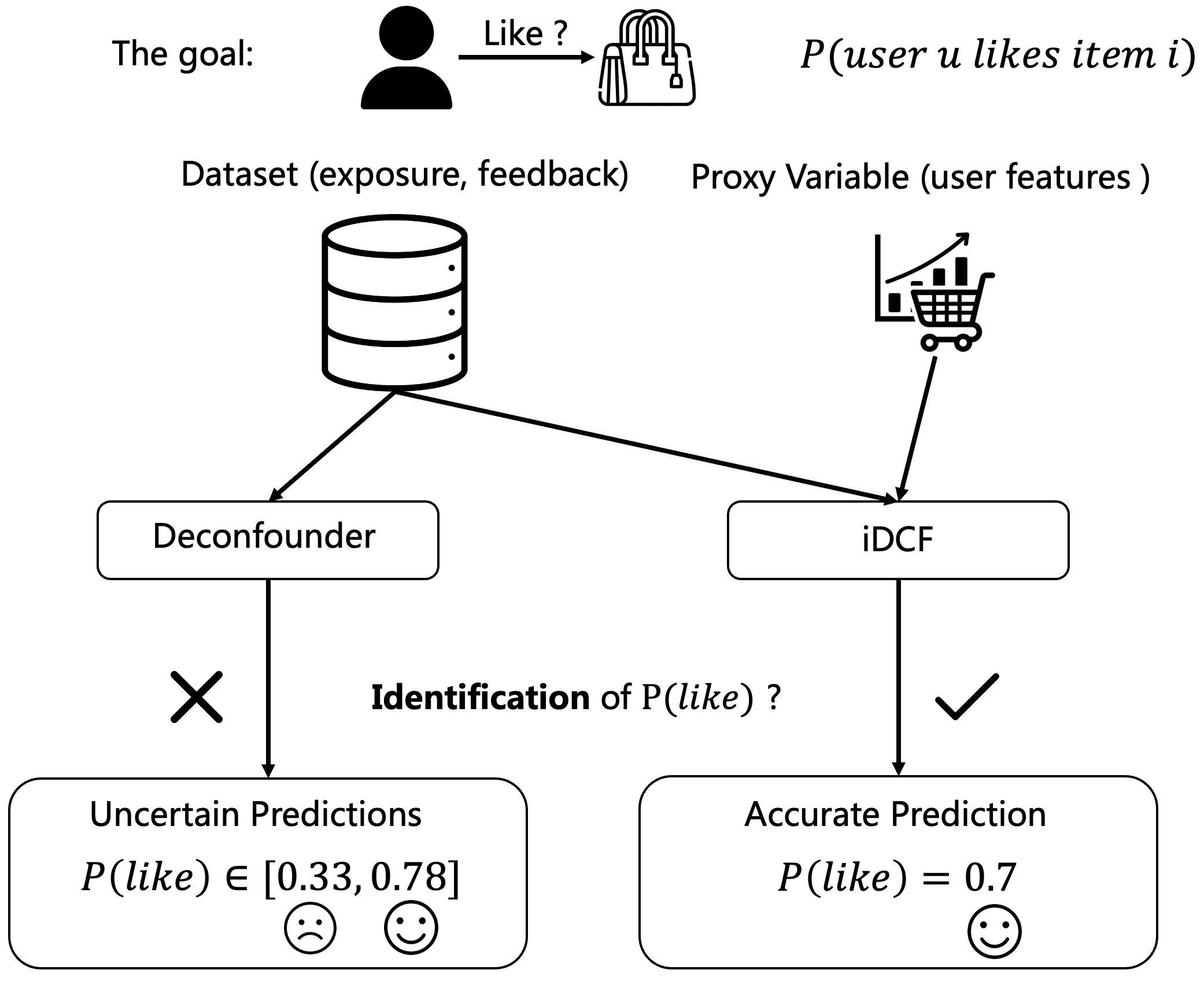
Figure 1. When predicting the user’s feedback, the non-identification of the user’s counterfactual feedback will make the recommendation method yield different feasible predictions (probabilities in the interval) that are compatible with the given dataset and will not converge, even with infinite data, leading to the uncertainty of the user’s feedback. See Example 3.1 for more details.

Hence, a glaring issue in the current practice in the recommender systems falls onto the identifiability of the user’s counterfactual feedback (potential outcome) in the presence of unmeasured confounders. This paper focuses on identifying the potential outcome by mitigating the unmeasured confounding bias.

As the user’s exposure history is helpful but not enough to infer the unmeasured confounder and identify the counterfactual feedback, additional information is required. Fortunately, such information can be potentially accessed through users’ features and historical interactions with the system. Using the previous example, while the user’s socio-economic status (unmeasured confounder) cannot be directly accessed, we can access the user’s consumption level from his recently purchased items, whose prices will be beneficial in inferring the user’s socio-economic status.

To this end, we formulate the debiasing recommendation problem as a causal inference problem with multiple treatments (different items to be recommended), and utilize the proximal causal inference technique (Tchetgen et al., 2020) which assumes the availability of a proxy variable (e.g., user’s consumption level), which is a descendant of the unmeasured confounder (e.g., user’s socio-economic status). Theoretically, the proxy variable can help infer the unmeasured confounder and the effects of exposure and confounders on the feedback. This leads to the identification of the potential outcome (see our Theorem 4.3), which is crucial for accurate predictions of users’ counterfactual feedback to items that have not been exposed. Practically, we choose user features as proxy variables since they are commonly found in recommender system datasets and the theoretical requirement of proxy variables is easier to be satisfied compared with the instrumental variables and mediators (Miao et al., 2022).

Specifically, we propose a novel approach to address unmeasured confounding bias in the task of debiasing recommender system, referred to as the identifiable deconfounder (iDCF). The proposed method is feedback-model-agnostic and can effectively handle situations where unmeasured confounders are present. iDCF utilizes the user’s historical interactions and additional observable proxy variables to infer the latent confounder effectively with identifiability. Then, the learned confounder is used to train the feedback prediction model that estimates the combined effect of confounders and exposure on the user’s feedback. In the inference stage, the adjustment method (Robins, 1986) is applied to mitigate confounding bias by taking the expectation over the learned confounder.

We evaluate the effectiveness of iDCF on a variety of datasets, including both real-world and synthetic, which demonstrate its encouraging performance and robustness regarding different confounding effects and data density in predicting user feedback. Moreover, on the synthetic dataset with the ground-truth of the unmeasured confounder known, we also explicitly show that iDCF can learn a better latent confounder in terms of identifiability.

Our main contributions are summarized as follows:

• We highlight the importance of identification of potential outcome distribution in the task of debiasing recommendation systems. Moreover, we demonstrate the non-identification issue of the Deconfounder method, which can lead to inaccurate feedback prediction due to confounding bias.

• We propose a general recommendation framework that utilizes proximal causal inference to address the non-identification issue in the task of debiasing recommendation systems and provides theoretical guarantees for mitigating the bias caused by unmeasured confounders.

• We conduct extensive experiments to show the superiority and robustness of our methods in the presence of unmeasured confounders.

2. Related work

2.1. Deconfounding in Recommendation

As causal inference becomes a popular approach in debiasing recommendation systems and examining relationships between variables (Robins, 1986; Pearl, 2009), researchers now focus more on the challenge of confounding bias. Confounding bias is prevalent in recommendation systems due to various confounding factors. For example, item popularity can create a popularity bias and be considered as a confounder. Several studies have addressed specific confounding biases, such as item popularity (Zhang et al., 2021; Wang et al., 2021; Wei et al., 2021), video duration (Zhan et al., 2022), video creator (He et al., 2022), and selection bias (Liu et al., 2022).

However, many unmeasured confounders may also exist, which make the classical deconfounding methods like inverse propensity weighting (IPW) not applicable. To deal with the confounding bias in the presence of unmeasured confounders, (Ding et al., 2022) assumes a bounded confounding effect on the exposure and applies robust optimization to improve the worst-case performance of recommendation models, (Zhu et al., 2022b; Xu et al., 2021; Si et al., 2022) take additional signals as mediators or instrumental variables to eliminate confounding bias. (Wang et al., 2022) assumes the existence of several environments to apply invariant learning. As shown in our later experiments, these additional strong assumptions on unmeasured confounders can lead to sub-optimal recommendation performance. Moreover, they also fail to provide a theoretical guarantee of the identification of users’ counterfactual feedback.

There is also another line of work (Wang et al., 2020; Zhu et al., 2022a) that considers the multiple-treatment settings (Wang and Blei, 2019) and infers substitute confounders from the user’s exposure to incorporate them into the preference prediction models. However, these methods cannot guarantee the identification of the user’s preference, which may lead to inconsistent, thus poor recommendation performance.

2.2. Proximal Causal Inference

Proximal causal inference (Kuroki and Pearl, 2014; Tchetgen et al., 2020; Miao et al., 2018a, b) assumes the existence of proxy variables of unmeasured confounders in the single-treatment regime, and the goal is to leverage proxy variables to identify causal effects. Kuroki and Pearl (Kuroki and Pearl, 2014) study the identification strategy in the different causal graphs. Miao et al. (Miao et al., 2018a) generalize their strategy and show nonparametric identification of the causal effect with two independent proxy variables. Miao et al. (Miao et al., 2018b) further use negative control exposure/outcome to explain the usages of proxy variables intuitively. However, these methods usually rely on informative proxy variables to infer the unmeasured confounders, while our method formulates the recommendation problem in the multiple treatment setting, which enables us to leverage information from the user’s exposure to infer the unmeasured confounder. This relaxes the requirement on the proxy variables and still theoretically guarantees the identification of the potential outcome (Miao et al., 2022).

3. Problem formulation

In this section, we first analyze the recommendation problem from a causal view in the presence of unmeasured confounders. Then we show that Deconfounder (Wang et al., 2020), one of the widely-used methods for recommendations with unobserved confounder, suffers the non-identification issue, i.e., it cannot predict the user’s preference consistently, through an illustrative example. This observation motivates our method, which we will detail in the next section.

3.1. Notations

We start with the notations used in this work. Let scalars and vectors be signified by lowercase letters (e.g., $a$) and boldface lowercase letters (e.g., $\boldsymbol{a}$), respectively. Subscripts signify element indexes. For example, $a_{i}$ is the $i$-th element of the vector $\boldsymbol{a}$. The superscript of a potential outcome denotes its corresponding treatment (e.g., $r_{ui}^{\boldsymbol{a}}$).

We adopt the potential outcome framework (Rubin, 1974) with multiple treatments (Wang and Blei, 2019) to formulate the problem. The causal graph is shown in Figure 2. Let $\mathcal{U}=\{u\}$ and $\mathcal{I}=\{i\}$ denote the set of users and items, respectively with $|\mathcal{U}|=m,|\mathcal{I}|=n$. We define the following components of the framework:

• Multiple treatments: $\boldsymbol{a}_{u}=[a_{u1},a_{u2},\dots,a_{un}]\in\{0,1\}^{n}$ is the observed exposure status of user $u$, where $a_{ui}=1$ ($a_{ui}=0$) means item $i$ was exposed to user $u$ (not exposed to user $u$) in history.

• Observed outcome: $r_{ui}$ denotes the observed feedback of the user-item pair $(u,i)$ and $\boldsymbol{r}_{u}=[r_{u1},...,r_{un}]$ signifies the observed feedbacks of user $u$.

• Potential outcome: $r_{ui}^{\boldsymbol{a}}$ denotes the potential outcome that would be observed if the user’s exposure had been set to the vector value $\boldsymbol{a}\in\{0,1\}^{n}$. Following previous work (Wang et al., 2020), we assume $r_{ui}^{\boldsymbol{a}}$ is only affected by the exposure of item $i$ to user $u$.

• Unmeasured confounder: $\boldsymbol{z}_{u}\in\mathbb{R}^{d}$ (e.g., the user’s socio-economic status) denotes the d-dimensional unmeasured confounder that causally influences both user’s exposures $\boldsymbol{a}_{u}$ and feedback $\boldsymbol{r}_{u}$.

Problem Statement. Given observational data $\{\boldsymbol{a}_{u},\boldsymbol{r}_{u}\}_{u\in\mathcal{U}}$, a recommendation algorithm aims to accurately predict the feedback of user $u$ on item $i$ if the item had been exposed to $u$, i.e., the expectation of the potential outcome $E[r_{ui}^{\boldsymbol{a}}]$, where $a_{i}=1$. Practically, for a user $u$, items are ranked by the predicted $E[r_{ui}^{\boldsymbol{a}}]$ such that the user will likely give positive feedback to items ranked in top positions.

However, in real-world scenarios, as the data of the recommendation system is naturally collected as users interact with the recommended items without randomized controlled trials, there usually exists some confounder, $\boldsymbol{z}_{u}$ as shown in Figure 2, which affects both the user $u$’s exposure status $\boldsymbol{a}_{u}$ (i.e., the treatment) and the user’s feedback on items $\boldsymbol{r}_{u}$ (i.e., the outcome), resulting in possible spurious correlations when the user’s feedback is simply estimated by $p(r_{ui}|\boldsymbol{a}_{u})$. For instance, the user’s socio-economic status can lead to confounding bias when predicting the user’s counterfactual feedback (See the example in Section 1).

Previous work (Wang et al., 2021; Zhang et al., 2021; Zhan et al., 2022; Mondal et al., 2022) takes $\boldsymbol{z}_{u}$ as a specific factor, for example, item popularity, video duration, video creators, etc. But under most real-world circumstances, we cannot access the complete information of $\boldsymbol{z}_{u}$. Thus, this work focuses on a more general problem setting where $\boldsymbol{z}_{u}$ is an unmeasured confounder. As shown in Figure 2, $\boldsymbol{z}_{u}$ is a latent variable represented by a shaded node.

(a) Without proxy variables

(b) With a proxy variable

Figure 2. Causal graphs with multiple treatments for recommendation systems. $\boldsymbol{a}_{ui}$: exposure of user $u$ to item $i$, $r_{ui}$: feedback of user $u$ on item $i$, $\boldsymbol{z}_{u}$: the unmeasured confounder, $\boldsymbol{w}_{u}$: a proxy variable of the confounder.

3.2. Identification with unmeasured confounder

To learn the counterfactual feedback from user $u$ on item $i$, i.e., $E[r_{ui}^{\boldsymbol{a}}]$, the identification of the potential outcome distribution $p(r_{ui}^{\boldsymbol{a}})$ from observational data is required. In general, accurately predicting a user’s feedback through data-driven models is only possible when causal identifiability has been established.

When all confounders are measured, $p(r_{ui}^{\boldsymbol{a}})$ can be identified through the classical g-formula (Robins, 1986) as follows:

(1) $$p(r_{ui}^{\boldsymbol{a}})=E_{\boldsymbol{z}_{u}}[p(r_{ui}|\boldsymbol{a},\boldsymbol{z}_{u})].$$

When an unmeasured confounder exists, as shown in Figure 2, it becomes much more challenging to identify $p(r_{ui}^{\boldsymbol{a}})$ as the g-formula is no longer applicable. Previously, Wang et al. (Wang et al., 2020) assumed the unmeasured confounder $\boldsymbol{z}_{u}$ is a common cause of each exposure $a_{ui}$ and proposed Deconfounder to learn $p(r_{ui}^{\boldsymbol{a}})$ with unmeasured confounders. Deconfounder first learns a substitute confounder $\hat{\boldsymbol{z}}_{u}$ from the exposure vector $\boldsymbol{a}_{u}$ to approximate the true confounder $\boldsymbol{z}_{u}$, and directly applies the g-formula in Eq. 1 to learn $p(r_{ui}^{\boldsymbol{a}})$.

Non-Identification of Deconfounder. While the high-level idea is promising, Deconfounder fails to guarantee the identification of $p(r_{ui}^{\boldsymbol{a}})$ (D’Amour, 2019; Grimmer et al., 2020). As shown by the following example, even in a relatively optimistic case where the substitute confounder $\hat{z}_{u}$ can be uniquely determined from the exposure vector $\boldsymbol{a}_{u}$, Deconfounder cannot identify $p(r_{ui}^{\boldsymbol{a}})$. In other words, $p(r_{ui}^{\boldsymbol{a}})$ takes different values under different circumstances, leading to the inconsistent prediction of the user’s feedback.

Example 3.1 (Failure of Deconfounder (Wang et al., 2020) in identification.).

Consider a recommendation scenario following the causal graph in Figure 2, with the confounder $z_{u}$, the exposure status $a_{ui}$, and the feedback $r_{ui}$ assumed to be binary random variables.

We assume $n\geq 3$ to ensure a unique factorization of $p(\boldsymbol{a}_{u})$ (Kruskal, 1989), such that the inferred substitute confounder $\hat{z}_{u}$ in Deconfounder can be uniquely identified from exposure vector $\boldsymbol{a}$. In other words, $p(\hat{z}_{u}=1)$ and $p(\hat{z}_{u}=1|\boldsymbol{a})$ are known. Besides, $p(r_{ui}=1|\boldsymbol{a})$, the probability that user $u$ will give positive feedback to the item $i$ condition on exposure vector $\boldsymbol{a}$, can also be inferred given a dataset.

Recall that Deconfounder learns $p(r_{ui}^{\boldsymbol{a}})$ by applying the g-formula in Eq. 1 with the inferred substitute confounder $\hat{z}_{u}$ as follows:

(2) $$\begin{array}[]{lcl}p(r_{ui}^{\boldsymbol{a}}=1)&=&\sum_{z\in\{0,1\}}p(\hat{z}_{u}=z)p(r_{ui}^{\boldsymbol{a}}=1|\boldsymbol{a},\hat{z}_{u}=z)\\ &=&\sum_{z\in\{0,1\}}p(\hat{z}_{u}=z)\frac{p(r_{ui}^{\boldsymbol{a}}=1,\hat{z}_{u}=z|\boldsymbol{a})}{p(\hat{z}_{u}=z|\boldsymbol{a})}.\\ \end{array}$$

For ease of illustration, we denote $p_{01|\boldsymbol{a}}:=p(\hat{z}_{u}=0,r_{ui}=1|\boldsymbol{a}),\pi_{\hat{z}_{u}=1}:=p(\hat{z}_{u}=1),\pi_{\hat{z}_{u}=1|\boldsymbol{a}}:=p(\hat{z}_{u}=1|\boldsymbol{a}),\pi_{r_{ui}=1|\boldsymbol{a}}:=p(r_{ui}=1|\boldsymbol{a})$ in the rest of the paper, then we get:

(3) $$p(r_{ui}^{\boldsymbol{a}}=1)=(1-\pi_{\hat{z}_{u}=1})\frac{p_{01|\boldsymbol{a}}}{1-\pi_{\hat{z}_{u}=1|\boldsymbol{a}}}+\pi_{\hat{z}_{u}=1}\frac{p_{11|\boldsymbol{a}}}{\pi_{\hat{z}_{u}=1|\boldsymbol{a}}}$$

As we assumed before, $\pi_{\hat{z}_{u}=1}$ and $\pi_{\hat{z}_{u}=1|\boldsymbol{a}}$ are known, thus it remains to identify $p_{01|a}$, and $p_{11|a}$ to calculate $p(r_{ui}^{\boldsymbol{a}}=1)$. However, $p_{01|a}$ and $p_{11|a}$ can not be uniquely determined since there are four unknown entries $\{p_{zr|a},z,r\in\{0,1\}\}$ with three constraints:

(4) $$\sum_{z}\sum_{r}p_{zr|a}=1,\sum_{r}p_{1r|a}=\pi_{\hat{z}_{u}=1|a},\sum_{z}p_{z1}=\pi_{r_{ui}=1|a},$$

where the first constraint is the normalization of joint probabilities, and the next two are marginal constraints. For example, the second constraint is due to

(5) $$p(\hat{z}_{u}=1,r_{ui}=0|\boldsymbol{a})+p(\hat{z}_{u}=1,r_{ui}=1|\boldsymbol{a})=p(\hat{z}_{u}=1|\boldsymbol{a}).$$

When $\pi_{\hat{z}_{u}=1|\boldsymbol{a}}$ is not degenerated, i.e.,$\pi_{\hat{z}_{u}=1|\boldsymbol{a}}\neq 1$ or $0$, which holds in the recommendation scenario, the four unknown entries cannot be uniquely determined because there remains one degree of freedom (Strang et al., 1993). For example, if we take $p_{11|a}$ as the free variable, then it can be any value in the following feasible range:

$$\max\{0,\pi_{\hat{z}_{u}=1|\boldsymbol{a}}+\pi_{r_{ui}=1|\boldsymbol{a}}-1\}\leq p_{11|a}\leq\min\{\pi_{\hat{z}_{u}=1|\boldsymbol{a}},\pi_{r_{ui}=1|\boldsymbol{a}}\},$$

implying $p(r_{ui}^{\boldsymbol{a}}=1)$ calculated as in Eq. 3 will also be in a range. In other words, $p(r_{ui}^{\boldsymbol{a}}=1)$ cannot be identified.

To make it more explicit, consider this concrete example. Assuming $\pi_{\hat{z}_{u}=1}=0.5,\pi_{\hat{z}_{u}=1|\boldsymbol{a}}=0.2,\pi_{r_{ui}=1|\boldsymbol{a}}=0.6$, then $p_{11|\boldsymbol{a}}$ can be any value in $[0,0.1]$, leading to the feasible range of $p(r_{ui}^{\boldsymbol{a}})\in[0.33,0.78]$. When the commonly used prediction threshold of $0.5$ is applied, one will get an inconsistent prediction of the user $u$’s preference over item $i$, since $p(r_{ui}^{\boldsymbol{a}}=1)=0.78$ implies user $u$ will prefer the item $i$, while $p(r_{ui}^{\boldsymbol{a}}=1)=0.33$ not. Obviously, the distortion will be even larger when directly ranking items according to $p(r_{ui}^{\boldsymbol{a}}=1)$ when its identification cannot be guaranteed.

4. Method

In this section, we show how proximal causal inference (Tchetgen et al., 2020) can help ensure the identification of user’s counterfactual feedback $p(r_{ui}^{\boldsymbol{a}})$. We start by showing that with a proxy variable (e.g., user features), one can identify $p(r_{ui}^{\boldsymbol{a}})$ in Example 3.1. We then propose a feedback-model-agnostic framework iDCF, for the identification of user’s counterfactual feedback with unmeasured confounders in general recommendation scenarios with a theoretical guarantee.

4.1. Framework

A natural question following Example 3.1 is: How to fix the identification issue of $p(r_{ui}^{\boldsymbol{a}})$ so as to predict users’ counterfactual feedback uniquely and accurately? Intuitively, if more information about the unmeasured confounder can be provided, i.e., more constraints in Eq. 4, $p(r_{ui}^{\boldsymbol{a}})$ can be uniquely determined, which motivates the usage of proximal causal inference (Tchetgen et al., 2020).

Inspired by the above intuition, we reformulate the recommendation problem with the unmeasured confounder from the view of proximal causal inference. Specifically, we assume that one can observe additional information of user $u$, called proxy variable $w_{u}$, which is directly affected by the unmeasured confounder $\boldsymbol{z}_{u}$ and independent of the feedback $r_{ui}$ given the unmeasured confounder $\boldsymbol{z}_{u}$ and the exposure vector $\boldsymbol{a}_{u}$, i.e.,:

$$\boldsymbol{w}_{u}=g(\boldsymbol{z}_{u}),\boldsymbol{w}_{u}\perp r_{ui}|(\boldsymbol{z}_{u},\boldsymbol{a}_{u}),$$

where $g$ is an unknown function. Fortunately, in the recommendation scenario, such a proxy variable can be potentially accessed through the user’s features, including user profiles summarized from interaction history. For example, when the unmeasured confounder $\boldsymbol{z}_{u}$ is the user’s socio-economic status, which usually cannot be directly accessed, possibly due to privacy concerns, one can take the proxy variable as the average price of items that the user recently purchased, which is pretty helpful in inferring the user’s socio-economic status since high consumption often implies high socio-economic status. Moreover, such a proxy variable will not directly affect the user’s feedback if the user’s socio-economic status is already given.

We first show that the user’s counterfactual feedback $p(r_{ui}^{\boldsymbol{a}})$ in Example 3.1 can be identified with a proxy variable $\boldsymbol{w}_{u}$.

Example 4.1 (Success in identifying $p(r_{ui}^{\boldsymbol{a}})$ with proxy variable).

Following the settings in Example 3.1, we introduce an observable proxy variable $w_{u}$ that indicates the user’s consumption level affected by the socio-economics status $z_{u}$ in the recommendation platform, the corresponding causal graph is shown in Figure 2(b). We assume $w_{u}$ is a Bernoulli random variable with mean $\mu(\boldsymbol{z}_{u})\in(0,1)$ and $w_{u}$ is correlated with $z_{u}$ condition on $\boldsymbol{a}_{u}$.

Similar to Example 3.1, $p(r_{ui}=1|\boldsymbol{a},w_{u})$, the probability that user $u$ will give positive feedback to item $i$ with given exposure status $\boldsymbol{a}$ and consumption level $w_{u}$, can be inferred from the given dataset, and $p(\hat{z}_{u}|\boldsymbol{a},w_{u})$ is assumed to be uniquely determined by factor models. Again, for the ease of illustration, we denote $\pi_{r_{ui}=1|\boldsymbol{a},w}:=p(r_{ui}=1|\boldsymbol{a}_{u}=\boldsymbol{a},w_{u}=w)$ and $\pi_{\hat{z}_{u}=1|\boldsymbol{a},w}:=p(\hat{z}_{u}=1|\boldsymbol{a}_{u}=\boldsymbol{a},w_{u}=w)$. Now, while there are still four unknown entries $\{p_{zr|a},z,r\in\{0,1\}\}$ as in Eq. 4, the number of constraints increases from three to four with the two conditional marginal distributions $\pi_{r_{ui}=1|\boldsymbol{a},w=0}$ and $\pi_{r_{ui}|\boldsymbol{a},w=1}$, i.e.,

(6) $$\begin{array}[]{ll}\sum_{z}\sum_{r}p_{zr|\boldsymbol{a}}=1,&\sum_{z}p_{z1|\boldsymbol{a}}\frac{\pi_{\hat{z}_{u}=z|\boldsymbol{a},w=1}}{\pi_{\hat{z}_{u}=z|\boldsymbol{a}}}=\pi_{r_{ui}=1|\boldsymbol{a},w=1},\\ \sum_{r}p_{1r|\boldsymbol{a}}=\pi_{\hat{z}_{u}=1|\boldsymbol{a}},&\sum_{z}p_{z1|a}\frac{\pi_{\hat{z}_{u}=z|\boldsymbol{a},w=0}}{\pi_{\hat{z}_{u}=z|\boldsymbol{a}}}=\pi_{r_{ui}=1|\boldsymbol{a},w=0}.\end{array}$$

The following lemma shows the identification result of $p(r_{ui}^{\boldsymbol{a}})$.

Lemma 4.2.

There exists a unique solution of $\{p_{zr|a},z,r\in\{0,1\}\}$ from Eq. 6, leading to the identification of the potential outcome $p(r_{ui}^{\boldsymbol{a}})$ calculated from Eq. 2.

General framework of identifying the user’s counterfactual feedback $p(r_{ui}^{\boldsymbol{a}})$ with proxy variables. Next, we show how to identify $p(r_{ui}^{\boldsymbol{a}})$ with proxy variables in general. Observing that

(7) $$\begin{split}p(r_{ui}^{\boldsymbol{a}})&=E_{\hat{\boldsymbol{z}}_{u}}[p(r_{ui}|\boldsymbol{a},\hat{\boldsymbol{z}}_{u})]=\int_{\boldsymbol{z}}p(\hat{\boldsymbol{z}}_{u}=\boldsymbol{z})p(r_{ui}|\boldsymbol{a},\hat{\boldsymbol{z}}_{u}=\boldsymbol{z})d\boldsymbol{z},\end{split}$$

the key is to infer $p(\hat{\boldsymbol{z}}_{u})$ and $p(r_{ui}|\boldsymbol{a},\hat{\boldsymbol{z}}_{u})$, yielding the following two-step procedure of the proposed method iDCF:

• Learning Latent Confounder: This stage aims to learn a latent confounder $\hat{\boldsymbol{z}}_{u}$ with the help of proxy variables, such that the learned $\hat{\boldsymbol{z}}_{u}$ is equivalent to the true unmeasured confounder $\boldsymbol{z}_{u}$ up to some transformations (Khemakhem et al., 2020; Miao et al., 2022) and can provide additional constraints to infer the user’s feedback $r_{ui}$, which cannot be achieved by the substitute confounder in Deconfounder. Specifically, we aim to learn its prior distribution, i.e., $p(\hat{z}_{u})$. Since

  (8) $$p(\hat{\boldsymbol{z}}_{u}=z)=E_{\boldsymbol{a}_{u},\boldsymbol{w}_{u}}[p(\hat{\boldsymbol{z}}_{u}|\boldsymbol{a}_{u},\boldsymbol{w}_{u})],$$

  and $p(\boldsymbol{a}_{u},\boldsymbol{w}_{u})$ is measured from the dataset, thus the main challenge is to learn $p(\hat{z}_{u}|\boldsymbol{a}_{u},\boldsymbol{w}_{u})$, which can be learned by reconstructing the exposure vector $\boldsymbol{a}_{u}$ based solely on $\boldsymbol{w}_{u}$, since:

  (9) $$p(\boldsymbol{a}_{u}|\boldsymbol{w}_{u})=\int_{\boldsymbol{z}}p(\boldsymbol{a}_{u}|\hat{\boldsymbol{z}}_{u}=\boldsymbol{z})p(\hat{\boldsymbol{z}}_{u}=\boldsymbol{z}|\boldsymbol{a}_{u},\boldsymbol{w}_{u})d\boldsymbol{z}.$$

  For example, we can apply the widely-used iVAE (Khemakhem et al., 2020) model, then $p(\hat{\boldsymbol{z}}_{u}|\boldsymbol{a}_{u},\boldsymbol{w}_{u})$ and $p(\boldsymbol{a}_{u}|\hat{\boldsymbol{z}}_{u})$ are estimated by the encoder and the decoder respectively.

• Feedback with given latent confounder: This stage aims to learn $p(r_{ui}|\boldsymbol{a}_{u},\hat{\boldsymbol{z}}_{u})$, i.e., user $u$’s feedback on item $i$ under the fixed exposure vector $\boldsymbol{a}_{u}$ and latent confounder $\hat{\boldsymbol{z}}_{u}$. With the help of $p(\hat{\boldsymbol{z}}_{u}|\boldsymbol{a}_{u},\boldsymbol{w}_{u})$ learned in the first stage, one can infer it by directly fitting the observed users’ feedback $p(r_{ui}|\boldsymbol{a}_{u},\boldsymbol{w}_{u})$, since:

  (10) $$p(r_{ui}|\boldsymbol{a}_{u},\boldsymbol{w}_{u})=\int_{z}p(r_{ui}|\hat{z}_{u}=z,\boldsymbol{a}_{u})p(\hat{z}_{u}=z|\boldsymbol{a}_{u},\boldsymbol{w}_{u})dz.$$

Then the potential outcome (i.e., the user’s counterfactual feedback) distribution $p(r_{ui}^{\boldsymbol{a}})$ is identified by applying Eq. 7. The following theorem shows the general theoretical guarantee on identification of $p(r_{ui}^{\boldsymbol{a}})$ through the aforementioned two-step procedure.

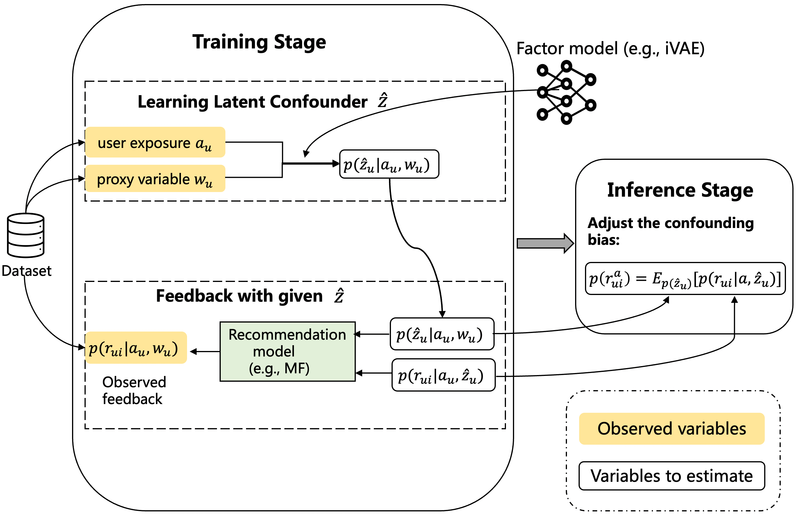
Figure 3. The framework of the proposed method iDCF.

Theorem 4.3 (Identification with proxy variable (Miao et al., 2022)).

Under the consistency, ignorability, positivity, exclusion restriction, equivalence, and completeness assumptions, for any latent joint distribution $p(\boldsymbol{a}_{u},\hat{\boldsymbol{z}}_{u}|\boldsymbol{w}_{u})$ that solves $p(\boldsymbol{a}_{u}|\boldsymbol{w}_{u})=\int_{\boldsymbol{z}}p(\boldsymbol{a}_{u},\hat{\boldsymbol{z}}_{u}=\boldsymbol{z}|\boldsymbol{w}_{u})d\boldsymbol{z}$, there exists a unique solution $p(r_{ui}|\hat{\boldsymbol{z}}_{u},\boldsymbol{a}_{u})$ to the equation Eq. 10 and the potential outcome distribution is identified by Eq. 7.

Remark 1 (About assumptions).

Note that Theorem 4.3 relies on several assumptions: consistency, ignorability, positivity, exclusion restriction, equivalence, and completeness. The first 3 assumptions are standard assumptions in causal inference (Wang et al., 2021; Zhan et al., 2022). Informally, exclusion restriction requires the proxy variable to be independent of the user’s feedback conditioned on the confounder and exposure, which can be reasonable in a recommendation system since the proxy variable (e.g., user’s consumption level) is mainly used to implicitly infer the hidden confounder (e.g., user’s income) that directly affects user’s feedback. Equivalence requires the unmeasured confounder can be identified from the dataset up to a one-to-one transformation, which is also feasible with various factor models (Khemakhem et al., 2020; Kruskal, 1989). Completeness requires that the proxy variable contains enough information to guarantee the uniqueness of the statistic about the hidden confounder, which can also be feasible in recommendation scenarios since the variability in the unmeasured confounders (e.g., user’s socio-economics status) is usually captured by variability in the user features (e.g., user’s consumption level).

4.2. Practical Implementation

Next, we describe how the proposed iDCF implements the identification steps described in Section 4.1 practically. We need to specify:

• Training Stage: (1) How to learn the latent confounder, i.e., $p(\hat{\boldsymbol{z}}_{u})$ in Eq. 8? As discussed in Section 4.1, the main challenge is to learn $p(\hat{z}_{u}|\boldsymbol{a}_{u},\boldsymbol{w}_{u})$. (2) How does our method learn users’ feedback with the given latent confounder, i.e., $p(r_{ui}|\boldsymbol{a}_{u},\hat{\boldsymbol{z}}_{u})$?

• Inference Stage. With $p(\hat{\boldsymbol{z}}_{u})$ and $p(r_{ui}|\boldsymbol{a}_{u},\hat{\boldsymbol{z}}_{u})$ learned in the training stage, how does the proposed iDCF framework infer the unbiased feedback of users following Eq. 7?

Learning Latent Confounder. We use iVAE (Khemakhem et al., 2020) to learn the latent confounder, since it is widely used to identify latent variables up to an equivalence relation (see the Definition 2 in (Khemakhem et al., 2020)) by leveraging auxiliary variables which are equivalent to proxies. Specifically, we simultaneously learn the deep generative model and approximate posterior $q_{\phi}(\hat{\boldsymbol{z}}_{u}|\boldsymbol{a}_{u},\boldsymbol{w}_{u})$ of the true posterior $p_{\theta}(\hat{\boldsymbol{z}}_{u}|\boldsymbol{a}_{u},\boldsymbol{w}_{u})$ by maximizing $\mathcal{L}(\theta,\phi)$, which is the evidence lower bound (ELBO) of the likelihood $\log p_{\theta}(\boldsymbol{a}_{u}|\boldsymbol{w}_{u})$:

(11) $$\begin{split}&E[\log p_{\theta}(\boldsymbol{a}_{u}|\boldsymbol{w}_{u})]\geq\mathcal{L}(\theta,\phi):=\\ =&E[\underbrace{E_{q_{\phi}(\hat{\boldsymbol{z}}_{u}|\boldsymbol{a}_{u},\boldsymbol{w}_{u})}[\log p_{\theta}(\hat{\boldsymbol{z}}_{u}|\boldsymbol{w}_{u})-\log q_{\phi}(\hat{\boldsymbol{z}}_{u}|\boldsymbol{a}_{u},\boldsymbol{w}_{u})]}_{I}\\ &+\underbrace{E_{q_{\phi}(\hat{\boldsymbol{z}}_{u}|\boldsymbol{a}_{u},\boldsymbol{w}_{u})}[\log p_{\theta}(\boldsymbol{a}_{u}|\hat{\boldsymbol{z}}_{u})]}_{II}].\end{split}$$

where according to the causal graph in Figure 2(b), $\log p_{\theta}(\boldsymbol{a}_{u},\hat{\boldsymbol{z}}_{u}|\boldsymbol{w}_{u})$ is further decomposed as follows:

(12) $$\begin{split}\log p_{\theta}(\boldsymbol{a}_{u},\hat{\boldsymbol{z}}_{u}|\boldsymbol{w}_{u})=&\log p_{\theta}(\boldsymbol{a}_{u}|\hat{\boldsymbol{z}}_{u},\boldsymbol{w}_{u})+\log p_{\theta}(\hat{\boldsymbol{z}}_{u}|\boldsymbol{w}_{u})\\ =&\log p_{\theta}(\boldsymbol{a}_{u}|\hat{\boldsymbol{z}}_{u})+\log p_{\theta}(\hat{\boldsymbol{z}}_{u}|\boldsymbol{w}_{u}).\end{split}$$

Following (Khemakhem et al., 2020), we choose the prior $p_{\theta}(\hat{\boldsymbol{z}}_{u}|\boldsymbol{w}_{u})$ to be a Gaussian location-scale family, and use the reparameterization trick (Kingma and Welling, 2013) to sample $\hat{z}_{u}$ from the approximate posterior $q_{\phi}(\hat{\boldsymbol{z}}_{u}|\boldsymbol{a}_{u},\boldsymbol{w}_{u})$ as

(13) $$\begin{split}p_{\theta}(\hat{\boldsymbol{z}}_{u}|\boldsymbol{w}_{u})&:=N(\mu_{w}(\boldsymbol{w}_{u}),v_{w}(\boldsymbol{w}_{u})),\\ q_{\phi}(\hat{\boldsymbol{z}}_{u}|\boldsymbol{a}_{u},\boldsymbol{w}_{u})&:=N(\mu_{aw}(\boldsymbol{a}_{u},\boldsymbol{w}_{u}),v_{aw}(\boldsymbol{a}_{u},\boldsymbol{w}_{u})),\end{split}$$

where $\mu_{w},v_{w},\mu_{aw},v_{aw}$ are modeled by $4$ different MLP models. To this end, the calculation of the expectation $I$ of Eq. (11) can be converted to the calculation of the Kullback-Leibler divergence of two Gaussian distributions:

$$\begin{split}&E_{q_{\phi}(\hat{\boldsymbol{z}}_{u}|\boldsymbol{a}_{u},\boldsymbol{w}_{u})}[\log p_{\theta}(\hat{\boldsymbol{z}}_{u}|\boldsymbol{w}_{u})-\log q_{\phi}(\hat{\boldsymbol{z}}_{u}|\boldsymbol{a}_{u},\boldsymbol{w}_{u})]\\ =&-KL(N(\mu_{aw}(\boldsymbol{a}_{u},\boldsymbol{w}_{u}),v_{aw}(\boldsymbol{a}_{u},\boldsymbol{w}_{u}),N(\mu_{w}(\boldsymbol{w}_{u}),v_{w}(\boldsymbol{w}_{u}))).\end{split}$$

As for $II$, since the hidden confounder directly affects each element of the exposure vector, we use a factorized logistic model as $p_{\lambda}(\boldsymbol{a}_{u}|\boldsymbol{z}_{u})$, i.e., $p_{\lambda}(\boldsymbol{a}_{u}|\boldsymbol{z}_{u})=\prod_{i=1}^{n}Bernoulli(\boldsymbol{a}_{ui}|\boldsymbol{z}_{u})$, which is also modeled by a MLP $\mu_{z}(\boldsymbol{z})$. Then the log-likelihood $\log p_{\theta}(\boldsymbol{a}_{u}|\hat{\boldsymbol{z}}_{u})$ becomes the negative binary cross entropy:

$$\log p_{\theta}(\boldsymbol{a}_{u}|\hat{\boldsymbol{z}}_{u})=\sum_{i=1}^{n}\boldsymbol{a}_{ui}\log(\mu_{z}(\boldsymbol{z}_{u})_{i})+(1-\boldsymbol{a}_{ui})\log(1-\mu_{z}(\boldsymbol{z}_{u})_{i}).$$

Then, through maximizing Eq. 11, we are able to obtain the approximate posterior of latent confounder $q_{\phi}(\hat{\boldsymbol{z}}_{u}|\boldsymbol{a}_{u},\boldsymbol{w}_{u})$.

Feedback with given latent confounder. As shown in Eq. 9, with $q_{\phi}(\hat{\boldsymbol{z}}_{u}|\boldsymbol{a}_{u},\boldsymbol{w}_{u})$ estimated through iVAE, the user’s feedback on item $i$ with the latent confounder $\hat{\boldsymbol{z}}_{u}$, i.e., $p(r_{ui}|\boldsymbol{a}_{u},\hat{\boldsymbol{z}}_{u})$, can be learned by fitting a recommendation model on the observed users’ feedback. Following the assumption in Section 3.1 where $r_{ui}^{\boldsymbol{a}}$ is only affected by the exposure of item $i$ to user $u$, we use a point-wise recommendation model $f(u,i,\boldsymbol{z}_{u};\eta)$ parameterized by $\eta$ to estimate $p(r_{ui}|\boldsymbol{a}_{u},\hat{\boldsymbol{z}}_{u})$. Specifically, we adopt a simple additive model $f(u,i,\hat{\boldsymbol{z}}_{u};\eta)=f_{1}(u,i)+f_{2}(\hat{\boldsymbol{z}}_{u},i)$ that models the user’s intrinsic preference and the effect of the latent confounder separately. The corresponding loss function is:

(14) $$\mathcal{L}_{iDCF}(\eta)=\frac{1}{|\mathcal{D}|}\sum_{(u,i)\in\mathcal{D}}l(E_{q_{\phi}(\hat{\boldsymbol{z}}_{u}|\boldsymbol{a}_{u},\boldsymbol{w}_{u})}[f(u,i,\hat{\boldsymbol{z}}_{u};\eta)],r_{ui}),$$

where $l(\cdot,\cdot)$ is one of the commonly-used loss functions for recommendation systems, e.g., MSE loss and BCE loss.

Inference Stage. In practice, for most real-world recommendation datasets, the user’s feature $\boldsymbol{w}_{u}$ is invariant in the training set and test set. Therefore, identifying $p(r_{ui}^{\boldsymbol{a}})$ is equivalent to identifying $p(r_{ui}^{\boldsymbol{a}}|\boldsymbol{w}_{u})$ since $p(r_{ui}^{\boldsymbol{a}})=\int_{w}p(r_{ui}^{\boldsymbol{a}}|\boldsymbol{w}_{u}=w)p(\boldsymbol{w}_{u}=w)dw$ and $p(\boldsymbol{w}_{u}=w)=1$ for those specific $w$ associated with user $u$. The corresponding identification formula becomes:

(15) $$\begin{split}p(r_{ui}^{\boldsymbol{a}}|\boldsymbol{w}_{u})&=\int_{\boldsymbol{z}}p(\hat{\boldsymbol{z}}_{u}=\boldsymbol{z}|\boldsymbol{w}_{u})p(r_{ui}|\boldsymbol{a},\hat{\boldsymbol{z}}_{u}=\boldsymbol{z})d\boldsymbol{z}\\ &=E_{\hat{\boldsymbol{z}}_{u}|\boldsymbol{w}_{u}}[p(r_{ui}|\boldsymbol{a},\hat{\boldsymbol{z}}_{u})],\end{split}$$

where $p(r_{ui}|\boldsymbol{a},\hat{\boldsymbol{z}}_{u}=\boldsymbol{z})$ is estimated by the learned recommendation model $f(u,i,\boldsymbol{z}_{u};\eta)$ and $p(\hat{\boldsymbol{z}}_{u}=\boldsymbol{z}|\boldsymbol{w}_{u})$ is approximated by the encoder $q_{\phi}(\hat{\boldsymbol{z}}_{u}|\boldsymbol{a}_{u},\boldsymbol{w}_{u})$.

In summary, we first apply iVAE to learn the posterior distribution of the latent confounder $p(\hat{z}_{u}|\boldsymbol{a}_{u},\boldsymbol{w}_{u})$ for each user $u$, then leverage it to learn the user’s feedback estimator $f(u,i,\boldsymbol{z}_{u};\eta)$ in the training phase. Finally, we apply Eq. 15 to predict the deconfounded feedback in the inference phase. The pseudo-code of iDCF is shown in Algorithm 1.

5. Experiments

In this section, we conduct experiments to answer the following research questions:

• RQ1 Does the proposed iDCF outperform existing deconfounding methods for debiasing recommendation systems?

• RQ2 What is the performance of iDCF under different confounding effects and dense ratios of the exposure matrix?

• RQ3 How does the identification of latent confounders impact the performance of iDCF?

5.1. Experiment Settings

Dataset. Following previous work (Ding et al., 2022; Wang et al., 2020, 2022), we perform experiments on three real-world datasets: Coat , Yahoo!R3 and KuaiRand collected from different recommendation scenarios. Each dataset consists of a biased dataset of normal user interactions, and an unbiased uniform dataset collected by a randomized trial such that users will interact with randomly selected items. We use all biased data as the training set, 30% of the unbiased data as the validation set, and the remaining unbiased data as the test set. For Coat and Yahoo!R3, the feedback from a user to an item is a rating ranging from 1 to 5 stars. We take the ratings $\geq 4$ as positive feedback, and others as negative feedback. For KuaiRand, the positive samples are defined according to the signal ”IsClick” provided by the platform.

Moreover, to answer RQ2 and RQ3, we also generate a synthetic dataset with groundtruth of the unmeasured confounder known for in-depth analysis of the iDCF .

Table 1. The statistic of Coat, Yahoo!R3, and KuaiRand.

Dataset	#User	#Item	#Biased Data	#Unbiased Data
Coat	290	300	6,960	4,640
Yahoo! R3	5,400	1,000	129,179	54,000
KuaiRand	23,533	6,712	1,413,574	954,814

Baselines. We compare our method with the corresponding base models and the state-of-the-art deconfounding methods that can alleviate the confounding bias in recommendation systems in the presence of unmeasured confounders.

• MF (Koren et al., 2009) & MF with feature (MF-WF). We use the classical Matrix Factorization (MF) as the base recommendation model. Since our method utilizes user features, for a fair comparison, we consider MF-WF, a variant of MF model augmented with user features.

• DCF (Wang et al., 2020). Deconfounder (DCF) addresses the unmeasured confounder by learning a substitute confounder to approximate the true unmeasured confounder and applying the g-formula for debiasing. However, as discussed before, it fails to guarantee the identification of users’ feedback, leading to the inconsistent prediction of users’ feedback.

• IPS (Schnabel et al., 2016) & RD-IPS (Ding et al., 2022). IPS is a classical propensity-based deconfounding method that ignores the unmeasured confounder and directly leverages the exposure to estimate propensity scores to reweight the loss function. RD-IPS is a recent IPS-based deconfounding method that assumes the bounded confounding effect of the unmeasured confounders to derive bounds of propensity scores and applies robust optimization for robust debiasing. The implementation of the two methods leverages a small proportion of unbiased data to get more accurate propensity scores.

• InvPref (Wang et al., 2022). InvPref assumes the existence of multiple environments as proxies of unmeasured confounders and applies invariant learning (Bühlmann, 2020; Arjovsky et al., 2019) to learn the user’s invariant preference.

• DeepDCF-MF. DeepDCF (Zhu et al., 2022a) extends DCF by applying deep models and integrating the user’s feature into the feedback prediction model to control the variance of the model. For a fair comparison, we adapt their model with MF as the backbone model.

• iDCF-W. iDCF-W is a variant of iDCF that does not leverage proxy variables. We adopt VAE (Kingma and Welling, 2013) to learn the substitute confounder in such a scenario, with other parts staying the same with iDCF.

Implementation details. Due to space limitations, please refer to Appendix B.

5.2. Performance Comparison (RQ1)

The experimental results on the three real-world datasets are shown in Table 2. We can observe that:

Table 2. Recommendation performances on Coat, Yahoo!R3 and KuaiRand. The p-value under t-test between iDCF and the best baseline on each dataset is also provided.

Datasets	Coat		Yahoo!R3		KuaiRand
	NDCG@5	RECALL@5	NDCG@5	RECALL@5	NDCG@5	RECALL@5
MF	$0.5524\pm 0.0144$	$0.5294\pm 0.0227$	$0.5629\pm 0.0100$	$0.7129\pm 0.0106$	$0.3748\pm 0.0018$	$0.3247\pm 0.0013$
MF-WF	$\underline{0.5529}\pm 0.0101$	$\underline{0.5341}\pm 0.0143$	$0.5649\pm 0.0073$	$0.7144\pm 0.0086$	$0.3762\pm 0.0014$	$0.3255\pm 0.0013$
IPS	$0.5450\pm 0.0161$	$0.5260\pm 0.0191$	$0.5490\pm 0.0058$	$0.6967\pm 0.0096$	$0.3696\pm 0.0011$	$0.3224\pm 0.0009$
RD-IPS	$0.5448\pm 0.0147$	$0.5240\pm 0.0157$	$0.5550\pm 0.0051$	$0.7020\pm 0.0068$	$0.3690\pm 0.0016$	$0.3207\pm 0.0011$
InvPref	$0.5405\pm 0.0135$	$0.5295\pm 0.0225$	$0.5928\pm 0.0038$	$0.7414\pm 0.0052$	$0.3778\pm 0.0020$	$0.3283\pm 0.0014$
DCF	$0.5509\pm 0.0093$	$0.5329\pm 0.0152$	$0.5675\pm 0.0047$	$0.7116\pm 0.0059$	$0.3751\pm 0.0015$	$0.3243\pm 0.0012$
DeepDCF-MF	$0.5373\pm 0.0066$	$0.5141\pm 0.0113$	$0.6395\pm 0.0044$	$0.7729\pm 0.0056$	$\underline{0.4078}\pm 0.0013$	$\underline{0.3491}\pm 0.0010$
iDCF-W	$0.5255\pm 0.0137$	$0.4971\pm 0.0183$	$\underline{0.6410}\pm 0.0029$	$\underline{0.7712}\pm 0.0033$	$0.4072\pm 0.0009$	$0.3481\pm 0.0011$
iDCF (ours)	$\textbf{0.5744}\pm 0.0122$	$\textbf{0.5504}\pm 0.0126$	$\textbf{0.6455}\pm 0.0023$	$\textbf{0.7837}\pm 0.0035$	$\textbf{0.4093}\pm 0.0004$	$\textbf{0.3513}\pm 0.0009$
p-value	$7e^{-4}$	$2e^{-2}$	$2e^{-3}$	$1e^{-4}$	$5e^{-3}$	$1e^{-4}$

• The proposed iDCF consistently outperforms the baselines with statistical significance suggested by low p-values w.r.t. all the metrics across all datasets, showing the gain in empirical performance due to the identifiability of counterfactual feedback by inferring identifiable latent confounders. This is further verified by experimental results in the synthetic dataset (see Section 5.3).

• DCF, DeepDCF-MF, iDCF-W and iDCF achieve better performance than the base models (MF and MF-WF) in Yahoo!R3 and KuaiRand. This implies that leveraging the inferred hidden confounders to predict user preference can improve the model performance when the sample size is large enough. Moreover, deep latent variable models (VAE, iVAE) perform better than the simple Poisson factor model in learning the hidden confounder with their ability to capture nonlinear relationships between the treatments and hidden confounders.

• However, the poor performance of DeepDCF-MF, iDCF-W, and DCF in Coat shows the importance of the identification of the feedback through learning the identifiable latent confounders. While the proposed iDCF provides the guarantee on the identification of the counterfactual feedback in general, these methods cannot guarantee the identification of the feedback. Therefore, iDCF outperforms DeepDCF-MF in all cases, even though they take the same input and use similar MF-based models for feedback prediction.

• MF-WF slightly outperforms MF in all cases, showing that incorporating user features into the feedback prediction model improves the performance. Moreover, DeepDCF-MF outperforms iDCF-W in all datasets except Yahoo!R3. Note that DeepDCF-MF incorporates user features into the feedback prediction model while iDCF-W does not. This implies that the effectiveness of incorporating user features into feedback prediction depends on whether the user features are predictive of the user preference. For example, in Yahoo!R3, the user features are from a questionnaire that contains questions about users’ willingness to rate different songs that might influence their exposure but are not directly related to their feedback. DeepDCF-MF directly incorporates such user features into the feedback prediction model, which introduces useless noise. This may explain why DeepDCF-MF is outperformed by iDCF-W in this dataset.

5.3. In-depth Analysis with Synthetic Data (RQ2 & RQ3)

Our method relies on the inference of the unmeasured confounder. However, in real-world datasets, the ground truth of unmeasured confounders is inaccessible. To study the influence of learning identifiable latent confounders on the recommendation performance, we create a synthetic dataset (see Appendix B for details) to provide the ground truth of the unmeasured confounder.

There are three important hyper-parameters in the data generation process: $\alpha$ controls the density of the exposure vector, a larger $\alpha$ means a denser exposure vector. $\beta$ is the weight of the confounding effect of the user’s preference, a larger $\beta$ means the confounder has a stronger effect on the user’s feedback. $\gamma$ controls the weight of the random noise in the user’s exposure, a larger $\gamma$ means the user’s exposure is more random. Similar to the real-world datasets, for each user, we randomly select $15$ items and collect these data as the unbiased dataset. The data pre-processing is the same as the experiments on real-world dataset in Section 5.1-5.2.

RQ2: Performance of iDCF under different confounding effects and dense ratio of the exposure matrix. We conduct experiments on the simulated data to study the robustness of our method. The results show that iDCF is robust and can still perform well under varying confounding effects and dense ratios.

Effect of confounding weight. We fix the dense ratio $\alpha=0.1$ and the exposure noise weight $\gamma=0$ , then vary the confounding weight $\beta$. Recall a larger $\beta$ means a stronger confounding effect.

The result is shown in Table 3 and we find that:

• The proposed method iDCF outperforms the baselines in all cases with small standard deviations.

• As the confounding effect $\beta$ increases, the performance gap between iDCF and the best baselines becomes more significant, measured by both the mean NDCG@5, Recall@5 and the p-value. This justifies the effectiveness of deconfounding of iDCF .

Table 3. Recommendation performances on the simulated datasets with different confounding effects. A larger $\beta$ results in a stronger confounding effect. The p-value under t-test between iDCF and the best baseline is also reported.

Datasets	$\beta=1.0$		$\beta=2.0$		$\beta=3.0$
	NDCG@5	RECALL@5	NDCG@5	RECALL@5	NDCG@5	RECALL@5
MF	$0.7911\pm 0.0022$	$0.6724\pm 0.0020$	$0.8029\pm 0.0018$	$0.6593\pm 0.0018$	$0.8217\pm 0.0026$	$\underline{0.6423}\pm 0.0023$
MF-WF	$0.7914\pm 0.0021$	$0.6716\pm 0.0020$	$0.8028\pm 0.0023$	$0.6588\pm 0.0019$	$0.8220\pm 0.0030$	$0.6414\pm 0.0029$
DCF	$0.7904\pm 0.0019$	$0.6720\pm 0.0013$	$0.8024\pm 0.0025$	$0.6593\pm 0.0029$	$0.8223\pm 0.0031$	$0.6423\pm 0.0035$
IPS	$0.7890\pm 0.0026$	$0.6706\pm 0.0017$	$0.7982\pm 0.0014$	$0.6552\pm 0.0020$	$0.8159\pm 0.0038$	$0.6379\pm 0.0028$
RD-IPS	$0.7878\pm 0.0058$	$0.6694\pm 0.0029$	$0.8001\pm 0.0022$	$0.6569\pm 0.0027$	$0.8193\pm 0.0026$	$0.6396\pm 0.0021$
InvPref	$\underline{0.7953}\pm 0.0027$	$\textbf{0.6761}\pm 0.0033$	$0.7985\pm 0.0029$	$0.6556\pm 0.0036$	$0.8144\pm 0.0051$	$0.6358\pm 0.0039$
DeepDCF-MF	$0.7917\pm 0.0017$	$0.6715\pm 0.0019$	$\underline{0.8060}\pm 0.0032$	$\underline{0.6601}\pm 0.0029$	$0.8220\pm 0.0026$	$0.6421\pm 0.0028$
iDCF-W	$0.7901\pm 0.0010$	$0.6703\pm 0.0015$	$0.8050\pm 0.0029$	$0.6590\pm 0.0040$	$\underline{0.8226}\pm 0.0015$	$0.6420\pm 0.0008$
iDCF (ours)	$\textbf{0.7973}\pm 0.0023$	$\underline{0.6735}\pm 0.0020$	$\textbf{0.8168}\pm 0.0013$	$\textbf{0.6683}\pm 0.0015$	$\textbf{0.8368}\pm 0.0019$	$\textbf{0.6549}\pm 0.0025$
p-value	$1e^{-1}$	$6e^{-2}$	$2e^{-8}$	$6e^{-7}$	$8e^{-13}$	$1e^{-9}$

Effect of density of exposure vector. Next, we investigate the performance of iDCF under different dense ratios $\alpha$ by fixing $\beta=2.0,\gamma=0$. Due to space limitations, we only report NDCG@5 of the best four methods in Table 3 in Figure 4(a). It can be found that:

• Overall, all the recommendation methods achieve better performances with less sparse data as $\alpha$ increases.

• Similar to the observations in the Coat dataset, iDCF is more robust than the baselines when exposure becomes highly sparse. At the same time, iDCF-W and DeepDCF-MF achieve very poor performance with highly sparse data with small $\alpha$. This further verifies the efficacy of learning identifiable latent confounders.

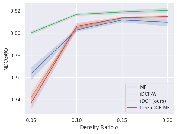
(a)

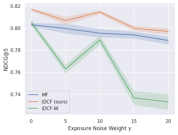
(b)

Figure 4. Recommendation performance on the simulated datasets with different (a) exposure density ratios and (b) exposure noise weights. A larger $\alpha$ means denser user exposure. A larger $\gamma$ means the exposure contains more random noise.

(c) Ground truth.

(d) iDCF (ours).

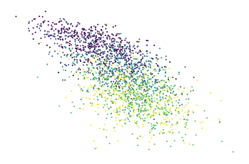
(e) iDCF-W.

Figure 5. The visualization of the true unmeasured confounder and the learned latent confounders using iDCF and iDCF-W. The colors correspond to the user’s feature $\boldsymbol{w}_{u}$.

RQ3: Influence of learning identifiable latent confounders. The synthetic dataset enables us to visualize the true unmeasured confounder and study the influence of the identifiability of the learned confounders on the model performance. Here, we show the identification of the latent confounder by visualization, and conduct experiments to study the robustness of iDCF against different exposure noise weights $\gamma$ with fixed $\alpha=0.1$ and $\beta=2.0$. The empirical results show that our method can better identify the unmeasured confounder, leading to more accurate feedback predictions.

Visualization of the learned latent confounder. Figure 4(c) shows the conditional distributions of the two-dimensional ground truth of the unmeasured confounder $P(\boldsymbol{z}_{u}|\boldsymbol{w}_{u})$ with the exposure noise weight $\gamma=0$. We use iDCF and iDCF-W to learn the corresponding latent confounders, respectively, and we plot the posterior distributions $p(\hat{\boldsymbol{z}}_{u}|\boldsymbol{a}_{u},\boldsymbol{w}_{u})$ and $p(\hat{\boldsymbol{z}}_{u}|\boldsymbol{a}_{u})$ in Figures 4(d) and 4(e). It can be shown that iDCF can identify a better latent confounder than iDCF-W does, which helps to explain the observation that iDCF is better than iDCF-W in previous experiments.

Impact of the exposure noise on the learned confounder. Next, we vary the exposure noise weight $\gamma$ to study the impact of the $\gamma$ on the learned latent confounder. The intuition behind this experiment is that as the weight of the noise increases, there will be more randomness in the exposure vectors, making it more challenging to infer the unmeasured confounders.

To assess the accuracy of the learned confounders in approximating the ground truth, we compute the mean correlation coefficients (MCC) between the learned confounders and the ground truth. MCC is a widely accepted metric in the literature for evaluating the identifiability of learned latent variables (Khemakhem et al., 2020). The results are presented in Table 4. As observed in the table, the results suggest that as the noise level increases, it becomes increasingly difficult to approximate the ground truth using the learned confounders, while iDCF is much more robust regarding to the increasing noise level, compared to iDCF-W.

Table 4. The mean correlation coefficients (MCC) between the true confounder and the latent confounders learned by iDCF and iDCF-W model. A larger MCC means a larger correlation with the true unmeasured confounder.

Model	$\gamma=0.$	$\gamma=5.0$	$\gamma=10.0$	$\gamma=15.0$	$\gamma=20.0$
iDCF-W	$0.6050$	$0.3374$	$0.1023$	$0.1001$	$0.0682$
iDCF (ours)	$0.8394$	$0.8052$	$0.6955$	$0.6914$	$0.6062$

Impact of exposure noise on the feedback prediction. Moreover, we conduct experiments to investigate how the performance of iDCF varies with the exposure noise weight $\gamma$. We choose MF and iDCF-W as the baselines because (1) MF is an empirically stable recommendation model and (2) iDCF-W is the same as iDCF except it does not guarantee the identifiability of the learned confounders. We report NDCG@5 in Figure 4(b). The results indicate that, in general, as the exposure noise increases, it becomes more challenging to identify latent confounders, which in turn makes it more difficult to predict counterfactual feedback. These results, along with those in Table 4, show that a better approximation of the ground truth confounders often leads to better estimation of the true user feedback.

6. conclusion and future work

In this work, we studied how to identify the user’s counterfactual feedback by mitigating the unmeasured confounding bias in recommendation systems. We highlight the importance of identification of the user’s counterfactual feedback by showing the non-identification issue of the Deconfounder method, which can finally lead to inconsistent feedback prediction. To this end, we propose a general recommendation framework that utilizes proximal causal inference to address the non-identification issue and provide theoretical guarantees for mitigating the bias caused by unmeasured confounders. We conduct extensive experiments to show the effectiveness and robustness of our methods in real-world datasets and synthetic datasets.

This work leverages proxy variables to infer the unmeasured confounder and users’ feedback. In the future, we are interested in trying more feasible proxy variables (e.g., item features) and how to combine different proxy variables to achieve better performance. It also makes sense to apply our framework to sequential recommendations and other downstream recommendation scenarios (e.g., solving the challenge of filter bubbles).

Appendix A Algorithm

Input : $\{\boldsymbol{a}_{u},\textbf{w}_{u}\},\forall u\in\mathcal{U}$, $\{r_{ui}\},\forall(u,i)\in\mathcal{D}$

1 Training phase:

// Learning Latent Confounder

2

3Calculate the latent confounder distribution $q_{\phi}(\hat{\boldsymbol{z}}_{u}|\boldsymbol{a}_{u},\textbf{w}_{u})$ for each user $u$ by maximizing Eq. 11;

4

// Feedback with given latent confounder

5

6Initialize a recommendation model $f(u,i,\hat{\boldsymbol{z}}_{u};\eta)$ with parameters $\eta$;

7 while Stop condition is not reached do

8       Fetch $(u,i)$ from $\mathcal{D}$;

9       Minimize the loss Eq. 14 to optimize $\eta$;

10 end while

11Inference phase:

Calculate the prediction of user’s feedback $\hat{r}_{ui}$ according to Eq. 15 for each $(u,i)$ pair.

Algorithm 1 Identifiable Deconfounder (iDCF)

Appendix B Experiment Details

Data Generation Process. The simulated dataset consists of 2,000 users and 300 items. For each user $u$, the unmeasured confounder $\boldsymbol{z}_{u}$ is a two-dimensional representation of the user’s socio-economic status sampled from a mixture of five independent multivariate Gaussian distributions. The proxy variable $w_{u}\in\{1,2,3,4,5\}$ is a one-dimensional categorical variable indicating the user’s consumption level, which is determined by $\boldsymbol{z}_{u}$ such that the prior of $w_{u}$ is uniformly distributed and the conditional distribution of $\boldsymbol{z}_{u}$ follows:

(16) $$\boldsymbol{z}_{u}^{k}|w_{u}\sim N(\mu_{k}(w_{u}),\sigma_{k}^{2}(w_{u})),k\in\{1,2\},$$

where ${\boldsymbol{z}_{u}}^{k}$ is the j-th element of $\boldsymbol{z}_{u}$.

The exposure of the pair $(u,i)$ is generated by

(17) $$\begin{split}&a_{ui}\sim Bernoulli(g_{i}(\boldsymbol{z}_{u})),\\ &g_{i}(\boldsymbol{z})=\alpha\cdot sigmoid(LeakyRelu(\boldsymbol{z}\boldsymbol{M}e_{zi})+\gamma\epsilon)\end{split}$$

where $M$ is a $2\times 2$ matrix, and each element of $M$ is sampled from a uniform distribution. $e_{zi}$ is a randomly generated item-wise 2-dimensional embedding vector, $\alpha$ is a hyper-parameter that controls the sparsity of the exposure vector $\boldsymbol{a}_{u}$, $\epsilon$ is random noise, and $\gamma$ is the corresponding weight of the noise.

The true feedback of user $u$ on item $i$ is $r_{ui}=f_{n}(e_{u}^{T}e_{i}+\beta z_{u}^{T}e_{zi}+\epsilon_{ui})$, where $f_{n}:\mathbb{R}\to\{1,2,3,4,5\}$ is a normalization function, $\epsilon_{ui}$ is an i.i.d. random noise, and $\beta$ is a hyper-parameter controlling the weight of the confounding effect.

Implementation Details.

Outcome Model. Our method is model-agnostic in the sense that it works with any outcome prediction model. For ease of comparison, we follow the recent work on unmeasured confounders (Wang et al., 2020), and adopt matrix factorization (MF) as the backbone model. Specifically, we take $f(u,i,\hat{\boldsymbol{z}}_{u};\eta)=f_{1}(u,i)+f_{2}(\hat{\boldsymbol{z}}_{u},i)$ in Eq. 14, where

(18) $$f_{1}(u,i)=\textbf{e}_{u}^{T}\textbf{e}_{i}+b_{u}+b_{i},f_{2}(\hat{\boldsymbol{z}}_{u},i)=\hat{\boldsymbol{z}}_{u}^{T}\textbf{c}_{i},$$

where $\textbf{e}_{i},\textbf{c}_{i}$ are different embeddings of item $i$, $\textbf{e}_{u}$ is embedding representation of user $u$, $b_{u},b_{i}$ are the user preference bias term and item preference bias term, respectively. During training, $\hat{\boldsymbol{z}}_{u}$ is sampled from $q_{\phi}(\hat{\boldsymbol{z}}_{u}|\boldsymbol{a}_{u},\boldsymbol{w}_{u})$ to approximate the integral in Eq. 9.

In the inference phase, we direct take $\bar{\boldsymbol{z}}_{u}=E_{q_{\phi}(\hat{\boldsymbol{z}}_{u}|\boldsymbol{a}_{u},\boldsymbol{w}_{u})}[\hat{\boldsymbol{z}}_{u}]$ and estimate the user’s feedback on item $i$ as follows:

(19) $$\hat{r}_{ui}=\textbf{e}_{u}^{T}\textbf{e}_{i}+\bar{\boldsymbol{z}}_{u}^{T}\textbf{c}_{i}+b_{u}+b_{i}.$$

Hyper-parameter search. For all recommendation models, we use grid search to select the hyper-parameters based on the model’s performance on the validation dataset. The learning rate is searched from {1e-3, 5e-4, 1e-4, 5e-5, 1e-5}, and the weight decay is chosen from {1e-5, 1e-6}. We adopt their codes for the baselines with public implementation and follow the suggested range of hyper-parameters. The public implementation of IPS and RD-IPS (Ding et al., 2022) relies on a small set of unbiased data to obtain the propensity scores, we follow their procedure and extract the same proportion of unbiased data from the validation set. For a fair comparison, we use ADAM (Kingma and Ba, 2014) for the optimization of all models.

Evaluation Metrics are $NDCG@K$ and $Recall@K$. We report the average value and standard deviation for each method with $10$ different random seeds. The p-value of the T-test between our method and the best baseline is also reported.

Appendix C Supplementary Proof

Proof of Lemma 4.2.

There are 4 unknown values $\{p_{zr|a},z,r\in\{0,1\}\}$ with 4 linear constraints:

(20) $$\begin{array}[]{ll}(1)\sum_{z}\sum_{r}p_{zr|\boldsymbol{a}}=1,&(2)\sum_{z}p_{z1|\boldsymbol{a}}\frac{\pi_{\hat{z}_{u}=z|\boldsymbol{a},w=1}}{\pi_{\hat{z}_{u}=z|\boldsymbol{a}}}=\pi_{r_{ui}=1|\boldsymbol{a},w=1},\\ (3)\sum_{r}p_{1r|\boldsymbol{a}}=\pi_{\hat{z}_{u}=1|\boldsymbol{a}},&(4)\sum_{z}p_{z1|a}\frac{\pi_{\hat{z}_{u}=z|\boldsymbol{a},w=0}}{\pi_{\hat{z}_{u}=z|\boldsymbol{a}}}=\pi_{r_{ui}=1|\boldsymbol{a},w=0}.\end{array}$$

By solving (1) and (3):

(21) $$p_{10}=\pi_{\hat{z}_{u}=1|\boldsymbol{a}}-p_{11},p_{00}=1-p_{01}-\pi_{\hat{z}_{u}=1|\boldsymbol{a}}.$$

Then it remains to solve $p_{01}$ and $p_{11}$ from (2) and (4). and the unique solution from (2) and (4) requires that

(22) $$\begin{split}\frac{\pi_{\hat{z}_{u}=0|\boldsymbol{a},w=1}}{\pi_{\hat{z}_{u}=0|\boldsymbol{a}}}\frac{\pi_{\hat{z}_{u}=1|\boldsymbol{a},w=0}}{\pi_{\hat{z}_{u}=1|\boldsymbol{a}}}-\frac{\pi_{\hat{z}_{u}=1|\boldsymbol{a},w=1}}{\pi_{\hat{z}_{u}=1|\boldsymbol{a}}}\frac{\pi_{\hat{z}_{u}=0|\boldsymbol{a},w=0}}{\pi_{\hat{z}_{u}=0|\boldsymbol{a}}}&\neq 0\\ \pi_{\hat{z}_{u}=1|\boldsymbol{a},w=1}(1-\pi_{\hat{z}_{u}=1|\boldsymbol{a},w=0})-\pi_{\hat{z}_{u}=1|\boldsymbol{a},w=0}(1-\pi_{\hat{z}_{u}=0|\boldsymbol{a},w=1})&\neq 0\\ \pi_{\hat{z}_{u}=1|\boldsymbol{a},w=1}-\pi_{\hat{z}_{u}=1|\boldsymbol{a},w=0}&\neq 0.\end{split}$$

Since $w_{u}$ is assumed to be correlated with $z_{u}$ condition on $\boldsymbol{a}$, and $\hat{z}_{u}$ is learned from the unique factorization $p(\boldsymbol{a}_{u})$, which means $\hat{z}_{u}$ is also correlated with $w_{u}$ condition on $\boldsymbol{a}$.

Therefore, the condition in Eq. 22 is satisfied, i.e., $\{p_{zr|a},z,r\in\{0,1\}\}$ have a unique solution. And $r_{ui}^{\boldsymbol{a}}$ is also uniquely determined by Eq. 2.

∎

References

- (1)
- Arjovsky et al. (2019) Martin Arjovsky, Léon Bottou, Ishaan Gulrajani, and David Lopez-Paz. 2019. Invariant risk minimization. arXiv preprint arXiv:1907.02893 (2019).
- Bühlmann (2020) Peter Bühlmann. 2020. Invariance, causality and robustness. Statist. Sci. 35, 3 (2020), 404–426.
- D’Amour (2019) Alexander D’Amour. 2019. On multi-cause causal inference with unobserved confounding: Counterexamples, impossibility, and alternatives. arXiv preprint arXiv:1902.10286 (2019).
- Ding et al. (2022) Sihao Ding, Peng Wu, Fuli Feng, Yitong Wang, Xiangnan He, Yong Liao, and Yongdong Zhang. 2022. Addressing Unmeasured Confounder for Recommendation with Sensitivity Analysis. In Proceedings of the 28th ACM SIGKDD Conference on Knowledge Discovery and Data Mining (Washington DC, USA) (KDD ’22). Association for Computing Machinery, New York, NY, USA, 305–315. https://doi.org/10.1145/3534678.3539240
- Gao et al. (2022) Chongming Gao, Shijun Li, Yuan Zhang, Jiawei Chen, Biao Li, Wenqiang Lei, Peng Jiang, and Xiangnan He. 2022. KuaiRand: An Unbiased Sequential Recommendation Dataset with Randomly Exposed Videos. In Proceedings of the 31st ACM International Conference on Information & Knowledge Management. 3953–3957.
- Grimmer et al. (2020) Justin Grimmer, Dean Knox, and Brandon M Stewart. 2020. Na” ive regression requires weaker assumptions than factor models to adjust for multiple cause confounding. arXiv preprint arXiv:2007.12702 (2020).
- He et al. (2022) Xiangnan He, Yang Zhang, Fuli Feng, Chonggang Song, Lingling Yi, Guohui Ling, and Yongdong Zhang. 2022. Addressing Confounding Feature Issue for Causal Recommendation. arXiv preprint arXiv:2205.06532 (2022).
- Hernán and Robins (2010) Miguel A Hernán and James M Robins. 2010. Causal inference.
- Khemakhem et al. (2020) Ilyes Khemakhem, Diederik Kingma, Ricardo Monti, and Aapo Hyvarinen. 2020. Variational autoencoders and nonlinear ica: A unifying framework. In International Conference on Artificial Intelligence and Statistics. PMLR, 2207–2217.
- Kingma and Ba (2014) Diederik P Kingma and Jimmy Ba. 2014. Adam: A method for stochastic optimization. arXiv preprint arXiv:1412.6980 (2014).
- Kingma and Welling (2013) Diederik P Kingma and Max Welling. 2013. Auto-encoding variational bayes. arXiv preprint arXiv:1312.6114 (2013).
- Koren et al. (2009) Yehuda Koren, Robert Bell, and Chris Volinsky. 2009. Matrix factorization techniques for recommender systems. Computer 42, 8 (2009), 30–37.
- Kruskal (1989) J. B. Kruskal. 1989. Rank, Decomposition, and Uniqueness for 3-Way and n-Way Arrays. North-Holland Publishing Co., NLD, 7–18.
- Kuroki and Pearl (2014) Manabu Kuroki and Judea Pearl. 2014. Measurement bias and effect restoration in causal inference. Biometrika 101, 2 (2014), 423–437.
- Liu et al. (2022) Haochen Liu, Da Tang, Ji Yang, Xiangyu Zhao, Hui Liu, Jiliang Tang, and Youlong Cheng. 2022. Rating Distribution Calibration for Selection Bias Mitigation in Recommendations. In Proceedings of the ACM Web Conference 2022 (Virtual Event, Lyon, France) (WWW ’22). Association for Computing Machinery, New York, NY, USA, 2048–2057. https://doi.org/10.1145/3485447.3512078
- Miao et al. (2018a) Wang Miao, Zhi Geng, and Eric J Tchetgen Tchetgen. 2018a. Identifying causal effects with proxy variables of an unmeasured confounder. Biometrika 105, 4 (2018), 987–993.
- Miao et al. (2022) Wang Miao, Wenjie Hu, Elizabeth L Ogburn, and Xiao-Hua Zhou. 2022. Identifying effects of multiple treatments in the presence of unmeasured confounding. J. Amer. Statist. Assoc. (2022), 1–15.
- Miao et al. (2018b) Wang Miao, Xu Shi, and Eric Tchetgen Tchetgen. 2018b. A confounding bridge approach for double negative control inference on causal effects. arXiv preprint arXiv:1808.04945 (2018).
- Mondal et al. (2022) Abhirup Mondal, Anirban Majumder, and Vineet Chaoji. 2022. ASPIRE: Air Shipping Recommendation for E-Commerce Products via Causal Inference Framework. In Proceedings of the 28th ACM SIGKDD Conference on Knowledge Discovery and Data Mining (Washington DC, USA) (KDD ’22). Association for Computing Machinery, New York, NY, USA, 3584–3592. https://doi.org/10.1145/3534678.3539197
- Pearl (2009) Judea Pearl. 2009. Causality: Models, Reasoning and Inference (2nd ed.). Cambridge University Press.
- Robins (1986) James Robins. 1986. A new approach to causal inference in mortality studies with a sustained exposure period—application to control of the healthy worker survivor effect. Mathematical Modelling 7, 9 (1986), 1393–1512. https://doi.org/10.1016/0270-0255(86)90088-6
- Rubin (1974) Donald B Rubin. 1974. Estimating causal effects of treatments in randomized and nonrandomized studies. Journal of educational Psychology 66, 5 (1974), 688.
- Schnabel et al. (2016) Tobias Schnabel, Adith Swaminathan, Ashudeep Singh, Navin Chandak, and Thorsten Joachims. 2016. Recommendations as treatments: Debiasing learning and evaluation. In international conference on machine learning. PMLR, 1670–1679.
- Si et al. (2022) Zihua Si, Xueran Han, Xiao Zhang, Jun Xu, Yue Yin, Yang Song, and Ji-Rong Wen. 2022. A Model-Agnostic Causal Learning Framework for Recommendation using Search Data. In Proceedings of the ACM Web Conference 2022. 224–233.
- Strang et al. (1993) Gilbert Strang, Gilbert Strang, Gilbert Strang, and Gilbert Strang. 1993. Introduction to linear algebra. Vol. 3. Wellesley-Cambridge Press Wellesley, MA.
- Tchetgen et al. (2020) Eric J Tchetgen Tchetgen, Andrew Ying, Yifan Cui, Xu Shi, and Wang Miao. 2020. An introduction to proximal causal learning. arXiv preprint arXiv:2009.10982 (2020).
- Wang et al. (2021) Wenjie Wang, Fuli Feng, Xiangnan He, Xiang Wang, and Tat-Seng Chua. 2021. Deconfounded recommendation for alleviating bias amplification. In Proceedings of the 27th ACM SIGKDD Conference on Knowledge Discovery & Data Mining. 1717–1725.
- Wang and Blei (2019) Yixin Wang and David M Blei. 2019. The blessings of multiple causes. J. Amer. Statist. Assoc. 114, 528 (2019), 1574–1596.
- Wang et al. (2020) Yixin Wang, Dawen Liang, Laurent Charlin, and David M Blei. 2020. Causal inference for recommender systems. In Fourteenth ACM Conference on Recommender Systems. 426–431.
- Wang et al. (2022) Zimu Wang, Yue He, Jiashuo Liu, Wenchao Zou, Philip S Yu, and Peng Cui. 2022. Invariant Preference Learning for General Debiasing in Recommendation. In Proceedings of the 28th ACM SIGKDD Conference on Knowledge Discovery and Data Mining. 1969–1978.
- Wei et al. (2021) Tianxin Wei, Fuli Feng, Jiawei Chen, Ziwei Wu, Jinfeng Yi, and Xiangnan He. 2021. Model-agnostic counterfactual reasoning for eliminating popularity bias in recommender system. In Proceedings of the 27th ACM SIGKDD Conference on Knowledge Discovery & Data Mining. 1791–1800.
- Wu et al. (2022) Le Wu, Xiangnan He, Xiang Wang, Kun Zhang, and Meng Wang. 2022. A survey on accuracy-oriented neural recommendation: From collaborative filtering to information-rich recommendation. IEEE Transactions on Knowledge and Data Engineering (2022).
- Xu et al. (2021) Shuyuan Xu, Juntao Tan, Shelby Heinecke, Jia Li, and Yongfeng Zhang. 2021. Deconfounded Causal Collaborative Filtering. arXiv preprint arXiv:2110.07122 (2021).
- Zhan et al. (2022) Ruohan Zhan, Changhua Pei, Qiang Su, Jianfeng Wen, Xueliang Wang, Guanyu Mu, Dong Zheng, Peng Jiang, and Kun Gai. 2022. Deconfounding Duration Bias in Watch-time Prediction for Video Recommendation. In Proceedings of the 28th ACM SIGKDD Conference on Knowledge Discovery and Data Mining. 4472–4481.
- Zhang et al. (2021) Yang Zhang, Fuli Feng, Xiangnan He, Tianxin Wei, Chonggang Song, Guohui Ling, and Yongdong Zhang. 2021. Causal intervention for leveraging popularity bias in recommendation. In Proceedings of the 44th International ACM SIGIR Conference on Research and Development in Information Retrieval. 11–20.
- Zhou et al. (2018) Guorui Zhou, Xiaoqiang Zhu, Chenru Song, Ying Fan, Han Zhu, Xiao Ma, Yanghui Yan, Junqi Jin, Han Li, and Kun Gai. 2018. Deep interest network for click-through rate prediction. In Proceedings of the 24th ACM SIGKDD international conference on knowledge discovery & data mining. 1059–1068.
- Zhu et al. (2022b) Xinyuan Zhu, Yang Zhang, Fuli Feng, Xun Yang, Dingxian Wang, and Xiangnan He. 2022b. Mitigating Hidden Confounding Effects for Causal Recommendation. arXiv preprint arXiv:2205.07499 (2022).
- Zhu et al. (2022a) Yaochen Zhu, Jing Yi, Jiayi Xie, and Zhenzhong Chen. 2022a. Deep causal reasoning for recommendations. arXiv preprint arXiv:2201.02088 (2022).