Federated Auto-weighted Domain Adaptation

Abstract

Federated Domain Adaptation (FDA) describes the federated learning setting where a set of source clients work collaboratively to improve the performance of a target client where limited data is available. The domain shift between the source and target domains, coupled with sparse data in the target domain, makes FDA a challenging problem, e.g., common techniques such as FedAvg and fine-tuning, often fail with the presence of significant domain shift and data scarcity. To comprehensively understand the problem, we introduce metrics that characterize the FDA setting and put forth a theoretical framework for analyzing the performance of aggregation rules. We also propose a novel aggregation rule for FDA, Federated Gradient Projection (FedGP), used to aggregate the source gradients and target gradient during training. Importantly, our framework enables the development of an auto-weighting scheme that optimally combines the source and target gradients. This scheme improves both FedGP and a simpler heuristic aggregation rule (FedDA). Experiments on synthetic and real-world datasets verify the theoretical insights and illustrate the effectiveness of the proposed method in practice.

1 Introduction

Federated learning (FL) is a distributed machine learning paradigm that aggregates clients’ models on the server while maintaining data privacy [22]. This method is particularly pertinent in real-world scenarios where data heterogeneity and insufficiency are common issues, such as in healthcare settings. For instance, a small local hospital may struggle to train a generalizable model independently due to insufficient data, and the domain divergence from other hospitals further complicates the application of FL. These challenges give rise to a problem known as Federated Domain Adaptation (FDA), where source clients collaborate to enhance the model performance of a target client. FDA presents a considerable hurdle due to two primary factors: (i) the domain shift existing between source and target domains, and (ii) the scarcity of data in the target domain.

Recent studies have endeavored to address the challenges related to FDA. A portion of these works aims to minimize the impacts of distribution shifts between clients [27, 13, 31], with some focusing on personalized federated learning [6, 18, 4, 21]. However, these studies commonly presume that all clients possess an ample amount of data, an assumption that may not hold true in real-world scenarios. An alternative approach is Unsupervised Federated Domain Adaptation (UFDA) [24, 8, 28], useful when there is abundant unlabeled data within the target domain. Nonetheless, there remains an under-explored gap when both primary challenges, domain shift and data scarcity, coexist.

To fill the gap, this work takes a direct approach to the two principal challenges associated with FDA by carefully designing federated aggregation rules. Perhaps surprisingly, we discover that even noisy gradients, computed using the limited data of the target client, can still deliver a valuable signal. To this end, we anchor our work on a critical question that we aim to answer rigorously. This question forms the backbone of our investigation and guides our exploration into the realm of the FDA.

How do we define a “good” FDA aggregation rule?

To our best understanding, there are currently no theoretical foundations that systematically examine the behaviors of various federated aggregation rules within the context of the FDA. Therefore, to rigorously address the aforementioned question, we introduce a theoretical framework. This framework formally establishes two metrics designed to capture the distinct characteristics of specific FDA settings and employs these metrics to analyze the performance of FDA aggregation rules. The proposed metrics characterize (i) the divergence between source and target domains and (ii) the level of training data scarcity in the target domain. Together, these metrics formally characterize FDA.

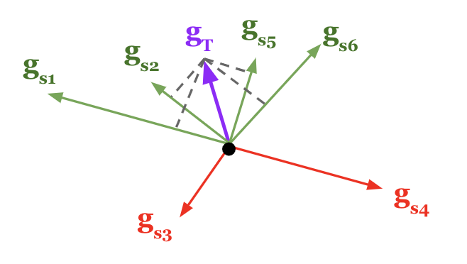
Figure 1: FedGP filters out the negative gradients (colored in red) and convexly combines $g_{T}$ and its projections to the directions of the remaining source gradients (green ones).

Leveraging the proposed theoretical framework, we analyze two aggregation approaches. The first is a simple heuristic FedDA, a simple weighted average of the source and target gradients. The second is a novel filtering-based gradient projection method, FedGP. This method is designed to extract and aggregate beneficial components of the source gradients with the assistance of the target gradient, as depicted in Figure 1. FedGP calculates a convex combination of the target gradient and its positive projection along the direction of source gradients. We find that performing the projection operation prior to the convex combination is crucial. Our experimental results show that a naive convex combination of source and target gradients (i.e., FedDA) sometimes is ineffective. Intriguingly, our theoretical framework unravels the reasons why FedGP may outperform FedDA.

Finally, our theoretical framework suggests the optimal weight parameters for combining source and target gradients. Therefore, we present auto-weighted versions of both FedGP and FedDA to further improve their performance. We conduct synthetic experiments that affirm the practical predictive power of our theoretical framework. Notably, we find that while FedGP is less sensitive to re-weighting with relatively good performance for $\beta=0.5$, the under-performing FedDA is significantly improved by using auto-weighting - enough to be competitive with FedGP, demonstrating the value of our proposed methodology. Across three real-world datasets, we demonstrate that FedGP, as well as the auto-weighted FedDA and FedGP, yield strong performance compared to various benchmarks.

Summary of Contributions.

• We introduce a theoretical framework for analyzing the performance of FDA aggregation rules, which may be of broader interest. Within this framework, we provide a theoretical response to the pivotal question: How do we define a “good” FDA aggregation rule?

• We propose FedGP as an effective solution to FDA challenges characterized by substantial domain shifts and limited target data.

• Our theoretical framework facilitates the creation of auto-weighted versions of the aggregation rules, FedDA and FedGP, leading to further performance enhancement.

• Extensive experiments illustrate that our theory is predictive of practice and that the proposed methods are effective on real-world datasets.

Paper Structure. In Section 2 we introduce the problem of federated domain adaptation in a general manner. In Section 3 we propose our theoretical framework as a formal definition of the problem, providing tools for understanding the problem mathematically. To solve the problem of FDA, in Section 4 we propose and theoretically investigate two methods (FedDA and FedGP), and therefore their auto-weighted versions. We empirically investigate the proposed methods and prior work in Section 5&6. All proofs are deferred to the Appendix A.1.

2 The Problem of Federated Domain Adaptation

In this section, we initiate our discussion by presenting a general definition of the problem of Federated Domain Adaptation and subsequently a review of related literature in the field.

Notation. Let ${\mathcal{D}}$ be a data domain on a ground set ${\mathcal{Z}}$. In our supervised setting, a data point $z\in{\mathcal{Z}}$ is the tuple of input and output data. We denote the loss function as $\ell:\Theta\times{\mathcal{Z}}\to{\mathbb{R}}$ where the parameter space is $\Theta={\mathbb{R}}^{m}$; an $m$-dimensional Euclidean space. The population loss is $\ell_{\mathcal{D}}(\theta):=\mathbb{E}_{z\sim{\mathcal{D}}}\ell(\theta,z)$, where $\mathbb{E}_{z\sim{\mathcal{D}}}$ is the expectation w.r.t. ${\mathcal{D}}$. Let $\widehat{\mathcal{D}}$ be a finite sample dataset drawn from ${\mathcal{D}}$, then $\ell_{\widehat{\mathcal{D}}}(\theta):=\tfrac{1}{|\widehat{\mathcal{D}}|}\sum_{z\in\widehat{\mathcal{D}}}\ell(\theta,z)$, where $|\widehat{\mathcal{D}}|$ is the size of the dataset. We use $[N]:=\{1,2,\dots,N\}$. By default, $\langle\cdot,\cdot\rangle$, and $\|\cdot\|$ respectively denote the Euclidean inner product and Euclidean norm.

In FDA, there are $N$ source clients with their respective source domains $\{{\mathcal{D}}_{S_{i}}\}_{i\in[N]}$ and a target client with the target domain ${\mathcal{D}}_{T}$. For $\forall i\in[N]$, the $i^{th}$ source client holds a dataset $\widehat{\mathcal{D}}_{S_{i}}$ and the target client holds a dataset $\widehat{\mathcal{D}}_{T}$. We consider the case that $|\widehat{\mathcal{D}}_{T}|$ is relatively small.

Definition 2.1 (Federated Domain Adaptation (FDA)).

In the problem of FDA, all clients collaborate in a federated manner to improve the global model for the target domain. The global model is trained by iteratively updating the global model parameter

$$\theta\leftarrow\theta-\mu\cdot\texttt{Aggr}(\{\nabla\ell_{\widehat{\mathcal{D}}_{S_{i}}}(\theta)\}_{i\in[n]},\nabla\ell_{\widehat{\mathcal{D}}_{T}}(\theta)),$$ (1)

where $\nabla\ell$ is the gradient, $\mu$ is the step size. Therefore, the problem of FDA is to find a good strategy $\texttt{Aggr}(\cdot)$ such that the global model parameter $\theta$ after training attains a minimized target domain population loss function $\ell_{{\mathcal{D}}_{T}}(\theta)$. Note that $\texttt{Aggr}(\cdot)$ may depend on iteration time steps.

There are a number of challenges that make FDA difficult to solve. First, the amount of labeled data in the target domain is typically limited, which makes it difficult to learn a generalizable model. Second, the source and target domains have different data distributions, which can lead to a mismatch between the features learned by the source and target models. Moreover, the model must be trained in a privacy-preserving manner where local data cannot be shared.

2.1 Related Work

Data heterogeneity, personalization and label deficiency in FL. Distribution shifts between clients remain a crucial challenge in FL. Current work often focuses on improving the aggregation rules: Karimireddy et al., [13] use control variates and Xie et al., 2020b [31] cluster the client weights via EM algorithm to correct the drifts among clients. More recently, there are works [6, 18, 4, 21] concentrating on personalized federated learning by finding a better mixture of local/global models and exploring shared representation. Further, recent works have addressed the label deficiency problem with self-supervision or semi-supervision for personalized models [12, 10, 32]. All existing work often assumes sufficient data for all clients - nevertheless, the performance of a client with data deficiency and large shifts may become unsatisfying (Table 1). Compared to related work on personalized FL, our method is more robust to data scarcity on the target client.

Unsupervised federated domain adaptation. There is a considerable amount of recent work on unsupervised federated domain adaptation (UFDA), with recent highlights in adversarial training [26, 33], knowledge distillation [23], and source-free methods [20]. Peng et al., [24], Li et al., [19] is the first to extend MSDA into an FL setting; they apply adversarial adaptation techniques to align the representations of nodes. More recently, in KD3A [8] and COPA [28], the server with unlabeled target samples aggregates the local models by learning the importance of each source domain via knowledge distillation and collaborative optimization. However, training with unlabeled data every round is computationally expensive, and the signals coming from the unlabeled data are noisy and sometimes misleading. Compared to related work on UFDA, we take a more principled FL perspective where the goal is to find ideal aggregation strategies.

Using additional gradient information in FL. Model updates in each communication round may provide valuable insights into client convergence directions. This idea has been explored for robustness in FL, particularly with untrusted clients. For example, Zeno++ [30] and FlTrust [3] leverage the additional gradient computed from a small clean training dataset on the server to compute the scores of candidate gradients for detecting the malicious adversaries. Differently, our work focus on improving the performance for the target domain with auto-weighted aggregation rules that utilize the gradient signals from all clients.

3 A Theoretical Framework for Analyzing Aggregation Rules for FDA

In this section, we introduce a general framework for analyzing aggregation rules for federated domain adaptation by formulating it into a formal theoretical problem.

Additional Notation and Setting. We use additional notation to motivate a functional view of FDA. Let $g_{\mathcal{D}}:\Theta\to\Theta$ with $g_{\mathcal{D}}(\theta):=\nabla\ell_{\mathcal{D}}(\theta).$ Given a distribution $\pi$ on the parameter space $\Theta$, we define an inner product $\langle g_{\mathcal{D}},g_{{\mathcal{D}}^{\prime}}\rangle_{\pi}=\mathbb{E}_{\theta\sim\pi}[\langle g_{\mathcal{D}}(\theta),g_{{\mathcal{D}}^{\prime}}(\theta)\rangle]$. The inner product induces the $L^{\pi}$-norm on $g_{\mathcal{D}}$ as $\|g_{\mathcal{D}}\|_{\pi}:=\sqrt{\mathbb{E}_{\theta\sim\pi}\|g_{\mathcal{D}}(\theta)\|^{2}}$. Given an aggregation rule $\texttt{Aggr}(\cdot)$, we denote $\widehat{g}_{\texttt{Aggr}}(\theta)=\texttt{Aggr}(\{g_{{\mathcal{D}}_{S_{i}}}(\theta)\}_{i=1}^{N},g_{\widehat{\mathcal{D}}_{T}}(\theta))$. Note that we do not care about the generalization on the source domains, and therefore for the theoretical analysis, we can gladly view ${\mathcal{D}}_{S}=\widehat{\mathcal{D}}_{S}$. Throughout our theoretical analysis, we make the following standard assumption.

Assumption. We assume the target domain’s local dataset $\widehat{\mathcal{D}}_{T}$ is sampled i.i.d. from its underlying target domain distribution ${\mathcal{D}}_{T}$. Note that this implies $\mathbb{E}_{\widehat{\mathcal{D}}_{T}}[g_{\widehat{\mathcal{D}}_{T}}]=g_{{\mathcal{D}}_{T}}$.

Observing Definition 2.1, we can see intuitively that a good aggregation rule should have $g_{\texttt{Aggr}}$ being “close” to the ground-truth target domain gradient $g_{{\mathcal{D}}_{T}}$. From a functional view, we would need a “ruler” to measure the distance between the two functions. We choose the $L^{\pi}$-norm as the “ruler” as it exhibits certain benefits, which we will show later. Before that, we make the following definition.

Definition 3.1 (Delta Error of an aggregation rule Aggr$(\cdot)$).

We define the following squared error term to measure the closeness between $g_{\texttt{Aggr}}$ and $g_{{\mathcal{D}}_{T}}$, i.e.,

$$\Delta^{2}_{\texttt{Aggr}}:=\mathbb{E}_{\widehat{\mathcal{D}}_{T}}\|g_{{\mathcal{D}}_{T}}-\widehat{g}_{\texttt{Aggr}}\|^{2}_{\pi}.$$ (2)

The first benefit of the chosen the $L^{\pi}$-norm is that, being a generalization of the $L^{2}$-norm, it can be computed by sampling from the distribution $\pi$. More importantly, one expects an aggregation rule with a small Delta error with the $L^{\pi}$-norm to perform better as measured by the population target domain loss function $\ell_{g_{{\mathcal{D}}_{T}}}$, as we show in the following theorem.

Theorem 3.2.

Consider model parameter $\theta\sim\pi$ and an aggregation rule Aggr$(\cdot)$ with step size $\mu>0$. Define the updated parameter as

$$\theta^{+}:=\theta-\mu\widehat{g}_{\texttt{Aggr}}(\theta).$$ (3)

Assuming the gradient $\nabla\ell(\theta,z)$ is $\gamma$-Lipschitz in $\theta$ for any $z$, and let the step size $\mu=\tfrac{1}{\gamma},$ we have

$$\mathbb{E}_{\widehat{\mathcal{D}}_{T},\theta}[\ell_{{\mathcal{D}}_{T}}(\theta^{+})-\ell_{{\mathcal{D}}_{T}}(\theta)]\leq-\tfrac{1}{2\gamma}(\|g_{{\mathcal{D}}_{T}}\|_{\pi}^{2}-\Delta^{2}_{\texttt{Aggr}}).$$ (4)

We note that the choice of step size is mainly to improve the readability of the theorem. A generalized version of the theorem is provided in the Appendix A.1, where we relax the condition on the step size.

The distribution $\pi$ characterizes where in the model parameter space we want to measure the gradients. In other words, the above theorem answers the following question: for a random parameter sampled from $\pi$, a distribution of model parameters over training, how much does a certain aggregation improve the performance of one step of gradient descent? This is crucial information, as it characterizes the convergence quality for each aggregation rule.

To analyze an aggregation rule, it is further necessary to characterize the specific FDA setting. For example, the behavior of an aggregation rule varies with the degree and nature of source-target domain shift and labeled sample size in the target domain. To characterize the source-target domain distance, given a source domain ${\mathcal{D}}_{S}$, we can similarly measure its distance to the target domain ${\mathcal{D}}_{T}$ as the $L^{\pi}$-norm distance between $g_{{\mathcal{D}}_{S}}$ and the target domain model ground-truth gradient $g_{{\mathcal{D}}_{T}}$.

Definition 3.3 ($L^{\pi}$ Source-Target Domain Distance).

Given a source domain ${\mathcal{D}}_{S}$, its distance to the target domain ${\mathcal{D}}_{T}$ is defined as

$$d_{\pi}({\mathcal{D}}_{S},{\mathcal{D}}_{T}):=\|g_{{\mathcal{D}}_{T}}-g_{{\mathcal{D}}_{S}}\|_{\pi}.$$ (5)

This proposed metric $d_{\pi}$ has some properties inherited from the norm, including: (i. symmetry) $d_{\pi}({\mathcal{D}}_{S},{\mathcal{D}}_{T})=d_{\pi}({\mathcal{D}}_{T},{\mathcal{D}}_{S})$; (ii, triangle inequality) For any data distribution ${\mathcal{D}}$ we have $d_{\pi}({\mathcal{D}}_{S},{\mathcal{D}}_{T})\leq d_{\pi}({\mathcal{D}}_{S},{\mathcal{D}})+d_{\pi}({\mathcal{D}}_{T},{\mathcal{D}})$; (iii. zero property) For any ${\mathcal{D}}$ we have $d_{\pi}({\mathcal{D}},{\mathcal{D}})=0$.

To formalize the target domain sample size, we again measure the distance between $\widehat{\mathcal{D}}_{T}$ and ${\mathcal{D}}_{T}$. Accordingly, its mean squared error characterizes the amount of samples as a target domain variance.

Definition 3.4 ($L^{\pi}$ Target Domain Variance).

Given the target domain ${\mathcal{D}}_{T}$ and a sampled dataset $\widehat{\mathcal{D}}_{T}$, the target domain variance is defined as

$$\sigma_{\pi}^{2}(\widehat{\mathcal{D}}_{T}):=\mathbb{E}_{\widehat{\mathcal{D}}_{T}}\|g_{{\mathcal{D}}_{T}}-g_{\widehat{\mathcal{D}}_{T}}\|^{2}_{\pi}.$$ (6)

As we can see, $\widehat{\mathcal{D}}_{T}\to{\mathcal{D}}_{T}$ with increasing sample size, resulting in a corresponding decrease in $\sigma^{2}({\mathcal{D}}_{T})$. Therefore, the proposed $\sigma^{2}({\mathcal{D}}_{T})$ characterizes the amount of samples on the target domain.

With the relevant quantities defined, we can form a more formal and concise definition of FDA which answers the pivotal question of how do we define a "good" aggregation rule.

Definition 3.5 (A Formal Formulation of FDA).

Given the target domain variance $\sigma_{\pi}^{2}(\widehat{\mathcal{D}}_{T})$ and source-target domain distances $\forall i\in[N]:d_{\pi}({\mathcal{D}}_{S_{i}},{\mathcal{D}}_{T})$, the problem of FDA is to find a good strategy $\texttt{Aggr}(\cdot)$ such that its Delta error $\Delta^{2}_{\texttt{Aggr}}$ is minimized.

The Theoretical Framework for FDA. Therefore, the above definitions give a powerful framework for analyzing and designing aggregation rules. Concretely,

• given an aggregation rule, we can derive its Delta error and see how it would perform given a FDA setting (as characterized by the target domain variance and the source-target distances);

• given a FDA setting, we can design aggregation rules to minimize the Delta error.

4 Auto-weighted Aggregation Rules for FDA

The framework as presented in the previous section does not reveal a concrete way in designing aggregation rules. Therefore, to gain intuition, we may try using it for two simple cases, i.e., only using the target gradient and only using a source gradient (e.g., the $i^{th}$ source domain). The Delta error of two of the baseline aggregation rules is straightforward. By definition, we have that

$$\Delta^{2}_{\widehat{\mathcal{D}}_{T}\texttt{ only}}=\sigma_{\pi}^{2}(\widehat{\mathcal{D}}_{T}),\quad\ \text{and}\quad\Delta^{2}_{{\mathcal{D}}_{S_{i}}\texttt{ only}}=d^{2}_{\pi}({\mathcal{D}}_{S_{i}},{\mathcal{D}}_{T}).$$ (7)

This immediate result demonstrates the usefulness of the proposed framework: if $\widehat{g}_{\texttt{Aggr}}$ only uses the target gradient then the error is the target domain variance; if $\widehat{g}_{\texttt{Aggr}}$ only uses a source gradient then the error is the corresponding source-target domain bias. Therefore, a good aggregation method must strike a balance between the bias and variance, i.e., a bias-variance trade-off, and this is precisely what our auto-weighting mechanism does. To achieve this, we first propose two aggregation methods, and then we show how the auto-weighting mechanism is derived.

4.1 The Aggregation Rules: FedDA and FedGP

A straightforward way to strike a balance between the source-target bias and the target domain variance is to convexly combine them, as defined in the following.

Definition 4.1 (FedDA).

For each source domains $\forall i\in[N]$ let $\alpha_{i}\in[0,1]$ be weights with $\sum_{i=1}^{N}\alpha_{i}=1$ which balance among the source domains. Moreover, let $\beta_{i}\in[0,1]$ be the weight that balances between the $i^{th}$ source domain and the target domain. The FedDA aggregation operation is

$$\texttt{FedDA}(\{g_{{\mathcal{D}}_{S_{i}}}(\theta)\}_{i=1}^{N},g_{\widehat{\mathcal{D}}_{T}}(\theta))=\sum_{i=1}^{N}\alpha_{i}\left((1-\beta_{i})g_{\widehat{\mathcal{D}}_{T}}(\theta)+\beta_{i}g_{{\mathcal{D}}_{S_{i}}}(\theta)\right).$$ (8)

We can see the benefits of the FedDA aggregation by examining its Delta error.

Theorem 4.2.

Consider FedDA. Given the target domain $\widehat{\mathcal{D}}_{T}$ and $N$ source domains ${\mathcal{D}}_{S_{1}},\dots,{\mathcal{D}}_{S_{N}}$.

$$\Delta^{2}_{\texttt{FedDA}}\leq\sum_{i=1}^{N}\alpha_{i}\Delta^{2}_{\texttt{FedDA},S_{i}},\quad\text{where }\ \Delta^{2}_{\texttt{FedDA},S_{i}}=(1-\beta_{i})^{2}\sigma_{\pi}^{2}(\widehat{\mathcal{D}}_{T})+\beta_{i}^{2}d^{2}_{\pi}({\mathcal{D}}_{S_{i}},{\mathcal{D}}_{T})$$ (9)

is the Delta error when only considering ${\mathcal{D}}_{S_{i}}$ as the source domain.

Therefore, we can see the benefits of combining the source and target domains: with proper choices of weights, $\Delta^{2}_{\texttt{FedDA}}$ can be smaller than the Delta errors of only using any of the domains (equation 7).

We leave the discussion on auto-weighting to a later subsection, as we want to introduce a more interesting aggregation method, FedGP. It shares the same intuition of combining and balancing both the source and target gradients as FedDA, but with an additional step of gradient projection.

Definition 4.3 (FedGP).

For each source domains $\forall i\in[N]$ let $\alpha_{i}\in[0,1]$ be weights with $\sum_{i=1}^{N}\alpha_{i}=1$ which balance among the source domains. Moreover, let $\beta_{i}\in[0,1]$ be the weight that balances between $i^{th}$ source domain and the target domain. The FedGP aggregation operation is

$$\texttt{FedGP}(\{g_{{\mathcal{D}}_{S_{i}}}(\theta)\}_{i=1}^{N},g_{\widehat{\mathcal{D}}_{T}}(\theta))=\sum_{i=1}^{N}\alpha_{i}\left((1-\beta_{i})g_{\widehat{\mathcal{D}}_{T}}(\theta)+\beta_{i}\texttt{Proj}_{+}(g_{\widehat{\mathcal{D}}_{T}}(\theta)|g_{{\mathcal{D}}_{S_{i}}}(\theta))\right).$$ (10)

where $\texttt{Proj}_{+}(g_{\widehat{\mathcal{D}}_{T}}(\theta)|g_{{\mathcal{D}}_{S_{i}}}(\theta))=\max\{\langle g_{\widehat{\mathcal{D}}_{T}}(\theta),g_{{\mathcal{D}}_{S_{i}}}(\theta)\rangle,0\}g_{{\mathcal{D}}_{S_{i}}}(\theta)/\|g_{{\mathcal{D}}_{S_{i}}}(\theta)\|^{2}$ is the operation that projects $g_{\widehat{\mathcal{D}}_{T}}(\theta)$ to the positive direction of $g_{{\mathcal{D}}_{S_{i}}}(\theta)$.

The benefits of FedGP over FedDA are perhaps obscure. Surprisingly, our theoretical framework reveals that the benefits should come from the high dimensionality of the model parameters as follows.

Theorem 4.4.

Consider FedGP. Given the target domain $\widehat{\mathcal{D}}_{T}$ and $N$ source domains ${\mathcal{D}}_{S_{1}},\dots,{\mathcal{D}}_{S_{N}}$.

$$\Delta^{2}_{\texttt{FedGP}}\leq\sum_{i=1}^{N}\alpha_{i}\Delta^{2}_{\texttt{FedGP},S_{i}},\ \text{ where }\Delta^{2}_{\texttt{FedGP},S_{i}}\approx((1-\beta_{i})^{2}+\tfrac{2\beta_{i}-\beta_{i}^{2}}{m})\sigma_{\pi}^{2}(\widehat{\mathcal{D}}_{T})+\beta_{i}^{2}\bar{\tau}^{2}d^{2}_{\pi}({\mathcal{D}}_{S_{i}},{\mathcal{D}}_{T}).$$ (11)

In the above equation, $m$ is the model dimension and $\bar{\tau}^{2}=\mathbb{E}_{\pi}[\tau(\theta)^{2}]\in[0,1]$ where $\tau(\theta)$ is the $\sin(\cdot)$ value of the angle between $g_{{\mathcal{D}}_{S}}(\theta)$ and $g_{{\mathcal{D}}_{T}}(\theta)-g_{{\mathcal{D}}_{S}}(\theta)$.

We note that the approximation is mostly done in analog to the mean-field analysis, and this approximation is accurate enough for auto-weighted FedGP. The rigorous version of the theorem and the specific approximation we make are detailed in Appendix A.1.

Comparing the Delta error of FedGP (equation 11) and that of FedDA (equation 31), we can see that

$$\Delta^{2}_{\texttt{FedDA},S_{i}}-\Delta^{2}_{\texttt{FedGP},S_{i}}\approx\beta_{i}^{2}(1-\bar{\tau}^{2})d^{2}_{\pi}({\mathcal{D}}_{S_{i}},{\mathcal{D}}_{T})-\tfrac{2\beta_{i}-\beta_{i}^{2}}{m}\sigma_{\pi}^{2}(\widehat{\mathcal{D}}_{T}).$$ (12)

In practice, the model dimension $m\gg 1$ while the $\bar{\tau}^{2}<1$, and therefore with the same weights we can expect FedGP to be mostly better than FedDA unless the source-target domain distance is much smaller than the target domain variance.

4.2 The Auto-weighted FedGP and FedDA

Naturally, the above analysis implies a good choice of weighting parameters for either of the methods. Concretely, for each source domains $S_{i}$, we can solve for the optimal $\beta_{i}$ that minimize the corresponding Delta errors, i.e., $\Delta^{2}_{\texttt{FedDA},S_{i}}$ (equation 31) for FedDA and $\Delta^{2}_{\texttt{FedDA},S_{i}}$ (equation 11) for FedGP. Note that for $\Delta^{2}_{\texttt{FedGP},S_{i}}$ we can safely view $\tfrac{2\beta_{i}-\beta_{i}^{2}}{m}\approx 0$ given the high dimensionality of our models. Since either of the Delta errors is quadratic in $\beta_{i}$, they enjoy closed-form solutions:

$$\beta_{i}^{\texttt{FedDA}}=\frac{\sigma_{\pi}^{2}(\widehat{\mathcal{D}}_{T})}{d^{2}_{\pi}({\mathcal{D}}_{S_{i}},{\mathcal{D}}_{T})+\sigma_{\pi}^{2}(\widehat{\mathcal{D}}_{T})},\qquad\beta_{i}^{\texttt{FedGP}}=\frac{\sigma_{\pi}^{2}(\widehat{\mathcal{D}}_{T})}{\bar{\tau}^{2}d^{2}_{\pi}({\mathcal{D}}_{S_{i}},{\mathcal{D}}_{T})+\sigma_{\pi}^{2}(\widehat{\mathcal{D}}_{T})}.$$ (13)

Note that the exact values of $\sigma_{\pi}^{2}(\widehat{\mathcal{D}}_{T}),d^{2}_{\pi}({\mathcal{D}}_{S_{i}},\bar{\tau}^{2}$ are unknown, since they would require knowing the ground-truth target domain gradient $g_{{\mathcal{D}}_{T}}$. Fortunately, using only the available training data, we can efficiently obtain unbiased estimators for those values, and accordingly obtain estimators for the best $\beta_{i}$. The construction of the estimators is detailed in Appendix A.2.

We note that we do not choose the optimal $\alpha_{i}$ for either of the methods. As we can see from (31)&(11), minimization over $\alpha_{i}$ would result in choosing only one source domain with the smallest Delta error. However, this minimizer is discontinuous in the value of the Delta errors, and thus extremely sensitive to the randomness incurred by estimation. In practice, for the $i^{th}$ domain $\alpha_{i}$ is typically selected as the ratio of its quantity of data to the total volume of data across all clients. Nevertheless, the auto-weighted $\beta$ based on noisy estimation is already good enough to improve both FedGP and FedDA, as observed in our experiments in the coming sections.

We observe that FedGP, quite remarkably, is robust to the choice of $\beta$: simply choosing $\beta=0.5$ is good enough for most of the cases as observed in our experiments. We discuss the intuition behind such a remarkable property in Appendix A.2. On the other hand, although FedDA is sensitive to the choice of $\beta$, the auto-weighted procedure significantly improves the performance for FedDA, demonstrating the usefulness of our theoretical framework.

5 Synthetic Data Experiments

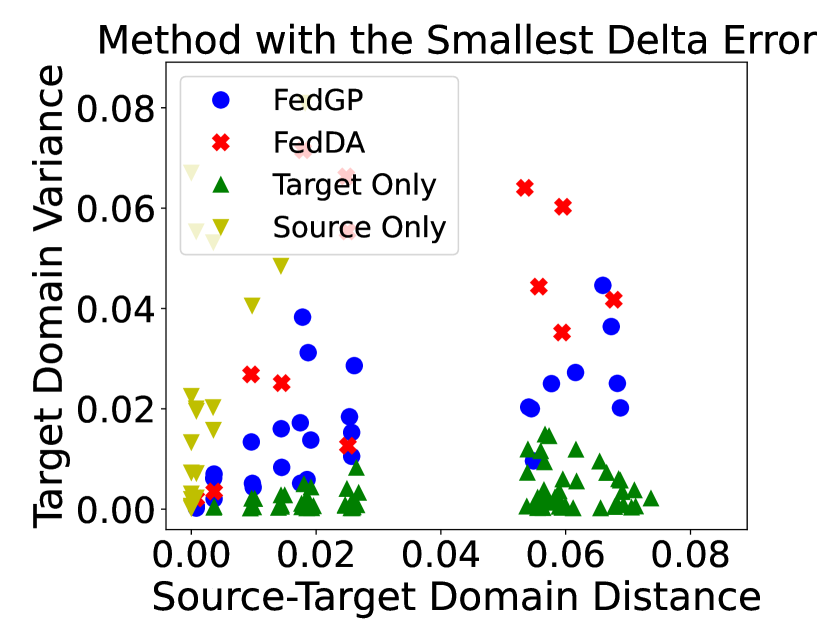
(a)

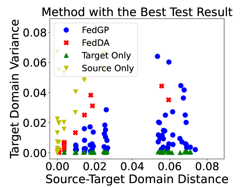
(b)

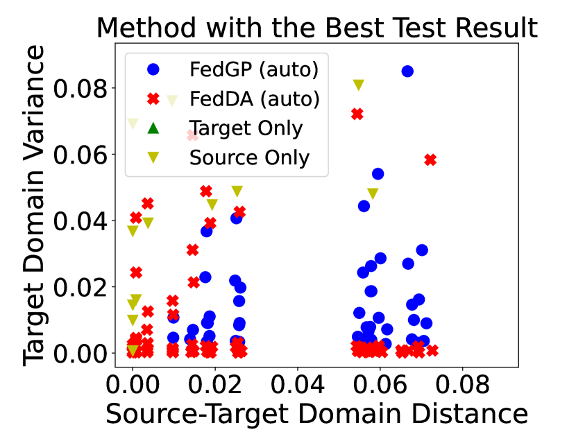
(c)

Figure 2: Given specific source-target domain distance and target domain variance: (a) shows which aggregation method has the smallest Delta error; (b)&(c) present which aggregation method actually achieves the best test result. In (a)&(b), FedDA and FedGP use a fixed $\beta=0.5$. In (c), FedDA and FedGP adopt the auto-weighted scheme. Observations: Comparing (a) and (b), we can see that the prediction from the Delta errors, computed at initialization, mostly track the actual test performance after training. Comparing (b) and (c), we can see that FedDA is greatly improved with the auto-weighted scheme. Moreover, we can see that FedGP with a fixed $\beta=0.5$ is good enough for most of the cases. These observations demonstrate the practical utility of our theoretical framework.

The synthetic data experiment aims to bridge the gap between theory and practice by verifying our theoretical insights. Specifically, we generate various source and target datasets and compute the corresponding source-target domain distance $d_{\pi}({\mathcal{D}}_{S},{\mathcal{D}}_{T})$ and target domain variance $\sigma_{\pi}(\widehat{\mathcal{D}}_{T})$. We aim to verify if our theory is predictive of practice.

In this experiment, we use one-hidden-layer neural networks with sigmoid activation. We generate $9$ datasets $D_{1},\dots,D_{9}$ each consisting of 5000 data points as the following. We first generate 5000 samples $x\in{\mathbb{R}}^{50}$ from a mixture of $10$ Gaussians. The ground truth target is set to be the sum of $100$ radial basis functions, the target has $10$ samples. We control the randomness and deviation of the basis function to generate datasets with domain shift. As a result, $D_{2}$ to $D_{9}$ have an increasing domain-shift compared to $D_{1}$. We take $D_{1}$ as the target domain. We subsample (uniformly) 9 datasets $\widehat{D}^{1}_{1},\dots,\widehat{D}^{9}_{1}$ from $D_{1}$ with decreasing number of subsamples. As a result, $\widehat{D}^{1}_{1}$ has the smallest target domain variance, and $\widehat{D}^{9}_{1}$ has the largest. Additional details about the datasets are deferred to Appendix B.

Methods. For each pair of $(D_{i},\widehat{D}_{1}^{j})$ where $i,j=1,\dots,9$ from the 81 pairs of datasets. We compute the source-target domain distance $d_{\pi}(D_{i},\widehat{D}_{1}^{j})$ and target domain variance $\sigma_{\pi}(\widehat{D}_{1}^{j})$ with $\pi$ being the point mass on only the initialization parameter. We then train the 2-layer neural network with different aggregation strategies on $(D_{i},\widehat{D}_{1}^{j})$. Given the pair of datasets, we identify which strategies has the smallest Delta error and the best test performance on the target domain.

As interpreted in Figure 2, the results verify that (i) the Delta error indicates the actual test result, and (ii) the auto-weighted strategy, which minimizes the estimated Delta error, is effective in practice.

6 Experimental Evaluations

In this section, we present and discuss the results of various dataset experiments. The algorithm outline, technical implementation details of the auto-weighted and gradient projection aggregation, as well as extended experiments can be found in Appendix C.1 &  C.3 &  C.8. More ablation study and visualization results are available in Appendix C.4 &  C.7.

6.1 Real Dataset Experiments

	ColoredMNIST				VLCS					TerraIncognita
Domains	+90%	+80%	-90%	Avg	C	L	V	S	Avg	Avg
Source Only	56.82	62.37	27.77	48.99	90.49	60.65	70.24	69.10	72.62	37.50
Finetune_Offline	66.58	69.09	53.86	63.18	96.65	68.22	74.34	74.66	78.47	68.18
FedDA	60.49	65.07	33.04	52.87	97.72	68.17	75.27	76.68	79.46	64.70
FedGP	88.14	76.34	89.80	84.76	99.43	71.09	73.65	78.70	80.72	71.24
FedDA_Auto	87.41	76.33	85.57	83.10	99.41	70.99	75.38	80.08	81.46	71.76
FedGP_Auto	89.85	76.43	89.62	85.30	99.48	70.71	75.24	79.99	81.36	71.58
Target Only	85.60	73.54	87.05	82.06	97.77	68.88	72.29	76.00	78.74	67.24
FedAvg	63.17	71.92	10.92	48.67	96.31	68.03	69.84	68.67	75.71	30.00
Ditto [18]	62.17	71.26	19.32	50.92	95.94	67.45	70.48	66.05	74.98	28.75
FedRep [4]	65.41	36.44	31.72	44.52	91.14	60.39	70.31	70.06	72.98	20.86
APFL [6]	43.78	61.60	30.23	45.20	68.63	60.98	65.40	49.85	61.22	52.72
KNN-per [21]	64.87	71.24	10.44	48.85	96.31	68.04	69.84	68.67	75.72	30.00
Oracle	89.94	80.32	89.99	86.75	100.00	72.72	78.65	82.71	83.52	93.11

Table 1: Target domain test accuracy (%) on ColoredMNIST, VLCS, and TerraIncognita. The results reveal that our auto-weighted methods consistently deliver superior performance in most cases, and some of their accuracies approach the corresponding ground-truth upper bound (Oracle). The auto-weighted scheme improves FedDA significantly. Interestingly, we observe that FedGP, even with default fixed betas ($\beta=0.5$), is capable of achieving competitive results. Furthermore, when compared to standard personalized FL benchmarks, our methods surpass them by significant margins, demonstrating the effectiveness of our approach. Full TerraIncognita results are in Appendix C.2.

Datasets, models, and baselines. We use the Domainbed [9] benchmark with multiple domains, with realistic shifts between source and target clients. We conduct experiments on three datasets: ColoredMNIST [1], VLCS [7], and TerraIncognita [2] datasets. We use $0.1\%$ samples of ColoredMNIST, $5\%$ samples of VLCS, and $5\%$ of TerraIncognita for their respective target domains. The task is doing classification of the target domain. We use a CNN model for ColoredMNIST and ResNet-18 [11] for the other two datasets. For baselines in particular, we compare Finetune_Offline (fine-tuning locally after source-only training), auto-weighted methods FedDA_Auto and FedGP_Auto, the Oracle (supervised training with all target data (${\mathcal{D}}_{T}$)), FedAvg, as well as personalization baselines Ditto [18], FedRep [4], APFL [6], and KNN-per [21].

Implementation. We set the total round $R=50$ and the local update epoch to $1$. For each dataset, we test the target performance of individual domains using the left-out domain as the target and the rest as source domains. The accuracies averaged over 5 trials are reported. We report and discuss in Table 1 the FDA performance (test accuracy on the target domain) of each method. More implementation details can be found in Appendix C.2.

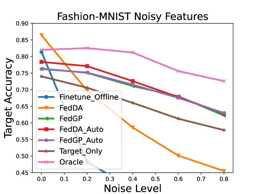
(a) Fashion-MNIST noisy features

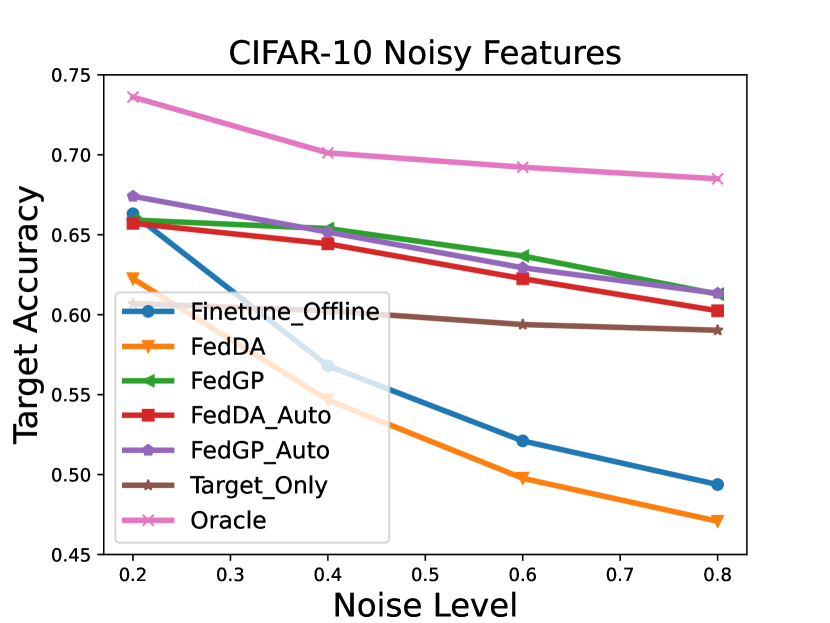
(b) CIFAR-10 noisy features

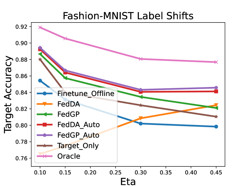
(c) Fashion-MNIST label shifts

Figure 3: The impact of changing domain shifts with noisy features or label shifts. We observe that the auto-weighted methods and even FedGP with a fixed weight ($\beta=0.5$) show good abilities to balance bias and variances and are less sensitive to domain shifts.

6.2 Ablation Study and Discussion

The effect of varying source-target domain shifts.

We empirically investigate the sensitivity of each method to domain shifts in semi-synthetic experiments. We adjust the extent of domain shifts by introducing varying levels of Gaussian noise (noisy features) and degrees of class imbalance (label shifts). The results are shown and discussed in Figure 3. Full results can be found in Appendix C.6.

The effect of source-target balancing weight $\beta$.

We conduct experiment on FedDA and FedGP with varying $\beta$ on Fashion-MNIST, CIFAR10, and Colored-MNIST. The results are shown and discussed in Figure 4. Additionally, complete results are in Appendix C.5.

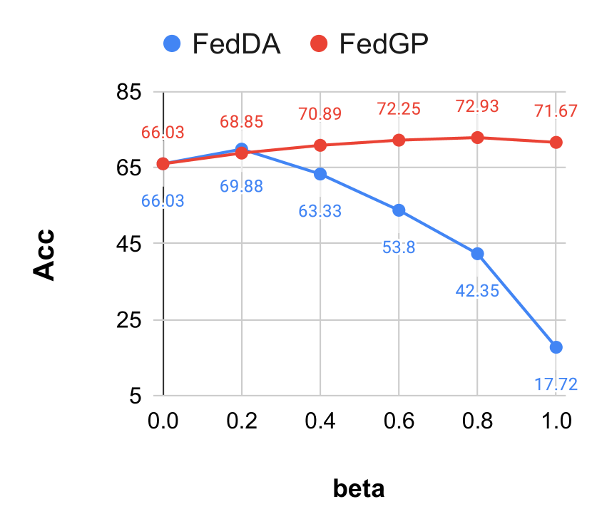
(a) Fashion-MNIST (0.4 noise level)

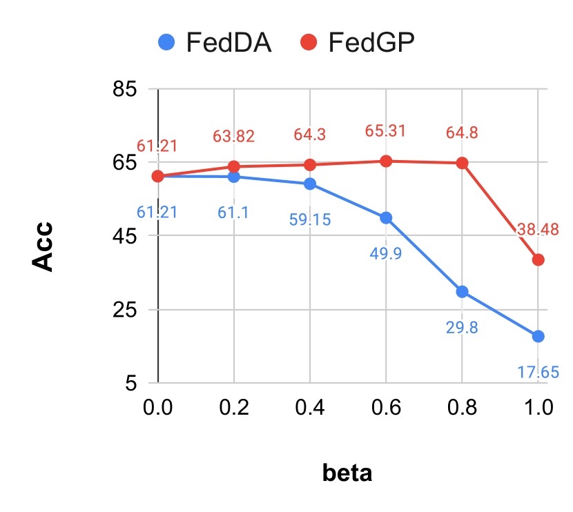
(b) CIFAR-10 (0.4 noise level)

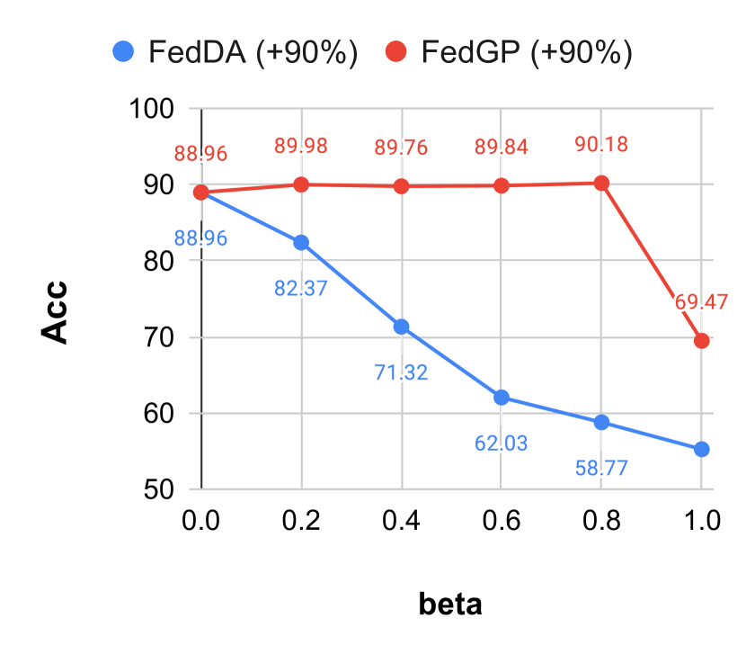
(c) ColoredMNIST (target: +90%)

Figure 4: The effect of $\beta$ on FedDA and FedGP on Fashion-MNIST, CIFAR10, and Colored-MNIST. In most cases, we observe FedGP outperforming FedDA, and FedDA being more sensitive to the varying $\beta$ values. This suggests that the auto-weighted FedDA is able to choose optimal enough $\beta$.

Effectiveness of projection and filtering. In Table 2, we illustrate the effectiveness of using gradient projection and filtering in Fashion-MNIST and CIFAR-10 noisy feature experiments. Compared with FedDA which does not perform gradient projection, FedGP manages to achieve a large margin ($\sim 15\%$) of performance gain, especially when the shifts are larger. Further, with filtering, we generally get a $1\%\sim 2\%$ performance gain compared with no filtering.

	Fashion-MNIST				CIFAR-10
Target noise level	0.2	0.4	0.6	0.8	0.2	0.4	0.6	0.8
FedDA(w/o projection)	69.73	58.60	50.13	45.51	62.25	54.67	49.77	47.08
FedGP(w/o filter)	72.93	69.51	65.46	60.70	66.51	64.04	62.06	60.91
FedGP(w filter)	75.09	71.09	68.01	62.22	66.40	65.28	63.29	61.59

Table 2: Effectiveness of the gradient projection and filtering operations.

Discussion. The analysis of the computational and communication cost for our proposed aggregation methods are discussed in Appendix C.9&  C.3, where we show how the proposed aggregation rules, especially the auto-weighted operation, can be done efficiently. Moreover, we observe in our experiments that Finetune_Offline is vastly sensitive to its pre-trained model (which is obtained via FedAvg), highlighting the necessity of a deeper study on the relations between personalization and domain adaptation. Lastly, we note that our current setting considers supervised tasks with limited target data samples. Although different from the unsupervised FDA [24, 19, 8, 28] and semi-supervised domain adaptation [25, 14] settings, we conduct experiments comparing them as shown in Appendix C.10 and  C.11. We observe that our auto-weighted methods have better or comparable performance across domains, especially for large shift cases. However, we acknowledge the possibility of extending the current framework to a semi-supervised setting, which serves as an interesting future work.

7 Conclusion

In this work, we provide a theoretical framework that first formally defines the metrics to connect FDA settings with aggregation rules. We propose FedGP, a filtering-based aggregation rule via gradient projection, and develop the auto-weighted scheme that dynamically finds the best weights - both significantly improve the target performances. For future work, we plan to extend the current framework to perform FDA simultaneously on several source/target clients, explore the relationship between personalization and adaptation, as well as devise stronger aggregation rules for the FDA problem.

Federated Auto-weighted Domain Adaptation
Appendix

Appendix Contents

• Section A: Supplementary Theoretical Results

  • A.1: Proofs

    • A.1.1: Proof of Theorem 3.2

    • A.1.2: Proof of Theorem 4.2

    • A.1.3: Proof of Theorem 4.4

  • A.2: Additional Discussion of the Auto-weighting Method

• Section B: Synthetic Data Experiments in Details

• Section C: Supplementary Experiment Information

  • C.1: Algorithm Outlines for Federated Domain Adaptation

  • C.2: Real-World Experiment Implementation Details and Results

  • C.3: Auto-Weighted Methods: Implementation Details, Time and Space Complexity

  • C.4: Visualization of Auto-Weighted Betas Values on Real-World Datasets

  • C.5: Additional Experiment Results on Varying Static Weights ($\beta$)

  • C.6: Semi-Synthetic Experiment Settings, Implementation, and Results

  • C.7: Additional Ablation Study Results

  • C.8: Implementation Details of FedGP

  • C.9: Gradient Projection Method’s Time and Space Complexity

  • C.10: Comparison with the Unsupervised FDA Method

  • C.11: Comparison with the Semi-Supervised Domain Adaptation (SSDA) Method

Appendix A Supplementary Theoretical Results

In this section, we provide theoretical results that are omitted in the main paper due to space limitation. Specifically, in subsection A.1 we provide proofs to our theorems. Further, in subsection A.2 we present omitted discussion for our auto-weighting method, including how the estimators are constructed.

A.1 Proofs

A.1.1 Proof of Theorem 3.2

We prove Theorem 3.2 by proving a generalized version of it, as shown below as Theorem A.1. Note that Theorem A.1 reduce to Theorem 3.2 when the step size $\mu=\tfrac{1}{\gamma}$, corresponding to the fastest loss value descent.

Theorem A.1 (Theorem 3.2 Generalized).

Consider model parameter $\theta\sim\pi$ and an aggregation rule Aggr$(\cdot)$ with step size $\mu>0$. Define the updated parameter as

$$\theta^{+}:=\theta-\mu\widehat{g}_{\texttt{Aggr}}(\theta).$$ (14)

Assuming the gradient $\nabla\ell(\theta,z)$ is $\gamma$-Lipschitz in $\theta$ for any $z$, and let the step size $\mu\leq\tfrac{1}{\gamma},$ we have

$$\mathbb{E}_{\widehat{\mathcal{D}}_{T},\theta}[\ell_{{\mathcal{D}}_{T}}(\theta^{+})-\ell_{{\mathcal{D}}_{T}}(\theta)]\leq-\tfrac{\mu}{2}(\|g_{{\mathcal{D}}_{T}}\|_{\pi}^{2}-\Delta^{2}_{\texttt{Aggr}}).$$ (15)

Proof.

Given any distribution data ${\mathcal{D}}$, we first prove that $\nabla\ell_{\mathcal{D}}$ is also $\gamma$-Lipschitz as below. For $\forall\theta_{1},\theta_{2}\in\Theta$:

$$\|\nabla\ell_{\mathcal{D}}(\theta_{1})-\nabla\ell_{{\mathcal{D}}}(\theta_{2})\| =\|\mathbb{E}_{z\sim{\mathcal{D}}}[\nabla\ell(\theta_{1},z)-\nabla\ell(\theta_{2},z)]\|$$ (16)

$$\leq\mathbb{E}_{z\sim{\mathcal{D}}}\|\nabla\ell(\theta_{1},z)-\nabla\ell(\theta_{2},z)\|$$ (Jensen’s inequality)

$$\leq\mathbb{E}_{z\sim{\mathcal{D}}}\gamma\|\theta_{1}-\theta_{2}\| \nabla\ell(\cdot,z) \gamma$$ ( is -Lipschitz)

$$=\gamma\|\theta_{1}-\theta_{2}\|.$$ (17)

Therefore, we know that $\ell_{{\mathcal{D}}_{T}}$ is $\gamma$-smooth. Conditioned on a $\theta$ and a $\widehat{\mathcal{D}}_{T}$, and apply the definition of smoothness we have

$$\ell_{{\mathcal{D}}_{T}}( \theta^{+})-\ell_{{\mathcal{D}}_{T}}(\theta)\leq\langle\nabla\ell_{{\mathcal{D}}_{T}}(\theta),\theta^{+}-\theta\rangle+\frac{\gamma}{2}\|\theta^{+}-\theta\|^{2}$$ (18)

$$=-\langle\nabla\ell_{{\mathcal{D}}_{T}}(\theta),\mu\widehat{g}_{\texttt{Aggr}}(\theta)\rangle+\frac{\gamma}{2}\|\mu\widehat{g}_{\texttt{Aggr}}(\theta)\|^{2}$$ (19)

$$=-\mu\langle\nabla\ell_{{\mathcal{D}}_{T}}(\theta),\widehat{g}_{\texttt{Aggr}}(\theta)-\nabla\ell_{{\mathcal{D}}_{T}}(\theta)+\nabla\ell_{{\mathcal{D}}_{T}}(\theta)\rangle$$ (20)

$$\qquad+\frac{\gamma\mu^{2}}{2}\|\widehat{g}_{\texttt{Aggr}}(\theta)-\nabla\ell_{{\mathcal{D}}_{T}}(\theta)+\nabla\ell_{{\mathcal{D}}_{T}}(\theta)\|^{2}$$ (21)

$$=-\mu(\langle\nabla\ell_{{\mathcal{D}}_{T}}(\theta),\widehat{g}_{\texttt{Aggr}}(\theta)-\nabla\ell_{{\mathcal{D}}_{T}}(\theta)\rangle+\|\nabla\ell_{{\mathcal{D}}_{T}}(\theta)\|^{2})$$ (22)

$$\qquad+\frac{\gamma\mu^{2}}{2}(\|\widehat{g}_{\texttt{Aggr}}(\theta)-\nabla\ell_{{\mathcal{D}}_{T}}(\theta)\|^{2}+\|\nabla\ell_{{\mathcal{D}}_{T}}(\theta)\|^{2}+2\langle\widehat{g}_{\texttt{Aggr}}(\theta)-\nabla\ell_{{\mathcal{D}}_{T}}(\theta),\nabla\ell_{{\mathcal{D}}_{T}}(\theta)\rangle)$$ (23)

$$=(\mu-\gamma\mu^{2})(\langle\nabla\ell_{{\mathcal{D}}_{T}}(\theta),\nabla\ell_{{\mathcal{D}}_{T}}(\theta)-\widehat{g}_{\texttt{Aggr}}(\theta)\rangle)$$ (24)

$$\qquad+(\frac{\gamma\mu^{2}}{2}-\mu)\|\nabla\ell_{{\mathcal{D}}_{T}}(\theta)\|^{2}+\frac{\gamma\mu^{2}}{2}\|\widehat{g}_{\texttt{Aggr}}(\theta)-\nabla\ell_{{\mathcal{D}}_{T}}(\theta)\|^{2}$$ (25)

$$\leq(\mu-\gamma\mu^{2})\cdot\|\nabla\ell_{{\mathcal{D}}_{T}}(\theta)\|\cdot\|\widehat{g}_{\texttt{Aggr}}(\theta)-\nabla\ell_{{\mathcal{D}}_{T}}(\theta)\|$$ (Cauchy–Schwarz inequality)

$$\qquad+(\frac{\gamma\mu^{2}}{2}-\mu)\|\nabla\ell_{{\mathcal{D}}_{T}}(\theta)\|^{2}+\frac{\gamma\mu^{2}}{2}\|\widehat{g}_{\texttt{Aggr}}(\theta)-\nabla\ell_{{\mathcal{D}}_{T}}(\theta)\|^{2}.$$ (26)

$$\leq\frac{\mu-\gamma\mu^{2}}{2}\left(\|\nabla\ell_{{\mathcal{D}}_{T}}(\theta)\|^{2}+\|\widehat{g}_{\texttt{Aggr}}(\theta)-\nabla\ell_{{\mathcal{D}}_{T}}(\theta)\|^{2}\right)$$ (AM-GM inequality)

$$\qquad+(\frac{\gamma\mu^{2}}{2}-\mu)\|\nabla\ell_{{\mathcal{D}}_{T}}(\theta)\|^{2}+\frac{\gamma\mu^{2}}{2}\|\widehat{g}_{\texttt{Aggr}}(\theta)-\nabla\ell_{{\mathcal{D}}_{T}}(\theta)\|^{2}.$$ (27)

$$=-\frac{\mu}{2}\left(\|\nabla\ell_{{\mathcal{D}}_{T}}(\theta)\|^{2}-\|\widehat{g}_{\texttt{Aggr}}(\theta)-\nabla\ell_{{\mathcal{D}}_{T}}(\theta)\|^{2}\right).$$ (28)

Additionally, note that the above two inequalities stand because: the step size $\mu\leq\frac{1}{\gamma}$ and thus $\mu-\gamma\mu^{2}=\mu^{2}(\tfrac{1}{\mu}-\gamma)\geq 0$. Taking the expectation $\mathbb{E}_{\widehat{\mathcal{D}}_{T},\theta}$ on both sides gives

$$\mathbb{E}_{\widehat{\mathcal{D}}_{T},\theta}[\ell_{{\mathcal{D}}_{T}}(\theta^{+})-\ell_{{\mathcal{D}}_{T}}(\theta)]\leq-\frac{\mu}{2}\left(\mathbb{E}_{\widehat{\mathcal{D}}_{T},\theta}[\|\nabla\ell_{{\mathcal{D}}_{T}}(\theta)\|^{2}]-\mathbb{E}_{\widehat{\mathcal{D}}_{T},\theta}[\|\widehat{g}_{\texttt{Aggr}}(\theta)-\nabla\ell_{{\mathcal{D}}_{T}}(\theta)\|^{2}]\right)$$ (29)

Note that we denote $g_{{\mathcal{D}}_{T}}=\nabla\ell_{{\mathcal{D}}_{T}}$. Thus, with the $L^{\pi}$ norm notation we have

$$\mathbb{E}_{\widehat{\mathcal{D}}_{T},\theta}[\ell_{{\mathcal{D}}_{T}}(\theta^{+})-\ell_{{\mathcal{D}}_{T}}(\theta)]\leq-\frac{\mu}{2}\left(\|g_{{\mathcal{D}}_{T}}\|_{\pi}^{2}-\mathbb{E}_{\widehat{\mathcal{D}}_{T}}\|\widehat{g}_{\texttt{Aggr}}-g_{{\mathcal{D}}_{T}}\|_{\pi}^{2}\right).$$ (30)

Finally, by Definition 3.1 we can see $\Delta^{2}_{\texttt{Aggr}}=\mathbb{E}_{\widehat{\mathcal{D}}_{T}}\|\widehat{g}_{\texttt{Aggr}}-g_{{\mathcal{D}}_{T}}\|_{\pi}^{2}$, which concludes the proof. ∎

A.1.2 Proof of Theorem 4.2

Next, we prove the following theorem.

Theorem A.2 (Theorem 4.2 Restated).

Consider FedDA. Given the target domain $\widehat{\mathcal{D}}_{T}$ and $N$ source domains ${\mathcal{D}}_{S_{1}},\dots,{\mathcal{D}}_{S_{N}}$.

$$\Delta^{2}_{\texttt{FedDA}}\leq\sum_{i=1}^{N}\alpha_{i}\Delta^{2}_{\texttt{FedDA},S_{i}},\quad\text{where }\ \Delta^{2}_{\texttt{FedDA},S_{i}}=(1-\beta_{i})^{2}\sigma_{\pi}^{2}(\widehat{\mathcal{D}}_{T})+\beta_{i}^{2}d^{2}_{\pi}({\mathcal{D}}_{S_{i}},{\mathcal{D}}_{T})$$ (31)

is the Delta error when only considering ${\mathcal{D}}_{S_{i}}$ as the source domain.

Proof.

Recall

$$\widehat{g}_{\texttt{FedDA}} =\sum_{i=1}^{N}\alpha_{i}\left((1-\beta_{i})g_{\widehat{\mathcal{D}}_{T}}+\beta_{i}g_{{\mathcal{D}}_{S_{i}}}\right).$$ (32)

Thus, noting that $\sum_{i}\alpha_{i}=1$ as defined in Definition 4.1,

$$\Delta^{2}_{\texttt{FedDA}} =\mathbb{E}_{\widehat{\mathcal{D}}_{T}}\|g_{{\mathcal{D}}_{T}}-\widehat{g}_{\texttt{FedDA}}\|^{2}_{\pi}=\mathbb{E}_{\widehat{\mathcal{D}}_{T}}\big{\|}g_{{\mathcal{D}}_{T}}-\sum_{i=1}^{N}\alpha_{i}\left((1-\beta_{i})g_{\widehat{\mathcal{D}}_{T}}+\beta_{i}g_{{\mathcal{D}}_{S_{i}}}\right)\big{\|}^{2}_{\pi}$$ (33)

$$=\mathbb{E}_{\widehat{\mathcal{D}}_{T}}\big{\|}\sum_{i=1}^{N}\alpha_{i}\left(g_{{\mathcal{D}}_{T}}-(1-\beta_{i})g_{\widehat{\mathcal{D}}_{T}}+\beta_{i}g_{{\mathcal{D}}_{S_{i}}}\right)\big{\|}^{2}_{\pi}$$ (34)

$$\leq\sum_{i=1}^{N}\alpha_{i}\mathbb{E}_{\widehat{\mathcal{D}}_{T}}\big{\|}g_{{\mathcal{D}}_{T}}-(1-\beta_{i})g_{\widehat{\mathcal{D}}_{T}}+\beta_{i}g_{{\mathcal{D}}_{S_{i}}}\big{\|}^{2}_{\pi}$$ (35)

where the inequality is derived by Jensen’s inequality. Next, we prove for each $i\in[N]$:

$$\mathbb{E}_{\widehat{\mathcal{D}}_{T}} \big{\|}g_{{\mathcal{D}}_{T}}-(1-\beta_{i})g_{\widehat{\mathcal{D}}_{T}}+\beta_{i}g_{{\mathcal{D}}_{S_{i}}}\big{\|}^{2}_{\pi}=\mathbb{E}_{\widehat{\mathcal{D}}_{T}}\|(1-\beta_{i})(g_{{\mathcal{D}}_{T}}-g_{\widehat{\mathcal{D}}_{T}})+\beta_{i}(g_{{\mathcal{D}}_{T}}-g_{{\mathcal{D}}_{S_{i}}})\|^{2}_{\pi}$$ (36)

$$=(1-\beta_{i})^{2}\mathbb{E}_{\widehat{\mathcal{D}}_{T}}\|g_{{\mathcal{D}}_{T}}-g_{\widehat{\mathcal{D}}_{T}}\|_{\pi}^{2}+\beta_{i}^{2}\|g_{{\mathcal{D}}_{T}}-g_{{\mathcal{D}}_{S_{i}}}\|^{2}_{\pi}$$ (37)

$$\qquad\qquad+2(1-\beta_{i})\beta_{i}\mathbb{E}_{\widehat{\mathcal{D}}_{T}}\langle g_{{\mathcal{D}}_{T}}-g_{\widehat{\mathcal{D}}_{T}},g_{{\mathcal{D}}_{T}}-g_{{\mathcal{D}}_{S_{i}}}\rangle_{\pi}$$ (38)

$$=(1-\beta_{i})^{2}\sigma_{\pi}^{2}(\widehat{\mathcal{D}}_{T})+\beta_{i}^{2}d^{2}_{\pi}({\mathcal{D}}_{S},{\mathcal{D}}_{T})+2(1-\beta_{i})\beta_{i}\langle\mathbb{E}_{\widehat{\mathcal{D}}_{T}}[g_{{\mathcal{D}}_{T}}-g_{\widehat{\mathcal{D}}_{T}}],g_{{\mathcal{D}}_{T}}-g_{{\mathcal{D}}_{S_{i}}}\rangle_{\pi}$$ (39)

$$=(1-\beta_{i})^{2}\sigma_{\pi}^{2}(\widehat{\mathcal{D}}_{T})+\beta_{i}^{2}d^{2}_{\pi}({\mathcal{D}}_{S_{i}},{\mathcal{D}}_{T})$$ (40)

$$=\Delta^{2}_{\texttt{FedDA},S_{i}}.$$ (41)

Plugging the above equation into (35) gives the theorem. ∎

A.1.3 Proof of Theorem 4.4

Theorem 4.4, rigorously speaking, is the result of the following theorem and a set of approximations. We first present the following theorem which gives an upper bound for $\Delta^{2}_{\texttt{FedGP}}$ rigorously. Then, we show how we approximate the result into what Theorem 4.4 states, which is also what we actually use for FedGP’s auto-weighted version.

Theorem A.3 (Formal Version of Theorem 4.4).

Consider FedGP. Given the target domain $\widehat{\mathcal{D}}_{T}$ and $N$ source domains ${\mathcal{D}}_{S_{1}},\dots,{\mathcal{D}}_{S_{N}}$.

$$\Delta^{2}_{\texttt{FedGP}} \leq\sum_{i=1}^{N}\alpha_{i}\Delta^{2}_{\texttt{FedGP},S_{i}},$$ (42)

where

$$\Delta^{2}_{\texttt{FedGP},S_{i}} =(1-\beta_{i})^{2}\sigma_{\pi}^{2}(\widehat{\mathcal{D}}_{T})+\beta_{i}^{2}\mathbb{E}_{\theta,\widehat{\mathcal{D}}_{T}}[\widehat{\delta}_{i}(\theta)\tau_{i}^{2}(\theta)\|g_{{\mathcal{D}}_{T}}(\theta)-g_{{\mathcal{D}}_{S_{i}}}(\theta)\|^{2}]$$ (43)

$$\ +(2\beta_{i}-\beta_{i}^{2})\mathbb{E}_{\theta,\widehat{\mathcal{D}}_{T}}\widehat{\delta}_{i}(\theta)\langle g_{\widehat{\mathcal{D}}_{T}}(\theta)-g_{{\mathcal{D}}_{T}}(\theta),u_{{\mathcal{D}}_{S_{i}}}(\theta)\rangle^{2}$$ (44)

$$\ +2\beta_{i}(1-\beta_{i})\mathbb{E}_{\theta,\widehat{\mathcal{D}}_{T}}[\widehat{\delta}_{i}(\theta)\langle g_{{\mathcal{D}}_{T}}(\theta),g_{{\mathcal{D}}_{S_{i}}}(\theta)\rangle\cdot\langle g_{\widehat{\mathcal{D}}_{T}}(\theta)-g_{{\mathcal{D}}_{T}}(\theta),u_{{\mathcal{D}}_{S_{i}}}(\theta)\rangle]$$ (45)

$$\qquad+\beta_{i}^{2}\mathbb{E}_{\theta,\widehat{\mathcal{D}}_{T}}[(1-\widehat{\delta}_{i}(\theta))\|g_{{\mathcal{D}}_{T}}(\theta)\|^{2}].$$ (46)

In the above equation, $\widehat{\delta}_{i}(\theta):=\bm{1}(\langle g_{\widehat{\mathcal{D}}_{T}}(\theta),g_{{\mathcal{D}}_{S_{i}}}(\theta)\rangle>0)$ is the indicator function and it is $1$ if the condition is satisfied. $\tau_{i}(\theta):=\tfrac{\|g_{{\mathcal{D}}_{T}}(\theta)\sin\rho_{i}(\theta)\|}{\|g_{{\mathcal{D}}_{S_{i}}}(\theta)-g_{{\mathcal{D}}_{T}}(\theta)\|}$ where $\rho_{i}(\theta)$ is the angle between $g_{{\mathcal{D}}_{S_{i}}}(\theta)$ and $g_{{\mathcal{D}}_{T}}(\theta)$. Moreover, $u_{{\mathcal{D}}_{S_{i}}}(\theta):=g_{{\mathcal{D}}_{S_{i}}}(\theta)/\|g_{{\mathcal{D}}_{S_{i}}}(\theta)\|$.

Proof.

Recall that

$$\widehat{g}_{\texttt{FedGP}}(\theta)=\sum_{i=1}^{N}\alpha_{i}\left((1-\beta_{i})g_{\widehat{\mathcal{D}}_{T}}(\theta)+\beta_{i}\texttt{Proj}_{+}(g_{\widehat{\mathcal{D}}_{T}}(\theta)|g_{{\mathcal{D}}_{S_{i}}}(\theta))\right)=\sum_{i=1}^{N}\alpha_{i}\widehat{g}_{\texttt{FedGP},{\mathcal{D}}_{S_{i}}}(\theta),$$ (47)

where we denote

$$\widehat{g}_{\texttt{FedGP},{\mathcal{D}}_{S_{i}}}(\theta)\coloneqq\left((1-\beta_{i})g_{\widehat{\mathcal{D}}_{T}}(\theta)+\beta_{i}\texttt{Proj}_{+}(g_{\widehat{\mathcal{D}}_{T}}(\theta)|g_{{\mathcal{D}}_{S_{i}}}(\theta))\right).$$ (48)

From the definition of $\Delta^{2}_{\texttt{FedGP}}$, noting that $\sum_{i}\alpha_{i}=1$ as defined in Definition 4.3, and we can derive:

$$\Delta^{2}_{\texttt{FedGP}} =\mathbb{E}_{\widehat{\mathcal{D}}_{T}}\|g_{{\mathcal{D}}_{T}}-\widehat{g}_{\texttt{FedGP}}\|^{2}_{\pi}=\mathbb{E}_{\widehat{\mathcal{D}}_{T},\theta}\|g_{{\mathcal{D}}_{T}}(\theta)-\widehat{g}_{\texttt{FedGP}}(\theta)\|^{2}$$ (49)

$$=\mathbb{E}_{\widehat{\mathcal{D}}_{T},\theta}\|g_{{\mathcal{D}}_{T}}(\theta)-\sum_{i=1}^{N}\alpha_{i}\widehat{g}_{\texttt{FedGP},{\mathcal{D}}_{S_{i}}}(\theta)\|^{2}$$ (50)

$$=\mathbb{E}_{\widehat{\mathcal{D}}_{T},\theta}\|\sum_{i=1}^{N}\alpha_{i}(g_{{\mathcal{D}}_{T}}(\theta)-\widehat{g}_{\texttt{FedGP},{\mathcal{D}}_{S_{i}}}(\theta))\|^{2}$$ (51)

$$\leq\sum_{i=1}^{N}\alpha_{i}\mathbb{E}_{\widehat{\mathcal{D}}_{T},\theta}\|g_{{\mathcal{D}}_{T}}(\theta)-\widehat{g}_{\texttt{FedGP},{\mathcal{D}}_{S_{i}}}(\theta)\|^{2}$$ (52)

where the inequality is derived by Jensen’s inequality.

Next, we show $\mathbb{E}_{\widehat{\mathcal{D}}_{T},\theta}\|g_{{\mathcal{D}}_{T}}(\theta)-\widehat{g}_{\texttt{FedGP},{\mathcal{D}}_{S_{i}}}(\theta)\|^{2}=\Delta^{2}_{\texttt{FedGP},S_{i}}$. First, we simplify the notation. Recall the definition of $\widehat{g}_{\texttt{FedGP},{\mathcal{D}}_{S_{i}}}$ is that

$$\widehat{g}_{\texttt{FedGP},{\mathcal{D}}_{S_{i}}}(\theta) =(1-\beta_{i})g_{\widehat{\mathcal{D}}_{T}}(\theta)+\beta_{i}\max\{\langle g_{\widehat{\mathcal{D}}_{T}}(\theta),g_{{\mathcal{D}}_{S_{i}}}\rangle,0\}g_{{\mathcal{D}}_{S_{i}}(\theta)}/\|g_{{\mathcal{D}}_{S_{i}}}(\theta)\|^{2}$$ (53)

$$=(1-\beta_{i})g_{\widehat{\mathcal{D}}_{T}}(\theta)+\beta_{i}\widehat{\delta}_{i}(\theta)\langle g_{\widehat{\mathcal{D}}_{T}}(\theta),u_{{\mathcal{D}}_{S_{i}}}(\theta)\rangle u_{{\mathcal{D}}_{S_{i}}}(\theta).$$ (54)

Let us fix $\theta$ and then further simplify the notation by denoting

$$\hat{v} :=g_{\widehat{\mathcal{D}}_{T}}(\theta)$$ (55)

$$v :=g_{{\mathcal{D}}_{T}}(\theta)$$ (56)

$$u :=u_{{\mathcal{D}}_{S_{i}}}(\theta)$$ (57)

$$\hat{\delta} :=\hat{\delta}_{i}(\theta)$$ (58)

Therefore, we have $\widehat{g}_{\texttt{FedGP},{\mathcal{D}}_{S_{i}}}(\theta)=(1-\beta_{i})\hat{v}+\beta_{i}\hat{\delta}\langle\hat{v},u\rangle u$.

Therefore, with the simplified notation,

$$\mathbb{E}_{\widehat{\mathcal{D}}_{T}}\|g_{{\mathcal{D}}_{T}} (\theta)-\widehat{g}_{\texttt{FedGP},{\mathcal{D}}_{S_{i}}}(\theta)\|^{2}=\mathbb{E}_{\widehat{\mathcal{D}}_{T}}\|(1-\beta_{i})\hat{v}+\beta_{i}\hat{\delta}\langle\hat{v},u\rangle u-v\|^{2}$$ (59)

$$=\mathbb{E}_{\widehat{\mathcal{D}}_{T}}\|\beta_{i}(\hat{\delta}\langle\hat{v},u\rangle u-v)+(1-\beta_{i})(\hat{v}-v)\|^{2}$$ (60)

$$=\mathbb{E}_{\widehat{\mathcal{D}}_{T}}\|\beta_{i}\hat{\delta}\langle\hat{v}-v,u\rangle u+\beta_{i}(\hat{\delta}\langle v,u\rangle u-v)+(1-\beta_{i})(\hat{v}-v)\|^{2}$$ (61)

$$=\beta_{i}^{2}\mathbb{E}_{\widehat{\mathcal{D}}_{T}}[\hat{\delta}\langle\hat{v}-v,u\rangle^{2}]+\beta_{i}^{2}\mathbb{E}_{\widehat{\mathcal{D}}_{T}}[\|\hat{\delta}\langle v,u\rangle u-v\|^{2}]+(1-\beta_{i})^{2}\mathbb{E}_{\widehat{\mathcal{D}}_{T}}[\|\hat{v}-v\|^{2}]$$ (62)

$$\qquad+2\beta_{i}(1-\beta_{i})\mathbb{E}_{\widehat{\mathcal{D}}_{T}}[\hat{\delta}\langle\hat{v}-v,u\rangle^{2}]+2\beta_{i}(1-\beta_{i})\mathbb{E}_{\widehat{\mathcal{D}}_{T}}[\hat{\delta}\langle v,u\rangle\langle u,\hat{v}-v\rangle]$$ (63)

$$\qquad-2\beta_{i}^{2}\mathbb{E}[\hat{\delta}(1-\hat{\delta})\langle\hat{v}-v,u\rangle\langle v,u\rangle]$$ (expanding the squared norm)

$$=(2\beta_{i}-\beta_{i}^{2})\mathbb{E}_{\widehat{\mathcal{D}}_{T}}[\hat{\delta}\langle\hat{v}-v,u\rangle^{2}]+\beta_{i}^{2}\underbrace{\mathbb{E}_{\widehat{\mathcal{D}}_{T}}[\|\hat{\delta}\langle v,u\rangle u-v\|^{2}]}_{A}+(1-\beta_{i})^{2}\mathbb{E}_{\widehat{\mathcal{D}}_{T}}[\|\hat{v}-v\|^{2}]$$ (64)

$$\quad+2\beta_{i}(1-\beta_{i})\mathbb{E}_{\widehat{\mathcal{D}}_{T}}[\hat{\delta}\langle v,u\rangle\langle u,\hat{v}-v\rangle]-2\beta_{i}^{2}\underbrace{\mathbb{E}[\hat{\delta}(1-\hat{\delta})\langle\hat{v}-v,u\rangle\langle v,u\rangle]}_{B},$$ (65)

where the last equality is by merging the similar terms. Next, we deal with the terms $A$ and $B$.

Let us start from the term $B$. Noting that $\hat{\delta}$ is either $0$ or $1$, we can see that $\hat{\delta}(1-\hat{\delta})=0$. Therefore, $B=0$.

As for the term $A$, noting that $\hat{\delta}^{2}=\hat{\delta}$, expanding the squared term we have:

$$A =\mathbb{E}_{\widehat{\mathcal{D}}_{T}}[\|\hat{\delta}\langle v,u\rangle u-v\|^{2}]=\mathbb{E}_{\widehat{\mathcal{D}}_{T}}[\|\hat{\delta}(\langle v,u\rangle u-v)-(1-\hat{\delta})v\|^{2}]$$ (66)

$$=\mathbb{E}_{\widehat{\mathcal{D}}_{T}}[\hat{\delta}\|\langle v,u\rangle u-v\|^{2}]+\mathbb{E}_{\widehat{\mathcal{D}}_{T}}[(1-\hat{\delta})\|v\|^{2}]-2\mathbb{E}_{\widehat{\mathcal{D}}_{T}}[\hat{\delta}(1-\hat{\delta})\langle\langle v,u\rangle u-v,v\rangle]$$ (67)

$$=\mathbb{E}_{\widehat{\mathcal{D}}_{T}}[\hat{\delta}\|\langle v,u\rangle u-v\|^{2}]+\mathbb{E}_{\widehat{\mathcal{D}}_{T}}[(1-\hat{\delta})\|v\|^{2}].$$ (68)

Therefore, combining the above, we have

$$\mathbb{E}_{\widehat{\mathcal{D}}_{T}}\|g_{{\mathcal{D}}_{T}}(\theta)-\widehat{g}_{\texttt{FedGP},{\mathcal{D}}_{S_{i}}}(\theta)\|^{2} =(1-\beta_{i})^{2}\mathbb{E}_{\widehat{\mathcal{D}}_{T}}[\|\hat{v}-v\|^{2}]+\beta_{i}^{2}\mathbb{E}_{\widehat{\mathcal{D}}_{T}}[\hat{\delta}\|\langle v,u\rangle u-v\|^{2}]$$ (69)

$$\quad+(2\beta_{i}-\beta_{i}^{2})\mathbb{E}_{\widehat{\mathcal{D}}_{T}}[\hat{\delta}\langle\hat{v}-v,u\rangle^{2}]$$ (70)

$$\quad+2\beta_{i}(1-\beta_{i})\mathbb{E}_{\widehat{\mathcal{D}}_{T}}[\hat{\delta}\langle v,u\rangle\langle u,\hat{v}-v\rangle]+\beta_{i}^{2}\mathbb{E}_{\widehat{\mathcal{D}}_{T}}[(1-\hat{\delta})\|v\|^{2}].$$ (71)

Let us give an alternative form for $\|\langle v,u\rangle u-v\|^{2}$, as we aim to connect this term to $\|u-v\|$ which would become the domain-shift. Note that $\|\langle v,u\rangle u-v\|$ is the distance between $v$ and its projection to $u$. We can see that $\|\langle v,u\rangle u-v\|=\|u-v\|\frac{\|\langle v,u\rangle u-v\|}{\|u-v\|}=\|u-v\|\tau_{i}(\theta)$. Therefore, plugging this in, we have

$$\mathbb{E}_{\widehat{\mathcal{D}}_{T}}\|g_{{\mathcal{D}}_{T}}(\theta)-\widehat{g}_{\texttt{FedGP},{\mathcal{D}}_{S_{i}}}(\theta)\|^{2} =(1-\beta_{i})^{2}\mathbb{E}_{\widehat{\mathcal{D}}_{T}}[\|\hat{v}-v\|^{2}]+\beta_{i}^{2}\mathbb{E}_{\widehat{\mathcal{D}}_{T}}[\hat{\delta}\|u-v\|^{2}\tau_{i}^{2}(\theta)]$$ (72)

$$\quad+(2\beta_{i}-\beta_{i}^{2})\mathbb{E}_{\widehat{\mathcal{D}}_{T}}[\hat{\delta}\langle\hat{v}-v,u\rangle^{2}]$$ (73)

$$\quad+2\beta_{i}(1-\beta_{i})\mathbb{E}_{\widehat{\mathcal{D}}_{T}}[\hat{\delta}\langle v,u\rangle\langle u,\hat{v}-v\rangle]+\beta_{i}^{2}\mathbb{E}_{\widehat{\mathcal{D}}_{T}}[(1-\hat{\delta})\|v\|^{2}]$$ (74)

Writing the abbreviations $u,v,\hat{v},\hat{\delta}$ into their original forms and taking expectation over $\theta$ on the both side we can derive:

$$\mathbb{E}_{\widehat{\mathcal{D}}_{T},\theta}\|g_{{\mathcal{D}}_{T}} (\theta)-\widehat{g}_{\texttt{FedGP},{\mathcal{D}}_{S_{i}}}(\theta)\|^{2}=(1-\beta_{i})^{2}\sigma_{\pi}^{2}(\widehat{\mathcal{D}}_{T})+\beta_{i}^{2}\mathbb{E}_{\theta,\widehat{\mathcal{D}}_{T}}[\widehat{\delta}_{i}(\theta)\tau_{i}^{2}(\theta)\|g_{{\mathcal{D}}_{T}}(\theta)-g_{{\mathcal{D}}_{S_{i}}}(\theta)\|^{2}]$$ (75)

$$\ +(2\beta_{i}-\beta_{i}^{2})\mathbb{E}_{\theta,\widehat{\mathcal{D}}_{T}}\widehat{\delta}_{i}(\theta)\langle g_{\widehat{\mathcal{D}}_{T}}(\theta)-g_{{\mathcal{D}}_{T}}(\theta),u_{{\mathcal{D}}_{S_{i}}}(\theta)\rangle^{2}$$ (76)

$$\ +2\beta_{i}(1-\beta_{i})\mathbb{E}_{\theta,\widehat{\mathcal{D}}_{T}}[\widehat{\delta}_{i}(\theta)\langle g_{{\mathcal{D}}_{T}}(\theta),g_{{\mathcal{D}}_{S_{i}}}(\theta)\rangle\cdot\langle g_{\widehat{\mathcal{D}}_{T}}(\theta)-g_{{\mathcal{D}}_{T}}(\theta),u_{{\mathcal{D}}_{S_{i}}}(\theta)\rangle]$$ (77)

$$\qquad+\beta_{i}^{2}\mathbb{E}_{\theta,\widehat{\mathcal{D}}_{T}}[(1-\widehat{\delta}_{i}(\theta))\|g_{{\mathcal{D}}_{T}}(\theta)\|^{2}]$$ (78)

$$=\Delta^{2}_{\texttt{FedGP},S_{i}}.$$ (79)

Combining the above equation with (52) concludes the proof.

∎

Approximations. As we can see, the Delta error of FedGP is rather complicated at its precise form. However, reasonable approximation can be done to extract the useful components from it which would help us to derive its auto-weighted version. In the following, we show how we derive the approximated Delta error for FedGP, leading to what we present in Theorem 4.4.

First, we consider an approximation which is analogous to a mean-field approximation, i.e., ignoring the cross-terms in the expectation of a product. Fixing $\widehat{\delta}_{i}(\theta)=\bar{\delta}$ and $\tau_{i}(\theta)=\bar{\tau}$, i.e., their expectations. This approximation is equivalent to assuming $\widehat{\delta}(\theta),\tau(\theta)$ can be viewed as independent random variables. This results in the following.

$$\Delta^{2}_{\texttt{FedGP},{\mathcal{D}}_{S_{i}}} \approx(1-\beta_{i})^{2}\sigma_{\pi}^{2}(\widehat{\mathcal{D}}_{T})+\beta_{i}^{2}\bar{\delta}\bar{\tau}^{2}d_{\pi}({\mathcal{D}}_{S_{i}},{\mathcal{D}}_{T})^{2}$$ (80)

$$\ +(2\beta_{i}-\beta_{i}^{2})\bar{\delta}\mathbb{E}_{\theta,\widehat{\mathcal{D}}_{T}}\langle g_{\widehat{\mathcal{D}}_{T}}(\theta)-g_{{\mathcal{D}}_{T}}(\theta),u_{{\mathcal{D}}_{S_{i}}}(\theta)\rangle^{2}+\beta_{i}^{2}(1-\bar{\delta})\|g_{{\mathcal{D}}_{T}}\|_{\pi}^{2}.$$ (81)

The term $\mathbb{E}_{\widehat{\mathcal{D}}_{T}}\langle g_{\widehat{\mathcal{D}}_{T}}(\theta)-g_{{\mathcal{D}}_{T}}(\theta),u_{{\mathcal{D}}_{S_{i}}}(\theta)\rangle^{2}$ is the variance of $g_{\widehat{\mathcal{D}}_{T}}(\theta)$ when projected to a direction $u_{{\mathcal{D}}_{S_{i}}}(\theta)$.

We consider a further approximation based on the following intuition: consider a zero-mean random vector $\hat{v}\in{\mathbb{R}}^{m}$ with i.i.d. entries $\hat{v}_{j}$ for $j\in[m]$. After projecting the random vector to a fixed unit vector $u\in{\mathbb{R}}^{m}$, the projected variance is $\mathbb{E}\langle\hat{v},u\rangle^{2}=\mathbb{E}(\sum_{j=1}^{m}\hat{v}_{j}u_{j})^{2}=\sum_{j=1}^{m}\mathbb{E}[\hat{v}_{j}^{2}]u^{2}_{j}=\sum_{j=1}^{m}\tfrac{\sigma^{2}(\hat{v})}{m}u^{2}_{j}=\sigma^{2}(\hat{v})/m$, i.e., the variance becomes much smaller. Therefore, knowing that the parameter space $\Theta$ is $m$-dimensional, combined with the approximation that $g_{\widehat{\mathcal{D}}_{T}}(\theta)-g_{{\mathcal{D}}_{T}}(\theta)$ is element-wise i.i.d., we derive a simpler (approximate) result.

$$\Delta^{2}_{\texttt{FedGP},{\mathcal{D}}_{S_{i}}} \approx\left((1-\beta_{i})^{2}+\tfrac{(2\beta_{i}-\beta_{i}^{2})\bar{\delta}}{m}\right)\sigma_{\pi}^{2}(\widehat{\mathcal{D}}_{T})+\beta_{i}^{2}\bar{\delta}\bar{\tau}^{2}d_{\pi}({\mathcal{D}}_{S_{i}},{\mathcal{D}}_{T})^{2}+\beta_{i}^{2}(1-\bar{\delta})\|g_{{\mathcal{D}}_{T}}\|_{\pi}^{2}.$$ (82)

In fact, this approximated form can already be used for deriving the auto-weighted version for FedGP, as it is quadratic in $\beta_{i}$ and all of the terms can be estimated. However, we find that in practice $\bar{\delta}\approx 1$, and thus simply setting $\bar{\delta}=1$ makes little impact on $\Delta^{2}_{\texttt{FedGP},{\mathcal{D}}_{S_{i}}}$. Therefore, for simplicity, we choose $\bar{\delta}=1$ as an approximation, which results in

$$\Delta^{2}_{\texttt{FedGP},{\mathcal{D}}_{S_{i}}} \approx\left((1-\beta_{i})^{2}+\tfrac{(2\beta_{i}-\beta_{i}^{2})}{m}\right)\sigma_{\pi}^{2}(\widehat{\mathcal{D}}_{T})+\beta_{i}^{2}\bar{\tau}^{2}d_{\pi}({\mathcal{D}}_{S_{i}},{\mathcal{D}}_{T})^{2}.$$ (83)

This gives the result shown in Theorem 4.4.

Although many approximations are made, we observe in our experiments that the auto-weighted scheme derived upon this is good enough to improve FedGP.

A.2 Additional Discussion of the Auto-weighting Method and FedGP

In this sub-section, we show how we estimate the optimal $\beta_{i}$ for both FedDA and FedGP. Moreover, we discuss the intuition behind why FedGP with a fixed $\beta=0.5$ is fairly good in many cases.

In order to compute the $\beta$ for each methods, as shown in Section 4.2, we need to estimate the following three quantities: $\sigma^{2}_{\pi}(\widehat{\mathcal{D}}_{T})$, $d^{2}_{\pi}({\mathcal{D}}_{S_{i}},{\mathcal{D}}_{T})$, and $\bar{\tau}^{2}d^{2}_{\pi}({\mathcal{D}}_{S_{i}},{\mathcal{D}}_{T})$. In the following, we derive unbiased estimators for each of the quantities, followed by a discussion of the choice of $\pi$.

The essential technique is to divide the target domain dataset $\widehat{\mathcal{D}}_{T}$ into many pieces, serving as samples. Concretely, say we randomly divide $\widehat{\mathcal{D}}_{T}$ into $B$ parts of equal size, denoting $\widehat{\mathcal{D}}_{T}=\cup_{j=1}^{B}\widehat{\mathcal{D}}_{T}^{j}$ (without loss of generality we may assume $|\widehat{\mathcal{D}}_{T}|$ can be divided by $B$). This means

$$g_{\widehat{\mathcal{D}}_{T}}=\frac{1}{B}\sum_{j=1}^{B}g_{\widehat{\mathcal{D}}_{T}^{j}}.$$ (84)

Note that each $g_{\widehat{\mathcal{D}}_{T}^{j}}$ is a sample of dataset formed by $|\widehat{\mathcal{D}}_{T}|/B$ data points. We denote $\widehat{\mathcal{D}}_{T,B}$ as the corresponding random variable (i.e., a dataset of $|\widehat{\mathcal{D}}_{T}|/B$ sample points sampled i.i.d. from ${\mathcal{D}}_{T}$). Since we assume each data points in $\widehat{\mathcal{D}}_{T}$ is sampled i.i.d. from ${\mathcal{D}}_{T}$, we have

$$\mathbb{E}[g_{\widehat{\mathcal{D}}_{T,B}}]=\mathbb{E}[g_{\widehat{\mathcal{D}}_{T}^{j}}]=\mathbb{E}[g_{\widehat{\mathcal{D}}_{T}}]=g_{{\mathcal{D}}_{T}}.$$ (85)

Therefore, we may view $\widehat{\mathcal{D}}_{T}^{j}$ as i.i.d. samples of $\widehat{\mathcal{D}}_{T,B}$, which we can used for our estimation.

Estimator of $\sigma^{2}_{\pi}(\widehat{\mathcal{D}}_{T})$.

First, for $\sigma^{2}_{\pi}(\widehat{\mathcal{D}}_{T})$, we can derive that

$$\sigma_{\pi}^{2}(\widehat{\mathcal{D}}_{T}) :=\mathbb{E}\|g_{{\mathcal{D}}_{T}}-g_{\widehat{\mathcal{D}}_{T}}\|^{2}_{\pi}=\mathbb{E}\|g_{{\mathcal{D}}_{T}}-\frac{1}{B}\sum_{j=1}^{B}g_{\widehat{\mathcal{D}}_{T}^{j}}\|^{2}_{\pi}$$ (86)

$$=\frac{1}{B^{2}}\mathbb{E}\|\sum_{j=1}^{B}(g_{{\mathcal{D}}_{T}}-g_{\widehat{\mathcal{D}}_{T}^{j}})\|^{2}_{\pi}$$ (87)

$$=\frac{1}{B^{2}}\sum_{j=1}^{B}\mathbb{E}\|g_{{\mathcal{D}}_{T}}-g_{\widehat{\mathcal{D}}_{T}^{j}}\|^{2}_{\pi}$$ (by (85))

$$=\frac{1}{B}\sigma_{\pi}^{2}(\widehat{\mathcal{D}}_{T,B})$$ (by (85))

Since we have $B$ i.i.d. samples of $\widehat{\mathcal{D}}_{T,B}$, we can use their sample variance, denoted as $\widehat{\sigma}_{\pi}^{2}(\widehat{\mathcal{D}}_{T,B})$, as an unbiased estimator for its variance $\sigma_{\pi}^{2}(\widehat{\mathcal{D}}_{T,B})$. Concretely, the sample variance is

$$\widehat{\sigma}_{\pi}^{2}(\widehat{\mathcal{D}}_{T,B})=\frac{1}{B-1}\sum_{j=1}^{B}\|g_{\widehat{\mathcal{D}}_{T}^{j}}-g_{\widehat{\mathcal{D}}_{T}}\|^{2}_{\pi}.$$ (88)

Note that, as shown in (84), $g_{\widehat{\mathcal{D}}_{T}}$ is the sample mean. It is a known statistical fact that sample variance is an unbiased estimator of the variance, i.e.,

$$\mathbb{E}[\widehat{\sigma}_{\pi}^{2}(\widehat{\mathcal{D}}_{T,B})]=\sigma_{\pi}^{2}(\widehat{\mathcal{D}}_{T,B}).$$ (89)

Combining the above, our estimator for $\sigma_{\pi}^{2}(\widehat{\mathcal{D}}_{T})$ is

$$\widehat{\sigma}_{\pi}^{2}(\widehat{\mathcal{D}}_{T})=\frac{1}{B}\widehat{\sigma}_{\pi}^{2}(\widehat{\mathcal{D}}_{T,B})=\frac{1}{(B-1)B}\sum_{j=1}^{B}\|g_{\widehat{\mathcal{D}}_{T}^{j}}-g_{\widehat{\mathcal{D}}_{T}}\|^{2}_{\pi}.$$ (90)

Estimator of $d^{2}_{\pi}({\mathcal{D}}_{S_{i}},{\mathcal{D}}_{T})$.

For $d^{2}_{\pi}({\mathcal{D}}_{S_{i}},{\mathcal{D}}_{T})$, we adopt a similar approach. We first apply the following trick:

$$d^{2}_{\pi}({\mathcal{D}}_{S_{i}},{\mathcal{D}}_{T}) =\|g_{{\mathcal{D}}_{S_{i}}}-g_{{\mathcal{D}}_{T}}\|_{\pi}^{2}=\|g_{{\mathcal{D}}_{S_{i}}}-g_{{\mathcal{D}}_{T}}\|_{\pi}^{2}+\mathbb{E}\|g_{{\mathcal{D}}_{T}}-g_{\widehat{\mathcal{D}}_{T,B}}\|_{\pi}^{2}-\mathbb{E}\|g_{{\mathcal{D}}_{T}}-g_{\widehat{\mathcal{D}}_{T,B}}\|_{\pi}^{2}$$ (91)

$$=\mathbb{E}\|g_{{\mathcal{D}}_{S_{i}}}-g_{{\mathcal{D}}_{T}}+g_{{\mathcal{D}}_{T}}-g_{\widehat{\mathcal{D}}_{T,B}}\|_{\pi}^{2}-\mathbb{E}\|g_{{\mathcal{D}}_{T}}-g_{\widehat{\mathcal{D}}_{T,B}}\|_{\pi}^{2}$$ (92)

$$=\mathbb{E}\|g_{{\mathcal{D}}_{S_{i}}}-g_{\widehat{\mathcal{D}}_{T,B}}\|_{\pi}^{2}-\sigma_{\pi}^{2}(\widehat{\mathcal{D}}_{T,B}),$$ (93)

where (92) is due to that $\mathbb{E}[g_{\widehat{\mathcal{D}}_{T,B}}]=g_{{\mathcal{D}}_{T}}$ and therefore the inner product term

$$\mathbb{E}[\langle g_{{\mathcal{D}}_{S_{i}}}-g_{{\mathcal{D}}_{T}},g_{{\mathcal{D}}_{T}}-g_{\widehat{\mathcal{D}}_{T,B}}\rangle_{\pi}]=\langle g_{{\mathcal{D}}_{S_{i}}}-g_{{\mathcal{D}}_{T}},\mathbb{E}[g_{{\mathcal{D}}_{T}}-g_{\widehat{\mathcal{D}}_{T,B}}]\rangle_{\pi}=0.$$

This means

$$\mathbb{E}\|g_{{\mathcal{D}}_{S_{i}}}-g_{{\mathcal{D}}_{T}}+g_{{\mathcal{D}}_{T}}-g_{\widehat{\mathcal{D}}_{T,B}}\|_{\pi}^{2}=\|g_{{\mathcal{D}}_{S_{i}}}-g_{{\mathcal{D}}_{T}}\|_{\pi}^{2}+\mathbb{E}\|g_{{\mathcal{D}}_{T}}-g_{\widehat{\mathcal{D}}_{T,B}}\|_{\pi}^{2}.$$ (94)

We can see that (93) has an unbiased estimator as the following

$$\widehat{d}^{2}_{\pi}({\mathcal{D}}_{S_{i}},{\mathcal{D}}_{T})=\left(\frac{1}{B}\sum_{j=1}^{B}\|g_{{\mathcal{D}}_{S_{i}}}-g_{\widehat{\mathcal{D}}^{j}_{T}}\|_{\pi}^{2}\right)-\widehat{\sigma}_{\pi}^{2}(\widehat{\mathcal{D}}_{T,B})$$ (95)

Estimator of $\bar{\tau}^{2}d^{2}_{\pi}({\mathcal{D}}_{S_{i}},{\mathcal{D}}_{T})$.

Finally, it left to find an estimator for $\bar{\tau}^{2}d^{2}_{\pi}({\mathcal{D}}_{S_{i}},{\mathcal{D}}_{T})$. Note that we estimate $\bar{\tau}^{2}d^{2}_{\pi}({\mathcal{D}}_{S_{i}},{\mathcal{D}}_{T})$ directly, but not $\bar{\tau}^{2}$ and $d^{2}_{\pi}({\mathcal{D}}_{S_{i}},{\mathcal{D}}_{T})$ separately, is because our aim in finding an unbiased estimator. Concretely, from Theorem A.3 we can see its original form (with $\delta_{i}=1$) is

$$\mathbb{E}_{\theta\sim\pi}[\tau_{i}^{2}(\theta)\|g_{{\mathcal{D}}_{T}}(\theta)-g_{{\mathcal{D}}_{S_{i}}}(\theta)\|^{2}]=\mathbb{E}_{\theta\sim\pi}\|g_{{\mathcal{D}}_{T}}(\theta)-\langle g_{{\mathcal{D}}_{T}}(\theta),u_{{\mathcal{D}}_{S_{i}}}(\theta)\rangle u_{{\mathcal{D}}_{S_{i}}}(\theta)\|^{2},$$ (96)

where $u_{{\mathcal{D}}_{S_{i}}}(\theta)=g_{{\mathcal{D}}_{S_{i}}}(\theta)/\|g_{{\mathcal{D}}_{S_{i}}}(\theta)\|$.

Denote $g_{TS},\widehat{g}_{TS},\widehat{g}_{TS}^{j}:\Theta\to\Theta$ as the following:

$$g_{TS}(\theta) \coloneqq g_{{\mathcal{D}}_{T}}(\theta)-\langle g_{{\mathcal{D}}_{T}}(\theta),u_{{\mathcal{D}}_{S_{i}}}(\theta)\rangle u_{{\mathcal{D}}_{S_{i}}}(\theta)$$ (97)

$$\widehat{g}_{TS}(\theta) \coloneqq g_{\widehat{\mathcal{D}}_{T,B}}(\theta)-\langle g_{\widehat{\mathcal{D}}_{T,B}}(\theta),u_{{\mathcal{D}}_{S_{i}}}(\theta)\rangle u_{{\mathcal{D}}_{S_{i}}}(\theta)$$ (98)

$$\widehat{g}^{j}_{TS}(\theta) \coloneqq g_{\widehat{\mathcal{D}}_{T}^{j}}(\theta)-\langle g_{\widehat{\mathcal{D}}_{T}^{j}}(\theta),u_{{\mathcal{D}}_{S_{i}}}(\theta)\rangle u_{{\mathcal{D}}_{S_{i}}}(\theta).$$ (99)

Therefore, we have the following two equations:

$$\eqref{eq:auto-weight-5} =\|g_{TS}\|_{\pi}^{2}$$ (100)

$$\mathbb{E}[\widehat{g}_{TS}] =\mathbb{E}[\widehat{g}^{j}_{TS}]=g_{TS}.$$ (101)

This means we can use our samples $\widehat{\mathcal{D}}_{T}^{j}$ to compute samples of $\widehat{g}_{TS}^{j}$, and then estimate (96) accordingly.

Applying the same trick as before, we have

$$\eqref{eq:auto-weight-5} =\|g_{TS}\|_{\pi}^{2}=\|g_{TS}\|_{\pi}^{2}+\mathbb{E}\|\widehat{g}_{TS}-g_{TS}\|_{\pi}^{2}-\mathbb{E}\|\widehat{g}_{TS}-g_{TS}\|_{\pi}^{2}$$ (102)

$$=\mathbb{E}\|g_{TS}+\widehat{g}_{TS}-g_{TS}\|_{\pi}^{2}-\mathbb{E}\|\widehat{g}_{TS}-g_{TS}\|_{\pi}^{2}$$ (103)

$$=\mathbb{E}\|\widehat{g}_{TS}\|_{\pi}^{2}-\mathbb{E}\|\widehat{g}_{TS}-g_{TS}\|_{\pi}^{2}.$$ (104)

Note that $\mathbb{E}\|\widehat{g}_{TS}\|_{\pi}^{2}$ can be estimated unbiasedly by $\frac{1}{B}\sum_{j=1}^{B}\|\widehat{g}^{j}_{TS}\|_{\pi}^{2}$. Moreover, $\mathbb{E}\|\widehat{g}_{TS}-g_{TS}\|_{\pi}^{2}$ is the variance of $\widehat{g}_{TS}$ and thus can be estimated unbiasedly by the sample variance.

Putting all together, the estimator of $\bar{\tau}^{2}d^{2}_{\pi}({\mathcal{D}}_{S_{i}},{\mathcal{D}}_{T})$ (rigorously speaking, the unbiased estimator of (96)) is

$$\left(\frac{1}{B}\sum_{j=1}^{B}\|\widehat{g}^{j}_{TS}\|^{2}_{\pi}\right)-\left(\frac{1}{B-1}\sum_{j=1}^{B}\|\widehat{g}^{j}_{TS}-\frac{1}{B}\sum_{k=1}^{B}\widehat{g}^{k}_{TS}\|^{2}_{\pi}\right)$$ (105)

Therefore, we have the unbiased estimators of $\sigma^{2}_{\pi}(\widehat{\mathcal{D}}_{T})$, $d^{2}_{\pi}({\mathcal{D}}_{S_{i}},{\mathcal{D}}_{T})$, and $\bar{\tau}^{2}d^{2}_{\pi}({\mathcal{D}}_{S_{i}},{\mathcal{D}}_{T})$. Then, we can computed estimated optimal $\beta^{\texttt{FedDA}}_{i}$ and $\beta^{\texttt{FedGP}}_{i}$ according to section 4.2.

The choice of $\pi$.

The distribution $\pi$ characterizes where in the parameter space $\Theta$ we want to measure $\sigma^{2}_{\pi}(\widehat{\mathcal{D}}_{T})$, $d^{2}_{\pi}({\mathcal{D}}_{S_{i}},{\mathcal{D}}_{T})$, and the Delta errors.

In practice, we have different ways to choose $\pi$. For example, in our synthetic experiment, we simply choose $\pi$ to be the point mass of the initialization model parameter. It turns out the Delta errors computed at initialization are pretty accurate in predicting the final test results, as shown in Figure 2. For the more realistic cases, we choose $\pi$ to be the empirical distribution of parameters along the optimization path. This means that we can simply take the local updates, computed by batches of data, as $\widehat{\mathcal{D}}_{T}^{j}$ and estimate $\beta$ accordingly. Detailed implementation is shown in Section C.3.

Intuition of why FedGP is more robust to the choice of $\beta$.

To have an intuition about why FedGP is more robust to the choice of $\beta$ compared FedDA, we examine how varying $\beta$ affects their Delta errors.

Recall that

$$\Delta^{2}_{\texttt{FedDA},S_{i}} =(1-\beta_{i})^{2}\sigma_{\pi}^{2}(\widehat{\mathcal{D}}_{T})+\beta_{i}^{2}d^{2}_{\pi}({\mathcal{D}}_{S_{i}},{\mathcal{D}}_{T})$$ (106)

$$\Delta^{2}_{\texttt{FedGP},S_{i}} \approx(1-\beta_{i})^{2}\sigma_{\pi}^{2}(\widehat{\mathcal{D}}_{T})+\beta_{i}^{2}\bar{\tau}^{2}d^{2}_{\pi}({\mathcal{D}}_{S_{i}},{\mathcal{D}}_{T}).$$ (107)

Now suppose we change $\beta_{i}\to\beta_{i}^{\prime}$, and since $0\leq\bar{\tau}^{2}\leq 1$, we can see that the change in $\Delta^{2}_{\texttt{FedGP},S_{i}}$ is less than the change in $\Delta^{2}_{\texttt{FedDA},S_{i}}$. In other words, FedGP should be more robust to varying $\beta$ than FedDA.

Appendix B Synthetic Data Experiments in Details

In this section, we provide a complete version of the synthetic experiment.

The synthetic data experiment aims to bridge the gap between theory and practice by verifying our theoretical insights. Specifically, we generate various source and target datasets and compute the corresponding source-target domain distance $d_{\pi}({\mathcal{D}}_{S},{\mathcal{D}}_{T})$ and target domain variance $\sigma_{\pi}(\widehat{\mathcal{D}}_{T})$. We aim to verify if our theory is predictive of practice.

In this experiment, we use one-hidden-layer neural networks with sigmoid activation. We generate $9$ datasets $D_{1},\dots,D_{9}$ each consisting of 5000 data points as the following. We first generate 5000 samples $x\in{\mathbb{R}}^{50}$ from a mixture of $10$ Gaussians. The ground truth target is set to be the sum of $100$ radial basis functions, the target has $10$ samples. We control the randomness and deviation of the basis function to generate datasets with domain shift. As a result, $D_{2}$ to $D_{9}$ have an increasing domain shift compared to $D_{1}$. We take $D_{1}$ as the target domain. We subsample (uniformly) 9 datasets $\widehat{D}^{1}_{1},\dots,\widehat{D}^{9}_{1}$ from $D_{1}$ with decreasing number of subsamples. As a result, $\widehat{D}^{1}_{1}$ has the smallest target domain variance, and $\widehat{D}^{9}_{1}$ has the largest.

Dataset. Denote a radial basis function as $\phi_{i}({\bm{x}})=e^{-\|{\bm{x}}-\bm{\mu}_{i}\|_{2}^{2}/(2\sigma_{i})^{2}}$, and we set the target ground truth to be the sum of $M=100$ basis functions as $y=\sum_{i=1}^{M}\phi_{i}$, where each entry of the parameters are sampled once from $U(-0.5,0.5)$. We set the dimension of ${\bm{x}}$ to be $50$, and the dimension of the target to be $10$. We generate $N=5000$ samples of ${\bm{x}}$ from a Gaussian mixture formed by $10$ Gaussians with different centers but the same covariance matrix $\mathbf{\Sigma}={\bm{I}}$. The centers are sampled randomly from $U(-0.5,0.5)^{n}$. We use the ground truth target function $y(\cdot)$ to derive the corresponding data ${\bm{y}}$ for each ${\bm{x}}$. That is, we want our neural networks to approximate $y(\cdot)$ on the Gaussian mixture.

Methods. For each pair of $(D_{i},\widehat{D}_{1}^{j})$ where $i,j=1,\dots,9$ from the 81 pairs of datasets. We compute the source-target domain distance $d_{\pi}(D_{i},\widehat{D}_{1}^{j})$ and target domain variance $\sigma_{\pi}(\widehat{D}_{1}^{j})$ with $\pi$ being the point mass on only the initialization parameter. We then train the 2-layer neural network with different aggregation strategies on $(D_{i},\widehat{D}_{1}^{j})$. Given the pair of datasets, we identify which strategies have the smallest Delta error and the best test performance on the target domain. We report the average results of three random trials.

As interpreted in Figure 2, the results verify that (i) the Delta error indicates the actual test result, and (ii) the auto-weighted strategy, which minimizes the estimated Delta error, is effective in practice.

Appendix C Supplementary Experiment Information

In this section, we provide the algorithms, computational and communication cost analysis, additional experiment details, and additional results on both semi-synthetic and real-world datasets.

C.1 Algorithm Outlines for Federated Domain Adaptation

Algorithm 1 Federated Domain Adaptation

  Input: $N$ source domains $\mathcal{D}_{S}=\{\mathcal{D}_{S_{i}}\}{i=1}^{N}$, target domain $\mathcal{D}_{T}$; $N$ source clients $\{\mathcal{C}_{S_{i}}\}_{i=1}^{N}$, target client $\mathcal{C}_{T}$, server $\mathcal{S}$; number of rounds $R$; aggregation rule aggr.Initialize $h_{S_{1}}^{(0)},h_{S_{2}}^{(0)}....,h_{S_{N}}^{(0)}$ and $h_{T}^{(0)}$.

  for $r=1,2,...,R$ do

     for $\mathcal{C}_{S_{i}}$ in $\{\mathcal{C}_{S_{i}}\}_{i=1}^{N}$ do

        Initialize $h_{S_{i}}^{(r)}\leftarrow h_{global}^{(r-1)}$

        Optimize $h_{S_{i}}^{(r)}$ on $\mathcal{D}_{S_{i}}$

        Send $h_{S_{i}}^{(r)}$ to $\mathcal{S}$

     end for

     for $h_{S_{i}}$ in $\{h_{S_{i}}^{(r)}\}_{i=1}^{N}$ do

        $\mathcal{S}$ computes $g_{S_{i}}\leftarrow h_{S_{i}}^{(r)}-h_{global}^{(r-1)}$

     end for

     $\mathcal{S}$ sends $\{g_{S_{i}}\}_{i=1}^{N}$ to $\mathcal{C}_{T}$

     $\mathcal{C}_{T}$ initializes $h_{T}^{(r)}\leftarrow h_{global}^{(r-1)}$

     $\mathcal{C}_{T}$ optimizes $h_{T}^{(r)}$ on $\mathcal{D}_{T}$ using available samples

     $\mathcal{C}_{T}$ computes $g_{T}\leftarrow h_{T}^{(r)}-h_{global}^{(r-1)}$ and $\{g^{j}_{\widehat{\mathcal{D}}_{T}}\}_{j=1}^{B}$

     if using auto beta then

        $\mathcal{C}_{T}$ computes $\{d_{\pi}({\mathcal{D}}_{S_{i}},{\mathcal{D}}_{T})\}_{i=1}^{N}$ and $\sigma_{\pi}(\widehat{\mathcal{D}}_{T})$ using $\{g_{S_{i}}\}_{i=1}^{N}$ and $\{g^{j}_{\widehat{\mathcal{D}}_{T}}\}_{j=1}^{B}$

        if aggr = FedDA then

           $\{\beta_{i}\}^{N}_{i=1}\leftarrow\{\frac{\sigma_{\pi}^{2}(\widehat{\mathcal{D}}_{T})}{d_{\pi}(\mathcal{D}_{S_{i}},\mathcal{D}_{T})^{2}+\sigma_{\pi}^{2}(\widehat{\mathcal{D}}_{T})}\}^{N}_{i=1}$

        else if aggr = FedGP then

           $\{\beta_{i}\}^{N}_{i=1}\leftarrow\{\frac{\sigma_{\pi}^{2}(\widehat{\mathcal{D}}_{T})}{d_{\pi}(\mathcal{D}_{S_{i}},\mathcal{D}_{T})^{2}\bar{\tau}^{2}+\sigma_{\pi}^{2}(\widehat{\mathcal{D}}_{T})}\}^{N}_{i=1}$

        end if

     else

        $\{\beta_{i}\}_{i=1}^{N}=\{0.5\}_{i=1}^{N}$ // default $\beta$ values

     end if

     $\mathcal{C}_{T}$ updates the global model as

     $h_{global}^{(r)}\leftarrow h_{global}^{(r-1)}+\texttt{aggr}(\{g_{S_{i}}\}_{i=1}^{N},g_{T},\{\beta_{i}\}_{i=1}^{N})$

     $\mathcal{C}_{T}$ sends $h_{global}^{(r)}$ to $\mathcal{S}$

     $\mathcal{S}$ broadcasts $h_{global}^{(r)}$ to $\{\mathcal{C}_{S_{i}}\}_{i=1}^{N}$

  end for

As illustrated in Algorithm 1, for one communication round, each source client $\mathcal{C}_{S_{i}}$ performs supervised training on its own data distribution $\mathcal{D}_{S_{i}}$ and uploads the weights to the server. Then the server computes and shuffles the source gradients, sending them to the target client $\mathcal{C}_{T}$. On $\mathcal{C}_{T}$, it updates its parameter using the available target data. After that, the target client updates the global model using aggregation rules (e.g. FedDA, FedGP, and their auto-weighted versions) and sends the model to the server. The server then broadcasts the new weight to all source clients, which completes one round.

C.2 Real-World Experiment Implementation Details and Results

Implementation details

We conduct experiments on three datasets: Colored-MNIST [1] (a dataset derived from MNIST [5] but with spurious features of colors), VLCS [7] (four datasets with five categories of bird, car, chair, dog, and person), and TerraIncognita [2] (consists of 57,868 images across 20 locations, each labeled with one of 15 classes) datasets. The source learning rate is $1e^{-3}$ for Colored-MNIST and $5e^{-5}$ for VLCS and TerraIncognita datasets. The target learning rate is set to $\frac{1}{5}$ of the source learning rate. For source domains, we split the training/testing data with a 20% and 80% split. For the target domain, we use a fraction (0.1% for Colored-MNIST, 5% for VLCS, and TerraIncognita) of the 80% split of training data to compute the target gradient. We report the average of the last 5 epochs of the target accuracy on the test split of the data across 5 trials. For Colored-MNIST, we use a CNN model with four convolutional and batch-norm layers. For the other two datasets, we use pre-trained ResNet-18 [11] models for training. Apart from that, we use the cross-entropy loss as the criterion and apply the Adam [15] optimizer. For initialization, we train 2 epochs for Colored-MNIST and VLCS datasets, as well as 10 epochs for the TerraIncognita dataset.

Personalized FL benchmark

We adapt the code from  Marfoq et al., [21] to test the performances of different personalization baselines. We report the personalization performance on the target domain with limited data. We train for $150$ epochs for each personalization method with the same learning rate as our proposed methods. For APFL, the mixing parameter is set to $0.5$. Ditto’s penalization parameter is set to $1$. For knnper, the number of neighbors is set to $10$. We reported the highest accuracy across grids of weights and capacities by evaluating pre-trained FedAvg for knnper.

Full results of all real-world datasets with error bars

As shown in Table 3 (Colored-MNIST), Table 4 (VLCS), and Table 5 (TerraIncognita), auto-weighted methods mostly achieve the best performance compared with personalized benchmarks and other FDA baselines, across various target domains and on average. Also, FedGP with a fixed weight $\beta=0.5$ has a comparable performance compared with the auto-weighted versions. FedDA with auto weights greatly improve the performance of the fixed-weight version.

	Colored-MNIST
Domains	+90%	+80%	-90%	Avg
Source Only	56.82 (0.80)	62.37 (1.75)	27.77 (0.82)	48.99
Finetune_Offline	66.58 (4.93)	69.09 (2.62)	53.86 (6.89)	63.18
FedDA	60.49 (2.54)	65.07 (1.26)	33.04 (3.15)	52.87
FedGP	83.68 (9.94)	74.41 (4.40)	89.76 (0.48)	82.62
FedDA_Auto	86.30 (4.39)	76.29 (3.71)	85.57 (5.50)	82.72
FedGP_Auto	89.85 (0.53)	76.43 (4.49)	89.62 (0.43)	85.30
Target Only	85.60 (4.78)	73.54 (2.98)	87.05 (3.41)	82.06
Oracle	89.94 (0.38)	80.32 (0.44)	89.99 (0.54)	86.75

Table 3: Target domain test accuracy (%) on Colored-MNIST with varying target domains.

	VLCS
Domains	C	L	V	S	Avg
Source Only	90.49 (5.34)	60.65 (1.83)	70.24 (1.97)	69.10 (1.99)	72.62
Finetune_Offline	96.65 (3.68)	68.22 (2.26)	74.34 (0.83)	74.66 (2.58)	78.47
FedDA	97.72 (0.46)	68.17 (1.42)	75.27 (1.45)	76.68 (0.91)	79.46
FedGP	99.43 (0.30)	71.09 (1.24)	73.65 (3.10)	78.70 (1.31)	80.72
FedDA_Auto	99.41 (0.53)	70.99 (2.29)	75.38 (1.24)	80.08 (1.30)	81.46
FedGP_Auto	99.48 (0.53)	70.71 (2.45)	75.24 (1.30)	79.99 (1.23)	81.36
Target Only	97.77 (1.45)	68.88 (1.86)	72.29 (1.73)	76.00 (1.89)	78.74
Oracle	100.00 (0.00)	72.72 (2.53)	78.65 (1.38)	82.71 (1.07)	83.52

Table 4: Target domain test accuracy (%) on VLCS with varying target domains.

	TerraIncognita
	L100	L38	L43	L46	Avg
Source Only	54.62 (4.45)	31.39 (3.13)	36.85 (2.80)	27.15 (1.21)	37.50
Finetune_Offline	77.45 (3.88)	75.22 (5.46)	61.16 (4.07)	58.89 (7.95)	68.18
FedDA	77.24 (2.22)	69.21 (1.83)	58.55 (3.37)	53.78 (1.74)	64.70
FedGP	81.46 (1.28)	77.75 (1.55)	64.18 (2.86)	61.56 (1.94)	71.24
FedDA_Auto	79.06 (1.30)	78.59 (1.56)	66.02 (1.94)	63.37 (0.89)	71.76
FedGP_Auto	78.70 (1.64)	78.28 (2.01)	65.55 (1.92)	63.78 (0.93)	71.58
Target Only	78.85 (1.86)	74.25 (2.52)	58.96 (3.50)	56.90 (3.09)	67.24
FedAvg	38.46	21.24	39.76	20.54	30.00
Ditto [18]	44.30	12.57	40.16	17.98	28.75
FedRep [4]	45.27	6.15	21.13	10.89	20.86
APFL [6]	65.16	64.42	38.97	42.33	52.72
KNN-per [21]	38.46	21.24	39.76	20.55	30.00
Oracle	96.41 (0.18)	95.01 (0.28)	91.98 (1.17)	89.04 (0.93)	93.11

Table 5: Target domain test accuracy (%) on TerraIncognita with varying target domains.

C.3 Auto-Weighted Methods: Implementation Details, Time and Space Complexity

Implementation

As outlined in Algorithm 1, we compute the source gradients and target gradients locally when performing local updates. For the target client, during local training, it optimizes its model with $B$ batches of data, and hence it computes $B$ gradients (effectively local updates) during this round. After this round of local optimization, the target client receives the source gradients (source local updates) from the server. Note that the source clients do not need to remember nor send its updates for every batch (as illustrated in Algorithm 1), but simply one model update per source client and we can compute the average model update divided by the number of batches. Also, because of the different learning rates for the source and target domains, we align the magnitudes of the gradients using the learning rate ratio. Then, on the target client, it computes $\{d_{\pi}({\mathcal{D}}_{S_{i}},{\mathcal{D}}_{T})\}_{i=1}^{N}$ and $\sigma_{\pi}(\widehat{\mathcal{D}}_{T})$ using $\{g_{S_{i}}\}_{i=1}^{N}$ and $\{g^{j}_{\widehat{\mathcal{D}}_{T}}\}_{j=1}^{B}$. Our theory suggests we can find the best weights $\{\beta_{i}\}_{i=1}^{N}$ values for all source domains per round, as shown in Section 4.2, which we use for aggregation.

We discover the auto-weighted versions (FedDA_Auto and FedGP_Auto) usually have a quicker convergence rate compared with static weights, we decide to use a smaller learning rate to train, in order to prevent overfitting easily. In practice, we generally decrease the learning rate by some factors after the initialization stage. For Colored-MNIST, we use factors of $(0.1,0.5,0.25)$ for domains $(+90\%,+80\%,-90\%)$. For domains of the other two datasets, we use the same factor of $0.25$. Apart from that, we set the target domain batch size to $2,4,8$ for Colored-MNIST, VLCS, and TerraIncognita, respectively.

The following paragraphs discuss the extra time, space, and communication costs needed for running the auto-weighted methods.

Extra time cost

To compute a more accurate estimation of target variance, we need to use a smaller batch size for the training on the target domain (more batches lead to more accurate estimation), which will increase the training time for the target client during each round. Moreover, we need to compute the auto weights each time when we perform the aggregation. The extra time cost in this computation is linear in the number of batches.

Extra space cost

In each round, the target client needs to store the batches of gradients on the target client. I.e., the target client needs to store extra $B$ model updates.

Extra communication cost

If we do the aggregation on the target client, the extra communication cost is that the target client needs to download the source client’s model update. On the other hand, if the aggregation is performed on the server, the extra communication would be sending the $B$ model updates from the target client to the central server.

Discussion

We choose to designate the target client to estimate the optimal $\beta$ value as we assume the cross-silo setting where the number of source clients is relatively small. In other scenarios where the number of source clients is more than the number of batches used on the target client, one may choose to let the global server compute the auto weights as well as do the aggregation, i.e., the target client sends its batches of local updates to the global server, which reduces the communication cost and shifts the computation task to the global server. If one intends to avoid the extra cost induced by the auto-weighting method, we note that the FedGP with a fixed $\beta=0.5$ can be good enough, especially when the source-target domain shift is big.

C.4 Visualization of Auto-Weighted Betas Values on Real-World Datasets

Figure 5 and Figure 6 show the curves of auto weights $\beta$ for each source domain with varying target domains on the Colored-MNIST dataset, using FedDA and FedGP aggregation rules respectively. Similarly, Figure 7 and Figure 8 are on the VLCS dataset; Figure 9 and Figure 10 are on the TerraIncognita dataset. From the results, we observe FedDA_Auto usually has smaller $\beta$ values compared with FedGP_Auto. FedDA_Auto has drastically different ranges of weight choice depending on the specific target domain (from $1e^{-3}$ to $1e^{-1}$), while FedGP_Auto usually has weights around $1e^{-1}$. Also, FedDA_Auto has different weights for each source domain while interestingly, FedGP_Auto has the almost same weights for each source domain for various experiments. Additionally, the patterns of weight change are unclear - in most cases, they have an increasing or increasing-then-decreasing pattern.

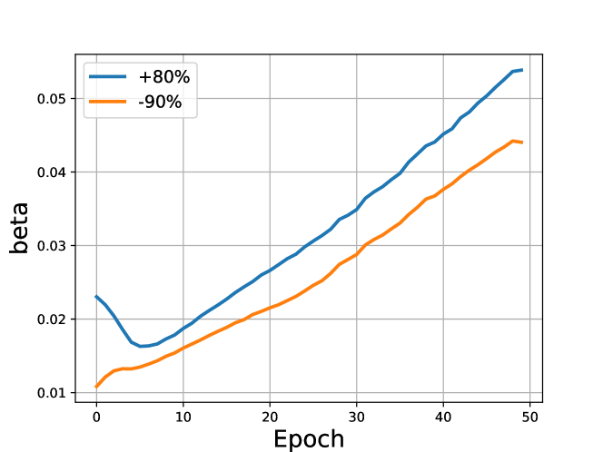
(a) +90%

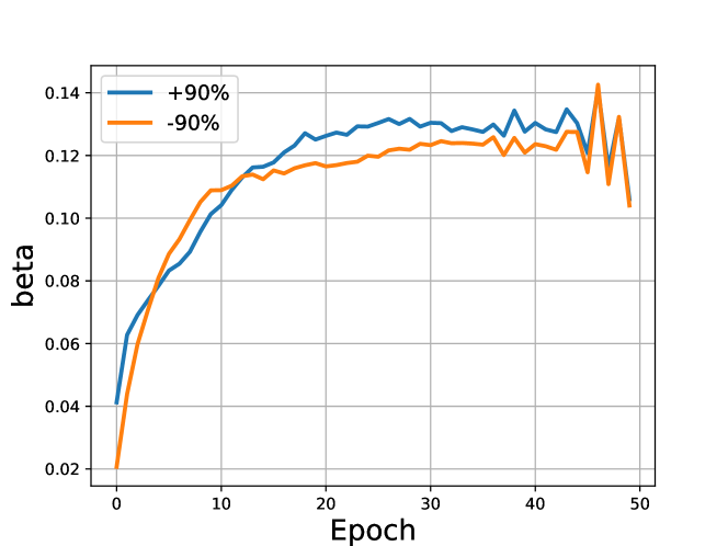
(b) +80%

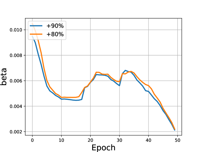
(c) -90%

Figure 5: FedDA_Auto Colored-MNIST

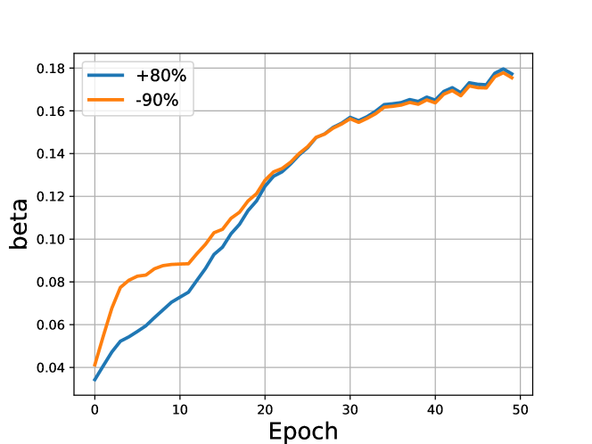
(a) +90%

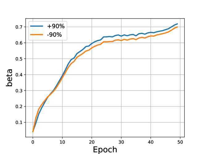
(b) +80%

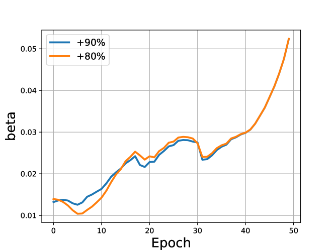
(c) -90%

Figure 6: FedGP_Auto Colored-MNIST

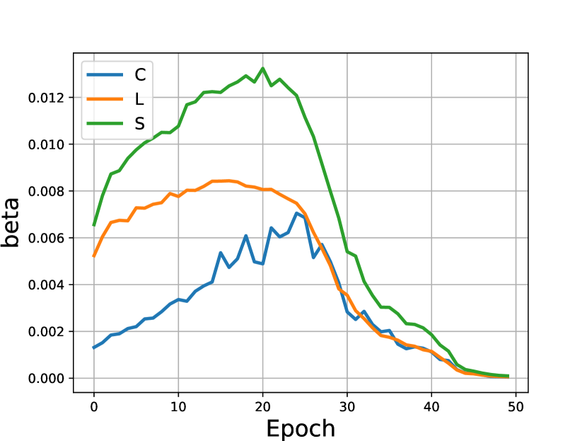
(a) V

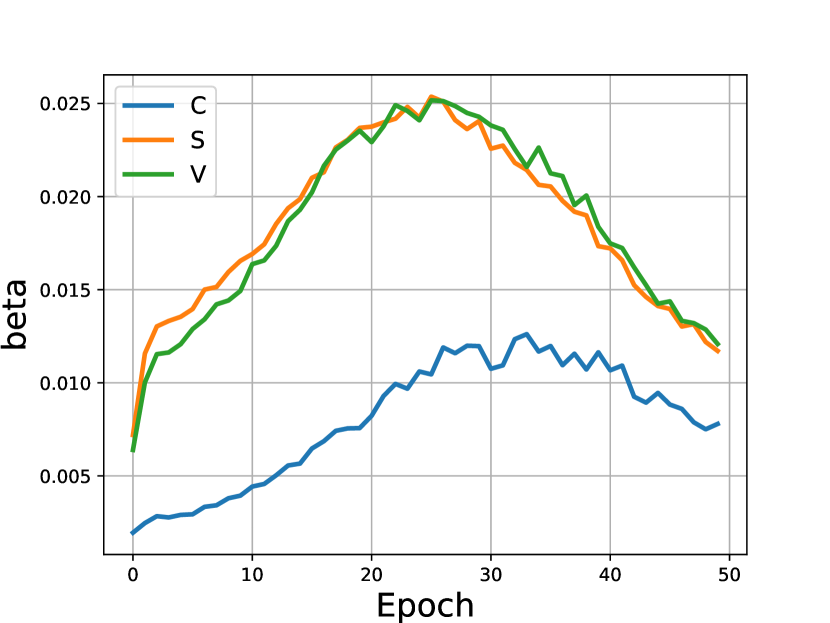
(b) L

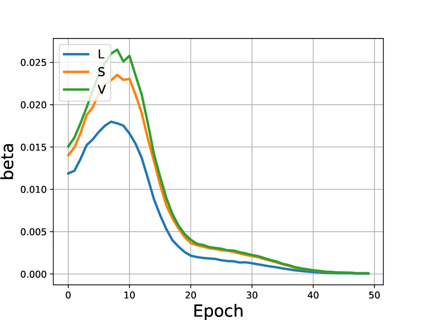
(c) C

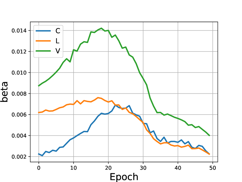
(d) S

Figure 7: FedDA_Auto VLCS

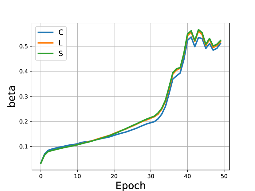
(a) V

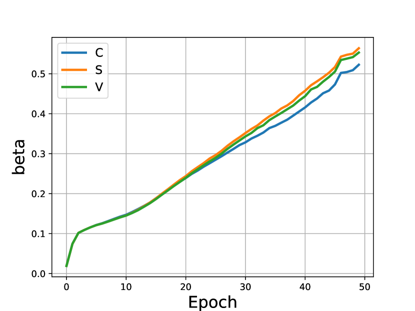
(b) L

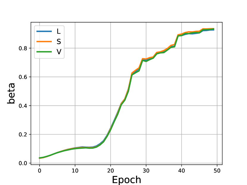
(c) C

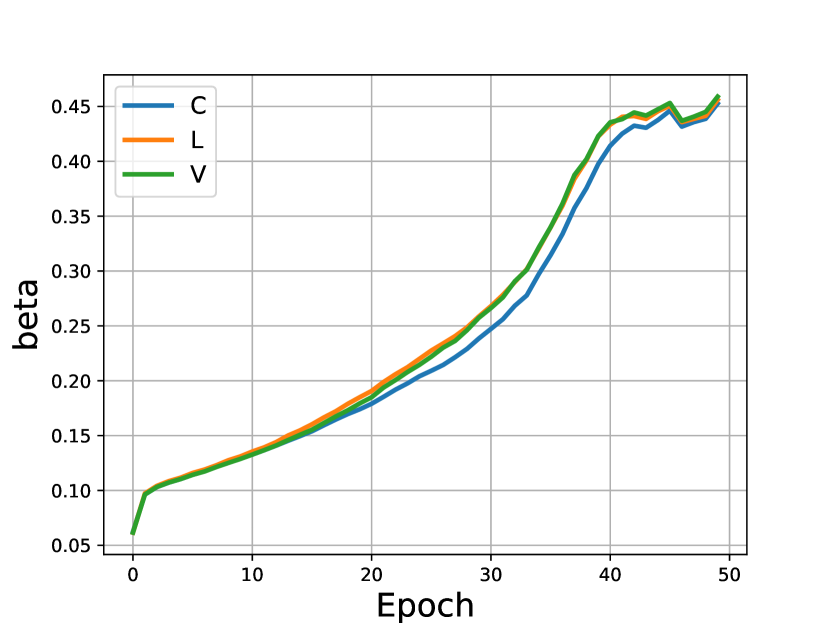
(d) S

Figure 8: FedGP_Auto VLCS

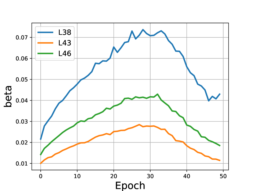
(a) L100

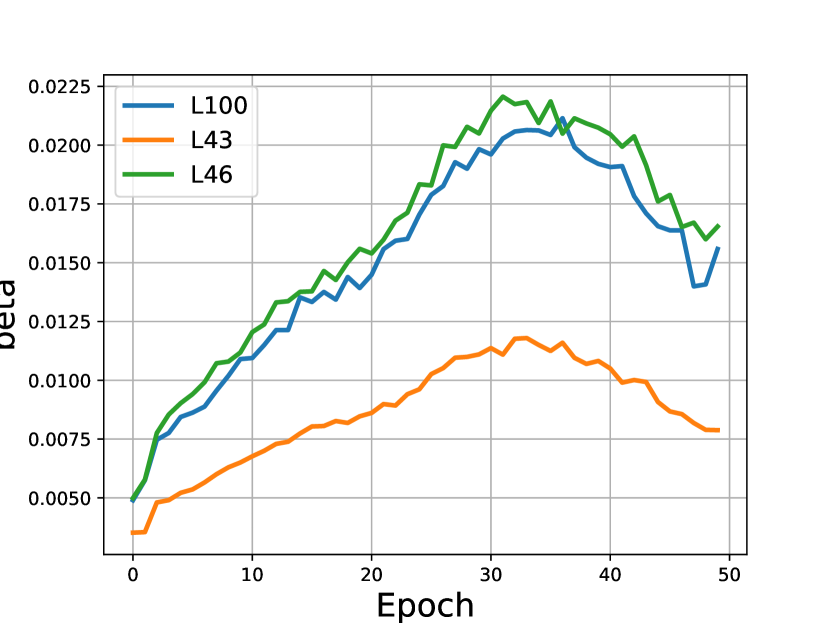
(b) L38

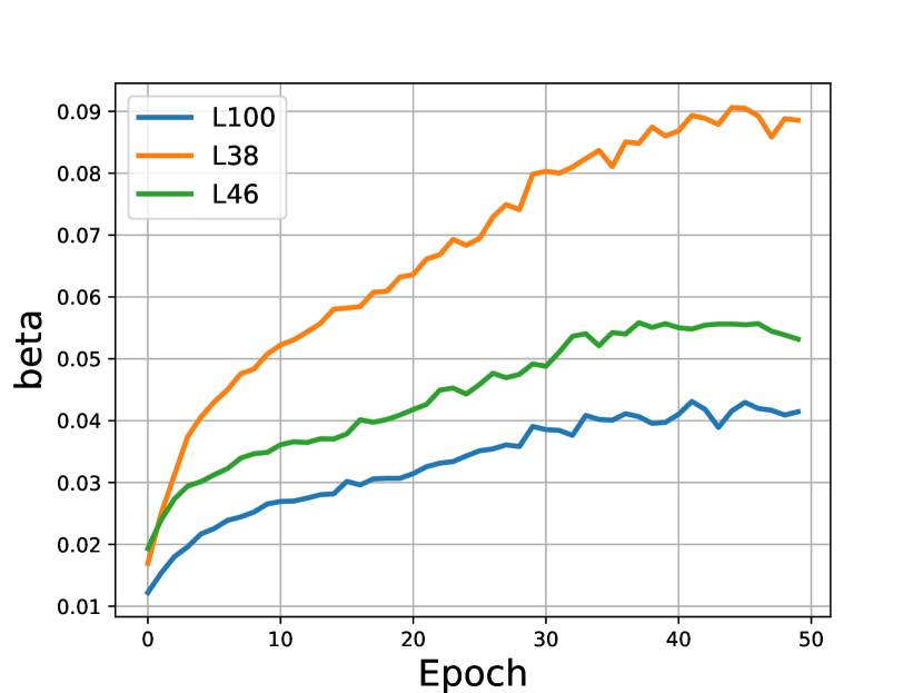
(c) L43

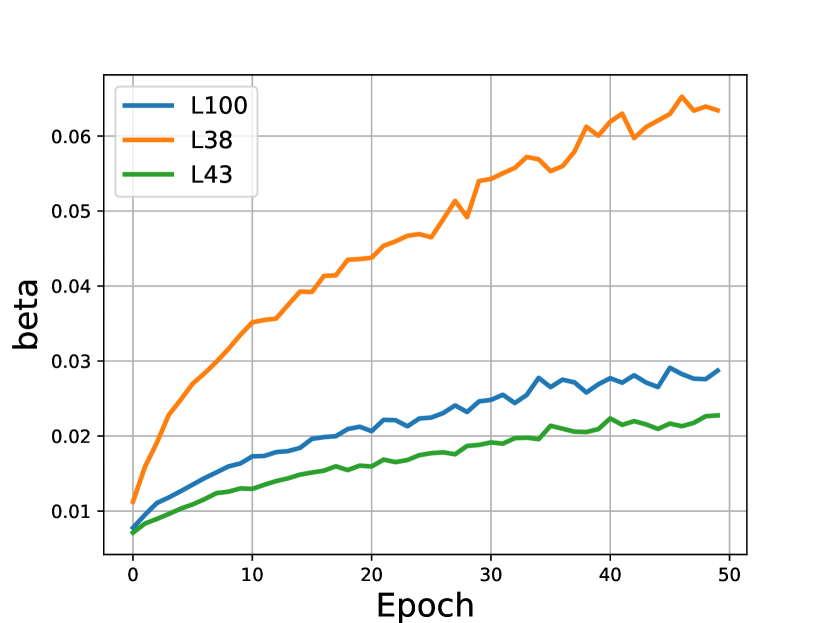
(d) L46

Figure 9: FedDA_Auto TerraIncognita

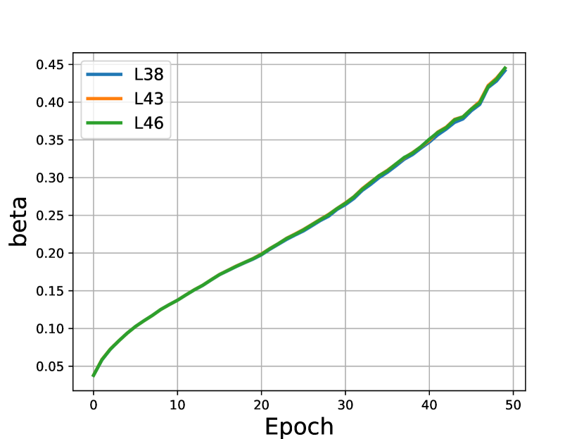
(a) L100

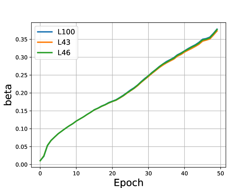
(b) L38

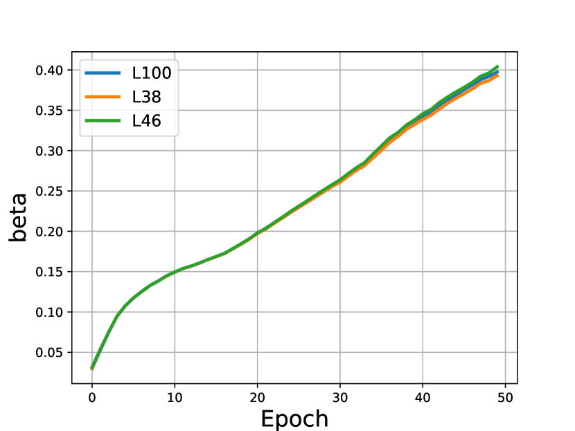
(c) L43

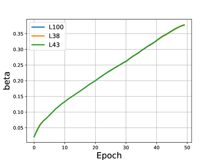
(d) L46

Figure 10: FedGP_Auto TerraIncognita

C.5 Additional Experiment Results on Varying Static Weights ($\beta$)

From the Table 6,  7,  8, and  9, we see FedGP is less sensitive to the choice of the weight parameter $\beta$, enjoying a wider choice range of values, compared with FedDA. Additionally, under fixed weight conditions, FedGP generally outperforms FedDA in most cases.

	0	0.2	0.4	0.6	0.8	1.0
FedDA	61.21	61.10	59.15	49.90	29.80	17.65
FedGP	61.21	63.82	64.30	65.31	64.80	38.48

Table 6: The effect of $\beta$ on FedDA and FedGP on CIFAR-10 dataset with $0.4$ noise level.

-90%	0	0.2	0.4	0.6	0.8	1.0
FedDA	84.41	73.55	54.19	35.16	31.16	27.59
FedGP	84.41	88.96	89.50	89.95	90.03	9.85

Table 7: The effect of $\beta$ on FedDA and FedGP on Colored-MNIST -90% domain.

+90%	0	0.2	0.4	0.6	0.8	1.0
FedDA	88.96	82.37	71.32	62.03	58.77	55.23
FedGP	88.96	89.98	89.76	89.84	90.18	69.47

Table 8: The effect of $\beta$ on FedDA and FedGP on Colored-MNIST +90% domain.

+80%	0	0.2	0.4	0.6	0.8	1.0
FedDA	73.66	75.12	70.21	65.14	61.84	61.32
FedGP	73.66	73.61	74.39	79.32	80.11	76.67

Table 9: The effect of $\beta$ on FedDA and FedGP on Colored-MNIST +80% domain.

C.6 Semi-Synthetic Experiment Settings, Implementation, and Results

In this sub-section, we empirically explore the impact of different extents of domain shifts on FedDA, FedGP, and their auto-weighted version. To achieve this, we conduct a semi-synthetic experiment, where we manipulate the extent of domain shifts by adding different levels of Gaussian noise (noisy features) and degrees of class imbalance (label shifts). We show that the main impact comes from the shifts between target and source domainss instead of the shifts between source domains themselves.

Datasets and models

We create the semi-synthetic distribution shifts by adding different levels of feature noise and label shifts to Fashion-MNIST [29] and CIFAR-10 [16] datasets, adapting from the Non-IID benchmark [17]. For the model, we use a CNN model architecture consisting of two convolutional layers and three fully-connected layers. We set the communication round $R=50$ and the local update epoch to $1$, with $10$ clients (1 target, 9 source clients) in the system.

Baselines

We compare the following methods: Source Only: we only use the source gradients by averaging. Finetune_Offline: we perform the same number of 50 epochs of fine-tuning after FedAvg. FedDA ($\beta=0.5$): a convex combination with a middle trade-off point of source and target gradients. FedGP ($\beta=0.5$): a middle trade-off point between source and target gradients with gradient projection. Target Only: we only use the target gradient ($\beta=0$). Oracle: a fully-supervised training on the labeled target domain serving as the upper bound.

Implementation

For the experiments on the Fashion-MNIST dataset, we set the source learning rate to be $0.01$ and the target learning rate to $0.05$. For CIFAR-10, we use a $0.005$ source learning rate and a $0.0025$ learning rate. The source batch size is set to $64$ and the target batch size is $16$. We partition the data to clients using the same procedure described in the benchmark [17]. We use the cross-entropy loss as the criterion and apply the Adam [15] optimizer.

Setting 1: Noisy features

We add different levels of Gaussian noise to the target domain to control the source-target domain differences. For the Fashion-MNIST dataset, we add Gaussian noise levels of $std=(0.2,0.4,0.6,0.8)$ to input images of the target client, in order to create various degrees of shifts between source and target domains. The task is to predict 10 classes on both source and target clients. For the CIFAR-10 dataset, we use the same noise levels, and the task is to predict 4 classes on both source and target clients. We use 100 labeled target samples for Fashion-MNIST and 10% of the labeled target data for the CIFAR-10 dataset.

Setting 2: Label shifts

We split the Fashion-MNIST into two sets with 3 and 7 classes, respectively, denoted as $D_{1}$ and $D_{2}$. A variable $\eta\in[0,0.5]$ is used to control the difference between source and target clients by defining $D_{S}$ = $\eta$ portion from $D_{1}$ and $(1-\eta)$ portion from $D_{2}$, $D_{T}$ = $(1-\eta)$ portion from $D_{1}$ and $\eta$ portion from $D_{2}$. When $\eta=0.5$, there is no distribution shift, and when $\eta\rightarrow 0$, the shifts caused by label shifts become more severe. We use 15% labeled target samples for the target client. We test on cases with $\eta=[0.45,0.30,0.15,0.10,0.05,0.00]$.

Auto-weighted methods and FedGP maintain a better trade-off between bias and variance

Table 10 and Table 11 display the performance trends of compared methods versus the change of source-target domain shifts. In general, when the source-target domain difference grows bigger, FedDA, Finetune_Offline, and FedAvg degrade more severely compared with auto-weighted methods, FedGP and Target Only. We find that auto-weighted methods and FedGP outperform other baselines in most cases, showing a good ability to balance bias and variances under various conditions and being less sensitive to changing shifts. For the label shift cases, the target variance decreases as the domain shift grows bigger (easier to predict with fewer classes). Therefore, auto-weighted methods, FedGP as well as Target Only surprisingly achieve higher performance with significant shift cases. In addition, auto-weighted FedDA manages to achieve a significant improvement compared with the fixed weight FedDA, with a competitive performance compared with FedGP_Auto, while FedGP_Auto generally has the best accuracy compared with other methods, which coincides with the synthetic experiment results.

Connection with our theoretical insights

Interestingly, we see that when the shift is relatively small ($\eta=0.45$ and 0 noise level for Fashion-MNIST), FedAvg and FedDA both outperform FedGP. Compared with what we have observed from our theory (Figure 2), adding increasing levels of noise can be regarded as going from left to right on the x-axis and when the shifts are small, we probably will get into an area where FedDA is better. When increasing the label shifts, we are increasing the shifts and decreasing the variances simultaneously, we go diagonally from the top-left to the lower-right in Figure 2, where we expect FedAvg is the best when we start from a small domain difference.

Tables of noisy features and label shifts experiments

Table 10 and Table 11 contain the full results. We see that FedGP, FedDA_Auto and FedGP_Auto methods obtain the best accuracy under various conditions; FedGP_Auto outperforms the other two in most cases, which confirms the effectiveness of our weight selection methods suggested by the theory.

	Fashion-MNIST				CIFAR-10
Target noise	0	0.2	0.4	0.6	0.8	0.2	0.4	0.6	0.8
Source Only	83.94	25.49	18.55	16.71	14.99	20.48	17.61	16.44	16.27
Finetune_Offline	81.39	48.26	40.15	36.64	33.71	66.31	56.80	52.10	49.37
FedDA_0.5	86.41	69.73	58.6	50.13	45.51	62.25	54.67	49.77	47.08
FedGP_0.5	76.33	75.09	71.09	68.01	62.22	66.40	65.28	63.29	61.59
FedGP_1	79.40	77.03	71.67	63.71	54.18	21.46	20.75	19.31	18.26
FedDA_Auto	78.37	77.10	72.58	67.78	62.81	65.72	64.43	62.25	60.25
FedGP_Auto	76.22	75.16	71.53	67.53	62.98	67.41	65.17	62.94	61.34
Target Only	74.00	70.59	66.03	61.26	57.82	60.69	60.25	59.38	59.03
Oracle	82.00	82.53	81.20	75.60	72.60	73.61	70.12	69.22	68.50

Table 10: Target domain test accuracy (%) by adding feature noise to Fashion-MNIST and CIFAR-10 datasets using different aggregation rules.

$\eta$	0.45	0.3	0.15	0.1	0.05	0
Source Only	83.97	79.71	69.15	59.90	52.51	0.00
Finetune_Offline	79.84	80.21	83.13	85.43	89.63	33.25
FedDA_0.5	82.44	80.85	77.50	76.51	68.26	59.56
FedGP_0.5	82.97	83.24	85.97	88.72	91.89	98.71
FedGP_1	77.41	73.12	62.54	53.56	27.62	0.00
FedDA_Auto	84.12	84.07	86.42	89.25	92.06	98.44
FedGP_Auto	84.57	84.31	86.67	89.43	92.18	98.45
Target only	81.05	82.44	84.00	88.02	89.80	98.32
Oracle	87.68	88.06	90.56	91.9	93.46	98.73

Table 11: Target domain test accuracy (%) by adding feature noise to the Fashion-MNIST dataset using different aggregation rules.

Impact of extent of shifts between source clients

In addition to the source-target domain differences, we also experiment with different degrees of shifts within source clients. To control the extent of shifts between source clients, we use a target noise $=0.4$ with $[3,5,7,9]$ labels available. From the results, we discover the shifts between source clients themselves have less impact on the target domain performance. For example, the 3-label case (a bigger shift) generally outperforms the 5-label one with a smaller shift. Therefore, we argue that the source-target shift serves as the main influencing factor for the FDA problem.

Number of labels	9	7	3	5
Source Only	11.27	18.81	25.54	34.11
Finetune_Offline	37.79	64.75	68.69	65.41
FedDA_0.5	55.01	57.9	54.16	61.62
FedGP_0.5	68.50	68.64	64.43	66.59
FedGP_1	65.27	59.07	26.37	39.86
Target_Only	63.06	65.76	61.8	63.65
Oracle	81.2	81.2	81.2	81.2

Table 12: Target domain test accuracy (%) on label shifts with [3,5,7,9] labels available on Fashion-MNIST dataset with target noise = 0.4 and 100 target labeled samples.

C.7 Additional Ablation Study Results

The effect of target gradient variances

We conduct experiments with increasing numbers of target samples (decreased target variances) with varying noise levels $[0.2,0.4,0.6]$ on Fashion-MNIST and CIFAR-10 datasets with 10 clients in the system. We compare two aggregation rules FedGP and FedDA, as well as their auto-weighted versions. The results are shown in Table 13 (fixed FedDA and FedGP) and Table 14 (auto-weighted FedDA and FedGP). When the number of available target samples increases, the target performance also improves. For the static weights, we discover that FedGP can predict quite well even with a small number of target samples, especially when the target variance is comparatively small. For auto-weighted FedDA and FedGP, we find they usually have higher accuracy compared with FedGP, which further confirms our auto-weighted scheme is effective in practice. Also, we observe that sometimes FedDA_Auto performs better than FedGP_Auto (e.g. on the Fashion-MNIST dataset) and sometimes vice versa (e.g. on the CIFAR-10 dataset). We hypothesize that since the estimation of variances for FedGP is an approximation instead of the equal sign, it is possible that FedDA_Auto can outperform FedGP_Auto in some cases because of more accurate estimations of the auto weights $\beta$. Also, we notice auto-weighted scheme seems to improve the performance more when the target variance is smaller with more available samples and the source-target shifts are relatively small.

Noise level		0.2		0.4		0.6
		FedDA	FedGP	FedDA	FedGP	FedDA	FedGP
Fashion-MNIST	100	69.73	75.09	58.6	71.09	50.13	68.01
	200	72.07	74.21	58.59	70.93	52.67	70.31
	500	76.59	78.41	65.34	74.07	54.97	70.52
	1000	77.92	78.68	68.26	75.17	59.16	71.63
CIFAR-10	5%	62.24	64.21	46.89	63.57	47.56	61.39
	10%	62.25	65.92	54.67	65.39	49.77	63.67
	15%	59.16	65.97	56.93	65.11	51.83	63.73

Table 13: Target domain test accuracy (%) by adding feature noise=0.2, 0.4, 0.6 on the Fashion-MNIST and CIFAR-10 datasets with different numbers of available target samples using fixed weights.

Noise level		0.2		0.4		0.6
		FedDA_Auto	FedGP_Auto	FedDA_Auto	FedGP_Auto	FedDA_Auto	FedGP_Auto
Fashion-MNIST	100	79.04	75.45	72.21	71.93	66.16	67.47
	200	79.74	76.74	74.30	72.96	69.27	69.04
	500	79.48	78.65	75.21	74.55	71.40	70.72
	1000	80.23	79.91	76.75	76.35	73.16	73.16
CIFAR-10	5%	63.04	65.62	60.79	62.84	60.02	60.47
	10%	65.72	67.41	64.43	65.17	62.25	62.94
	15%	66.57	67.56	65.4	65.92	63.36	63.14

Table 14: Target domain test accuracy (%) by adding feature noise=0.2, 0.4, 0.6 on the Fashion-MNIST and CIFAR-10 datasets with different numbers of available target samples using auto weights.

C.8 Implementation Details of FedGP

To implement fine-grained projection for the real model architecture, we compute the cosine similarity between one source client gradient $g_{i}$ and the target gradient $g_{T}$ for each layer of the model with a threshold of 0. In addition, we align the magnitude of the gradients according to the number of target/source samples, batch sizes, local updates, and learning rates. In this way, we implement FedGP by projecting the target gradient towards source directions. We show the details of implementing static and auto-weighted versions of FedGP in the following two paragraphs.

Static-weighted FedGP implementation

Specifically, we compute the model updates from source and target clients as $G_{S_{i}}^{(r)}\simeq h_{S_{i}}^{(r)}-h_{global}^{(r-1)}$ and $G_{T}^{(r)}\simeq h_{T}^{(r)}-h_{T}^{(r-1)}$, respectively. In our real training process, because we use different learning rates, and training samples for source and target clients, we need to align the magnitude of model updates. We first align the model updates from source clients to the target client and combine the projection results with the target updates. We use $lr_{T}$ and $lr_{S}$ to denote the target and source learning rates; $batchsize_{T}$ and $batchsize_{S}$ are the batch sizes for target and source domains, respectively; $n_{l}$ is the labeled sample size on target client and $n_{i}$ is the sample size for source client $\mathcal{C}_{S_{i}}$; $r_{S}$ is the rounds of local updates on source clients. The total gradient projection $P_{GP}$ from all source clients $\{G_{S_{i}}^{(r)}\}_{i=1}^{N}$ projected on the target direction $G_{T}$ could be computed as follows. We use $\mathcal{L}$ to denote all layers of current model updates. $n_{i}$ denotes the number of samples trained on source client $\mathcal{C}_{S_{i}}$, which is adapted from FedAvg [22] to redeem data imbalance issue. Hence, we normalize the gradient projections according to the number of samples. Also, $\bigcup^{\mathcal{L}}_{l\in\mathcal{L}}$ concatenates the projected gradients of all layers.

$$P_{GP}=\bigcup_{l\in\mathcal{L}}\sum_{i=1}^{N}\left(\mathbf{GP}\left(\left(h_{S_{i}}^{(r)}-h_{global}^{(r-1)}\right)^{l},\left(h_{T}^{(r)}-h_{T}^{(r-1)}\right)^{l}\right)\cdot\frac{n_{i}}{\sum^{N}_{i}n_{i}}\cdot\frac{\frac{n_{l}}{batchsize_{T}}}{\frac{n_{i}}{batchsize_{S}}}\cdot\frac{lr_{T}}{lr_{S}}\cdot\frac{1}{r_{S}}\cdot\left(h_{S_{i}}^{(r)}-h_{global}^{(r-1)}\right)\right)$$ (108)

Lastly, a hyper-parameter $\beta$ is used to incorporate target update $G_{T}$ into $P_{GP}$ to have a more stable performance. The final target model weight $h_{T}^{(r)}$ at round $r$ is thus expressed as:

$$h_{T}^{(r)}=h_{T}^{(r-1)}+(1-\beta)\cdot P_{GP}+\beta\cdot G_{T}$$ (109)

Auto-weighted FedGP Implementation

For auto-weighted scheme for FedGP, we compute a dynamic weight $\beta_{i}$ for each source domain $\mathcal{D}_{S_{i}}$ per communication round. With a set of pre-computed $\{\beta_{i}\}^{N}_{i=1}$ weight values, the weighted projected gradients for a certain epoch can be expressed as follows:

$$P_{GP}=\bigcup_{l\in\mathcal{L}}\sum_{i=1}^{N}\left(\mathbf{GP}\left(\left(h_{S_{i}}^{(r)}-h_{global}^{(r-1)}\right)^{l},\left(h_{T}^{(r)}-h_{T}^{(r-1)}\right)^{l}\right)\cdot\frac{n_{i}\cdot\beta_{i}}{\sum^{N}_{i}n_{i}}\cdot\frac{\frac{n_{l}}{batchsize_{T}}}{\frac{n_{i}\cdot\beta_{i}}{batchsize_{S}}}\cdot\frac{lr_{T}}{lr_{S}}\cdot\frac{1}{r_{S}}\cdot\left(h_{S_{i}}^{(r)}-h_{global}^{(r-1)}\right)\right)$$ (110)

Similarly, we need to incorporate target update $G_{T}$ into $P_{GP}$. The final target model weight $h_{T}^{(r)}$ at round $r$ is thus expressed as:

$$h_{T}^{(r)}=h_{T}^{(r-1)}+P_{GP}+\frac{n_{i}\cdot\beta_{i}}{\sum^{N}_{i}n_{i}}\cdot G_{T}$$ (111)

C.9 Gradient Projection Method’s Time and Space Complexity

Time complexity: Assume the total parameter is $m$ and we have $l$ layers. To make it simpler, assume each layer has an average of $\frac{m}{l}$ parameters. Computing cosine similarity for all layers of one source client is $O((\frac{m}{l})^{2}\cdot l)=O(m^{2}/l)$. We have $N$ source clients so the total time cost for GP is $O(N\cdot m^{2}/l)$.

Space complexity: The extra memory cost for GP (computing cosine similarity) is $O(1)$ per client for storing the current cosine similarity value. In a real implementation, the whole process of projection is fast, with around $~{}0.023$ seconds per call needed for $N=10$ clients of Fashion-MNIST experiments on the NVIDIA TITAN Xp hardware with GPU available.

C.10 Comparison with the Unsupervised FDA Method

In this sub-section, we show the performances of our methods compared with the SOTA unsupervised FDA method KD3A [8]. However, we note that our setting with limited target data is different from the unsupervised FDA setting which assumes there exists abundant unlabeled data on the target domain. As shown in Table 15, though sometimes KD3A [8] outperforms our methods and is fairly close to Oracle performances with comparatively small shift cases (VLCS dataset), in other cases, training on all unlabeled data seems to fail especially for the large shift cases (TerraIncognita dataset). Also, auto-weighted FedDA and FedGP generally outperform KD3A in most cases and on average.

	VLCS					TerraIncognita
	C	L	V	S	Avg	L100	L38	L43	L46	Avg
KD3A [8]	99.64	63.28	78.07	80.49	79.01	62.24	37.19	28.09	28.40	38.98
FedGP	99.43	71.09	73.65	78.70	80.72	81.46	77.75	64.18	61.56	71.24
FedDA_Auto	99.41	70.99	75.38	80.08	81.46	79.06	78.59	66.02	63.37	71.76
FedGP_Auto	99.48	70.71	75.24	79.99	81.36	78.70	78.28	65.55	63.78	71.58
Oracle	100.00	72.72	78.65	82.71	83.52	96.41	95.01	91.98	89.04	93.11

Table 15: Performance comparison with the unsupervised SOTA method.

C.11 Comparison with the Semi-Supervised Domain Adaptation (SSDA) Method

In this sub-section, we show the performances of our methods compared with SSDA methods. However, we note that the suggested SSDA methods cannot be directly adapted to the federated setting without major modification.  Kim and Kim, [14] uses feature alignments and requires access to the source and target data at the same time, which is usually difficult to achieve in federated learning. As for  Saito et al., [25], the overall adversarial learning objective functions consist of a loss objective on both source and target labeled data and the entropy coming from the unlabeled target data, which also cannot be directly adapted to federated learning. On the contrary, auto-weighted methods and FedGP have the flexibility to do the single source-target domain adaptation, which can be compared with the SSDA method, though we notice that our setting is different from SSDA since we do not have unlabeled data on the target domain and do not leverage the information coming from this set of data. Here, we perform experiments on real-world datasets: our results suggest that auto-weighted methods and FedGP outperform MME [25] when the shifts are large even without using unlabeled data (overall our proposed methods have a comparable performance with MME). Also, we observe in a single source-target domain adaptation setting, auto-weighted FedGP usually has a better performance than auto-weighted FedDA and FedGP.

	0 ->1 / 1 ->0	0 ->2 / 2 ->0	1 ->2 / 2 ->1
MME [25]	79.55 / 89.28	25.98 / 12.99	14.66 / 24.43
FedGP	79.34 / 88.34	90.23 / 64.47	90.23 / 78.70
FedDA_Auto	79.31 / 88.38	87.00 / 56.07	89.13 / 66.59
FedGP_Auto	79.34 / 71.59	90.23 / 80.95	90.23 / 79.34

Table 16: Colored-MNIST (0: +90%, 1: +80%, 2: -90%)

	0->1	1->2	2->3
MME [25]	68.68	72.86	81.90
FedGP	67.92	75.30	77.45
FedDA_Auto	67.92	75.73	76.97
FedGP_Auto	68.45	74.21	77.69

Table 17: VLCS (0: C, 1: L, 2: V, 3: S)

	0->1	1->2	2->3
MME [25]	74.51	54.91	58.50
FedGP	72.35	58.19	60.03
FedDA_Auto	72.31	54.26	61.33
FedGP_Auto	72.42	56.27	61.90

Table 18: TerraIncognita (0: L100, 1: L38, 2: L43, 3: L46)

References

- Arjovsky et al., [2019] Arjovsky, M., Bottou, L., Gulrajani, I., and Lopez-Paz, D. (2019). Invariant risk minimization. arXiv preprint arXiv:1907.02893.
- Beery et al., [2018] Beery, S., Van Horn, G., and Perona, P. (2018). Recognition in terra incognita. In Proceedings of the European conference on computer vision (ECCV), pages 456–473.
- Cao et al., [2021] Cao, X., Fang, M., Liu, J., and Gong, N. (2021). Fltrust: Byzantine-robust federated learning via trust bootstrapping. In Proceedings of NDSS.
- Collins et al., [2021] Collins, L., Hassani, H., Mokhtari, A., and Shakkottai, S. (2021). Exploiting shared representations for personalized federated learning. In International Conference on Machine Learning, pages 2089–2099. PMLR.
- Deng, [2012] Deng, L. (2012). The mnist database of handwritten digit images for machine learning research. IEEE Signal Processing Magazine, 29(6):141–142.
- Deng et al., [2020] Deng, Y., Kamani, M. M., and Mahdavi, M. (2020). Adaptive personalized federated learning. arXiv preprint arXiv:2003.13461.
- Fang et al., [2013] Fang, C., Xu, Y., and Rockmore, D. N. (2013). Unbiased metric learning: On the utilization of multiple datasets and web images for softening bias. In Proceedings of the IEEE International Conference on Computer Vision, pages 1657–1664.
- Feng et al., [2021] Feng, H., You, Z., Chen, M., Zhang, T., Zhu, M., Wu, F., Wu, C., and Chen, W. (2021). Kd3a: Unsupervised multi-source decentralized domain adaptation via knowledge distillation. In Meila, M. and Zhang, T., editors, Proceedings of the 38th International Conference on Machine Learning, volume 139 of Proceedings of Machine Learning Research, pages 3274–3283. PMLR.
- Gulrajani and Lopez-Paz, [2020] Gulrajani, I. and Lopez-Paz, D. (2020). In search of lost domain generalization. In International Conference on Learning Representations.
- He et al., [2021] He, C., Yang, Z., Mushtaq, E., Lee, S., Soltanolkotabi, M., and Avestimehr, S. (2021). Ssfl: Tackling label deficiency in federated learning via personalized self-supervision. arXiv preprint arXiv:2110.02470.
- He et al., [2016] He, K., Zhang, X., Ren, S., and Sun, J. (2016). Deep residual learning for image recognition. In Proceedings of the IEEE conference on computer vision and pattern recognition, pages 770–778.
- Jeong et al., [2020] Jeong, W., Yoon, J., Yang, E., and Hwang, S. J. (2020). Federated semi-supervised learning with inter-client consistency & disjoint learning. In International Conference on Learning Representations.
- Karimireddy et al., [2020] Karimireddy, S. P., Kale, S., Mohri, M., Reddi, S., Stich, S., and Suresh, A. T. (2020). SCAFFOLD: Stochastic controlled averaging for federated learning. In III, H. D. and Singh, A., editors, Proceedings of the 37th International Conference on Machine Learning, volume 119 of Proceedings of Machine Learning Research, pages 5132–5143. PMLR.
- Kim and Kim, [2020] Kim, T. and Kim, C. (2020). Attract, perturb, and explore: Learning a feature alignment network for semi-supervised domain adaptation. In Computer Vision–ECCV 2020: 16th European Conference, Glasgow, UK, August 23–28, 2020, Proceedings, Part XIV 16, pages 591–607. Springer.
- Kingma and Ba, [2014] Kingma, D. P. and Ba, J. (2014). Adam: A method for stochastic optimization. arXiv preprint arXiv:1412.6980.
- Krizhevsky et al., [2009] Krizhevsky, A., Hinton, G., et al. (2009). Learning multiple layers of features from tiny images.
- Li et al., [2022] Li, Q., Diao, Y., Chen, Q., and He, B. (2022). Federated learning on non-iid data silos: An experimental study. In IEEE International Conference on Data Engineering.
- Li et al., [2021] Li, T., Hu, S., Beirami, A., and Smith, V. (2021). Ditto: Fair and robust federated learning through personalization. In International Conference on Machine Learning, pages 6357–6368. PMLR.
- Li et al., [2020] Li, X., Gu, Y., Dvornek, N., Staib, L. H., Ventola, P., and Duncan, J. S. (2020). Multi-site fmri analysis using privacy-preserving federated learning and domain adaptation: Abide results. Medical Image Analysis, 65:101765.
- Liang et al., [2020] Liang, J., Hu, D., and Feng, J. (2020). Do we really need to access the source data? Source hypothesis transfer for unsupervised domain adaptation. In III, H. D. and Singh, A., editors, Proceedings of the 37th International Conference on Machine Learning, volume 119 of Proceedings of Machine Learning Research, pages 6028–6039. PMLR.
- Marfoq et al., [2022] Marfoq, O., Neglia, G., Vidal, R., and Kameni, L. (2022). Personalized federated learning through local memorization. In International Conference on Machine Learning, pages 15070–15092. PMLR.
- McMahan et al., [2017] McMahan, B., Moore, E., Ramage, D., Hampson, S., and Arcas, B. A. y. (2017). Communication-Efficient Learning of Deep Networks from Decentralized Data. In Singh, A. and Zhu, J., editors, Proceedings of the 20th International Conference on Artificial Intelligence and Statistics, volume 54 of Proceedings of Machine Learning Research, pages 1273–1282. PMLR.
- Nguyen et al., [2021] Nguyen, T., Le, T., Zhao, H., Tran, Q. H., Nguyen, T., and Phung, D. (2021). Most: Multi-source domain adaptation via optimal transport for student-teacher learning. In Uncertainty in Artificial Intelligence, pages 225–235. PMLR.
- Peng et al., [2020] Peng, X., Huang, Z., Zhu, Y., and Saenko, K. (2020). Federated adversarial domain adaptation. In International Conference on Learning Representations.
- Saito et al., [2019] Saito, K., Kim, D., Sclaroff, S., Darrell, T., and Saenko, K. (2019). Semi-supervised domain adaptation via minimax entropy. ICCV.
- Saito et al., [2018] Saito, K., Watanabe, K., Ushiku, Y., and Harada, T. (2018). Maximum classifier discrepancy for unsupervised domain adaptation. In Proceedings of the IEEE conference on computer vision and pattern recognition, pages 3723–3732.
- Wang et al., [2019] Wang, H., Yurochkin, M., Sun, Y., Papailiopoulos, D., and Khazaeni, Y. (2019). Federated learning with matched averaging. In International Conference on Learning Representations.
- Wu and Gong, [2021] Wu, G. and Gong, S. (2021). Collaborative optimization and aggregation for decentralized domain generalization and adaptation. In Proceedings of the IEEE/CVF International Conference on Computer Vision (ICCV), pages 6484–6493.
- Xiao et al., [2017] Xiao, H., Rasul, K., and Vollgraf, R. (2017). Fashion-mnist: a novel image dataset for benchmarking machine learning algorithms. arXiv preprint arXiv:1708.07747.
- [30] Xie, C., Koyejo, S., and Gupta, I. (2020a). Zeno++: Robust fully asynchronous SGD. In III, H. D. and Singh, A., editors, Proceedings of the 37th International Conference on Machine Learning, volume 119 of Proceedings of Machine Learning Research, pages 10495–10503. PMLR.
- [31] Xie, M., Long, G., Shen, T., Zhou, T., Wang, X., Jiang, J., and Zhang, C. (2020b). Multi-center federated learning.
- Yang et al., [2021] Yang, D., Xu, Z., Li, W., Myronenko, A., Roth, H. R., Harmon, S., Xu, S., Turkbey, B., Turkbey, E., Wang, X., et al. (2021). Federated semi-supervised learning for covid region segmentation in chest ct using multi-national data from china, italy, japan. Medical image analysis, 70:101992.
- Zhao et al., [2018] Zhao, H., Zhang, S., Wu, G., Moura, J. M., Costeira, J. P., and Gordon, G. J. (2018). Adversarial multiple source domain adaptation. Advances in neural information processing systems, 31.