Exploiting Sparsity in Pruned Neural Networks to Optimize Large Model Training

Abstract

Parallel training of neural networks at scale is challenging due to significant overheads arising from communication. Recently, deep learning researchers have developed a variety of pruning algorithms that are capable of pruning (i.e. setting to zero) 80-90% of the parameters in a neural network to yield sparse subnetworks that equal the accuracy of the unpruned parent network. In this work, we propose a novel approach that exploits these sparse subnetworks to optimize the memory utilization and communication in two popular algorithms for parallel deep learning namely – data and inter-layer parallelism. We integrate our approach into AxoNN, a highly scalable framework for parallel deep learning that relies on data and inter-layer parallelism, and demonstrate the reduction in communication time and memory utilization. On 512 NVIDIA V100 GPUs, our optimizations reduce the memory consumption of a 2.7 billion parameter model by 74%, and the total communication time by 40%, thus providing an overall speedup of 34% over AxoNN, 32% over DeepSpeed-3D and 46% over Sputnik, a sparse matrix computation baseline.

I Introduction

Deep learning researchers have observed that increasing the size of a neural network almost always leads to better generalization i.e., accuracies on test data [1]. This has led to the development of neural architectures with billions of parameters [2], which are naturally trained in parallel on large GPU clusters due to their extreme compute and memory requirements. The progressive increase in neural network sizes has necessitated a corresponding increase in the number of GPUs to train them. However, with increasing GPU counts, communication becomes a significant bottleneck in the training procedure. Thus, designing algorithms that can improve the efficiency of training at scale is extremely critical. This will ensure that we can harness the proven benefits of growing network sizes while being able to train them in a reasonable amount of time.

The number of parameters in contemporary deep learning models is often in the tens to hundreds of billions. In their work on the lottery ticket hypothesis (LTH), Frankle et al. observe empirically that a large fraction of the parameter set (80-90%) can be pruned (set to zero) at initialization without affecting the generalization performance on test data [3]. Subsequently, this phenomenon has witnessed great interest from the deep learning community and several follow up studies have tried to further refine the hypothesis, propose efficient pruning algorithms and/or prove it for a broader class of neural network architectures [4, 5, 6, 7, 8, 9].

Pruning algorithms output extremely sparse subnetworks, which in theory require significantly fewer number of floating point operations as compared to the unpruned networks. Several sparse matrix multiplication kernels for GPUs have been proposed that are specifically optimized for the patterns of sparsities in these subnetworks [10, 11, 12]. However, in spite of the advancements, these approaches are significantly slower than cuBLAS, a popular library for dense matrix multiplications on NVIDIA GPUs (used by deep learning frameworks such as PyTorch and Tensorflow). In Figure 1, we demonstrate that computing a fully connected layer with 90% sparsity using cuBLAS (we fill out zeros explicitly in the dense matrix) is 6–22$\times$ faster than using Sputnik [11], a state-of-the-art sparse matrix multiplication library for deep learning workloads. This suggests that utilizing sparse matrix libraries to improve training performance is currently infeasible.

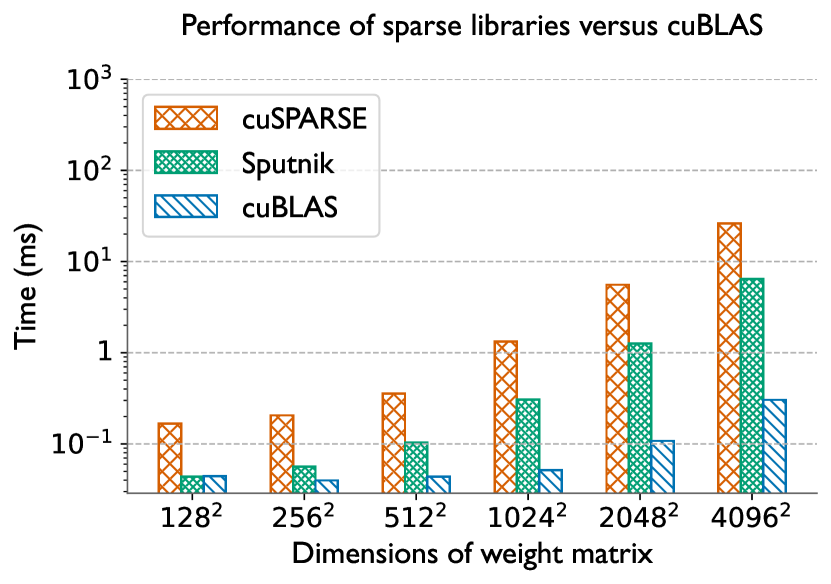
Figure 1: Comparison of the execution times of a fully-connected (FC) layer with a randomly generated, 90% sparse, square weight matrix in mixed precision. FC layers compute a linear transform of their input and are a vital component of various neural network architectures such as transformers[2]. For dense GPU kernels, we use NVIDIA’s cuBLAS, whereas for sparse GPU kernels, we use NVIDIA’s cuSPARSE and Sputnik [11]. We fix the input batch size to 576 and vary the size of the weight matrix from $128^{2}$ to $4096^{2}$.

Instead of trying to optimize computation times, in this work, we focus on exploiting sparsity to optimize memory utilization, and then exploit the saved memory to optimize communication. We demonstrate how our optimizations can greatly reduce the communication times of two widely used parallel algorithms for deep learning – namely inter-layer parallelism (point-to-point communication) and data parallelism (collective communication). First, we propose a novel approach, which we call Sparsity-aware Memory Optimization (SAMO), that provides memory savings of around 66-78%, while still being compute efficient. Through analytical communication models as well as experiments, we demonstrate that these memory savings can be utilized to reduce both the message transmission time as well as the pipeline latency (often called “bubble” time) of inter-layer parallelism. Finally, for data parallelism we only communicate the gradients corresponding to the non-zero (or unpruned) parameters, decreasing the message sizes, and thus alleviating the bottleneck of expensive all-reduce communication.

To demonstrate the efficacy of our optimizations, we integrate our method in AxoNN [13], a highly scalable framework for parallel deep learning that implements an efficient hybrid of data and inter-layer parallelism. On GPT-3 2.7B [2], a 2.7 billion parameter model, we demonstrate that SAMO reduces the memory consumption by 74% (from 80.16 GB to 20.28 GB)! Then, for a strong scaling run of the same model on 128-512 V100 GPUs of Summit, we successfully exploit the freed up memory to reduce the portion of batch spent in communication. We show that the absolute reduction in the communication time accounts for 40% of AxoNN’s batch time on 512 GPUs. This makes our method a significant 34% faster than AxoNN, 32% faster than DeepSpeed-3D [14], and 46% faster that Sputnik [11]. Since Sputnik is designed for single GPU executions, we integrate it in AxoNN to run it in parallel.

We summarize the important contributions of this work below:

• We present Sparsity-aware Memory Optimization (SAMO), a novel method that exploits recently proposed accuracy-preserving parameter pruning algorithms in deep learning, to significantly reduce the memory consumption of neural network training while not sacrificing performance.

• Through analytical communication models and experiments, we demonstrate how these memory savings can be utilized to significantly improve the communication performance of two popular algorithms for parallel deep learning, data and inter-layer parallelism.

• We conduct strong scaling experiments using popular convolution neural network architectures and transformer-based language models with 1.3 to 13 billion parameters on 16 to 2048 GPUs, and demonstrate significant improvements in communication times when compared with two highly scalable parallel deep learning frameworks AxoNN and DeepSpeed-3D.

II Background and Related Work

Below, we provide background on neural network pruning, sparse matrix multiplications, and parallel deep learning.

II-A Over-parameterization in neural networks

We call a neural network over-parameterized, when its size is extremely large as compared to the training dataset. It has been empirically observed that the more over-parameterized a neural network gets, the better it seems to generalize on a held out test dataset [1]. Indeed, the largest neural networks in deep learning (like the GPT-3 [2]) are massively over-parameterized. This perplexing phenomenon, that cannot be explained by classical machine learning, has been an active area of research in deep learning  [15, 16, 17, 1, 18, 19].

II-B Lottery ticket hypothesis

Proposed by Frankle et al. [3]., the lottery ticket hypothesis (LTH) asserts that in a randomly-initialized, over-parameterized neural network, there exists a subnetwork with one- to two-tenths of the parameters, which when trained in isolation can match and even improve the test-set performance of the original neural network. They theorize that in an over-parameterized network, it is this subnetwork that effectively ends up being trained, thus preventing over-fitting. They also present a simple algorithm to identify this subnetwork. Several follow up studies have tried to further refine the hypothesis, propose efficient pruning algorithms and/or prove it for a broader class of neural network architectures [4, 5, 6, 7, 8, 9]. In this work, we use You et al.’s algorithm for pruning [4].

II-C Accelerated sparse kernels

NVIDIA’s cuSPARSE is designed for sparse matrices seen in scientific applications which have extremely high sparsities ($>$99%). Therefore, it is not a suitable candidate for the kinds of sparsities observed in neural network pruning ($<$90%). A number of approaches have been proposed that can operate in these levels of sparsities. Yang et al. augment merge-based algorithms with a novel row-based splitting technique to hide memory access latency [12]. Hong et al. design spMM and sDDMM (used for backward pass of a fully connected layer) that exploit an adaptive tiling strategy to reduce global memory access [10]. Gale et al. conduct an extensive survey of the sparsity patterns found in matrices across a variety of deep learning workloads [20]. Using the insights drawn from this study, they design state-of-the-art sparse kernels for spMM and sDDMM for deep learning workloads [11]. A number of approaches have been proposed that enforce a certain sparsity structure. Gray et al. design GPU kernels for block sparse matrices [21]. Chen et al. propose a novel column-vector-sparse-encoding for block sparse matrices that provides speedup over cuBLAS at sparsities as low as 70% at mixed precision [22]. Dao et al. propose a technique to reduce linear maps to a product of diagonal block sparse matrices and design kernels for computing their products efficiently [23, 24].

II-D Types of parallelism in deep learning

Three kinds of parallelism, namely intra-layer, inter-layer and data parallelism have been proposed in parallel deep learning. Intra-layer parallelism divides the execution of each layer across GPUs [25]. Inter-layer parallelism assigns a contiguous subset of neural network layers to each GPU [26, 27, 28]. Data parallelism creates a replica of the entire network on each GPU [29, 30]. Usually, frameworks for parallel deep learning implement a hybrid of data parallelism with one or both of intra- and inter-layer parallelism [29, 14, 28]. For more details, we refer the reader to Ben-Nun et al. [31].

II-E The AxoNN deep learning framework

In this paper, we implement our ideas in a state-of-the-art framework, AxoNN, for parallel deep learning [13]. AxoNN implements a hybrid of inter-layer and data parallelism. It divides the set of GPUs into $G_{\mathit{data}}$ groups. Each of these groups operates on an equal sized shard of the input batch, thus implementing data parallelism. Within each group, there are $G_{\mathit{inter}}$ GPUs implementing inter-layer parallelism. To achieve concurrency within this inter-layer parallel groups, AxoNN breaks up the input batch shard into several “microbatches” and processes them in a pipelined fashion. Activations and gradients for a microbatch are exchanged among neighboring GPUs using point-to-point communication. As compared to other frameworks, AxoNN optimizes this communication by employing i. asynchronous messaging ii. message driven scheduling of microbatch operations. The former allows it to overlap communication with computation, whereas the latter allows it to reduce pipeline stalls. AxoNN supports mixed precision training [32] and activation checkpointing [33].

III Sparsity-aware Memory Optimization

In this section, we discuss our approach to exploit sparse networks generated by pruning methods to significantly reduce the memory consumption of large model training. We refer to our approach as Sparsity-aware Memory Optimization (SAMO). We discuss SAMO in the context of mixed-precision training[32], which is the predominant mode used for the training of large multi billion-parameter models [29, 34, 35]. However, the optimizations discussed below are general and can also be applied to single-precision training.

Mixed-precision training involves storing the model parameters and gradients in both 16-bit (half-precision) and 32-bit (single-precision), and the optimizer states in 32-bit. The expensive forward and the backward pass are computed in 16-bit for efficiency, whereas the relatively cheaper optimizer step is done in 32-bit for accuracy. For more details, we refer the reader to Micikevicius et al. [32].

Model parameters, gradients and optimizer states are collectively referred to as the model state [29]. While mixed-precision is compute efficient, storing parameters and gradients in two precisions results in significantly high memory consumption [29] (25% more than single-precision training). For example, in the case of the widely used GPT-3[2], this adds up to a significant 3.5 TB. For comparison, the DRAM capacity of a single V100 GPU on Summit is a mere 16GB.

Before discussing the details of our approach, we define certain variables as follows:

• $\theta^{16}$ and $\theta^{32}$ – Network parameters in 16- and 32-bit representation respectively

• $\nabla\theta^{16}$ and $\nabla\theta^{32}$ – Network gradients in 16- and 32-bit representation respectively

• $\mathrm{os}$ – 32-bit optimizer states for the network

• $\mathrm{ind}=\bigcup\limits_{i}\mathrm{ind}_{i}$ – output of a parameter pruning algorithm, where $\mathrm{ind}_{i}$ stores the indices of the unpruned (non-zero) parameters for the $i$th layer.

Now, we present how SAMO can help us in significantly reducing the model state memory requirements. Note that SAMO can be applied only after a neural network has been sparsified using a pruning algorithm.

III-A Performance-preserving model state compression

We have already seen in Figure 1 that computing the forward and backward passes with compressed sparse parameter tensors on GPUs is not a feasible approach. Thus, a memory optimization that tries to compress model states will be efficient only if it is able to utilize dense computation kernels on the GPU. Two important observations about the training process drive the design of our memory optimizations. First, most of the compute in neural network training happens in the forward and the backward pass. Second, out of the various model state tensors discussed previously, the forward and backward passes exclusively use $\theta^{16}$ for computation. Thus, we do not compress $\theta^{16}$. This allows us to directly invoke dense computation kernels on GPUs. For saving memory, we compress the other model states i.e., $\theta^{32}$, $\nabla\theta^{16}$, $\nabla\theta^{32}$, and $os$, which together still comprise 90% of the model state memory, even without $\theta^{16}$! By keeping $\theta^{16}$ in an uncompressed format, we thus tradeoff a small proportion of the maximum possible memory savings to gain efficiency in compute.

III-B Implementation of compressed storage

To compress a model state, we convert it to a sparse coordinate (COO) format using the indices of the unpruned parameters (i.e. $\mathrm{ind}$) output by the pruning algorithm. However, being 32-bit (32-bit is sufficient for storing the indices of even the largest models in existence) integers, $\mathrm{ind}$ occupies a non-trivial amount of GPU memory. We tackle this issue in two ways. First, we note that all of the model state tensors have zeros at the same indices. Therefore, in our storage scheme, the various COO tensors (i.e. $\theta^{32}$, $\nabla\theta^{16}$, $\nabla\theta^{32}$, and $os$) share a common index tensor of non-zero values. Secondly, we convert the index tensors of any layer to those of a hypothetical one-dimensional view. As an example, say the non-zero indices for a $2\times 2$ state tensor are $[(0,0),(1,1)]$. In a one dimensional view of the same state tensor (i.e. $4\times 1$), the non-zero values are at indices 0 and 3. Thus, we can save memory by storing only 2 integers (i.e. $[0,3]$), without any loss of information. In general, for an N-dimensional state tensor, this saves us N$\times$ memory. Having discussed how the various model states are stored by SAMO to optimize for memory, let us now look at how we compute a batch of data with this storage schema.

III-C Training with SAMO

The computation of a batch in neural network training can be divided into three phases - the forward pass, the backward pass and the optimizer step. The forward pass computes the batch loss, the backward pass computes the gradients of the parameters w.r.t. the batch loss, and the optimizer step updates the parameters. Let us now look at how these phases are computed efficiently using SAMO.

Forward Pass: The forward pass of a neural network is done using the half-precision parameters, $\theta^{16}$. As discussed in Section III-A, we store $\theta^{16}$ in an uncompressed format with zeros explicitly filled in for pruned parameters. This allows us to exploit efficient dense computation kernels for GPUs, like those available in cuBLAS and cuDNN. Thus, the forward pass with SAMO is exactly the same as that in normal mixed precision training without SAMO.

Backward Pass: The backward pass also uses $\theta^{16}$ to compute the batch gradients. Therefore, just like the forward pass, we are able to directly invoke efficient dense computation kernels. However, in Section III-A, we discussed that we store the half-precision gradients in a compressed state i.e. only for the unpruned parameters. Thus, we modify the backward pass to compress the gradients as soon as they are produced for any layer. We do this at the granularity of a layer, and not the entire model, so that we never have to store the uncompressed gradients for the entire model on the GPU memory.

Optimizer Step: In mixed precision training, the optimizer step consists of three element wise operations. The first step involves upscaling $\nabla\theta^{16}$ to $\nabla\theta^{32}$. The second step is running the optimizer using the upscaled gradients $\nabla\theta^{32}$ and the optimizer states, $os$ to update the 32-bit parameters, $\theta^{32}$. The final step is to downscale $\theta^{32}$ to $\theta^{16}$. Let us now see how these three steps are done with SAMO.

We do the first step of upscaling $\nabla\theta^{16}$ to $\nabla\theta^{32}$ directly on the compressed tensors itself (as the values for the pruned parameters are always zero) using dense computation kernels. Again due to the same reason, the second step of running the optimizer can be directly computed on the compressed state tensors using dense kernels. This yields the updated parameters in 32-bit i.e., $\theta^{32}$. The final step of downcasting $\theta^{32}$ to $\theta^{16}$ is not straightforward because these tensors are in a compressed and uncompressed state respectively. To solve this, we first define a new operation,“expansion”, as the inverse operation of compression. Essentially, it takes a compressed tensor and the indices of the non-zero parameters to output the uncompressed version. Now, we do the parameter down-casting in three steps. First, we delete the now old uncompressed $\theta^{16}$ from the GPU memory. Then we make a copy of $\theta^{32}$ in 16-bit. Note that this is essentially the compressed version of our 16-bit parameters. Finally, we “expand” this copy using $\mathrm{ind}$ to obtain the updated $\theta^{16}$. Thus, the only modification to the optimizer step is an “expand” operation in the down-casting step.

III-D Analytical model of memory savings

In this section, we derive the memory savings as a result of storing model states with SAMO. We assume that the optimizer of choice is Adam [36], which is the go-to optimizer in deep learning for large model training. Adam stores two optimizer states per parameter. However, SAMO can be easily extended to work with other optimizers as well.

First let us derive the model state memory consumption without pruning. Let $\phi$ be the total number of parameters in the neural network before pruning. Now, $\theta^{16}$ and $\nabla\theta^{16}$ take up $2\phi$ bytes each, whereas $\theta^{32}$ and $\nabla\theta^{32}$ take up $4\phi$ bytes each. Finally, $\mathrm{os}$, which are stored in single precision take up $8\phi$ bytes. This adds up to a total of $20\phi$ bytes (2+2+4+4+8). Let us call this quantity $M^{default}$.

Now, let us assume that we are uniformly pruning $p$ fraction of the parameters before applying SAMO. This leaves us with $(1-p)\phi$ unpruned parameters. Let $f=1-p$. We first calculate the memory required to store the compressed model states i.e. all model states except $\theta^{16}$. For each of these tensors, we only need to maintain data for $f\phi$ parameters. This adds upto $18f\phi$ bytes ( $2f\phi$ bytes for $\nabla\theta^{16}$, $4f\phi$ each for $\theta^{32}$ and $\nabla\theta^{32}$, and another $8f\phi$ for $\mathrm{os}$ ). We also maintain a non-zero index per unpruned parameter. In our storage scheme, each non-zero index is a 32-bit integer. This requires another $4f\phi$ bytes. Storing the uncompressed $\theta^{16}$ state tensor adds a further $2\phi$ bytes. Note that our optimizer step creates a temporary compressed copy of the half precision parameters at the end of the optimizer step (See Section III-C). This adds another $2f\phi$ bytes. Adding everything together, the total memory consumption of model state storage in bytes is :

$$M^{SAMO} =18f\phi+4f\phi+2\phi+2f\phi$$ (1)

$$=24f\phi+2\phi$$ (2)

$$=24(1-p)\phi+2\phi$$ (3)

$$=20\phi-(24p-6)\phi$$ (4)

$$=M^{default}-(24p-6)\phi$$ (5)

In other words, the absolute amount of memory savings that SAMO provides is $(24p-6)\phi$ bytes, where p is the fraction of parameters that have been pruned and $\phi$ is the total number of parameters before pruning. In Figure 2, we plot the percentage memory saved by SAMO as compared to default mixed-precision training. We observe that, SAMO requires a minimum sparsity of 0.25 to break even in terms of memory consumption. However, given that most DL pruning algorithms can comfortably prune 80-90% of the parameters, this is not an issue. In this range of sparsities, we observe that our method saves a significant 66-78% of memory required to store model states!

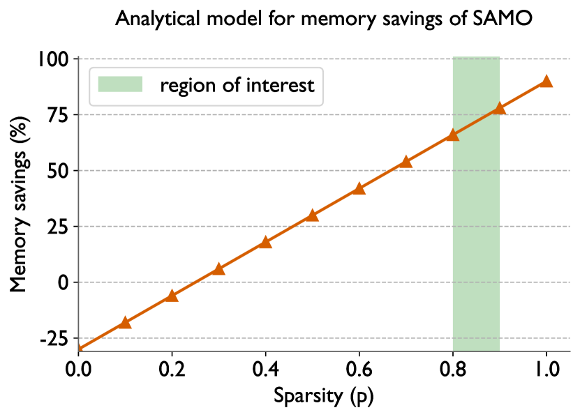
Figure 2: Percentage memory saved by SAMO as compared to default mixed-precision training. Sparsity here refers to the proportion of parameters that have been pruned. SAMO can save around 66-78% memory in a range of 0.8-0.9 sparsity, which is typical for most pruning algorithms in deep learning.

IV Exploiting SAMO for Improving Parallel Training Performance

When computing on a single GPU, SAMO simply reduces memory consumption with some overheads in the backward pass (compression of gradients) and the optimizer step (expansion of parameters). Hence, when training on a single GPU, SAMO does not lead to any performance improvements. This is because the total number of floating point operations in the forward and backward pass is unchanged (since we still compute in dense). In this section, we discuss how parameter pruning and SAMO can be used to optimize the performance of multi-GPU training.

The main performance bottleneck in parallel neural network training is communication. GPUs perform computation on data at a much faster rate than that of data communication between them on modern HPC interconnects. This problem is only exacerbated when training larger models, which require a correspondingly larger number of GPUs on a cluster. Thus, designing algorithms that can decrease the amount of communication can greatly benefit parallel deep learning. We now discuss how the application of SAMO on a pruned neural network can reduce communication in parallel training. As discussed in Section II, we use AxoNN, which implements a hybrid of inter-layer parallelism (point-to-point communication) and data parallelism (collective communication), to demonstrate the efficacy of our optimizations.

IV-A Optimizing collective communication in data parallelism

First, let us see how our optimizations can decrease the overhead of collective communication in the data parallel phase. After the end of the forward and backward pass, AxoNN synchronizes the local gradients of each GPU via an all-reduce. In Section III-A, we showed how SAMO stores the 16-bit gradients in a compressed format i.e. only for the unpruned parameters. This allows us to reduce the size of collective communication messages by directly invoking AxoNN’s all-reduce calls on the compressed tensor. This leads to a significant reduction in the collective communication time.

IV-B Optimizing point-to-point communication in inter-layer parallelism

As described in Section II, AxoNN implements a hybrid of inter-layer and data parallelism by dividing the work among $G_{\mathrm{inter}}\times G_{\mathrm{data}}$ GPUs. When SAMO is used to reduce the memory required for training a neural network, we can reduce the number of GPUs required to deploy a single instance of the neural network i.e. decrease $G_{\mathrm{inter}}$. This can allow us to use more GPUs for data parallelism, and increase $G_{\mathrm{data}}$. A reduced $G_{\mathrm{inter}}$ has the effect of decreasing the time spent in point-to-point communication thereby increasing the efficiency of inter-layer parallelism. We now provide a proof for this claim. We use the following notations:

• $B$ - Batch size

• $\mathrm{mbs}$ - The size of each microbatch

• $G$ - Number of GPUs

• $t_{f}$ - Time spent in computation on a microbatch of size $\mathrm{mbs}$ during the forward pass through the entire model

• $t_{b}$ - Time spent in computation on a microbatch of size $\mathrm{mbs}$ during the backward pass through the entire model

Note that $t_{f}$ and $t_{b}$ do not take the point-to-point communication cost into account. They just denote the compute time for the forward and backward pass across all the layers.

The time spent in point-to-point communication can be divided into two parts: the bubble time and the transmission time. A GPU experiences a pipeline bubble when there aren’t enough microbatches in the pipeline to keep all of the GPUs busy. As shown in Figure 3, different GPUs experience pipeline bubbles at different points in time. But a common theme is that pipeline bubbles occur towards the beginning and end of the computation of a batch. We define the transmission time as the total time spent in sending messages in the pipeline.

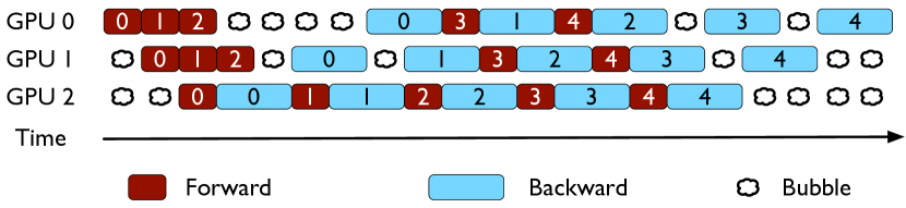
Figure 3: Illustration of how a batch is computed in inter-layer parallelism on three GPUs ($G_{\mathrm{inter}}=3$). In this example, we have divided the input batch into 5 microbatches (numbered 0 to 4). The red and blue colors denote forward and backward passes of microbatches respectively. We assume that the forward pass takes one unit of time and the backward pass takes two units of time. We observe that on each GPU, the pipeline bubble time accounts for 6 units, which equals the time to do $G_{\mathrm{inter}}-1=2$ forward passes and $G_{\mathrm{inter}}-1=2$ backward passes.

Let $t_{\mathrm{bubble}}$ and $t_{\mathrm{send}}$ denote the bubble time and transmission time respectively. Narayanan et al. [28] show that $t_{\mathrm{bubble}}$ equals the time it takes to complete forward and backward passes for $G_{\mathrm{inter}}-1$ microbatches on any GPU. We can also see this in Figure 3, wherein we observe that the bubble time for a pipeline with $G_{\mathrm{inter}}=3$ equals the time to do two forward and two backward passes. Assuming uniform distribution of compute, the time to complete the forward and backward pass of a microbatch on a single GPU is $\frac{t_{f}+t_{b}}{G_{\mathrm{inter}}}$.

Thus, the bubble time can be calculated as,

$$t_{\mathrm{bubble}} =(G_{\mathrm{inter}}-1)\times(\frac{t_{f}+t_{b}}{G_{\mathrm{inter}}})$$ (6)

$$=(t_{f}+t_{b})\times(1-\frac{1}{G_{\mathrm{inter}}})$$ (7)

Now, taking the derivative of $t_{\mathrm{bubble}}$ with $G_{\mathrm{inter}}$, we can show that the pipeline bubble time is a monotonically increasing function of $G_{\mathrm{inter}}$:

$$\frac{\partial t_{\mathrm{bubble}}}{\partial G_{\mathrm{inter}}} =\frac{t_{f}+t_{b}}{G^{2}_{\mathrm{inter}}}>0$$ (8)

Since SAMO can help in decreasing $G_{\mathrm{inter}}$ via its memory savings, we can conclude that it can be used to optimize the pipeline bubble time. Note that in Equation 8, we observe that the gradient w.r.t. $G_{\mathrm{inter}}$ is inversely proportional to its square. Thus, with a progressive increase in model size (which entails a corresponding increase in $G_{\mathrm{inter}}$), we expect diminishing returns in the bubble time improvement.

The transmission time $t_{\mathrm{send}}$ is proportional to the number of messages sent and received by each GPU. Each GPU sends and receives four messages per microbatch, two each in the forward and backward passes. Let us now derive the total number of microbatches each GPU computes on. First, AxoNN divides the input batch into $G_{\mathrm{data}}$ shards, one for each inter-layer parallel group. Next, each inter-layer parallel group breaks this batch shard into microbatches of size $\mathrm{mbs}$. These microbatches are processed by every GPU in the inter-layer parallel group. Thus the total number of microbatches computed upon by every GPU is $\frac{B}{G_{\mathrm{data}}\times\mathrm{mbs}}$. Thus, we can express $t_{\mathrm{send}}$ as,

$$t_{\mathrm{send}} \propto 4\times\frac{B}{\mathrm{mbs}\times G_{\mathrm{data}}}$$ (9)

$$\propto 4\times\frac{B}{\mathrm{mbs}}\times\frac{G_{\mathrm{inter}}}{G}(\because G_{\mathrm{inter}}\times G_{\mathrm{data}}=G)$$ (10)

Taking the derivative of Equation 10 w.r.t. $G_{\mathrm{inter}}$ shows that $t_{\mathrm{send}}$ is a monotonically increasing function of $G_{\mathrm{inter}}$:

$$\frac{\partial t_{\mathrm{send}}}{\partial G_{\mathrm{inter}}} \propto\frac{B}{\mathrm{mbs}\times G}>0$$ (11)

Hence, we can see that using SAMO to decrease $G_{\mathrm{inter}}$ can also help us decrease the transmission time for point-to-point communication in inter-layer parallelism. Thus, we have shown how the memory optimizations in SAMO can be exploited to reduce the collective communication pertaining to data parallelism and point-to-point communication pertaining to inter-layer parallelism respectively. Later, in Section VI, we provide performance profiles that demonstrate reduction in communication times as empirical evidence for the claims we have made in this section.

V Experimental Setup

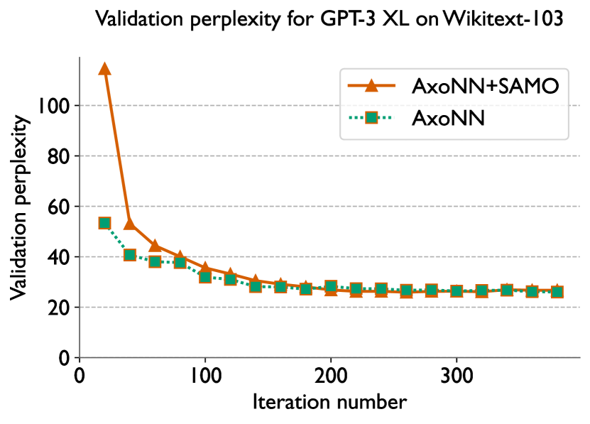
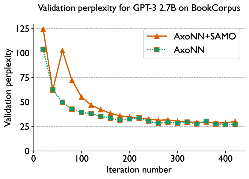
Figure 4: Validation perplexities for GPT-3 XL (left) and GPT-3 2.7B (right) on 64 and 128 GPUs of Summit respectively. For AxoNN+SAMO, we prune both models to a sparsity of 90% using [4]. We use the same hyperparameters as Brown et al. [2] and train on the Wikitext-103 [37] and BookCorpus datasets [38].

In this section, we provide details of the empirical experiments that we conducted to demonstrate the benefits of our optimizations. As discussed in Section II, we used AxoNN [13] for parallelizing the training process. We first validate the statistical efficiency of our implementation by training two neural networks to completion at a sparsity of 0.9. For pruning, we use You et al.’s “Early-Bird Tickets” pruning algorithm [4]. Then, we study the performance of two convolution neural networks (VGG-19 [39] and WideResnet-101 [40]) and four GPT-style transformer models from Brown et al. [2] under a strong scaling setup to demonstrate the hardware efficiency of our approach. We use the Oak Ridge National Laboratory’s Summit supercomputer to run our experiments. Summit has two POWER9 CPUs and six 16 GB NVIDIA V100 GPUs per node. Each CPU is connected to 3 GPUs via NVlink. The intra-node bandwidth, inter-node bandwidth, and the peak half-precision throughput are 50 GB/s, 12.5 GB/s and 125 Tflop/s per GPU respectively.

V-A Description of neural networks and hyperparameters

Table I lists the set of neural networks and the corresponding hyperparameters used in this study. VGG-19 [39] and WideResnet-101 [40] are two convolutional neural network (CNN) architectures widely used in computer vision. GPT-3 [2], a variant of the transformer architecture [41], is extremely popular in natural language processing for causal language modeling. For each model, we use the same hyperparameters (batch size, sequence length, learning rate schedules, gradient clipping, l2 regularization and optimizer hyperparameters) as used by the authors. We use SGD (with momentum [42]) and the AdamW [43] optimizer for training the CNN and GPT-3 models respectively. We use MegatronLM’s highly optimized kernels to implement the GPT-3 models [25]. For the convolution neural networks, we use implementations provided by the torchvision library.

TABLE I: List of neural networks used in this study. For each model, we list the minimum and maximum number of GPUs used in our strong scaling runs. We choose the minimum and maximum GPU counts such that the ratio of batch size to number of GPUs is 4 and 1 respectively.

Neural Network	# Parameters	Batch Size	No. of GPUs
WideResnet-101 [40]	126.89M	128	16–128
VGG-19 [39]	143.67M	128	16–128
GPT-3 XL [2]	1.3B	512	64–512
GPT-3 2.7B [2]	2.7B	512	64–512
GPT-3 6.7B [2]	6.7B	1024	128–1024
GPT-3 13B [2]	13B	2048	256–2048

We profile the neural networks listed in Table I under a strong scaling setup to demonstrate the efficacy of our optimizations. For every model, we choose the minimum and maximum GPU counts such that the ratio of batch size to number of GPUs is 4 and 1 respectively. For a given model, we fix the batch size irrespective of the GPU count. This is because while increasing the batch size leads to better performance, it also degrades the quality of convergence [44]. Under a strict definition of strong scaling, the final answer should be the same irrespective of the number of GPUs. Therefore, it is important to keep the global batch size fixed. For our approach, we prune the networks to a sparsity of 90% using You et al.’s “Early Bird Ticket” algorithm [4].

To ensure the correctness of our optimizations, we train GPT-3 XL and GPT-3 2.7B to completion on the Wikitext-103 dataset [37] and the BookCorpus dataset [38] respectively. We present the validation perplexity curves for AxoNN and AxoNN+SAMO. Again, we use a sparsity of 90% and the same pruning algorithm as the strong scaling runs. The purpose of this experiment to ensure that our proposed optimizations work correctly in an end-to-end fashion in combination with a pruning algorithm. Since this is a sanity check, the datasets we have used are much smaller than what are typically used to train large GPT-3 style language models. We highlight prior work by Samar et al. [45], who have successfully pruned GPT-3 style language models upto 90% on a much larger and challenging dataset (Pile [46].)

V-B Choice of frameworks

We integrate our optimizations in AxoNN [13] and refer to it as “AxoNN+SAMO”. We use AxoNN and DeepSpeed-3D [14, 29] as baselines for dense computations. DeepSpeed-3D implements a hybrid of data, inter-layer and intra-layer parallelism for parallel model training. Their data parallel implementation uses the ZeRO optimizer to shard optimizer state memory across data parallel ranks [29]. They use MegatronLM’s implementation of intra-layer parallelism of transformers [25]. DeepSpeed-3D has been used to train some of the largest neural networks till date such as Bloom-176B [34] and Megatron-Turing NLG 530B [35]. Finally, we integrate Sputnik  [11] in AxoNN to create a sparse matrix multiplication baseline. Note that Sputnik does not support sparse convolutions, so we do not implement the convolution architectures in Table I using Sputnik. We build our baselines using CUDA 11.0, PyTorch 1.12.0, NCCL 2.8.4, GCC 9.1.0 and Spectrum-MPI 10.4.0.3.

V-C Evaluation metrics

For the statistical efficiency experiments, we report perplexity on the validation split of the training dataset. Perplexity is defined as the exponential of the cross entropy loss. For our strong scaling runs, we report the average iteration time i.e. time to train on a single batch of input data. We do this by training for 100 batches and averaging the time of the last 90.

For the transformer models, we also calculate the percentage of peak half-precision flop/s. To do this, we use Narayanan et al.’s formula to derive the total number of floating point operations in a batch [28] of a transformer model and divide it by the average batch time over 100 training batches to derive the flop/s. Finally, we divide this quantity by 125 Tflop/s (the peak half-precision flops per GPU on Summit) and the number of GPUs to obtain the percentage of peak half-precision throughput.

Since Sputnik is a sparse matrix multiplication library, it only computes a fraction of the flops that the other dense computation frameworks compute. For instance at a sparsity of 90%, it would only compute 10% of the flops. For a fair comparison, we assume the same number of flops for Sputnik as the dense computation frameworks while using the time spent computing the sparse kernels.

VI Results

We now present the results of the empirical experiments outlined in Section V.

VI-A Statistical efficiency

We verify the statistical efficiency of AxoNN+SAMO by training GPT-3 XL [2] and GPT-3 2.7B [2] to completion at a sparsity of 90%. We use You et al.’s algorithm [4] to prune a neural network for AxoNN+SAMO. Figure 4 illustrates the results of this experiment. We observe that (1) the final validation perplexities for the pruned networks trained with AxoNN+SAMO match those of the unpruned network trained with AxoNN and (2) both AxoNN and AxoNN+SAMO reach the final validation perplexities in similar number of iterations. This verifies the correctness of our implementation.

VI-B Strong scaling performance

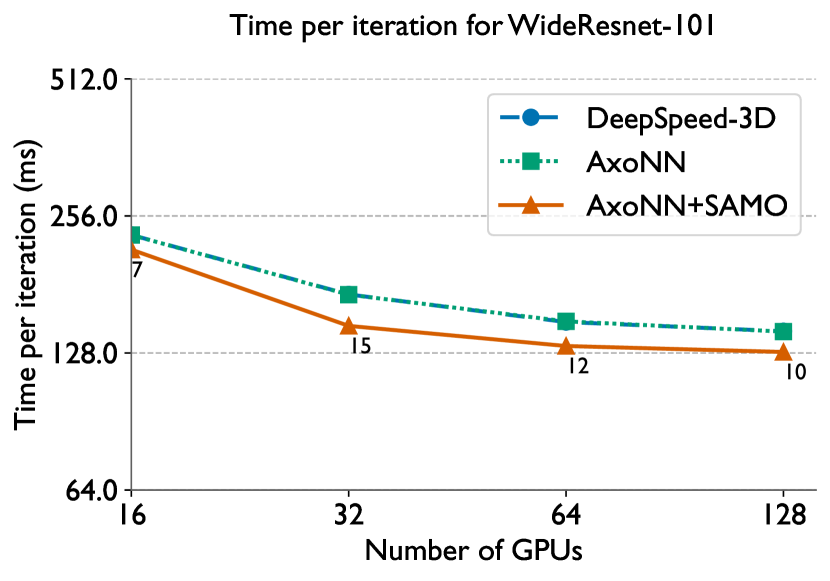
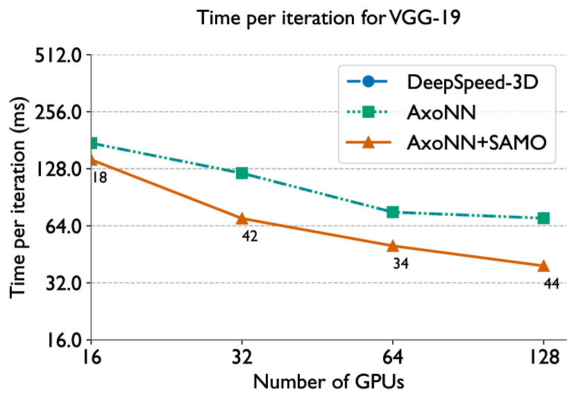
Figure 5: Time per iteration (batch time) for a strong scaling study of WideResnet-101 (left) and VGG-19 (right) on Summit. We prune the models to a sparsity of 90% for AxoNN+SAMO (see Table I for batch sizes). We annotate AxoNN+SAMO’s line with its percentage speedup over AxoNN.

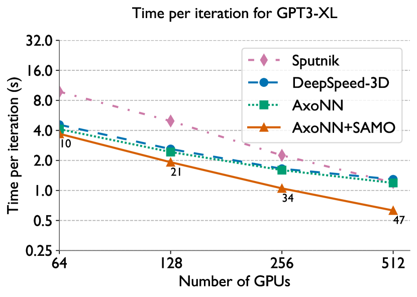
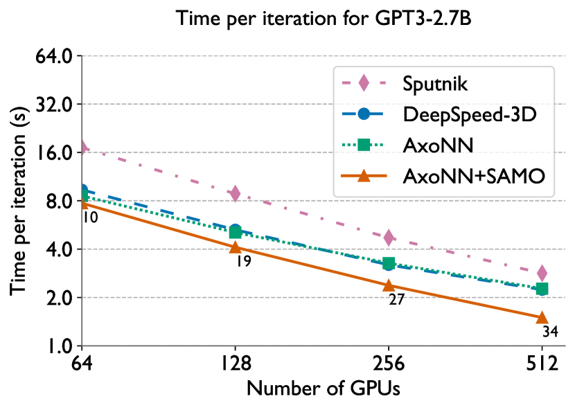
Figure 6: Time per iteration (batch time) for a strong scaling study of GPT-3 XL (left) and GPT-3 2.7B (right) on Summit. We prune the models to a sparsity of 90% for AxoNN+SAMO and Sputnik (see Table I for batch sizes). We annotate AxoNN+SAMO’s line with its percentage speedup over AxoNN.

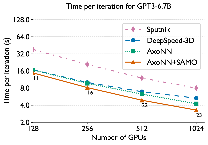
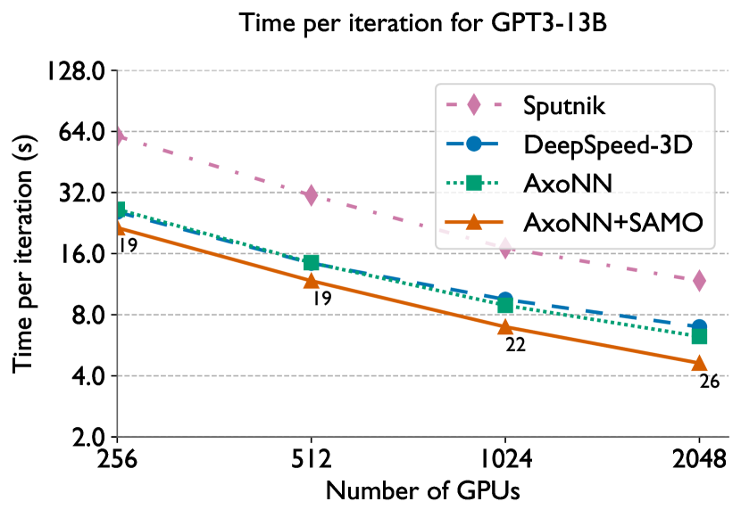
Figure 7: Time per iteration (batch time) for a strong scaling study of GPT-3 6.7B (left) and GPT-3 13B (right) on Summit. We prune the models to a sparsity of 90% for AxoNN+SAMO and Sputnik (see Table I for batch sizes). We annotate AxoNN+SAMO’s line with its percentage speedup over AxoNN.

Next, we illustrate the results of our strong scaling experiments on WideResnet-101 and VGG-19 in Figure 5, GPT-3 XL and GPT-3 2.7B in Figure 6, and on GPT-3 6.7B and GPT-3 13B in Figure 7. The CNNs used in this study are nearly 10–100$\times$ smaller than the GPT-3 based models (see Table I). Hence, all of AxoNN, DeepSpeed-3D and AxoNN+SAMO are able to run these architectures in a pure data parallel configuration, with a full copy of the network on each GPU. Thus the only communication here is the all-reduce on the network gradients. We illustrate these results in Figure 5. We observe similar batch times for both AxoNN and DeepSpeed-3D. This is explained by the fact that both these frameworks have very similar NCCL-based implementations of data parallelism. Our approach yields speedups of 7–12% over WideResnet-101 and 18–44% over VGG-19. While both these speedups are significant, SAMO seems to benefit the latter architecture more than the former. This is because the WideResnet-101 architecture spends nearly 1.5$\times$ more time in the computation phase as compared to VGG-19. Also, both these models have similar number of parameters and thus similar communication costs in the data-parallel all-reduce. Thus the proportion of the batch time spent by the WideResnet-101 architecture in communication is significantly smaller than VGG-19. Since our approach optimizes communication, the benefits for WideResnet-101 are smaller than that of VGG-19. Note that we do not run Sputnik for the CNNs as the library does not support sparse convolutions.

Let us now discuss the much larger GPT-3 based neural networks. These networks are too large to fit on a single GPU and are thus trained using hybrid parallelism. First, we observe that the performance of the sparse matrix computation library, Sputnik is significantly worse than both of our dense baselines – AxoNN and DeepSpeed-3D, as well as AxoNN+SAMO (Figures 6 and 7). This is in spite of the fact that the number of floating point operations computed by Sputnik is 10% of the other methods. This is in agreement with our observations in Figure 1 for fully connected layers on a single GPU. Thus, AxoNN+SAMO ends up being nearly twice as fast as Sputnik across all the GPT-3 style neural networks. It is evident from Figures 6 and 7 that augmenting AxoNN with our optimizations significantly improves its performance at scale. Our method speeds up the training of GPT-3 XL by 10–47%, GPT-3 2.7B by 10–24%, GPT-3 6.7B by 11–23% and GPT-3 13B by 19–26%. The speedups over DeepSpeed-3D are larger – 19–51%, 17–33%, 12–38% and 16.4–34% respectively for the four models.

We also present the percentage of peak half precision throughputs obtained for GPT-3 13B in Table II. We observe a significant reduction in the GPU utilization with increasing GPU counts for DeepSpeed-3D and AxoNN. This is a consequence of increasing communication to computation ratios. For both frameworks, the peak half precision throughput drops to around 20% at the largest profiled GPU counts. However, with AxoNN+SAMO, we observe a smaller reduction in hardware utilization, with a peak throughput of around 30% for the largest GPU count. This serves as empirical evidence of the fact that our optimizations indeed decrease the amount of communication in parallel training.

TABLE II: Percentage of peak half precision throughput for a strong scaling study of GPT-3 13B on Summit (see Table I for batch sizes). We prune the models to a sparsity of 90% for AxoNN+SAMO and Sputnik.

# GPUs	Sputnik	DeepSpeed-3D	AxoNN	AxoNN+SAMO
256	18.9	44.6	43.3	53.4
512	18.5	39.9	39.7	48.8
1024	16.8	30.1	32.2	41.1
2048	12.2	20.6	22.9	31.0

Since our optimizations are geared toward reducing the communication costs of training, we expect larger improvements over AxoNN as the number of GPUs increase. Again, this is because a larger proportion of time is spent in communication as we increase the scale of training. We find our observations in Figures 6 and 7 to be in agreement with this hypothesis. We indeed observe the largest speedups for the largest GPU counts, which are 47% and 34% for GPT-3 XL and GPT-3 2.7B on 512 GPUs, 23% for GPT-3 6.7B on 1024 GPUs, and 26% for GPT-3 13B on 2048 GPUs.

VI-C Performance Breakdowns

To verify that the speedups over AxoNN are indeed due to reduction in communication times, we profile the GPT-3 2.7B model on 128, 256 and 512 GPUs and provide breakdowns of the batch times in Figure 8. We divide the batch time into its non-overlapping phases, namely the compute (forward and backward pass), point-to-point communication, pipeline bubble (due to inter-layer parallelism), and collective communication (due to data parallelism). We use the CUDA Event API to profile the time spent in each of these phases.

At 128 GPUs, we observe that training is dominated by the point-to-point communication time. However as the number of GPUs increase, the proportion of time spent in the point-to-point communication also decreases. Note that this is in line with Equation 10, wherein we showed that the messaging time is inversely proportional to the number of GPUs.

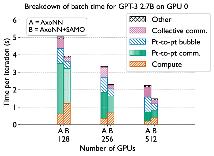
Figure 8: Breakdown of batch time for GPT-3 2.7B on Summit. We divide the batch time into its non-overlapping phases – computation, point-to-point communication, pipeline bubble (due to inter-layer parallelism), and collective communication (due to data parallelism). We use the CUDA Event API to profile the cumulative time spent in each of these phases.

We observe that the primary reason for AxoNN+SAMO’s improvement over AxoNN on 128 GPUs is due to a speedup in the point-to-point communication times. The absolute reduction in this time is 18% of AxoNN’s batch time. The improvements in the collective and pipeline bubble times account for 6% and 9% of AxoNN’s batch time. Thus for smaller GPU counts, we conclude that AxoNN+SAMO provides speedups primarily because of the improvements in the point-to-point communication times. The difference in the compute times is the overhead of compressing the parameter gradients at every backward pass (See Section III-C). The overhead accounts for 12% of AxoNN’s batch time and is significantly overcome by the 33% (18+6+9) improvement in the total communication time. We think that these overheads can be reduced by kernel level optimizations such as fusing the compression operation with the backward pass kernels. However, this is out of the scope of our current work.

At 256 GPUs, the point-to-point communication time is still dominant but not as much as 128 GPUs. In this case, the improvement in the point-to-point communication time accounts for a 16.17% of AxoNN’s batch time. As compared to 128 GPUs, the improvements in the bubble and collective communication times account for a significantly larger proportion of AxoNN’s batch time - 13.17% and 11.08%. The overhead in this case is 10.18% of the total batch time.

At 512 GPUs, we notice a very minor reduction in the point-to-point communication time. The reduction in the bubble and collective communication time account for 15% and 21% of AxoNN’s batch time respectively. The reduction in the point-to-point communication only improves the batch times by 4%. In this case, the overhead of compressing gradients is 8% of AxoNN’s batch time, which is again overcome by 40% (15+21+4) improvement in the total communication times.

VII Conclusion

It is well known that recent magnitude-based pruning approaches can lead to significant pruning of neural networks without reducing statistical efficiency [3, 4]. However, to the best of our knowledge, no prior work has attempted to exploit neural network pruning for improving the hardware efficiency of parallel neural network training. The primary deterrent to doing this is the sparse nature of the pruned subnetworks, which results in inefficient hardware performance.

In this work, we presented Sparsity-aware Memory Optimization (SAMO), a novel method that exploits the aforementioned parameter pruning algorithms to significantly reduce the memory consumption of neural network training while not sacrificing performance. We then demonstrated how these memory savings can be utilized to significantly improve the communication performance of two popular algorithms for parallel deep learning, data and inter-layer parallelism. We conducted strong scaling experiments on two convolution neural networks, and large GPT-style language models with 1.3 billion to 13 billion parameters proposed by Brown et al. [2] in their seminal work on the GPT-3 architecture. In our experiments, we consistently observed significant improvements over two highly scalable parallel deep learning frameworks – AxoNN and DeepSpeed-3D and a state-of-the-art sparse matrix computation library called Sputnik.

References

- [1] M. Belkin, D. Hsu, S. Ma, and S. Mandal, “Reconciling modern machine-learning practice and the classical bias-variance trade-off,” Proceedings of the National Academy of Sciences, vol. 116, no. 32, pp. 15 849–15 854, 2019. [Online]. Available: https://www.pnas.org/doi/abs/10.1073/pnas.1903070116
- [2] T. B. Brown, B. Mann, N. Ryder, M. Subbiah, J. Kaplan, P. Dhariwal, A. Neelakantan, P. Shyam, G. Sastry, A. Askell, S. Agarwal, A. Herbert-Voss, G. Krueger, T. Henighan, R. Child, A. Ramesh, D. M. Ziegler, J. Wu, C. Winter, C. Hesse, M. Chen, E. Sigler, M. Litwin, S. Gray, B. Chess, J. Clark, C. Berner, S. McCandlish, A. Radford, I. Sutskever, and D. Amodei, “Language models are few-shot learners,” CoRR, vol. abs/2005.14165, 2020. [Online]. Available: https://arxiv.org/abs/2005.14165
- [3] J. Frankle and M. Carbin, “The lottery ticket hypothesis: Finding sparse, trainable neural networks,” in International Conference on Learning Representations, 2019. [Online]. Available: https://openreview.net/forum?id=rJl-b3RcF7
- [4] H. You, C. Li, P. Xu, Y. Fu, Y. Wang, X. Chen, R. G. Baraniuk, Z. Wang, and Y. Lin, “Drawing early-bird tickets: Toward more efficient training of deep networks,” in International Conference on Learning Representations, 2020. [Online]. Available: https://openreview.net/forum?id=BJxsrgStvr
- [5] S. Prasanna, A. Rogers, and A. Rumshisky, “When BERT Plays the Lottery, All Tickets Are Winning,” in Proceedings of the 2020 Conference on Empirical Methods in Natural Language Processing (EMNLP). Online: Association for Computational Linguistics, Nov. 2020, pp. 3208–3229. [Online]. Available: https://aclanthology.org/2020.emnlp-main.259
- [6] Z. Liu, M. Sun, T. Zhou, G. Huang, and T. Darrell, “Rethinking the value of network pruning,” CoRR, vol. abs/1810.05270, 2018. [Online]. Available: http://arxiv.org/abs/1810.05270
- [7] C. Brix, P. Bahar, and H. Ney, “Successfully applying the stabilized lottery ticket hypothesis to the transformer architecture,” in Proceedings of the 58th Annual Meeting of the Association for Computational Linguistics. Online: Association for Computational Linguistics, Jul. 2020, pp. 3909–3915. [Online]. Available: https://aclanthology.org/2020.acl-main.360
- [8] J. Frankle, G. K. Dziugaite, D. R. 0001, and M. Carbin, “Linear mode connectivity and the lottery ticket hypothesis,” in Proceedings of the 37th International Conference on Machine Learning, ICML 2020, 13-18 July 2020, Virtual Event, ser. Proceedings of Machine Learning Research, vol. 119. PMLR, 2020, pp. 3259–3269. [Online]. Available: http://proceedings.mlr.press/v119/frankle20a.html
- [9] J. Maene, M. Li, and M.-F. Moens, “Towards understanding iterative magnitude pruning: Why lottery tickets win,” ArXiv, vol. abs/2106.06955, 2021.
- [10] C. Hong, A. Sukumaran-Rajam, I. Nisa, K. Singh, and P. Sadayappan, “Adaptive sparse tiling for sparse matrix multiplication,” in Proceedings of the 24th Symposium on Principles and Practice of Parallel Programming, ser. PPoPP ’19. New York, NY, USA: Association for Computing Machinery, 2019, p. 300–314. [Online]. Available: https://doi.org/10.1145/3293883.3295712
- [11] T. Gale, M. Zaharia, C. Young, and E. Elsen, “Sparse GPU kernels for deep learning,” in Proceedings of the International Conference for High Performance Computing, Networking, Storage and Analysis, SC 2020, 2020.
- [12] C. Yang, A. Buluc, and J. D. Owens, “Design principles for sparse matrix multiplication on the gpu,” 2018. [Online]. Available: https://arxiv.org/abs/1803.08601
- [13] S. Singh and A. Bhatele, “AxoNN: An asynchronous, message-driven parallel framework for extreme-scale deep learning,” in Proceedings of the IEEE International Parallel & Distributed Processing Symposium, ser. IPDPS ’22. IEEE Computer Society, May 2022.
- [14] Microsoft, “3d parallelism with megatronlm and zero redundancy optimizer,” https://github.com/microsoft/DeepSpeedExamples/tree/master/Megatron-LM-v1.1.5-3D_parallelism, 2021.
- [15] C. Liu, L. Zhu, and M. Belkin, “Toward a theory of optimization for over-parameterized systems of non-linear equations: the lessons of deep learning,” CoRR, vol. abs/2003.00307, 2020. [Online]. Available: https://arxiv.org/abs/2003.00307
- [16] S. S. Du, X. Zhai, B. Poczos, and A. Singh, “Gradient descent provably optimizes over-parameterized neural networks,” 2018. [Online]. Available: https://arxiv.org/abs/1810.02054
- [17] D. Soudry, E. Hoffer, M. S. Nacson, S. Gunasekar, and N. Srebro, “The implicit bias of gradient descent on separable data,” 2017. [Online]. Available: https://arxiv.org/abs/1710.10345
- [18] C. Zhang, S. Bengio, M. Hardt, B. Recht, and O. Vinyals, “Understanding deep learning requires rethinking generalization,” CoRR, vol. abs/1611.03530, 2016. [Online]. Available: http://arxiv.org/abs/1611.03530
- [19] A. Jacot, F. Gabriel, and C. Hongler, “Neural tangent kernel: Convergence and generalization in neural networks,” 2018. [Online]. Available: https://arxiv.org/abs/1806.07572
- [20] T. Gale, E. Elsen, and S. Hooker, “The state of sparsity in deep neural networks,” 2019. [Online]. Available: https://arxiv.org/abs/1902.09574
- [21] S. Gray, A. Radford, and D. P. Kingma, “Gpu kernels for block-sparse weights,” 2017. [Online]. Available: https://cdn.openai.com/blocksparse/blocksparsepaper.pdf
- [22] Z. Chen, Z. Qu, L. Liu, Y. Ding, and Y. Xie, “Efficient tensor core-based gpu kernels for structured sparsity under reduced precision,” in Proceedings of the International Conference for High Performance Computing, Networking, Storage and Analysis, ser. SC ’21. New York, NY, USA: Association for Computing Machinery, 2021. [Online]. Available: https://doi.org/10.1145/3458817.3476182
- [23] T. Dao, N. Sohoni, A. Gu, M. Eichhorn, A. Blonder, M. Leszczynski, A. Rudra, and C. Ré, “Kaleidoscope: An efficient, learnable representation for all structured linear maps,” in International Conference on Learning Representations, 2020. [Online]. Available: https://openreview.net/forum?id=BkgrBgSYDS
- [24] T. Dao, A. Gu, M. Eichhorn, A. Rudra, and C. Ré, “Learning fast algorithms for linear transforms using butterfly factorizations,” 2019. [Online]. Available: https://arxiv.org/abs/1903.05895
- [25] M. Shoeybi, M. Patwary, R. Puri, P. LeGresley, J. Casper, and B. Catanzaro, “Megatron-lm: Training multi-billion parameter language models using model parallelism,” 2020.
- [26] D. Narayanan, A. Harlap, A. Phanishayee, V. Seshadri, N. Devanur, G. Granger, P. Gibbons, and M. Zaharia, “Pipedream: Generalized pipeline parallelism for dnn training,” in ACM Symposium on Operating Systems Principles (SOSP 2019), October 2019. [Online]. Available: https://www.microsoft.com/en-us/research/publication/pipedream-generalized-pipeline-parallelism-for-dnn-training/
- [27] B. Yang, J. Zhang, J. Li, C. Re, C. Aberger, and C. De Sa, “Pipemare: Asynchronous pipeline parallel dnn training,” in Proceedings of Machine Learning and Systems, A. Smola, A. Dimakis, and I. Stoica, Eds., vol. 3, 2021, pp. 269–296. [Online]. Available: https://proceedings.mlsys.org/paper/2021/file/6c8349cc7260ae62e3b1396831a8398f-Paper.pdf
- [28] D. Narayanan, M. Shoeybi, J. Casper, P. LeGresley, M. Patwary, V. Korthikanti, D. Vainbrand, P. Kashinkunti, J. Bernauer, B. Catanzaro, A. Phanishayee, and M. Zaharia, “Efficient large-scale language model training on GPU clusters,” CoRR, vol. abs/2104.04473, 2021. [Online]. Available: https://arxiv.org/abs/2104.04473
- [29] S. Rajbhandari, J. Rasley, O. Ruwase, and Y. He, “Zero: Memory optimizations toward training trillion parameter models,” in Proceedings of the International Conference for High Performance Computing, Networking, Storage and Analysis, ser. SC ’20. IEEE Press, 2020.
- [30] S. Rajbhandari, O. Ruwase, J. Rasley, S. Smith, and Y. He, “Zero-infinity: Breaking the gpu memory wall for extreme scale deep learning,” ser. SC ’21. New York, NY, USA: Association for Computing Machinery, 2021. [Online]. Available: https://doi.org/10.1145/3458817.3476205
- [31] T. Ben-Nun and T. Hoefler, “Demystifying parallel and distributed deep learning: An in-depth concurrency analysis,” ACM Comput. Surv., vol. 52, no. 4, Aug. 2019. [Online]. Available: https://doi.org/10.1145/3320060
- [32] P. Micikevicius, S. Narang, J. Alben, G. Diamos, E. Elsen, D. Garcia, B. Ginsburg, M. Houston, O. Kuchaiev, G. Venkatesh, and H. Wu, “Mixed precision training,” in International Conference on Learning Representations, 2018. [Online]. Available: https://openreview.net/forum?id=r1gs9JgRZ
- [33] T. Chen, B. Xu, C. Zhang, and C. Guestrin, “Training deep nets with sublinear memory cost,” 2016.
- [34] BigScience, “Bigscience large open-science open-access multilingual language model,” https://huggingface.co/bigscience/bloom, 2022.
- [35] S. Smith, M. Patwary, B. Norick, P. LeGresley, S. Rajbhandari, J. Casper, Z. Liu, S. Prabhumoye, G. Zerveas, V. Korthikanti, E. Zhang, R. Child, R. Y. Aminabadi, J. Bernauer, X. Song, M. Shoeybi, Y. He, M. Houston, S. Tiwary, and B. Catanzaro, “Using deepspeed and megatron to train megatron-turing nlg 530b, a large-scale generative language model,” 2022. [Online]. Available: https://arxiv.org/abs/2201.11990
- [36] D. P. Kingma and J. Ba, “Adam: A method for stochastic optimization,” in 3rd International Conference on Learning Representations, ICLR 2015, San Diego, CA, USA, May 7-9, 2015, Conference Track Proceedings, Y. Bengio and Y. LeCun, Eds., 2015. [Online]. Available: http://arxiv.org/abs/1412.6980
- [37] S. Merity, C. Xiong, J. Bradbury, and R. Socher, “Pointer sentinel mixture models,” CoRR, vol. abs/1609.07843, 2016. [Online]. Available: http://arxiv.org/abs/1609.07843
- [38] Y. Zhu, R. Kiros, R. Zemel, R. Salakhutdinov, R. Urtasun, A. Torralba, and S. Fidler, “Aligning books and movies: Towards story-like visual explanations by watching movies and reading books,” in arXiv preprint arXiv:1506.06724, 2015.
- [39] K. Simonyan and A. Zisserman, “Very deep convolutional networks for large-scale image recognition,” in 3rd International Conference on Learning Representations, ICLR 2015, San Diego, CA, USA, May 7-9, 2015, Conference Track Proceedings, Y. Bengio and Y. LeCun, Eds., 2015. [Online]. Available: http://arxiv.org/abs/1409.1556
- [40] S. Zagoruyko and N. Komodakis, “Wide residual networks,” 2016. [Online]. Available: https://arxiv.org/abs/1605.07146
- [41] A. Vaswani, N. Shazeer, N. Parmar, J. Uszkoreit, L. Jones, A. N. Gomez, Ł. Kaiser, and I. Polosukhin, “Attention is all you need,” in Advances in neural information processing systems, 2017, pp. 5998–6008.
- [42] N. Qian, “On the momentum term in gradient descent learning algorithms,” Neural Networks, vol. 12, no. 1, pp. 145–151, 1999. [Online]. Available: https://www.sciencedirect.com/science/article/pii/S0893608098001166
- [43] I. Loshchilov and F. Hutter, “Fixing weight decay regularization in adam,” CoRR, vol. abs/1711.05101, 2017. [Online]. Available: http://arxiv.org/abs/1711.05101
- [44] N. S. Keskar, D. Mudigere, J. Nocedal, M. Smelyanskiy, and P. T. P. Tang, “On large-batch training for deep learning: Generalization gap and sharp minima,” in International Conference on Learning Representations, 2017. [Online]. Available: https://openreview.net/forum?id=H1oyRlYgg
- [45] Cerebras-AI, “Creating sparse gpt-3 models with iterative pruning,” https://www.cerebras.net/blog/creating-sparse-gpt-3-models-with-iterative-pruning, 2022.
- [46] L. Gao, S. Biderman, S. Black, L. Golding, T. Hoppe, C. Foster, J. Phang, H. He, A. Thite, N. Nabeshima, S. Presser, and C. Leahy, “The pile: An 800gb dataset of diverse text for language modeling,” CoRR, vol. abs/2101.00027, 2021. [Online]. Available: https://arxiv.org/abs/2101.00027