Searching for Gravitational-Wave Counterparts using the Transiting Exoplanet Survey Satellite

Abstract

In 2017, the LIGO and Virgo gravitational wave (GW) detectors, in conjunction with electromagnetic (EM) astronomers, observed the first GW multi-messenger astrophysical event, the binary neutron star (BNS) merger GW170817. This marked the beginning of a new era in multi-messenger astrophysics. To discover further GW multi-messenger events, we explore the synergies between the Transiting Exoplanet Survey Satellite (TESS) and GW observations triggered by the LIGO-Virgo-KAGRA Collaboration (LVK) detector network. TESS’s extremely wide field of view of $\sim$2300 deg² means that it could overlap with large swaths of GW localizations, which can often span hundreds of deg² or more. In this work, we use a recently developed transient detection pipeline to search TESS data collected during the LVK’s third observing run, O3, for any EM counterparts. We find no obvious counterparts brighter than about 17th magnitude in the TESS bandpass. Additionally, we present end-to-end simulations of BNS mergers, including their detection in GWs and simulations of light curves, to identify TESS’s kilonova discovery potential for the LVK’s next observing run (O4). In the most optimistic case, TESS will observe up to one GW-found BNS merger counterpart per year. However, TESS may also find up to five kilonovae which did not trigger the LVK network, emphasizing that EM-triggered GW searches may play a key role in future kilonova detections. We also discuss how TESS can help place limits on EM emission from binary black hole mergers, and rapidly exclude large sky areas for poorly localized GW events.

1 Introduction

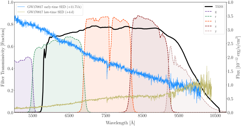
Figure 1: The TESS band (black line) compared to the optical and near-infrared bands of Pan-STARRS (Tonry et al., 2012) (dotted lines). These have been plotted alongside the early-time (light blue) and late-time (tan) spectral energy distributions (SEDs) of the optical counterpart to GW170817 (Shappee et al., 2017). The SED of the kilonova becomes redder as time passes, showing that TESS’s bandpass is uniquely positioned to continuously observe the decay of the afterglow over a timescale of days.

In 2017 August, the LIGO (Aasi et al., 2015) and Virgo (Acernese et al., 2014) gravitational-wave (GW) observatories detected the binary neutron star (BNS) merger GW170817 (Abbott et al., 2017a), which was coincident with the Fermi Gamma Ray Space Telescope’s detection of GRB170817A (Goldstein et al., 2017). This event ushered in the age of GW multi-messenger astronomy, with detections of the resulting kilonova and afterglow in the X-ray, UV, optical, infrared, and radio (Abbott et al., 2017b; Ciolfi, 2020, and references therein). The LVK’s last observing run, O3, brought the total number of detected GW events to 90. Only one of the events detected during O3 had a potential EM counterpart (Graham et al., 2020); no EM counterparts were detected for any other events (Abbott et al., 2021a).

The next observing run for the LVK, O4, is expected to begin in 2023. With significantly upgraded sensitivity and an expanded detector network (with the addition of KAGRA (Akutsu et al., 2021; Aso et al., 2013; Somiya, 2012)), O4 promises to bring many more GW detections. EM counterparts will be searched for across the spectrum by many facilities, including but not limited to optical surveys such as the Zwicky Transient Facility (ZTF; Anand et al. 2020a), the Asteroid Terrestrial-impact Last Alert System (ATLAS; Tonry et al. 2018), and the All-Sky Automated Search for Supernovae (ASAS-SN; de Jaeger et al. 2021); targeted infrared searches such as the Wide-Field Infrared Transient Explorer (WINTER; Frostig et al. 2022); wide-field radio follow-up from the Murchison Wide-Field Array (MWA; Kaplan et al. 2016) and other observatories (see, e.g, Dobie et al. 2019; Callister et al. 2019); as well as rapid X-ray and gamma-ray follow-up from the Neil Gehrels Swift Observatory and the Fermi Space Telescope (Oates et al., 2021; Tohuvavohu et al., 2020; Fletcher et al., 2021).

In this paper, we suggest that another space-based observatory, the Transiting Exoplanet Survey Satellite (TESS), is poised to play a useful role in EM follow-up of GW detections. TESS was launched in 2018 April and has been conducting an all-sky survey since 2018 July, with the primary goal of finding transiting exoplanets around M-dwarfs (Ricker et al., 2015). TESS’s four cameras cover $\sim$2300 deg² on the sky, observing the same region (a “sector”) continuously for $\sim 27$ days. As of 2023 February, it has observed $\sim$ sixty sectors, covering approximately 90% of the entire sky. In the context of GW follow-up, we highlight TESS’s enormous field-of-view (FOV) and extensive periods of uninterrupted observation. The TESS bandpass spans from 600-1000 nm; see Fig. 1 for a visual representation of the TESS band compared to the set of passbands used in the Panoramic Survey Telescope and Rapid Response System (Pan-STARRS; Chambers et al. 2016). TESS’s broad wavelength coverage spans nearly the entirety of the Pan-STARRS $r$, $i$, $z$, and $y$ passbands; we also show the evolution of the SED of GW170817 (Shappee et al., 2017). The SED reddens over a timescale of days, but remains in TESS’s passband throughout.

TESS’s Prime Mission (from 2018 July to 2020 July) was successful, with over 2 000 “Objects of Interest” (i.e., planet candidates) detected (Guerrero et al., 2021). Data from TESS, in conjunction with recently-developed software, including the TESS-reduce difference imaging pipeline (Ridden-Harper et al., 2021), have also contributed significantly to transient science. Key scientific results include population-level studies of Type Ia supernovae (Fausnaugh et al., 2021a), constraints on the progenitor properties of the double-peaked Type IIb supernova SN2021zby (Wang et al., 2022), characterization of the optical afterglow of the gamma-ray burst GRB191016A (Smith et al., 2021), analyses of early-time light curves of tidal disruption events (Holoien et al., 2019) and core-collapse supernovae (Vallely et al., 2021), and identification of periodic active galactic nucleus (AGN) outbursts (Payne et al., 2021).

TESS’s Extended Mission 2 (EM2), which began in 2022 September, brought with it configuration changes that will prove beneficial to the rapid detection and follow-up of transients. The two main changes in EM2 are the reduced integration time for each full-frame image (FFI) (200 s) and the increased frequency of data downlinks to Earth (weekly instead of biweekly). Additionally, during EM2, FFIs will be more frequently released after they have been processed using the TESS Image CAlibrator (tica; Fausnaugh et al. 2020). These factors, in conjunction with our pipeline to identify transients in TESS FFIs (described briefly in Section 2.2.1), will allow for the rapid identification and follow-up of transient candidates, including kilonovae.

In Sec. 2, we present our results from a search of TESS FFI data concurrent with the LVK’s O3 to establish preliminary limits on any EM counterparts to BNS, neutron star–black hole (NSBH), and binary black hole (BBH) mergers whose GW localizations coincided with TESS’s FOV. We then discuss in Sec. 3 the results of a simulation for the LVK’s next observing run, O4, and TESS’s prospects for observing kilonovae. We estimate the number of kilonovae detectable in TESS via both GW-triggered searches of the data and blind searches of the TESS data. Finally, in Sec. 4, we discuss the implications of our results, additional applications of TESS for GW follow-up, and the niche that TESS will occupy in the growing field of multi-messenger astronomy.

2 TESS observations of O3 events

The LVK’s third observing run (O3), which spanned from 2019 April to 2020 March, resulted in a combined 75 GW events. Of these, 39 were released as part of the 2nd Gravitational-wave Transient Catalog (GWTC-2; Abbott et al. 2021b), and 35 were part of GWTC-3 (Abbott et al., 2021a). One other event, GW200105_162426—a marginal NSBH candidate—was released separately (Abbott et al., 2021c). The events were also released on the Gravitational Wave Open Science Center (GWOSC; Abbott et al. 2021d). 69 detections from O3 were confident BBH mergers, three were consistent with NSBH mergers, and one was a BNS merger. Two events had masses which fell in the “lower mass gap” (Shao, 2022), indicating that they could either be NSBH or BBH mergers.

Significant EM follow-up campaigns ensued from the publicly released GW events during O3. In particular, the BNS and NSBH mergers mentioned above attracted considerable attention from optical and near-infrared observers. A slew of observatories searched for potential counterparts to these mergers, including ZTF (Coughlin et al., 2020; Anand et al., 2020a; Graham et al., 2022), SAGUARO (Paterson et al., 2021; Lundquist et al., 2019), SkyMapper (Chang et al., 2021), ASAS-SN (de Jaeger et al., 2021), DECam (Anand et al., 2020b; Andreoni et al., 2019), GRANDMA (Antier et al., 2020), GOTO (Gompertz et al., 2020), GECKO (Kim et al., 2021), and J-GEM (Sasada et al., 2021). See Appendix A of Abbott et al. (2021a) and references therein for details and information on observations in other EM domains. Besides the AGN flare ZTF19abanrhr which Graham et al. theorize to have resulted from an AGN accretion disk disrupted by the BBH merger GW190521 (Abbott et al., 2020d), no EM counterparts were found by any search.

O3 temporally overlapped with TESS sectors 10 through 23 (the first two LVK observing runs, O1 and O2, occurred before TESS’s launch). Sectors 10–13 were located in the southern ecliptic hemisphere, while Sectors 14–23 were located in the North. Each sector was observed for two orbits of 13–14 days each, with a day-long gap during the data downlinks between each orbit. During these sectors, TESS captured FFIs of its entire FOV with an integration time of 30 minutes. An estimate for the 3-$\sigma$ limiting magnitude of a single 30 min FFI, for sectors with low backgrounds, is 19.11 in the TESS band (see, e.g., Fausnaugh et al. 2019). By stacking these FFIs on timescales of 8 hours or longer, we can probe fainter magnitudes, down to 21–22; a more thorough discussion of such a technique is presented in Rice & Laughlin (2020).

In this section, we conduct a GW-triggered search of the TESS FFIs for each event in GWTC-3 to search for optical and near-infrared counterparts to BNS, NSBH, and BBH mergers. Searching for counterparts to such events will allow us to establish limits on the types of emission we may expect to observe from future events during O4. For instance, while BNS mergers at sufficiently close distances (such as GW170817) are expected to produce detectable kilonovae, we may also observe an electromagnetic counterpart for certain NSBH mergers with favorable masses and spins (Zhu et al., 2021; Biscoveanu et al., 2022; Foucart, 2020). On the other hand, EM emission from BBH events is usually not expected (Doctor et al., 2019).

Our search for potential EM counterparts in TESS FFIs consists of two parts. First, we find overlaps between a GW probability skymap and the concurrent TESS sector, as well as the TESS sectors spanning until 40 days post-GW trigger. Then, for skymaps in which $>1\%$ of the overall probability is enclosed in the TESS field of view for either a simultaneous or subsequent sector, we search through TESS FFIs for candidate transient events using our pipeline (Jayaraman et al. in prep). Here, we provide a high-level overview of this pipeline; full details are beyond the scope of this work and will be discussed in a separate paper.

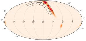
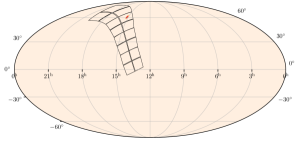
Figure 2: Examples of TESS coverage of GW skymaps, plotted in celestial coordinates, for two individual gravitational-wave events. Left: The best TESS-covered event in O3, the BBH merger GW200209_085452, which was concurrent with TESS sector 21. The enclosed probability is 0.719. No EM counterparts were found in a search of TESS data. Right: An example simulated BNS event for O4, where the entire probability is enclosed in the concurrent TESS sector 50. This event’s associated simulated light curve peaks at 19.4 mag in the TESS band, which is easily detectable in TESS with an 8-hour stack of FFIs (this 8-hour stack pushes the 3-$\sigma$ detection limit to $\sim$21). For an event such as this, the entire GW localization region would be observed in the TESS FOV, meaning that TESS would be able to supply not only a precise localization, but also photometry showing the full rise and evolution of the kilonova light curve.

2.1 Skymap overlap calculation

To assess the utility of TESS in identifying a potential EM counterpart for a given GW event, we developed a tool that constructs and calculates the overlap between a given TESS sector and a GW probability skymap. For each of the 16 TESS CCDs, the tool constructs a polygon, accounting for the gaps between the cameras and CCDs. To translate from detector coordinates to sky coordinates, we use the World Coordinate System (WCS) data in the FFI file headers for existing data (Greisen & Calabretta, 2002; Calabretta & Greisen, 2002). For future sectors, we use models from planned pointings (presented in Kunimoto et al. 2022, and also available on the TESS website). Each pixel in the GW probability skymap is checked to determine if it falls into a TESS CCD’s FOV, and the total probability enclosed in TESS is then integrated. See Fig. 2 for two examples of the overlap between a GW event and the TESS FOV: one from GW200209_085452, a BBH event from O3, and another from a BNS simulated for O4.

Often, the selected TESS sector will be the one concurrent with the GW observation; however, overlap integrals can also be calculated for any other sector. For example, while TESS’s duty cycle is extremely high (at $\sim$90%), TESS undergoes a data downlink or is otherwise observationally disrupted approximately 10% of the time. Telemetry interruptions are predictable and can be accounted for. Sometimes, however, TESS data collected during nominal operations can be unusable. A fraction of FFIs from every sector (ranging from $\lesssim 10$% to $\gtrsim 40$%) suffer from elevated backgrounds due to scattered light from the Earth and the Moon when they are above the spacecraft sunshield. Scattered light levels in each sector can be qualitatively predicted based on properties of the TESS orbit, and we can adjust our search strategy accordingly. The lowest sky backgrounds occur in sectors that occur between December and March. All relevant information regarding the TESS data (formats, disruptions, scattered light, etc.) is documented in the corresponding Data Release Notes.

For events in portions of the data affected by instrument issues or suffering from significant amounts of scattered light, we can calculate the overlap with the next available sector to identify any afterglows or other similar emission. Another reason to calculate the overlap with subsequent sector(s) is that some models of EM emission from binary mergers predict somewhat delayed emission; for instance, Equation 3 in Graham et al. (2020) suggests that EM emission from BBH mergers can occur tens of days after the coalescence. Thus, if a GW trigger occurs at the end of a sector, it would be prudent to search for evidence of an EM counterpart throughout the subsequent one to two sector(s), a timespan of $\sim$ 50 days. While we understand that these timescales remain poorly constrained, we adopt this strategy to serve as a proof-of-concept in our initial search of archival TESS data.

2.2 Searches in Archival Data

For each of the 75 events from O3 in GWTC-2 and -3, we construct and calculate the overlap with the TESS FOV for the concurrent and subsequent sectors, up to $\sim 50$ days after the trigger (an example plot is shown in the left panel of Figure 2). Then, we selected GW events where $>1$% of the probability was enclosed within the TESS field of view of the concurrent or subsequent sector(s); this reduced the number of events we analyzed to 50. Of these, 33 had $>1$% of the probability enclosed in the concurrent sector, while 17 had that amount of probability enclosed in a subsequent sector. Both cases were treated identically, in terms of the search technique. The distribution of skymap probability enclosed in TESS for the 75 BNS, NSBH, and BBH events found in GWs in O3 is shown in Fig. 3.

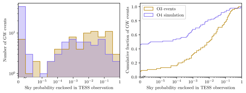
Figure 3: Histogram (left) and cumulative distribution (right) of GW skymap probability enclosed in TESS for O3 events and for the O4 BNS simulation. The O3 distribution includes all 75 events (BBH, NSBH, and BNS) publicly released by the LVK as part of GWTC-2 and -3. If the GW event happened while TESS was not observing (7 of the 75 events), the overlap integral was calculated for the next available set of observations. The O4 distribution is for the 96 simulated BNS events. Because the simulated O4 events tend to have smaller GW localization areas due to the improved GW sensitivity and enlarged detector network, the chance of TESS observing part of the skymap is reduced compared to the O3 events. This is most evident in the cumulative distribution, where the fraction of O4 simulated events for which none of the skymap is covered by TESS is more than double that of the O3 events. At the other end of the distribution, where almost all of the skymap probability is covered by TESS, the gap between the O3 events and the O4 simulation narrows. This is because well-localized events have more concentrated areas of probability; either they are mostly covered by TESS or not at all.

2.2.1 Transient Identification

In order to identify transient candidates that could correspond to an EM counterpart to the GW trigger, we used a pipeline developed specifically to find transients in TESS FFIs (Jayaraman et al. in prep). This pipeline produces difference images using the ISIS package (Alard & Lupton, 1998) based on a median image constructed from $\sim$ 20 individual FFIs with low backgrounds. It calculates a root-mean-square (RMS) image from these, then finds strongly time-varying sources in this image using Source Extractor (Bertin & Arnouts, 1996). These sources are matched against the Gaia eDR3 catalog (Gaia Collaboration et al., 2016, 2021) and discarded if they are brighter than 19.5 in the G_RP band and have a parallax that is not consistent with zero (as that would likely correspond to a known stellar source). We then filter the remaining sources through a convolutional neural network which has been trained on cutouts from the RMS images of TESS transients that were discovered by other observatories and surveys during prior sectors. This network assigns a probability for each source that captures its likelihood of being a bona fide transient. The pipeline constructs light curves for sources that have been assigned a probability greater than 0.6. This results in a set of $\mathcal{O}(\gtrsim 1000)$ light curves per sector. The remaining light curves are still too many for a human to review in order to triage them for follow-up, so we make use of a light curve clustering algorithm that uses a random forest and the HDBSCAN algorithm (Campello et al., 2013) to identify anomalous light curves that could correspond to transients. Clusters of light curves correspond to typical variability patterns, such as stellar variability (pulsations and eclipses) from nearby stars, scattered light patterns, and instrumental effects inherent to the CCD, such as hot pixels. We review these final light curves by eye and study the most promising candidates in further detail. An analysis of the non-kilonova transients detected by our pipeline and a more rigorous estimate of its limits will be discussed in a forthcoming paper.

2.2.2 O3 search results

GW skymaps are composed of HEALPix (Górski et al., 2005; Zonca et al., 2019) pixels, which have limited resolution compared to TESS. TESS pixels are 21” on a side, while the highest resolution pixels in GW skymaps average 52” on a side, or $\sim 2.5$ TESS pixels (this corresponds to a value of 4096 for the HEALPix NSIDE parameter), but most have significantly lower resolutions. We use the ang2pix function in healpy to match each TESS transient to its corresponding GW HEALPix skymap pixel.

We extracted $\lesssim 500$ possible light curve matches per GW event for most of the considered events. For some events, we found over 1000 matching TESS transient triggers. However, the vast majority of these are false positives, due to subtraction artifacts and nearby variable stars. We discarded light curves corresponding to (a) instrumental noise (high RMS scatter or discontinuities in flux measurements), (b) long-period variability associated with any rotation or pulsation in a known nearby variable star (within $<$ 35”), or (c) consistency with the flux signature of a cataclysmic variable outburst (these targets were cross-referenced with existing CV catalogs, such as that in Drake et al. 2014). Additionally, we discarded light curves that matched faint stars in Gaia EDR3. After the visual examination, we identified 76 (of the total $\sim$ 10 000) light curves associated with GW event skymaps that were not filtered based on the above criteria. These 76 light curves had rises in flux starting $\sim$10–20 days after the associated GW event, with rises spanning tens of days.

We investigated these rises in flux to ensure that they were not merely instrumental effects or contamination from nearby variable stars. To evaluate the possibility of instrumental systematics, we examined a 7 px $\times$ 7 px cutout from the raw FFI around the source in question; single-pixel effects are strongly localized, and do not appear in nearby pixels in these images. We also plotted all sources from Gaia EDR3 within 3 arcmin of each detected source; if there was a bright star (G${}_{\rm RP}\lesssim$ 13.5) within 2 TESS pixels whose signal clearly bled into the central pixel of the cutout, that candidate source was discarded. After filtering based on these criteria, we were left with 17 candidates that merited further investigation.

We then searched existing catalogs using the NASA/IPAC Extragalactic Database—including the WISE point source catalog (Cutri & et al., 2012), GALEX point source catalog (Bianchi et al., 2017), and the SDSS galaxy catalog (Ahumada et al., 2020). We also queried the Pan-STARRS1 image cutout server and point source catalog from the MAST database (Chambers et al., 2016) to determine whether there was a galaxy at that location. Eight of the the 17 remaining light curves corresponded to WISE or GALEX point sources; these, along with the remaining nine sources, were ruled out as candidates due to the presence of a faint Gaia star (G_RP dimmer than 13.5) in each of the 40” $\times$ 40” Pan-STARRS cutouts around the coordinates of the light curves. To further verify all the cases in which we suspected contamination from Gaia stars in the vicinity, we downloaded the available FFI light curves for these stars from MAST and plotted them using the lightkurve package (Lightkurve Collaboration et al., 2018). These light curves were identical in morphology to the sources from the pipeline, demonstrating that the light curves found arise from contamination.

Our pipeline was thus unable to identify any EM counterparts to BBH mergers in the region of the GW skymaps that overlaps the TESS FOV. There is no detection of any obvious counterpart in the TESS FOV peaking above 17th magnitude in the TESS band. However, work is ongoing to more fully characterize the performance and detection limits of our transient pipeline, including deeper searches with lengthier stacks such as those presented in the light curve simulation section (Sec. 3.2.1) below. Our work represents one of the first attempts to conduct a “blind” search for transients fainter than 17th magnitude in TESS. Prior work in this arena (Tingay & Yang, 2019) centered on a specific goal—to identify optical counterparts to fast radio bursts in TESS’s FOV. Tingay & Yang established a non-detection limit at 16th magnitude. However, by broadening this search to all classes of transients (including counterparts to compact object mergers), TESS can cast a wider net and possibly answer lingering questions about transient physics across a wide range of transient events.

We paid particular attention to the events which included at least one neutron star and thus are more likely to result in EM emission: the BNS GW190425, the confident NSBHs GW191219_163120, GW200105_162426, and GW200115_042309, and the potential NSBHs GW190814 and GW200210_092254. Counterparts from these events such as kilonovae are expected to peak within 1–2 days of the GW trigger, so we focused on the TESS sectors that were concurrent with the GW merger time. Unfortunately, TESS did not overlap significantly with the skymaps for these events, with the most considerable overlap being 3.9% of the sky probability for the NSBH GW191219_163120 during sector 19. The NSBH events represented 12 of the 76 light curves that were flagged during our visual inspection. Further analysis of these light curves did not reveal anything consistent with kilonova light curves. One event, GW200210_092254, did have a light curve associated with its localization that had a rise and fall during the TESS observation. However, the start of emission occurs $\sim$ 15 days after the GW trigger, much longer than what most kilonova models predict. Additionally, the coordinates of the EM transient lie at the 99.8% credible level of the GW localization area, indicating that it is highly unlikely to be associated with GW200210_092254. Thus, we claim no kilonova detections from the overlapping region of TESS’s FOV and the GW skymaps from O3, down to at least a limiting magnitude of $\sim$ 17. Future work may strengthen these constraints.

2.2.3 SDSS J1249+3449

In addition to the “blind” search for EM transients from O3 (discussed above), we also studied the TESS light curve of the quasar SDSS J124942.30+344928.9. Graham et al. argued that a flare observed in this galaxy (referred to as J1249) in 2019 June might correspond to a BBH merger product being kicked upward through the accretion disk of an AGN. TESS observed J1249 in Sectors 22 (2020 Feb–March) and 49 (2022 Feb–March).

We extracted light curves at the position of J1249 from the TESS FFIs using forced photometry, as described in Fausnaugh et al. (2021b). The results are shown in Figure 4. After correcting for measurement uncertainties (Nandra et al., 1997; Vaughan et al., 2003), the light curve from Sector 22 is consistent with a constant light curve on timescales longer than 8 hours. For Sector 49, the light curve is flat but exhibits a residual scatter of 5.8% on 8 hour timescales after correcting for measurement uncertainties. On shorter timescales than 8 hours, there is formally more observed variability than can be explained with statistical uncertainties at the 2% level. However, inspection of the difference images shows that the variability is not associated with the AGN and so is likely due to residual systematic errors or a nearby variable star. These systematic errors likely contribute to the excess variance at 8 hour timescales.

The Sector 49 observations were approximately three years after the original flare in 2019 and so are consistent with the expected timescale for the re-entry of the BBH merger remnant into the AGN disk. However, the short TESS baseline of 27 days is poorly suited to identify flares lasting 50 days or longer, especially considering uncertainties in the delay between the merger event and ejection of the remnant from the disk (Graham et al., 2022), as well as uncertainty in the orbital period of the remnant. We therefore cannot put a meaningful constraint the BBH merger hypothesis for J1249 with these TESS observations.

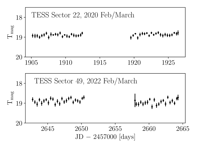
Figure 4: TESS light curves of SDSS J1249+3449, the AGN with a flare reported by Graham et al.. The light curves are binned to 8 hours, and the error bars show the standard deviation in each bin scaled by the square-root of the number of data points. In Sector 22, the light curve is consistent with a constant light curve. In Sector 49, there is excess variability at the 5% level, but inspection of the difference images suggests that these are residual systematic errors.

3 Simulated performance in O4

During the LVK’s next observing run, O4, the increased sensitivity of GW detectors and the addition of KAGRA to the overall detector network will mean that GW events are expected multiple times per week, and potentially even daily (Abbott et al., 2020b). The majority of these events will be BBH mergers, with a comparatively smaller number of BNS and NSBH mergers (Abbott et al., 2020c). In this section, we evaluate the prospects of detecting a kilonova in TESS.

3.1 Simulated BNS population and light curves

To simulate a population of kilonovae in O4, we use the BNS simulations released in Frostig et al. (2022), which include 625 neutron star mergers with realistic mass and spin distributions. In these simulations, BNS mergers are placed uniformly in comoving volume out to a luminosity distance ($d_{L}$) of 400 Mpc and isotropically positioned on the sky, and are distributed randomly in time over the 2022 calendar year.

Each event is then associated with a GW detector configuration, assuming a duty cycle of 70% (i.e., each detector has a 70% chance of being in observing mode) and added into Gaussian noise. The PyCBC Live matched-filter GW search algorithm is then used to recover each BNS using detector power spectral densities (PSDs) representative of O4 sensitivities (Nitz et al., 2018; Dal Canton et al., 2020; Abbott et al., 2020a). We consider an event to be detected in GWs if PyCBC Live recovers it with a network signal-to-noise ratio (S/N) greater than 9. Each detected event is also associated with a localization from the full bilby parameter estimation pipeline (Ashton et al., 2019; Romero-Shaw et al., 2020); see Frostig et al. (2022) for further details on the simulation.

In our analysis, we choose astrophysical BNS merger rates of 50, 250, and 1000 Gpc^-3 yr^-1; these represent a broad range that spans the current uncertainties from various population models presented in LIGO–Virgo–KAGRA Collaboration (2021). For each rate, we calculate the total number of mergers with $d_{L}<400$ Mpc in one year (e.g., 52 events for the 250 Gpc^-3 yr^-1 rate). We then randomly draw with replacement that number of events from the set of 625. Each event is associated with a light curve and a determination of whether or not it is detected in GWs. This process is repeated 100 times, each with a different random seed, for each rate to build a distribution of possible results for O4.

For each of the 625 events, we generate simulated kilonovae light curves using the Kasen et al. (2017) models for the TESS bandpass. These models are computed by solving for relativistic radiation transport in radioactive plasma, with the assumption of a spherical kilonova geometry. The models have three parameters: the mass of the dynamical ejecta $M_{\rm{ej}}$, the expansion velocity of that ejecta $v_{\rm{ej}}$, and the lanthanide fraction of the ejecta $X_{\rm{lan}}$. We use fitting formulae from Coughlin et al. (2019) to determine $M_{\rm{ej}}$ and $v_{\rm{ej}}$ from the primary and secondary masses ($m_{1}$ and $m_{2}$) simulated for each event. The lanthanide fraction $X_{\rm{lan}}$ remains a free parameter; since $X_{\rm{lan}}$ for binary neutron star mergers remains poorly understood, we choose four values of $X_{\rm{lan}}$ to generate light curves: $10^{-2}$, $10^{-3}$, $10^{-4}$, and $10^{-5}$.

We then run the overlap tool described in Sec. 2.1 for the GW bilby skymaps corresponding to each of the events found in gravitational waves. Figure 3 shows the distribution of TESS-enclosed probabilities for the simulated O4 BNS events. The distribution is roughly similar to the distribution of detected BBH, NSBH, and BNS events from O3, with slightly less probability enclosed for the simulated O4 events due to the improved localizations compared to O3 (and therefore more reliant on serendipitous observation for any significant coverage).

3.2 Simulation results

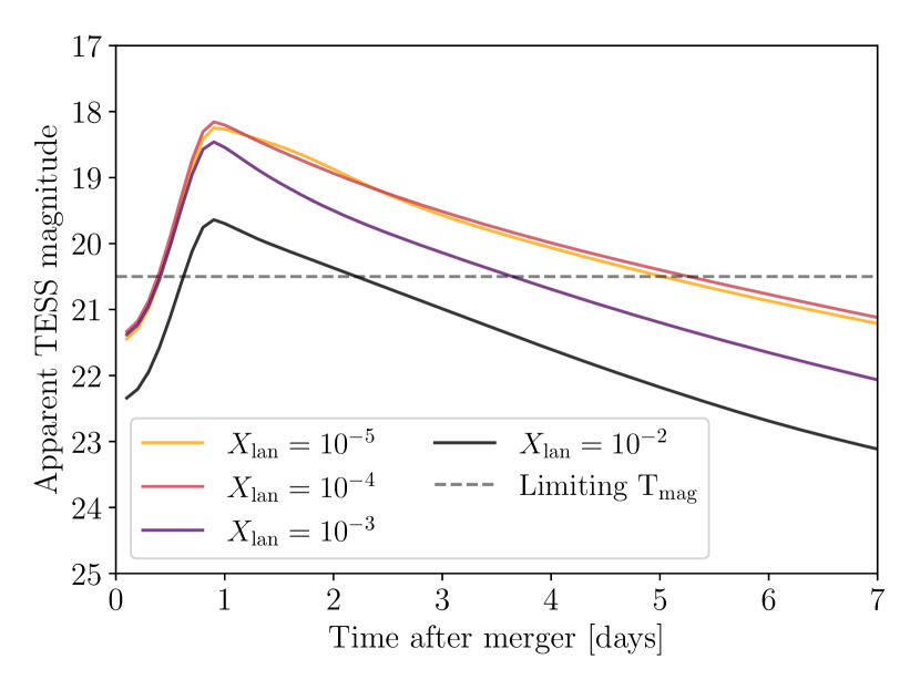
Figure 5: Example TESS-band kilonova light curves for one of the brightest GW-detected events in the simulation, for a BNS merger at a luminosity distance of 64 Mpc. Light curves for various values of the lanthanide fraction ($X_{\rm lan}$) are shown, along with an estimate for the 3-$\sigma$ TESS limiting magnitude of a 4-hour stack ($T_{\rm mag}\sim 20.5$). Ejecta with higher lanthanide fractions have lower opacity, which obscures the optical and near-infrared emission. Since the TESS bandpass is in the optical and near-infrared, it is more sensitive to kilonovae with lower lanthanide fractions. For all lanthanide fractions, TESS should be able to observe at least part of the rise and decay of the light curve of a sufficiently bright kilonova.

3.2.1 Light curves

In Figure 5, we show results for the simulated light curves in the TESS band across various lanthanide fractions, for one of the brightest GW-detected events in the simulation. We find that the lowest lanthanide fractions $X_{\rm{lan}}$ of $10^{-4}$ and $10^{-5}$ lead to very similar light curves, which are the brightest in the TESS band. The $X_{\rm{lan}}=10^{-3}$ curve is slightly less luminous by $\sim 0.25$ mag at its peak; this difference increases to nearly one full magnitude in the tail of the light curve. The $X_{\rm{lan}}=10^{-2}$ light curve is significantly dimmer: it peaks about two magnitudes lower than the $X_{\rm{lan}}=10^{-5}$ and $X_{\rm lan}=10^{-4}$ models. These results are caused by the large number of line transitions for lanthanides which lead to high opacities (Kasen et al., 2013). This opacity acts to obscure optical emission at higher lanthanide fractions, resulting in relatively stronger infrared emission. While TESS’s passband does receive some infrared signal (it is broad-band from 600 to 1000 nm; see Fig. 1), the bulk of its passband is in the optical and near-infrared. This makes it comparatively better suited for observations of kilonovae with lower lanthanide fractions. GW170817, which Waxman et al. (2018) suggest had $X_{\rm lan}\sim 10^{-3}$ (corresponding to the purple light curve in Figure 5), would have been detected by TESS had it been observing that region of sky.

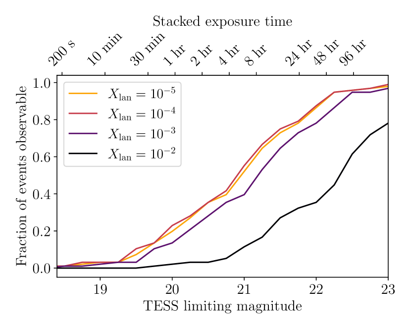
Figure 6: Distribution of the fraction of GW-detected events observable as a function of the overall stacked integration time and (top axis) and TESS limiting magnitude (bottom axis), at a variety of lanthanide fractions. Stacking TESS FFIs lowers the limiting magnitude, allowing us to detect more events, especially for kilonovae with lower lanthanide fractions. For higher lanthanide fractions (e.g., $X_{\rm{lan}}=10^{-2}$), over three-quarters of events will not be detectable at an 8 hour stack ($\sim$ 21 mag); the majority would require an FFI stack of a day or more to be detectable. Lower lanthanide fractions, on the other hand, will result in almost 60% of GW-detected events being bright enough to be detectable using an $\sim$8 hour stack of FFIs. Note that the limiting magnitude as a function of stacked exposure time presented here is based only on counting noise on the source and background. In practice, the limiting magnitude can vary significantly, by up to 2-3 magnitudes, due to image backgrounds, proximity of targets to other bright objects, and other factors.

We note that TESS’s limiting magnitude, and thus its sensitivity to kilonovae, is closely related to the timescale at which the light curve is binned. During TESS’s EM2, the stacked integration time of each FFI will be 200 seconds; consequently, stacking the FFIs (or, similarly, binning the resulting light curves) will likely be necessary to reveal faint transients. Figure 6 shows the fraction of events observable as a function of TESS limiting magnitude and stacked exposure time. The mapping between stacked exposure time and limiting magnitude was done based on (a) the counting uncertainty in background-dominated FFIs being 0.409 e^-/s (assuming an aperture of 4 pixels) and (b) the zeropoint of TESS being 20.44 (i.e., this is the magnitude corresponding to a count rate of 1 e^-/s).

If BNS ejecta have lanthanide fractions as high as $X_{\rm{lan}}=10^{-2}$, stacking FFIs to 8 hours (reaching a limit of $\sim$21 mag) will reveal less than 20% of BNS mergers found in GWs. At lower lanthanide fractions, almost half of BNS mergers in the TESS FOV will be bright enough to be detectable with an 8-hour stack; with a 24-hour stack, nearly all such mergers are detectable.

However, when we stack images or bin light curves, we experience a tradeoff between limiting magnitude and the number of useful data points. For instance, stacking FFIs over many days can push limiting magnitudes down to 21.5 (or even slightly fainter—Rice & Laughlin 2020, for example, reach 21.8), but will only provide one data point every few days with which to identify kilonovae. Since kilonovae rise and fade on the order of days, this can make discerning kilonovae at fainter magnitudes more difficult, if not impossible. These binned light curves could also be confused with other, non-kilonova signals; consequently, it is crucial to carefully choose the stacking or binning timescale to reach fainter magnitudes while not washing out any useful signal. A minimum stacked integration time of 30 min (i.e., stacking 9 200-s FFIs to a limiting magnitude of 19.6) is necessary to detect any substantial fraction of kilonovae. For shorter stacks, only a few percent of GW-found BNS mergers result in EM emission that will be detectable in TESS. These estimates are also all under the optimistic expectation that the backgrounds in the light curves are low; in certain sectors, scattered light can cause high backgrounds in the FFIs. In those cases these detection limits would become brighter, closer to 19th magnitude for an 8-hour stack (see, e.g., Fausnaugh et al. 2021a).

Figure 7 shows light curves in the TESS band for all 96 BNS events out of the 625 simulated events which were detected in GWs, assuming an $X_{\rm{lan}}=10^{-5}$. The median light curve peaks at just fainter than 21 mag, with the brightest 5% peaking between 18 and 19 mag. The light curves tend to fade at a similar rate of 0.5 mag/day regardless of the values of the ejecta mass $M_{\rm ej}$ and velocity $v_{\rm ej}$. This suggests that the vast majority of kilonova detections in TESS will be aided by stacking FFIs and/or binning light curves to probe these sources that are at the limit of TESS’s sensitivity.

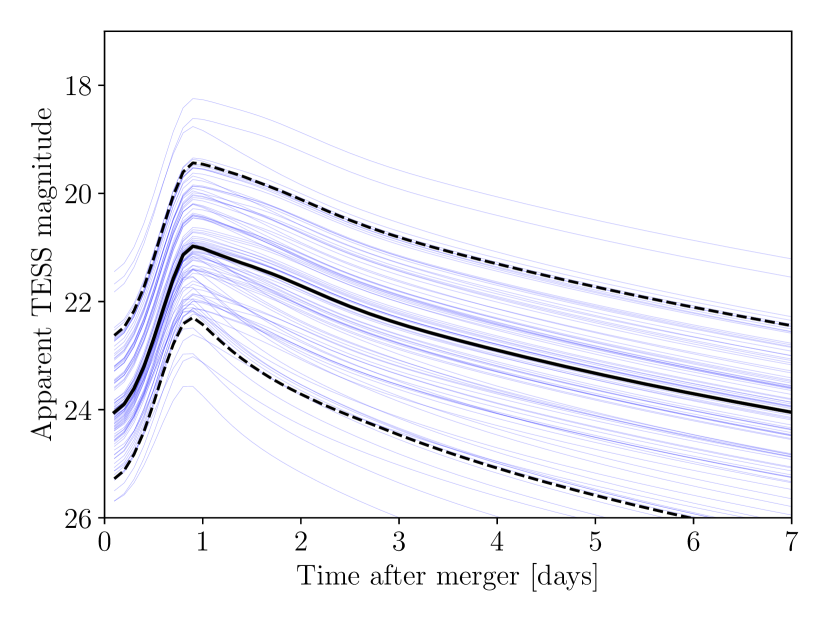
Figure 7: TESS-band light curves for all 96 simulated O4 BNS events found in gravitational waves for $X_{\rm{lan}}=10^{-5}$. Individual light curves are shown in light blue. The median light curve is in solid black, and the 90% interval is bounded by the black dotted lines. The brightest light curves can peak at almost 18 mag, whereas the median light curve peaks near 21 mag. Despite varying dynamical ejecta mass $M_{\rm{ej}}$ and ejecta expansion velocity $v_{\rm{ej}}$ across the simulated events, the light curves tend to all peak at $\sim 1$ day after merger and subsequently decay at a similar rate.

3.2.2 Events in TESS

Next, events detected by PyCBC Live in gravitational waves are checked to see if they are within the TESS FOV. The number of BNSs identified in gravitational waves over a year of observations during O4 ranges from a mean of 1.5 for the most pessimistic rate to 32 at the most optimistic (90% confidence interval), where we have averaged over our 100 random seeds. While we cannot establish a single limit for detectability in TESS due to the variable backgrounds in different sectors, we can evaluate the number of kilonovae detected at various limiting magnitudes. These limiting magnitudes, as discussed above, correspond to different stacking times for the FFIs. Table 1 gives the number of events detected in GWs, covered by the TESS FOV, and bright enough to be detectable by TESS for each merger rate at various limiting magnitudes.

Table 1: Results for BNS mergers found in gravitational waves. We present the astrophysical BNS rate, the number of events found in gravitational waves by a matched-filtering search, the number of events which are in the TESS FOV, and of those, the number of events which have simulated TESS light curves brighter than a limiting magnitude of 21. These light curves assume a $X_{\rm{lan}}=10^{-5}$. In this simulation, using reasonable stacked integration times to probe deeper than a limiting magnitude of 21 does not result in any change in the number of observable kilonovae. For the “Found,” “Covered,” and “Bright” columns, we report the mean over 100 random seeds, as well as the median, 5th, and 95th percentiles in parentheses.

BNS rate	Found	Covered	Bright at
(Gpc-3yr-1)	in GWs	by TESS	limiting mag 21
50	1.5 ($1^{+2}_{-1}$)	0 ($0^{+0}_{-0}$)	0 ($0^{+0}_{-0}$)
250	8.5 ($8^{+5}_{-3}$)	0.2 ($0^{+1}_{-0}$)	0.1 ($0^{+1}_{-0}$)
1000	33 ($33^{+9}_{-7}$)	0.7 ($0^{+3}_{-0}$)	0.4 ($0^{+2}_{-0}$)

These results for the number of events covered in TESS are in line with a simple order of magnitude calculation: both the detected BNS events and the TESS coverage during EM2 are roughly isotropic across the sky, and TESS at any given observation covers $\sim$5.6$\%$ of the sky. Taking the median value of the most optimistic rate (32 events in GWs), multiplied by this percentage, results in 1.8 events covered in the TESS FOV; this value is within the uncertainty of the value found in the simulation (mean of 0.4, with median and 5th, 95th percentiles of $0^{+3}_{-0}$).

Figure 3 shows the distribution of probability enclosed by TESS for the 96 BNS events simulated and found in GWs. The simulated performance at enclosed probabilities larger than 10% is similar to that of the 75 BNS, NSBH, and BBH mergers observed in O3, with approximately 25% of events having greater than 5% of their probability enclosed in TESS.

3.3 Subthreshold simulation results

Table 2: Results for subthreshold BNS mergers not found in gravitational waves. Same as in Table 1, but for subthreshold events which are below the GW search algorithm’s signal-to-noise ratio threshold and thus deemed to not be found in gravitational waves. Here, we also show results for various limiting magnitudes which can be obtained with stacked integration times.

BNS rate	Found	Covered	Bright at limiting mag
(Gpc-3yr-1)	in GWs	by TESS	21.5	21	20.5
50	0	0.6 ($0^{+2}_{-0}$)	0.2 ($0^{+1}_{-0}$)	0.2 ($0^{+1}_{-0}$)	0.1 ($0^{+1}_{-0}$)
250	0	2.7 ($3^{+2}_{-3}$)	1.1 ($1^{+2}_{-1}$)	0.7 ($1^{+1}_{-1}$)	0.6 ($0^{+2}_{-0}$)
1000	0	11.0 ($11^{+5}_{-4}$)	4.6 ($5^{+3}_{-4}$)	3.0 ($3^{+3}_{-3}$)	2.2 ($2^{+3}_{-2}$)

Thus far, we have discussed searching TESS data with a GW-triggered search. TESS’s wide FOV and continuous observation capabilities mean that it can also be used to conduct a search for BNSs in the opposite direction, with potential kilonovae in TESS triggering subsequent searches in GW data, similar to searches performed in ZTF (Andreoni et al., 2021). Unlike ground-based surveys, TESS enjoys uninterrupted coverage that spans for weeks, with no periods of night; its pointing stability ($\lesssim 1\%$ of a pixel for a 1-hour stack) is also such that stacking TESS FFIs is more straightforward than stacking ground-based images. These properties mean that TESS is particularly well suited to searching for fast and faint transients such as kilonovae that may require significant stacking to achieve a confident detection. As a proof of concept, we repeat the analysis in Sec. 3.2.2 for “subthreshold” events, which were below the PyCBC Live S/N threshold and thus not detected in GWs. These results are presented in Table 2.

Even for the lowest BNS rate, we find that TESS could potentially identify one kilonova independent of GW observations. For the highest rate, we expect to observe means of between two and five BNS events, depending on the stacked integration time. This emphasizes the importance of EM-triggered searches in GW data, which trawl deeper into GW detector noise. Additional compact object mergers are statistically guaranteed to exist in the GW data at lower S/N, and joint searches between the LVK detector network and TESS will contribute towards recovering them.

4 Discussion

The results presented in Sec. 3 assume a TESS detection if the kilonova light curve peaks above the limiting magnitude for a given stack of FFIs (e.g., for a 4-hour stack, the limiting magnitude is 20.5). This simplification is reasonable in the mode where a search is being conducted in TESS, based on a pre-existing GW trigger with a skymap and a time. On the other hand, searches in TESS for subthreshold GW events will necessarily be shallower, and multiple data points above the limiting magnitude will be needed to definitively classify a light curve as a signature of the EM emission arising from a compact object merger. This assumption means that our subthreshold search results presented here are likely optimistic. However, they still represent an important new synergistic use of TESS with GW detectors in the LVK network, and a kilonova discovery using TESS—independent of LVK—would be significant.

In our analysis, we have also focused largely on the results for $X_{\rm{lan}}=10^{-5}$, which typically lead to the brightest light curves in the mostly-optical TESS band. Lower values of $X_{\rm{lan}}$ will likely lead to worse kilonova performance from TESS. Waxman et al. (2018) provides an estimate of $X_{\rm lan}\sim 10^{-3}$ for GW170817. However, they also note that this is a poorly constrained value, as there remain significant uncertainties in the values of the infrared opacities of heavy elements such as the lanthanides and their relative contributions to the opacity of kilonova ejecta (see, e.g., Kasen et al. 2013).

Despite these caveats and the small number of expected detections in O4, TESS remains a powerful tool for multi-messenger astronomy, especially since these observations have no opportunity cost compared to other targeted follow-up programs. TESS’s observing schedule is set well in advance, and unlike targeted follow-up, there are no targets that must be prioritized over others. Furthermore, the potential treasure trove of TESS FFIs are publicly released on a weekly basis without any proprietary period, which makes them particularly useful for transient searches and follow-up.

If another GW170817-like event occurs in O4 and happens to be in TESS’s FOV, the kilonova should be bright enough that TESS will catch the rise of the light curve. GW170817 peaked at about 17.5 mag in the i- and z-bands (Drout et al., 2017), which have overlap with the TESS bandpass (see Fig. 1). Crucially, we will obtain a light curve from TESS with a data point every 200 s. The kilonova signal for such an event may be visible in the raw light curve already, but stacking the FFIs to probe fainter magnitudes and using these stacks to construct a binned light curve may help us identify further trends in the light curve’s rise. TESS will join the ranks of new surveys such as BlackGEM (Bloemen et al., 2016), the Argus Array (Law et al., 2022), and others (Chase et al., 2021) in performing high-cadence, wide-field imaging of potential GW counterparts. These surveys can help constrain kilonova physics.

Finally, we can take advantage of TESS’s wide FOV to exclude large areas of the skymap to preserve telescope time for other observers. Since TESS’s observing and downlink schedules are known well in advance and processing times are consistent, we will be able to say at the moment of a GW event whether or not TESS was concurrently observing any part of the probability skymap. If so, we can expedite the processing of the data after downlink and focus our search on the highest-likelihood regions of the overlap using our transient pipeline. This, along with possible integration into the TreasureMap online service (Wyatt et al., 2020), can help other observatories with smaller FOVs plan their observing schedules to avoid redundancy with TESS. This will likely increase the chance of detecting a kilonova (or other EM counterpart) before it fades away forever.

5 Conclusion

We have conducted an analysis of TESS’s capabilities for observations of EM counterparts to GW events, with a study of archival TESS data from O3 and a simulation for TESS’s performance and potential contributions for kilonovae observations during O4, slated to begin in 2023 March. We find no evidence of EM counterparts in TESS during O3 down to a magnitude of $\sim 17$ after inspection of all skymaps with more than 1% sky probability that overlapped with the TESS FOV. We also find no evidence for a re-entry flare from the AGN that Graham et al. report as the site of an potential EM counterpart to the BBH merger GW190521, during the two sectors that TESS observed it.

In O4, with the most optimistic BNS rate of 1000 Gpc^-3yr^-1 and a favorable $X_{\rm{lan}}$ of $10^{-5}$, we expect at most one detection in TESS of a BNS merger found in GWs; however, lower rates and/or larger lanthanide fractions may lower this detection rate and make a concrete kilonova identification more unlikely. On the other hand, we find that GW-independent searches in TESS for kilonovae may be able to uncover up to five “subthreshold” BNS events which are buried in GW detector noise (for the most optimistic BNS rate), highlighting the utility of EM-triggered searches in GW data.

Finally, we discuss other aspects of TESS and its capabilities which make it a powerful tool for multimessenger astronomy. Chief among these is that searches in TESS data do not require any additional planning or telescope time, as its observations of specific regions of the sky are made on a fixed schedule set years in advance. Consequently, there is no tradeoff necessary between multi-messenger science and other observational interests, unlike other targeted follow-up programs for EM counterparts to GW events. Additionally, its wide FOV and continuous month-long observations make it one of the most ideal observatories for serendipitous observations of transients which might be missed by traditional ground-based surveys; besides the GW events mentioned here, neutrinos and gamma ray bursts may also prove to be complementary targets. We expect TESS’s EM2 and LVK’s O4 to produce a treasure trove of data and observations that could significantly enhance our understanding of compact object mergers.

References

- Aasi et al. (2015) Aasi, J., Abbott, B. P., Abbott, R., et al. 2015, Class. Quant. Grav., 32, 074001. http://dx.doi.org/10.1088/0264-9381/32/7/074001
- Abbott et al. (2017a) Abbott, B., Abbott, R., Abbott, T., et al. 2017a, Physical Review Letters, 119, doi:10.1103/physrevlett.119.161101. http://dx.doi.org/10.1103/PhysRevLett.119.161101
- Abbott et al. (2020a) Abbott, B. P., Abbott, R., Abbott, T. D., & et al. 2020a, Noise curves used for Simulations in the update of the Observing Scenarios Paper, https://dcc.ligo.org/LIGO-T2000012/public, ,
- Abbott et al. (2017b) Abbott, B. P., Abbott, R., Abbott, T. D., et al. 2017b, The Astrophysical Journal, 848, L12. http://dx.doi.org/10.3847/2041-8213/aa91c9
- Abbott et al. (2020b) —. 2020b, Living Reviews in Relativity, 23, doi:10.1007/s41114-020-00026-9. http://dx.doi.org/10.1007/s41114-020-00026-9
- Abbott et al. (2020c) —. 2020c, Living Rev. Rel., 23, 3. http://dx.doi.org/10.1007/s41114-020-00026-9
- Abbott et al. (2020d) Abbott, R., et al. 2020d, Phys. Rev. Lett., 125, 101102
- Abbott et al. (2021a) —. 2021a, arXiv:2111.03606
- Abbott et al. (2021b) Abbott, R., Abbott, T., Abraham, S., et al. 2021b, Physical Review X, 11, doi:10.1103/physrevx.11.021053. http://dx.doi.org/10.1103/PhysRevX.11.021053
- Abbott et al. (2021c) Abbott, R., Abbott, T. D., Abraham, S., et al. 2021c, The Astrophysical Journal Letters, 915, L5. http://dx.doi.org/10.3847/2041-8213/ac082e
- Abbott et al. (2021d) Abbott, R., et al. 2021d, SoftwareX, 13, 100658
- Acernese et al. (2014) Acernese, F., Agathos, M., Agatsuma, K., et al. 2014, Classical and Quantum Gravity, 32, 024001. http://dx.doi.org/10.1088/0264-9381/32/2/024001
- Ahumada et al. (2020) Ahumada, R., Prieto, C. A., Almeida, A., et al. 2020, ApJS, 249, 3
- Akutsu et al. (2021) Akutsu, T., et al. 2021, PTEP, 2021, 05A102
- Alard & Lupton (1998) Alard, C., & Lupton, R. H. 1998, ApJ, 503, 325
- Anand et al. (2020a) Anand, S., Coughlin, M. W., Kasliwal, M. M., et al. 2020a, Nature Astronomy, 5, 46–53. http://dx.doi.org/10.1038/s41550-020-1183-3
- Anand et al. (2020b) Anand, S., et al. 2020b
- Andreoni et al. (2019) Andreoni, I., et al. 2019, Astrophys. J. Lett., 881, L16
- Andreoni et al. (2021) —. 2021, Astrophys. J., 918, 63
- Antier et al. (2020) Antier, S., Agayeva, S., Almualla, M., et al. 2020, Monthly Notices of the Royal Astronomical Society, 497, 5518–5539. http://dx.doi.org/10.1093/mnras/staa1846
- Ashton et al. (2019) Ashton, G., Hübner, M., Lasky, P. D., et al. 2019, The Astrophysical Journal Supplement Series, 241, 27. http://dx.doi.org/10.3847/1538-4365/ab06fc
- Aso et al. (2013) Aso, Y., Michimura, Y., Somiya, K., et al. 2013, Phys. Rev. D, 88, 043007
- Bertin & Arnouts (1996) Bertin, E., & Arnouts, S. 1996, A&AS, 117, 393
- Bianchi et al. (2017) Bianchi, L., Shiao, B., & Thilker, D. 2017, ApJS, 230, 24
- Biscoveanu et al. (2022) Biscoveanu, S., Landry, P., & Vitale, S. 2022, arXiv:2207.01568
- Bloemen et al. (2016) Bloemen, S., et al. 2016, Proc. SPIE Int. Soc. Opt. Eng., 9906, 990664
- Burke et al. (2020) Burke, C. J., Levine, A., Fausnaugh, M., et al. 2020, TESS-Point: High precision TESS pointing tool, Astrophysics Source Code Library, , , ascl:2003.001
- Calabretta & Greisen (2002) Calabretta, M. R., & Greisen, E. W. 2002, A&A, 395, 1077
- Callister et al. (2019) Callister, T. A., Anderson, M. M., Hallinan, G., et al. 2019, The Astrophysical Journal Letters, 877, L39
- Campello et al. (2013) Campello, R. J., Moulavi, D., & Sander, J. 2013, in Pacific-Asia conference on knowledge discovery and data mining, Springer, 160–172
- Chambers et al. (2016) Chambers, K. C., Magnier, E. A., Metcalfe, N., et al. 2016, arXiv:1612.05560
- Chang et al. (2021) Chang, S.-W., Onken, C. A., Wolf, C., et al. 2021, Publ. Astron. Soc. Austral., 38, e024
- Chase et al. (2021) Chase, E. A., O’Connor, B., Fryer, C. L., et al. 2021, arXiv:2105.12268
- Ciolfi (2020) Ciolfi, R. 2020, Front. Astron. Space Sci., 7, 27
- Coughlin et al. (2019) Coughlin, M. W., Dietrich, T., Margalit, B., & Metzger, B. D. 2019, Mon. Not. Roy. Astron. Soc., 489, L91
- Coughlin et al. (2018) Coughlin, M. W., Dietrich, T., Doctor, Z., et al. 2018, Monthly Notices of the Royal Astronomical Society, 480, 3871–3878. http://dx.doi.org/10.1093/mnras/sty2174
- Coughlin et al. (2020) Coughlin, M. W., Dietrich, T., Antier, S., et al. 2020, Monthly Notices of the Royal Astronomical Society, 497, 1181–1196. http://dx.doi.org/10.1093/mnras/staa1925
- Cutri & et al. (2012) Cutri, R. M., & et al. 2012, VizieR Online Data Catalog, II/311
- Dal Canton et al. (2020) Dal Canton, T., Nitz, A. H., Gadre, B., et al. 2020, arXiv:2008.07494
- de Jaeger et al. (2021) de Jaeger, T., Shappee, B. J., Kochanek, C. S., et al. 2021, Mon. Not. Roy. Astron. Soc., 509, 3427
- Dietrich et al. (2020) Dietrich, T., Coughlin, M. W., Pang, P. T. H., et al. 2020, Science, 370, 1450
- Dobie et al. (2019) Dobie, D., Murphy, T., Kaplan, D., et al. 2019, Publications of the Astronomical Society of Australia, 36
- Doctor et al. (2019) Doctor, Z., et al. 2019, Astrophys. J. Lett., 873, L24
- Drake et al. (2014) Drake, A. J., Gänsicke, B. T., Djorgovski, S. G., et al. 2014, MNRAS, 441, 1186
- Drout et al. (2017) Drout, M. R., et al. 2017, Science, 358, 1570
- Fausnaugh et al. (2020) Fausnaugh, M. M., Burke, C. J., Ricker, G. R., & Vanderspek, R. 2020, Research Notes of the American Astronomical Society, 4, 251
- Fausnaugh et al. (2019) Fausnaugh, M. M., Vanderspek, R., & TESS Team. 2019, GRB Coordinates Network, 25982, 1
- Fausnaugh et al. (2021a) Fausnaugh, M. M., Vallely, P. J., Kochanek, C. S., et al. 2021a, ApJ, 908, 51
- Fausnaugh et al. (2021b) —. 2021b, ApJ, 908, 51
- Fletcher et al. (2021) Fletcher, C., Wood, J., Goldstein, A., & Burns, E. 2021in , 125–07
- Foucart (2020) Foucart, F. 2020, Frontiers in Astronomy and Space Sciences, 7, 46
- Frostig et al. (2022) Frostig, D., et al. 2022, Astrophys. J., 926, 152
- Gaia Collaboration et al. (2016) Gaia Collaboration, Prusti, T., de Bruijne, J. H. J., et al. 2016, A&A, 595, A1
- Gaia Collaboration et al. (2021) Gaia Collaboration, Brown, A. G. A., Vallenari, A., et al. 2021, A&A, 649, A1
- Goldstein et al. (2017) Goldstein, A., Veres, P., Burns, E., et al. 2017, The Astrophysical Journal, 848, L14. http://dx.doi.org/10.3847/2041-8213/aa8f41
- Gompertz et al. (2020) Gompertz, B. P., Cutter, R., Steeghs, D., et al. 2020, Monthly Notices of the Royal Astronomical Society, 497, 726–738. http://dx.doi.org/10.1093/mnras/staa1845
- Górski et al. (2005) Górski, K. M., Hivon, E., Banday, A. J., et al. 2005, ApJ, 622, 759
- Graham et al. (2020) Graham, M. J., Ford, K. E. S., McKernan, B., et al. 2020, Phys. Rev. Lett., 124, 251102
- Graham et al. (2022) Graham, M. J., et al. 2022, arXiv:2209.13004
- Graham et al. (2022) Graham, M. J., McKernan, B., Ford, K. E. S., et al. 2022, arXiv e-prints, arXiv:2209.13004
- Greisen & Calabretta (2002) Greisen, E. W., & Calabretta, M. R. 2002, A&A, 395, 1061
- Guerrero et al. (2021) Guerrero, N. M., Seager, S., Huang, C. X., et al. 2021, ApJS, 254, 39
- Harris et al. (2020) Harris, C. R., Millman, K. J., van der Walt, S. J., et al. 2020, Nature, 585, 357. https://doi.org/10.1038/s41586-020-2649-2
- Holoien et al. (2019) Holoien, T. W. S., et al. 2019, Astrophys. J., 883, 111
- Hunter (2007) Hunter, J. D. 2007, Matplotlib: A 2D graphics environment, IEEE COMPUTER SOC, doi:10.1109/MCSE.2007.55
- Jenkins et al. (2016) Jenkins, J. M., Twicken, J. D., McCauliff, S., et al. 2016, in Society of Photo-Optical Instrumentation Engineers (SPIE) Conference Series, Vol. 9913, Software and Cyberinfrastructure for Astronomy IV, ed. G. Chiozzi & J. C. Guzman, 99133E
- Kaplan et al. (2016) Kaplan, D. L., Murphy, T., Rowlinson, A., et al. 2016, Publications of the Astronomical Society of Australia, 33, e050
- Kasen et al. (2013) Kasen, D., Badnell, N. R., & Barnes, J. 2013, Astrophys. J., 774, 25
- Kasen et al. (2017) Kasen, D., Metzger, B., Barnes, J., Quataert, E., & Ramirez-Ruiz, E. 2017, Nature, 551, 80
- Kim et al. (2021) Kim, J., et al. 2021, Astrophys. J., 916, 47
- Kunimoto et al. (2022) Kunimoto, M., Winn, J., Ricker, G. R., & Vanderspek, R. K. 2022, AJ, 163, 290
- Law et al. (2022) Law, N. M., et al. 2022, Publ. Astron. Soc. Pac., 134, 035003
- Lightkurve Collaboration et al. (2018) Lightkurve Collaboration, Cardoso, J. V. d. M., Hedges, C., et al. 2018, Lightkurve: Kepler and TESS time series analysis in Python, Astrophysics Source Code Library, , , ascl:1812.013
- LIGO–Virgo–KAGRA Collaboration (2021) LIGO–Virgo–KAGRA Collaboration. 2021, arXiv:2111.03634
- Lundquist et al. (2019) Lundquist, M. J., et al. 2019, Astrophys. J. Lett., 881, L26
- McInnes et al. (2017) McInnes, L., Healy, J., & Astels, S. 2017, The Journal of Open Source Software, 2, 205
- McKinney (2010) McKinney, W. 2010, Data structures for statistical computing in python, Proceedings of the 9th Python in Science Conference
- Nandra et al. (1997) Nandra, K., George, I. M., Mushotzky, R. F., Turner, T. J., & Yaqoob, T. 1997, ApJ, 476, 70
- Nitz et al. (2018) Nitz, A. H., Dal Canton, T., Davis, D., & Reyes, S. 2018, Phys. Rev. D, 98, 024050
- Oates et al. (2021) Oates, S., Marshall, F., Breeveld, A., et al. 2021, Monthly Notices of the Royal Astronomical Society, 507, 1296
- pandas development team (2020) pandas development team, T. 2020, pandas-dev/pandas: Pandas, vlatest, Zenodo, doi:10.5281/zenodo.3509134. https://doi.org/10.5281/zenodo.3509134
- Paterson et al. (2021) Paterson, K., Lundquist, M. J., Rastinejad, J. C., et al. 2021, The Astrophysical Journal, 912, 128. http://dx.doi.org/10.3847/1538-4357/abeb71
- Payne et al. (2021) Payne, A. V., Shappee, B. J., Hinkle, J. T., et al. 2021, ApJ, 910, 125
- Rice & Laughlin (2020) Rice, M., & Laughlin, G. 2020, \psj, 1, 81
- Ricker et al. (2015) Ricker, G. R., Winn, J. N., Vanderspek, R., et al. 2015, Journal of Astronomical Telescopes, Instruments, and Systems, 1, 014003
- Ridden-Harper et al. (2021) Ridden-Harper, R., Rest, A., Hounsell, R., et al. 2021, arXiv e-prints, arXiv:2111.15006
- Robitaille et al. (2013) Robitaille, T. P., Tollerud, E. J., Greenfield, P., et al. 2013, Astropy: A community Python package for astronomy, EDP Sciences, doi:10.1051/0004-6361/201322068. http://dx.doi.org/10.1051/0004-6361/201322068
- Romero-Shaw et al. (2020) Romero-Shaw, I. M., Talbot, C., Biscoveanu, S., et al. 2020, Monthly Notices of the Royal Astronomical Society, 499, 3295–3319. http://dx.doi.org/10.1093/mnras/staa2850
- Sasada et al. (2021) Sasada, M., et al. 2021, arXiv:2106.04842
- Shao (2022) Shao, Y. 2022, arXiv:2210.00425
- Shappee et al. (2017) Shappee, B. J., Simon, J. D., Drout, M. R., et al. 2017, Science, 358, 1574
- Singer & Price (2016) Singer, L. P., & Price, L. R. 2016, Phys. Rev. D, 93, 024013
- Singer et al. (2016a) Singer, L. P., Chen, H.-Y., Holz, D. E., et al. 2016a, The Astrophysical Journal, 829, L15. http://dx.doi.org/10.3847/2041-8205/829/1/L15
- Singer et al. (2016b) —. 2016b, The Astrophysical Journal Supplement Series, 226, 10. http://dx.doi.org/10.3847/0067-0049/226/1/10
- Smith et al. (2021) Smith, K. L., Ridden-Harper, R., Fausnaugh, M., et al. 2021, ApJ, 911, 43
- Somiya (2012) Somiya, K. 2012, Class. Quant. Grav., 29, 124007
- Tingay & Yang (2019) Tingay, S. J., & Yang, Y.-P. 2019, ApJ, 881, 30
- Tohuvavohu et al. (2020) Tohuvavohu, A., Kennea, J. A., DeLaunay, J., et al. 2020, The Astrophysical Journal, 900, 35
- Tonry et al. (2012) Tonry, J. L., Stubbs, C. W., Lykke, K. R., et al. 2012, ApJ, 750, 99
- Tonry et al. (2018) Tonry, J. L., Denneau, L., Heinze, A. N., et al. 2018, PASP, 130, 064505
- Vallely et al. (2021) Vallely, P. J., Kochanek, C. S., Stanek, K. Z., Fausnaugh, M., & Shappee, B. J. 2021, MNRAS, 500, 5639
- Vaughan et al. (2003) Vaughan, S., Edelson, R., Warwick, R. S., & Uttley, P. 2003, MNRAS, 345, 1271
- Virtanen et al. (2020) Virtanen, P., Gommers, R., Oliphant, T. E., et al. 2020, Nature Methods, 17, 261
- Wang et al. (2022) Wang, Q., Armstrong, P., Zenati, Y., et al. 2022, arXiv e-prints, arXiv:2211.03811
- Waxman et al. (2018) Waxman, E., Ofek, E. O., Kushnir, D., & Gal-Yam, A. 2018, MNRAS, 481, 3423
- Wyatt et al. (2020) Wyatt, S. D., Tohuvavohu, A., Arcavi, I., et al. 2020, ApJ, 894, 127
- Zhu et al. (2021) Zhu, J.-P., Wu, S., Yang, Y.-P., et al. 2021, The Astrophysical Journal, 921, 156. http://dx.doi.org/10.3847/1538-4357/ac19a7
- Zonca et al. (2019) Zonca, A., Singer, L., Lenz, D., et al. 2019, The Journal of Open Source Software, 4, 1298