Spectral Shapes of the Ly$\alpha$ Emission from Galaxies. II. the influence of stellar properties and nebular conditions on the emergent Ly$\alpha$ profiles

Abstract

We demonstrate how the stellar and nebular conditions in star-forming galaxies modulate the emission and spectral profile of H i Ly$\alpha$ emission line. We examine the net Ly$\alpha$ output, kinematics, and in particular emission of blue-shifted Ly$\alpha$ radiation, using spectroscopy from with the Cosmic Origins Spectrograph on HST, giving a sample of 87 galaxies at redshift $z=0.05-0.44$. We contrast the Ly$\alpha$ spectral measurements with properties of the ionized gas (from optical spectra) and stars (from stellar modeling). We demonstrate correlations of unprecedented strength between the Ly$\alpha$ escape fraction (and equivalent width) and the ionization parameter ($p\approx 10^{-15}$). The relative contribution of blue-shifted emission to the total Ly$\alpha$ also increases from $\approx 0$ to $\approx 40$ % over the range of O₃₂ ratios ($p\approx 10^{-6}$). We also find particularly strong correlations with estimators of stellar age and nebular abundance, and weaker correlations regarding thermodynamic variables. Low ionization stage absorption lines suggest the Ly$\alpha$ emission and line profile are predominantly governed by the column of absorbing gas near zero velocity. Simultaneous multi-parametric analysis over many variables shows we can predict 80 % of the variance on Ly$\alpha$ luminosity, and $\sim 50$ % on the EW. We determine the most crucial predictive variables, finding that for tracers of the ionization state and H$\beta$ luminosity dominate the luminosity prediction whereas the Ly$\alpha$ EW is best predicted by H$\beta$ EW and the H$\alpha$/H$\beta$ ratio. We discuss our results with reference to high redshift observations, focussing upon the use of Ly$\alpha$ to probe the nebular conditions in high-$z$ galaxies and cosmic reionization.

1 Introduction

This paper draws together several points concerning the Lyman alpha (Ly$\alpha$) emission line of neutral hydrogen (H i), when observed from star-forming galaxies. The first is that Ly$\alpha$ has been demonstrated over the last two decades to be a very efficient observational probe of galaxies at high redshifts. The second is that, as a resonance line, the Ly$\alpha$ spectral profile is reshaped by properties of the gas in which it scatters. The important connection, therefore, is that we may use observations of the Ly$\alpha$ profile to infer properties of galaxies in the early universe and the influence of gas that lies in the foreground of these galaxies – the circumgalactic and intergalactic media.

The last decade has seen a great increase in the numbers of high-quality Ly$\alpha$ spectra obtained from high-redshift galaxies. This boom has been mainly driven by large efforts using highly multiplexed, multi-object optical spectrographs (e.g. Stark et al., 2010; Jiang et al., 2013; Marchi et al., 2019; Hoag et al., 2019) and large-format integral field spectrographs (e.g. Drake et al., 2017; Herenz et al., 2019; Claeyssens et al., 2019). See Ouchi et al. (2020) for a review of the high redshift observations and Runnholm et al. (2021) for a compilation of homogeneous spectroscopic measurements. As a community we have assembled very large samples of high-$z$ Ly$\alpha$ spectra, with well understood selection effects. In many cases Ly$\alpha$ is the only well-exposed part of the ultraviolet spectrum and the only information carrier available from the bulk of objects at $z\gtrsim 5$. The time is therefore ripe to extract the encoded kinematic information from these large samples.

As a resonance line, the radiative transport of Ly$\alpha$ (and other optically thick lines) has been studied for decades (Osterbrock, 1962; Adams, 1972). Both analytical and numerical calculations show that, in the absence of photon sinks (dust absorption), resonance photons escape from static, optically thick media with broadened, double-peaked profiles with a separation that scales with the gas column density (e.g. Neufeld, 1990; Verhamme et al., 2006). Should the media show bulk flows in the gas kinematics, the emergent double peaks vary in relative amplitude. Since most star-forming galaxies exhibit outflows in their interstellar media, the blue peak is typically weakened, and frequently suppressed entirely sometimes giving way to absorption and P Cygni like profiles (Kunth et al., 1998; Mas-Hesse et al., 2003; Shapley et al., 2003).

The wide array of observable spectral shapes observed at high-$z$ has encouraged the community to attempt to recover physical properties from the resolved profiles (e.g. Schaerer & Verhamme, 2008; Verhamme et al., 2008; Vanzella et al., 2010; Lidman et al., 2012). Application of these radiative transfer simulations has shown that blueshifted Ly$\alpha$ emission can be used as an informative probe of optically thin gas falling along the line-of-sight (Verhamme et al., 2015) – this may be especially important as the blueshifted Ly$\alpha$ may then be used as a signpost of galaxies that emit ionizing radiation. The theoretical suggestion was almost immediately back up empirically by low-$z$ by (Henry et al., 2015) who found strong blueshifted Ly$\alpha$ peaks in galaxies with signatures of weak metal absorption. More recently, Gronke (2017) used radiative transfer simulations to directly model the profiles of over 200 Ly$\alpha$-selected galaxies observed with VLT/MUSE, showing a large fraction of them to have H i column densities that would imply the gas is optically thin to LyC.

The connection between blueshifted Ly$\alpha$ emission and the escape of ionizing radiation was recently confirmed directly, in small samples of low-redshift starbursts (Verhamme et al., 2017; Jaskot et al., 2017, 2019; Izotov et al., 2021), and has been expanded in significance by Flury et al. (2022). The premise is that low total column densities of H i allow both LyC to escape directly, and significant fractions of the blueshifted Ly$\alpha$ to also evade scattering in the galaxy winds. This hypothesis is fully consistent with studies that find the low ionization ultraviolet absorption lines to also be weak in both LyC emitters and strong Ly$\alpha$-emitting galaxies (Gazagnes et al., 2020; Saldana-Lopez et al., 2022). Finally, resolved 21 cm observations presented by Le Reste et al. (2022) have shown Ly$\alpha$ emission on kpc-scales to be associated with regions of both high- and low column density, supporting the picture in which scattering on higher density media redistributes photons in frequency and directs them along low column density channels.

These advances in Ly$\alpha$ spectroscopy, and the connection to LyC emission prompted us to re-examine the spectra of high-$z$ LAEs. During the development of the Lyman alpha Spectral Database (LASD; Runnholm et al. 2021) we obtained and studied large samples of Ly$\alpha$ spectra, totaling around 150 from $z\lesssim 0.44$ and over 200 from $z>2$ galaxies. Using 74 of the low-$z$ sample and the full catalog of $z=2.9-6.5$ systems identified with VLT/MUSE (Herenz et al., 2017; Urrutia et al., 2019), we showed significant decrease in the relative flux of blue-shifted Ly$\alpha$ with increasing redshift (Hayes et al., 2021, hereafter Paper I). However by running simulations of the effect of Ly$\alpha$ absorption by intervening H i clouds, we could attribute this evolution entirely to the evolving average density of intergalactic hydrogen. This effort provides support for the idea that Ly$\alpha$-emitters, and their line profiles, may be used to trace the emissivity of LyC at all redshifts where Ly$\alpha$ can be observed. This was more recently applied by Matthee et al. (2022) and Naidu et al. (2022), who used a combination of the Ly$\alpha$ line profiles and observed frequency of Ly$\alpha$ emission with redshift, to make new inferences of the level of the ionizing background.

During the experiments of Paper I, we also presented some preliminary analysis of the blue-shifted emission in the low-$z$ sample: specifically we noticed that the blue/red flux ratio, $L_{\mathrm{B/R}}$, also correlated positively with the total Ly$\alpha$ EW. We speculated that this trend stems from variation in the interstellar H i column density: because of the outflowing gas that is ubiquitous in star-forming galaxies, the H i column preferentially attenuates Ly$\alpha$ bluewards of line-centre, leading to a scenario in which $N_{\mathrm{HI}}$ modulates the correlation with the total Ly$\alpha$ output. In this second paper in the series, we turn our attention specifically to the question of how this blue-shifted emission is produced. We use the great array of mid-resolution, low-redshift Ly$\alpha$ spectra available in the HST archive combined with optical emission line spectroscopy obtained from the SDSS archives to determine many physical properties of the ionized gas.

The paper proceeds as follows: we describe the observations and data in Section 2, and the processing, measurements, and inference of physical properties in Section 3. In Section 4 we characterize the sample and show distributions of its main properties. We present the results in three main sections: Section 5 shows how the main integrated Ly$\alpha$ observables scale with basic properties, Section 6 investigates how the line profile is shaped by properties of the stars and ionized gas, and Section 7 introduces the measurements of the absorbing material and unites the previous Sections into a coherent physical picture. In Section 8 we develop this approach and attempt to quantify how much predictive power can be extracted from the information we have derived . We present our concluding remarks and outlook in Section 9.

2 Data and Processing

2.1 Ultraviolet Spectra and Lyman alpha

We use the same sample of 74 COS galaxies adopted for Paper I with the inclusion of two further samples for which data have since become public in the Barbara A. Mikulski Archive for Space Telescopes (MAST). We add nine archival under GO 15639 (PI: Izotov; published in Izotov et al. 2021) and eight galaxies from GO 15865 (PI: Henry, published in Xu et al. 2022). These samples were selected in order to study the Ly$\alpha$ emission from low mass galaxies ($M_{\mathrm{stell}}<10^{8}$ M_⊙), and to study the influence of low optical depths on LyC emission when traced by Mg ii. The galaxies lie at redshifts in the range $z=0.32-0.45$ and hence Ly$\alpha$ always fell in the G160M grating of COS.

Like the data in Paper I, we reprocessed the raw data homogeneously with the COS pipeline (CALCOS), v.3.3.7. We correct the spectra for Milky Way foreground reddening by using the maps of Schlafly & Finkbeiner (2011) to look up the $B-V$ color excess at the coordinates of each object. We then use the Cardelli et al. (1989) reddening law to describe the wavelength-dependent absorption with standard $V$-band normalization of $R_{V}=3.1$.

2.2 Optical Spectra

We adopt the optical data obtained from the Sloan Digital Sky Survey (SDSS) Data Release 16 (DR16, Ahumada et al., 2020). We obtained all these spectra from via astroquery for local processing and measurements. We first corrected the SDSS spectra for foreground reddening, using exactly the same method as described above concerning the UV spectra.

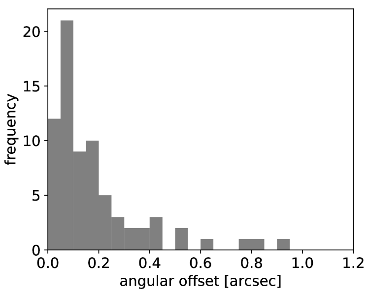
Figure 1: Angular offset in arcsec between the reported pointings of the SDSS aperture and COS/PSA. 85% of the objects show offsets smaller than the reported $1\sigma$ (68% of the distribution) accuracy of the absolute WCS of HST. The tail to high offsets is confirmed to correspond to WCS uncertainties. See text for details.

This study requires a quantitative comparison to be made between the UV and optical spectra, which we note have been obtained in slightly different apertures. The COS primary science aperture (PSA) has a diameter of 2$\aas@@fstack{\prime\prime}$5, and becomes vignetted at radii greater than $\approx$ 0$\aas@@fstack{\prime\prime}$6. Comparably to this, our SDSS spectra are observed in with 3$\aas@@fstack{\prime\prime}$0 fibers for 10% of the sample (with the SDSS spectrograph) and 2$\aas@@fstack{\prime\prime}$0 fibers for the remainder (9 galaxies, using the BOSS fibers). Concerning the positional alignment, we calculate the distribution of angular offsets, which we show in Figure 1. In the interpretation of this we first note that both telescopes performed acquisition centered upon the brightest local source, and we have verified in the COS acquisition images that the target was always acquired and centered to within a precision better than 3 NUV pixels (0$\aas@@fstack{\prime\prime}$066). However we also note that the absolute astrometric solution of the HST focal plane is $\approx$ 0$\aas@@fstack{\prime\prime}$25, while typical ground-based astrometric solutions are usually good to an rms of $\approx$ 0$\aas@@fstack{\prime\prime}$3. Assuming wavelength invariance of the morphologies, we would expect differences of $\approx$ 0$\aas@@fstack{\prime\prime}$4 (1–$\sigma$) between reported COS and SDSS coordinates in case of perfect aperture matching, purely as a result of differing WCS solutions. In light of this, it is surprising that the average offset in Figure 1 is as small as it is. We anyway inspect the SDSS fibre-positions of the nine objects with reported offsets more than  0$\aas@@fstack{\prime\prime}$4, and in fact find no evidence that the aperture centers actually differ by the reported amounts – we have verified that the tail of this histogram is due to the reported HST world coordinate system.

We next examine photometric issues: the size of the apertures with respect to the seeing. The median seeing of the SDSS survey is 1$\aas@@fstack{\prime\prime}$43, from which we calculate at 4.7% flux loss when feeding a fibre of 3" if the objects are point-sources. While there is no need for the underlying galaxy to be point-like, the overwhelming majority of COS acquisition images show the morphology of UV light would not be resolved from the ground. The sources are so compact in the UV continuum that the spectrophotometric effects of the COS vignetting function are negligible, and our spectral modeling (described in Section 3.1) will not be affected. However the same may not be true for Ly$\alpha$, which may be spatially extended with respect to the continuum. We examine the COS vignetting function, and calculate that for a flat surface of Ly$\alpha$ emission, 70% of the light would be recovered, although we estimate this loss to be somewhat conservative because the Ly$\alpha$ should also be centrally concentrated. We conclude that this effect remains as a systematic source of uncertainty that would enter at the $\approx 20$ % level on average, but without explicit information on the Ly$\alpha$ light profile we are unable to quantify the effect further.

Finally we remark that while we study a large number of properties in this paper, only one – the Ly$\alpha$ escape fraction, $f_{\mathrm{esc}}^{\mathrm{Ly}\alpha}$ – is actually sensitive to the relative flux calibration of COS and SDSS. Other UV properties are either equivalent widths or kinematic properties, while all the optical properties are line ratios, and aperture effects will mostly cancel out when the ratios are taken.

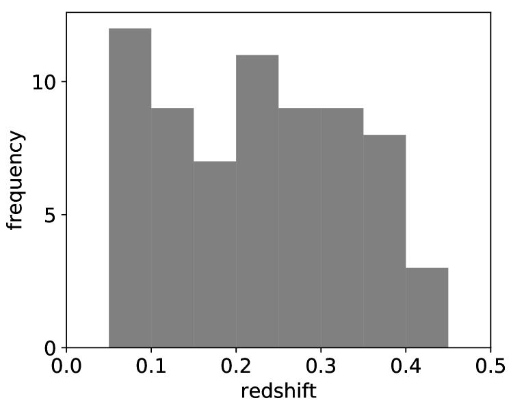
Figure 2: Redshift distribution of the galaxies. The upper limit is imposed by the necessity of having Ly$\alpha$ fall in the G160M grating of COS ($z<0.44$), while the lower limit is imposed by us to ensure that the bulk of the galaxy is encompassed within the aperture.

3 Data Processing and Measurements

3.1 Stellar Continuum Modeling

3.1.1 Motivation

The first step in our data processing is to model the continuum of the galaxies and estimate the properties of the stellar population. This serves a number of purposes. Firstly the modeling estimates and corrects for the stellar absorption features in the optical spectra, especially the Balmer and Paschen series of H i, and optical He i lines. This naturally improves the measurements of these emission lines. Secondly, we derive a model of the ultraviolet continuum that is free from interstellar absorption and emission lines. This is especially important near the high-ionization UV lines such as N v ($\lambda\approx 1240$ Å), Si iv ($\lambda\approx 1400$ Å), and C iv ($\lambda\approx 1550$ Å), which may mix contributions of stellar wind features, interstellar absorption, and nebular emission. The narrow interstellar and nebular lines are masked during the fitting process, leaving the much broader (several thousand km s^-1) P Cygni features to be modeled without contamination.

Thirdly, these models directly estimate the recent star formation history and stellar metal abundances, both of which are key quantities to investigate. Moreover, the direct estimate of the starburst age provides us with an independent route to obtain the instantaneous ionizing photon production rates (e.g. $Q_{0}$ for H i) and the mechanical energy returned to the interstellar medium by both winds from massive stars and supernova explosions. Inferences from these quantities were the subject of Hayes (2023) and the software formed the basis for calculations in Sirressi et al. (2022). Finally we also obtain a measurement of the internal dust reddening experienced by the stellar continuum, in addition to the nebular reddening from H i Balmer emission. As well as estimating physical properties, we also use these accurate models of the UV and optical continuum to normalize the observed spectra to measure interstellar absorption lines (see Section 3.4), and subtract the stellar continuum to measure nebular emission line fluxes (see Section 3.2). The process therefore corrects for P Cygni stellar features in the UV and stellar Balmer absorption in the optical.

3.1.2 Stellar Fitting Method

Our software fits multiple generations of stellar population, their ages, metallicity ($Z$), and dust obscuration. We adopt the high resolution libraries of Starburst99 (Leitherer et al., 1999; Vázquez & Leitherer, 2005; Leitherer et al., 2014), computed using the evolutionary tracks of the Geneva group for high mass-loss rates. We adopt a Salpeter initial mass function (IMF) between mass limits of 0.1 and 100 M_⊙, and permit metallicities across the full range of model libraries: $Z\in\{0.001,0.004,0.008,0.020,0.040\}$. We remind the reader that the evolutionary tracks from the Geneva group are computed using the outdated solar abundance patterns, and there may be a factor of $\approx 0.2$ dex offset (Asplund et al., 2009) when scaling between metallicity expressed as mass fraction ($Z$) and the oxygen abundance. The optical spectra include nebular continuum by default, under the assumption that 100% of the ionizing photons are reprocessed into nebular light that is emitted cospatially with the starlight.

We first mask the regions of the observed spectrum that are contaminated by known strong nebular emission and interstellar absorption lines. Milky Way absorption lines are also masked in the UV spectra. Stellar modeling then proceeds by first building a 3-dimensional data structure holding the luminosity density ($L_{\lambda}$) as a function of stellar age, metallicity, and wavelength ($\lambda$). We fit a 3-dimensional cubic spline field to this cube to build a interpolation function that produces $L_{\lambda}$ as a function of these three main quantities (age, $Z$, $\lambda$). This numerically differentiable function can then be used in standard minimizer algorithms, for which we adopt lmfit in Python.

The next step is to redshift the stellar models into the observed frame of the galaxies, and scale the luminosity density by a factor of $4\pi d_{\mathrm{L}}^{2}(1+z)$ (where $d_{\mathrm{L}}$ is the luminosity distance) to obtain spectra in flux densities ($f_{\lambda}$). We model the UV and optical spectra simultaneously so as to take advantage of the long spectral baseline afforded by the combined data ($\sim 1200-7000$ Å). This is firstly designed to estimate (or place limits upon) the presence of a more evolved underlying stellar population with higher mass-to-light ratio, and secondly to improve estimates of the stellar obscuration with the longer lever-arm in wavelength than using the UV data alone.

It is important to account for the fact that the COS and SDSS spectrographs have different spectral resolutions (by a factor of $\sim 5$ depending upon the light distribution of the source). Our fitting algorithm includes the intrinsic velocity dispersion of the stellar population as a free parameter, which is implemented by a two-step convolution. Within the function that generates the spectrum, we first convolve with a single Gaussian (to account for intrinsic stellar velocity dispersion), and then by the resolutions of the independent spectrographs: the UV models are convolved to $R\approx$ 12,000 (approximately that of HST/COS), while the optical spectra are convolved to $R\approx$ 2,000, which holds for the SDSS spectrograph at the central wavelength of interest ($\lambda\approx 5000$ Å).

Star formation is an inherently clustered process, with starbursts typically forming stars in a number of discrete star clusters. This is especially obvious at ultraviolet wavelengths (e.g. Meurer et al., 1995), and we may expect multiple populations of stars to exist within the COS aperture. The youngest stars dominate the light output, but more evolved massive stars (down to B-type, with ages to 40 Myr) may be more important in determining the mechanical energy release if supernova contribute significantly. Thus the more evolved population cannot be ignored (see Sirressi et al., 2022). When fitting just one population of stars, the stellar ages are almost always found to be 3–4 Myr, and are drawn to this value by the strong P Cygni lines (e.g. N v, C iv) that form in the winds of the most massive stars. However these wind lines represent only a tiny minority of the wavelength coverage: a lot of information is also present from narrower photospheric lines that are much weaker but far more numerous, as well as the overall shape of the continuum (see Chisholm et al., 2019; Senchyna et al., 2022). As we expect more protracted episodes of star formation (free-fall timescales are $\gtrsim 10$ Myr), we fit the additive combination of one, two, and three stellar populations to the data, selecting the final model with the lowest $\chi^{2}$ per degree of freedom as the final model. In order to better estimate the star formation history over timescales relevant for mechanical energy return and the development of galaxy winds, we allow the ages to range freely over the limits of $10^{6}$ to $10^{10}$ yr.

We redden the spectra using the dust attenuation law derived for starburst galaxies by Calzetti et al. (2000); we have experimented with other parameterizations, such as Charlot & Fall (2000) and clumpy dust distributions (Natta & Panagia, 1984, revisited for Ly$\alpha$ emitting galaxies by Scarlata et al. 2009) without a noticeable increase in the quality of our fits. We apply the same dust attenuation to each stellar population. We acknowledge this as a limitation of method, but large degeneracies are introduced when fitting multiple extinctions that effectively decouple the optical and UV spectra. This leads to very different extinctions at fixed age, and very different stellar metallicities that are also hard to motivate. We show an example of the ultraviolet spectral modeling in Figure 3.

3.1.3 Summary of Estimated Properties

In total we measure and record:

Normalization of each stellar population. This is recovered directly from the modeling. Since we fit simple stellar populations from Starburst99, this corresponds directly to a stellar mass, which we have for the total population (all ages) and ‘starburst event’ (defined as ages below 20 Myr).

Stellar Age. This is recovered directly from the modeling. With the normalizations computed above and relative contributions of light at different wavelengths, we can then describe the total population with mass or light-weighted ages.

Stellar Metallicity. As with ages, this is a basic fit parameter and can be assembled into mass- and light-weighted descriptors of the population.

Total stellar attenuation. This is a basic result of the fitting that is recovered directly assuming the Calzetti et al. (2000) prescription.

Ionizing photon production rates. Starburst99 tabulates the production rates of H-, He-, and H⁺-ionizing photons as a function of age and metallicity. We compute these quantities, which we refer to as $Q_{0}$, $Q_{1}$, and $Q_{2}$, respectively, using the quantities estimated above; as with all properties we have an estimate for each population and the sum over all stars.

Mechanical energy return. Similarly, Starburst99 also tabulates the instantaneous mechanical luminosity, which we refer to as $L_{\mathrm{mech}}$. We treat $L_{\mathrm{mech}}$ in the same way as ionizing photon rates above, and sum to obtain the current value. However mechanical luminosity is the time derivative of the energy, and by integrating $L_{\mathrm{mech}}$ along the evolution Starburst99 tables, we can compute the total energy deposited by each stellar population at its estimated age. We refer to this as the integrated mechanical energy, $E_{\mathrm{mech}}$.

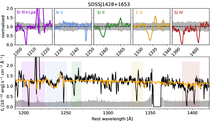
Figure 3: Spectral modeling of the stellar continuum, using well-exposed object SDSS J1428. The lower panel shows the observed UV spectrum in black, shifted into the restframe. The model fit is in orange, and the uncertainty level is indicated by the grey shaded region. Large deviations from the fit are mostly caused by ISM absorption features, fluorescent emission lines, and Ly$\alpha$. Upper panels show zooms around some relevant features, each of which is labeled, and colors correspond to the shaded regions in the lower panel.

3.2 Optical Emission Lines

3.2.1 Measurements

After subtraction of the stellar continuum, we measure many relevant nebular emission lines. These range in wavelength between the [O ii]$\lambda\lambda 3726,3729$ Å doublet in the blue, and the Pa 8 line at 9229 Å, but what lines are actually measured for a given galaxy depends on redshift. There are 42 lines in total, the highest ionization potential of which is that of He ii $\lambda 4686$ Å with IP=54 eV, although also includes other lines of Ar³⁺ and Ne²⁺ that also probe particularly highly ionized gas phases. The stellar modeling described in Section 3.1.2 automatically corrects for underlying absorption in the Balmer lines.

We perform a simultaneous kinematic fit to all the emission lines. We fit one single recession velocity (redshift) and Gaussian FWHM to represent the velocity dispersion of the gas. We account for the wavelength-dependence of the spectral resolution by interpolating the estimated resolving powers (provided in the instrument manuals) to the observed wavelength of each line, and convolve each model line with the instrumental resolution. For each line, the only free parameter is the normalization, which then gives the flux. Fitting the sum of these lines to the data we automatically deblend nearby lines (e.g. H$\alpha$ and [N ii]) and get a better estimate of the total [O ii] flux by partially deblending the doublet. We estimate errors using a Monte Carlo simulation, where we use the error spectrum to weight a regeneration of each pixel in the spectrum using randomized Gaussian deviates.

Some of the strongest lines are clipped by the SDSS data reduction pipeline, where they are mis-identified as cosmic rays. These are relatively easy to identify as either absent entries in the error vector, or unphysical ratios for the strongest lines. We fix clipped 5007 Å lines using 2.98 times the flux of the 4959 Å line, and clipped H$\alpha$ lines in a handful of cases are repaired by estimating the nebular reddening from the H$\gamma$/H$\beta$ ratio and scaling dust-corrected H$\beta$ flux and re-applying the reddening suitable for 6563 Å.

3.2.2 Estimated Nebular Conditions

We examine a large number of commonly used line ratios, and are specifically interested in:

Specific star formation rate/stellar evolutionary phase. Formally we have these quantities estimated from the stellar modeling above, but we also compute equivalent values from the emission lines. We estimate the SFR from dust-correct H$\alpha$ (see below) using the calibration of Kennicutt & Evans (2012). We record the EW of all emission lines: the H$\alpha$ EW strongly correlates with the sSFR and H$\beta$ EW strongly with the evolutionary stage. We also examine the EW of the strong [O iii]5007 line, as it is so complicit in the selection of galaxies at both low- and high-redshifts.

Abundance of dust and metals. We use the H$\alpha$/H$\beta$ ratio that traces dust reddening, and adopt the extinction curve of Cardelli et al. (1989). We also record ratios that predominately trace ionic abundance: [N ii]6484/H$\alpha$ ($N_{2}$), [S ii]6717,31/H$\alpha$ ($S_{2}$), and combinations of [O iii]/H$\beta$ ($R_{3}$) and ([O iii]+[O iii])/H$\beta$ ($R_{23}$).

Ionization state. We include basic ratios of lines that have very different ionization potentials, and may encode information on the ionization levels of the gas. We use recombination lines (RLs) such as He i/H$\beta$, and He ii/H$\beta$, and commonly used ratios of collisionally excited lines (CEL), such as [O iii]/[O i] ($=$O₃₁), [O iii]/[O ii] ($=$O₃₂), [Ne iii]/[O ii] (Ne3O2), and [Ar iv]/[Ar iii] (hereafter Ar₄₃).

Optical depth tracers. We record the ‘S ii deficit’ (Wang et al., 2019; Wang et al., 2021), which is defined as the logarithmic distance of a galaxy in [S ii]/H$\alpha$ from the sequence of galaxies in the plane of [O iii]/H$\beta$ vs. [S ii]/H$\alpha$. As such, it approximately encodes the lack of [S ii] emission at fixed metallicity and ionization state, which could imply low column densities as the partially neutral medium is truncated. We also add the ratios of He i lines 3888/6678 and 7065/6678, which have both been shown by Izotov et al. (2017) to be subject to transfer effects.

Thermodynamic variables. We calculate electron density ($n_{\mathrm{e}}$) from [S ii] 6717/31 ratio and electron temperature ($T_{\mathrm{e}}$) from [O iii]4363/5007 ratio using the iterative method in PyNeb (Luridiana et al., 2015). We calculate pressure ($P_{\mathrm{e}}$) from the product of the two.

3.3 Lyman alpha Measurements – the Dependent Variables

We make most of our measurements concerning the Ly$\alpha$ emission (fluxes, equivalent widths, and kinematic properties) using Lyman alpha Spectral Database (LASD, Runnholm et al., 2021) and refer the reader to that paper for a detailed description. In summary we rely upon the following quantities:

Ly$\alpha$ luminosity. This is computed by numerical integration of the continuum-subtracted spectrum over a 2500 km s^-1 window centered around the systemic velocity. This quantity, and all that follow from it, also includes any interstellar Ly$\alpha$ absorption – I.e. Ly$\alpha$ absorbed out of the stellar continuum (most frequent at $v<0$) subtracts from the net Ly$\alpha$ flux.

Ly$\alpha$ equivalent width. This follows from luminosity computed above. Continuum placement is handled using clipping algorithms inside of the LASD, and interpolated to 1216 Å. In this paper we adopt the ‘nebular definition’ of EW, that emission is positive.

Ly$\alpha$ escape fraction, $f_{\mathrm{esc}}^{\mathrm{Ly}\alpha}$. This is computed using dust-corrected Balmer line emission. For this we use the prescription defined in Hayes et al. (2005) as $f_{\mathrm{esc}}^{\mathrm{Ly}\alpha}=L_{\mathrm{obs}}^{\mathrm{Ly}\alpha}/(8.7\times L_{\mathrm{int}}^{\mathrm{H}\alpha})$, where $L_{\mathrm{obs}}^{\mathrm{Ly}\alpha}$ is the observed Ly$\alpha$ luminosity, $L_{\mathrm{int}}^{\mathrm{H}\alpha})$ is the intrinsic (dust corrected; see Section 3.2) H$\alpha$ luminosity. The factor 8.7 stems from the intrinsic Ly$\alpha$/H$\alpha$ ratio (see arguments in Hayes, 2015).

The first moment. This characterizes the velocity shift relative to line centre and is calculated over the same wavelength range as above.

The second moment. This characterizes the velocity width of the line and is calculated over the same wavelength range as above.

The third moment. This quantity, commonly known as the skewness, characterizes the asymmetry of the emission line. It is is calculated over the same wavelength range as above.

As well as integrated over the entire spectral region (full width of 2500 km s^-1), we also calculate all these quantities for the negative-only and positive-only velocities, which we refer to as blue and red components. We acknowledge that it may not be clear how to interpret some of these quantities when divided into the blue and red parts, as frequency redistribution can shift wave packets across line centre. We therefore emphasize that these flux-related quantities should be thought of as the contribution of the blue/red-shifted emission to the total output Ly$\alpha$.

3.4 UV Continuum Measurements – ‘Explanatory’ Variables

We use ultraviolet absorption lines to explain the phenomena we see when contrasting nebular measurements with the Ly$\alpha$, and focus on three species: Si ii$\lambda 1260$ Å, C ii$\lambda 1334$Å, and Si iv$\lambda 1403$ Å. The former two ions have relatively low ionization potentials: Si⁺ requires 8.2 eV to be produced, and requires 16.3 eV to photoionize to Si²⁺; the corresponding range for C⁺ is 11.3–24.4 eV. The Si⁺ and C⁺ zones therefore overlap with the neutral zone of hydrogen (0–13.6 eV). Si iv, on the other hand, requires at least 33.5 eV to be produced and probes gas ionized by higher energy radiation, potentially with a significant contribution from collisional processes. The stellar modeling described in Section 3.1.2 automatically corrects for contamination of narrow interstellar features by broad P Cygni wind lines.

Unfortunately, the individual UV spectra do not have sufficient signal-to-noise ratio in the continuum to well measure these absorption lines target-by-target. We therefore rely upon a stacking analysis, similar to that performed for Ly$\alpha$ (Section 6.1.1). Because of the required stacking we cannot treat these as independent variables upon which to base a differential comparison, but use them to further explain the trends seen in Ly$\alpha$; we therefore refer to these measurements as explanatory variables, and investigate them in a post-hoc fashion.

The absorption line studies are concerned with the relative strength compared to the continuum itself, so we perform continuum normalization prior to analysis (in contrast to the continuum subtraction performed for the Ly$\alpha$ measurements). This is done by dividing out the best fitting Starburst99 model described in Section 3.1, which leaves a normalized spectrum that is free from stellar features and contains only interstellar lines (see the insets of Figure 3). In the normalized spectra we measure:

Equivalent width of absorption lines. The flux is computed by direct numerical integration, and divided by the continuum level (in normalized spectra this is anyway set to 1). We conduct the integral over a velocity range of $-800$ to $+200$ km s^-1. This asymmetric window may appear as though it would bias our results, however (1.) no absorption is seen in our spectra at velocities higher than 200 km s^-1, as the overwhelming majority of the absorption is blue-shifted. Moreover (2.) there is a fluorescent emission line from C ii 280 km s^-1 red-ward of the resonance absorption line, that would contaminate our measurement. Note that for our definition, the absorption lines have negative EW.

Velocity offset of absorption lines. We take the first moment of the absorption line, computed over the same window as described above. This provides an estimate of the characteristic velocity at which the bulk of the foreground gas is outflowing.

Absorbed fraction at zero velocity. In normalized spectra, this is just the flux density measured at $\Delta v=0$, and encodes the amount of foreground gas that is static (recall that the systemic redshift is derived from optical line emission). We take the direct average of the four resolution elements closest to $\Delta v=0$ (two at positive and two at negative velocities).

Equivalent width of fluorescent emission lines. For the Si ii and C ii lines we also compute the EW of their fluorescent counterparts, in exactly the same way as for the absorption lines above. More details can be found in Section 7.3.

4 Results I – Properties of the Sample from Stellar and Nebular Spectroscopy

4.1 Ionization Conditions and Nebular Excitation

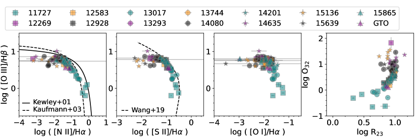
Figure 4: BPT and excitation diagrams. The three common diagnostic diagrams of Baldwin et al. (1981) are shown, along with the excitation diagram of Nakajima & Ouchi (2014) to the far right. The BPT diagrams all show the log of the [O iii]/H$\beta$ ratio on the ordinate axis. Abscissae show the [N ii]/H$\alpha$, [S ii]/H$\alpha$, and [O i]/H$\alpha$ ratios. Demarcation lines of Kewley et al. (2001) and Kauffmann et al. (2003) are shown that segregate starburst galaxies from AGN in the upper left figure, while the line defining the [S ii]-deficit (Wang et al., 2019) is shown in the second diagram. The far right figure shows the logarithm of the [O iii]5007/[O ii] ratio vs. the ([O ii]+[O iii]4959,5007)/H$\beta$ ratio, specifically used to show the most highly ionized ISM conditions towards the upper right. Program identifiers for the individual COS programs are indicated using various colors and symbols (labelled in the legend).

We begin by characterizing the sample, using the stellar and nebular properties derived in Section 3. We show the commonly-used sequence of diagnostic diagrams (Baldwin et al., 1981), hereafter ‘BPT-diagrams’, in Figure 4. These figures encode the ionization conditions, excitation, and metallicity along various loci. Upper left shows the [O iii]/H$\beta$ vs [N ii]/H$\alpha$ plane that is typically used to identify star-forming galaxies from AGN, demarcated by theoretically and observationally determined functions (Kewley et al., 2001; Kauffmann et al., 2003, respectively). Galaxies are spread along the star-forming sequence. A handful of galaxies do cross into the AGN-dominated regions, but none exceed the higher curve by more than $1\sigma$, and there is little indication of AGN contamination in the sample. Program identifiers from the HST observational campaigns are coded by various symbols and colors: 11727 and 13017 spread to more metallic and low excitation end of the diagram, where cooling is more efficient. In contrast, programs targeting low-mass and metallicity, highly excited starbursts fall at the upper left end of the diagram.

The upper right plot shows a similar pattern, with galaxies falling along a narrow sequence. The dashed line was defined in Wang et al. (2019), and represents a fit to all the star-forming galaxies in the SDSS spectroscopic samples. All galaxies fall close to, or somewhat to the left (‘[S ii]-deficient’) side of the line. This deficit is most clearly visible in GO 15136 and 15639, which were both selected to be LyC- and Ly$\alpha$-emitting candidates with the most highly ionized interstellar media; they were not, however, selected by $\Delta$[S ii].

The lower right panel shows where the galaxies fall in the plane of [O iii]/[O ii] (O${}_{32})$ vs ([O ii]+[O iii])/H$\beta$ (R₂₃) ratios. Similar to the BPT diagrams, this ‘excitation diagram’ encodes the level of excitation on both axes, while the ordinate includes an additional factor of nebular metallicity. It therefore appears as a rotated version of the BPT locus. The diagnostic diagram has been used extensively as an indicator for potential LyC leakage as it identifies highly ionized interstellar media (e.g. Nakajima & Ouchi, 2014).

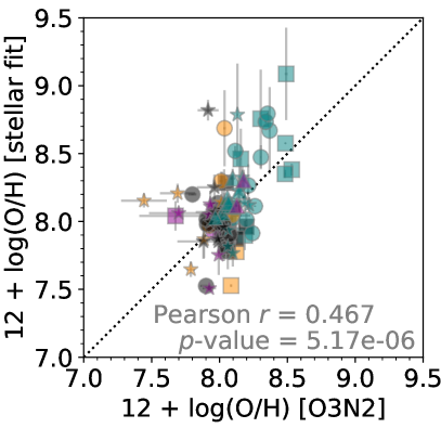
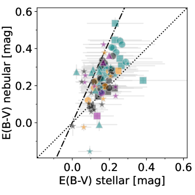
Figure 5: Left shows a comparison of stellar and nebular metallicity estimates. This example shows O3N2 strong-line calibration vs the estimates made by fitting the stellar continuum. Note that stellar metallicities were estimated using models calculated with the outdated solar oxygen abundance of $12+\log(\mathrm{O/H})=8.9$. Right shows a comparison of stellar and nebular dust attenuation estimates. This example shows $E_{B-V}$ derived from the H$\alpha$/H$\beta$ ratio against that corresponding value derived by modeling the stellar spectra. Dotted lines show equivalence in both cases, while the dot-dashed line in the right panel shows nebular nebular extinction at 2.2 times the stellar value (see text for details). The color and shape coding of the markers are the same as in Figure 4.

4.2 Heavy Element Abundances and Dust Obscuration

In the left panel of Figure 5 we show how the metallicities compare when derived using stellar and nebular methods. For the nebular gas we adopt the strong-line method of the O3N2 index ([O iii]5007/H$\beta$ $\times$ H$\alpha$/[N ii]6584), using the calibration of Marino et al. (2013). While we have made estimates using temperature sensitive methods, the faintness of the [O iii]4363 feature in many of our galaxies means this method is of little use for comparing galaxies at very different distances. Overall there is reasonable agreement around 12+log(O/H) $\approx 8.0$, but the scatter is large at all abundances. Pearson’s $r$ coefficient, which measures the degree of linearity between the two measurements recovers a $p$-value of $5.2\times 10^{-6}$, but it is noteworthy that at higher metallicities the stellar methods tend to estimate higher metallicities. Moreover by eye it appears that the relation between the two measurements is steeper than the 1–1 slope.

It has been noted at high-redshifts that metallicities derived from stellar continua tend to be lower than those derived in the gas. Steidel et al. (2016) show that stellar metallicities fall below those of the nebular phase by a factor of 3–5 for $z=2-3$ Lyman Break Galaxies (LBG). They attribute this phenomenon to enhancement of alpha-based products of nucleosynthesis in young star forming events, suggesting that the recent explosion of many core-collapse supernovae have enriched the ISM with oxygen (which dominates nebular measurements in the optical). In contrast the lack of thermonuclear supernovae results in a relative absence of iron, which is the dominant source of opacity in stellar atmospheres and the main source of metallicity information in ultraviolet stellar fitting. In similar lower redshift studies that use similar techniques, Chisholm et al. (2019) do not find this lack in stellar metals: they instead report very tight, linear agreement between stellar and nebular metallicities, suggesting that the enrichment processes occur on longer timescales.

The right panel of Figure 5 shows how the stellar and nebular estimates of the dust attenuation compare. There is generally a strong trend between the two estimators, although they clearly do not align along the one-to-one relation (dotted line), and nebular attenuation is typically higher than that of the stars. In fact, the locus of points is closely aligned with a factor of 2.2 scaling between the nebular and stellar values. This is consistent with results from local starburst galaxies (Calzetti et al., 2000; Kreckel et al., 2013, see also discussion in Reddy et al. 2015). We note, however, that there is a slight offset between the locus of points and the 2.2-scaling line, of about $\Delta E_{\mathrm{B-V}}\approx+0.05$ mag in the nebular value. Both the general slope and offset are confirmed when replacing the H$\alpha$/H$\beta$ ratio with that of H$\gamma$/H$\beta$. This offset remains unexplained, but we speculate it could be due to the differing relative geometries of stars and gas that may be implicit in our sample compared to those of more local starbursts where these comparisons have more-often been performed.

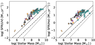
Figure 6: The relationship between stellar mass and star-formation rate. Stellar mass is always derived from spectral modeling. Left: the UV-based SFR, corrected for stellar reddening derived from stellar population fitting. Right: the H$\alpha$-based SFR, corrected for nebular reddening using the H$\alpha$/H$\beta$  ratio (or H$\gamma$/H$\beta$ on occasion). Linear fits to the same relation at redshifts 1,4, and 5 are shown by increasing lines, derived by Santini et al. (2017). The color and shape coding of the markers is the same as in Figure 4.

4.3 Mass and SFR Relations

Figure 6 shows the relation between star formation rate and the stellar mass, sometimes referred to as the star-forming main sequence. Stellar masses are derived routinely from the continuum measured in the COS and SDSS spectroscopic apertures (Section 3.1.2), and must On the left we show the SFR derived from the UV continuum flux, corrected for dust attenuation on the continuum, and using the calibration of (Kennicutt & Evans, 2012). The right figure shows the SFR estimated using the H$\alpha$ luminosity, corrected for dust using the H$\alpha$/H$\beta$ (or on occasion the H$\gamma$/H$\beta$) ratio. Overlaid are relations derived at redshifts 1, 4, and 5 by Santini et al. (2017), which increase in their normalization with redshift, but otherwise follow a very similar slope.

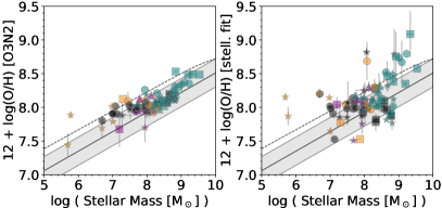
Figure 7: The mass-metallicity relation. Left shows the metallicity derived from the O3N2 index, and right shows the metallicity derived from the stellar fitting (see also Figure 5). Note that stellar metallicities were estimated using models calculated with the outdated solar oxygen abundance of $12+\log(\mathrm{O/H})=8.9$. The solid line and shaded region shows the low-$z$ relationship derived from the Local Volume Legacy Survey (Berg et al., 2012), while the single dashed line is the relationship of Curti et al. (2020). The color and shape coding of the markers are the same as in Figure 4.

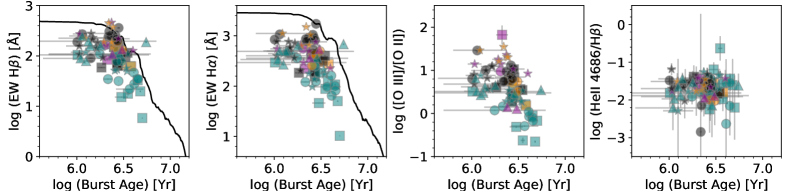
Figure 8: The evolution of some characteristic optical observables with derived age of the starburst component (younger). Far left shows the equivalent width of H$\beta$ and centre left the EW of H$\alpha$. The EWs have been corrected for the differing levels of dust attenuation experienced by the stars and gas, which are estimated independently by stellar modeling and the Balmer decrement. The tracks correspond to instantaneous burst Starburst99 models for $Z=0.008$ and a Salpeter initial mass function. Center right shows the O₃₂ ratio and far right the ratio of He ii4686/H$\beta$. The color and shape coding of the markers are the same as in Figure 4.

Our sample is offset from the SFR-stellar mass relations in the direction of higher SFR at fixed mass. Here we caution that our methods and selection are both very different from those applied in other studies. Firstly in selection, some of these objects are identified as being among the most extreme starburst events present in the local universe. They have the highest equivalent widths in the optical emission lines (H$\alpha$ and [O iii]), which would naturally shift the locus of points to higher values, especially compared to the lower redshift sequences. Secondly the stellar masses are measured in small apertures corresponding to 1$\aas@@fstack{\prime\prime}$25 in radius. Our modeling is designed to recover the recent star formation history by fitting multiple populations of stars; this should add more leverage to capture underlying stellar populations, but may still remain biased towards the youngest population with the lowest mass-to-light ratio. This should accurately reproduce the burst mass, but is likely to leave the total stellar mass underestimated, shifting galaxies towards the left on this Figure.

Figure 7 shows the mass metallicity relation (MZR), including metallicities derived by both strong line calibrations (left) and stellar continuum modeling (right). The overlaid relations are derived from SDSS galaxies (Curti et al., 2020, dashed black line) and for dwarf galaxies in the Local Volume Legacy Survey (Berg et al., 2012, black line). The agreement with the MZR for local galaxies is surprisingly good, given the lack of agreement with the SDSS-derived SFR-$M_{\mathrm{stell}}$ relation (Figure 6). Together these figures suggest that the disagreement in Figure 6 is actually not because the mass has been underestimated because of aperture effects, but because the SFR is elevated compared to typical local galaxies of equivalent stellar mass.

Based upon the SFR main sequence (Figure 6) we could expect our sample to lie above the $z=0$ MZR, since they are currently producing more metals than the average galaxy at fixed mass. This is true, but only marginally so: points appear to occupy roughly the upper half of the grey band describing local dwarfs. At higher redshifts, however, the MZR evolves towards lower metallicity at fixed mass (Erb et al., 2006; Maiolino et al., 2008). Thus, while a agreeing reasonably with the local MZR, our sample diverges from the mass-metallicity relation seen at higher redshifts.

Figure 8 shows how some nebular quantities evolve with starburst age. For age, we adopt that of the starburst (youngest) population that provides the majority of the hydrogen-ionizing photons. We first show the the equivalent widths of the Balmer lines, H$\beta$ and H$\alpha$, which should drop rapidly when the most massive and ionizing stars explode. In this figure only we take the unconventional step of correcting the EWs for dust, using the independently-derived stellar attenuation (from modeling) and nebular reddening (calculated from the H$\alpha$/H$\beta$ ratio). It is often noted that inferred absorption due to dust is higher when measured from the nebular gas when compared with stellar light. This is believed to be the result of geometrical effects (e.g. Calzetti et al., 2000), and is also verified in this sample (see Section 4.2).

We overplot Starburst99 evolutionary tracks for the same quantities (Leitherer et al., 1999). It is clear that the theoretical track always over-predicts the EW, in an effect that is stronger for H$\alpha$ than for H$\beta$. We believe this is mostly because the redder wavelengths include larger contributions from more evolved stars: the multi-component modeling described in Section 3.1.2 does account for a more evolved population, and we confirm that strong absorption is seen (typically H$\epsilon$ to about H12) in the high-order Balmer lines in these cases. This is consistent with dilution of the EWs typical of single-population starbursts. Moreover, the escape of ionizing photons can also reduce the EW of recombination lines while leaving all colors basically unaffected (e.g. Bergvall et al., 2013). While this scenario is possible, we do not expect escape fractions to typically be high enough to cause significant reductions to the observed EWs. It is encouraging to see such agreement for the H$\beta$ line where the contamination is lower than for H$\alpha$, which would be expected in the case of contamination from cooler stars. Overall, we interpret these findings as support for the spectral modeling, reinforcing the belief that it has produced acceptable ages for the hard-to-model starburst component, and reasonable production rates for hydrogen-ionizing photons.

The centre right plot shows the time-evolution of the O₃₂ ratio, which also decreases substantially with time. Like Balmer line fluxes, this ratio peaks at very early times when stars produce more $h\nu\geq 34.4$ eV photons that can doubly ionize oxygen. In this case it may be tempting to attribute the evolutionary effect directly to an excess of photons at $h\nu\geq 34.4$ eV compared to 13.6 eV. The far right plot, however, shows this interpretation unlikely to be correct as the same phenomenon is not noticed when comparing recombination lines of He ii (54.4 eV) with hydrogen. This result mirrors that of Marques-Chaves et al. (2022), who find that the He ii/H$\beta$ ratio does not correlate with either the ionizing escape fraction, while the O₃₂ ratio in the same sample does (Flury et al., 2022). We expect, therefore, that the evolution of O₃₂ seen here is instead related to a truncated O⁺ zone, as the O²⁺ region is elevated due to large scale photoionization in younger galaxies.

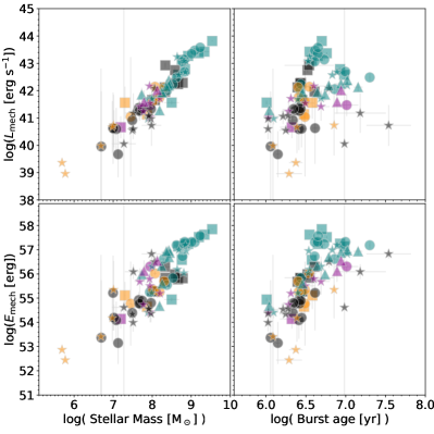
Figure 9: The mechanical energy return from stellar feedback. The upper row shows the instantaneous rate of energy injection (mechanical luminosity) from stellar winds and supernovae, projected against the mass formed in the starburst (left) and age of that population (right). The lower row shows the integral of the mechanical luminosity over time since the onset of the burst (the total mechanical energy injected). The color and shape coding of the markers are the same as in Figure 4.

4.4 Mechanical Luminosity and Kinetic Energy Return

With reasonable estimates of the mass and evolutionary point of the starburst episode, we estimate the rate of mechanical energy injection into the ISM as a result of stellar feedback processes (the mechanical luminosity, $L_{\mathrm{mech}}$). The total amount of mechanical energy returned since the onset of the starburst ($E_{\mathrm{mech}}$; see Section 3.1.3) then follows by integrating along the star formation history. We show the relations between {$L_{\mathrm{mech}}$, $E_{\mathrm{mech}}$} and {mass, age} in Figure 9. We recover a large range in $L_{\mathrm{mech}}$ between $10^{39}$ and $10^{44}$ erg s^-1, and as shown in the upper left panel, the bulk of this is explained almost linearly by the large range of burst masses. The dispersion on this relation is quite small and comes from the time-dependent instantaneous mechanical luminosity injection, which varies with dominant mode (stellar winds or supernova) and position along the (current) stellar mass function (see, for example, Figure 111 of Leitherer et al., 1999). We plot $L_{\mathrm{mech}}$ as a function of burst age in the upper right panel, which also shows a broadly positive correlation, in this case because the supernova explosion rate increases with time until about 40 Myr. The very large dispersion results from the large dynamic range in burst masses already discussed.

The lower panels in Figure 9 show the total mechanical energy injected since the onset of star-formation, again plotted against mass formed and burst age. The range of $E_{\mathrm{mech}}$ runs from $10^{52}$ and $10^{58}$ erg, which for comparison corresponds to the energy returned by $\sim 10$ to $10^{7}$ supernovae. The relation between total $E_{\mathrm{mech}}$ and mass is somewhat more dispersed than the corresponding relation with $L_{\mathrm{mech}}$, spanning a range of $\approx 2.5$ dex at $M_{\mathrm{stell}}$ $=10^{8}$ M_⊙. This expected, since $E_{\mathrm{mech}}$ is the integral of $L_{\mathrm{mech}}$ from $t=0$ to now, and depends more sensitively upon the time since the burst ignited – see the corresponding points in the lower right panel, which show this variation of $E_{\mathrm{mech}}$ with stellar age.

4.5 Summary of Estimated Properties

This section demonstrates that our combined sample of almost 90 starburst galaxies spans a large and useful range of the multi-dimensional parameter manifold. Galaxies span a broad range of positions on the BPT diagrams from the very low metallicity and highly excited end, to more ‘normal’, metal rich end. They trace the star-forming sequence throughout, with only a handful of partial exceptions. The sample spans around three orders of magnitude in stellar mass, from $10^{6}$ M_⊙ to more than $10^{9}$ M_⊙; it is true that these are aperture-based values and will be somewhat lower than the total mass in stars, but the burst mass in which we are most interested is likely accurately recovered. The SFR spans a similar dynamic range from 0.1 M_⊙ yr^-1 to around 100 M_⊙ yr^-1.

Metal abundances span a range of 12+log(O/H) $=7.5-8.5$, and the correspondence between gas phase metallicity is close to the trend that would be expected for dwarf galaxies at low-redshift. There is reasonable agreement between the gas-phase and stellar metallicities; while this need not necessarily be the case, the correlation is encouraging from the perspective of stellar modeling. It suggests that our efforts to break the age-metallicity degeneracy are successful, and that there is meaningful information to be extracted from the star-formation histories/stellar ages. This is important because it later feeds into the estimates of ionizing photon production rates and mechanical energy return. The conclusion is further backed up by the correspondence between inferred starburst age and independent estimates based upon the equivalent width of optical recombination lines.

5 Results II – Lyman Alpha Output and Fundamental Variables

In this section we characterize the sample in terms of the bulk Ly$\alpha$ properties, where we focus on the observables of Ly$\alpha$ luminosity and EW. We show this in Figure 10 to address the question of where the strongest Ly$\alpha$ emitting galaxies may be found, and to facilitate more direct comparison with high-$z$ observations.

The upper left figure shows $L_{\mathrm{Ly}\alpha}$ vs. $M_{\mathrm{FUV}}$, where dotted lines show constant EW, and the lower panel shows this EW directly. Note that the dashed lines do not precisely agree with the EWs measured in individual galaxies; for example the two galaxies with EW $<1$ Å in the upper figure have log(EW/Å) $\approx 0.2$ in the lower plot. The reason for the difference is that $M_{\mathrm{FUV}}$ is measured in GALEX data to provide the total magnitude, and therefore samples the UV continuum at observed wavelength of 1527 Å, regardless of galaxy redshift. The EWs, on the other hand, are measured in the COS spectra to cancel out any aperture effects, and estimate the restframe continuum flux density at restframe 1216 Å directly. While neither of these numbers is incorrect, the inconsistency arises because of the different restframe wavelengths and apertures sampled by COS and GALEX.

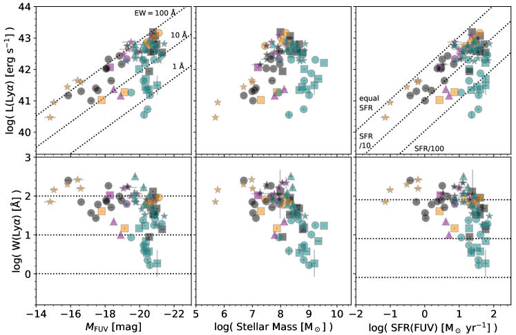
Figure 10: Variation of the total Ly$\alpha$ observables of luminosity (upper) and equivalent width (lower) with $M_{\mathrm{FUV}}$ (left), stellar mass (center), and SFR (right). Dashed lines on the left figures are of constant Ly$\alpha$ EW showing 1, 10, and 100 Å; comparable lines on the right plots show equivalent SFR in Ly$\alpha$ and FUV, and values for SFR(Ly$\alpha$) scaled down by factors of 10 and 100. Mass is derived from spectral modeling, UV magnitude is the observed quantity and has not been corrected for dust obscuration, while in the SFR calculation dust has been accounted for. See Section 5 for details. Color-coding shows the original proposal from which each FUV observation was drawn, and is consistent with Figure 4.

$L_{\mathrm{Ly}\alpha}$ does not scale directly with $M_{\mathrm{FUV}}$, but an upper envelope is clear, where a maximum value of $L_{\mathrm{Ly}\alpha}$ appears to be imposed at EW $\approx 100$ Å. Points typically scatter below this line, with EWs of several tens of Å, but scatter is larger towards higher luminosities. At $M_{\mathrm{FUV}}$ $\approx-21$ ($\sim$ $M^{\star}$ for $z=3$ LBGs, and 3 magnitudes brighter than $M^{\star}$ at $z=0$), Ly$\alpha$ luminosities reach their largest values of $\approx 10^{43}$ erg s^-1, which is also close to $L^{\star}$ for LAEs at $z\sim 3$ ($10^{42.7}$ erg s^-1; Herenz et al. 2019). However the lowest Ly$\alpha$ luminosities of $\approx 10^{40.3}$ erg s^-1 are also found at the same $M_{\mathrm{FUV}}$, corresponding to EWs as low as 1 Å. This dispersion, in which Ly$\alpha$ EWs range between $\sim 1$ and $\gtrsim 100$ Å is more visible in the lower left plot, and is driven largely by the inclusion of cyan points, corresponding to earlier COS programs (11727 and 13017) that targeted more massive LBG-like galaxies. We see less dispersion in $L_{\mathrm{Ly}\alpha}$ and EW towards the fainter end of the $M_{\mathrm{FUV}}$ distribution, where the sample is dominated by galaxies selected to have more highly ionized ISM (e.g. 15136 from Izotov et al. 2020, and 14080 from Jaskot et al. 2017). We do not claim that comparably low EW Ly$\alpha$-emitters do not exist among such faint galaxies: this is probably a result of sample selection where these objects, while faint, have been identified by having the highest production efficiencies of ionizing radiation among all the known samples. We confirm this directly in Sections 6 and 7.

A similar distribution of points is visible in the central two panels of Figure 10, which shows the variation of Ly$\alpha$ with respect to mass. The $L_{\mathrm{Ly}\alpha}$ vs. $M_{\mathrm{stell}}$ figure, however, shows a less clear upper envelope, and the upper-right corner of the EW distribution is no longer populated. Both these differences can be attributed to the cyan points (again 11727 and 13017), which exhibit higher stellar masses than other samples of comparable UV luminosity. This higher mass-to-light ratio is the result of a more evolved stellar populations in these sub-samples, as demonstrated in Figure 8 – it is likely that part of the reason these galaxies less luminous in Ly$\alpha$ and showing lower EWs is because less Ly$\alpha$ is produced intrinsically by the more evolved population.

The right panels of Figure 10 show the $L_{\mathrm{Ly}\alpha}$ and EW as a function of SFR. The dashed lines now illustrate equivalent SFRs in the UV continuum and Ly$\alpha$, assuming star-formation proceeds at a constant rate; we also scale down the Ly$\alpha$-inferred SFRs by factors of 10 and 100. These plots naturally resemble the left-most figures very closely: at the high SFR end there is a lot of dispersion, again driven by the more massive and luminous galaxies that exhibit a wider range of evolutionary stages. There are a number of galaxies for which the Ly$\alpha$ EW exceeds expectations based upon star formation that proceeds at a constant rate, as evidenced by targets with Ly$\alpha$ EW greater than $\approx 100$ Å. The explanation for this is most likely a a younger star-formation episode, which causes the emission lines to be stronger with respect to the continuum.

The conclusion of this section must be that, while more massive, luminous, and rapidly star-forming galaxies must by construction produce more Ly$\alpha$ intrinsically, this is only sometimes visible in their Ly$\alpha$ output. At higher luminosities and SFRs, a range of additional processes must be available to, in some cases, suppress the Ly$\alpha$. This is consistent with the notion that larger galaxies possess not only, on average, a larger H 1 column density which increases the path length of Ly$\alpha$ photons and thus their attenuation – but also a wider distribution of column densities.

6 Results III – Shaping Lyman alpha and Ultraviolet Absorption Lines

In Section 3 we presented the many quantities we investigate in this article, and we now explore how these variables shape the Ly$\alpha$ spectral shape. We explore Ly$\alpha$ observables concerning the luminosity, EW, escape fraction, and higher order moments, examining how these depend upon quantities that encode dust attenuation, abundances, ionization parameter, age, ionizing photon production efficiency, etc. We first present a detailed discussion of a single independent variable, the O₃₂ ratio, in Section 6.1. We then expand this discussion to other quantities in Section 6.2.

6.1 Lyman alpha Profiles and the [O iii]/[O ii] Ratio

6.1.1 The Lyman alpha Profiles

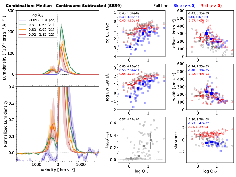
Figure 11: The influence of the [O iii]/[O ii] (O₃₂) ratio on the emergent Ly$\alpha$ line profiles. The left two panels show combined spectra in velocity space, stacked into four equally sized bins sorted by O₃₂ and median-combined. The upper panel shows the absolute luminosity density, and the lower shows the spectra when normalized by the luminosity red-wards of line centre to highlight variations in blueshifted emission. Values of O₃₂ that define the bin edges are given in the caption. The $2\times 3$ panels to the right show correlation diagrams. Quantities derived for the whole line profile are shown in grey, and the blue (red) points show the contribution from emission at negative (positive) velocities. In the six figures, we show the quantities of $f_{\mathrm{esc}}^{\mathrm{Ly}\alpha}$ and $W_{\mathrm{Ly}\alpha}$ at upper-left and centre-left respectively, and the lowest left plot shows the $L_{\mathrm{B/R}}$ ratio. The right-most column shows the higher order moments: velocity offset (moment 1), width (moment 2), and the skewness (moment 3). Kendall’s $\tau$ coefficient is written into each figure, together with the corresponding $p$-value. Solid points with errorbars correspond to the stacked profiles shown in the spectra to the far left.

In Figure 11 we show an example of the main correlation studies presented in this paper. This illustration shows the O₃₂ ratio ([O iii]/[O ii]), which is shown to be a strong correlate of the ionization parameter. The figure is divided into eight sub-figures: the left half illustrates the average line profiles as a function of the independent variable, derived by stacking analysis. Solid lines show the median stacked spectra, and shaded regions show the interquartile range (25–75 percentiles) calculated by bootstrap analysis. Many similar figures concerning other quantities may be found in the supplementary online-only materials.

Several trends become clear from Figure 11. Attending to the normalized stacked spectrum (lower left), the blueshifted emission provides a successively greater contribution to the total emergent Ly$\alpha$ at higher values of O₃₂. At the lowest values of O₃₂ $\approx 0.3$, Ly$\alpha$ absorption is visible at negative velocities, as more continuum radiation is absorbed in the Ly$\alpha$ resonance than is emitted by the nebular gas. Despite absorbing Ly$\alpha$, these galaxies remain in the sample because they are net Ly$\alpha$-emitters. The contribution of blueshifted emission then increases to $\gtrsim 30$ % at O₃₂ $\approx 10$. Across the same range of O₃₂, the redshifted component of the emission becomes narrower, which is most easily seen at a normalized flux density of about 0.1, where the red edge of the line profile recedes from $\sim 600$ to $\sim 400$ km s^-1.

The $2\times 3$ grid of plots to the right of Figure 11 shows how the O₃₂ ratio influences the global Ly$\alpha$ output. Grey points show the total $f_{\mathrm{esc}}^{\mathrm{Ly}\alpha}$ and EW, derived over the full 2500 km s^-1 window, and include both redshifted and blue-shifted emission. Blue (red) points show the same quantities, but calculated only for emission at $\Delta v<0$ ($\Delta v>0$), respectively, and can be thought of as the contribution to these frequencies to the total output. Kendall’s $\tau$ coefficient – a non-parametric rank statistic testing dependence between two variables – is calculated for the each of the figures, and written into the upper left corner of each subplot. The corresponding $p$-value is written immediately below. Firstly, and most obviously, there is a strong trend for the total escape fraction ($f_{\mathrm{esc}}^{\mathrm{Ly}\alpha}$) and EW to increase with the O₃₂ ratio, which spans more than an order of magnitude on both axes. In this example, the total $f_{\mathrm{esc}}^{\mathrm{Ly}\alpha}$ (black) relation is significant at $p\approx 10^{-9}$, and the EW relation is significant at $p\approx 10^{-15}$.

Notably in this example, there are equally strong relationships in place that describe the respective contribution of blue- and red-shifted emission. The red points closely trace the grey ones, which is natural because the red peak almost invariably dominates the total Ly$\alpha$. The less expected result is that not only does the blue-shifted emission correlate as strongly, but the slope of these correlations is steeper than those for the redshifted emission, and spans a factor of five greater dynamic range: the blue part of the Ly$\alpha$ profile is more sensitive to ionization conditions than the red part.

The lowest panel of the left column addresses the relative contribution of the blue and red peaks directly, by showing the dependence of the $L_{\mathrm{B/R}}$ ratio on O₃₂. In line with the more rapidly increasing EW of the blue-shifted emission, the $L_{\mathrm{B/R}}$ ratio increases sharply from effectively zero at an average O₃₂ of $\approx 1$, to $L_{\mathrm{B/R}}$ $\approx 0.35$ at O₃₂ $\approx 10$.

The right-most column shows various kinematic properties measured on the Ly$\alpha$ profiles, by the Lyman Alpha Spectral Database (Runnholm et al., 2021). In descending order we show the variation on higher order moments, 1, 2, and 3: velocity offset, line width, and skewness. Again they are computed for the full line profile (black), emission bluewards of line centre (blue) and red-wards (red). We note here that for the left column, where Ly$\alpha$ variables are derived from moment 0 (i.e. by numerical integrations), that it is not necessary to identify a clear peak: the integral is meaningful if the emission is not isolated to a peak. Higher order moments (offset, width, and skewness), however, demand the emission be peaked. The right-hand column, therefore, only shows data-points where peaks have been clearly detected – grey points and red points will be defined for the overwhelming majority of galaxies, but blue peaks are not ubiquitous, and there are fewer blue points than than red or grey. We use the peak-finding algorithm of Runnholm et al. (2021), which requires a (usually second) flux maximum be found at velocities in the range $-1000<\Delta v<0$  km s^-1, and that this be identified in $>95$ % of the Monte Carlo realizations. We also show the absolute value of velocity offset of the blue peak, in order to contrast the blue and points on the same axes; this can still be thought of as the distance between the peak and zero velocity.

The trends concerning the higher order moments are not as strong as those related to fluxes, but a number of interesting features still become apparent. There is a trend for the Ly$\alpha$ centroid shift to decrease with increasing O₃₂ (upper right). This trend is identified for both the total and red components, but is equally strong for the offset of the blue-shifted emission: for the highest three bins in O₃₂ the blue and red-peak offsets mirror each other. A very similar result is seen for the second moment, where both blue and red peaks become narrower with increasing O₃₂ (centre right subpanel). The lower right plot shows that only weak trends in skewness can be identified for the individual peaks, and their overall symmetry is not strongly dependent on the ionization conditions. The skewness of the total Ly$\alpha$, however, becomes systematically more negative as O₃₂ increases, because of the increasing contribution of the weaker blueshifted emission.

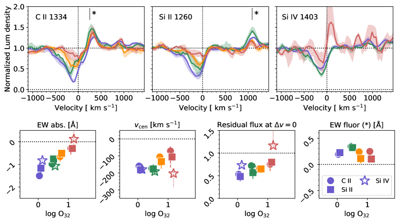
Figure 12: The influence of the [O iii]/[O ii] (O₃₂) ratio on the UV absorption lines. We show the C ii$\lambda 1334$Å, Si ii$\lambda 1260$, and Si iv$\lambda 1403$ Å lines in the upper row from left to right. Spectra are normalized to 1 in the continuum, and binning and color-coding are the same as Figure 11. Dotted vertical lines show systemic velocity of each line, and for the C ii and Si ii features we also indicate the velocity of fluorescent fine-structure transition with a star. The lower panels show measurements of various sample-averaged properties measured in the above stacks, and contrast them against O₃₂ – from left to right we show: the equivalent width of the absorption line; the centroid velocity of the absorption line (first moment); the residual intensity at zero velocity (the relative intensity at which an absorption feature crosses $v=0$); and the equivalent width of the fluorescent emission line (C ii and Si ii only). The color coding is the same in both rows, and also matches stacks in Figure 11. In the lower panels the absorbing species is encoded by different symbols (caption in the lower right panel).

6.1.2 Lessons from Ultraviolet Absorption Lines

The results presented in Section 6.1.1 show how various tracers of the Ly$\alpha$ output vary with a flux ratio in optical emission lines. Whatever the underlying physics is, it influences both total Ly$\alpha$ output (luminosity), relative output (EW and $f_{\mathrm{esc}}^{\mathrm{Ly}\alpha}$), and kinematics of the line profile (velocity offset and width). However this investigation itself does not point towards a causal mechanism; to bring our analysis one step closer to this we also examine the UV absorption lines, which we show in Figure 12.

The upper row is comparable to the left panels of Figure 11, and the galaxies entering each sub-stack are the same in both figures. Again, solid lines show the median stacked spectra, and shaded regions show the interquartile range. Attending first to the C ii absorption (left-most), the color sequence makes the opposite pattern that seen in Figure 11: the absorption becomes weaker as the O₃₂ ratio increases. The same effect can be seen in the Si ii absorption line, shown in the central panel of the upper row. In the rightmost plot we present the same analysis for the highly ionized gas using the Si iv$\lambda 1403$ Å line. This feature does not display such a clear trend with O₃₂, but it is noteworthy that the absorption almost vanishes for the highest O₃₂ bin. In fact, the net EW becomes slightly positive in this bin.

To better quantify these trends, we also compute the absorption EW, velocity centroid, and zero-velocity flux of each of the sub-stacks, and plot them against the independent variable in the lower panel. The decreasing absorption with O₃₂ can clearly be visualized, as the low ionization absorption lines exhibit EWs of $\approx 1.3$ Å for O₃₂ $\approx 1$, but fading to 0.4 Å at the highest O₃₂.

The centre left panel shows the first moment of the absorption line, which should trace the velocity of the (mostly outflowing) gas in front of the hottest (UV-brightest) stars. Average outflow velocities range from $\approx-250$ km s^-1, which is quite normal for compact starburst galaxies (e.g. Rivera-Thorsen et al., 2015; Henry et al., 2015; Heckman et al., 2015; Heckman & Borthakur, 2016; Chisholm et al., 2017, some of the galaxies in whose studies overlap with ours). In this example there is a modest trend for galaxies with more gas covering the stars to show faster outflows. Concerning Ly$\alpha$ emission, the faster outflows would accelerate more absorbing material away from the Ly$\alpha$ resonance and enhance the Ly$\alpha$ emission. However, it is also clear that despite the outflows being slower in the more highly ionized galaxies, there is also less gas covering overall.

To address this last point, the third lower panel shows the normalized residual flux density at zero velocity. The C ii and Si ii species in this figure very clearly correlate with O₃₂: higher ionization states in the ISM clearly imply less absorbing material close to line centre. It is impossible for Ly$\alpha$ to avoid scattering in this static material, and the amount (especially the column density) is responsible for splitting the intrinsic Ly$\alpha$ feature into double peaks.

Finally we draw attention to the fluorescent transitions associated with the C ii and Si ii absorption features. These result from the split ground-state (${}^{2}P^{0}_{J}$, where $J=1/2$ or $3/2$), and manifest as an emission line red-wards (slightly lower energy) of the main (resonant) transition. These are illustrated by the dotted vertical line at $\Delta v\approx 250$ km s^-1 for C ii and $\approx 1000$ km s^-1 for Si ii in Figure 12. These fluorescent transitions (which have been studied in detail by, e.g. Jaskot & Oey 2014; Scarlata & Panagia 2015; Carr et al. 2018) are detected at high significance in all of the sub-stacks presented for O₃₂. This C⁺ and Si⁺ exists within the COS aperture and is excited in the same transition by which the main lines are absorbed. However, as the strength of these emission components does not differ substantially with the strongly varying absorption, it appears the emitting and absorbing gas is not the same. We will return to this point in Section 7.3.

6.2 More Variables

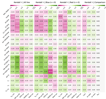
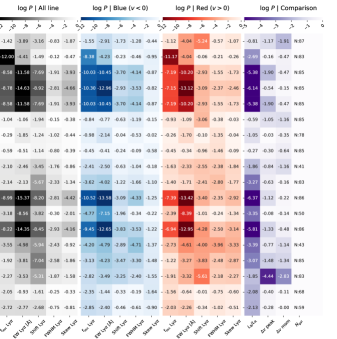
Figure 13: Heatmap showing strength and significance of relationships calculated between Ly$\alpha$ quantities ($x$-direction) and properties of the nebular gas ($y$-direction). The figure is divided in half, with Kendall’s $\tau$ shown to the left, and the associated $p$-value to the right. $\tau$ and $p$ are written into each cell. For $\tau$, the diverging colorbar is symmetric around zero and spans the range from –1 to +1, while $p$ is shown in logarithmic scale with the range showed by the colorbar. Each heatmap is divided into four groups in the $x$-direction, which are color-coded for the $p$-values: the first block of five shows coefficients for the quantities measured over the full line, including both blue-shifted and redshifted emission (i.e. derived from grey data points in Figure 11). The next two blocks show Ly$\alpha$ quantities computed only for the blue- and red-shifted emission, respectively (i.e. derived from the blue and red data points in Figure 11). The final block shows the same correlation coefficients for relative quantities computed between the blue-shifted and redshifted emission. In order: the $L_{\mathrm{B/R}}$ ratio, the velocity shift between the peaks, and the shift between the moments. The number of galaxies entering the correlation are shown in the final column.

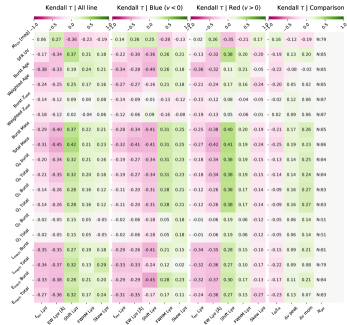
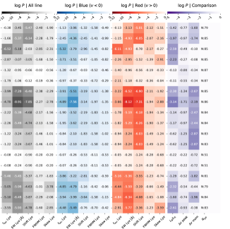
Figure 14: Heatmaps for Kendall’s $\tau$ and $p$ for properties derived from stellar population modeling. Caption the same as for Figure 13.

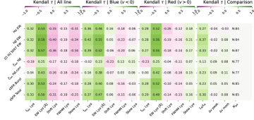
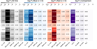
Figure 15: Heatmaps for Kendall’s $\tau$ and $p$ for properties derived from information that combines stellar and nebular modeling. Caption the same as for Figure 13.

Given the number of quantities we wish to investigate, and the wealth of information in Figures 11 and 12, we distribute the equivalent figures as online-only material. For other independent variables, we present the results as a series of heatmaps that record the Kendall $\tau$ coefficient and $p$-value. Figure 13 shows these heatmaps for the purely nebular properties, which we discuss first. In each cell we color code $\tau$ on a diverging color-scale between $-1$ and $+1$, where strong positive correlations are dark green, and strong anti-correlations are dark pink. The $p$-values are encoded on black, blue, and red colormaps to correspond to total, blueshifted, and redshifted Ly$\alpha$ for consistency with Figure 11. In each cell we also record $\tau$ (left group) and $p$ (right group) for quantitative use by the reader. Figure 14 shows the corresponding heatmaps for properties derived from stellar modeling, and Figure 15 shows quantities that are derived from combinations of stellar and nebular measurements.

Rows in the heatmaps (Figure 13) are grouped in approximate order by independent variables. First come variables associated with abundance: we show the H$\alpha$/H$\beta$ ratio, which scales with dust reddening, and the N2 and S2 indices that roughly encode the abundance of nitrogen and sulphur ions relative to hydrogen. Then come a number of variables that should scale with the ionization state: these include recombination line variables at the top (e.g. He i/H$\beta$ and He ii/H$\beta$), followed by metal ions relative to hydrogen (e.g. [Ar iii]/H$\alpha$), followed by metal line ratios such as [O iii]/[O ii] (already discussed in Section 6.1.1 and Figures 11 and 12), [Ne iii]/[O ii], etc. Finally towards the bottom of the figure we show the influence of thermodynamic variables: temperature, density, and pressure.

In terms of the dependent variables, we include the majority of the Ly$\alpha$ variables discussed in Figure 11. The x-direction of the heatmap is divided into four groups: the first shows Ly$\alpha$ quantities computed over the entire line profile, comprising both negative and positive velocities (corresponding to grey/black points in Figure 11). We show $f_{\mathrm{esc}}^{\mathrm{Ly}\alpha}$, the Ly$\alpha$ EW, and the first, second, and third moments. The second block shows these same quantities computed over negative velocities only (blue points in Figure 11), and the third for positive velocities (red points in Figure 11). The final block shows correlations regarding direct comparisons between blue and red emission: the first is the blue/red flux ratio, the second is the distance between the peaks in velocity space, given by peak identification (first) and moment calculation (second). Finally, in the last column, we show the number of data-points from which each correlation is calculated.

Figure 14 proceeds in the same fashion. From top to bottom we show stellar properties of age, which is further divided into starburst age and mass-weighted total age, followed by abundance (similarly divided), and mass (divided into burst and total). Then follow ionizing photon production rates (for H, He⁰, and He⁺), and mechanical luminosities and integrated energies, all of which are shown for both starburst and total components.

Figure 15 shows quantities combining nebular and stellar estimates. We first show equivalent widths, which encode the intensity of line radiation in comparison to the underlying stellar radiation at the same wavelength. This most strongly scales with the specific star formation rate or recent evolutionary history, depending upon wavelength. To tease out these contributions we also examine the ionizing photon production efficiency ($\xi_{\mathrm{ion}}$), which we derive from the dust-corrected H$\beta$ luminosity, and the specific SFR for which we adopt the stellar masses of both the burst and total population.

7 Main empirical findings

We begin by presenting a summary of our main findings, which concern how observables that trace differing physical processes influence the Ly$\alpha$ output, its shape, and the behaviour of the ISM absorption lines. We then proceed to discuss the Ly$\alpha$ kinematic properties and inferences made from the fluorescent lines of C ii and Si ii.

7.1 Lyman alpha Output and LIS Absorption with Respect to Conditions

7.1.1 Evolutionary Phase of the Starburst

Given the dependence of Ly$\alpha$ production on the photoionization rate, and the implication of stellar feedback in ionizing and clearing the ISM, it is unavoidable that stellar age must have a significant effect on the Ly$\alpha$ output. We have several tracers of age, that stem directly from spectral modeling (Sect 3.1), and from the nebular response in terms of the EW of hydrogen and helium recombination lines.

Stellar ages show strong anti-correlations with $W_{\mathrm{Ly}\alpha}$, which decreases by a factor of $\sim 10$ (roughly from 100 Å to 10 Å over the 1–10 Myr timescale. The trend is more significant when the starburst age is considered, removing the contamination from more evolved stars that no longer contribute to photoionization: $\tau$ increases from $\sim 0.25$ to $\sim 0.4$ and $p$ drops from $\sim 10^{-3}$ to $\sim 10^{-6}$. This is entirely expected from the perspective of Ly$\alpha$ production, and similar results are shown for the EW of H$\beta$ in Figure 8. It is less obvious that $f_{\mathrm{esc}}^{\mathrm{Ly}\alpha}$ should behave similarly, since $f_{\mathrm{esc}}^{\mathrm{Ly}\alpha}$ is not directly causally related to the intrinsic Ly$\alpha$ luminosity. However, $f_{\mathrm{esc}}^{\mathrm{Ly}\alpha}$ also anti-correlates with the stellar age and with similar dynamic range and significance, which implies two things. Firstly, $f_{\mathrm{esc}}^{\mathrm{Ly}\alpha}$ must be connected to the age by a hidden third variable, such as increased dust production or the loading of the winds with cool material. Secondly, the trends of $W_{\mathrm{Ly}\alpha}$ and age are not purely related to intrinsic Ly$\alpha$ production but must also be modulated by these transfer effects. It is interesting that when we study the ionizing photon production efficiency ($\xi_{\mathrm{ion}}$) directly that the trends with $W_{\mathrm{Ly}\alpha}$ remain, but $f_{\mathrm{esc}}^{\mathrm{Ly}\alpha}$ almost vanish.

An almost identical picture is revealed by the Balmer line EWs, but the significance is improved and $\tau$ reaches 0.6 with $p\approx 10^{-15}$ for the relation between $W_{\mathrm{Ly}\alpha}$ and $W_{\mathrm{H}\beta}$. This is naturally expected since both the EWs intrinsically reflect the number of ionizing photons compared to the underlying stellar light. However the almost-as-strong correlations concerning $f_{\mathrm{esc}}^{\mathrm{Ly}\alpha}$ ($p\approx 10^{-5}$ for $W_{\mathrm{H}\beta}$) clearly demonstrate that the escape of Ly$\alpha$ is also heavily modulated. This correlation is stronger for $W_{\mathrm{H}\beta}$ than for $W_{\mathrm{H}\alpha}$ because of the smaller wavelength difference between Ly$\alpha$ and H$\beta$, which is less contaminated by underlying, older stellar generations than H$\alpha$.

A partial explanation for the escape fraction behaviour is demonstrated by the evolution of the LIS absorption in the stacked UV continuum spectra: with $W_{\mathrm{H}\beta}$ increasing from $\sim 30$ Å to 300 Å, the EW of absorbing gas decreases by a factor of four in the C ii $\lambda 1334$Å absorption line ($-1.6$ to $-0.4$ Å). This traces a decrease in the combined effects of covering fraction and column density of cool gas, which absorb the Ly$\alpha$.

An interesting observation is how the absorption EW of C ii and Si ii increase with age (and decreasing Balmer EW). We argue this results from an increasing loading of the wind with time as it is accelerated. It is clear also that the velocity offsets are smallest ($\lesssim 100$ km s^-1) when the starburst is youngest, but then increase by a factor of about two. The individual UV spectra are not sufficiently deep for us to robustly derive outflow masses, mass-loading factors, etc. for each galaxy. Indeed, it is for this reason that we resort to stacking analyses for UV absorption line measurements. However, we studied these quantities in detail in Hayes (2023) in exactly the same dataset, using the same sub-bins for stacking. In that paper we showed that the covering of cool gas, and consequently the outflow rate and mass loading factors increase over the duration of the starburst episode. Wind masses grow from $\sim 10^{4}-10^{8}$ M_⊙ over the 1–10 Myr duration, which could either be because it takes time to accelerate cool gas or advect it into the flow, or for cooler absorbing material to condense out of the warmer outflowing gas. In either scenario, the column of Ly$\alpha$-absorbing column increases with time, which would contribute to the negative relationship between both $W_{\mathrm{Ly}\alpha}$ and $f_{\mathrm{esc}}^{\mathrm{Ly}\alpha}$ with evolutionary independent variables.

We previously hypothesized that the Ly$\alpha$ output should be modulated by the amount of mechanical energy returned by feedback. Both $f_{\mathrm{esc}}^{\mathrm{Ly}\alpha}$ and $W_{\mathrm{Ly}\alpha}$ are strongly anti-correlated with the mechanical luminosity ($L_{\mathrm{mech}}$) and its total integral since the onset of the starburst ($E_{\mathrm{mech}}$). This relationship runs contrary to our hypothesis, in that more Ly$\alpha$ is emitted when less mechanical energy is available (or has been deposited). This relationship is attributed to second order effects, and may indicate that while this feedback must be responsible for accelerating large scale winds, it is sub-dominant to other processes when considering the emission of Ly$\alpha$ (see Section 7.1.3).

As discussed in Section 6.1.1 the total Ly$\alpha$ output is dominated by the redshifted component, as shown by the alignment of grey and red data-points in the $f_{\mathrm{esc}}^{\mathrm{Ly}\alpha}$ and $W_{\mathrm{Ly}\alpha}$ figures. However the slope of the points for the blue-shifted emission rises more steeply, and the blue-shifted emission contributes more at larger $W_{\mathrm{H}\beta}$. The fraction of blue-shifted emission, $L_{\mathrm{B/R}}$, is shown directly, which rises from effectively zero at $W_{\mathrm{H}\beta}$ $\approx 30$ Å to 0.3 at $W_{\mathrm{H}\beta}$ $\approx 300$ Å ($p\approx 10^{-6}$). This rapid increase requires a decreasing column densities of gas at negative velocities, which is supported once more by the absorption lines: not only is there less absorption in total at higher $W_{\mathrm{H}\beta}$, but the level of absorption at zero velocity also falls by a factor of $\approx 2$.

The basic interpretation for the above is that evolutionary stage modulates the Ly$\alpha$ output, both by affecting the intrinsic Ly$\alpha$ production and its transfer. A working scenario is one in which the abundance of ionizing photons at smaller ages also leads to higher ionization gas, and less cool absorbing material – this would also be consistent with the decreasing C ii and Si ii at higher $W_{\mathrm{H}\beta}$. In other words, that in terms of Ly$\alpha$ the ‘rich get richer’, i.e., since ionizing photons not only increase the intrinsic emissivity is increased but also the escape is facilitated (Kakiichi & Gronke, 2021). The same effect on the LIS lines can also be explained by the changing the ISM abundances of carbon and silicon, which is the subject of the next subsection.

7.1.2 Abundances of Dust and Metals

We use the H$\alpha$/H$\beta$ ratio (or H$\gamma$/H$\beta$ where H$\alpha$ is clipped) to estimate the dust obscuration, and the ratios of [N ii]6584/H$\alpha$ (N2), [S ii](6717+6731)/H$\alpha$ (S2) indices as proxies for the nebular metallicity (e.g. Pettini & Pagel, 2004; Marino et al., 2013; Kewley & Dopita, 2002; Yin et al., 2007).

The absolute Ly$\alpha$ output (both $f_{\mathrm{esc}}^{\mathrm{Ly}\alpha}$ and $W_{\mathrm{Ly}\alpha}$) strongly anti-correlate with the dust obscuration in way that are both intuitive and have been shown before (Scarlata et al., 2009; Hayes et al., 2010, 2014; Atek et al., 2009; Atek et al., 2014). This is also very clear when comparing the H$\alpha$/H$\beta$ ratios with the LIS absorption lines, which shows that the covering gas also reddens the light (e.g. Shapley et al., 2003; Gazagnes et al., 2018). It is apparent that sorting the sample by dust obscuration also sorts by the amount of absorbing gas at $\Delta v=0$: the least dusty galaxies show almost no absorption at zero velocity, which is probably responsible for the downwards trend in $L_{\mathrm{B/R}}$ with H$\alpha$/H$\beta$.

While the above relations are quite intuitive, it is not clear whether H$\alpha$/H$\beta$ stacking sorts the sample along an age sequence (both dust production and destruction/clearing scenarios could be envisaged). Outflow velocities are smaller in more obscured galaxies, firstly suggesting that radiation pressure on dust grains is not a significant accelerator of winds (or that the trend is otherwise obscured). A plausible explanation is that dustier winds are more massive and more energy is required to accelerate the gas.

The effects with nebular metal abundances (traced by N2 and S2 indices) assist in the interpretation: the anti-correlation of these quantities with Ly$\alpha$ output are stronger than those for H$\alpha$/H$\beta$, with $p\approx 10^{-15}$ for S2 vs. $W_{\mathrm{Ly}\alpha}$ and $p\approx 10^{-9}$ for $f_{\mathrm{esc}}^{\mathrm{Ly}\alpha}$. Abundances can explain this in two ways: by lower metallicity stars having higher ionizing photon production, and by more metals producing more dust to obscure the emitted Ly$\alpha$. The EW of LIS absorption lines is also strongly correlated with the S2 index, where more nebular [S ii] emission aligns with more interstellar absorption. This could be the result of ISM abundances and it is curious that, for example, the Si ii EW varies by a factor of $\approx 8$ while the S2 index changes by a similar amount, which would imply close-to constant gas hydrogen if metallicity were the only action. (Note, however, that metallicity calibrations using strong lines are seldom linear with the index.) Almost constant hydrogen columns would not cause major differences to the Ly$\alpha$ output, which changes significantly, and by larger factors than the LIS absorption. This would argue that the ISM lines are saturated and the trend with H i covering is in fact significant.

Here we may use the expected correlation between abundances in the ISM and the stars. Lower metallicity stars experience less photospheric opacity from metal absorption, and produce more ionizing photons at fixed mass; this increases the Ly$\alpha$ production (intrinsic EW) and also produces a more highly ionized ISM and increases the Ly$\alpha$ transmission. However we see no noticeable influence of stellar abundance on the observable Ly$\alpha$ properties ($p\gtrsim 0.05$), implying that this effect is likely not an important driver of either Ly$\alpha$ production or, by secondary effect, emission.

A further interesting point is that when testing nebular metallicity as an independent variable, we again recover the strong evolution of the $L_{\mathrm{B/R}}$ ratio, which peaks at at $\approx 0.4$ for the least metallic galaxies. There is no case for this unless the amount of absorbing material close to zero velocity is not strongly correlated with the metallicity, which would further argue for ionization levels to be the main driver.

A final point of interest is that the S2 index correlates more tightly with Ly$\alpha$ variables than the N2 index. N2, however, is the preferred measure of metallicity, which suggests there may be confounding factors. Because S⁺ forms in the partially neutral medium (I.P. range: 10.4–23.3 eV) but N2 does not (14.5–29.6 eV), an extra deficiency factor for S2 may result when the ISM becomes highly ionized (Wang et al., 2019). The [S ii] deficit (Section 3.2.2) encodes the lack of [S ii] emission at fixed metallicity, and has been argued as a tracer of low optical depths to ionizing photons. When we contrast the Ly$\alpha$ output against $\Delta$[S ii] we see weaker but significant trends ($p\approx 10^{-4}$) for Ly$\alpha$ to be stronger when the deficit is larger, lending weight to the use of this variable to segregate between galaxies where the hydrogen optical depth is low (see Wang et al., 2021).

7.1.3 Ionization State

Without a detailed photoionization model, we do not have direct estimates of the ionization state of the gas. However many line ratios are available, and the nebular lines measured in this paper trace species ionized by photons with energies between $\approx 11$ eV at the low ionization end, up to 54 eV at the high end. Ratios of some of these are often invoked as indicators of the ionization level of the nebular gas, although like with abundances there are many caveats to single line ratios.

This has already been discussed in Section 6, where we focussed upon the O₃₂ ratio, but Figure 13 shows many line ratios. We sort these by ratios of pure recombination lines (RL; e.g. He i/H$\beta$ and He ii/H$\beta$), followed by ratios of collisionally excited lines (CEL) to RL, (e.g. [Ar iii]/H$\alpha$, [Ar iv]/H$\beta$), and then ratios involving collisional lines only (e.g. [Ne iii]/[O ii], [O iii]/[O i], and [Ar iv]/[Ar iii]).

Beginning with the RL ratios, effectively no trends are seen when using the He i 5876/H$\beta$ ratio, implying the ratio does not separate out physical properties that influence Ly$\alpha$ emission. (There is a trend for higher He i/H$\beta$ ratios to show both thicker and faster outflows, but currently we do not have an explanation for this.) The lack of correlation with Ly$\alpha$ probably indicates that in all these galaxies, the helium-ionizing photon production rate ($Q_{1}$) is a sufficient fraction of $Q_{0}$ ($Q_{1}/Q_{0}\gtrsim 0.15$; Draine 2011) that the H⁺ and He⁺ Strömgren spheres are bound together and the line ratio contains little diagnostic information.

One may expect the He ii line to provide more diagnostic power than He i, as the requirement of a significant photoionization rate at energies above 54 eV must identify the hottest stars. In a sample of $z\approx 2$ galaxies identified by Matthee et al. (2021), it was later shown that the higher EW LAEs, and galaxies with more blueshifted emission, did indeed show higher He ii/H$\beta$ ratios (Naidu et al., 2022). In this context, our result is surprising: the Ly$\alpha$ output is not significantly correlated with He ii/H$\beta$. A similar result has already been obtained for the LyC output of starburst galaxies (Marques-Chaves et al., 2022), who argue variations in this line ratio are driven mainly by metallicity; having addressed abundances in Section 7.1.2 it is surprising we do not see the secondary correlation here. A possibility is that because the He²⁺ zone is small, it does not contain much information regarding the environments where Ly$\alpha$ is absorbed, but the same could be argued for [Ar iv], [Ne iii] and even [O iii]. Another alternative is that He ii is produced by processes other than photoionization, such as fast radiative shocks. This could also explain a lot of the difficulty experienced in reproducing the He ii fluxes with pure photoionization models (Kehrig et al., 2018; Senchyna et al., 2020; Olivier et al., 2021; Wofford et al., 2021).

Moving to the CEL/RL ratios, [Ar iii]/H$\alpha$ and [Ar iv]/H$\beta$ both show weak but significant trends with Ly$\alpha$ output behave in opposite directions. [Ar iii]/H$\alpha$ anti-correlates with $W_{\mathrm{Ly}\alpha}$ and $f_{\mathrm{esc}}^{\mathrm{Ly}\alpha}$, while [Ar iv]/H$\beta$ positively correlates ($p\approx 0.005$ typically). It appears that the [Ar iii]/H$\alpha$ ratio is more closely aligned with the metallicity, which produces the trend on this variable, and indeed the same [Ar iii] line has been proposed as an abundance diagnostic, albeit with a different denominator (Stasińska, 2006). Ly$\alpha$ output increase for higher fluxes in the higher ionization potential [Ar iv] lines (40–60 eV). Ly$\alpha$ also becomes bluer at high [Ar iv]/H$\beta$, and the LIS absorption becomes weaker, with behaviour similar to the O₃₂ diagnostic discussed previously. The faintness of the [Ar iv] doublet, however, reduces our sample, and we cannot afford the same number of bins as for stronger lines.

Pure CEL ratios far surpass ratios involving recombination lines in predicting Ly$\alpha$ output, as demonstrated with O₃₂ in Section 6.1. Abundance variations cannot be the cause, because ratios of comparable ionization potential to hydrogen (e.g. N2 and S2; Section 7.1.2) also out-perform higher potential ratios like those of [Ar iii] and [Ar iv] above. The commonplace O₃₂ and Ne3O2 indices (Levesque & Richardson, 2014) are the best-predictors in our study, with $\tau\gtrsim 0.6$ ($p\sim 10^{-15}$) against global Ly$\alpha$ metrics in both cases. This is partly intuitive as abundance variations can have zero influence in the case of O₃₂, and very little influence for Ne3O2 since neon is produced in the same way as most oxygen, with the addition of one extra alpha particle. Similar results are obtained for the [O iii]/[O i] ratio (O₃₁) ratio although the trend is weaker.

It is important to point out that the EW of LIS absorption features strongly correlates with O₃₂ and Ne3O2 indices. We discussed a similar trend with abundance in Section 7.1.2, but noted that if abundance scaled directly with N2 and S2 ratios, then variations in the absorption EWs of Si ii and C ii could actually point to fixed hydrogen column. That the same LIS absorption EWs also vary strongly with O₃₂ show that this cannot be the case as this intensity must also modulate the ionization correction factors, and amount of H traced by C⁺. The ionization state must be increased for the extreme O₃₂ galaxies, pushing more of the carbon into the C²⁺ state.

Further support for this comes from the argon lines, whose predictive power is increased when combined with each-other. This is observationally remarkable given the relatively shallow nature of SDSS spectra, and the fact that these lines are $\approx 100\times$ weaker than the strong oxygen lines. The [Ar iv]/[Ar iii] ratio (Ar43) also strongly correlates with $L_{\mathrm{B/R}}$ and with the UV absorption lines, revealing similar traits to O₃₂ at somewhat higher potential. Both the C ii and Si ii lines almost vanish in the highest Ar43 bin, and even at $\Delta v=0$ the stack shows little absorption (residual intensity of $\approx 80$ % in Si ii and C ii. It appears that galaxies with the strongest [Ar iv] emission are fully ionized, explaining the low column densities of absorbing material, and the large contribution of blueshifted Ly$\alpha$ emission.

7.1.4 Thermodynamic Variables

Finally we draw attention to some quantifiable physical conditions in the ISM: those of temperature, density, and pressure. These are inferred from variations in the ratios of (often) weak emission lines: the 6717/6731 Å doublet of [S ii] for the electron density ($n_{\mathrm{e}}$), and the 5007/4363 Å ratio of [O iii] for temperature ($T_{\mathrm{e}}$). The product of these two quantities is the pressure ($P_{\mathrm{e}}$), although note that $P_{\mathrm{e}}$ and $n_{\mathrm{e}}$ are almost equivalent as variables because the dynamic range of $n_{\mathrm{e}}$ far exceeds that of $T_{\mathrm{e}}$. One may intuitively expect these variables to rank as important correlates in this study, as they are direct assessments of physical conditions.

Weak correlations exist between all of these variables and $W_{\mathrm{Ly}\alpha}$ and $f_{\mathrm{esc}}^{\mathrm{Ly}\alpha}$, in the direction that Ly$\alpha$ is stronger at higher temperature and density. However these are weaker than for many other variables, with $\tau\sim 0.2$ and $p\sim 10^{-3}$ for the sample. Some suggestive relationships can be seen when examining the LIS absorption lines. Specifically, the absorption EW is correlated with ISM temperature, in the direction that hotter galaxies show less absorption – the most likely explanation is that the galaxies with hotter ISM are also more highly ionized, lowering column densities in the lower ionization C⁺ and Si⁺ stages. Also the outflow velocities of the gas increase dramatically –by a factor of 3– with ISM density and pressure (regardless of $T_{\mathrm{e}}$). In itself this is also intuitive because more pressurized environments should accelerate the surrounding gas more rapidly; it is not intuitive, however, why these effects of $T_{\mathrm{e}}$, $n_{\mathrm{e}}$, and $P_{\mathrm{e}}$ do not affect the Ly$\alpha$ output. Sorting on these variables does not uniquely sort by Ly$\alpha$ observables, and we speculate that these thermodynamic variables may be useful to follow up as independent variables.

7.1.5 An Underlying Effect of Stellar Mass?

After discussing many variables tracing ISM conditions, the remaining question is that of galaxy mass. Is this the factor that governs everything else by secondary correlation? Figure 10 shows there is an anti-correlation between $W_{\mathrm{Ly}\alpha}$ and stellar mass, and our heatmaps show this relationship to have $\tau\approx-0.4$ with $p\approx 10^{-9}$. Indeed stellar mass is a vital variable to consider. However the amplitude of variation of $f_{\mathrm{esc}}^{\mathrm{Ly}\alpha}$ with mass is comparable to that of $W_{\mathrm{Ly}\alpha}$, which implies the variations in EW are driven more by conditions in the ISM and not through those of the stars ($\xi_{\mathrm{ion}}$ or evolutionary phase).

Similar effects are seen in relationships between Ly$\alpha$ output and the FWHM of the optical emission lines, which would trace the total mass of the system under dynamically relaxed conditions. Both Ly$\alpha$ tracers do decrease with increasing FWHM and the absorption lines become stronger (suggestive of a mass sequence) but these trends are only marginally significant. We conclude that mass and intrinsic dynamics of the H ii regions are important in the emission of the Ly$\alpha$ radiation, but mainly by correlation with ISM-related properties.

7.2 Kinematic Properties of Lyman alpha

7.2.1 Velocity Shift and Width: Moments 1 and 2

In this section we discuss the influence of our independent variables on the higher order moments of the Ly$\alpha$ line: the velocity offset, width, and skewness. In this section we must be cautious, as these measurements may be influenced by varying contributions of the red and blueshifted components, instead of actual variations in any one of the two peaks. We discuss these possible effects following the same structure as above.

Evolutionary Stages of Star Formation

As indicated by the EW of Balmer lines and modeled age, evolutionary stage has a mild effect on the total Ly$\alpha$ kinematics. However in terms of offsets (moment 1), neither the blue nor red peaks are in themselves strongly affected by age estimators. The reason for the strong correlation in the total line (measured over a 2500 km s^-1 window) ($p\approx 10^{-7}$), is that the blue peak increases systematically in contribution with respect to the red peak ($L_{\mathrm{B/R}}$ increases strongly), which shifts the central moment closer to $\Delta v=0$. We do not see any strong or significant trends of the velocity width with the evolutionary stage variables (e.g. $L_{\mathrm{mech}}$, $E_{\mathrm{mech}}$).

Abundances of Dust and Metals

Ly$\alpha$ kinematic properties appear invariant with dust obscuration, but certainly not with metal abundance. The shift of moment 1 of the total line evolves in the same way as described above, because of changing $L_{\mathrm{B/R}}$. More interestingly, when contrasted with N2 and S2, the individual components are both systematically shifted away from line-centre in more metal rich systems: the amplitude of this effect runs from 200–300 km s^-1 and is significant at $p\approx 10^{-4}$. Trends of both comparable amplitude and significance are also visible in second moment. In summary, more of the Ly$\alpha$ emission is concentrated closer to line centre in less metallic galaxies.

Ionization State of the Gas

Clear kinematic trends are visible, and are strongest among the line ratios that have already been discussed as having the most influence over the global Ly$\alpha$ output (e.g. Section 7.1.3). Both the first and second moments strongly anti-correlate with ionization parameter, as probed by O₃₂ (Figure 11), Ne3O2 and also Ar43 (online-only materials).

Thermodynamic Variables

$n_{\mathrm{e}}$ and $P_{\mathrm{e}}$ do not separate galaxies into significantly different sub-groups by Ly$\alpha$ kinematics. Electron temperature, however, shows a remarkable trend of decreasing velocity offset (factor of 2, $p\approx 10^{-5}$) and width (similar amplitude, $p\approx 10^{-3}$). Even a posteriori it is difficult to explain this trend, but we speculate it may be coupled to the decline in absorbing column density with increasing temperature that we discuss in Section 7.1.4.

An Underlying Mass Effect?

The answer to this question is a resounding yes. Velocity offsets from line centre (moment 1) of the individual peaks are most strongly correlated with mass. The dynamic range in offset is about a factor of 2 (as above) but the $p$-value drops to $10^{-7}$ ($10^{-4}$) for the red (blue) peak. However, the bulk of this effect must be attributed to radiative transfer effects, and cannot be explained by a larger fraction of Ly$\alpha$ being emitted at greater velocity offsets (see Stark et al. 2017 and Mason et al. 2018 for further discussion). While it is absolutely the case that more massive galaxies have broader intrinsic optical lines, the trend between the FWHM of the optical features and Ly$\alpha$ moments is barely statistically significant.

As with the global Ly$\alpha$ output, tracers of metallicity and ionization parameter are best able to identify differences in Ly$\alpha$ offset and width. In contrast, the evolutionary tracers (ages and Balmer EWs) appear unable to sort galaxies this way. Both offsets and Ly$\alpha$ width are linked to radiative transfer effects, where a higher column density implies the need for larger frequency excursions at scattering: the effects concerning O/H and log $U$ could therefore be the result of a harder ionizing spectrum that ionizes more of the interstellar medium and reduces the overall column density and residual H i fraction.

In this context, it is interesting that we do not see the kinematic measurements evolve during the starburst event, or on timescales that can be probed with UV-optical spectroscopy. This is remarkable, since we do see strong evolution in the EW and first moments in the LIS absorption lines over these timescales. We suspect that the critical quantity in shaping the Ly$\alpha$ is the column density of gas close to zero velocity, which evolves much more slowly than either the EW or centroid velocity of the absorption. The fact there is an overall trend with total galaxy mass shows that the line profile will evolve on longer timescales as galaxies assemble, and this may also explain some of the above trends as secondary correlations. For example, less metallic galaxies are also less massive on average (e.g. Tremonti et al., 2004), which results in narrower intrinsic Ly$\alpha$ profiles as observed here; dust is also built up in starburst events, mixed, and accelerated to velocities where it may have varying effects on the line profile.

7.2.2 Skewness: Moment 3

The skewness of the total Ly$\alpha$ emission line was first derived (in slightly different forms) to distinguish between Ly$\alpha$-emitting galaxies and other single-line emitters in galaxy surveys (e.g. Rhoads et al., 2003; Shimasaku et al., 2006; Kashikawa et al., 2006). It has since been studied in more detail in both galaxies (U et al., 2015; Childs & Stanway, 2018) and extended Ly$\alpha$ halos (Herenz et al., 2020), and put forward as a diagnostic of scattering scenarios in different geometries (e.g. Remolina-Gutiérrez & Forero-Romero, 2019). Clearly the Ly$\alpha$ skewness must be connected to resonance scattering and modulated by kinematic effects that preferentially reshape one side.

We find the skewness of total Ly$\alpha$ line (measured over all velocities) to be most strongly connected with variables concerning stellar evolutionary state, ionization state, and nebular abundance (all with $p\approx 10^{-4}$), with a weaker but still significant effect seen in total mass ($p\approx 0.01$). However, as discussed at the top of Section 7.2.1, this effect is entirely one in which skewness become increasingly negative as the blue peak become systematically stronger. It does not relate to the earlier proposition of skewness in individual peaks that identify LAEs (e.g. Kashikawa et al., 2006) or investigate outflows (U et al., 2015).

We proceed to investigate the skewness of the red and blue components independently. In the blue peak we find significant relations (defined conventionally as $p<0.05$ between skewness and Ar43, $\Delta$[S ii], $T_{\mathrm{e}}$, $n_{\mathrm{e}}$ (but not their product, $P_{\mathrm{e}}$) and stellar mass. The lack of some correlations may be the result of relatively poor signal-to-noise in many of the blue peaks, and the lack of correlations with O₃₂ and Ne3O2 cast doubt upon the Ar43 relation. Indeed the red peak shows stronger relations with skewness, which increases (becomes more extended towards high velocities) at low metallicity, high ionization parameter, increasing deficit of [S ii] and higher temperature. Most of this appears connected to ages derived over longer timescales, as evidenced by an anti-correlation with total age and mass ($p\approx 10^{-3}$).

7.3 Fluorescent Emission Lines and Circumgalactic Gas

A prominent feature in some of the stacked UV spectra is the presence of the fluorescent emission lines arising from the split ground state of the C ii and Si ii transitions. These lines have been discussed for some time in connection with the circumgalactic gas content of galaxies: e.g. in low-$z$ Ly$\alpha$-emitting starburst KISSR 242 (a.k.a. LARS 07; France et al., 2010) and at $z\approx 3$ in the stacks of Lyman break galaxies (Shapley et al., 2003). They have also been used to estimate the 3-dimensional configuration of galaxy outflows in unresolved observations (Scarlata & Panagia, 2015; Carr et al., 2021). The overwhelming majority of this line emission is excited by absorption in the ${}^{2}P^{0}_{1/2}\rightarrow^{2}D_{1/2}$ (the resonance transition to the lower ground state) that then decays instead to the ${}^{2}P^{0}_{3/2}$, releasing a photon red-wards of the resonance. The key point is that gas emitting a fluorescent line must have absorbed in a resonance transition.

Our stacked spectra show clear fluorescent lines in both the C ii* and Si ii* species, with typical EWs of 0.2–0.3 Å. The Si ii* line (whose offset in velocity space is $\approx 1250$ km s^-1 from resonance) is well centered at the systemic velocity (determined by optical nebular lines). The peak of the C ii* line appears redshifted, but this is probably a result of blending with the absorption, as the intrinsic velocity difference is only 250 km s^-1. A key finding of this work is that, while the absorption EWs may vary by factors of 4–5 (e.g. with Ne3O2) the EW of the fluorescent line is invariant.

Aperture size will of course be important to capture all the fluorescent emission, but it is hard to envisage a scenario in which its EW does not correlate with the resonantly scattered Ly$\alpha$ line – we tested this explicitly with both Ly$\alpha$ luminosity and EW as the independent variable. Our interpretation is that the larger amounts of absorbing gas are actually due to a more extended halo – in this scenario the line-of-sight distance grows to provide a greater column density and deeper absorption. Since the galaxies with strongest absorption are also found to be more evolved, this would also support the scenario in which wind envelopes are built up successively with time (Hayes, 2023). At larger foreground distances, both scattering into the line of sight (‘resonant infilling’) and fluorescent emission towards the observer become successively less likely for geometric reasons. Thus the fluorescent line is dominated by emission from close to the star forming regions and does not vary with total column density.

8 Quantifying the scatter: multi-dimensional analysis of the relations

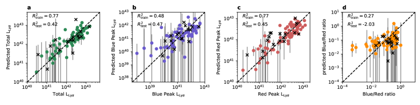
Figure 16: Predictions of the total, blue, and red luminosities as well as the ratio of the blue to red luminosity. The prediction is on the y-axis and the true measured value on x. Colored points indicate the training sample and black xs mark the test sample. $R^{2}$ values denoted in each panel show the coefficient of determination for the training and testing sample respectively.

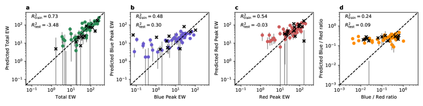
Figure 17: Predictions of the total, blue, and red EWs as well as the blue over red ratio. For details see caption of Figure 16

So far we have presented a large number of correlations between optical and UV line properties and Ly$\alpha$—some of which are unprecedentedly strong. In this Section we investigate whether we can use multi-parametric analysis to provide even stronger predictive relations for Ly$\alpha$. Similar analysis was done in Runnholm et al. (2020), with the aim of predicting global Ly$\alpha$ luminosities measured in narrowband imaging. With the quantities derived from the LASD we can expand upon this and test whether predictions can be made for the blue and red components of Ly$\alpha$ separately.

We start out by subdividing both our Ly$\alpha$ quantities and our predictors into two groups: luminosities and ratios. For the first group we want to predict the total, blue and red Ly$\alpha$ luminosities as well as the blue over red ratio using optical line luminosities. We selected the line luminosities to use as predictors by first filtering on signal-to-noise, requiring a median SNR of 10 across the sample of galaxies. We then curated this line list by manually removing lines with redundant information, for instance by including the sum of the [O ii]$\lambda\lambda 3726,3729$ Å doublet instead of the individual lines, leaving us with a total of nine lines.

For the second group we aim to predict the Ly$\alpha$ EW, again divided into total, blue, and red components. For this model we select a set of line ratios, or quantities derived from such based on each quasi-group presented in Section 3.2.2. The parameters we consider are: H$\beta$ EW indicating stellar evolutionary state, H$\alpha$/H$\beta$ ratio indicating dust, N2 index as a metallicity tracer, [Ne iii]/[O ii] as a marker of ionization state, [S ii] deficit as an indirect indicator of the neutral gas column, and the temperature and pressure measured from [O iii] and [S ii], respectively.

The model we use in both cases is a simple multivariate linear regression. We choose this model because it has a low number of free parameters and maintains a high level of interpretability. For the luminosity model we use a standardization that includes first taking the logarithm of the variables, and then performing a more ordinary standardization – subtracting the means and dividing by the standard deviations, often referred to as z-score standardization. This ensures that all variables are comparable but it should be noted that this means that the model in this case is a power law rather than linear. For the prediction of ratios we only use a z-score standardization. Standardizations and model fitting was done using the sklearn python package.

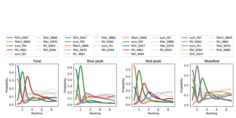
Figure 18: Variable importance for the luminosity predictions. On the x-axis is the variable ranking with 1 being the most important variable and 10 the least important. Each curve shows the distribution of rankings for one variable over the set of 2000 Monte Carlo iterations converted to a probability density function by a kernel density estimator with a Gaussian kernel of width $0.5$. The 4 most variables with the lowest mean rank are highlighted with thicker lines.

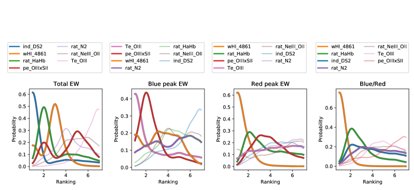
Figure 19: Variable importances for the equivalent width predictions. For details see caption of Figure 18.

The resulting luminosity predictions are shown in Figure 16 and the EW predictions in Figure 17. Colored points indicate the training part of the sample and black crosses show the testing sample. We use a 20 % test train split for training the models in this case. The errorbars are estimated by simple Monte Carlo simulation, where we resample all the predictors based on their error estimates and refit the model 2000 times.

Attending first to panel a of Figure 16 the models performs well with the a coefficient of determination (R²) of 0.8 meaning that it explains $\sim 80$% of the variance in the data. The performance of the model predicting the red peak (panel c) is very similar which is expected since the red peak represents a majority of the Ly$\alpha$ line flux. On the other hand the model predicting the blue peak performs worse, explaining around 50% of the variance—most likely due to the lower signal to noise in the blue peak compared to the red. The last panel (d) shows the model for the blue over red ratio. It is immediately apparent that the performance of this model is degraded compared to the others with $R^{2}$ around 0.2. This appears surprising given the decent performance of the red and blue separate models. One contributing factor is most likely that the dynamic range of the luminosities is significantly larger, which means that it is relatively easy to get the correct order of magnitude of the prediction, but when that large scale variation is removed, such as in a ratio, only the smaller scale variation remains which is harder to predict.

Figure 17 shows the results of our predictions of the Ly$\alpha$ EWs. The $R^{2}$ scores are lower for predicting the EW than the luminosity, which is expected because absolute values (e.g. luminosity) no longer enter when predicting the ratio of two quantities. However, models can still predict more than 50% of the variance. In this case we do not see a marked difference in performance between the total, blue and red models but the blue/red ratio model remains significantly worse.

We use a train-test-split to quantify the performance of the models when applied to galaxies that were not included in the fitting. The $R^{2}$ scores for the test samples are noted in the corresponding panels Figures 16 and 17. We note that they are in general, as expected, lower than the $R^{2}_{\mathrm{train}}$ scores, in some cases considerably so. This is an indication that the full models may be somewhat overfitting the data, however it is difficult to use the specific $R^{2}_{\mathrm{test}}$ score to evaluate to what degree, since the score is quite sensitive to the exact selection of train and test samples.

In order to reduce overfitting we need to reduce the number of included variables in the model. We can evaluate which variables to include and the effect on both train and test performance using variable selection, in this case forward selection. The method is quite simple. First we fit a 1-variable model using all variables individually and check, using the $R^{2}$ score, which is the best performing. This variable is selected as the most important. Then we fit a 2-variable model using the one that was selected and each of the remaining individually, with the best performing selected as the second most important variable. This is repeated for the whole set of predictors to give a complete set of rankings. We do this for each iteration of the Monte Carlo simulation which gives us a distribution of rankings for each variable which we then smooth with a kernel density estimator with a kernel size of 0.5. The resulting probability density functions are shown in Figure 18 and Figure 19 for the luminosity and equivalent width models respectively. The curves are ordered by the mean ranking of the variable with lowest rank, i.e. most important, first.

Attending first to the first panel of the luminosity variable selection, some patterns appear from the what at first seems a noisy plot. The two most important variables are the [O iii]₅₀₀₇ and [Ne iii]₃₈₆₉ lines, both clearly peaking at first rank. Both of these lines trace the high ionization gas. The second spot is shared by the [O ii] and [S ii] sums, both tracing low ionization gas. The first two variables then clearly correspond to ionization state tracers, c.f. the O₃₂, Ne3O2 or [S ii]/[O iii] ratios. After these ionization tracers H$\beta$ has the highest weight. Since we are predicting a luminosity our interpretation of this is that H$\beta$ acts as a flux normalization quantity. Additionally its dust attenuation is, most likely, closer to that of Ly$\alpha$ than for example H$\alpha$, due to the bluer wavelength.

The same patterns of importance are also seen in the predictions for the blue and red peak, with the only major difference being a reduced importance of H$\beta$. The biggest difference is notable in the prediction of the blue over red ratio. For this prediction lower ionization lines together with H$\alpha$ instead dominate. It is important not to over-interpret this since the prediction can in this case only explain about 30% of the variance in the sample.

Looking now to the equivalent width result, we find that there is more variance in the rankings across the different models. This is most likely due to the poorer performance of the models overall, but nevertheless some trends are clear. For instance the H$\beta$ equivalent width maintains a high degree of importance in all relations—in particular the red peak and blue over ratio models. This is in line with our expectations since a high H$\beta$ EW should correlate with a high production of Ly$\alpha$ photons as well as the evolutionary stage of the stars, and therefore potentially the Ly$\alpha$ EW. The H$\alpha$/H$\beta$ ratio, which encodes the dust extinction of the system, is also consistently ranked well. Again this is expected since dust is the primary destruction mechanism of Ly$\alpha$, however, what is less expected is that this variable seems to hold very little importance for the equivalent width of the blue peak. In fact the blue peak models seem dominated by thermodynamic variables, such as the temperature and pressure. While these variables describe the state of the gas and as such should impact Ly$\alpha$ transfer, we have found them to be only weakly correlated with Ly$\alpha$ properties throughout this work which makes this result surprising. Further, more complete multi-parametric analysis of these trends will be the topic of a forthcoming dedicated paper.

9 Summary, Conclusions and Outlook

In this paper we have performed an extensive and complete analysis of the medium resolution ultraviolet spectral data of local starburst galaxies, obtained with the Cosmic Origin Spectrograph on the Hubble Space Telescope. We have modeled the stellar continuum using population synthesis models to obtain many properties of the stellar population, including mass, metallicity, age, and inferred secondary quantities of ionizing photon production rates and mechanical energy returns. We have also measured the properties of over 40 optical emission lines in aperture-matched spectra, and measured quantities related to metal abundance, dust reddening, ionization state, and thermodynamic variables.

We show this full sample lies along standard loci in diagnostic diagrams, such as excitation and metallicity sequences (the ‘BPT diagrams’), the mass metallicity relation, and SFR-stellar mass diagram (the ‘star-forming main sequence’). There is a strong correlation between stellar metallicity and abundance estimates from the nebular gas, and also between starburst age and the equivalent width of H$\beta$ – in concert these show that our modeling is able to break the well-known age-metallicity degeneracy, and the quantities we refer to as ‘age’ meaningfully represent the evolutionary stage of the starburst episode. We conclude that our inferred stellar parameters are accurate.

In the UV spectra we have measured a large number of photometric and kinematic properties of the spectrally resolved Ly$\alpha$ emission line; we then use the properties derived from the nebular lines and stellar modeling to investigate how the Ly$\alpha$ output and spectral profile depend on physical conditions and how they may be predicted from other data. We back up some of these findings using estimates of the cool gas covering and kinematics, which are also derived from the UV spectra.

Our main conclusions are:

• Total Ly$\alpha$ output is strongest among young galaxies, when the most massive stars remain on the main sequence. Evidence for this is mainly provided by modeled age, and the equivalent width of Balmer lines. This is natural since a young stellar population is necessary to produce the maximum Ly$\alpha$ emission.

• Stellar age cannot uniquely explain the Ly$\alpha$ output. Ly$\alpha$ EW correlates most strongly with ionization parameter, as inferred from ratios of strong forbidden lines [O iii]/[O ii] and [Ne iii]/[O ii], and higher nebular EWs are also found among more highly ionized ISM conditions.

• The effects of age and ionization conditions do not only influence the Ly$\alpha$ production. Relations of equivalent amplitude and higher significance are found when contrasting these quantities with the Ly$\alpha$ escape fraction, which traces only the output and transfer of Ly$\alpha$ photons. These properties have a significant impact on the large scale ISM.

• Correlations with dust content are significant, but are insufficient to explain the Ly$\alpha$ output. Since ionization parameter is the strongest correlating variable, we expect that the main factor in influencing Ly$\alpha$ emission at early times, and therefore the observed EW, is the ionization condition. The H i column density is reduced by the extreme ionizing conditions and the Ly$\alpha$ transfer is eased.

• This conclusion is further supported by the resolved Ly$\alpha$ line profile, which shows more blueshifted emission at early times and with higher ionization parameters. Most of the relations described above hold for the blue and red components of the line, but relations for the blueshifted part alone exhibit a larger dynamic range.

• By stacking the ultraviolet continuum spectra and examining the low ionization absorption lines, we see that all these phenomena are directly associated with the column of absorbing gas. This decreases towards younger ages and higher ionization parameters, reduces the Ly$\alpha$ scattering, and leads to higher escape fractions. Moreover, the column of gas at zero velocity is lowest in the galaxies with highest contributions of blueshifted Ly$\alpha$, indicating that the removal of this gas by photoionization at early times is responsible for the blueshifted emission.

• Simple multi-parametric analysis can predict up to 80% of the variance in the Ly$\alpha$ luminosity, performing equally well for the total and red peak. Similar models can predict approximately 50% of the variance in the EWs.

• We use variable selection methods to quantify which variables carry the most weight in the relations. We find that the luminosity relations appear dominated by ionization tracers such as [O iii] and [Ne iii] together with low ionization lines like [O ii]. This is in line with the correlation analysis presented earlier in this work. We also find that H$\beta$ provides a better absolute value calibration than H$\alpha$ most likely due to the effect of the bluer wavelength on the dust attenuation. In this multi-parametric experiment we are unable to predict the $L_{\mathrm{B/R}}$ ratio.

• The variable selection results for the EW relations is somewhat less clear cut but does seem to give preference to dust tracers, in this case H$\alpha$/H$\beta$ and to the H$\beta$ EW. Improving these multi-parametric estimates will be the subject of future work.

• We have no uniform estimates of the inclination nor morphology of our galaxies, and neither can we estimate the influence of viewing angle on the Ly$\alpha$ escape. These effects would cause our observations to miss Ly$\alpha$ in some cases, and must certainly contribute scatter to some of the relations, hiding some of the weaker trends.

Data Availability

All data are available in the Barbara A. Mikulski Archive for Space Telescopes (MAST) at https://archive.stsci.edu/hst/search.php

Appendix A Galaxy Coordinates and Redshifts

Table 1: Galaxy names and properties

Name	Right Ascension	Declination	Redshift	$M_{\mathrm{UV}}$	SFR(H$\alpha$)	$E_{B-V}$	12+log(O/H)	log($L_{\mathrm{Ly}\alpha}$)
	[∘] J2000	[∘] J2000			[M⊙ yr-1]	[mag]		erg s-1
SDSSJ0055-0021	$13.86446$	$-0.36349$	$0.16743$	$-20.33$	$35.01$	$0.227$	$8.19$	$41.45$
SDSSJ0150+1308	$27.61838$	$13.14956$	$0.14674$	$-20.54$	$18.61$	$0.188$	$8.30$	$41.37$
SDSSJ0213+1259	$33.45221$	$12.99761$	$0.21897$	$-20.36$	$34.47$	$1.024$	$8.49$	$41.70$
SDSSJ0808+3948	$122.18450$	$39.81459$	$0.09125$	$-19.97$	$5.91$	$0.326$	$8.53$	$42.01$
SDSSJ0921+4509	$140.49746$	$45.15344$	$0.23500$	$-21.02$	$29.59$	$0.416$	$8.48$	$41.49$
SDSSJ0926+4427	$141.50183$	$44.46015$	$0.18068$	$-20.84$	$21.79$	$0.096$	$8.02$	$42.78$
SDSSJ0938+5428	$144.55621$	$54.47364$	$0.10207$	$-20.43$	$21.47$	$0.174$	$8.16$	$41.34$
SDSSJ2103-0728	$315.99475$	$-7.46736$	$0.13688$	$-20.32$	$16.69$	$0.108$	$8.49$	$42.21$
SDSSJ0021+0052	$5.25429$	$0.88003$	$0.09835$	$-20.90$	$20.11$	$0.044$	$8.12$	$42.59$
SDSSJ1025+3622	$156.45158$	$36.38289$	$0.12650$	$-20.20$	$16.07$	$0.136$	$8.09$	$42.31$
SDSSJ1112+5503	$168.18354$	$55.06306$	$0.13164$	$-99.00$	$27.33$	$0.208$	$8.37$	$41.87$
SDSSJ1144+4012	$176.09283$	$40.20589$	$0.12694$	$-20.46$	$11.52$	$0.322$	$8.30$	$40.73$
SDSSJ1414+0540	$213.72554$	$5.67989$	$0.08186$	$-20.26$	$10.02$	$0.286$	$8.21$	$40.55$
SDSSJ1416+1223	$214.05363$	$12.39456$	$0.12315$	$-20.60$	$24.02$	$0.260$	$8.34$	$41.18$
SDSSJ1428+1653	$217.23504$	$16.89426$	$0.18167$	$-21.29$	$27.71$	$0.169$	$8.24$	$42.46$
SDSSJ1429+0643	$217.44583$	$6.72637$	$0.17353$	$-20.92$	$42.88$	$0.048$	$8.08$	$42.73$
SDSSJ1521+0759	$230.42258$	$7.98937$	$0.09426$	$-20.23$	$8.53$	$0.187$	$8.20$	$41.64$
SDSSJ1612+0817	$243.18967$	$8.28361$	$0.14914$	$-20.84$	$38.59$	$0.303$	$8.35$	$42.31$
GP0303-0759	$45.83921$	$-7.98978$	$0.16485$	$-20.56$	$13.48$	$-0.041$	$8.02$	$41.94$
GP0911+1831	$137.80558$	$18.51894$	$0.26220$	$-20.99$	$32.52$	$0.159$	$8.20$	$42.81$
GP1054+5238	$163.37833$	$52.63136$	$0.25263$	$-21.31$	$38.74$	$0.078$	$8.12$	$42.54$
GP1133+6514	$173.26583$	$65.22817$	$0.24140$	$-20.79$	$8.72$	$0.022$	$8.06$	$42.58$
GP1137+3524	$174.34225$	$35.40742$	$0.19437$	$-20.86$	$27.82$	$0.047$	$8.10$	$42.62$
GP1219+1526	$184.76658$	$15.43569$	$0.19563$	$-20.78$	$19.65$	$-0.029$	$8.00$	$43.19$
GP1244+0216	$191.09737$	$2.26122$	$0.23943$	$-20.66$	$43.90$	$0.066$	$8.07$	$42.56$
GP1249+1234	$192.14429$	$12.56747$	$0.26339$	$-20.91$	$24.78$	$0.080$	$8.05$	$43.07$
GP1424+4217	$216.02383$	$42.27953$	$0.18477$	$-20.79$	$30.47$	$0.064$	$8.05$	$42.94$
J0925+1403	$141.38487$	$14.05363$	$0.30123$	$-20.47$	$26.92$	$0.075$	$8.01$	$42.83$
J1152+3400	$178.02033$	$34.01386$	$0.34193$	$-20.77$	$21.29$	$0.001$	$8.02$	$43.00$
J1333+6246	$203.26650$	$62.76772$	$0.31812$	$-20.52$	$-99.00$	$-99.000$	$8.09$	$42.75$
J1442-0209	$220.63079$	$-2.16445$	$0.29368$	$-21.11$	$29.37$	$0.104$	$7.93$	$43.16$
J1503+3644	$225.92846$	$36.74743$	$0.35569$	$-20.43$	$23.11$	$0.068$	$8.04$	$42.86$
J0901+2119	$135.44004$	$21.32438$	$0.29931$	$-19.06$	$15.92$	$0.072$	$7.99$	$42.48$
J1011+1947	$152.90950$	$19.78915$	$0.33217$	$-19.33$	$33.73$	$0.302$	$7.92$	$42.64$
J1154+2443	$178.70354$	$24.72584$	$0.36899$	$-19.50$	$12.74$	$0.135$	$7.92$	$42.87$
J1243+4646	$190.75262$	$46.78067$	$0.43171$	$-20.67$	$23.77$	$0.098$	$7.70$	$43.08$
J1248+4259	$192.04367$	$42.99822$	$0.36302$	$-99.00$	$25.27$	$0.025$	$7.93$	$42.79$
J1256+4509	$194.18396$	$45.15472$	$0.35320$	$-19.85$	$11.24$	$0.076$	$7.93$	$42.54$
J0159+0751	$29.96979$	$7.86356$	$0.06106$	$-16.58$	$1.99$	$0.258$	$7.79$	$41.59$
J1205+4551	$181.26479$	$45.86415$	$0.06539$	$-16.41$	$2.91$	$0.131$	$8.01$	$41.65$
J1242+4851	$190.61025$	$48.86602$	$0.06216$	$-15.81$	$0.70$	$0.009$	$7.69$	$41.44$
SDSSJ0815+2156	$123.96667$	$21.93990$	$0.14095$	$-19.25$	$7.04$	$0.040$	$7.96$	$42.34$
J0240-0828	$40.21746$	$-8.47428$	$0.08224$	$-18.20$	$8.63$	$0.067$	$7.99$	$42.32$
J0851+5840	$132.81521$	$58.68194$	$0.09190$	$-18.35$	$9.21$	$0.108$	$7.97$	$41.64$
J1200+2719	$180.06867$	$27.33306$	$0.08188$	$-18.83$	$8.01$	$0.123$	$7.95$	$42.43$
J1226+0415	$186.54954$	$4.26002$	$0.09422$	$-18.06$	$10.24$	$0.168$	$8.00$	$42.02$
J1311-0038	$197.88033$	$-0.64566$	$0.08106$	$-18.08$	$5.25$	$0.184$	$8.03$	$42.03$
GP0822+2241	$125.69859$	$22.69558$	$0.21622$	$-20.12$	$52.36$	$0.198$	$8.06$	$42.35$
GP0917+3152	$139.26052$	$31.87238$	$0.30038$	$-20.96$	$25.55$	$0.176$	$8.22$	$42.59$
GP1009+2916	$152.32914$	$29.27264$	$0.22192$	$-19.75$	$7.53$	$0.069$	$8.01$	$42.34$
GP1122+6154	$170.58222$	$61.91263$	$0.20456$	$-19.24$	$9.17$	$0.150$	$8.06$	$42.26$
GP1440+4619	$220.04142$	$46.32693$	$0.30078$	$-21.43$	$47.94$	$0.137$	$8.13$	$42.81$
GP1454+4528	$223.64825$	$45.48231$	$0.26852$	$-20.31$	$27.91$	$0.181$	$8.17$	$42.27$
GP1514+3852	$228.53598$	$38.86871$	$0.33263$	$-20.68$	$9.38$	$-0.275$	$8.14$	$42.76$
GP1559+0841	$239.85824$	$8.68865$	$0.29719$	$-19.80$	$-99.00$	$-99.000$	$8.18$	$42.57$
GP2237+1336	$339.39608$	$13.61306$	$0.29350$	$-21.15$	$41.17$	$0.136$	$8.10$	$42.29$
GALEX1417+5228	$214.43094$	$52.46828$	$0.20813$	$-18.28$	$1.77$	$-0.083$	$7.68$	$42.06$
J0232-0426	$38.06704$	$-4.44076$	$0.45237$	$-99.00$	$9.52$	$0.101$	$7.96$	$42.58$
J0919+4906	$139.98241$	$49.10243$	$0.40515$	$-19.28$	$6.24$	$0.041$	$7.99$	$42.75$
J1046+5827	$161.50825$	$58.46582$	$0.39675$	$-20.40$	$8.93$	$-0.061$	$7.93$	$42.59$
J1121+3806	$170.32591$	$38.11189$	$0.31787$	$-99.00$	$4.80$	$-0.017$	$7.96$	$42.47$
J1127+4610	$171.83750$	$46.17847$	$0.32221$	$-99.00$	$4.45$	$-0.139$	$7.88$	$42.15$
J1233+4959	$188.37825$	$49.99707$	$0.42199$	$-99.00$	$10.12$	$-0.050$	$8.03$	$42.72$
J1349+5631	$207.47958$	$56.51969$	$0.36361$	$-99.00$	$6.57$	$0.157$	$8.03$	$42.32$
J1355+1457	$208.97275$	$14.95041$	$0.36513$	$-99.00$	$11.92$	$0.060$	$7.92$	$42.56$
J1455+6107	$223.99820$	$61.12214$	$0.36786$	$-20.05$	$7.17$	$-0.022$	$7.99$	$42.57$
J010534+234960	$16.39057$	$23.83325$	$0.33807$	$-19.71$	$22.32$	$0.121$	$8.09$	$42.69$
J015208-043117	$28.03331$	$-4.52145$	$0.38359$	$-20.23$	$24.67$	$0.168$	$8.15$	$42.79$
J020819-040136	$32.07877$	$-4.02679$	$0.38445$	$-20.56$	$16.32$	$-0.130$	$8.02$	$42.92$
J110359+483456	$165.99582$	$48.58219$	$0.41795$	$-20.25$	$24.49$	$0.177$	$8.07$	$42.64$
J110506+594741	$166.27636$	$59.79484$	$0.40540$	$-19.72$	$17.02$	$0.155$	$8.06$	$42.80$
J121948+481411	$184.94943$	$48.23625$	$0.42022$	$-20.42$	$13.69$	$0.055$	$8.10$	$42.63$
J124619+444902	$191.58118$	$44.81730$	$0.32217$	$-20.75$	$40.72$	$0.150$	$8.07$	$42.88$
J142535+524902	$216.39628$	$52.81728$	$0.38695$	$-19.74$	$17.46$	$0.156$	$7.97$	$42.49$
Names are according to MAST archive labeling.
$M_{\mathrm{UV}}$ is corrected for Milky Way extinction.
SFR(H$\alpha$) is corrected for internal attenuation and uses the Kennicutt & Evans (2012) calibration
Oxygen abundance is derived from the O3N2 index using Marino et al. (2013).
$L_{\mathrm{Ly}\alpha}$ is derived from the Lyman alpha Spectral Database (LASD Runnholm et al., 2021).

References

- Adams (1972) Adams T. F., 1972, ApJ, 174, 439
- Ahumada et al. (2020) Ahumada R., et al., 2020, ApJS, 249, 3
- Asplund et al. (2009) Asplund M., Grevesse N., Sauval A. J., Scott P., 2009, ARA&A, 47, 481
- Atek et al. (2009) Atek H., Kunth D., Schaerer D., Hayes M., Deharveng J. M., Östlin G., Mas-Hesse J. M., 2009, A&A, 506, L1
- Atek et al. (2014) Atek H., Kunth D., Schaerer D., Mas-Hesse J. M., Hayes M., Östlin G., Kneib J.-P., 2014, A&A, 561, A89
- Baldwin et al. (1981) Baldwin J. A., Phillips M. M., Terlevich R., 1981, PASP, 93, 5
- Berg et al. (2012) Berg D. A., et al., 2012, ApJ, 754, 98
- Bergvall et al. (2013) Bergvall N., Leitet E., Zackrisson E., Marquart T., 2013, A&A, 554, A38
- Calzetti et al. (2000) Calzetti D., Armus L., Bohlin R. C., Kinney A. L., Koornneef J., Storchi-Bergmann T., 2000, ApJ, 533, 682
- Cardelli et al. (1989) Cardelli J. A., Clayton G. C., Mathis J. S., 1989, ApJ, 345, 245
- Carr et al. (2018) Carr C., Scarlata C., Panagia N., Henry A., 2018, ApJ, 860, 143
- Carr et al. (2021) Carr C., Scarlata C., Henry A., Panagia N., 2021, ApJ, 906, 104
- Charlot & Fall (2000) Charlot S., Fall S. M., 2000, ApJ, 539, 718
- Childs & Stanway (2018) Childs H. J. T., Stanway E. R., 2018, MNRAS, 480, 1938
- Chisholm et al. (2017) Chisholm J., Tremonti C. A., Leitherer C., Chen Y., 2017, MNRAS, 469, 4831
- Chisholm et al. (2019) Chisholm J., Rigby J. R., Bayliss M., Berg D. A., Dahle H., Gladders M., Sharon K., 2019, ApJ, 882, 182
- Claeyssens et al. (2019) Claeyssens A., et al., 2019, MNRAS, 489, 5022
- Curti et al. (2020) Curti M., Mannucci F., Cresci G., Maiolino R., 2020, MNRAS, 491, 944
- Draine (2011) Draine B. T., 2011, Physics of the Interstellar and Intergalactic Medium
- Drake et al. (2017) Drake A. B., et al., 2017, A&A, 608, A6
- Erb et al. (2006) Erb D. K., Shapley A. E., Pettini M., Steidel C. C., Reddy N. A., Adelberger K. L., 2006, ApJ, 644, 813
- Flury et al. (2022) Flury S. R., et al., 2022, arXiv e-prints, p. arXiv:2203.15649
- France et al. (2010) France K., Nell N., Green J. C., Leitherer C., 2010, ApJ, 722, L80
- Gazagnes et al. (2018) Gazagnes S., Chisholm J., Schaerer D., Verhamme A., Rigby J. R., Bayliss M., 2018, A&A, 616, A29
- Gazagnes et al. (2020) Gazagnes S., Chisholm J., Schaerer D., Verhamme A., Izotov Y., 2020, A&A, 639, A85
- Gronke (2017) Gronke M., 2017, A&A, 608, A139
- Hayes (2015) Hayes M., 2015, PASA, 32, 27
- Hayes (2023) Hayes M. J., 2023, MNRAS, 519, L26
- Hayes et al. (2005) Hayes M., Östlin G., Mas-Hesse J. M., Kunth D., Leitherer C., Petrosian A., 2005, A&A, 438, 71
- Hayes et al. (2010) Hayes M., et al., 2010, Nature, 464, 562
- Hayes et al. (2014) Hayes M., et al., 2014, ApJ, 782, 6
- Hayes et al. (2021) Hayes M. J., Runnholm A., Gronke M., Scarlata C., 2021, ApJ, 908, 36
- Heckman & Borthakur (2016) Heckman T. M., Borthakur S., 2016, ApJ, 822, 9
- Heckman et al. (2015) Heckman T. M., Alexandroff R. M., Borthakur S., Overzier R., Leitherer C., 2015, ApJ, 809, 147
- Henry et al. (2015) Henry A., Scarlata C., Martin C. L., Erb D., 2015, ApJ, 809, 19
- Herenz et al. (2017) Herenz E. C., et al., 2017, A&A, 606, A12
- Herenz et al. (2019) Herenz E. C., et al., 2019, A&A, 621, A107
- Herenz et al. (2020) Herenz E. C., Hayes M., Scarlata C., 2020, A&A, 642, A55
- Hoag et al. (2019) Hoag A., et al., 2019, MNRAS, 488, 706
- Izotov et al. (2017) Izotov Y. I., Thuan T. X., Guseva N. G., 2017, MNRAS, 471, 548
- Izotov et al. (2020) Izotov Y. I., Schaerer D., Worseck G., Verhamme A., Guseva N. G., Thuan T. X., Orlitová I., Fricke K. J., 2020, MNRAS, 491, 468
- Izotov et al. (2021) Izotov Y. I., Worseck G., Schaerer D., Guseva N. G., Chisholm J., Thuan T. X., Fricke K. J., Verhamme A., 2021, MNRAS, 503, 1734
- Jaskot & Oey (2014) Jaskot A. E., Oey M. S., 2014, ApJ, 791, L19
- Jaskot et al. (2017) Jaskot A. E., Oey M. S., Scarlata C., Dowd T., 2017, ApJ, 851, L9
- Jaskot et al. (2019) Jaskot A. E., Dowd T., Oey M. S., Scarlata C., McKinney J., 2019, ApJ, 885, 96
- Jiang et al. (2013) Jiang L., et al., 2013, ApJ, 773, 153
- Kakiichi & Gronke (2021) Kakiichi K., Gronke M., 2021, ApJ, 908, 30
- Kashikawa et al. (2006) Kashikawa N., et al., 2006, ApJ, 648, 7
- Kauffmann et al. (2003) Kauffmann G., et al., 2003, MNRAS, 346, 1055
- Kehrig et al. (2018) Kehrig C., Vílchez J. M., Guerrero M. A., Iglesias-Páramo J., Hunt L. K., Duarte-Puertas S., Ramos-Larios G., 2018, MNRAS, 480, 1081
- Kennicutt & Evans (2012) Kennicutt R. C., Evans N. J., 2012, ARA&A, 50, 531
- Kewley & Dopita (2002) Kewley L. J., Dopita M. A., 2002, ApJS, 142, 35
- Kewley et al. (2001) Kewley L. J., Dopita M. A., Sutherland R. S., Heisler C. A., Trevena J., 2001, ApJ, 556, 121
- Kreckel et al. (2013) Kreckel K., et al., 2013, ApJ, 771, 62
- Kunth et al. (1998) Kunth D., Mas-Hesse J. M., Terlevich E., Terlevich R., Lequeux J., Fall S. M., 1998, A&A, 334, 11
- Le Reste et al. (2022) Le Reste A., et al., 2022, arXiv e-prints, p. arXiv:2206.06374
- Leitherer et al. (1999) Leitherer C., et al., 1999, ApJS, 123, 3
- Leitherer et al. (2014) Leitherer C., Ekström S., Meynet G., Schaerer D., Agienko K. B., Levesque E. M., 2014, ApJS, 212, 14
- Levesque & Richardson (2014) Levesque E. M., Richardson M. L. A., 2014, ApJ, 780, 100
- Lidman et al. (2012) Lidman C., Hayes M., Jones D. H., Schaerer D., Westra E., Tapken C., Meisenheimer K., Verhamme A., 2012, MNRAS, 420, 1946
- Luridiana et al. (2015) Luridiana V., Morisset C., Shaw R. A., 2015, A&A, 573, A42
- Maiolino et al. (2008) Maiolino R., et al., 2008, A&A, 488, 463
- Marchi et al. (2019) Marchi F., et al., 2019, A&A, 631, A19
- Marino et al. (2013) Marino R. A., et al., 2013, A&A, 559, A114
- Marques-Chaves et al. (2022) Marques-Chaves R., et al., 2022, A&A, 663, L1
- Mas-Hesse et al. (2003) Mas-Hesse J. M., Kunth D., Tenorio-Tagle G., Leitherer C., Terlevich R. J., Terlevich E., 2003, ApJ, 598, 858
- Mason et al. (2018) Mason C. A., et al., 2018, ApJ, 857, L11
- Matthee et al. (2021) Matthee J., et al., 2021, MNRAS, 505, 1382
- Matthee et al. (2022) Matthee J., et al., 2022, MNRAS, 512, 5960
- Meurer et al. (1995) Meurer G. R., Heckman T. M., Leitherer C., Kinney A., Robert C., Garnett D. R., 1995, AJ, 110, 2665
- Naidu et al. (2022) Naidu R. P., et al., 2022, MNRAS, 510, 4582
- Nakajima & Ouchi (2014) Nakajima K., Ouchi M., 2014, MNRAS, 442, 900
- Natta & Panagia (1984) Natta A., Panagia N., 1984, ApJ, 287, 228
- Neufeld (1990) Neufeld D. A., 1990, ApJ, 350, 216
- Olivier et al. (2021) Olivier G. M., Berg D. A., Chisholm J., Erb D. K., Pogge R. W., Skillman E. D., 2021, arXiv e-prints, p. arXiv:2109.06725
- Osterbrock (1962) Osterbrock D. E., 1962, ApJ, 135, 195
- Ouchi et al. (2020) Ouchi M., Ono Y., Shibuya T., 2020, ARA&A, 58, 617
- Pettini & Pagel (2004) Pettini M., Pagel B. E. J., 2004, MNRAS, 348, L59
- Reddy et al. (2015) Reddy N. A., et al., 2015, ApJ, 806, 259
- Remolina-Gutiérrez & Forero-Romero (2019) Remolina-Gutiérrez M. C., Forero-Romero J. E., 2019, MNRAS, 482, 4553
- Rhoads et al. (2003) Rhoads J. E., et al., 2003, AJ, 125, 1006
- Rivera-Thorsen et al. (2015) Rivera-Thorsen T. E., et al., 2015, ApJ, 805, 14
- Runnholm et al. (2020) Runnholm A., Hayes M., Melinder J., Rivera-Thorsen E., Östlin G., Cannon J., Kunth D., 2020, ApJ, 892, 48
- Runnholm et al. (2021) Runnholm A., Gronke M., Hayes M., 2021, PASP, 133, 034507
- Saldana-Lopez et al. (2022) Saldana-Lopez A., et al., 2022, arXiv e-prints, p. arXiv:2201.11800
- Santini et al. (2017) Santini P., et al., 2017, ApJ, 847, 76
- Scarlata & Panagia (2015) Scarlata C., Panagia N., 2015, ApJ, 801, 43
- Scarlata et al. (2009) Scarlata C., et al., 2009, ApJ, 704, L98
- Schaerer & Verhamme (2008) Schaerer D., Verhamme A., 2008, A&A, 480, 369
- Schlafly & Finkbeiner (2011) Schlafly E. F., Finkbeiner D. P., 2011, ApJ, 737, 103
- Senchyna et al. (2020) Senchyna P., Stark D. P., Mirocha J., Reines A. E., Charlot S., Jones T., Mulchaey J. S., 2020, MNRAS, 494, 941
- Senchyna et al. (2022) Senchyna P., et al., 2022, ApJ, 930, 105
- Shapley et al. (2003) Shapley A. E., Steidel C. C., Pettini M., Adelberger K. L., 2003, ApJ, 588, 65
- Shimasaku et al. (2006) Shimasaku K., et al., 2006, PASJ, 58, 313
- Sirressi et al. (2022) Sirressi M., et al., 2022, MNRAS, 510, 4819
- Stark et al. (2010) Stark D. P., Ellis R. S., Chiu K., Ouchi M., Bunker A., 2010, MNRAS, 408, 1628
- Stark et al. (2017) Stark D. P., et al., 2017, MNRAS, 464, 469
- Stasińska (2006) Stasińska G., 2006, A&A, 454, L127
- Steidel et al. (2016) Steidel C. C., Strom A. L., Pettini M., Rudie G. C., Reddy N. A., Trainor R. F., 2016, ApJ, 826, 159
- Tremonti et al. (2004) Tremonti C. A., et al., 2004, ApJ, 613, 898
- U et al. (2015) U V., et al., 2015, ApJ, 815, 57
- Urrutia et al. (2019) Urrutia T., et al., 2019, A&A, 624, A141
- Vanzella et al. (2010) Vanzella E., et al., 2010, A&A, 513, A20
- Vázquez & Leitherer (2005) Vázquez G. A., Leitherer C., 2005, ApJ, 621, 695
- Verhamme et al. (2006) Verhamme A., Schaerer D., Maselli A., 2006, A&A, 460, 397
- Verhamme et al. (2008) Verhamme A., Schaerer D., Atek H., Tapken C., 2008, A&A, 491, 89
- Verhamme et al. (2015) Verhamme A., Orlitová I., Schaerer D., Hayes M., 2015, A&A, 578, A7
- Verhamme et al. (2017) Verhamme A., Orlitová I., Schaerer D., Izotov Y., Worseck G., Thuan T. X., Guseva N., 2017, A&A, 597, A13
- Wang et al. (2019) Wang B., Heckman T. M., Leitherer C., Alexandroff R., Borthakur S., Overzier R. A., 2019, ApJ, 885, 57
- Wang et al. (2021) Wang B., et al., 2021, ApJ, 916, 3
- Wofford et al. (2021) Wofford A., Vidal-García A., Feltre A., Chevallard J., Charlot S., Stark D. P., Herenz E. C., Hayes M., 2021, MNRAS, 500, 2908
- Xu et al. (2022) Xu X., et al., 2022, ApJ, 933, 202
- Yin et al. (2007) Yin S. Y., Liang Y. C., Hammer F., Brinchmann J., Zhang B., Deng L. C., Flores H., 2007, A&A, 462, 535