Anomalous diffusion, non-Gaussianity, and nonergodicity for subordinated fractional Brownian motion with a drift

Abstract

The stochastic motion of a particle with long-range correlated increments (the moving phase) which is intermittently interrupted by immobilizations (the traping phase) in a disordered medium is considered in the presence of an external drift. In particular, we consider trapping events whose times follow a scale-free distribution with diverging mean trapping time. We construct this process in terms of fractional Brownian motion (FBM) with constant forcing in which the trapping effect is introduced by the subordination technique, connecting "operational time" with observable "real time". We derive the statistical properties of this process such as non-Gaussianity and non-ergodicity, for both ensemble and single-trajectory (time) averages. We demonstrate nice agreement with extensive simulations for the probability density function, skewness, kurtosis, as well as ensemble and time-averaged mean squared displacements. We pay specific emphasis on the comparisons between the cases with and without drift.

I Introduction

Brownian motion (normal diffusion) is characterized by a mean squared displacement (MSD) of a tracer particle that is a linear function of time vankampen ; haenggirev ; spiecho ; levybrown . Moreover, the probability density function (PDF) of the displacements is Gaussian. The emergence of such normal diffusion rests on the following three conditions: (i) there exists a finite correlation time after which individual displacements become independent, (ii) the displacements are identically distributed, and (iii) the second moment of the displacements is finite. Anomalous diffusion, in contradistinction, which may appear whenever one of these conditions is violated, has been widely observed in systems ranging from soft and bio matter over condensed matter, up to financial markets or geophysical systems bouc ; magi13 ; sun ; bols ; soko ; metz00 ; metz14 . In anomalous diffusion the MSD follows the power-law form

$$\langle x^{2}(t)\rangle\sim K_{\alpha}t^{\alpha},$$ (1)

where the anomalous diffusion coefficient has physical dimension $[K_{\alpha}]=\mathrm{length}^{2}/\mathrm{time}^{\alpha}$. Depending on the value of the anomalous diffusion exponent we distinguish subdiffusion for $0<\alpha<1$ from superdiffusion for $\alpha>1$ bouc ; metz00 ; soko ; bark12 . Examples for subdiffusion include the motion of submicron tracers in the crowded environment of living biological cells golding ; weber ; lene or in polymer-crowded in vitro liquids szym ; lene1 , the motion of potassium channels resident in the plasma membranes of living cells bark12 ; pt1 . For superdiffusion we mention motor-driven transport of viruses seis , neuronal messenger ribonucleoprotein song , endogeneous cellular vesicels christine or magnetic endosomes robe10 .

As soon as one or more of the above three conditions for normal diffusion are violated, the resulting stochastic process is no longer universal in the sense that a given measured MSD (1) may result from different processes soko ; bark12 ; pt1 ; metz14 . The inference of such processes from data has received considerable attention, approaches including the construction of decision trees based on complementary statistical observables yazmine , dynamic scaling exponents philipp ; vilk1 , or p-variations marcin , as well as "objective" methods such as Bayesian analysis michael ; samu ; samu1 or machine learning yael ; gorka ; janusz ; janusz1 ; bo ; andi ; henrik , inter alia.

Here we consider the case when two specific, fundamental anomalous stochastic processes are combined in the presence of an external drift. These two processes are fractional Brownian motion (FBM) and the subdiffusive continuous time random walk (CTRW). Going back to Kolmogorov kolmo and Mandelbrot and van Ness mand , FBM is a non-Markovian process driven by zero-mean, stationary Gaussian noise with long-range correlations. FBM can describe both sub- and superdiffusion, depending on whether the noise is antipersistent or persistent (see below). Examples for subdiffusive FBM-type motion include tracer motion in complex liquids szym ; lene1 and in the cytoplasm of living cells lene ; weber , or lipid dynamics in bilayer membranes jeon . Superdiffusive FBM was found for the motion of higher animals vilk1 and of vacuoles in amoeboid cells and the amoeba cells themselves krap , and it is used as a model for densities of persistently growing brain fibers janu20 .

The continuous time random walk (CTRW) model introduced by Montroll and Weiss mont is a generalization of a random walk in which the particle waits for a random time $\tau$ between jumps. When the associated PDF of waiting times is scale free, $\psi(\tau)\simeq\tau^{-1-\alpha}$ with $0<\alpha<1$, such that the mean waiting time $\langle\tau\rangle$ diverges, subdiffusion of the form (1) emerges, where the anomalous diffusion exponent is given by the scaling exponent of the waiting time PDF. Examples for such CTRW subdiffusion include the motion of charge carriers in amorphous semiconductors scher ; neher , and (asymptotic) power-law forms for the waiting times $\tau$ were identified, i.a., for the motion of potassium channels in live cell membranes weig , in glass-forming liquids rubn , for drug molecules diffusing in between two silica slabs amanda , and for tracer transport in geological formations berk .

There exist a growing number of examples in which analysis of the recorded dynamics demonstrates the conspirative action of more than a single anomalous diffusion process. In particular, we here mention systems in which CTRW and FBM simultaneously. These include the motion of insulin granules in living MIN6 insulisoma cells tabei , of nicotinic acetylcholine membrane receptors mosqueira , nanosized tracer objects in the cytoplasm etoc , drug molecules confined by silica slabs amanda , and of voltage-gated sodium channels on the surface of hippocampal neurons fox .

The combined stochastic process of long-range correlated FBM and scale-free waiting time effects was recently studied in terms of a subordination concept in fox . We here go one step beyond and study this type of stochastic motion in the presence of a constant external drift. To this end we start our description with an FBM process, which is then subordinated to a stable subordinator appl ; boch ; fell ; chec21 ; meer13 ; meer04 ; magd ; wang22 . Historically, the notion of subordination was introduced by Bochner boch and applied by Feller fell . The dynamics of the process of interest here thus involves three elements, namely, long-range correlations, scale-free waiting times, and an external drift. We here investigate analyitcally and numerically the transport properties of this process.

The paper is organized as follows. In Sec. II, the Langevin equation for subordinated FBM in the presence of a drift is introduced. Sec. III provides the PDF and shows its non-Gaussianity. We also obtain the ensemble-averaged MSD. In Sec. IV the time-averaged MSD (TAMSD) is derived, discussing the weakly non-ergodic statistic along with the amplitude scatter of the TAMSD. The results are discussed in Sec. V. For the convenience of the reader the results for subordinated FBM without drift are briefly summarized in App. A.

II Subordinated fractional Brownian motion with drift

Subordinated FBM with drift, $x(t)\equiv x(s(t))$ combines both long trapping times and long-range correlations with a drift. It satisfies the coupled stochastic equations

$$\frac{dx(s)}{ds} = v+\sqrt{2D}\zeta_{H}(s),$$

$$\frac{dt(s)}{ds} = \varepsilon(s),$$ (2)

see the discussions in fogedby ; magd . Here $x(s)$ is the particle trajectory as function of "operational time" $s$, and $v$ is the constant external drift. Without loss of generality we set $D=0.5$. Moreover, $\zeta_{H}(s)$ represents fractional Gaussian noise with correlation function $\langle\zeta_{H}(t_{1})\zeta_{H}(t_{2})\rangle\sim H(2H-1)|t_{1}-t_{2}|^{2H-2}$, for $t_{1}\neq t_{2}$ mand . Here, $H$ with $0<H<1$ is the Hurst exponent. For free FBM, this effects the MSD (1) with $\alpha=2H$. The second equation then translates the operational time $s$ into the "real" process time $t$, where $\varepsilon(s)$ represents one-sided Lévy stable noise gawr ; pens10 , which is the formal derivative of the Lévy stable subordinator $t(s)$ with stability index $0<\alpha<1$. The Lévy stable subordinator is a non-decreasing Lévy process with stationary and independent increments. The one-sided Lévy stable distribution saa ; pens16 ; datt is defined in terms of its Laplace transform via $\hat{L}_{\alpha}(k)=\exp(-k^{\alpha})$, which is strictly increasing. The inverse subordinator $s(t)$ is defined as $s(t)=\inf\{s>0:t(s)>t\}$, where $s(t)$ is called the hitting time or first-passage time process meer13 , which can be considered as the limit process of the continuous time random walk with a heavy tailed waiting time PDF. It tends to infinity when $t\to\infty$. We note that the distribution of $s(t)$ is also called the Mittag-Leffler distribution based on the relationship between the moments and the Mittag-Leffler function saa . The subordinator $s(t)$ is responsible for the subdiffusive behavior with long rests of the particle, while the parent process $x(s)$ introduces the correlated FBM with drift.

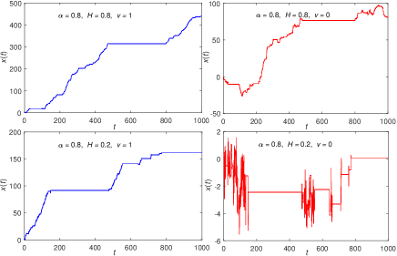
Figure 1: Sample trajectories of subordinated FBM $x(t)$ with drift $v=1$ and without drift ($v=0$) for different values of the Hurst exponent $H$ (see the legends in the panels) of the parental FBM and waiting time index $\alpha=0.8$. Note the different spans of the vertical axes. The elementary time step in the simulations was $dt=0.1$.

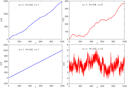
Figure S4: Sample trajectories of subordinated FBM with drift $v=1$ and without drift ($v=0$) for the cases $H=0.8$ and $H=0.2$ with $\alpha=1$.

Fig. 1 shows sample trajectories of subordinated FBM with drift $v=1$ and without drift ($v=0$) for two values of the Hurst index (persisent, i.e., positively correlated FBM, with $H=0.8$ and anti-persistent, negatively correlated FBM with $H=0.2$), and for $\alpha=0.8$. We use identical noise time series of the fractional Gaussian noise time series and the subordinator for each $H$ value. The cases for $\alpha=1$, i.e., without long waiting times, are shown in Fig. S4 in App. A. Even for the relatively large waiting time exponent $\alpha=0.8$ the effects of immobilization are clearly present.

III Probability density function, moments, and ensemble-averaged mean squared displacement

The PDF of the subordinated process is bark

$$P(x,t)=\int_{0}^{+\infty}P_{0}(x,s)h(s,t)ds,$$ (3)

where $P_{0}(x,s)$ and $h(s,t)$ denote the PDFs of the parental process $x(s)$ and of the inverse stable subordinator $s(t)$, respectively. Specifically, the PDF of the original process $x(s)$ is

$$P_{0}(x,s)=\frac{1}{\sqrt{2\pi s^{2H}}}\exp\left(-\frac{(x-vs)^{2}}{2s^{2H}}\right),$$ (4)

and the PDF of the inverse stable subordinator $s(t)$ is bark

$$h(s,t)=\frac{t}{\alpha s^{1+1/\alpha}}L_{\alpha}\left(t/s^{1/\alpha}\right),$$ (5)

in terms of the one-sided Lévy stable distribution $L_{\alpha}$. Then Eq. (3) can be rewritten as

$$P(x,t) = \int_{0}^{\infty}\frac{1}{\sqrt{2\pi s^{2H}}}\exp\left(-\frac{(x-vs)^{2}}{2s^{2H}}\right)$$ (6)

$$\times\frac{t}{\alpha s^{1+1/\alpha}}L_{\alpha}\left(\frac{t}{s^{1/\alpha}}\right)ds.$$

The moments $\langle x^{n}(t)\rangle$ of $x(t)$ are pens16

$$\langle x^{n}(t)\rangle=\int_{0}^{\infty}\langle x^{n}(s)\rangle h(s,t)ds,$$ (7)

where $\langle x^{n}(s)\rangle$ represent the moments of the parental FBM process with drift. The first moment, $\mu$, is then

$$\mu=\langle x(t)\rangle=\int_{0}^{\infty}vsh(s,t)ds=\frac{v}{\Gamma(1+\alpha)}t^{\alpha}.$$ (8)

The second moment $\langle x^{2}(t)\rangle$ reads

$$\langle x^{2}(t)\rangle = \int_{0}^{\infty}\left(s^{2H}+v^{2}s^{2}\right)h(s,t)d\tau$$ (9)

$$= \frac{\Gamma(1+2H)}{\Gamma(1+2H\alpha)}t^{2H\alpha}+\frac{2v^{2}}{\Gamma(1+2\alpha)}t^{2\alpha},$$

in which asymptotically the drift term will be dominant ($H<1$). The MSD (or variance) corresponds to the second central moment

$$\sigma^{2} = \langle\Delta x^{2}(t)\rangle$$ (10)

$$= \frac{\Gamma(1+2H)}{\Gamma(1+2H\alpha)}t^{2H\alpha}$$

$$+\left(\frac{2}{\Gamma(1+2\alpha)}-\frac{1}{\Gamma(1+\alpha)^{2}}\right)v^{2}t^{2\alpha},$$

where $\sigma$ is the standard derivation.

The coefficient of variation $c=\sigma/\mu$ for this motion is given by

$$c_{v}=\frac{\left(\frac{\Gamma(1+2H)}{\Gamma(1+2H\alpha)}t^{2H\alpha}+\left(\frac{2}{\Gamma(1+2\alpha)}-\frac{1}{\Gamma(1+\alpha)^{2}}\right)v^{2}t^{2\alpha}\right)^{1/2}}{\frac{v}{\Gamma(1+\alpha)}t^{\alpha}},$$ (11)

and the skewness $\theta=\langle[(x-\mu)/\sigma]^{3}\rangle$ becomes

$$\theta=\frac{\langle(x(t)-\mu)^{3}\rangle}{\langle(x(t)-\mu)^{2}\rangle^{3/2}},$$ (12)

for which we need to obtain the third central moment and the third power of the standard variation,

$$\langle(x(t)-\mu)^{3}\rangle = \left(\frac{3\Gamma(2+2H)v}{\Gamma(1+\alpha+2H\alpha)}-\frac{3\Gamma(2+2H)v}{(1+2H)\Gamma(1+2H\alpha)\Gamma(1+\alpha)}\right)t^{2H\alpha+2\alpha}$$ (13)

$$+\left(\frac{6v^{3}}{\Gamma(1+3\alpha)}-\frac{6v^{3}}{\Gamma(1+2\alpha)\Gamma(1+\alpha)}+\frac{2v^{3}}{\Gamma(1+\alpha)^{3}}\right)t^{3\alpha},$$

and $\langle(x(t)-\mu)^{2}\rangle^{3/2}=\left(\sigma^{2}\right)^{3/2}$ can be calculated using Eq. (10). The skewness is 0, i.e., the PDF is symmetric when the drift vanishes ($v=0$).

The kurtosis $\kappa=\langle[(x-\mu)/\sigma]^{4}\rangle=\langle(x(t)-\mu)^{4}\rangle/\langle(x(t)-\mu)^{2}\rangle^{2}$ can be calculated based from the fourth central moment and the fourth power of the standard deviation,

$$\langle(x(t)-\mu)^{4}\rangle = \frac{3\Gamma(1+4H)}{\Gamma(1+4H\alpha)}t^{4H\alpha}+\left(\frac{6\Gamma(3+2H)v^{2}}{\Gamma(1+2H\alpha+2\alpha)}-\frac{12\Gamma(3+2H)v^{2}}{(2+2H)\Gamma(1+2H\alpha+\alpha)\Gamma(1+\alpha)}\right.$$ (14)

$$\left.+\frac{6\Gamma(3+2H)v^{2}}{(1+2H)(2+2H)\Gamma(1+2H\alpha)\Gamma(1+\alpha)^{2}}\right)t^{2H\alpha+2\alpha}$$

$$+\left(\frac{24v^{4}}{\Gamma(1+4\alpha)}-\frac{24v^{4}}{\Gamma(1+3\alpha)\Gamma(1+\alpha)}+\frac{12v^{4}}{\Gamma(1+2\alpha)\Gamma(1+\alpha)^{2}}-\frac{3v^{4}}{\Gamma(1+\alpha)^{4}}\right)t^{4\alpha},$$

and

$$\langle(x(t)-\mu)^{2}\rangle^{2} = \frac{\Gamma(1+2H)^{2}}{\Gamma(1+2H\alpha)^{2}}t^{4H\alpha}+\left(\frac{4\Gamma(1+2H)v^{2}}{\Gamma(1+2H\alpha)\Gamma(1+2\alpha)}-\frac{2\Gamma(1+2H)v^{2}}{\Gamma(1+2H\alpha)\Gamma(1+\alpha)^{2}}\right)t^{2H\alpha+2\alpha}$$ (15)

$$+\left(\frac{4v^{4}}{\Gamma(1+2\alpha)^{2}}-\frac{4v^{4}}{\Gamma(1+2\alpha)\Gamma(1+\alpha)^{2}}+\frac{v^{4}}{\Gamma(1+\alpha)^{4}}\right)t^{4\alpha}.$$

When $t\to\infty$ the kurtosis will be time and drift independent, and determined by the stability index,

$$\kappa=\frac{\displaystyle\frac{24}{\Gamma(1+4\alpha)}-\frac{24}{\Gamma(1+3\alpha)\Gamma(1+\alpha)}+\frac{12}{\Gamma(1+2\alpha)\Gamma(1+\alpha)^{2}}-\frac{3}{\Gamma(1+\alpha)^{4}}}{\displaystyle\frac{4}{\Gamma(1+2\alpha)^{2}}-\frac{4}{\Gamma(1+2\alpha)\Gamma(1+\alpha)^{2}}+\frac{1}{\Gamma(1+\alpha)^{4}}}.$$ (16)

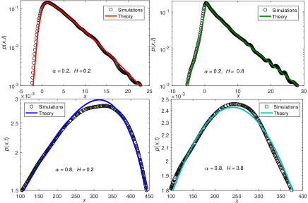
Figure 2: Simulations (dark circles) and analytical results (solid curves) from Eq. (6) for the PDF of subordinated FBM with drift $v=1$ at time $t=1000$ for varying Hurst exponents $H$ and stability indices $\alpha$. The elementary time step in the simulations was $dt=0.1$.

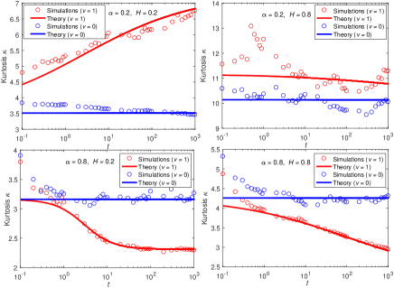
Figure 3: Simulations (circles) and theoretical results (solid curves) based on Eqs. (14) and (15) of the kurtosis for the subordinated FBM with the drift $v=1$ and without drift $v=0$ for varying values of Hurst exponent $H$ and stability index $\alpha$ with increasing time. The elementary time step in the simulations was $dt=0.1$.

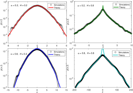
Figure S1: Simulations (dark circles) and analytical results (solid curves) from Eq. (7) for the PDF of subordinated FBM without drift ($v=0$) and for different $H$ and $\alpha$, for $t=1000$.

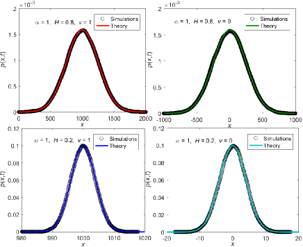
Figure S5: Simulations (dark circles) and analytical results (solid curves) from Eq. (6) for the PDF of subordinated FBM with drift $v=1$ and without drift ($v=0$) for different $H$ and for $\alpha=1$ at $t=1000$.

In Fig. 2 we show the results of our analytical calculations and stochastic simulations of the PDF with drift $v=1$ at time $t=1000$ for the Hurst exponents $H=0.2$ and $H=0.8$, and stability indices $\alpha=0.2$ and $\alpha=0.8$. The analytical results agree nicely with the simulations for all cases, apart from deviations aorund the maxima for the case $\alpha=0.8$. The PDFs are asymmetric as compared with the symmetric PDFs of subordinated FBM without drift in Fig. S1 (see App. A). All PDFs have distint cusp-like peaks for smaller $\alpha$ both in the presence and absence of drift. The PDFs of subordinated FBM with $\alpha=1$ (i.e., the operational time has the same mean behavior as the process time) are shown in Fig. S5 (App. A).

To check the non-Gaussianity of the PDF for subordinated FBM with drift, we illustrate in Fig. 3 the kurtosis based on Eqs. (14) and (15) with the drift $v=1$ and without drift ($v=0$) from analytical calculations and simulations, as function of time. For different values of $H$ and $\alpha$ the general agreement is good. However, due to the fourth order of the means entering the kurtosis, we did not manage to achieve a higher numerical accuracy from our simulations. The results for the kurtosis, whose value for a Gaussian in one dimension is $\kappa=3$, indicate that the PDFs are non-Gaussian, which is in full agreement with the results given in Figs. 2 and S1 (App. A). We note specifically that for smaller values of $\alpha$ or larger value of $H$, the values of the kurtosis exhibit values that are much larger than the Gaussian value 3.

IV Time averaged mean squared displacement and its distribution

The TAMSD is defined as he ; metz14 ; pt1 ; bark12

$$\overline{\delta^{2}(\Delta)}=\frac{1}{T-\Delta}\int_{0}^{T-\Delta}[x(t+\Delta)-x(t)]^{2}dt,$$ (17)

where $T$ is the measurement time and $\Delta$ is called the lag time. The average TAMSD is based on the autocorrelation function $\langle x(t_{1})x(t_{2})\rangle$, which is given by

$$\langle x(t_{1})x(t_{2})\rangle = \int_{0}^{\infty}\int_{0}^{\infty}\langle x(s_{1})x(s_{2})\rangle h(s_{2},t_{2},s_{1},t_{1})ds_{1}ds_{2}$$ (18)

$$= \int_{0}^{\infty}\int_{0}^{\infty}\left[v^{2}s_{1}s_{2}+\frac{1}{2}\left(s_{1}^{2H}+s_{2}^{2H}-|s_{2}-s_{1}|^{2H}\right)\right]h(s_{2},t_{2};s_{1},t_{1})ds_{1}ds_{2}$$

$$= v^{2}\langle s(t_{1})s(t_{2})\rangle+\frac{1}{2}\left[\langle s(t_{1})^{2H}\rangle+\langle s(t_{2})^{2H}\rangle-\langle|s(t_{2})-s(t_{1})|^{2H}\rangle\right].$$

As we argued in Sec. II, $s(t)$ is the hitting time, also called the number of steps up to time $t$. Therefore

$$\langle[x(t_{2})-x(t_{1})]^{2}\rangle=\langle x^{2}(t_{2})\rangle+\langle x^{2}(t_{1})\rangle-2\langle x(t_{1})x(t_{2})\rangle=v^{2}\langle[s(t_{2})-s(t_{1})]^{2}\rangle+\langle|s(t_{2})-s(t_{1})|^{2H}\rangle.$$ (19)

Let $t_{1}=t$ and $t_{2}=t+\Delta$, then the fractional moment of order $\vartheta$ of $s(t_{2})-s(t_{1})$ is fox

$$\langle[s(t+\Delta)-s(t)]^{\vartheta}\rangle=\frac{\Gamma(1+\vartheta)}{\Gamma(\alpha)\Gamma(2-\alpha+\alpha\vartheta)}\,_{2}F_{1}\left(1,1-\alpha;2-\alpha+\alpha\vartheta;-\frac{\Delta}{t}\right)\frac{\Delta^{1-\alpha+\alpha\vartheta}}{t^{1-\alpha}},$$ (20)

where ${}_{2}F_{1}$ is the hypergeometric function. With the help of Eqs. (17) and (20) we obtain the mean TAMSD in the form

$$\left<\overline{\delta^{2}(\Delta)}\right> = \frac{1}{T-\Delta}\int_{0}^{T-\Delta}\left(\frac{2v^{2}}{\Gamma(\alpha)\Gamma(2+\alpha)}\,_{2}F_{1}\left(1,1-\alpha;2+\alpha;-\frac{\Delta}{t}\right)\frac{\Delta^{1+\alpha}}{t^{1-\alpha}}\right.$$ (21)

$$\left.+\frac{\Gamma(1+2H)}{\Gamma(\alpha)\Gamma(2-\alpha+2H\alpha)}\,_{2}F_{1}\left(1,1-\alpha;2-\alpha+2H\alpha;-\frac{\Delta}{t}\right)\frac{\Delta^{1-\alpha+2H\alpha}}{t^{1-\alpha}}\right)dt.$$

In the limit $\Delta\ll t$ we have ${}_{2}F_{1}(1,1-\alpha;2-\alpha+\alpha\vartheta;0)\sim 1$ virch , then Eq. (21) becomes

$$\left<[x(t_{2})-x(t_{1})]^{2}\right>\sim\frac{2}{\Gamma(\alpha)\Gamma(2+\alpha)}\frac{v^{2}\Delta^{1+\alpha}}{t^{1-\alpha}}+\frac{\Gamma(1+2H)}{\Gamma(\alpha)\Gamma(2-\alpha+2H\alpha)}\frac{\Delta^{1-\alpha+2H\alpha}}{t^{1-\alpha}}.$$ (22)

Performing the temporal integration in Eq. (17) we get

$$\left<\overline{\delta^{2}(\Delta)}\right>\sim\frac{2v^{2}}{\alpha\Gamma(\alpha)\Gamma(2+\alpha)}\frac{\Delta^{1+\alpha}}{T^{1-\alpha}}+\frac{\Gamma(1+2H)}{\alpha\Gamma(\alpha)\Gamma(2-\alpha+2H\alpha)}\frac{\Delta^{1-\alpha+2H\alpha}}{T^{1-\alpha}}.$$ (23)

In the limit $\Delta\gg t$, we have ${}_{2}F_{1}\left(1,1-\alpha;2-\alpha+\alpha\vartheta;-\frac{\Delta}{t}\right)\sim\left(\frac{t+\Delta}{t}\right)^{-(1-\alpha)}\frac{\Gamma(2-\alpha+\alpha\vartheta)\Gamma(\alpha)}{\Gamma(1+\alpha\vartheta)}$, and Eq. (21) becomes

$$\left<[x(t_{2})-x(t_{1})]^{2}\right>\sim\frac{2v^{2}}{\Gamma(1+2\alpha)}\left(\Delta^{2}+(\alpha-1)t\Delta^{2\alpha-1}\right)+\frac{\Gamma(1+2H)}{\Gamma(1+2H\alpha)}\left(\Delta^{2H\alpha}+(\alpha-1)t\Delta^{2H\alpha-1}\right).$$ (24)

Similarly from Eq. (17) we get

$$\left<\overline{\delta^{2}(\Delta)}\right>\sim\frac{2v^{2}}{\Gamma(1+2\alpha)}\left(\Delta^{2}+\frac{(\alpha-1)(T-\Delta)\Delta^{2\alpha-1}}{2}\right)+\frac{\Gamma(1+2H)}{\Gamma(1+2H\alpha)}\left(\Delta^{2H\alpha}+\frac{(\alpha-1)(T-\Delta)\Delta^{2H\alpha-1}}{2}\right).$$ (25)

We note that subordinated FBM with drift for the limit $\alpha=1$ is an ergodic stochastic process deng ; schw ; jae_pre12 .

Fig. 4 shows results from simulations of the MSD, a number of individual TAMSDs, and the mean TAMSD for subordinated FBM with drift $v=1$ for different values of $H$ and $\alpha$. In Fig. 4 the analytical results are in nice agreement with the simulations for the MSD and the mean TAMSD. We also note that individual TAMSDs show a wide spread, especially for smaller values of $\alpha$, consistent with the weakly non-ergodic behavior of CTRW motion he ; bark12 ; pt1 ; metz14 . The values of the MSD and TAMSD grow faster with time for subordinated FBM with drift as compared to the same motion in absence of the drift, as shown in Fig. S2 (App. A).

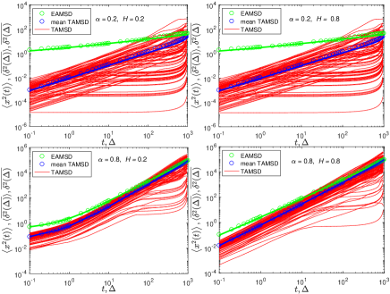
Figure 4: MSD (green circles), a number of individual TAMSDs (thin red curves), and the mean TAMSD (thick blue circles) for subordinated FBM with drift $v=1$ and different values of $H$ and $\alpha$. Theoretical results for the MSD (thick solid green curves) and mean TAMSD (thick solid blue curves) as given in Eqs. (9) and (21), respectively, show nice agreement. Parameters: length of the trajectories $T=1000$, elementary time-step $dt=0.1$, and number of trajectories $n=300$.

To quantify the relative amplitude spread of individual TAMSD, we use the dimensionless variable he ; bark12 ; metz14

$$\xi(\Delta)=\frac{\overline{\delta^{2}(\Delta)}}{\left<\overline{\delta^{2}(\Delta)}\right>}.$$ (26)

The values of $\xi$ fluctuate around the mean value $\left<\xi(\Delta)\right>=1$. The corresponding PDF $\phi(\xi)$ can be expressed as modified totally asymmetric Lévy stable density he ; metz14 or via the Mittag-Leffler function needcite . The variance $\mathrm{EB}=\langle\xi^{2}\rangle-1$ is called the ergodicity breaking parameter he ; bark12 ; metz14 ; pt1 .

Fig. 5 illustrates the scatter PDF of the TAMSD for the same parameters as in Fig. 4 for the three different lag times $\Delta=0.1$, $1$, and $10$. The results show that the distributions are not symmetric around the mean $\left<\xi(\Delta)\right>=1$, and have a spike and long heavy tail for smaller values of $\alpha$. It is also noted that for smaller values of $\alpha$ the particles will have longer average waiting times, and thus the probability will be higher for trajectories without any displacement up to $T$, $\xi(\Delta)=0$, which agrees well with the general observed trends in Fig. 4 (see also the discussions in he ; metz14 ; fox ). The simulations of the scatter PDF for subordinated FBM without drift have similar statistical properties, see Fig. S3 (App. A).

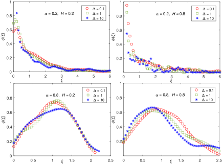
Figure 5: Amplitude scatter PDF $\phi(\xi)$ of TAMSDs for subordinated FBM with drift $v=1$ and varying values of $H$ and $\alpha$. The symbols (circle, square, and star) respectively denote simulations with the lag time $\Delta=0.1$, $1$, and $10$.

V Discussion

We studied subordinated FBM in the presence of a constant external drift, combining long-range correlated Gaussian motion characterized by a Hurst exponent $H$ and long-tailed, scale-free PDFs of immobilization (waiting) times with scaling exponent $\alpha$. As expected, at long times the drift term dominates the transport behavior, which we quantified in terms of the ensemble- and time-averaged moments as well as the PDF. Technically, we employ the subordination approach based on a stable subordinator. This transforms the "operational time" of the parental FBM to the "process time" of the combined motion in the presence of the immobilization events. The resulting process, studied in fox in the absence of drift, thus combines two central properties of stochastic motion observed in a wide range of experiments. Currently, such observations predominantly come from single-particle tracking in soft- and bio-matter manz ; jaqa ; etoc or large-scale computer simulations, see, e.g., amanda ; jeon . Given the development of experimental methods to record single-particle movement in geophysical contexts hard ; roub , it will be interesting to see whether similarly rich behaviors are unveiled in this context.

In our analysis we highlighted the different scaling behaviors in the MSDs due to diffusion and drift, respectively. The resulting PDF is non-Gaussian, and we showed how $H$ and $\alpha$ influence the shape parameters (skewness and kurtosis). We also studied from simulations the amplitude scatter of individual TAMSDs. In future work we will also consider aging effects, for which explicit expressions for the ensemble-and time-averaged moments will be obtained.

Subordinated FBM as studied in fox in absence of a drift and with a drift as investigated herein, complements similar combined stochastic processes reported in literature. We here mention the combination of CTRWs on fractal structures such as a Sierpiński gasket mero , the conspiracy of FBM with scaled Brownian motion (SBM) andreywei in which the diffusion coefficient is a power-law function of time lim ; jae , and the combination of FBM with a stochastically evolving ("diffusing") diffusivity wei ; wei1 . Such processes will form the basis for future extensions of data analyses based on statistical observables (such as those developed herein), Bayesian maximum likelihood approaches michael ; samu ; samu1 , or machine-learning strategies janusz ; janusz1 ; bo ; yael ; gorka ; andi ; henrik .

Appendix A Supplementary figures

We here present additional figures complementing the behaviors presented in the main text.

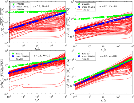
Figure S2: MSD (green circles), individual TAMSDs (thin red curves), and mean TAMSD (thick blue circles) for subordinated FBM without drift ($v=0$) for different $H$ and $\alpha$. Theoretical results for the MSD (thick solid green curves) and mean TAMSD (thick solid blue curves) are based on Eqs. (9) and (21), respectively. Parameters: trajectory length $T=1000$, elementary time-step $dt=0.1$, and number of trajectories $n=300$.

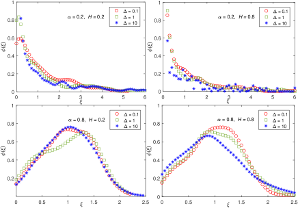
Figure S3: Amplitude scatter PDF of TAMSDs for subordinated FBM without drift ($v=0$) for different $H$ and $\alpha$. The symbols (circle, square, and star) respectively denote simulations with lag time $\Delta=0.1$, $1$, and $10$.

References

- (1) N. G. van Kampen, Stochastic processes in physics and chemistry (North-Holland, Amsterdam, 1981).
- (2) P. Hänggi and F. Marchesoni, Introduction: 100 years of Brownian motion, Chaos 15, 026101 (2005).
- (3) J. Spiechowicz, I. G. Marchenko, P. Hänggi, and J. Łuczka, Diffusion coefficient of a Brownian particle in equilibrium and nonequilibrium: Einstein model and beyond, E-print arXiv:2211.14190.
- (4) P. Lévy, Processus stochastiques et mouvement brownien (Gauthier-Villars, Paris, 1965).
- (5) R. Metzler and J. Klafter, The random walk’s guide to anomalous diffusion: A fractional dynamics approach, Phys. Rep. 339, 1-77 (2000).
- (6) J. P. Bouchaud and A. Georges, Anomalous diffusion in disordered media: Statistical mechanisms, models and physical applications, Phys. Rep. 195, 127 (1990).
- (7) R. L. Magin, C. Ingo, L. Colon-Perez, W. Triplett, and T. H. Mareci, Characterization of anomalous diffusion in porous biological tissues using fractional order derivatives and entropy, Micropor. Mesopor. Mat. 178, 39 (2013).
- (8) H. Sun, M. Meerschaert, Y. Zhang, J. Zhu, and W. Chen, A fractal Richards’ equation to capture the non-Boltzmann scaling of water transport in unsaturated media, Adv. Water Resour. 52, 292 (2013).
- (9) D. Bolster, D. Benson, M. Meerschaert, and B. Baeumer, Mixing-driven equilibrium reactions in multidimensional fractional advection-dispersion systems, Physica A 392, 2513 (2013).
- (10) R. Metzler, J.-H. Jeon, A. G. Cherstvy, and E. Barkai, Anomalous diffusion models and their properties: Non-stationarity, non-ergodicity, and ageing at the centenary of single particle tracking, Phys. Chem. Chem. Phys. 16, 24128 (2014).
- (11) I. M. Sokolov, Models of anomalous diffusion in crowded environments, Soft Matter 8, 9043 (2012).
- (12) E. Barkai, Y. Garini, and R. Metzler, Strange kinetics of single molecules in living cells, Phys. Today 65(8), 29 (2012).
- (13) I. Golding and E. C. Cox, Physical nature of bacterial cytoplasm, Phys. Rev. Lett. 96, 098102 (2006).
- (14) S. C. Weber, A. J. Spakowitz, and J. A. Theriot, Bacterial chromosomal loci move subdiffusively through a viscoelastic cytoplasm, Phys. Rev. Lett. 104, 238102 (2010).
- (15) J.-H. Jeon, V. Tejedor, S. Burov, E. Barkai, C. Selhuber-Unkel, K. Berg-Sørensen, L. Oddershede, and R. Metzler, In vivo anomalous diffusion and weak ergodicity breaking of lipid granules, Phys. Rev. Lett. 106, 048103 (2011).
- (16) J. Szymanski and M. Weiss, Elucidating the origin of anomalous diffusion in crowded fluids, Phys. Rev. Lett. 103, 038102 (2009).
- (17) J-.H. Jeon, N. Leijnse, L. Oddershede, and R. Metzler, Anomalous diffusion and power-law relaxation in wormlike micellar solution, New J. Phys. 15, 045011 (2013).
- (18) D. Krapf and R. Metzler, Strange interfacial molecular dynamics, Phys. Today 72(9), 48 (2019).
- (19) G. Seisenberger, M. U. Ried, T. Endreß, H. Büning, M. Hallek, and C. Bräuchle, Real-time single-molecule imaging of the infection pathway of an adeno-associated virus, Science 294, 1929 (2001).
- (20) M. S. Song, H. C. Moon, J.-H. Jeon, and H. Y. Park, Neuronal messenger ribonucleoprotein transport follows an aging Lévy walk, Nat. Commun. 9, 344 (2018).
- (21) J. F. Reverey, J.-H. Jeon, H. Bao, M. Leippe, R. Metzler, and C. Selhuber-Unkel, Superdiffusion dominates intracellular particle motion in the supercrowded space of pathogenic Acanthamoeba castellanii, Sci. Rep. 5, 11690 (2015).
- (22) D. Robert, T. H. Nguyen, F. Gallet, and C. Wilhelm, In vivo determination of fluctuating forces during endosome trafficking using a combination of active and passive microrheology, PLoS One 5, e10046 (2010).
- (23) Y. Meroz and I. M. Sokolov, A toolbox for determining subdiffusive mechanisms, Phys. Rep. 573, 1 (2015).
- (24) E. Aghion, P. G. Meyer, V. Adlakha, H. Kantz, and K. E. Bassler, Moses, Noah, and Joseph effects in Lévy walks, New J. Phys. 23, 023002 (2021).
- (25) O. Vilk, E. Aghion, T. Avgar, C. Beta, O. Nagel, A. Sabri, R. Sarfati, D. K. Schwartz, M. Weiss, D. Krapf, R. Nathan, R. Metzler, and M. Assaf, Unravelling the origins of anomalous diffusion: from molecules to migrating storks, Phys. Rev. Res. 4, 033055 (2022).
- (26) M. Magdziarz, A. Weron, K. Burnecki, and J. Klafter, Fractional Brownian motion versus the continuous-time random walk: A simple test for subdiffusive dynamics, Phys. Rev. Lett. 103, 18 (2009).
- (27) J. Krog and M. A. Lomholt, Bayesian inference with information content model check for Langevin equations, Phys. Rev. E 96, 062106 (2017).
- (28) S. Thapa, M. A. Lomholt, J. Krog, A. G. Cherstvy, and R. Metzler, Bayesian nested sampling analysis of single particle tracking data: maximum likelihood model selection applied to stochastic diffusivity data, Phys. Chem. Chem. Phys. 20, 29018 (2018).
- (29) A. G. Cherstvy, S. Thapa, C. E. Wagner, and R. Metzler, Non-Gaussian, non-ergodic, and non-Fickian diffusion of tracers in mucin hydrogels, Soft Matter 15, 2526 (2019).
- (30) G. Muñoz-Gil, M. A. Garcia-March, C. Manzo, J. D. Martín-Guerrero, and M. Lewenstein, Single trajectory characterization via machine learning, New J. Phys. 22, 013010 (2020).
- (31) N. Granik, L. E. Weiss, E. Nehme, M. Levin, M. Chein, E. Perlson, Y. Roichman, and Y. Shechtman, Single-Particle diffusion characterization by deep learning, Biophys. J. 117, 185 (2019).
- (32) J. Janczura, P. Kowalek, H. Loch-Olszewska, J. Szwabiñski, and A. Weron, Classification of particle trajectories in living cells: machine learning versus statistical testing hypothesis for fractional anomalous diffusion, Phys. Rev. E 102, 3 (2020).
- (33) P. Kowalek, H. Loch-Olszewska, Ł. Łaszczuk, J. Opała, and J. Szwabiński, Boosting the performance of anomalous diffusion classifiers with the proper choice of features, J. Phys. A 55, 24 (2022).
- (34) S. Bo, F. Schmidt, R. Eichhorn, and G. Volpe, Measurement of anomalous diffusion using recurrent neural networks, Phys. Rev. E, 100,1 (2019).
- (35) G. Muñoz-Gil, G. Volpe, M. A. Garcia-March, E. Aghion, A. Argun, C. B. Hong, T. Bland, S. Bo, J. A. Conejero, N. Firbas, Ò. Garibo i Orts, A. Gentili, Z. Huang, J.-H. Jeon, H. Kabbech, Y. Kim, P. Kowalek, D. Krapf, H. Loch-Olszewska, M. A. Lomholt, J.-B. Masson, P. G. Meyer, S. Park, B. Requena, I. Smal, T. Song, J. Szwabiński, S. Thapa, H. Verdier, G. Volpe, A. Widera, M. Lewenstein, R. Metzler, and C. Manzo, Objective comparison of methods to decode anomalous diffusion, Nature Comm. 12, 6253 (2021).
- (36) H. Seckler and R. Metzler, Bayesian deep learning for error estimation in the analysis of anomalous diffusion, Nature Comm. 13, 6717 (2022).
- (37) A. N. Kolmogorov, The local structure of turbulence in an incompressible fluid at very high Reynolds numbers, Dokl. Acad. Nauk USSR 30, 299 (1940).
- (38) B. B. Mandelbrot and J. W. van Ness, Fractional Brownian motions, fractional noises and applications, SIAM Rev. 10, 422 (1968).
- (39) J. H. Jeon, M. S. Monne, M. Javanainen, and R. Metzler, Anomalous diffusion of phospholipids and cholesterols in a lipid bilayer and its origins, Phys. Rev. Lett. 109, 188103 (2012).
- (40) D. Krapf, N. Lukat, E. Marinari, R. Metzler, G. Oshanin, C. Selhuber-Unkel, A. Squarcini, L. Stadler, M. Weiss, and X. Xu, Spectral content of a single non-Brownian trajectory, Phys. Rev. X 9, 011019 (2019).
- (41) S. Janušonis, N. Detering, R. Metzler, and T. Vojta, Serotonergic axons as fractional Brownian motion paths: Insights into the self-organization of regional densities, Front. Comput. Neurosci. 14, 56 (2020).
- (42) E. W. Montroll and G. H. Weiss, Random walks on lattices. II, J. Math. Phys. 6, 167 (1965).
- (43) H. Scher and E. W. Montroll, Anomalous transit-time dispersion in amorphous solids, Phys. Rev. B 12, 2455 (1975).
- (44) M. Schubert, E. Preis, J. C. Blakesley, P. Pingel, U. Scherf, and D. Neher, Mobility relaxation and electron trapping in a donor/acceptor copolymer, Phys. Rev. E 87, 024203 (2013).
- (45) A. V. Weigel, B. Simon, M. M. Tamkun, and D. Krapf, Ergodic and nonergodic processes coexist in the plasma membrane as observed by single-molecule tracking, Proc. Natl. Acad. Sci. USA 108, 6438 (2011).
- (46) O. Rubner and A. Heuer, From elementary steps to structural relaxation: A continuous-time random-walk analysis of a supercooled liquid, Phys. Rev. E 78, 011504 (2008).
- (47) A. Díez Fernandez, P. Charchar, A. G. Cherstvy, R. Metzler, and M. W. Finnis, The diffusion of doxorubicin drug molecules in silica nanochannels is non-Gaussian and intermittent, Phys. Chem. Chem. Phys. 22, 27955 (2020).
- (48) B. Berkowitz, A. Cortis, M. Dentz, and H. Scher, Modeling non-Fickian transport in geological formations as a continuous time random walk, Rev. Geophys. 44, RG2003 (2006).
- (49) S. M. A. Tabei, S. Burov, H. Y. Kima, A. Kuznetsov, T. Huynh, J. Jureller, L. H. Philipson, A. R. Dinner, and N. F. Scherer, Intracellular transport of insulin granules is a subordinated random walk, Proc. Natl Acad. Sci. USA 110, 4911 (2013).
- (50) A. Mosqueira, P. A. Camino, and F. J. Barrantes, Cholesterol modulates acetylcholine receptor diffusion by tuning confinement sojourns and nanocluster stability, Sci. Rep. 8, 1 (2018).
- (51) F. Etoc, E. Balloul, C. Vicario, D. Normanno, J. Piehler, M. Dahan, and M. Coppey, Non-specific interactions govern cytosolic diffusion of nanosized objects in mammalian cells, Nature Mat. 17, 740 (2018).
- (52) Z. R. Fox, E. Barkai, and D. Krapf, Aging power spectrum of membrane protein transport and other subordinated random walks, Nat. Commun. 12, 6162 (2021).
- (53) D. Applebaum, Lévy Processes and Stochastic Calculus, Cambridge Studies in Advanced Mathematics, Cambridge University Press, Cambridge, 2009.
- (54) S. Bochner. Subordination of non-Gaussian stochastic processes, Proc Natl Acad Sci USA 48, 19 (1962).
- (55) W. Feller. An introduction to probability theory and its applications, Wiley, New York Wiley, 1971.
- (56) A. Chechkin and I. M. Sokolov, Relation between generalized diffusion equations and subordination schemes, Phys. Rev. E 103, 032133 (2021).
- (57) M. M. Meerschaert and P. Straka, Inverse stable subordinators, Math. Model. Nat. Phenom. 8, 1 (2013).
- (58) M. M. Meerschaert and H.-P. Scheffler, Limit theorems for continuous-time random walks with infinite mean waiting times, J. Appl. Probab. 41, 623 (2004).
- (59) X. Wang and Y. Chen, Ergodic property of random diffusivity system with trapping events, Phys. Rev. E 105, 014106 (2022).
- (60) M. Magdziarz, A. Weron and K. Weron, Fractional Fokker-Planck dynamics: Stochastic representation and computer simulation, Phys. Rev. E 75, 016708 (2007).
- (61) H. C. Fogedby, Langevin equations for continuous time Lévy flights, Phys. Rev. E 50, 1657 (1994).
- (62) W. Gawronski, Asymptotic forms for the derivatives of one-sided stable laws, Ann. Probab. 16, 1348 (1988).
- (63) K. A. Penson and K. Górska, Exact and explicit probability densities for one-sided Lévy stable distributions, Phys. Rev. Lett. 105, 210604 (2010).
- (64) A. Saa and R. Venegeroles, Alternative numerical computation of one-sided Lévy and Mittag-Leffler distributions, Phys. Rev. E 84, 026702 (2011).
- (65) K. A. Penson and K. Górska, On the properties of Laplace transform originating from one-sided Lévy stable laws, J. Phys. A: Math. Theor. 49, 065201 (2016).
- (66) G. Dattoli, K. Górska, A. Horzela, K. A. Penson, and E. Sabia, Theory of relativistic heat polynomials and one-sided Lévy distributions, J. Math. Phys. 58, 063510 (2017).
- (67) E. Barkai, Fractional Fokker-Planck equation, solution, and application, Phys. Rev. E 63, 046118 (2001).
- (68) Y. He, S. Burov, R. Metzler, and E. Barkai, Random time-scale invariant diffusion and transport coefficients, Phys. Rev. Lett. 101, 058101 (2008).
- (69) N. Virchenko, On the generalized confluent hypergeometric function and its application, Fract. Calc. Appl. Anal. 9, 101 (2006).
- (70) W. Deng and E. Barkai, Ergodic properties of fractional Brownian-Langevin motion, Phys. Rev. E 79, 011112 (2009).
- (71) M. Schwarzl, A. Godec, and R. Metzler, Quantifying nonergodicity of anomalous diffusion with higher order moments, Sci. Rep. 7, 3878 (2017).
- (72) J.-H. Jeon and R. Metzler, Inequivalence of time and ensemble averages in ergodic systems: exponential versus power-law relaxation in confinement, Phys. Rev. E 85, 021147 (2012).
- (73) D. A. Darling and M. Kac, On On Occupation Times for Markoff Processes, Trans. Amer. Math. Soc. 84, 444 (1957).
- (74) C. Manzo and M. F. Garcia-Parajo, A review of progress in single particle tracking: From methods to biophysical insights, Rep. Prog. Phys. 78, 124601 (2015).
- (75) K. Jaqaman, D. Loerke, M. Mettlen, H. Kuwata, S. Grinstein, S. L. Schmid, and G. Danuser, Robust single-particle tracking in live-cell time-lapse sequences, Nat. Methods 5, 695 (2018).
- (76) R. A. Hardy, M. R. James, J. M. Pates, and J. N. Quinton, Using real time particle tracking to understand soil particle movements during rainfall events, Catena 150, 32 (2017).
- (77) D. Roubinet, J.-R. De Dreuzy, and D. M. Tartakovsky, Particle-tracking simulations of anomalous transport in hierarchically fractured rocks, Comput. Geosci. 50, 52 (2013).
- (78) Y. Meroz, I. M. Sokolov, and J. Klafter, Subdiffusion of mixed origins: When ergodicity and nonergodicity coexist, Phys. Rev. E 81, 010101 (2010).
- (79) W. Wang, R. Metzler, and A. G. Cherstvy, Anomalous diffusion, aging, and nonergodicity of scaled Brownian motion with fractional Gaussian noise: overview of related experimental observations and models, Phys. Chem. Chem. Phys. 24, 18482 (2022).
- (80) S. C. Lim and S. V. Muniandy, Self-similar Gaussian processes for modeling anomalous diffusion, Phys. Rev. E 66, 021114 (2002).
- (81) J-.H. Jeon, A. V. Chechkin, and R. Metzler, Scaled Brownian motion: a paradoxical process with a time dependent diffusivity for the description of anomalous diffusion, Phys. Chem. Chem. Phys. 16, 15811 (2014).
- (82) W. Wang, A. G. Cherstvy, A. V. Chechkin, S. Thapa, F. Seno, X. Liu, and R. Metzler, Fractional Brownian motion with random diffusivity: emerging residual nonergodicity below the correlation time, J. Phys. A 53, 474001 (2020).
- (83) W. Wang, F. Seno, I. M. Sokolov, A. V. Chechkin, and R. Metzler, Unexpected crossovers in correlated random-diffusivity processes, New J. Phys. 22, 083041 (2020).