Hierarchical Generative Adversarial Imitation Learning with Mid-level Input Generation for Autonomous Driving on Urban Environments

Abstract

Deriving robust control policies for realistic urban navigation scenarios is not a trivial task. In an end-to-end approach, these policies must map high-dimensional images from the vehicle’s cameras to low-level actions such as steering and throttle. While pure Reinforcement Learning (RL) approaches are based exclusively on rewards, Generative Adversarial Imitation Learning (GAIL) agents learn from expert demonstrations while interacting with the environment, which favors GAIL on tasks for which a reward signal is difficult to derive. In this work, the hGAIL architecture was proposed to solve the autonomous navigation of a vehicle in an end-to-end approach, mapping sensory perceptions directly to low-level actions, while simultaneously learning mid-level input representations of the agent’s environment. The proposed hGAIL consists of an hierarchical Adversarial Imitation Learning architecture composed of two main modules: the GAN (Generative Adversarial Nets) which generates the Bird’s-Eye View (BEV) representation mainly from the images of three frontal cameras of the vehicle, and the GAIL which learns to control the vehicle based mainly on the BEV predictions from the GAN as input. Our experiments have shown that GAIL exclusively from cameras (without BEV) fails to even learn the task, while hGAIL, after training exclusively on one city, was able to autonomously navigate successfully in 98% of the intersections of a new city not used in training phase.

I Introduction

Commonly, Autonomous Driving (AD) has been implemented using individual modules for perception, planning and control organized in a pipeline [1, 2, 3, 4]. However, learning approaches have been on the rise, in an attempt to tackle the complexities of AD in different scenarios, in simulation or even in the real world. Most of the approaches are based on Behavior Cloning (BC), which uses supervised learning on a set of expert demonstrations collected offline [5, 6, 7, 8, 9], e.g., with a human driver generating a set of input (observations) and corresponding desired output pairs. The latter approach suffers from covariate shift [10, 11, 12], since it can not teach robustly the learning agent a trajectory which does not accumulate errors.

Reinforcement Learning (RL) approaches to AD can learn policies that do not present this covariate shift issue, since the agent is able to learn in interaction with the environment, considering the whole sample trajectories and not only independent observation-action samples as in BC. However, RL requires the definition of a reward signal, which can be cumbersome to do it considering the complexity of a driver’s behavior and its environment. Although Inverse RL can be used for imitation learning purposes [13], it is expensive to run since it executes RL in a loop. Learning in IRL is computationally more expensive than just learning a policy directly from expert demonstrations.

On the other hand, Generative Adversarial Imitation Learning (GAIL) [14] provides a way to train agents in interaction with their environments, directly from expert demonstrations. This approach has been validated in the CARLA simulator for autonomous driving in urban scenarios previously [15], showing it can scale to large environments. However, in [15] only fixed routes were considered. Although the agent’s architecture was general enough for dynamic routes, with inputs such as the high-level command and the next point of the sparse trajectory in the vehicle’s reference frame, the network had limitations for learning a general policy for dynamic routes, i.e., those that can change on the fly (turn left, right, or go straight at an intersection) from the perspective of the agent.

In order to facilitate the agent learning task, intermediate sensory representations can be employed. For instance, Bird’s-Eye View (BEV) representations of the road ahead of the vehicle have been used as mid-level input to trajectory generation and motor control networks in [7] and [16], respectively. BEV requires access to maps in order to map frontal camera images, pedestrians and traffic lights into the required abstract BEV image. One of the advantages of such approach is enabling transfer to real-world by a relatively easy process: it requires mapping the real-world images to the same abstract representation used to train the agent in simulation. Besides, training agents with mid-level visual inputs such as BEV and others (e.g., optical flow, depth, semantic segmentation, and albedo) make policies learn faster, generalize better and achieve higher task performance [17]. Other works employ semantic segmentation for semantic driving [18, 19, 20], offering supporting evidence that mid-level inputs to agents are useful for realistic downstream active tasks [17].

So far, BEV has been employed for autonomous driving in urban scenarios in [16] and [7]. However, they generate BEV input by using an algorithm which has to access a known map of the city. In contrast, in our work, we consider a mid-level BEV input, feeding the agent’s policy, that is learned simultaneously with the policy. For that, we use Conditional Generative Adversarial Nets (GANs) [21] and U-nets to map the images obtained from three frontal vehicle’s cameras to the mid-level BEV input. Thus, our agent’s architecture is formed by two main modules: one with two GAN nets that generate the mid-level BEV input which, in turn, is fed to the other module with two GAIL networks. The latter output steer, acceleration and break signals to drive the vehicle. Thus, although our agent produces a mid-level representation, it still pertains to the class of end-to-end models. The GAIL module’s cost function is augmented with a behavior cloning loss [22] in order to stabilize the policy learning. Both GAN and GAIL networks learn simultaneously, though with their own cost functions, while the agent interacts with the CARLA simulation environment for urban driving. This approach ensures that both the policy and representation networks are trained using on-policy data, learning from the agent’s mistakes.

This work contributes by:

1. proposing an end-to-end hierarchical architecture based on both GAN and GAIL for autonomous urban driving;

2. extending previous work that is applicable to fixed routes [15] to a more skilled agent able to follow dynamic routes, making the vehicle able to change the route on the fly;

3. generating BEV mid-level representations using GANs based on the input from the frontal camera images, sparse trajectory and high-level command, whose learning occurs simultaneously with the policy online learning.

II Related Works

II-A Behavior Cloning

The authors of works [8] and [9] utilized behavior cloning (BC) to learn the complex task of autonomous driving (AD) in the CARLA realistic simulator. A large dataset of human driving was collected and augmented using image processing techniques to train end-to-end policies conditioned on the desired route. Further advancements in BC were made in [23], which used a large deep ResNet network for feature extraction and fused data from camera, LiDAR, and radar to generate feature maps. The work also incorporated a probabilistic motion planner to account for uncertainties in the trajectory.

II-B Reinforcement Learning

Reinforcement learning (RL) offers the agent the opportunity to learn from interactions with the environment, rather than being limited to expert experience and performance. However, this also presents challenges such as the cost of interactions and the definition of a reward function to provide feedback to the agent.

An RL agent [24] was trained and tested in a 2D simulator, CARLA, and a real-world car racing task, where the vehicle needed to repeatedly complete a predefined circular trajectory. The agent was trained using a predictive world model, which substituted the environment for a 10-state horizon. The predictive world model was trained by deploying the agent to the chosen environment, reducing the necessary environment interactions for training the agent. The project highlights the potential use of auxiliary models to address the weakness of RL in needing large amounts of environment interactions.

A different autonomous driving project [16] employed reinforcement learning (RL) with a customized reward function to train an agent based on the mid-level BEV representation as input, during the first training phase. Afterwards, using the trained agent as an online expert, they trained a second agent through apprenticeship learning, but now in an end-to-end approach with input directly from the vehicle’s cameras. The method was evaluated on the CARLA, surpassing the default benchmarks trained by behavior cloning.

II-C GAIL

The authors in [25] used Generative Adversarial Imitation Learning (GAIL) with simple affordance-style features as inputs to reduce cascading errors in behavior-cloned policies and make them more robust to perturbations. Raw LiDAR readings and simple road features, such as speed and lane center offset, were mapped to turn-rate and acceleration to model human highway driving behavior in a realistic highway simulator. The experiment successfully reproduced human driver behavior while reducing the risk of collisions.

In [26], a hierarchical model-based GAIL was proposed to solve the autonomous driving problem in a differentiable simulator. The project used a graph-based search algorithm to generate the autonomous vehicle trajectory, which was combined with roadgraph points, traffic light signals, and other objects’ trajectories to form the input for the policy and discriminator transformer-based networks. The project demonstrated the advantage of using a top-level algorithm to generate the intended trajectory and feed it to a GAIL module in a hierarchical fashion.

II-D BEV Mid-level representation

Reinforcement learning enables an agent to be trained in a closed-loop fashion, resulting in more robust agents. However, this robustness comes with the cost of instabilities that prevent the use of very deep networks, such as ResNet [27]. In [28], the authors aim to decouple representation learning from the training of reinforcement learning as a solution to train agents that can process high-dimensional raw inputs, such as images from cameras.

In [29], a modular learning strategy is explored, producing an intention map that represents the vehicle’s future trajectory. This future trajectory is generated by the GAN’s generator, which is fed with an image from a monocular camera and a local map, cropped from an offline map using the GPS position. The intention map is combined with LiDAR data to generate a potential map, which is their mid-level input representation (similar to BEV), subsequently fed to a controller module trained to imitate a set of demonstration trajectories. The method is evaluated on CARLA and a real vehicle.

A similar modular approach is explored in [30], which combines a predicted bird’s-eye view representation with a pretrained trajectory of 0.5-meter resolution to serve as inputs to a mid-level policy network trained with behavior cloning. The bird’s-eye view is generated from raw images using a pretrained segmentation network, whose output is transformed by an U-net into an BEV top-down perspective. It is worth noting that our BEV generation is done by a Conditional GAN directly from raw camera images (and sparse trajectory, high-level command), opposed to [30] which uses two networks and also exclude occluded areas (by other obstacles or vehicles) from the BEV prediction.

Our work is inspired by [7], which trains an agent on CARLA to drive an autonomous vehicle using a bird’s-eye view representation generated by a data renderer module as input. This bird’s-eye view representation, like our own, contains a road and route representation from a top-down, agent-centered perspective. The agent learns from imitation learning, combining behavior cloning with data augmentation and auxiliary losses, but without closed-loop training. A similar work is [18], which uses the output of a scene segmentation network as a mid-level input representation. This enables the transfer of the agent’s policy to the real world, since a similar network can be used to generate the mid-level input from images of real scenes.

Our work is the first instance, to our knowledge, where a GAIL is trained using a mid-level input representation generated by a learning module to tackle the intricate task of autonomous driving navigation. Previous works also show that policies with mid-level representations as input can be trained on a simulator, and subsequently transferred to the real world. This is a cost-effective and safe way to perform closed-loop training of agents (since infractions during training of the agent occur in simulation only), in particular, by the GAIL method which provides an interactive learning based on expert demonstrations.

III Methods

III-A Conditional Generative Adversarial Networks - CGAN

Conditional Generative Adversarial Networks are composed of two neural networks, a discriminator D and a generator G. The function of G in a CGAN [21] is to translate an image $x$ into an image $y$ by mapping both $x$ and a random noise vector $z$ into an output image $G:\{x,z\}->y$. Both D and C seek to optimize the same objective function:

$$\mathop{\mathbb{E}}_{x,y}[\log(D(x,y))]+\mathop{\mathbb{E}}_{x,z}[\log(1-D(x,G(x,z))],$$ (1)

where G tries to minimize it, while D seeks to maximize it. As in traditional GANs, D learns to classify real images from generated ones, and G uses this output of D to direct its own learning. Notice that both D and G are conditioned on the input image $x$ that must be translated.

Additionally, a L1 distance loss function is added to the final objective, making the generator network G also learn from the true label $y$ as it would happen in a supervised learning task [21].

The L1 loss can model the low-frequency characteristics of images, while the CGAN loss is crucial for modeling high-frequency features. By classifying local patches of the image rather than the entire image, the discriminator can better capture high-frequency correctness, as the assumption is that pixels from different patches are independent.

This method, called PatchGAN [21], divides the image into multiple patches, and the discriminator classifies each patch individually. This results in a discriminator with fewer parameters and a detailed feedback for the agent

The CGAN is used in our work to generate the Bird’s-Eye View (BEV) image representation from the agent’s sensors such as frontal cameras and GPS, to be detailed later.

III-B Generative Adversarial Imitation Learning - GAIL

In Generative Adversarial Imitation Learning (GAIL) [14], basically, there are two components that are trained iteratively in a min-max game: a discriminative classifier $D$ is trained to distinguish between samples generated by the learning policy $\pi$ and samples generated by the expert policy $\pi_{E}$ (i.e., the labelled training set); and the learning policy $\pi$ is optimized to imitate the expert policy $\pi_{E}$. Thus, in this game, both $D$ and $\pi$ have opposite interests: $D$ feeds on state-action pair $(s,a)$ and its output seeks to detect whether $(s,a)$ comes from learning policy $\pi$ or expert policy $\pi_{E}$; and $\pi$ maps state $s$ to a probability distribution over actions $a$, learning this mapping by relying on $D$’s judgements on state-action samples (i.e., $D$ informs how close $\pi$ is from $\pi_{E}$). Mathematically, GAIL finds a saddle point $(\pi,D)$ of the expression:

$$\mathop{\mathbb{E}}_{\pi}[\log(D(s,a))]+\mathop{\mathbb{E}}_{\pi_{E}}[\log(1-D(s,a))]-\lambda H(\pi),$$ (2)

where $D:S\times A\rightarrow(0,1)$, $S$ is the state space, $A$ is the action space; $\pi_{E}$ is the expert policy; $H(\pi)$ is a policy regularizer controlled by $\lambda>=0$ [31]. GAIL works similarly to generative adversarial nets (GANs) [32], which was first used to learn generators of natural images. Both $D$ and $\pi$ can be represented by deep neural networks. In practice, a training iteration for $D$ uses Adam gradient-based optimization [33] to increase (2), and in the next iteration, $\pi$ is trained with any on-policy gradient method such as Proximal Policy Optimization (PPO) [34] to decrease (2). Formally, PPO minimizes the policy loss $\mathcal{L}_{P}$:

$$\mathcal{L}_{P}=-\mathop{\mathbb{E}}_{\pi}[\log(\pi_{\theta}(a|s))A_{\omega,\phi}(s,a)],$$ (3)

where: $\theta$ parametrizes the policy and $A_{\omega,\phi}(s,a)$ is the Advantage function that depends on the parametrized discriminator and value function network:

$$\begin{split}A_{\omega,\phi}(s,a)=&-\log(1-D_{\omega}(s,a))+\\ &\gamma\mathbb{E}_{s^{\prime}\sim T(s^{\prime}|s,a)}[V_{\phi}(s^{\prime})]-V_{\phi}(s),\end{split}$$ (4)

where $\omega$ and $\phi$ are deep networks that parametrize the discriminator $D_{\omega}$ and the state value function $V_{\phi}$, respectively; $\gamma$ is the discount factor; $T$ is the transition function in a Markov Decision Process; and $-\log(1-D_{\omega}(s,a))$ is the reward obtained from the discriminator $D_{\omega}$ by reward shaping [35]. Here, $V_{\phi}$ will be trained to output the expected sum of rewards starting from the state $s$ as input, and it functions as a variance reduction in (4).

In terms of implementation, it is worth noting that $D_{\omega}(s,a)$ in (4) assumes an sigmoid activation function, which has an image in $[0,1]$, while the activation function for $D_{\omega}(s,a)$ when training the discriminator corresponds to the hyperbolic tangent function with image in $[-1,1]$.

III-C BC-augmented GAIL

III-C1 Wasserstein loss

Instead of the original loss function of GAIL given by (2), to alleviate vanishing gradient and mode collapse problems, in this work, we employ the Wasserstein distance [36] between the policy distribution and expert distribution, as also done in [35, 37]. It measures the minimum effort to move one distribution to the place of the other, yielding a better feedback signal than the Jensen-Shannon divergence, and is given by:

$$\mathop{\mathbb{E}}_{\pi_{E}}[D(s,a)]-\mathop{\mathbb{E}}_{\pi}[D(s,a)]-\lambda H(\pi)-\lambda_{2}L_{gp},$$ (5)

where: the discriminator will try to increase (5), while $\pi$ seeks to minimize it; and $L_{gp}$ is a loss that penalizes the gradient constraining the discriminator network to the 1-Lipschitz function space, according to [36].

III-C2 BC augmentation

Formally, the behavior cloning loss function can be defined as:

$$\mathcal{L}_{BC}=-\mathop{\mathbb{E}}_{\pi_{E}}[\log(\pi(a|s))]$$ (6)

The BC augmentation is constructed taking a point from a line between the behavior cloning loss $\mathcal{L}_{BC}$ and the policy loss $\mathcal{L}_{P}$ (defined in (3)), as follows:

$$\alpha\mathcal{L}_{BC}+(1-\alpha)\mathcal{L}_{P}$$ (7)

where $\alpha$ controls the participation of each term during training. Initially, as the discriminator is yet not fully trained, the behavior cloning participation should be stronger in order to direct the agent’s policy learning with more useful and informative gradients. Thus, training starts with a high $\alpha$ and proceeds by decreasing its value using a fixed decay factor. This definition and the practical implementation follows [22].

III-D Bird’s-Eye View - BEV representation

The Bird’s-Eye View (BEV) of a vehicle represents its position and movement in a top-down coordinate system [7]. The vehicle’s location, heading, and speed are represented by $p_{t}$, $\theta_{t}$, and $s_{t}$ respectively. The top-down view is defined so that the agent’s starting position is always at a fixed point within an image (the center of it). Furthermore, it is represented by a set of images of size $W\times H$ pixels, at a ground sampling resolution of $\phi$ meters/pixel. The BEV of the environment moves as the vehicle moves, allowing the agent to see a fixed range of meters in front of it. For instance, the BEV representation for the vehicle whose three frontal cameras are shown in Fig. 1 is given in Fig. 3, where the desired route, drivable area and lane boundaries form a set of three images (or a three-channel image).

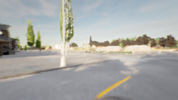
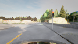
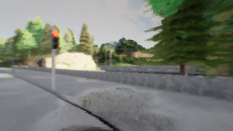
Figure 1: Images from three frontal cameras located at the left, central, and right part of the vehicle, respectively. They were taken after the first few interactions of the agent in the CARLA simulation environment Each camera produces a 256x144 RGB image.

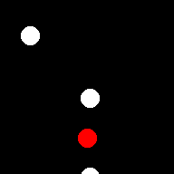
Figure 2: The sparse trajectory visual input is captured at the same frame as shown in Fig. 1. The points from the sparse trajectory and the highlighted vehicle position are plotted as circles with a radius of 10 pixels, using the same scale (pixels per meter) and perspective as the Bird’s-Eye View representation. When the image is fed to the CGAN, it is represented with only one channel and a size of 192x192 pixels.

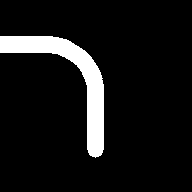
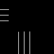
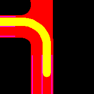
Figure 3: The three channels of the Bird’s-Eye View representation (BEV) image that our agent employs, computed at the same instant shown in Fig. 1. From left to right, the channels correspond to: desired route, drivable area, and lane boundaries. The last image shows all three channels combined in different colors.

IV Agent

Our agent’s architecture (Fig.  4) is based on hierarchical Generative Adversarial Imitation Learning (hGAIL) for training policy and mid-level representation simultaneously. There are two main parts of hGAIL: the conditional GAN that generates the BEV representation based on input from the vehicle’s frontal cameras, trajectory and high-level command; and the GAIL that learn the agent’s policy by imitation learning based on input from the BEV representation generated by the first CGAN module, current vehicle’s speed, and the last actuator values.

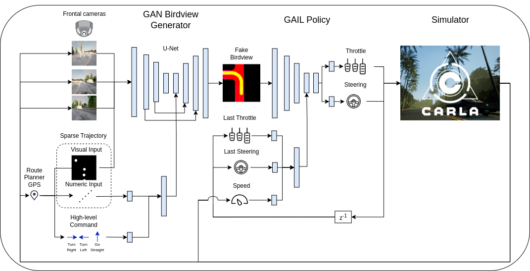
Figure 4: Hierarchical Generative Adversarial Imitation Learning (hGAIL) for policy learning with mid-level input representation. It basically consists of chained CGAN and GAIL networks, where the first one (CGAN) generates BEV representation from the vehicle’s three frontal cameras, sparse trajectory and high-level command, while the latter (GAIL) outputs the acceleration and steering based on the predicted BEV input (generated by CGAN), the current speed and the last applied actions. Both CGAN and GAIL learn simultaneously while the agent interacts to the CARLA environment. The discriminator parts of both networks are not shown for the sake of simplicity.

IV-A BEV generation with CGANs

The Conditional GAN module, used to transform the images from the frontal cameras into a top-down view representation, has two different networks named Discriminator and Generator, whose architectures can be seen in Fig. 5. In this figure, all layers from both networks are presented, and the common layers in the orange color refer to layers that exist in both networks’ architectures, even though they do not share weights (parameters).

IV-A1 Input representation

The input for the CGANs corresponds to the 192x192 resolution RGB images from the three frontal cameras represented in Fig. 1 and the sparse trajectory visual representation from Fig. 2 that are stacked to generate a 10x192x192 image, i.e., with 10 channels. The goal of the CGAN’s generator is to translate this stack of images into the 3-channel BEV representation seen in Fig. 3. In addition to this RGB input image, the discriminator also receives the 3x192x192 BEV image, which can come from either the generator as fake or from the training set as real. Other inputs to the generator are the 5 points from the sparse trajectory, one point behind the vehicle and 4 points ahead of it, represented as a vector and the high-level command as a 4-dimensional one-hot encoding vector (”lane follow”, ”left”, ”right”, ”straight”).

IV-A2 Network Architecture

Both networks’ architectures are seen in Fig. 5, where the common layers in orange refer to layers existing in both the generator and the discriminator. Notice that they are separate networks which do not share parameters: the figure was made to not repeat equivalent layers when describing both networks.

Generator

It can be seen in this figure and also in Fig. 4 that the CGAN’s generator is a U-Net [38], usually employed for image translation or segmentation. Further, while the image is processed by convolution layers, the other perceptual inputs (trajectory and command, second column in the figure) are processed by two fully connected layers followed by two transposed convolution layers which upsample their input to reach the desired resolution so that it can be merged with the last orange 256x10x10 layer in the left column. The next transposed convolution grey layer (256x22x22) merges information coming from the frontal cameras’s RGB images (left column) and the trajectory points plus the command (right command) for the generator network. Its final output is 3x192x192, corresponding to the three-channels BEV translated image.

Discriminator

The discriminator is also conditioned on the RGB images from the frontal cameras and the trajectory visual representation, which are merged to the (fake/real) BEV image, totalling 13x192x192 input to the first convolutional layer of the discriminator. The other perceptual inputs (right column) are processed similarly to the generator until it merges in a new 384x11x11 layer (in blue) with information coming from the images (256x10x10, left column). The final output corresponds to the one given by PatchGAN.

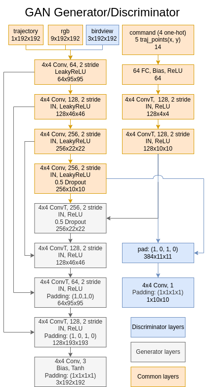
Figure 5: Conditional GAN architecture for generating the BEV input representation. The Generator and the Discriminator are separate networks which do not share parameters: the figure was made to not repeat equivalent layers when describing both networks. The generator corresponds to the U-net at the left side of Fig. 4 and aims at translating RGB 9x192x192 images from the vehicle’s frontal cameras and sparse trajectory to BEV mid-level input representation (3x192x192 images).

IV-B Policy learning with GAIL

The generator in the GAIL module iteratively seeks the $\theta$ parameters of the policy $\pi_{\theta}(.|s)$ that minimizes (7), while the discriminator seeks to maximize it. To assist the agent’s learning, loss terms for stimulating exploration are added as described after the the representations for the input, output, and architecture are presented.

IV-B1 Input representation

The input $s$ to the agent’s policy is a three-channels 192x192 image generated by the GAN network, corresponding to the mid-level BEV representation of the vehicle in its current position. In addition, the current vehicle’s speed and the last value of the policy actuators (last acceleration and steering) are also fed as input further down in the network layers (to the first fully connected layer).

IV-B2 Output representation

The vehicle in CARLA has three actuators as: $steering\in[-1,1],throttle\in[0,1]$, and $brake\in[0,1]$. Our agent’s action space is $\mathbf{a}\in[-1,1]^{2}$, where the two components of $\mathbf{a}$ correspond to steering and acceleration. Braking occurs when acceleration is negative. In this way, by modeling brake and throttle with one dimension, the agent is not allowed to brake and accelerate simultaneously [39]. Instead of using the Gaussian distribution for the policy’s actions, common choice in model-free RL, we employ the Beta distribution $\mathcal{B}(\alpha,\beta)$ due to its bounded support, which allows us to model bounded continuous action distributions, usually found in real-world applications such as autonomous driving [39], where the action space is not unbounded (i.e., the gas pedal can be actuated up to a certain limit). Besides, the policy loss $\mathcal{L}_{P}$ can be explicitly computed since clipping or squashing is not used to enforce input constraints (in the case of Gaussian distribution). Furthermore, the Beta distribution allows the policy to act in extreme situations of vehicle driving, where sharp turns and sudden braking are necessary, as its parameters $\alpha$ and $\beta$, which are defined as outputs of the policy neural network $\pi_{\theta}$ and control the shape of the distribution, can be tuned to produce such characteristic vehicle behaviors.

IV-B3 Networks’ Architectures

The agent’s policy part, which corresponds to the right side of Fig. 4, has the architecture shown in Fig. 6. The discriminator layers are also shown, even though both network’s weights are not shared, as in the previously presented CGAN architecture. The only shared part corresponds to the layers between the Generator and the value function $V_{\phi}(.)$ until the main branch splits into two heads: one for the actions steering and throttle for the generator (with 2 softplus units that outputs the $\alpha$ and $\beta$ parameters of a Beta distribution, for each action); and another for the value of state $s$, given by a linear unit. The discriminator $D(s,a)$ receives an action $a$ in addition to the observation $s$ and maps to a linear output unit, whose output value is employed as reward when training with PPO.

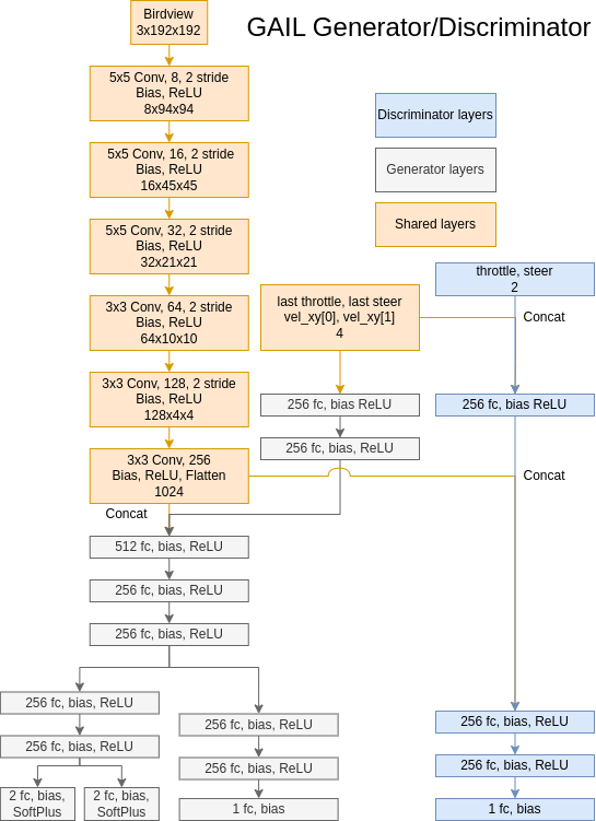
Figure 6: GAIL architecture for policy learning, corresponding to the Generator network at the right side of Fig. 4 and the Discriminator responsible for producing the reward signal. The Generator, $\pi_{\theta}(a|s)$, receives the predicted BEV image from the GAN’s generator, the last agent’s actions (throttle, steer), and the current speed as input (which forms the observation $s$ of the policy), and outputs the $\alpha$ and $\beta$ parameters of the Beta distribution for both steering and action with the SoftPlus activation function. The Value function $V_{\phi}(s)$ shares the Generator network’s layers until it branches into a separate head with more two hidden layers and a linear output unit. The Discriminator $D_{\omega}(s,a)$ receives the actions throttle and steer in addition to the observation $s$ and has a linear output unit. Notice that features from the last convolutional layer are flattened before they are merged (concat) with other information into FC (fully connected) layers.

IV-B4 Encouraring Exploration

During training, the agent is encouraged to explore the environment through two objectives, as in [16]:

$$\mathcal{L}_{\mathrm{ent}}+\mathcal{L}_{\mathrm{exp}}$$ (8)

where: the first loss function corresponds to the entropy loss commonly used to promote exploration:

$$\mathcal{L}_{\mathrm{ent}}=-\lambda_{\mathrm{ent}}\cdot\mathrm{H}(\pi_{\theta}(.|s)),$$ (9)

Minimizing $\mathcal{L}_{\mathrm{ent}}$ means maximizing entropy and thus uncertainty for the policy distribution $\pi_{\theta}$, which stimulates the agent try more diverse actions since the policy distribution for a certain state $s$ does not become too certain too quickly in the process. It also drives the action (policy) distribution towards a uniform prior (which represents maximum entropy and uncertainty) since it is equivalent to minimizing the KL-divergence to the uniform distribution defined in the support of the Beta policy $[-1,1]$:

$$\mathrm{H}(\pi_{\theta})=-\mathrm{KL}(\pi_{\theta}||\mathcal{U}(-1,1)),$$ (10)

We can also bias the agent’s learning with priors that signify meaningful behaviors for an autonomous vehicle and helps to improve and speed up the overall agent’s training from scratch. This is accomplished with the following exploration loss $\mathcal{L}_{\mathrm{exp}}$ [16]:

$$\mathcal{L}_{\mathrm{exp}}=\lambda_{\mathrm{exp}}\cdot\mathbbm{1}_{\{T-N_{z}+1,...,T\}}(k)\cdot\mathrm{KL}(\pi_{\theta}(.|s)\left|\right|p_{z}),$$ (11)

where $\mathbbm{1}$ is the indicator function and $z\in\mathcal{Z}$ is the terminal event that finishes the episode. Some examples of events in $\mathcal{Z}$ would be collision, route deviation or the car being still or blocked for too long. $\mathcal{L}_{\mathrm{exp}}$ imposes a prior $p_{z}$ to the policy during the last $N_{z}$ steps of an episode ending with one of the events in $\mathcal{Z}$. The indicator function serves as a selection mechanism of the last steps in the episode. This $p_{z}$ promotes exploration as follows: if $z$ is a collision, $p_{z}=\mathcal{B}(1,2.5)$ for the acceleration actuator, which encourages slowing down behavior; if the car is still, the acceleration prior is $p_{z}=\mathcal{B}(2.5,1)$, favoring increasing the vehicle’s speed; if the vehicle deviates from the trajectory, a uniform prior $\mathcal{B}(1,1)$ is employed for the steering actuator [16].

Thus, uniting (7) and (8), the total loss function for policy learning through PPO for our hGAIL agent is as follows:

$$\alpha\mathcal{L}_{BC}+(1-\alpha)\mathcal{L}_{P}+\mathcal{L}_{\mathrm{ent}}+\mathcal{L}_{\mathrm{exp}}$$ (12)

V Experimental Results

The goal of the vehicle is to navigate autonomously in the city shown in Fig. 7 using the hGAIL agent’s architecture with mid-level BEV input generation .

V-A Collected data

The environment and trajectories are obtained from the CARLA Leaderboard evaluation platform . In particular, the town01 environment from this platform along with ten predefined trajectories are employed to generate the expert training set.

The expert dataset is constructed using a deterministic agent that navigates using a dense point trajectory and a classic PID controller [40]. The dense point trajectory provides many points at a fine resolution, whereas a sparse point trajectory consists of considerably fewer points, providing only a general sense of direction to the agent. As a result, the dense point trajectory is utilized to generate training data by the expert, whereas the sparse point trajectory is employed by the agent for more general guidance.

In Fig. 7, one of the 10 routes executed by the expert to form the labeled training set of demonstrations is shown, where the line starting in yellow and ending in red represents the desired trajectory (not observable to the agent as it is). The sparse trajectory can be seen as yellow dots, generated every 50 meters traveled or when the vehicle is about to start a different movement (from straight to turn and vice-versa).

The ten trajectories of the training set were recorded at a rate of 10 hertz, resulting in 10 observation-action pairs per second. For the shortest route of 1480 samples (average route of 2129 samples), it represents 2.5 minutes (3.5 minutes) of simulated driving. All the ten trajectories yielded a total of 21,287 training samples (30 GB of uncompressed data). The total set corresponds approximately to 36 minutes or 8km of driving.

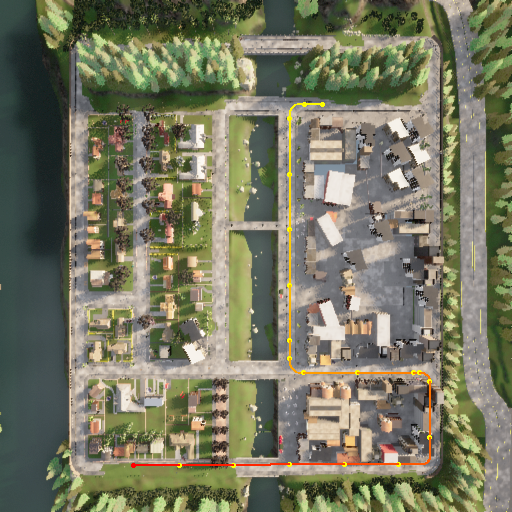
Figure 7: Town01 environment of the agent, with one of the routes used to collect data by the expert. The highlighted path has 740 meters, 20 points in the sparse trajectory (shown as yellow dots) and 762 points in the dense point trajectory (not shown).

V-B Training

The training was conducted using six parallel actors in a synchronous manner, with each actor running its own instance of the CARLA simulator. In the simulation, each episode begins with the vehicle at zero speed at a random starting point. The episode concludes upon the occurrence of any infraction, collision, or lane invasion, and a new episode begins with the vehicle located at a random point of the map to provide diversified experiences for each policy update.

At every $12,288$ environment interactions (steps), the agent’s architecture is updated in a central computer: the parametrized policy using loss function (7) is trained for 20 epochs using PPO (K=20), while the GAIL’s Discriminator is trained for 2 epochs (J=2) on these $12,288$ samples; and the CGAN’s Generator for BEV with the loss function (1) is trained for 4 epochs, while its Discriminator for 4 epochs. This process corresponds to one training cycle of the full hGAIL. A new cycle will collect the next $12,288$ samples from all the actors, and execute the training as described above again. As six parallel actors are used, 2,048 steps or environment interactions per actor are recorded, totalling the 12,288 environment interactions. Thus, the episode does not have to end for a policy update to happen. It is important to note that at any given moment, any of the six actors may be interacting with the environment in different parts of the environment. Additional hyperparameters’s values can be found in Tables  I and Table II for the GAIL and GAN parts of hGAIL, respectively.

It is worth noting that the GAN’s generator of hGAIL is pretrained on the fixed set of the ten expert trajectories (with 21,287 pairs of input and BEV targets) for 4 epochs in a supervised way. After this pretraining, the batch of the real BEV samples for training the GAN’s discriminator evolves with the agent’s training and corresponds exactly to the batch of $12,288$ samples collected by the six parallel actors. The simulator automatically labels them with the real BEV desired output as it is able to compute the topdown view of the vehicle. This happens at every $12,288$ steps executed by all actors together and, thus, the training of the GAN for generating a mid-level input representation is accomplished as the agent interacts with the environment, similarly to a strategy for decoupling representation learning from reinforcement learning in [41]. The idea is that, once the GAN’s training is turned off, the predicted BEV from the GAN’s generator could be used in a real setting where the BEV computation is not available. The detailed algorithm for hGAIL training is shown in algorithm $(\ref{alg:hgail})$.

TABLE I: Hyperparameters for GAIL

Description	Value
Parallel environments ($N$)	$6$
Initial adam step size (lr)	$2.0\times 10^{-5}$
Adam step size exponential decay ($\lambda_{lr}$)	$0.96$
Number of PPO epochs (K)	$20$
Mini-batch size (m)	$256$
Discount ($\gamma$)	$0.99$
GAE parameter ($\lambda$)	$0.9$
Clipping parameter ($\epsilon$)	$0.2$
Value Function clipping parameter ($\epsilon_{vf}$)	$0.2$
Value Function coefficient ($c_{1}$)	$0.5$
Entropy coefficient ($c_{2}$)	$0.01$
Exploration coefficient ($c_{3}$)	$0.05$
Timesteps per epoch (T)	$12288$
GAIL gamma ($\gamma_{gail}$)	$0.004$
GAIL gamma decay ($\lambda_{gail}$)	$1.0$
Discriminator adam step size (lr)	$2.5\times 10^{-4}$
Number discriminator epochs (J)	$2$

TABLE II: Hyperparameters for CGAN

Description	Value
Adam step size (lr)	$2.0\times 10^{-4}$
Number of GAN epochs (K)	$4$
Mini-batch size (m)	$32$
Patch size ($\gamma$)	$(10,10)$
Resize ($\lambda$)	$(192,192)$
Lambda pixel ($\epsilon$)	$100$

Input: Expert transitions buffer $\mathcal{B}_{E}$;

Input parameters: Policy Actor: $\theta$, Critic: $\phi$, Discriminator: $\omega$ ;

Pretrain CGAN using samples from $\mathcal{B}_{E}$;

for $episode=1,2,\dots$ do

       // Collect trajectory samples from the environment

       for $t=1,2,\dots,T$ do

             // $x_{t}$ are CGAN $G(.)$’s inputs; $y_{t}$ is the true BEV

             Choose action $a_{t}\sim\pi_{\theta}\left(G\left(x_{t}\right)\right)$; $v_{t}\leftarrow V_{\phi}\left(G\left(x_{t}\right)\right)$;

             $x_{t+1},y_{t+1}\leftarrow act(a_{t})$;

             Add $\left(x_{t},y_{t},G\left(x_{t}\right),a_{t},v_{t}\right)$ to the buffer $\mathcal{B}_{\pi}$;

            

       end for

      for $j=1,2,\dots,J$ do /* Update GAIL’s discriminator */

             Sample $\{(y^{(i)},a^{(i)})^{\pi}\}^{m}_{i=1}$ and $\{(y^{(i)},a^{(i)})^{E}\}^{m}_{i=1}$ from policy transitions buffer $\mathcal{B}_{\pi}$ and expert transitions $\mathcal{B}_{E}$;

             Update the policy discriminator parameters $w$ to increase $(\ref{eq:wgail2})$;

            

       end for

      Compute advantage $A_{t\in\{1,2,\dots,T\}}$ based on advantage function $A_{\omega,\phi}$ $(\ref{eq:advantage})$ and add to policy transitions buffer $\mathcal{B}_{\pi}$;

       for $k=1,2,\dots,K$ do /* Update agent using PPO */

             Sample $\left\{\left(G\left(x^{(i)}\right),a^{(i)},A^{(i)}\right)^{\pi}\right\}^{m}_{i=1}$ from policy transitions buffer $\mathcal{B}_{\pi}$;

             Update the policy generator parameters $\theta$ to optimize $(\ref{eq:bcgail_explo})$;

            

       end for

      Train CGAN using samples from $\mathcal{B}_{\pi}$;

      

end for

Algorithm 1 Hierarchical Generative Adversarial Imitation Learning

V-C Evaluation

The main evaluation environment is town02, shown in Fig. 8. It was used to test how well the hGAIL agent can generalize its driving skills to unseen, new environments. All experiments below consider agents trained exclusively in town01 environment.

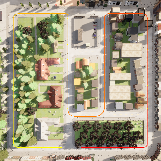
Figure 8: Town02 environment of the agent, with one of the routes used to evaluate the agent trained in town02. The highlighted path has 1010 meters, 29 points in the sparse trajectory (shown as yellow dots) and 1030 points in the dense point trajectory (not shown).

The training progress can be seen in Fig. 9 for hGAIL, GAIL w/ real BEV, and GAIL from cameras agents. The second agent is trained directly on the real birds-eye view image computed from the simulator, while the last one is trained with input coming directly from the three frontal cameras and sparse trajectory, disregarding any birds-eye view representation. The plot shows the average and standard deviation of the number of infractions for three runs for each agent’s stochastic policy.

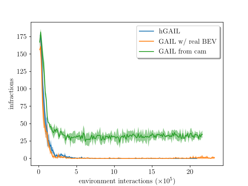
(a) With visual trajectory input

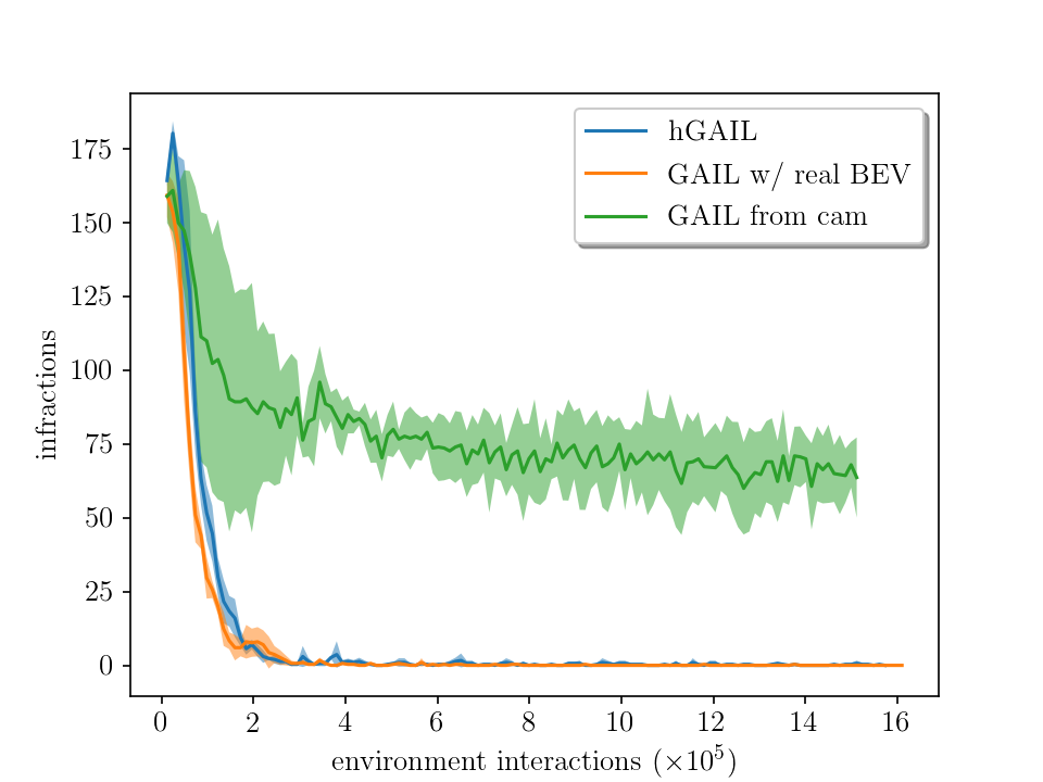
(b) Without visual trajectory input

Figure 9: Number of committed infractions vs. environment interactions during training in town1 environment. The top (bottom) plot shows the results for the agents receiving (disregarding) the sparse trajectory as visual input (trajectory 1x192x192 in Fig.5) in the corresponding CNN. For each method (hGAIL, GAIL with real Bird’s Eye View, GAIL from cameras), the average performance of three runs is depicted considering a stochastic policy. The shaded area represents the standard deviation. The GAIL from cameras agent fail to learn the task and keep the sum of committed infractions above zero, while the minimum of zero infractions is achieved by both hGAIL and GAIL with real BEV.

The resulting deterministic policies of each agent trained in town1 for all three runs are also evaluated in town2 as training evolves, as shown in Fig. 10. It shows the average percentage of completed routes from a total of six Leaderboard routes in town2 as learning proceeds. Each run uses a different agent trained exclusively in town1. Both hGAIL and GAIL with real BEV are able to generalize the learning in town1 to town2. Besides, the ablation on hGAIL agent of the visual input of the sparse trajectory negatively affect the evaluation performance. In this context, it is worth noticing that if we would have pretrained its GAN network for more epochs on the expert dataset, we would improve the performance of the hGAIL ablated (results not shown). This means that the sparse trajectory given as extra visual stimuli makes the GAN train faster.

In addition to the above three agents, other two agents were tested: the Behavior Cloning (BC) and GAIL from cameras agents. The BC agent consists of basically substituting the GAIL policy for a BC policy, which receives the BEV prediction from a GAN. Both BC and its associated GAN were trained on the same set of ten demonstration trajectories in an offline manner. Both of these agents are not shown in the plot, since they fail to learn to complete any route (staying at 0% if shown in Fig. 10).

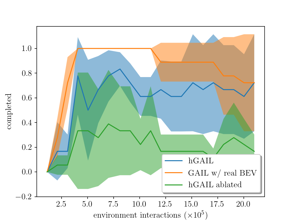
(a) Evaluation

Figure 10: Evaluation of agents in town2, trained exclusively in town1. The plot shows the percentage of completed routes from a total of six Leaderboard routes in town2 vs. environment interactions, averaged over three different runs, where each run entails a different agent trained only in town1. For each method (hGAIL, GAIL with real Bird’s Eye View, hGAIL ablated), the average performance of three runs is depicted considering a deterministic policy. The shaded area represents the standard deviation. Not shown in the plot, Behavior Cloning (BC) and GAIL from cameras agents fail to learn the task and complete any route (staying at 0% if shown in the plot). Both hGAIL and GAIL with real BEV are able to generalize the learning in town1 to town2. The hGAIL ablated agent receives no visual input of the sparse trajectory, but only its numeric vector.

After training, the agent was also evaluated at a given T intersection and compared to the target given by the expert. Fig. 11 shows the resulting trajectories, with blue and orange denoting the agent’s and expert’s trajectories, respectively. It is worth noting that the policy’s network in the hGAIL agent receives as input only the generated (fake) BEV mid-level image, the current speed, and last applied actions for throttle and steering. For instance, this BEV image corresponds to the topdown image with three channels from Fig. 3. It is important to observe that the only information denoting the desired movement for the agent comes from the yellow desired route in the drivable red area. This yellow route occupies the whole lane in the BEV image, which leaves open how the agent will learn to turn at certain intersections. In other words, the agent’s policy can not see directly the points in the sparse trajectory, as these points are fed to the GAN part of the architecture and not to the policy. This means that how we terminate the episode, such as through infractions and lane invasion, will influence to a great extent the type of behavior the agent learns. Such an example can be seen in the turns of Fig. 11, where the agent’s trajectory does not match exactly with the expert’s one. We conjecture that the behavior of the agent could have been made more similar to the expert if: the network of the agent’s policy would have received all the information that the expert receives as input (e.g., dense trajectory); the infractions would have been more strict; additional reward terms would have been added in the reward function to punish certain behaviors.

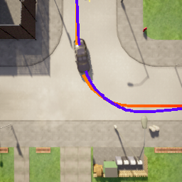
(a) top-right

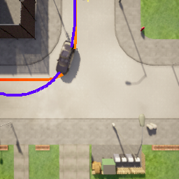
(b) top-left

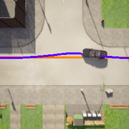
(c) right-left

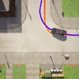
(d) right-top

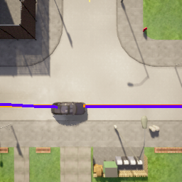
(e) left-right

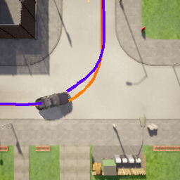
(f) left-top

Figure 11: Agent’s trajectories in town2 in blue color generated by the deterministic policy after training in town1 (at epoch 100) superimposed on the expert trajectory in orange color. At the same T intersection, 6 possible movements are possible: from top to right, top to left, right to left, right to top, left to right and left to top.

The agent trained only on town1 was also evaluated at every T intersection in town2 environment, i.e., 8 different T intersections, and compared to Behavior Cloning and GAIL from cameras agents. The latter corresponds to a GAIL agent with input directly from the vehicle’s three frontal cameras instead of the mid-level BEV input. The results are summarized in Table III, whose lines presents the results for each possible turn out of 6 in total at a given T intersection (as shown in Fig. 11). Thus, each turn, covering around 100 meters, was evaluated in 8 different T intersections, totalling 48 experiments for each agent. The success percentage for each turn type is given in this table, where we can see that hGAIL can turn without failing in all intersections and for all turn types except for one top-right intersection, while BC fails 50% of the times, and GAIL from cameras fails to learn most of the required driving behavior, succeeding only in 4 turns out of 48. This ablation of the GAN from hGAIL (which is the GAIL from cameras) shows the need for learning the mid-level input representation to succeed in this complex task. Additionally, notice that only hGAIL can finish complete trajectories (of around 1 km, as shown in Fig. 10), as both BC and GAIL from cameras fail in at least one turn type.

TABLE III: Evaluation performance for 8 T Intersections and 6 type of turns in Town2

Turn type	BC	hGAIL	GAIL from cam.	hGAIL ablated
Top-right	$0\%$	$88\%$	$0\%$	$100\%$
Top-left	$75\%$	$100\%$	$0\%$	$75\%$
Right-left	$50\%$	$100\%$	$25\%$	$100\%$
Right-top	$88\%$	$100\%$	$13\%$	$63\%$
Left-right	$88\%$	$100\%$	$13\%$	$100\%$
Left-top	$0\%$	$100\%$	$0\%$	$88\%$
All types	$50\%(24)$	$98\%(47)$	$8\%(4)$	$88\%(42)$

The evolution of training for the hGAIL agent in town1 can also be seen in Fig. 12, where the whole trajectory throughout the city is plot at three different moments in training. Early in the training process, the infractions or errors, given by red triangles, are frequent. These infractions decrease as learning proceeds.

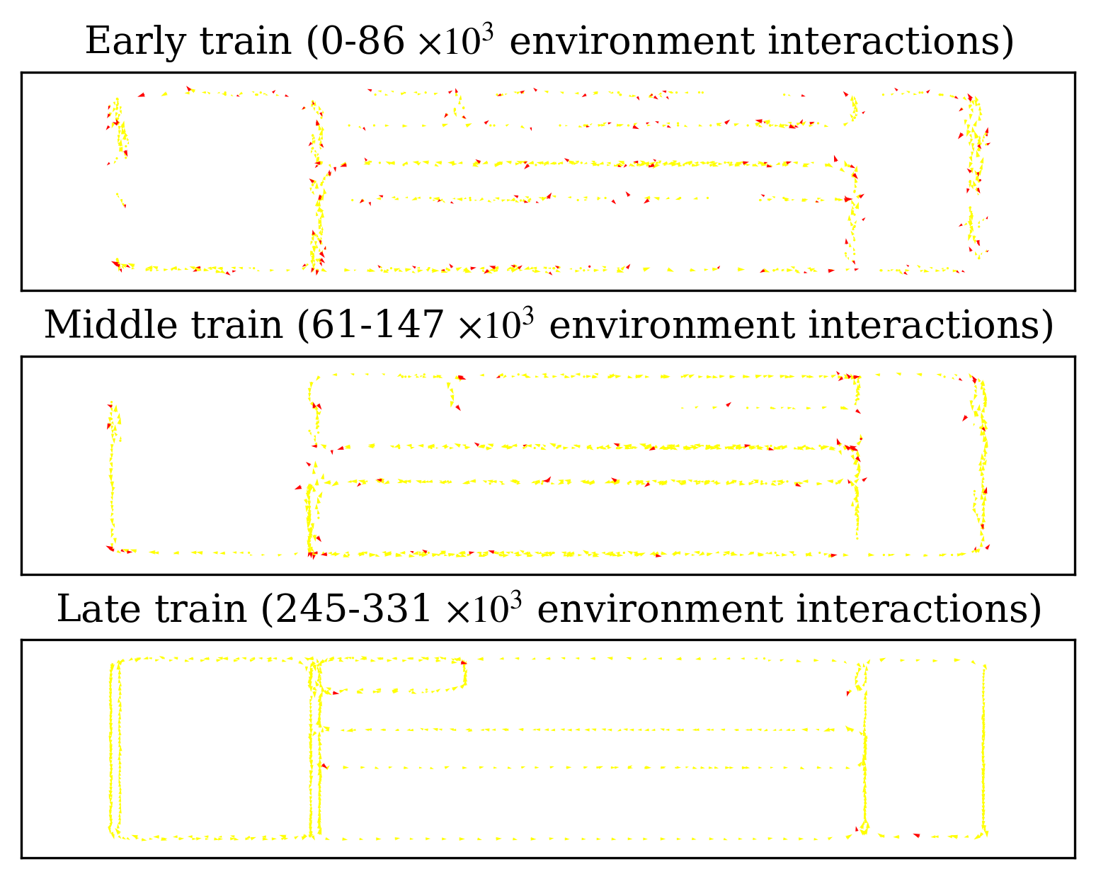
Figure 12: The vehicle’s trajectory, in yellow, during different moments of the training process. In the early training iterations, errors, marked in red color, are common. As training proceeds, less and less mistakes happen.

V-D Mid-level representation learning

Here, we present some results of the Birds’ Eye-View representation learned by the GAN’s generator of the hGAIL agent’s architecture. While this GAN learns in town01, Fig. 13 shows the evolution of the representations of five different vehicle’s positions taken in town02 at different training epochs of the agent in town1, where each row corresponds to a different particular position of the vehicle in the town02 environment. The first four columns are the input to the GAN’s generator, consisting of the images from the three frontal cameras and the sparse trajectory given as an image. The fifth column corresponds to the targets (labels), i.e., the BEV generated by the simulator, which is used to train the GAN’s generator. The other columns show the mid-level BEV representation evolving from a poor prediction at cycle 1 (after 12,288 environment steps) to a good enough prediction at cycle 32. It is worth noticing that the GAN has never seen town02, and was trained only on town01.

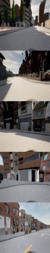
(a) left

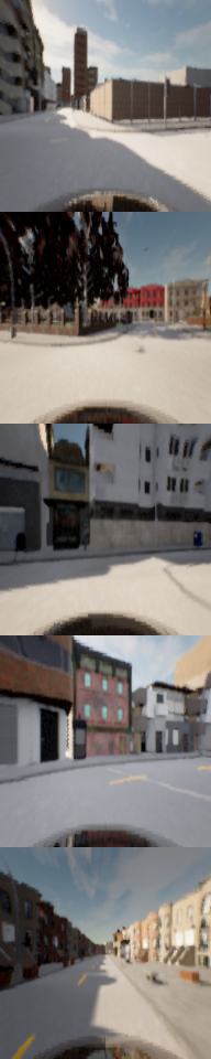
(b) cent.

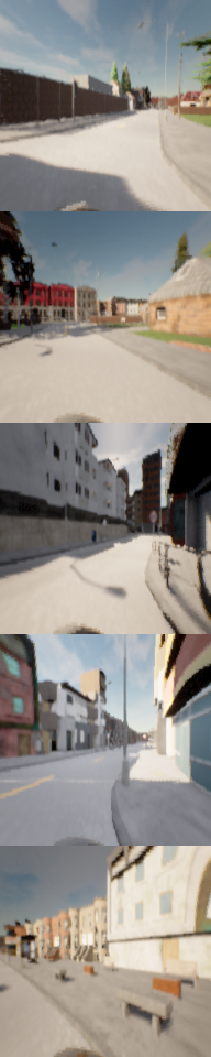
(c) right

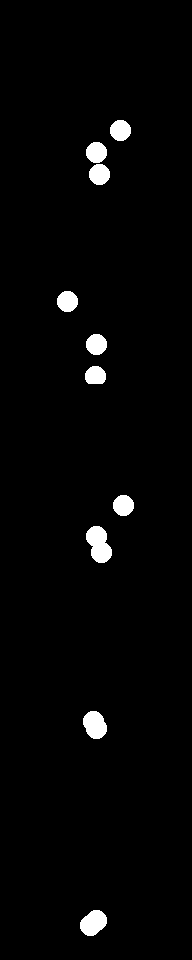
(d) traj.

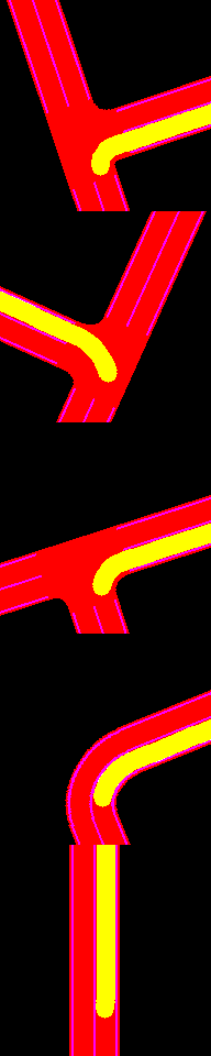
(e) target

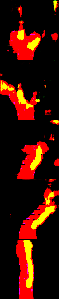
(f) 1 cy.

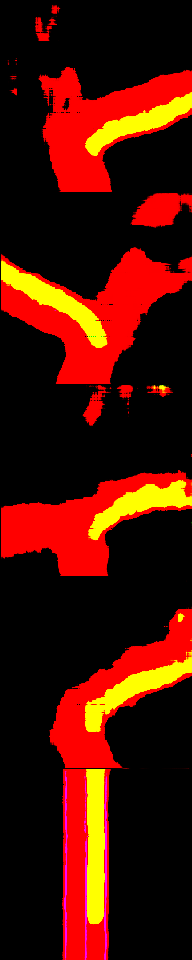
(g) 16 cy.

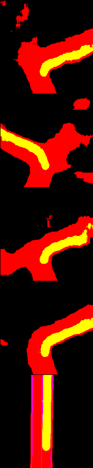
(h) 32 cy.

Figure 13: BEV generation as the agent goes through training. The first three colmns shows the images from the cemeras attached to the front of the vehicle. The fourth column show the plot from the point from the route planner The fifth column shows five BEV images computed by the simulator and are considered the target output. The following columns show the BEV images generated by the GAN from the agent’s architecture as it undergoes training, at: 12,288 environment steps (1 cycle), 208,896 environment steps (16 cycles), and 405,504 environment steps (32 cycles). One cycle is similar to the concept of epoch, and consists of the full training of hGAIL using the last 12,288 steps collected; however, each individual network of hGAIL is trained for different number of epochs in one training cycle (see Section V-B).

VI Conclusion

In this work, the hGAIL architecture was proposed to solve the autonomous navigation of a vehicle in an end-to-end approach, connecting sensory perceptions to low-level actions directly with neural networks (sensory-motor coupling), while learning mid-level input representations of the agent’s environment. hGAIL is an hierarchical Adversarial Imitation Learning architecture composed of two main modules: the CGAN which generates the Bird’s-Eye View (BEV) representation from the three frontal cameras of the vehicle, desired trajectory and high-level command, which is a mid-level (more abstract) input representation of the scene in front of the vehicle; and the GAIL which learns to control the vehicle based mainly on the BEV predictions from the CGAN as input.

Both GAIL and CGAN in hGAIL learns simultaneously in an adversarial way to control the agent and generate the input representations, respectively. The learning takes place in an urban city without pedestrians or other cars, but with dynamic routes that can change the path on the fly. Our experiments have shown that the mid-level input generated by CGAN is essential for the learning task as the GAIL exclusively from cameras (without BEV) fails to even learn the task, keeping a high-infraction rate through training. The BC agent with its associated GAN can complete some turns in the trajectories, but not consistently as hGAIL can. In fact, hGAIL, after training exclusively on ten expert trajectories from one city, was able to generalize its navigation skills to a new, unseen city, and complete 98% of all 48 possible turns in the eight T intersections from that new city.

This work has demonstrated the usefulness of mid-level BEV input for realistic navigation scenarios, but also that this input representation can be learned concomitantly with the agent’s policy training. Thus, the BEV generation is learned with the same data distribution used to train the agent’s policy, i.e., the expert dataset and the data generated by the agent. In future work, we are interested in: adding dynamic obstacles such as pedestrians and other vehicles, as well as traffic lights and other weather conditions; testing the generalization of the policy to other new cities; and sim2real experiments.

Gustavo Claudio Karl Couto graduated from the Militar Institute of Engineering in 2018 with a degree in Electronic Engineering. He is currently pursuing a master’s degree in automation and systems engineering at Federal University of Santa Catarina. His main areas of interest are robotics and intelligent systems. His current research focuses on applications of imitation learning algorithms in autonomous driving systems.

Eric Aislan Antonelo received the M.Sc. degree in computer engineering from Halmstad University, Halmstad, Sweden, in 2006, and the Ph.D. degree in computer engineering from Ghent University, Ghent, Belgium, in 2011. He is currently a Faculty Member with the Department of Automation and Systems Engineering, Federal University of Santa Catarina, Florianópolis, Brazil. His research is mainly focused on reservoir computing and machine learning for industrial applications (modeling, detection, and control tasks), as well as imitation learning approaches for autonomous vehicles.

References

- [1] M. Montemerlo, J. Becker, S. Bhat, H. Dahlkamp, D. Dolgov, S. Ettinger, D. Haehnel, T. Hilden, G. Hoffmann, B. Huhnke, D. Johnston, S. Klumpp, D. Langer, A. Levandowski, J. Levinson, J. Marcil, D. Orenstein, J. Paefgen, I. Penny, and S. Thrun, “Junior: The stanford entry in the urban challenge,” Journal of Field Robotics, vol. 25, pp. 569 – 597, 09 2008.
- [2] C. Urmson, J. Anhalt, D. Bagnell, C. Baker, R. Bittner, M. Clark, J. Dolan, D. Duggins, T. Galatali, C. Geyer, M. Gittleman, S. Harbaugh, M. Hebert, T. Howard, S. Kolski, A. Kelly, M. Likhachev, M. Mcnaughton, N. Miller, and D. Ferguson, “Autonomous driving in urban environments: Boss and the urban challenge,” Journal of Field Robotics, vol. 25, pp. 425–466, 01 2008.
- [3] B. Paden, M. Cáp, S. Z. Yong, D. S. Yershov, and E. Frazzoli, “A survey of motion planning and control techniques for self-driving urban vehicles,” IEEE Transactions on Intelligent Vehicles, vol. 1, pp. 33–55, 2016.
- [4] L. M. S. Parizotto and E. A. Antonelo, “Cone detection with convolutional neural networks for an autonomous formula student race car,” in 26th ABCM International Congress of Mechanical Engineering (COBEM 2021), 2021.
- [5] M. Bojarski, D. Del Testa, D. Dworakowski, B. Firner, B. Flepp, P. Goyal, L. D. Jackel, M. Monfort, U. Muller, J. Zhang, X. Zhang, J. Zhao, and K. Zieba, “End to end learning for self-driving cars,” 2016. [Online]. Available: https://arxiv.org/abs/1604.07316
- [6] H. Xu, Y. Gao, F. Yu, and T. Darrell, “End-to-end learning of driving models from large-scale video datasets,” 2016. [Online]. Available: https://arxiv.org/abs/1612.01079
- [7] M. Bansal, A. Krizhevsky, and A. Ogale, “Chauffeurnet: Learning to drive by imitating the best and synthesizing the worst,” 2018. [Online]. Available: https://arxiv.org/abs/1812.03079
- [8] F. Codevilla, M. Müller, A. López, V. Koltun, and A. Dosovitskiy, “End-to-end driving via conditional imitation learning,” 2018.
- [9] F. Codevilla, E. Santana, A. M. López, and A. Gaidon, “Exploring the limitations of behavior cloning for autonomous driving,” 2019.
- [10] S. Ross and D. Bagnell, “Efficient reductions for imitation learning.” Journal of Machine Learning Research - Proceedings Track, vol. 9, pp. 661–668, 01 2010.
- [11] A. Prakash, A. Behl, E. Ohn-Bar, K. Chitta, and A. Geiger, “Exploring data aggregation in policy learning for vision-based urban autonomous driving,” in 2020 IEEE/CVF Conference on Computer Vision and Pattern Recognition (CVPR), 2020, pp. 11 760–11 770.
- [12] S. Ross, G. Gordon, and D. Bagnell, “A reduction of imitation learning and structured prediction to no-regret online learning,” in Proceedings of the Fourteenth International Conference on Artificial Intelligence and Statistics, ser. Proceedings of Machine Learning Research, G. Gordon, D. Dunson, and M. Dudík, Eds., vol. 15. Fort Lauderdale, FL, USA: PMLR, 11–13 Apr 2011, pp. 627–635. [Online]. Available: https://proceedings.mlr.press/v15/ross11a.html
- [13] A. Y. Ng, S. J. Russell et al., “Algorithms for inverse reinforcement learning.” in ICML, 2000, pp. 663–670.
- [14] J. Ho and S. Ermon, “Generative adversarial imitation learning,” in Advances in Neural Information Processing Systems, 2016, pp. 4565–4573.
- [15] G. C. Karl Couto and E. A. Antonelo, “Generative adversarial imitation learning for end-to-end autonomous driving on urban environments,” in 2021 IEEE Symposium Series on Computational Intelligence (SSCI), 2021, pp. 1–7.
- [16] Z. Zhang, A. Liniger, D. Dai, F. Yu, and L. Van Gool, “End-to-end urban driving by imitating a reinforcement learning coach,” in 2021 IEEE/CVF International Conference on Computer Vision (ICCV), 2021, pp. 15 202–15 212.
- [17] A. Sax, J. O. Zhang, B. Emi, A. Zamir, S. Savarese, L. Guibas, and J. Malik, “Learning to navigate using mid-level visual priors,” arXiv preprint arXiv:1912.11121, 2019.
- [18] M. Müller, A. Dosovitskiy, B. Ghanem, and V. Koltun, “Driving policy transfer via modularity and abstraction,” arXiv preprint arXiv:1804.09364, 2018.
- [19] A. Mousavian, A. Toshev, M. Fišer, J. Košecká, A. Wahid, and J. Davidson, “Visual representations for semantic target driven navigation,” in 2019 International Conference on Robotics and Automation (ICRA). IEEE, 2019, pp. 8846–8852.
- [20] W. Yang, X. Wang, A. Farhadi, A. Gupta, and R. Mottaghi, “Visual semantic navigation using scene priors,” arXiv preprint arXiv:1810.06543, 2018.
- [21] P. Isola, J.-Y. Zhu, T. Zhou, and A. A. Efros, “Image-to-image translation with conditional adversarial networks,” in 2017 IEEE Conference on Computer Vision and Pattern Recognition (CVPR), 2017, pp. 5967–5976.
- [22] R. Jena, C. Liu, and K. Sycara, “Augmenting gail with bc for sample efficient imitation learning,” arXiv preprint arXiv:2001.07798, 2020.
- [23] P. Cai, S. Wang, Y. Sun, and M. Liu, “Probabilistic end-to-end vehicle navigation in complex dynamic environments with multimodal sensor fusion,” IEEE Robotics and Automation Letters, vol. 5, no. 3, pp. 4218–4224, 2020.
- [24] P. Cai, H. Wang, H. Huang, Y. Liu, and M. Liu, “Vision-based autonomous car racing using deep imitative reinforcement learning,” IEEE Robotics and Automation Letters, vol. 6, no. 4, pp. 7262–7269, 2021.
- [25] A. Kuefler, J. Morton, T. Wheeler, and M. Kochenderfer, “Imitating driver behavior with generative adversarial networks,” in Intelligent Vehicles Symposium (IV), 2017 IEEE. IEEE, 2017, pp. 204–211.
- [26] E. Bronstein, M. Palatucci, D. Notz, B. White, A. Kuefler, Y. Lu, S. Paul, P. Nikdel, P. Mougin, H. Chen et al., “Hierarchical model-based imitation learning for planning in autonomous driving,” arXiv preprint arXiv:2210.09539, 2022.
- [27] K. He, X. Zhang, S. Ren, and J. Sun, “Deep residual learning for image recognition,” in 2016 IEEE Conference on Computer Vision and Pattern Recognition (CVPR), 2016, pp. 770–778.
- [28] K. Ota, D. K. Jha, and A. Kanezaki, “Training larger networks for deep reinforcement learning,” arXiv preprint arXiv:2102.07920, 2021.
- [29] Y. Wang, D. Zhang, J. Wang, Z. Chen, Y. Li, Y. Wang, and R. Xiong, “Imitation learning of hierarchical driving model: From continuous intention to continuous trajectory,” IEEE Robotics and Automation Letters, vol. 6, no. 2, pp. 2477–2484, 2021.
- [30] S. Teng, L. Chen, Y. Ai, Y. Zhou, Z. Xuanyuan, and X. Hu, “Hierarchical interpretable imitation learning for end-to-end autonomous driving,” IEEE Transactions on Intelligent Vehicles, vol. 8, no. 1, pp. 673–683, 2023.
- [31] M. Bloem and N. Bambos, “Infinite time horizon maximum causal entropy inverse reinforcement learning,” in Decision and Control (CDC), 2014 IEEE 53rd Annual Conference on. IEEE, 2014, pp. 4911–4916.
- [32] I. Goodfellow, J. Pouget-Abadie, M. Mirza, B. Xu, D. Warde-Farley, S. Ozair, A. Courville, and Y. Bengio, “Generative adversarial nets,” in Advances in neural information processing systems, 2014, pp. 2672–2680.
- [33] D. P. Kingma and J. Ba, “Adam: A method for stochastic optimization,” arXiv preprint arXiv:1412.6980, 2014.
- [34] J. Schulman, F. Wolski, P. Dhariwal, A. Radford, and O. Klimov, “Proximal policy optimization algorithms,” CoRR, vol. abs/1707.06347, 2017. [Online]. Available: http://arxiv.org/abs/1707.06347
- [35] M. Zhang, Y. Wang, X. Ma, L. Xia, J. Yang, Z. Li, and X. Li, “Wasserstein distance guided adversarial imitation learning with reward shape exploration,” 2020 IEEE 9th Data Driven Control and Learning Systems Conference (DDCLS), Nov 2020. [Online]. Available: http://dx.doi.org/10.1109/DDCLS49620.2020.9275169
- [36] I. Gulrajani, F. Ahmed, M. Arjovsky, V. Dumoulin, and A. Courville, “Improved training of wasserstein gans,” 2017.
- [37] Y. Li, J. Song, and S. Ermon, “Infogail: Interpretable imitation learning from visual demonstrations,” 2017.
- [38] O. Ronneberger, P. Fischer, and T. Brox, “U-net: Convolutional networks for biomedical image segmentation,” in International Conference on Medical image computing and computer-assisted intervention. Springer, 2015, pp. 234–241.
- [39] I. G. Petrazzini and E. A. Antonelo, “Proximal policy optimization with continuous bounded action space via the beta distribution,” in 2021 IEEE Symposium Series on Computational Intelligence (SSCI). IEEE, 2021, pp. 1–8.
- [40] D. Chen, B. Zhou, V. Koltun, and P. Krähenbühl, “Learning by cheating,” 2019.
- [41] A. Stooke, K. Lee, P. Abbeel, and M. Laskin, “Decoupling representation learning from reinforcement learning,” in International Conference on Machine Learning. PMLR, 2021, pp. 9870–9879.