Symbolic Metamodels for Interpreting Black-boxes Using Primitive Functions

Abstract

One approach for interpreting black-box machine learning models is to find a global approximation of the model using simple interpretable functions, which is called a metamodel (a model of the model). Approximating the black-box with a metamodel can be used to 1) estimate instance-wise feature importance; 2) understand the functional form of the model; 3) analyze feature interactions. In this work, we propose a new method for finding interpretable metamodels. Our approach utilizes Kolmogorov superposition theorem, which expresses multivariate functions as a composition of univariate functions (our primitive parameterized functions). This composition can be represented in the form of a tree. Inspired by symbolic regression, we use a modified form of genetic programming to search over different tree configurations. Gradient descent (GD) is used to optimize the parameters of a given configuration. Our method is a novel memetic algorithm that uses GD not only for training numerical constants but also for the training of building blocks. Using several experiments, we show that our method outperforms recent metamodeling approaches suggested for interpreting black-boxes.

1 Introduction

In the recent years machine learning (ML) algorithms made several breakthroughs in issuing accurate predictions. There is however a growing need to improve trustworthiness of these models. Providing accurate predictions is not enough in high-stake applications like healthcare where an agent (e.g. clinician) needs to interact with the model. In these applications the agent usually needs to understand how a particular prediction is issued. Especially, if the model prediction (say treatment plan) is different from what the clinician has in mind, explaining the model is vital. Complicated ML models like neural networks are essentially black-boxes to humans, and that is why interpretability methods are important and have gained significant attention in recent years (Ribeiro, Singh, and Guestrin 2016b; Lundberg and Lee 2017; Guidotti et al. 2018; Arnaldo, Krawiec, and O’Reilly 2014; Zhang, Solar-Lezama, and Singh 2018; Alvarez-Melis and Jaakkola 2018; Arrieta et al. 2020; Lou et al. 2013; Doshi-Velez and Kim 2017).

There exist two key approaches to bring interpretability to machine learning models: (1) by designing inherently interpretable models (Rudin 2019; Chen et al. 2019; Alvarez-Melis and Jaakkola 2018); or (2) by designing post-hoc methods to understand a pre-trained model (Ribeiro, Singh, and Guestrin 2016a; Lipton 2016). In this work, we focus on the second approach that includes methods to analyze a trained model locally and globally (Montavon, Samek, and Müller 2018). The local interpretability methods focus on instance-wise explanations, which although useful, provide little understanding of a model’s global behaviour (Ribeiro, Singh, and Guestrin 2016b; Lundberg and Lee 2017). Hence, researchers have proposed multiple techniques to interpret how a ML model behaves for a group of the instances. Some examples of global analysis methods include permutation feature importance (Molnar 2019), activation-maximization (Erhan et al. 2009), and learning globally surrogate models (Thrun 1995; Craven and Shavlik 1996).

Our work relates to the last approach that aims to learn interpretable proxies by approximating the behaviour of black-box ML models for multiple instances. Some efforts in this category include methods to approximate neural networks with if-then rules (Thrun 1995) or decision trees (Craven and Shavlik 1996) and the method to approximate matrix factorisation models using Bayesian networks and simple logic rules (Carmona et al. 2015). Our work is mostly relevant to a different category of approaches for learning interpretable proxies that focuses on approximating black-box functions with symbolic metamodels. A proper interpretable metamodel can enjoy benefits of different categories of interpretability methods. For example, a metamodel may provide insight into the interactions of different features and how they contribute in producing results. The metamodel can be locally approximated (e.g. using Taylor series) to generate instance-wise explanations. Moreover, it may be used for scientific discovery by revealing underlying laws governing the observed data (Schmidt and Lipson 2009; Wang, Wagner, and Rondinelli 2019; Udrescu and Tegmark 2020b).

Symbolic regression (SR) (Koza 1994), has been the primary approach for finding approximate metamodels. In SR, there exist some fixed mathematical building blocks (e.g. summation operation), and the Genetic Programming (GP) algorithm searches over possible expressions that can be composed by combining the building blocks. We will explain SR in more details in Section 2 and compare it with our proposed method in Section 4. The major limitation of SR is that it uses a set of limited predefined building blocks and the search spaces grows when the number of building blocks increase. Two recent papers, which are the most relevant to our work (Alaa and van der Schaar 2019; Crabbe et al. 2020), address this issue by suggesting the use of a parametric trainable class of functions instead of fixed building blocks. In particular, they suggest using Meijer G-functions (we briefly introduce this class in Section 2). Note that these are univariate functions, in order to use them in multivariate settings, (Alaa and van der Schaar 2019) considers a heuristic approximation of Kolmogorov superposition theorem (KST) and (Crabbe et al. 2020) considers the projection pursuit method (in Section 4, we show that their method can be also considered as an approximation of KST). Both these works start from a general framework, however, they make some restricting assumptions that limit the usability and coverage of their methods. For example, the simple function $x_{1}x_{2}$ (here $x_{i}$’s are features) cannot be represented with the method given in (Crabbe et al. 2020). Similarly, the method in (Alaa and van der Schaar 2019) fails to represent the product of three features $x_{1}x_{2}x_{3}$. Another limitation of the proposed approaches is that although most of familiar functions are indeed special cases of Meijer G-functions, for almost all parameters, Meijer G-functions do not have familiar closed form representation. Therefore, in practice, in the training of parameters it is very unlikely to obtain a set of parameters that are “interpretable”.

High level idea and contribution: In this work, we address the above challenges by proposing a new methodology to learn symbolic metamodels. Our approach is a generalization of (Alaa and van der Schaar 2019) and (Crabbe et al. 2020) as we consider a more general approximation of KST (see section 4). We represent the KST expression using trees where edges represent simple parameterized functions (e.g., exponential function). We use gradient descent to train parameters of these functions and employ GP to search for the tree that most accurately approximates the black-box function. We demonstrate the efficacy of our proposed method through several experiments. The results suggest that our approach for estimating symbolic metamodels is comparatively more generic, accurate, and efficient than other symbolic metamodeling methods. In this work we are using our proposed method to provide interpretations, however, this method can be considered in general as a new GP method. Our method should be classified as a memetic algorithm where a population based method is paired with a refinement method (in our case gradient descent) (Chen et al. 2011). To the best of our knowledge, this is the first method that uses gradient descent not only for training numerical constants but also for the training of building blocks, i.e., primitive functions.

2 Preliminaries

In this section, we present a brief overview of building blocks of our proposed method: genetic programming; and classes of trainable functions.
Genetic Programming and symbolic regression: Genetic programming (GP) is an optimization method inspired by law of natural selection proposed by Koza in 1994 (Koza 1994). It starts with a population of random programs for a particular task and then evolves the population in each iteration with operations inspired by natural genetic processes. The idea is that after enough iterations the population evolves and a fit program can be found in later generations. The two typical operations for evolving are crossover and mutation. In crossover, we choose the fittest programs (the fitness criterion is predefined for the task in hand) for reproduction of next generation (parents) and swap random parts of the selected pairs. In mutation operation, a random part of a program is substituted by some other randomly generated part of a program. One instance of using GP is for optimization in Symbolic Regression (SR), where the goal is to find a suitable mathematical expression to describe some observed data. In this setting, each program consists of primitive building blocks such as analytic functions, constants, and mathematical operations. The program is usually represented with a tree, where each node is representing one of the building blocks. We refer to (Orzechowski, La Cava, and Moore 2018; Wang, Wagner, and Rondinelli 2019) for more details on SR. GP as a population base optimization method can be paired with other refinement methods. For example, here we are using both GP and GD in our model. This type of methods are called memetic algorithms. In particular, our method should be classified as a Lamarckian memetic algorithm, where Lamarckian refers to the method of inheritance in GP search. we refer to (Emigdio et al. 2014; Chen et al. 2011) for more details on taxonomy of GP methods.

Class of trainable functions: In contrast with SR which uses fixed building blocks, our proposed approach (similar to (Alaa and van der Schaar 2019) and (Crabbe et al. 2020)) uses a class of trainable parameterized functions as building blocks. One such class of functions is called Meijer G-functions and have been used in two recent approaches to learn symbolic metamodels (Meijer 1946, 1936). A Meijer-G function $G^{m,n}_{p,q}$ is defined as an integral along the path $\mathcal{L}$ in the complex plane.

$$G^{m,n}_{p,q}\left({}^{a_{1},\ldots,a_{p}}_{b_{1},\ldots,b_{q}}\,\Big{|}\,x\right)=$$

$$\frac{1}{2\pi i}\int_{\mathcal{L}}\frac{\prod^{m}_{j=1}\Gamma(b_{j}-s)\prod^{n}_{j=1}\Gamma(1-a_{j}+s)}{\prod^{q}_{j=m+1}\Gamma(1-b_{j}+s)\prod^{p}_{j=n+1}\Gamma(a_{j}+s)}\,x^{s}\,ds,$$

where $0\leq m\leq q$ and $0\leq n\leq p$ are all integers, and $a_{i},b_{j}\in\mathbb{R}$ for $1\leq i\leq p$ and $1\leq j\leq q$. $\mathcal{L}$ is a path which separates poles of $\Gamma(1-b_{j}+s)$ from poles of $\Gamma(a_{j}+s)$. By fixing $m,n,p,q$ we have a class of parameterized functions ($a_{i}$’s and $b_{i}$’s are parameters), which can be trained using gradient descent. We refer to (Beals and Szmigielski 2013) for a more detailed definition of these functions. Meijer G-functions are rich set of functions that have most of the familiar functions which we think of as interpretable as special cases. For example,

However, when trained using gradient descent (GD), the final parameters for Meijer G-functions almost always will not have an interpretable closed form. This limits insight into the functional form of the black-box model. Hence, in this work, we propose using classes of simple, interpretable, parameterized functions that can be efficiently optimized using GD. The class of functions can be chosen by a domain expert for each particular task. We will discuss the selection of primitive functions further in Appendix C. Specifically, here we demonstrate our approach using the following five parameterized functions. In Appendix C, we show that our presented results will not significantly change with using other set of primitive functions.

$$f_{1}(a,b,c,d|x)=ax^{3}+bx^{2}+cx+d,\,f_{2}(a,b|x)=ae^{-bx}$$

$$f_{3}(a,b,c|x)=a\sin(bx+c),\,f_{4}(a,b,c|x)=a\log(bx+c),$$

$$f_{5}(a,b,c,d|x)=ax/(bx^{2}+cx+d).$$

Remark. It is important to revisit that our proposed framework is generic and can accommodate any trainable class of functions, including Meijer G.

3 Method

Assume that a black box function $f:\mathcal{X}\to\mathbb{R}$ is trained on a dataset. Our goal is to find an interpretable function $g$ which approximates $f$. To this end, we restrict $g$ to belong to the class of functions $\mathcal{G}$ which are deemed to be interpretable. Therefore, we want to find the solution to the following optimization problem:

$$\operatorname*{arg\,min}_{g\in\mathcal{G}}\ell(f,g),$$ (1)

where $\ell$ is our loss function of choice. In this work, we assume $\ell$ to be mean square loss

$$\ell(f,g)=\int_{\mathcal{X}}(g(x)-f(x))^{2}dx.$$ (2)

In order to approximate multivariate function $f$, we deploy Kolmogorov superposition theorem (Kolmogorov 1957) which states that any multivariate continuous function (with $d$ variables) has a representation in terms of univariate functions as follows:

$$g(\bm{x})=g(x_{1},\cdots,x_{d})=\sum_{i=1}^{2d+1}g^{out}_{i}\left(\sum_{j=1}^{d}g^{in}_{ij}(x_{j})\right).$$ (3)

In our setting, each of $g_{ij}^{in}$ and $g_{i}^{out}$ can be a function from $\mathcal{G}$. However, fully implementing this equation (especially, using computationally expensive Meijer G-functions) is impractical even for moderate values of $d$. Therefore, an approximation is proposed in (Alaa and van der Schaar 2019) by considering a single outer function which is set to be identity and adding multiplication of all pairs of attributes to capture their correlation (we discuss this method in more details in Section 4). In this work we propose another method for approximating Equation (3).

3.1 Approximating KST

In our method, we approximate KST using trees with $L<2d+1$ middle nodes, where each of them is connected to only a subset of inputs. We denote the middle nodes with $h_{i}$, for $1\leq i\leq L$. Our approximation can be represented via a three layered tree (see Figure 1). There is a single root node at the top of the tree which is connected to $L$ middle nodes. Each middle node is connected to a subset of bottom layer nodes. The bottom layer of the tree has $d$ nodes corresponding to $d$ features. For simplicity, when it is not confusing, we call the node corresponds to $i$th feature by $x_{i}$.

Note that each edge in the graph represents a univariate function. We denote the function corresponding to the edge between $h_{i}$ and the root with $g_{h_{i}}$ (these are the outer functions), and the function corresponding to an edge between $h_{i}$ and $x_{j}$ is denoted by $g_{ij}$ (inner functions). The argument of $g_{ij}$ is naturally the feature it is connected to, namely $x_{j}$, and the argument of $g_{h_{i}}$ is the summation of all incoming functions to $h_{i}$. That is, $\sum_{j\in\mathcal{N}(h_{i})}g_{ij}(x_{j}),$ where $\mathcal{N}(h_{i})$ denotes the neighbours of node $h_{i}$ in the graph. Finally, for the root node we sum all the outputs of all $L$ middle layer functions. Therefore, each tree is representing a function from $\mathcal{X}$ to $\mathbb{R}$, which can be expressed as follows:

$$g(\bm{x})=\sum_{i=1}^{L}g_{h_{i}}\left(\sum_{j\in\mathcal{N}(h_{i})}g_{ij}(x_{j})\right).$$ (4)

3.2 Using GP for Training of Metamodels

Now we want to solve the optimization problem in (1), where $\mathcal{G}$ is the set of all functions that can be represented in form of Equation (4), where all $g_{ij}$ and $g_{h_{i}}$ are drawn from the class of primitive parameterized functions. We propose solving this optimization problem by running a version of genetic programming algorithm. The tree representation of Equation (4), resembles the trees in symbolic regression that represents each program. Note that, unlike normal GP, here our constructed trees has a fixed structure of three layers, and also edges are representing functions. Hence we need to modify GP accordingly. In this section, we explain the details of our algorithm.

Figure 1: A sample tree structure, each edge is representing a univariate function

Producing random trees

In the first step, we produce $M$ random trees $T_{1},\cdots,T_{M}$. Each tree $T_{i}$ has $L_{i}$ middle nodes, where $L_{i}$ is an integer in $[l_{1},l_{2}]$. $l_{1}$ and $l_{2}$ are important hyperparameters, determining number of middle nodes. For each of $L_{i}$ middle nodes, a random subset of bottom layers will be chosen to be connected to this node. At first instance, for all $1\leq u\leq L_{i}$ and $1\leq v\leq d$, we connect $h_{u}$ and $x_{v}$ with probability $0<p_{0}$. Then if there exist an $x_{v}$ which is not connected to any of the middle nodes. We choose $1\leq u\leq L_{i}$ uniformly at random and then connect $x_{v}$ and $h_{u}$ to ensure every $x_{i}$ is connected to at least one of the middle nodes. $p_{0}$ is the parameter that controls sparsity of the produced graphs, which is one of the main factors that determine the complexity of the training procedure. Each edge is representing a function from our class of primitive functions, thus we uniformly at random choose one of the function classes for each edge and also initialize its parameters with samples from normal distribution.

Training phases

In the training phase, for each tree, we update the parameters of each edge using gradient descent. We choose a constant $k$ and apply $k$ gradient descent updates on the parameters of functions $g_{h_{i}}$ and $g_{ij}$. Let $g^{\prime}_{h_{i}}(x)=\frac{dg_{h_{i}}(x)}{dx}$. For $a$ one of the parameters of $g_{ij}$ and $b$ a parameter of $g_{h_{i}}$, the gradient of $g$ with respect to $a$ and $b$ can be computed as follows (recall that $g$ is representing the metamodel):

$$\frac{\partial g(\bm{x})}{\partial a}=\frac{\partial g_{ij}(x_{j})}{\partial a}\cdot g^{\prime}_{h_{i}}\left(\sum_{k\in\mathcal{N}(h_{i})}g_{ik}(x_{k})\right),$$ (5)

$$\frac{\partial g(\bm{x})}{\partial b}=\frac{\partial g_{h_{i}}}{\partial b}\left(\sum_{j\in\mathcal{N}(h_{i})}g_{ij}(x_{j})\right).$$ (6)

In this work, we choose a fixed learning rate and leave the exploration of using more advanced optimization techniques for future work (this is compatible with (Alaa and van der Schaar 2019) and (Crabbe et al. 2020), and allows us to have a fair comparison with these works).

Evaluation fitness of metamodels

For evaluating fitness of the trained metamodels, we uniformly at random sample $m$ points from $\mathcal{X}$ and query the output of black-box $f$ and metamodels $g_{1},\cdots,g_{M}$ on these $m$ points and compute the mean square loss for the metamodels to approximate (2) (the output of $f$ is considered as the ground truth). If any of the $M$ models has a loss less than a predefined threshold we terminate the algorithm. Otherwise, we choose the $s$ fittest metamodels and discard the rest. These $s$ survived metamodels are the parents that will populate the next generation of trees in the evolution process for the next round of the algorithm.

Regularization: We can modify the fitness criterion to favor simpler models. For encouraging sparsity of the tree, we can add a term to the MSE error for penalizing trees that have more edges. Denoting total number of edges with $E$, we use this criterion for evaluation fitness of the trees ($\lambda$ is a hyperparameter):

$$\text{Fitness of a given tree}=\text{MSE}+\lambda E.$$ (7)

Evolution phase

In the evolution phase, we create the next generation of metamodels using survived trees. Similar to conventional GP algorithm, here we also define two operations to perform on each tree: Crossover and Mutation. For each of the $s$ chosen trees like $T$, we first pass on $T$ to the next generation, then we randomly choose $\frac{M}{s}-1$ times one of the two operations, perform it on $T$, and add the resulting tree to the cohort of the next generation trees. Thus, the total number of trees in the next cohort is also $M$. Here we define the two operations which preserve the three layer structure of the trees:

• In the crossover operation, for $T$, we first randomly choose one of the nodes at the second layer of $T$. Then we uniformly at random choose one of the other $s-1$ trees, and then again uniformly at random choose one of its second layer nodes and replace that node alongside with all edges connected to that node with the chosen node in $T$. Notice that the edge connected to the root node will be also replaced. Moreover, note that the new tree will inherit the functions corresponding to replaced edges and their parameters.

• In the mutation operation, one of these two actions will be applied on the tree: 1) changing the function class of an edge, 2) removing an edge between the middle and input layers. In each round of mutation, we apply $n_{m}$ times one of these two actions on the tree. When we change the class of function for an edge, we also randomly reinitialize the parameters of the corresponding function.

The above two operations allow us to explore different configurations of trees and classes. A pseudo code of the algorithm and a flowchart is presented in Appendix A. We call our proposed method symbolic metamodeling using primitive functions (SMPF).

3.3 Different Types of Interpretation Using SMPF

Instance-wise feature importance: Similar to (Alaa and van der Schaar 2019) and (Crabbe et al. 2020) we can use the learned metamodel for estimating instance-wise feature importance. We can find the Taylor expansion of the metamodel around the data point of interest $\bm{x}_{0}$ and analyse its coefficients.

first order partial derivative with respect to $j$th feature can be computed using chain rule:

$$\frac{\partial g(\bm{x})}{\partial x_{j}}=\sum_{h_{i}\in\mathcal{N}(x_{j})}g^{\prime}_{h_{i}}\left(\sum_{j\in\mathcal{N}(h_{i})}g_{ij}(x_{j})\right)g^{\prime}_{ij}(x_{j}).$$ (9)

We will use this method in the instance-wise experiment. Importantly, we can also compute higher order coefficients for analyzing feature interactions.

Mathematical expressions: The final expression of the metamodel can provide insights into the functional form of the black-box function. For example, in the first experiment, we show that the metamodel correctly identifies that the black-box is an exponential function. Moreover, the inspection of mathematical expressions provides information about the interactions between the input features, and can potentially lead to understanding of previously unknown facts about the underlying mechanisms to domain experts. An idea for exploring in future work is inspecting the final cohort of graphs. For example, if in the last iteration, the average degree of a node is large across different graphs, this can show the importance of the corresponding feature. Similarly, when a subset of features are connected to a middle node it can show the interaction of those features.

4 Comparison with Related Works

In the experiments section, we compare our approach with three symbolic metamodeling methods. This section briefly introduces these approaches , highlighting their strengths and weaknesses. A table comparing our method with a wider range of methods is provided in the supplementary material.

Symbolic Metamodeling (SM) (Alaa and van der Schaar 2019): SM proposes using Meijer G-functions for interpreting black box models. In the derivation of their method, they also start with KST (3), however, with a different approximation: they consider only one outer function ($g^{out}$) and set that function to be identity (the inner functions are all Meijer G). This does not allow the features to interact, in order to fix this problem, they add multiplication of all pairs $x_{i}x_{j}$ to the features. This setting has two main issues, firstly this method cannot capture interaction of more than two features and does not show other forms of interactions apart from multiplication. Secondly, this approach introduces many new features which makes it impractical when $d$ increases. There are ${d\choose 2}+d$ features in total and there is a Meijer G-function corresponding to each of them which makes using SM computationally costly.

Symbolic Pursuit (SP) (Crabbe et al. 2020): SP is a subsequent work to SM and is designed to overcome some of its flaws. In particular, SP is designed to use fewer Meijer G-functions. The method is based on the Projection Pursuit algorithm in statistics (Friedman and Stuetzle 1981). In each step of the algorithm, a Meijer G-function will be fitted which minimizes the residual error between the metamodel and the black-box. The final metamodel will be the summation of all these Meijer G-functions. The input of each function is a linear combination of features. Thus, the final function will have the following formulation:

$$g(\bm{x})=\sum_{i=1}^{L}g_{i}\left(\sum_{j=1}^{d}c_{ij}x_{j}\right),$$ (10)

where $g_{i}$’s are Meijer G-functions. Importantly, the authors use a modified version of (10) where the arguments of Meijer G-functions are normalized such that they lie in the open interval of 0 to 1. Moreover, SP involves adding weights to the outer summation to allow mitigating the contributions of previously found functions, if needed.

Note that SP can be considered as one instance of our framework. The equation (10) is compatible with KST (3) and can be represented similar to Figure 1. In essence, all inner function (edges between bottom and middle layers) are restricted to be linear, basically, they are coming from class of $f(x)=cx$. There are $L$ middle nodes, and outer functions are drawn from the class of Meijer G-functions. Also, in their setup $p_{0}=1$ ($p_{0}$ was the probability of connecting two nodes). A major problem with SP is its capability in representing non-linear correlations between the features. For example, a simple function like $x_{1}x_{2}$ cannot be represented in SP formulation. Therefore, when using SP for explaining this function, in the best case scenario, by inspecting $c_{i1}$ and $c_{i2}$ we can understand that these two features are important but we cannot see how they interact. This can be potentially resolved in our framework by using a more general class of functions as inner functions.

		$f(\bm{x})=e^{-3x_{0}+x_{1}}$	$f(\bm{x})=\sin(x_{0}x_{1})$	$f(\bm{x})=\frac{x_{0}x_{1}}{(x_{0}^{2}+x_{1})}$	$f(\bm{x})=\text{sinc}(x_{0}^{2}+x_{1})$
SMPF	$\begin{array}[]{c}\mbox{MSE}\\ R^{2}\end{array}$	$\begin{array}[]{c}\textbf{0.001}\pm\textbf{0.0002}\\ \textbf{0.996}\pm\textbf{0.002}\end{array}$	$\begin{array}[]{c}0.012\pm 0.002\\ 0.962\pm 0.004\end{array}$	$\begin{array}[]{c}\textbf{0.002}\pm\textbf{0.0004}\\ \textbf{0.895}\pm\textbf{0.013}\end{array}$	$\begin{array}[]{c}\textbf{0.004}\pm\textbf{0.0004}\\ \textbf{0.952}\pm\textbf{0.003}\end{array}$
SM	$\begin{array}[]{c}\mbox{MSE}\\ R^{2}\end{array}$	$\begin{array}[]{c}0.174\pm 0.031\\ 0.273\pm 0.019\end{array}$	$\begin{array}[]{c}0.126\pm 0.009\\ -2.039\pm 0.442\end{array}$	$\begin{array}[]{c}0.108\pm 0.0104\\ -5.461\pm 0.746\end{array}$	$\begin{array}[]{c}0.193\pm 0.006\\ -0.263\pm 0.094\end{array}$
SP	$\begin{array}[]{c}\mbox{MSE}\\ R^{2}\end{array}$	$\begin{array}[]{c}0.009\pm 0.004\\ 0.958\pm 0.014\end{array}$	$\begin{array}[]{c}0.0008\pm 0.0001\\ 0.978\pm 0.003\end{array}$	$\begin{array}[]{c}0.002\pm 0.0003\\ 0.878\pm 0.021\end{array}$	$\begin{array}[]{c}0.009\pm 0.002\\ 0.937\pm 0.015\end{array}$
SPp	$\begin{array}[]{c}\mbox{MSE}\\ R^{2}\end{array}$	$\begin{array}[]{c}0.009\pm 0.001\\ 0.953\pm 0.014\end{array}$	$\begin{array}[]{c}0.024\pm 0.001\\ 0.348\pm 0.082\\ \end{array}$	$\begin{array}[]{c}0.011\pm 0.001\\ 0.345\pm 0.807\end{array}$	$\begin{array}[]{c}0.010\pm 0.001\\ 0.932\pm 0.013\end{array}$
SR	$\begin{array}[]{c}\mbox{MSE}\\ R^{2}\end{array}$	$\begin{array}[]{c}0.078\pm 0.018\\ 0.658\pm 0.032\end{array}$	$\begin{array}[]{c}\textbf{0.0004}\pm\textbf{0.0002}\\ \textbf{0.988}\pm\textbf{0.003}\end{array}$	$\begin{array}[]{c}0.012\pm 0.002\\ 0.256\pm 0.144\end{array}$	$\begin{array}[]{c}0.016\pm 0.003\\ 0.886\pm 0.034\end{array}$

Table 1: Approximating two-variable functions using SM, SP, SR and SMPF.

Symbolic Regression: We briefly introduced SR in Section 2. SR searches over mathematical expressions that can be produced by combining a set of predetermined functions. In each program, the leaf nodes are either features or numerical values, and other nodes are mathematical operations. One main difference between SR and our method (also SM and SP) is that unlike SR our methods are based on a representation derived from KST. Furthermore, we use parametric functions (and GD) which cannot be accommodated in SR setting (note that GD has been suggested in SR but only for training of leafs, e.g. see (Topchy and Punch 2001; Kommenda 2018)). Importantly, SR has an advantage over SP and SM that the final result expression is guaranteed to be explainable, as it will be a combination of functions that we chose to include as the building blocks. However, when Meijer G-functions are used (in SM and SP), the resulting metamodel may not have a simple and explainable representation. This issue is resolved in our framework. There are several extensions on the original SR method, including methods that leverage deep learning techniques for searching the search space. These methods can be considered for future work to improve the GP in our method as well (Arnaldo, Krawiec, and O’Reilly 2014; Rad, Feng, and Iba 2018; Wang, Wagner, and Rondinelli 2019; Orzechowski, La Cava, and Moore 2018; Chen, Xue, and Zhang 2015; Udrescu and Tegmark 2020a; Petersen et al. 2021; Mundhenk et al. 2021).

5 Experiments

We evaluate and compare our proposed method using three experiments. In the first experiment, we use our method to approximate four functions with simple expressions (similar to first experiment of (Alaa and van der Schaar 2019)). In the second experiment, we use our method for estimating instance-wise feature importance for three synthetic datasets (similar to (Alaa and van der Schaar 2019) and (Chen et al. 2018)). Finally, in the third experiment, we consider black-boxes trained on real data and approximate it using the metamodel (similar to (Crabbe et al. 2020)). Some additional results and the hyperparameters are reported in Appendix E.

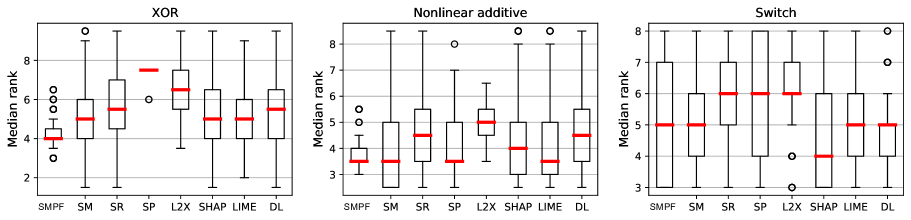
Figure 2: Box-plot of feature importance for three datasets. The red lines show the median ranks under each algorithm. Lower median ranks imply better performance. DL refers to DeepLIFT.

5.1 Metamodels for Fixed Functions

In this experiment, we find metamodels for four synthetic functions with two variables. We compare the performance of our method (SMPF) with symbolic metamodeling (SM), symbolic pursuit (SP), polynomial approximation of SP (SP^p), and symbolic regression (Orzechowski, La Cava, and Moore 2018) (similar to (Alaa and van der Schaar 2019) we use gplearn library (Stephens 2015) for implementation of SR). We compare methods in terms of mean squared error (MSE) and $R^{2}$ score. Generally, our algorithm achieves a better accuracy as compared to other methods (we have the best score for three of the functions). The results are reported in Table 1. Furthermore, SMPF was able to correctly identify the functional form. For the first experiment, the final expression of the metamodel is as follows (we rounded up coefficients here):

$$g(\bm{x})=0.854\exp\Big{(} -2.438\sin(1.371x_{0}-0.0318)+$$

$$\frac{0.684x_{1}}{0.016x_{1}^{2}+0.204x_{1}+0.426}\Big{)}.$$

This shows an important advantage of our method in comparison to other methods. For example, the expression found by SP algorithm has the following form ($P1$ here is a linear combination of the two inputs):

$$g(x)=0.98\,G^{2,1}_{2,3}\left({}^{\,\,\,\,0.24,-0.06}_{0.16,-0.47,0.43}\,|\,1.0[ReLU(P1)]\right).$$

Note that it was not possible to find a closed form expression for this function. Also, for the second function, $\sin$ is correctly chosen as the outer function in SMPF. See Appendix E, where we provide results for synthetic functions with more variables.

	Method	MLP		SVM
		MSE	$R^{2}$	MSE	$R^{2}$
Black Box		$0.689\pm 0.224$	$0.703\pm 0.019$	$0.448\pm 0.241$	$0.781\pm 0.061$
Method v.s. Black Box	$\begin{array}[]{c}\mbox{SMPF}\\ \mbox{SP}\end{array}$	$\begin{array}[]{c}0.007\pm 0.003\\ 0.008\pm 0.011\end{array}$	$\begin{array}[]{c}0.993\pm 0.003\\ 0.978\pm 0.016\end{array}$	$\begin{array}[]{c}0.029\pm 0.013\\ 0.014\pm 0.015\end{array}$	$\begin{array}[]{c}0.967\pm 0.120\\ 0.974\pm 0.078\end{array}$
Method	$\begin{array}[]{c}\mbox{SMPF}\\ \mbox{SP}\end{array}$	$\begin{array}[]{c}0.674\pm 0.211\\ 0.682\pm 0.225\end{array}$	$\begin{array}[]{c}0.709\pm 0.015\\ 0.697\pm 0.027\end{array}$	$\begin{array}[]{c}0.344\pm 0.163\\ 0.471\pm 0.253\end{array}$	$\begin{array}[]{c}0.829\pm 0.037\\ 0.780\pm 0.048\end{array}$

Table 2: Interpreting black-boxes trained on real data using SMPF compared with SP

5.2 Instance-wise Feature Selection

In this experiment, we evaluate the performance of our method for estimating the feature importance by repeating the second experiment of (Alaa and van der Schaar 2019). Three synthetic datasets are used: XOR, Nonlinear additive features, and Feature switching. All three datasets have 10 features, in XOR, only the first two features contribute in producing the output. In Nonlinear additive features and switch datasets, the first four features and first five features are important, respectively. First, we train a 2-layer neural network $f(\bm{x})$ with 200 hidden neurons for estimating the label of each data point. Then, we run our algorithm to find function $g(\bm{x})$ to estimate function $f(\bm{x})$. We consider the coefficient of each feature in the Taylor series of $g(\bm{x})$ as a metric for its importance. The larger the coefficient, the more important it will be. We rank the features based on their importance. We consider 1000 data points, repeat the process for each data point and find the median feature importance ranking. The median value of relevant features determines the accuracy of the algorithm; the smaller median rank implies a better accuracy. Figure 2 compares our algorithm with Symbolic Metamodeling (SM) (Alaa and van der Schaar 2019), Symbolic Pursuit (SP) (Crabbe et al. 2020), Symbolic Regression (Orzechowski, La Cava, and Moore 2018), DeepLIFT (Shrikumar, Greenside, and Kundaje 2017), SHAP (Lundberg and Lee 2017), LIME (Ribeiro, Singh, and Guestrin 2016b), and L2X (Chen et al. 2018). SMPF performs competitively comparing with other algorithms. For XOR dataset we have the best median rank, and we are among the best for nonlinear additive dataset. On Switch dataset, SMPF performs similar to other global methods, i.e., SM, SP, and SR which are our direct competitors. SHAP is the only algorithm that has a better performance on this dataset.

5.3 Black-box Approximation

In this experiment, we evaluate performance of our model on interpreting a black-box trained on real data, replicating the second experiment of (Crabbe et al. 2020). A Multilayer Perceptron (MLP), and Support Vector Machine (SVM) are trained as two black boxes using UCI dataset Yacht (Dua and Graff 2017) (additional results are reported in Appendix E). In order to have the same setting as SP, we train the MLP and SVM models using the scikit-learn library (Buitinck et al. 2013) with the default parameters. We randomly use 80% of the data points for the training of the black box model as well as SMPF model, and the remaining 20% is used to evaluate the performance of the model. This procedure is repeated five times to report the averages and standard deviations. We report the mean squared error (MSE) and $R^{2}$ score of the MLP and SVM against the true labels, MSE and $R^{2}$ of the metamodel against the black-box models, and the MSE and $R^{2}$ of the metamodel against the true labels (see Table 2). We observe that both SP and SMPF have very good performance in approximating the black-box. Interestingly, SMPF outperforms the black-box on the test set for both models which may indicate that the black-box overfits the dataset, but SMPF does not, as it uses simple functions.

6 Discussion

Complexity: In terms of run-time, for the last experiment, the training of SP for the MLP black-box takes 215 minutes, while the training of our algorithm takes 45 minutes (both performed on a personal computer). The reason that SP is more computationally expensive is that SP has to evaluate Meijer G-functions in each iteration of their optimization process. Evaluating a Meijer G-function is very expensive and takes about 1 to 4 seconds depending on the hyperparameters (i.e., $m,n,p,q$). This observation implies that SMPF has lower computational complexity which allows us to handle more variables and also enables the possibility of using more complex trees, as we suggest later in the future work. However, this should be highlighted that our method (similar to other symbolic methods) is not appropriate for high dimensional data like images.

Limitations: Even though we showed the performance of our model through extensive numerical experiments, our method lacks theoretical guarantees (theoretical analysis is particularly challenging because of the use of GP). Another limitation (also inherited from GP) is that there are several hyperparameters in our model to specify structure of the tree. As discussed, symbolic metamodels cannot handle high dimension inputs. Finally, the richness of functions we can create is limited, this can be compensated using more complex classes of functions or more complex tree structures.

Direct training vs using black-box: A natural question is why not directly use the training data to train the metamodel (without using the black-box)? There are two reasons for why we have considered the black-box for training. One is from the user point of view, we may have been given a task of interpreting a black-box, i.e., the user’s question may be why this particular method is working, and not necessarily looking for another interpretable method. Secondly, and more importantly, we may not have access to the dataset for various reasons including privacy concerns. In this method we only need querying the black-box method and we can use random inputs (as many of them as we want). Directly using the dataset in all symbolic metamodeling methods (e.g. SR, SM, and SP) is also possible and can be relevant in many scenarios, e.g., discovering the underlying governing rules of a dataset (Udrescu and Tegmark 2020a; Sahoo, Lampert, and Martius 2018; Makke, Sadeghi, and Chawla 2021).

Conclusion and future work: We proposed a new generic framework for symbolic metamodeling based on the Kolmogorov superposition theorem. We suggested using simple parameterized functions to get a closed-form and interpretable expression for the metamodel. The use of simple functions may seem restrictive when compared with SM and SP which use Meijer G-functions (a richer class of functions). However, this is compensated in our framework with a better approximation of KST. We used genetic programming to search over different possible trees and also possible classes of functions. There are several directions for the expansion of this work: 1) we can consider a more complex tree structure. For example, we can have trees with four layers instead of three, which allows us to construct more complex expressions (see Appendix D). 2) Other primitive functions can be used in our setup, e.g., Meijer G-functions. 3) The optimization in the training phase can be improved. The problem is non-convex, and gradient descent may not be able to find the global optimal point. This issue can be addressed by imposing convex relaxation or using more sophisticated non-convex optimization methods.

Acknowledgment: This work is partially supported by the NSF under grants IIS-2301599 and ECCS-2301601.

References

- Alaa and van der Schaar (2019) Alaa, A. M.; and van der Schaar, M. 2019. Demystifying Black-box Models with Symbolic Metamodels. In Advances in Neural Information Processing Systems, 11304–11314.
- Alvarez-Melis and Jaakkola (2018) Alvarez-Melis, D.; and Jaakkola, T. S. 2018. Towards robust interpretability with self-explaining neural networks. arXiv preprint arXiv:1806.07538.
- Alvarez-Melis and Jaakkola (2018) Alvarez-Melis, D.; and Jaakkola, T. S. 2018. Towards Robust Interpretability with Self-Explaining Neural Networks. In Proceedings of the 32nd Conference on Neural Information Processing Systems (NeurIPS), 7786–7795. Montréal, Canada.
- Arnaldo, Krawiec, and O’Reilly (2014) Arnaldo, I.; Krawiec, K.; and O’Reilly, U.-M. 2014. Multiple regression genetic programming. In Proceedings of the 2014 Annual Conference on Genetic and Evolutionary Computation, 879–886.
- Arrieta et al. (2020) Arrieta, A. B.; Díaz-Rodríguez, N.; Del Ser, J.; Bennetot, A.; Tabik, S.; Barbado, A.; García, S.; Gil-López, S.; Molina, D.; Benjamins, R.; et al. 2020. Explainable Artificial Intelligence (XAI): Concepts, taxonomies, opportunities and challenges toward responsible AI. Information Fusion, 58: 82–115.
- Beals and Szmigielski (2013) Beals, R.; and Szmigielski, J. 2013. Meijer G-functions: a gentle introduction. Notices of the AMS, 60(7): 866–872.
- Buitinck et al. (2013) Buitinck, L.; Louppe, G.; Blondel, M.; Pedregosa, F.; Mueller, A.; Grisel, O.; Niculae, V.; Prettenhofer, P.; Gramfort, A.; Grobler, J.; et al. 2013. API design for machine learning software: experiences from the scikit-learn project. arXiv preprint arXiv:1309.0238.
- Carmona et al. (2015) Carmona, V. I. S.; Rocktäschel, T.; Riedel, S.; and Singh, S. 2015. Towards Extracting Faithful and Descriptive Representations of Latent Variable Models. In AAAI Spring Symposium on Knowledge Representation and Reasoning: Integrating Symbolic and Neural Approaches. Palo Alto, California, USA.
- Chen et al. (2019) Chen, C.; Li, O.; Barnett, A.; Su, J.; and Rudin, C. 2019. This Looks Like That: Deep Learning for Interpretable Image Recognition. In Proceedings of the 33rd Conference on Neural Information Processing Systems (NeurIPS). Vancouver, Canada.
- Chen et al. (2018) Chen, J.; Song, L.; Wainwright, M.; and Jordan, M. 2018. Learning to explain: An information-theoretic perspective on model interpretation. In International Conference on Machine Learning, 883–892. PMLR.
- Chen, Xue, and Zhang (2015) Chen, Q.; Xue, B.; and Zhang, M. 2015. Generalisation and domain adaptation in GP with gradient descent for symbolic regression. In 2015 IEEE congress on evolutionary computation (CEC), 1137–1144. IEEE.
- Chen et al. (2011) Chen, X.; Ong, Y.-S.; Lim, M.-H.; and Tan, K. C. 2011. A multi-facet survey on memetic computation. IEEE Transactions on Evolutionary Computation, 15(5): 591–607.
- Crabbe et al. (2020) Crabbe, J.; Zhang, Y.; Zame, W.; and van der Schaar, M. 2020. Learning outside the Black-Box: The pursuit of interpretable models. Advances in Neural Information Processing Systems, 33.
- Craven and Shavlik (1996) Craven, M. W.; and Shavlik, J. W. 1996. Extracting tree-structured representations of trained networks. Advances in neural information processing systems, 24–30.
- Doshi-Velez and Kim (2017) Doshi-Velez, F.; and Kim, B. 2017. Towards a rigorous science of interpretable machine learning. arXiv preprint arXiv:1702.08608.
- Dua and Graff (2017) Dua, D.; and Graff, C. 2017. UCI Machine Learning Repository.
- Emigdio et al. (2014) Emigdio, Z.; Trujillo, L.; Schütze, O.; Legrand, P.; et al. 2014. Evaluating the effects of local search in genetic programming. In EVOLVE-A Bridge between Probability, Set Oriented Numerics, and Evolutionary Computation V, 213–228. Springer.
- Erhan et al. (2009) Erhan, D.; Bengio, Y.; Courville, A. C.; and Vincent, P. 2009. Visualising Higher-Layer Features of a Deep Network. Technical Report 1341, University of Montreal.
- Friedman and Stuetzle (1981) Friedman, J. H.; and Stuetzle, W. 1981. Projection pursuit regression. Journal of the American statistical Association, 76(376): 817–823.
- Guidotti et al. (2018) Guidotti, R.; Monreale, A.; Ruggieri, S.; Pedreschi, D.; Turini, F.; and Giannotti, F. 2018. Local rule-based explanations of black box decision systems. arXiv preprint arXiv:1805.10820.
- Kolmogorov (1957) Kolmogorov, A. N. 1957. On the representation of continuous functions of many variables by superposition of continuous functions of one variable and addition. In Doklady Akademii Nauk, volume 114, 953–956. Russian Academy of Sciences.
- Kommenda (2018) Kommenda, M. 2018. Local Optimization and Complexity Control for Symbolic Regression/eingereicht von Michael Kommenda. Ph.D. thesis, Universität Linz.
- Koza (1994) Koza, J. R. 1994. Genetic programming as a means for programming computers by natural selection. Statistics and computing, 4(2): 87–112.
- Lipton (2016) Lipton, Z. C. 2016. The Mythos of Model Interpretability. In Proceedings of the International Conference on Machine Learning (ICML) Workshop on Human Interpretability in Machine Learning. New York, USA.
- Lou et al. (2013) Lou, Y.; Caruana, R.; Gehrke, J.; and Hooker, G. 2013. Accurate intelligible models with pairwise interactions. In Proceedings of the 19th ACM SIGKDD international conference on Knowledge discovery and data mining, 623–631.
- Lundberg and Lee (2017) Lundberg, S.; and Lee, S.-I. 2017. A unified approach to interpreting model predictions. arXiv preprint arXiv:1705.07874.
- Makke, Sadeghi, and Chawla (2021) Makke, N.; Sadeghi, M. A.; and Chawla, S. 2021. Symbolic Regression for Interpretable Scientific Discovery. In International Conference on Big Data Analytics, 26–40. Springer.
- Meijer (1936) Meijer, C. 1936. Uber Whittakersche bezw. Besselsche funktionen und deren produkte (english translation: About whittaker and bessel functions and their products). Nieuw Archief voor Wiskunde, 18(2): 10–29.
- Meijer (1946) Meijer, C. 1946. On the G-function. North-Holland.
- Molnar (2019) Molnar, C. 2019. Interpretable Machine Learning: A Guide for Making Black Box Models Explainable. Accessed December 17, 2019.
- Montavon, Samek, and Müller (2018) Montavon, G.; Samek, W.; and Müller, K.-R. 2018. Methods for Interpreting and Understanding Deep Neural Networks. Digital Signal Processing, 73: 1–15.
- Mundhenk et al. (2021) Mundhenk, T. N.; Landajuela, M.; Glatt, R.; Santiago, C. P.; Faissol, D. M.; and Petersen, B. K. 2021. Symbolic regression via neural-guided genetic programming population seeding. arXiv preprint arXiv:2111.00053.
- Orzechowski, La Cava, and Moore (2018) Orzechowski, P.; La Cava, W.; and Moore, J. H. 2018. Where are we now? A large benchmark study of recent symbolic regression methods. In Proceedings of the Genetic and Evolutionary Computation Conference, 1183–1190.
- Petersen et al. (2021) Petersen, B. K.; Larma, M. L.; Mundhenk, T. N.; Santiago, C. P.; Kim, S. K.; and Kim, J. T. 2021. Deep symbolic regression: Recovering mathematical expressions from data via risk-seeking policy gradients. In International Conference on Learning Representations.
- Rad, Feng, and Iba (2018) Rad, H. I.; Feng, J.; and Iba, H. 2018. GP-RVM: Genetic programing-based symbolic regression using relevance vector machine. arXiv preprint arXiv:1806.02502.
- Ribeiro, Singh, and Guestrin (2016a) Ribeiro, M. T.; Singh, S.; and Guestrin, C. 2016a. Model Agnostic Interpretability of Machine Learning. In Proceedings of the International Conference on Machine Learning (ICML) Workshop on Human Interpretability in Machine Learning. New York, USA.
- Ribeiro, Singh, and Guestrin (2016b) Ribeiro, M. T.; Singh, S.; and Guestrin, C. 2016b. Why should i trust you?” Explaining the predictions of any classifier. In Proceedings of the 22nd ACM SIGKDD international conference on knowledge discovery and data mining, 1135–1144.
- Rudin (2019) Rudin, C. 2019. Stop Explaining Black Box Machine Learning Models for High Stakes Decisions and Use Interpretable Models Instead. Nature Machine Intelligence, 1(5): 206–215.
- Sahoo, Lampert, and Martius (2018) Sahoo, S.; Lampert, C.; and Martius, G. 2018. Learning equations for extrapolation and control. In International Conference on Machine Learning, 4442–4450. PMLR.
- Schmidt and Lipson (2009) Schmidt, M.; and Lipson, H. 2009. Distilling free-form natural laws from experimental data. science, 324(5923): 81–85.
- Shrikumar, Greenside, and Kundaje (2017) Shrikumar, A.; Greenside, P.; and Kundaje, A. 2017. Learning important features through propagating activation differences. In International Conference on Machine Learning, 3145–3153. PMLR.
- Stephens (2015) Stephens, T. 2015. Gplearn Model, genetic programming.
- Thrun (1995) Thrun, S. 1995. Extracting rules from artificial neural networks with distributed representations. Advances in neural information processing systems, 505–512.
- Topchy and Punch (2001) Topchy, A.; and Punch, W. F. 2001. Faster genetic programming based on local gradient search of numeric leaf values. In Proceedings of the genetic and evolutionary computation conference (GECCO-2001), volume 155162. Morgan Kaufmann.
- Udrescu and Tegmark (2020a) Udrescu, S.-M.; and Tegmark, M. 2020a. AI Feynman: A physics-inspired method for symbolic regression. Science Advances, 6(16): eaay2631.
- Udrescu and Tegmark (2020b) Udrescu, S.-M.; and Tegmark, M. 2020b. Symbolic Pregression: Discovering Physical Laws from Distorted Video. arXiv e-prints, arXiv–2005.
- Wang, Wagner, and Rondinelli (2019) Wang, Y.; Wagner, N.; and Rondinelli, J. M. 2019. Symbolic regression in materials science. MRS Communications, 9(3): 793–805.
- Zhang, Solar-Lezama, and Singh (2018) Zhang, X.; Solar-Lezama, A.; and Singh, R. 2018. Interpreting neural network judgments via minimal, stable, and symbolic corrections. arXiv preprint arXiv:1802.07384.